Photometric study of fourteen low-mass binaries

Abstract

New CCD photometric observations of fourteen short-period low-mass eclipsing binaries (LMB) in the photometric filters I, R and V were used for the light curve analysis. There still exists a discrepancy between radii as observed and those derived from the theoretical modelling for LMB in general. Mass calibration of all observed LMB was done using only the photometric indices. The light curve modelling of these selected systems were performed, yielding the new derived masses and radii for both components. We compared these systems with the compilation of other known double-lined LMB systems with uncertainties of masses and radii less then 5 %, which includes 66 components of binaries where both spectroscopy and photometry were combined together. All of our systems are circular short-period binaries, and for some of them the photospheric spots were also used. A purely photometric study of the light curves without spectroscopy seems unable to achieve high enough precision and accuracy in the masses and radii to provide for a meaningful test of the M-R relation for low-mass stars.

1. Introduction

Low-mass stars ($M\lesssim 1.0\,M_{\astrosun}$, Morales et al., 2011) are the most common type of stars (Kroupa et al., 2013). Despite this fact, it seems that models describing the evolution of the stars are not sufficiently robust and show inconsistencies around 3 % in radius at a fixed mass and up to 10 % in some cases (Feiden & Chaboyer, 2012; Spada et al., 2013). This can be explained by the presence of large-scale magnetic fields that reduce convective efficiency and induce stellar spots on the surfaces of the stars (see e.g. Chabrier et al. (2007) or Torres et al. (2010). These phenomena are not often included in models of stellar evolution as well as the rotation of stars. Inconsistency appears to be more apparent for close binary systems due to the high rotation velocity. Rotation period is synchronized with the orbital period due to the tidal forces.

To date, over sixty of such components were observed both via spectroscopy and photometry together and analysed simultaneously, yielding the precise and accurate (uncertainties of masses and radii less than 5 %) values of masses and radii. The main motivation of this work was the easy availability of a large number of high-precision photometric observations (for example from the Kepler survey), in which a large number of LMB was detected (Coughlin et al., 2011). Therefore, we decided to test whether the M-R relation discrepancy could be observed also from the sole ground-based photometry.

2. Data

All new photometric observations of fourteen binaries were carried out in the Ondřejov Observatory in the Czech Republic with the 0.65-m reflecting-type telescope and the G2-3200 CCD camera. Observations were collected from Feb 2015 to Nov 2016 in filters I, R and V (Bessell, 1990). Some of the older observations obtained only in R filter were used for refining the individual orbital periods.

The stars were chosen mainly from the catalog of Hoffman et al. (2008). For the selection of suitable stars we used several criteria. Its classification as a low-mass binary was done using the photometric indices $J-H$ and $H-K$ which are known from the 2MASS survey (Cutri et al., 2003) ($J-H>0.25$ and $H-K>0.07$ Pecaut & Mamajek (2013)). Furthermore, we selected binary systems which have short orbital periods ($P<1.5$ days). There were two reasons for this: First, we wanted to analyse as many systems as possible, and secondly, discrepancy should be more apparent for the short-period systems. We did not consider observing binaries with longer orbital periods. Furthermore, we chose the declination to be higher than $+$30^∘. This guaranteed that the systems are easily observable throughout most of the year from our observatory. The last criterion was that these systems were not analysed in detail before. We chose eleven systems in Hoffman’s catalog, two more were found in measured field (one of them is on the edge of criteria) and one star was added later.

An example of the individual data are listed in Table 1. Some more details about the observations are listed in Table LABEL:tab:summary.

Table 1A sample of photometric observations for NSVS 363024, filter I.

$H\!J\!D$	$\Delta\mathrm{m}$	$\sigma\left(\Delta\mathrm{m}\right)$
$[-2400000]$	$[\mathrm{mag}]$	$[\mathrm{mag}]$
57262.2917	0.6499	0.0076
57262.2930	0.6657	0.0070
57262.2946	0.6580	0.0065
57262.2955	0.6541	0.0052
57262.2968	0.6605	0.0090
57262.2981	0.634	0.013
57262.2994	0.6296	0.0075
57262.3033	0.6451	0.0044
57262.3052	0.6577	0.0043
57262.3065	0.6582	0.0044
All photometric observations are available on-line.

3. Analysis

Standard calibration (dark frame, flat field) was applied to the observed frames. The light curves were obtained using an aperture photometry (Motl, 2011). As a comparison star we chose a star which satisfies (as best as possible) the following conditions. That star should be as bright as the binary. And spectral type of comparison and binary must be the same. Of course, comparison’s brightness is constant.

The light curves were analysed using the program PHOEBE (Prša & Zwitter, 2005), which is based on the Wilson-Devinney algorithm (Wilson & Devinney, 1971). The temperature of the primary component was (similarly to mass) calibrated from the above mentioned tables. Orbital periods were known with only a small accuracy from the Hoffman’s publication. Better precision was achieved using the methods of minimizing the phase dispersion and construction of the $O-C$ diagrams (used minima are in Table LABEL:tab:minima). PHOEBE is not designed for determining the orbital period.

No spectroscopic observations were obtained for our selected systems. To estimate the individual component masses we assumed relation between the infrared photometric indices $J-H$ and $H-K$ and mass. For calibration of masses we used large tables of these indices on the website mentioned above. Here are the rules for deriving the mass and its uncertainty:

• Write masses which correspond to the photometric indices (including an error) using the tables. These two intervals (one for each index) are $I_{1}$ and $I_{2}$.

• 1. $I_{3}=I_{1}\cap I_{2}=I_{1}$ or $I_{3}=I_{1}\cap I_{2}=I_{2}$: then mass is average of $M_{1}$ and $M_{2}$.

  $$M_{1}=\left[\min(I_{3})+\max(I_{3})\right]/2$$ (1)

• 2. $I_{1}\cap I_{2}\neq I_{1}$ or $I_{1}\cap I_{2}\neq I_{2}$: then $\min(I_{i})<\min(I_{j})<\max(I_{i})<\max(I_{j})$. Then mass can be estimate as a weighted average where weights are lengths of the intervals:

  $$\begin{split}M_{1}&=\frac{\max(I_{i})/\left[\max(I_{i})-\min(I_{i})\right]}{1/\left[\max(I_{i})-\min(I_{i})\right]+1/\left[\max(I_{j})-\min(I_{j})\right]}\\ &+\frac{\min(I_{j})/\left[\max(I_{j})-\min(I_{j})\right]}{1/\left[\max(I_{i})-\min(I_{i})\right]+1/\left[\max(I_{j})-\min(I_{j})\right]}\end{split}$$ (2)

• 3. $I_{1}\cap I_{2}=\emptyset$: then $\min(I_{i})<\max(I_{i})<\min(I_{j})<\max(I_{j})$. Again, mass will be estimated as a weighted average:

  $$\begin{split}M_{1}&=\frac{\max(I_{i})/\left[\max(I_{i})-\min(I_{i})\right]}{1/\left[\max(I_{i})-\min(I_{i})\right]+1/\left[\max(I_{j})-\min(I_{j})\right]}\\ &+\frac{\min(I_{j})/\left[\max(I_{j})-\min(I_{j})\right]}{1/\left[\max(I_{i})-\min(I_{i})\right]+1/\left[\max(I_{j})-\min(I_{j})\right]}\end{split}$$ (3)

• Lower/Upper uncertainty was estimated similarly. For lower limit:

  $$\begin{split}\sigma(M_{1})&=\frac{\left|M_{1}-\min(I_{1})\right|/\left[\max(I_{1})-\min(I_{1})\right]}{1/\left[\max(I_{1})-\min(I_{2})\right]+1/\left[\max(I_{2})-\min(I_{2})\right]}\\ &+\frac{\left|M_{1}-\min(I_{2})\right|/\left[\max(I_{2})-\min(I_{2})\right]}{1/\left[\max(I_{1})-\min(I_{2})\right]+1/\left[\max(I_{2})-\min(I_{2})\right]}\end{split}$$ (4)

  For upper limit there are $\max$ in absolute values instead of $\min$. Same rule was used for $\sigma(T)$ and $\sigma\left(M_{\mathrm{bol}}\right)$. In these cases we calculated average of lower and upper uncertainties.

• Mass of secondary component is computed as $M_{2}~{}=~{}M_{1}~{}\cdot~{}q$ and we used propagation of uncertainties (we assumed $\sigma(q)=0.05$).

We deal with the effect, that seems to be caused by magnetic fields. Therefore, we must take into account the presence of stellar spots that deform the light curve. For the asymmetric light curves the stellar spots were considered as a hypothesis. However, the suitability of placing the spot(s) was tested using the so-called BIC criterion (Schwarz, 1978) which connects the resulting chi-square with the number of parameters used and the degrees of freedom.

Firstly, we assume that the mass ratio is equal to 1. We then let the model parameters converge so that the theoretical curve coincides with the observed one. Because the mass ratio is probably not equal to 1, we used the M-L relation in the form

$$\log q=\frac{\log L_{\mathrm{bol}_{2}}-\log L_{\mathrm{bol}_{1}}}{4.841}$$ (5)

where $L_{\mathrm{bol}_{1}}$ and $L_{\mathrm{bol}_{2}}$ are the bolometric luminosities. The equation was modified according to Graczyk (2003) and Eker et al. (2015). Then again we let the model parameters converge and the process is repeated until the mass ratio changes were negligible (less than 0.02) and the best $\chi^{2}$ value was obtained.

We describe the analysis of one system (NSVS 363024) step by step. Then some interesting systems were chosen and briefly mentioned in the following sections 4.1-4.7.

NSVS 363024 was observed between 31st Jan 2015 and 25th July 2016 (see Table 8). In this period we measured three primary and two secondary minima (Table LABEL:tab:minima). All images were processed in a standard way. We applied correction frames, chose a suitable comparison star and aperture. Then we obtained the light curves for each photometric filter. All the observed minima were used for refining the orbital period via an $O-C$ diagram analysis. Depending on the remoteness in time of observed minima, we have refined the orbital period of one to two orders of magnitude (compare values in Table 2 and Table 3).

After that we estimate the mass and temperature of primary using the photometric indices (only $J-H$ and $H-K$ was known), as described above. We let the mass ratio equal to one and set reflection effect with 2 reflections. Fine and course grid raster for both components were set to 30. We started with hypothesis that NSVS 363024 is a detached binary system and chose this model as one of option of PHOEBE. We checked this hypothesis during the whole fitting process. All the available photometric filters were fitted simultaneously. At first, we fitted parameters that have a significant effect on the light curve. These are the relative luminosity of components $L_{1}$ and $L_{2}$, inclination $i$, surface gravity potentials $\Omega_{1}$ and $\Omega_{2}$ and temperature of secondary component $T_{2}$. Further, we let converge parameters of the second order (albedos $A_{i}$, coefficients of gravitational darkening $g_{i}$ and parameters of synchronicity $F_{i}$). They have considerable errors often, because our photometric observations were affected by observing conditions. Then we fitted some of first order parameters again and some of second order parameters but the values in the correlation matrix of these parameters should not exceed 0.7 and cannot exceed 0.8. This criterion selected groups of parameters which could be and were fitted together. Next, we can try to fit the third light $L_{3}$ and add a stellar spot. Spot’s parameters could be estimated from asymmetry of the light curve. Because the effective temperature and radius of a spot are correlated we assumed that ratio of spot temperature and star temperature is higher than $0.65$ analogically to the sunspots. The ratio should by even higher for cooler stars (Berdyugina, 2005). Finally, when the fit of the light curve is as good as it can be we change value of mass ratio as it is determined by Eq. 5. The whole procedure was repeated until the changes of the mass ratio are negligible. Then we can add more stellar spots and repeat the procedure. But we had to check the BIC criterion for optimal number of spots. Limb darkening coefficient was derived via tables published by van Hamme (1993). The whole fitting process was finished when $\chi^{2}$ stopped decreasing its value and residuals are symmetric around the zero value. A very similar process was applied to all systems.

We also try to fix the second order parameters ($F_{i}=1$, $A_{i}=0.6$ and $g_{i}=0.32$) and carry out the analysis again. We did not change number of spots. The results are given in Table 6. Changes of values of masses and radii are smaller than their uncertainties in many cases. It is the same for bolometric magnitudes and temperatures. There are two systems (NSVS 2517147 and NSVS 3630887) with significant change of radius (secondary components only). Their radius increase of about 0.1 $R_{\astrosun}$ and mass of the components increase of 0.04 $M_{\astrosun}$ and 0.07 $M_{\astrosun}$. The alternative solutions still give radii for these two binaries in disagreement with the models.

4. Individual systems

Table 2 summarizes basic information about the studied systems and Table 8 contains basic information about our observations. Some interesting systems were briefly described in the following subsections.

Table 2Basic properties of systems from Hoffman et al. (2008) and Cutri et al. (2003) catalogs.

System	RA	DE	$J-H$	$H-K$	$V$	$P$
	[h m s]	[$\circ$ $\prime$ $\prime\prime$]	[mag]	[mag]	[mag]	[days]
2MASS J01535799 +7146169	01 53 57.99	$+$71 46 17.02	0.523 (59)	0.099 (81)	-	-
NSVS 363024	01 53 58.91	$+$71 41 26.01	0.590 (36)	0.114 (35)	12.744 (41)	0.433190
NSVS 401928	03 26 18.02	$+$69 56 21.24	0.460 (37)	0.163 (38)	13.014 (52)	0.578880
V0345 Cam	04 25 55.35	$+$69 15 45.51	0.545 (40)	0.209 (40)	13.361 (72)	0.451570
NSVS 2285307	06 09 21.56	$+$58 32 54.81	0.483 (81)	0.256 (79)	13.441 (81)	0.646210
NSVS 2517147	09 19 31.31	$+$57 17 30.24	0.477 (28)	0.139 (26)	13.048 (47)	0.446730
GK CVn	14 00 48.19	$+$33 47 22.10	0.559 (29)	0.104 (31)	$\sim$14.45000  (0)	0.401288
V0514 Dra	17 19 54.84	$+$69 47 42.65	0.453 (25)	0.075 (25)	12.941 (69)	0.314220
NSVS 3151384	20 19 49.09	$+$65 34 14.28	0.620 (50)	0.120 (40)	11.305 (16)	1.250790
2MASS J20333510 +4839427	20 33 35.10	$+$48 39 42.73	0.248 (38)	0.098 (38)	-	-
NSVS 5789962	20 33 36.26	$+$48 45 33.10	0.282 (37)	0.044 (36)	12.160 (38)	1.456680
NSVS 3243815	20 38 57.73	$+$58 04 56.74	0.510 (26)	0.124 (29)	13.177 (76)	0.863940
NSVS 6127971	22 49 56.89	$+$38 43 48.36	0.468 (78)	0.153 (76)	12.692 (41)	0.541860
NSVS 3630887	23 55 39.53	$+$39 12 10.62	0.611 (34)	0.173 (32)	12.439 (32)	0.460300

4.1. NSVS 363024

NSVS 363024 (2MASS J01535891+7141260) is an eclipsing binary in Cassiopeia constellation. Its maximum brightness in filter V is 12.744 mag. There is not a single detailed publication about this binary, so the spectral type is unknown. It was estimated from the photometric indices. From the above described analysis it revealed that NSVS 363024 is a detached binary system. Light curve shows asymmetry, which was explained via a presence of a stellar spot. Half a year after the last measurement of the secondary minimum we measured that part of the curve twice again. Both observations were carried out in good weather conditions. The shape of the newly measured minima does not coincide with the shape of the minimum which was measured earlier (see Fig. 1 for comparison). Such a spot variability on the timescale of hundreds of days was observed on several other systems, see e.g. Künstler et al. (2015).

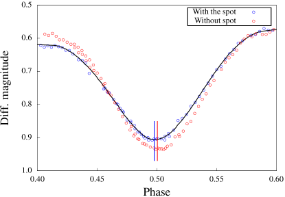
Figure 1.— Secondary minimum of NSVS 363024. There is outlined a difference in mid-eclipse times in both cases. The difference is about 95 seconds. Times of minima were computed as minimum of a polynomial fitting of the direct and mirror image light curves.

4.2. V0345 Cam

V0345 Cam (2MASS J04255534+6915455) is a detached system with its brightness of 13.361 mag in filter V. Two primary and three secondary minima were observed from 17 Apr 2015 to 19 Jan 2016. Both photometric indices gave us nearly the same masses and effective temperatures. Due to this fact only small uncertainties of masses and temperatures were calculated.

4.3. NSVS 2285307

NSVS 2285307 (2MASS J06092156+5832548) is a detached binary with the orbital period around 0.646 days. Its brightness in filter V is 13.441 mag. Data were carried out from 25 Feb 2015 to 09 Dec 2015 and we obtained three primary minima and two secondary minima. It allowed us to refined the orbital period about two orders of magnitude. The light curves of this system were asymmetric. This was explained by a spot on the surface of primary component. Its properties (and properties of others’ spots) are in Table 4. Significant value of the third light (around 16 %) was also detected. We did not find a star which is in the vicinity of the target which can be identified with the high level of the third light. It would be fruitful to carry out spectroscopy and test this hypothesis.

4.4. V0514 Dra

V0514 Dra (2MASS J17195483+6947426) is a W UMa type binary whose brightness in filter $\mathrm{V}_{\mathrm{max}}$ is 12.941 mag. We observed two primary and two secondary minima. On the light curve there is a slight asymmetry which was described by a hot spot on the surface of the primary component. This is the only hot spot as emerged from our analysis.

4.5. NSVS 3151384

NSVS 3151384 (2MASS J20194908+6534142) is a typical detached system. Its brightness in filter V is 11.305 mag. Likewise as in the previous case we monitored two primary and two secondary minima. We found very high value of a third light. It is due to a star which is very close to NSVS 3151384. Angular distance of these stars is less than 0.1 $\mathrm{arcmin}$.

4.6. NSVS 3243815

NSVS 324815 (2MASS J20385772+5804567) is another detached binary in our sample. Its light curves were slightly asymmetric (see Fig. 3) but we were not able to fit the curves with only one spot. We covered four primary minima and one secondary minimum. There was not any evolution of these spots in nearly two hundred days of the observational span.

4.7. NSVS 3630887

NSVS 3630887 (2MASS J23553953+3912106) is a detached binary. Maximum brightness of this system is 12.439 mag in filter V. We observed one primary and one secondary minimum and two incomplete secondary minima. The light curve of this system is strongly asymmetric. It was explained via only one spot on the surface of primary component. There was also detected a low value of the third light (only 2 % of the luminosity). This small value could be caused by imprecise data.

5. Results and discussion

The parameters of binaries we studied are summarized in the Tables 3 and 5, their light curves are shown in Fig. 3. Properties of spots are listed in the Table 4. There are only values of luminosities in the filter R because the scatter of the data was the smallest and values of luminosity in other filters are nearly the same as in the filter R (the differences are few percent only). Mass ratio $q$ was calculated from Eq. (5) and its values are from 0.84 to 1.00.

Table 3Parameters of binaries (PHOEBE results).

System	$H\!J\!D_{0}$	$P$	$i$	$\Omega_{1}$	$\Omega_{2}$	L1	L2	L3	Spot
	[$-2400000$]	[days]	[deg]			[%]	[%]	[%]	Y/N
2MASS J01535799 +7146169	57268.5300 (52)	0.2766000	67.38 (71)	3.710 (11)	3.710 (11)	$\sim$50	$\sim$50	000	N
NSVS 363024	57268.4824 (42)	0.4332050	77.06 (45)	4.298 (57)	4.643 (62)	$\sim$63	$\sim$37	000	Y
NSVS 401928	57117.4185 (31)	0.5788356	71.09 (43)	3.552 (37)	3.636 (42)	$\sim$67	$\sim$33	000	N
V0345 Cam	57297.4721 (37)	0.4515810	75.63 (51)	4.781 (42)	4.657 (36)	$\sim$55	$\sim$45	000	N
NSVS 2285307	57135.3155 (42)	0.6462444	87.05 (92)	4.761 (36)	5.693 (39)	$\sim$51	$\sim$33	$\sim$16	Y
NSVS 2517147	57070.5801 (35)	0.4466960	78.56 (42)	3.758 (29)	3.841 (26)	$\sim$76	$\sim$24	000	Y
GK CVn	57499.5681 (35)	0.4012861	76.70 (26)	4.856 (62)	3.751 (73)	$\sim$75	$\sim$25	000	N
V0514 Dra	57089.4184 (49)	0.3142184	85.22 (76)	3.536 (47)	3.536 (47)	$\sim$50	$\sim$50	000	Y
NSVS 3151384	57206.4214 (41)	1.2504940	84.17 (93)	7.047 (84)	6.466 (75)	$\sim$30	$\sim$32	$\sim$38	N
2MASS J20333510 +4839427	57503.1674 (39)	0.5417250	62.91 (51)	3.552 (41)	3.552 (41)	$\sim$68	$\sim$32	000	N
NSVS 5789962	57294.4378 (51)	1.4563260	89.34 (86)	4.974 (64)	5.396 (72)	$\sim$68	$\sim$32	000	N
NSVS 3243815	57238.8913 (37)	0.8640840	87.01 (62)	6.402 (41)	6.386 (72)	$\sim$52	$\sim$48	000	Y
NSVS 6127971	57296.4832 (21)	0.5417320	80.01 (55)	4.203 (41)	4.537 (43)	$\sim$60	$\sim$40	000	N
NSVS 3630887	57275.5392 (30)	0.4601950	78.62 (31)	3.806 (37)	5.070 (38)	$\sim$67	$\sim$31	0$\sim$2	Y

Table 4Spots properties.

System	Component	Colatitude	Longitude	Radius	Temperature
	prim/sec	[deg]	[deg]	[deg]	$T_{\mathrm{spot}}/T_{\mathrm{photosphere}}$
NSVS 363024	prim	70	225	17	0.820
NSVS 2285307	prim	38	277	20	0.724
NSVS 2517147	prim	141	118	28	0.711
V0514 Dra	prim	139	209	18	1.113
NSVS 3243815	prim	120	130	18	0.732
	sec	81	121	25	0.927
NSVS 3630887	sec	92	134	33	0.650

Table 5Absolute parameters of binaries.

System	$M_{1}$	$M_{2}$	$R_{1}$	$R_{2}$	$M_{\mathrm{bol}_{1}}$	$M_{\mathrm{bol}_{2}}$	$T_{1}$	$T_{2}$
	[$M_{\astrosun}$]	[$M_{\astrosun}$]	[$R_{\astrosun}$]	[$R_{\astrosun}$]	[mag]	[mag]	[K]	[K]
2MASS J01535799 +7146169	0.76 $\left({}^{+12}_{-05}\right)$	0.76 $\left({}^{+13}_{-06}\right)$	0.80 (08)	0.79 (08)	6.08. (78)	6.09. (78)	4750 (fixed)	4750 (fixed)
NSVS 363024	0.72 $\left({}^{+07}_{-07}\right)$	0.66 $\left({}^{+07}_{-07}\right)$	0.80 (04)	0.69 (03)	6.32. (72)	6.81. (60)	4500 (fixed)	4309.. (387)
NSVS 401928	0.77 $\left({}^{+06}_{-06}\right)$	0.67 $\left({}^{+07}_{-07}\right)$	1.27 (09)	1.13 (08)	5.10 (1.1)	5.720 (53)	4750 (fixed)	4334.. (288)
V0345 Cam	0.44 $\left({}^{+03}_{-01}\right)$	0.42 $\left({}^{+03}_{-02}\right)$	0.62 (03)	0.63 (03)	7.95. (97)	8.10. (83)	3500 (fixed)	3371.. (36)
NSVS 2285307	0.70 $\left({}^{+14}_{-14}\right)$	0.64 $\left({}^{+13}_{-13}\right)$	0.93 (06)	0.77 (05)	6.3. (1.0)	6.8. (1.1)	4200 (fixed)	4140.. (668)
NSVS 2517147	0.80 $\left({}^{+02}_{-02}\right)$	0.67 $\left({}^{+04}_{-04}\right)$	1.02 (03)	0.93 (03)	5.46. (57)	6.440 (48)	4850 (fixed)	4064.. (111)
GK CVn	0.73 $\left({}^{+15}_{-15}\right)$	0.67 $\left({}^{+14}_{-14}\right)$	0.66 (05)	0.89 (06)	6.7. (1.1)	7.1. (1.4)	4550 (fixed)	3547.. (472)
V0514 Dra	0.76 $\left({}^{+07}_{-07}\right)$	0.76 $\left({}^{+08}_{-08}\right)$	0.89 (05)	0.91 (05)	5.85. (49)	5.85. (49)	4750 (fixed)	4750 (fixed)
NSVS 3151384	0.70 $\left({}^{+08}_{-08}\right)$	0.70 $\left({}^{+09}_{-09}\right)$	0.90 (07)	1.00 (08)	6.34. (95)	6.2. (1.0)	4200 (fixed)	4090.. (401)
2MASS J20333510 +4839427	1.12 $\left({}^{+10}_{-18}\right)$	0.96 $\left({}^{+10}_{-17}\right)$	1.40 (09)	1.31 (08)	3.84. (66)	4.64. (66)	6000 (fixed)	5167.. (321)
NSVS 5789962	1.04 $\left({}^{+18}_{-07}\right)$	0.89 $\left({}^{+16}_{-08}\right)$	1.66 (08)	1.33 (07)	3.7. (1.2)	4.48. (61)	5750 (fixed)	5315.. (322)
NSVS 3243815	0.76 $\left({}^{+04}_{-03}\right)$	0.75 $\left({}^{+06}_{-05}\right)$	0.81 (03)	0.80 (04)	6.04. (36)	6.13. (29)	4750 (fixed)	4690.. (177)
NSVS 6127971	0.80 $\left({}^{+09}_{-12}\right)$	0.74 $\left({}^{+10}_{-12}\right)$	1.00 (05)	0.89 (05)	5.50. (77)	5.90. (73)	4850 (fixed)	4692.. (475)
NSVS 3630887	0.64 $\left({}^{+06}_{-06}\right)$	0.54 $\left({}^{+06}_{-06}\right)$	0.90 (04)	0.56 (03)	6.51. (99)	7.44. (50)	4050 (fixed)	4157.. (237)

Table 6Absolute parameters of binaries with fixed values of second order parameters.

System	$M_{1}$	$M_{2}$	$R_{1}$	$R_{2}$	$M_{\mathrm{bol}_{1}}$	$M_{\mathrm{bol}_{2}}$	$T_{1}$	$T_{2}$
	[$M_{\astrosun}$]	[$M_{\astrosun}$]	[$R_{\astrosun}$]	[$R_{\astrosun}$]	[mag]	[mag]	[K]	[K]
2MASS J01535799 +7146169	0.76 $\left({}^{+12}_{-05}\right)$	0.76 $\left({}^{+13}_{-06}\right)$	0.80 (08)	0.80 (09)	6.08. (78)	6.08. (78)	4750 (fixed)	4750 (fixed)
NSVS 363024	0.72 $\left({}^{+07}_{-07}\right)$	0.67 $\left({}^{+07}_{-07}\right)$	0.78 (04)	0.73 (03)	6.35. (70)	6.73. (60)	4500 (fixed)	4277.. (384)
NSVS 401928	0.77 $\left({}^{+06}_{-06}\right)$	0.69 $\left({}^{+07}_{-07}\right)$	1.24 (09)	1.18 (09)	5.10 (1.1)	5.610 (62)	4750 (fixed)	4350.. (289)
V0345 Cam	0.44 $\left({}^{+03}_{-01}\right)$	0.42 $\left({}^{+03}_{-02}\right)$	0.60 (03)	0.59 (03)	8.01. (92)	8.26. (68)	3500 (fixed)	3345.. (36)
NSVS 2285307	0.70 $\left({}^{+14}_{-14}\right)$	0.61 $\left({}^{+13}_{-13}\right)$	0.99 (07)	0.78 (05)	6.2. (1.1)	6.8. (1.1)	4200 (fixed)	4052.. (654)
NSVS 2517147	0.80 $\left({}^{+02}_{-02}\right)$	0.71 $\left({}^{+04}_{-04}\right)$	0.98 (03)	1.04 (03)	5.56. (47)	6.180 (24)	4850 (fixed)	4065.. (111)
GK CVn	0.73 $\left({}^{+15}_{-15}\right)$	0.70 $\left({}^{+15}_{-15}\right)$	0.63 (05)	0.95 (07)	6.8. (1.2)	6.9. (1.3)	4550 (fixed)	3564.. (474)
V0514 Dra	0.76 $\left({}^{+07}_{-07}\right)$	0.76 $\left({}^{+08}_{-08}\right)$	0.89 (05)	0.89 (05)	5.84. (50)	5.84. (50)	4750 (fixed)	4750 (fixed)
NSVS 3151384	0.70 $\left({}^{+08}_{-08}\right)$	0.70 $\left({}^{+09}_{-09}\right)$	0.91 (07)	1.01 (08)	6.33. (95)	6.2. (1.0)	4200 (fixed)	4094.. (401)
2MASS J20333510 +4839427	1.12 $\left({}^{+10}_{-18}\right)$	0.99 $\left({}^{+10}_{-17}\right)$	1.40 (09)	1.33 (08)	3.85. (66)	4.44. (66)	6000 (fixed)	5373.. (333)
NSVS 5789962	1.04 $\left({}^{+18}_{-07}\right)$	0.89 $\left({}^{+16}_{-08}\right)$	1.68 (08)	1.35 (08)	3.6. (1.2)	4.44. (61)	5750 (fixed)	5342.. (324)
NSVS 3243815	0.76 $\left({}^{+04}_{-03}\right)$	0.76 $\left({}^{+06}_{-05}\right)$	0.77 (03)	0.85 (04)	6.17. (26)	6.00. (39)	4750 (fixed)	4689.. (177)
NSVS 6127971	0.80 $\left({}^{+09}_{-12}\right)$	0.74 $\left({}^{+09}_{-12}\right)$	1.02 (05)	0.87 (05)	5.46. (80)	5.90. (73)	4850 (fixed)	4754.. (482)
NSVS 3630887	0.64 $\left({}^{+06}_{-06}\right)$	0.60 $\left({}^{+07}_{-06}\right)$	0.85 (04)	0.67 (03)	6.64. (86)	6.95. (57)	4050 (fixed)	4253.. (245)

5.1. M-R relation

In Fig. 2 (top left) there are masses and radii of measured stars. Grey lines connect the components of one binary. The curves in the figure are theoretically calculated M-R relation for single stars evolution for five billion years after ZAMS for three different values of metallicity (Spada et al., 2013). The values of radii are independent on metallicity for masses lower than approximately $0.7\,M_{\astrosun}$. Hence, we did not take any assumptions of metallicities. Although the theoretical curves are calculated for the given age, it is a good approximation for LMB due to their slow evolution. But the difference caused by evolution can be significant for solar-type stars (four of the studied components).

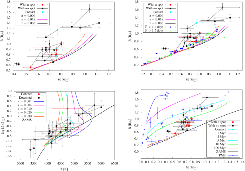
Figure 2.— Top left: Masses and radii of measured stars. Components of a binary are connected by grey lines. The theoretical curves were calculated for five billion years old single stars with different values of metallicities.
Top right: Comparison of our results with another systems for which photometry and spectroscopy were analysed simultaneously.
Bottom left: H-R diagram. Models were computed via Evolve ZAMS code (Paxton, 2004) for $M=0.6\,M_{\astrosun}$.
Bottom right: M-R relation for PMS stars. Models were adopted from Stassun et al. (2014).

Only one of the measured star is not located above the theoretical curves of the M-R relation. The discrepancy is not more evident for components with the spots on the surface. For five systems there is a component with and a component without the spot. For three of these systems spot-covered component is further from the curve but in two cases it is the opposite case. Uncertainties of masses of primary components are from 3 % to 20 % and secondary components from 7 % to 21 %. In only few cases the accuracy is good enough to study M-R discrepancy. Hence, it seems that sole photometry cannot be a suitable method for studying the M-R relation discrepancy. In Fig. 2 (top right) our results are compared with masses and radii of LMB for which photometry and spectroscopy were analysed simultaneously (a list of these components is given in Table LABEL:tab:RM).

5.2. Another explanation of discrepancy

We can ask if the result will be different when we had a better photometric data. Masses of stars are independent of our data due to the photometric indices calibration. Uncertainties of radii could be smaller, if we had more accurate data but probably the discrepancy would remain.

What if measured stars are old enough and their radii are larger due to evolution of stars? To disprove this possibility we calculated an evolution of stars with different masses and metallicities via Evolve ZAMS code (Paxton, 2004). The result was that the discrepancy could not be explained due to the evolution: stars have to be older than the Universe. We also verified that radius is independent on metallicity. Different metallicity have an impact on H-R diagram (see Fig. 2 bottom left). For explanation of stars’ positions on H-R diagram we would need young stars with high metallicity. The uncertainties of temperatures and brightness are big enough to say final statement.

What if these stars have not reached the main sequence yet? They could have bigger radii due to the fact that they are not yet in the hydrostatic equilibrium. In Fig. 2 (bottom right) there are M-R relations for pre-main sequence stars (Stassun et al., 2014). This could be a possible explanation which is a very unlikely explanation because the measured stars are not in any nebula, they are ordinary stars in sky field. There are only a few known pre-main sequence eclipsing binaries and it should be an extremely lucky coincidence. Hence to conclude, without spectroscopy we cannot disprove or confirm any such hypothesis.

Another possibility could be unsuitable mass calibration. We tested whether the change of an initial mass of the primary component will have a significant impact on the entire result. This discrepancy could be explained only if the stars have much higher masses. This can be explained by interstellar extinction. It causes that our estimates of masses are more likely lower estimates. On the other hand, these stars are very likely to be in our neighbourhood and that the difference should not be so substantial and IR filters are not so affected by interstellar extinction. To conclude, the problem with the mass calibration is an open question.

6. Conclusion

Masses and radii are shown at Fig. 2 (top left). Only one of the studied stars is not above the theoretical curve of the M-R relation. We did not observe difference between the radius of the stars that are spotted and those unspotted ones. It is not in accordance with the interpretation of Chabrier et al. (2007) but due to large uncertainties we cannot say anything about this difference. The uncertainties are up to 21 % in determining the masses. The improvement of accuracy could be achieved by using more robust calibration. We compared our results with a compilation of 66 components of binaries where both spectroscopy and photometry were analysed simultaneously (see Fig. 2 top right). Another explanation of discrepancy in our data may be very low stellar ages (between 5 Myr to 100 Myr) as is shown in Fig. 2 (bottom right).

Due to the large uncertainties in determining the masses it seems that only photometric observations could not be suitable method for studying the different current models of stellar evolution and observed parameters of LMB. It would be very useful to obtain a good set of spectra of the systems studied and verify the accuracy of the calibration of masses.

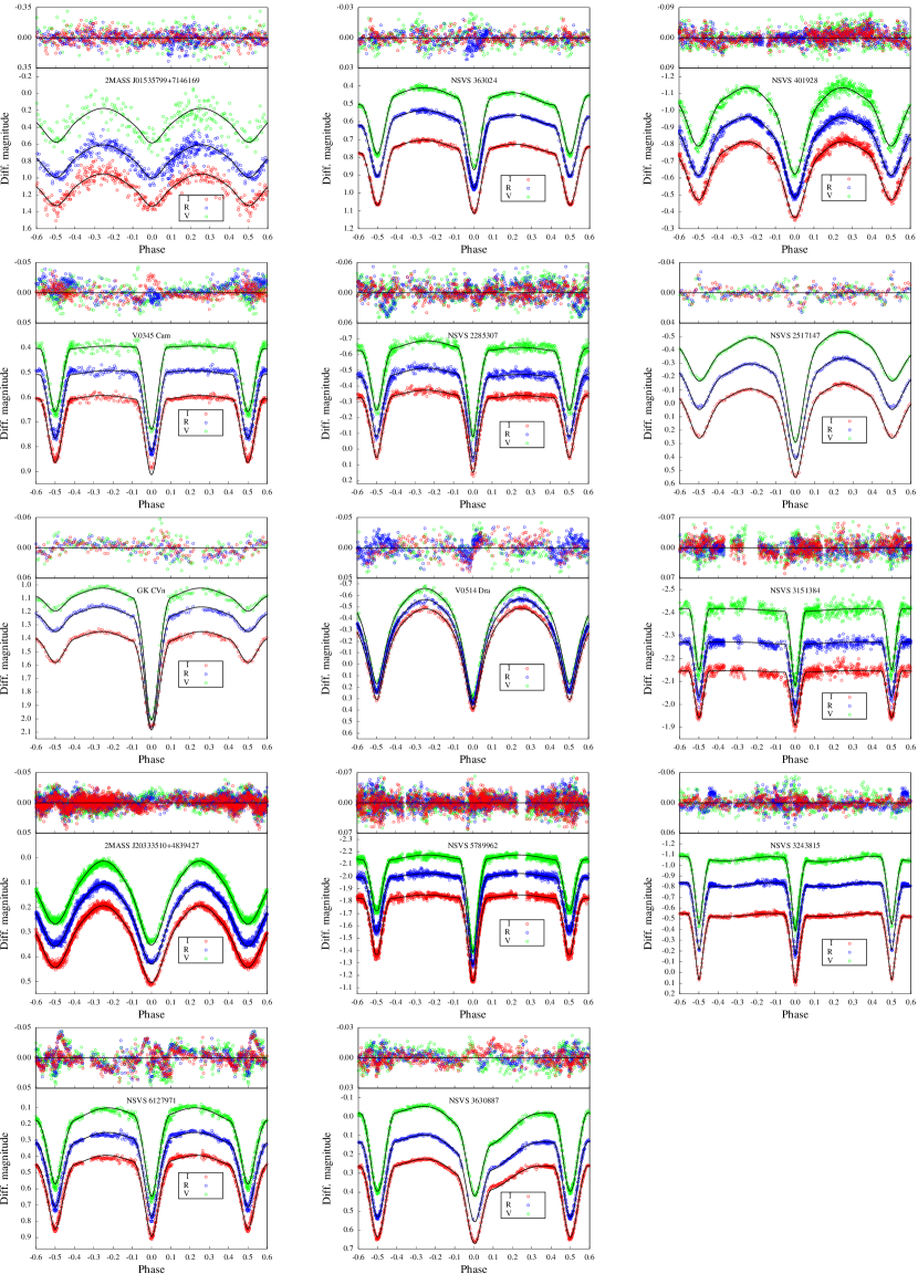
Figure 3.— Light curves. Final fit according to PHOEBE.

Table 7Masses, radii and orbital periods of double-lined low-mass binary components which uncertainties of masses and radii are less than 5 %.

System	Mass	Radius	Period	References
	[$M_{\astrosun}$]	[$R_{\astrosun}$]	[d]
BX Tri A	0.51 (2)	0.55 (1)	0.192	1
NSVS 01031772 A	0.5428 (27)	0.5260 (28)	0.368	2
NSVS 01031772 B	0.4982 (25)	0.5088 (30)	0.368	2
NGC2204-S892 A	0.733 (5)	0.719 (14)	0.452	3
NGC2204-S892 B	0.662 (5)	0.680 (17)	0.452	3
GU Boo A	0.6101 (64)	0.627 (16)	0.489	4, 5
GU Boo B	0.5995 (64)	0.624 (16)	0.489	4, 5
NSVS 02502726 A	0.714 (19)	0.645 (6)	0.560	6
NSVS 02502726 B	0.347 (12)	0.501 (5)	0.560	6
RT And B	0.907 (17)	0.906 (11)	0.629	4, 7
MG1-1819499 A	0.557 (1)	0.569 (25)	0.630	8
MG1-1819499 B	0.535 (1)	0.500 (17)	0.630	8
CG Cyg A	0.941 (14)	0.893 (12)	0.631	4, 7
CG Cyg B	0.814 (13)	0.838 (11)	0.631	4, 7
GSC 08814-01026 A	0.833 (17)	0.845 (12)	0.702	1
GSC 08814-01026 B	0.703 (13)	0.718 (17)	0.702	1
GJ 3236 A	0.375 (16)	0.3829 (57)	0.771	9
YY Gem A	0.5992 (47)	0.6194 (57)	0.814	4, 10
YY Gem B	0.5992 (47)	0.6194 (57)	0.814	4, 10
MG1-116309 A	0.567 (2)	0.552 (17)	0.827	8
MG1-116309 B	0.532 (2)	0.532 (12)	0.827	8
UV Psc A	0.9829 (77)	1.110 (23)	0.861	4, 11
UV Psc B	0.7644 (45)	0.835 (18)	0.861	4, 11
GSC 04894-02310 A	0.771 (33)	0.772 (12)	0.897	1
GSC 04894-02310 B	0.768 (33)	0.769 (13)	0.897	1
AE For A	0.6314 (35)	0.67 (3)	0.918	12
AE For B	0.6197 (34)	0.63 (3)	0.918	12
CM Dra A	0.23102 (89)	0.2534 (19)	1.268	4, 13
CM Dra B	0.21409 (83)	0.2398 (18)	1.268	4, 13
IM Vir A	0.981 (12)	1.061 (16)	1.309	14
IM Vir B	0.6644 (48)	0.681 (13)	1.309	14
BD-15 2429 A	0.7029 (45)	0.694 (9)	1.528	1
BD-15 2429 B	0.6872 (49)	0.699 (13)	1.528	1
MG1-506664 A	0.584 (2)	0.560 (5)	1.548	8
MG1-506664 B	0.544 (2)	0.513 (9)	1.548	8
MG1-78457 A	0.527 (2)	0.505 (15)	1.586	8
MG1-78457 B	0.491 (1)	0.471 (16)	1.586	8
TYC 4749-560-1 A	0.8338 (36)	0.848 (5)	1.622	1
TYC 4749-560-1 B	0.8280 (40)	0.833 (5)	1.622	1
MG1-646680 A	0.499 (2)	0.457 (10)	1.638	8
MG1-646680 B	0.443 (2)	0.427 (8)	1.638	8
MG1-2056316 A	0.469 (2)	0.441 (4)	1.723	8
MG1-2056316 B	0.382 (1)	0.374 (4)	1.723	8
RX J0239.1-1028 A	0.7300 (90)	0.7410 (40)	2.072	15, 16
RX J0239.1-1028 B	0.6930 (60)	0.7030 (20)	2.072	15, 16
FL Lyr B	0.958 (12)	0.962 (28)	2.178	4, 17
ZZ UMa B	0.9691 (48)	1.1562 (96)	2.299	4
V1061 Cyg Ab	0.9315 (68)	0.974 (20)	2.347	4, 18
V1236 Tau A	0.787 (12)	0.788 (15)	2.588	19
V1236 Tau B	0.770 (9)	0.817 (10)	2.588	19
CU Cnc A	0.4349 (12)	0.4323 (55)	2.771	4, 20
CU Cnc B	0.39922 (89)	0.3916 (94)	2.771	4, 20
G 179-55 A	0.2576 (85)	0.2895 (68)	3.550	9, 21
G 179-55 B	0.2585 (80)	0.2895 (68)	3.550	9, 21
T-Cyg1-12664 A	0.680 (21)	0.613 (7)	4.129	1
V636 Cen B	0.8545 (30)	0.8300 (43)	4.284	4
V818 Tau A	1.0591 (62)	0.900 (16)	5.609	10
V818 Tau B	0.7605 (62)	0.768 (10)	5.609	10
HS Aur A	0.898 (19)	1.004 (24)	9.815	4, 17
HS Aur B	0.877 (17)	0.874 (24)	9.815	4, 17
RW Lac B	0.8688 (40)	0.9638 (40)	10.369	4, 22
V568 Lyr B	0.8273 (42)	0.7679 (64)	14.470	4
KIC 6131659 A	0.922 (7)	0.8800 (28)	17.528	23
KIC 6131659 B	0.685 (5)	0.6395 (61)	17.528	23
FBS 1109+767 A	0.3951 (22)	0.3814 (31)	41.032	24
FBS 1109+767 B	0.2749 (11)	0.3001 (45)	41.032	24

References: 1 Çakırlı et al. (2013), 2 López-Morales et al. (2006), 3 Rozyczka et al. (2009), 4 Torres et al. (2010), 5 López-Morales & Ribas (2005), 6 Çakırlı et al. (2009), 7 Popper (1994), 8 Kraus et al. (2011), 9 Irwin et al. (2009), 10 Torres & Ribas (2002), 11 Popper (1997), 12 Rozyczka et al. (2013), 13 Morales et al. (2009b), 14 Morales et al. (2009a), 15 López-Morales & Shaw (2007), 16 Feiden & Chaboyer (2012), 17 Popper et al. (1986), 18 Torres et al. (2006), 19 Bayless & Orosz (2006), 20 Ribas (2003), 21 Hartman et al. (2011), 22 Lacy et al. (2005), 23 Bass et al. (2012), 24 Irwin et al. (2011)

Appendix A Observation log

Table 8Information about observations.

System	From	To	$N$	Aperture	Comparison star
	[d/m/y]	[d/m/y]	[I/R/V]	[arc sec]
2MASS J01535799+7146169	31/01/15	25/07/16	375/483/208	1.4	2MASS J01535745+7146059
NSVS 363024	31/01/15	25/07/16	295a/435a/307a	3.7	2MASS J01545478+7139110
NSVS 401928	04/04/15	17/08/16	620/800/606	3.7	2MASS J03261195+6956176
V0345 Cam	17/04/15	19/01/16	317/358/311	3.7	2MASS J04263015+6917324
NSVS 2285307	25/02/15	09/12/15	517/559/551	3.7	2MASS J06083785+5830425
NSVS 2517147	30/01/15	16/02/15	131/135/133	4.9	2MASS J09195939+5711028
GK CVn	20/04/16	15/09/16	135/125/136	2.8	2MASS J14011012+3346159
V0514 Dra	07/03/15	03/06/15	219/485/226	3.7	2MASS J17210185+6953376
NSVS 3151384	10/05/15	19/01/16	660/648/686	7.7	2MASS J20195374+6536570
2MASS J20333510+4839427	28/09/15	13/11/16	1514/1359/1393	2.8	2MASS J20332212+4843435
NSVS 5789962	28/09/15	08/11/16	1264/1226/1303	3.7	2MASS J20334670+4846449
NSVS 3243815	26/02/15	26/01/16	530/650/542	2.8	2MASS J20382276+5802417
NSVS 6127971	24/09/15	17/08/16	445/440/455	3.7	2MASS J22501858+3843502
NSVS 3630887	02/09/15	05/10/15	413/353/409	4.9	2MASS J23554892+3907373
a Does not contain data with evolved spot.

Appendix B Summary of observations

Table 9Summary of observations. Exp. time in format I/R/V (zero means we do not have any data from this filter).

System	Date	Exp. time	Weather condition
		[s]
2MASS J01535799+7146169	31/01/15	0/30/0	cirrus
	27/08/15	30/30/30	clouds all the time, Moon
	02/09/15	30/30/30	clouds, Moon, high humidity, fog
	04/09/15	45/30/45	clouds, Moon
	19/01/16	30/30/30	clear, Moon
	24/02/16	30/30/30	clear
	25/07/16	30/30/30	some clouds, Moon
NSVS 363024	31/01/15	0/30/0	cirrus
	27/08/15	30/30/30	clouds all the time, Moon
	02/09/15	30/30/30	clouds, Moon, high humidity, fog
	04/09/15	45/30/45	clouds, Moon
	19/01/16	30/30/30	clear, Moon
	24/02/16	30/30/30	clear
	25/07/16	30/30/30	some clouds, Moon
NSVS 401928	04/04/15	0/60/0	clear
	18/11/15	30/30/30	some clouds, windy
	09/12/15	30/30/30	clouds, high humidity
	19/01/16	30/30/30	clouds, Moon
	26/01/16	30/30/30	clouds, Moon, high humidity
	10/02/16	30/30/30	clouds
	24/02/16	30/30/30	clouds, Moon
	25/05/16	30/30/30	clouds
	18/08/16	30/30/30	clear, Moon
V0345 Cam	17/04/15	0/45/0	clear
	04/09/15	45/45/45	clouds, Moon
	01/10/15	45/45/45	clear, Moon
	24/10/15	60/60/60	cirrus, Moon
	03/11/15	30/20/40	mostly clear, Moon
	19/01/16	30/20/40	clouds, Moon
NSVS 2285307	26/11/14	0/60/90	some clouds
	25/02/15	60/60/60	clouds, Moon
	02/03/15	60/60/60	clouds, Moon
	16/03/15	60/60/60	clouds
	13/04/15	60/60/60	somewhat cloudy
	22/04/15	60/60/60	some clouds
	27/10/15	60/60/60	clear, Moon
	03/11/15	45/30/45	clear
	18/11/15	45/30/45	clouds, windy
	24/11/15	45/30/45	thin cirrus
	09/12/15	45/30/45	clear, very high humidity
NSVS 2517147	30/01/15	0/60/0	cloudsa
	16/02/15	60/60/60	clear
GK CVn	20/04/16	80/80/80	clear, Moon
	28/08/16	80/80/80	thin cirrus
	15/09/16	0/60/0	clear, Moon
V0514 Dra	07/03/15	0/30/0	clear
	13/04/15	30/30/30	somewhat cloudy
	29/04/15	0/30/0	cirrus, Moon
	04/05/15	30/30/30	clouds, Moon
	03/06/15	30/30/30	clear
NSVS 3151384	10/05/15	0/60/0	clear
	03/06/15	45/45/45	clear
	02/07/15	45/45/45	clear, Moon
	29/07/15	45/45/45	somewhat cloudy, Moon
	30/07/15	45/45/45	some clouds, Moon
	31/07/15	45/45/45	clouds, Moon
	03/08/15	45/45/45	clear, Moon
	05/08/15	45/30/45	clouds, Moon
	27/10/15	45/30/45	clear, Moon
	03/11/15	30/30/45	clear
	19/01/16	30/30/45	clouds
2MASS J20333510+4839427	28/09/15	30/30/30	clouds, Moon
	24/11/15	30/30/30	clear, Moon
	24/04/16	30/30/30	some clouds, Moon
	25/05/16	30/30/30	clear, Moon
	06/06/16	30/30/30	clear
	21/06/16	30/30/30	clear, Moon
	29/06/16	30/20/30	clear
	25/07/16	30/20/30	some clouds
	31/08/16	30/20/30	clear
	15/09/16	30/20/30	clear, Moon
	13/11/16	30/20/30	clear, Moon
NSVS 5789962	28/09/15	30/30/30	clouds, Moon
	24/11/15	30/30/30	clear, Moon
	24/04/16	30/30/30	some clouds, Moon
	25/05/16	30/30/30	clear, Moon
	06/06/16	30/30/30	clear
	21/06/16	30/30/30	clear, Moon
	29/06/16	30/20/30	clear
	25/07/16	30/20/30	some clouds
	31/08/16	30/20/30	clear
	15/09/16	30/20/30	clear, Moon
NSVS 3243815	26/02/15	0/45/0	clear, Moon
	10/04/15	0/45/0	clear
	03/07/15	45/45/45	clear
	04/07/15	45/45/45	cirrus
	07/07/15	45/45/45	clear
	03/08/15	45/45/45	clear, Moon
	25/08/15	45/45/45	clouds, later clear, Moon
	27/08/15	45/45/45	clouds, Moon
	20/09/15	45/45/45	clouds
	24/11/15	45/45/45	thin cirrus, Moon
	19/01/16	45/45/45	clouds, Moon
	26/01/16	45/45/45	some clouds, Moon
NSVS 6127971	24/09/15	45/45/45	clouds, Moon
	30/09/15	45/45/60	clear, Moon
	18/11/15	30/30/30	clouds, windy
	19/01/16	30/30/30	clear, Moon
	06/06/16	30/30/30	clear
	29/61/16	30/30/30	clear
	25/07/16	30/30/30	some clouds
	17/08/16	30/30/30	clear, Moon
NSVS 3630887	02/09/15	30/30/30	clouds, high humidity, Moon, fog
	09/09/15	30/30/30	high humidity
	20/09/15	30/30/30	clouds
	05/10/15	45/45/45	clouds
a The data were used for deriving the mid-eclipse time.

Appendix C Tables of minima

Table 10Times of mid-eclipses. Ephemerides were adopted from Table 3.

System	Time of eclipse	p/s	Epoch
	[HJD-2400000]
2MASS J01535799+7146169	57054.450 (34)	p	-774.0
	57262.3092 (31)	s	-22.5
	57262.5842 (22)	s	-21.5
	57268.5285 (19)	p	0.0
	57270.4681 (28)	p	7.0
	57443.3381 (43)	p	632.0
	57595.612 (14)	s	1182.5
NSVS 363024	57054.47924 (50)	p	-494.0
	57262.6333 (75)	p	-13.5
	57268.48295 (19)	p	0.0
	57270.43109 (26)	s	4.5
	57407.3253 (96)	s	320.5
	57443.2815 (16)	s	403.5
	57595.5523 (16)	p	755.0
NSVS 401928	57117.41825 (23)	p	0.0
	57345.1854 (29)	s	393.5
	57407.4091 (25)	p	501.0
	57414.36165 (99)	p	513.0
	57414.6500 (17)	s	513.5
	57429.4133 (28)	p	539.0
	57443.30108 (77)	p	563.0
	57443.5921 (13)	s	563.5
	57618.40194 (26)	s	865.5
V0345 Cam	57130.3872 (12)	p	-370.0
	57270.60216 (90)	s	-59.5
	57297.47183 (17)	p	0.0
	57320.2770 (55)	s	50.5
	57320.5016 (45)	p	51.0
	57330.66337 (23)	s	73.5
	57407.43340 (62)	s	243.5
NSVS 2285307	56988.2942 (25)	s	-277.5
	57079.4148 (11)	s	-86.5
	57084.2634 (11)	p	-79.0
	57135.31620 (42)	p	0.0
	57165.3655 (18)	s	46.5
	57330.48189 (26)	p	302.0
	57351.48411 (19)	s	334.5
	57366.6703 (22)	p	358.0
NSVS 2517147	57053.3827 (73)	s	-38.5
	57070.35638 (33)	s	-0.5
	57070.58140 (20)	p	0.0
GK CVn	57499.36503 (23)	s	-0.5
	57499.56797 (19)	p	0.0
	57647.2404 (12)	p	368.0
V0514 Dra	57089.41835 (34)	p	0.0
	57126.49623 (76)	p	118.0
	57126.65323 (87)	s	118.5
	57142.36430 (17)	s	168.5
	57147.39192 (54)	s	184.5
	57177.39940 (39)	p	280
NSVS 3151384	57206.42061 (23)	p	0.0
	57233.3027 (39)	s	21.5
	57234.55858 (40)	s	22.5
	57323.34199 (53)	s	93.5
	57330.22016 (30)	p	99.0
2MASS J20333510+4839427	57294.33255 (89)	s	-385.5
	57351.2105 (44)	s	-280.5
	57503.4376 (10)	s	0.5
	57546.5019 (27)	p	80.0
	57561.40109 (55)	s	107.5
	57569.5273 (24)	s	122.5
	57595.5280 (31)	s	170.5
	57632.36678 (66)	s	238.5
	57632.6349 (22)	p	239.0
	57647.5358 (12)	s	266.5
	57706.31349 (69)	p	375.0
NSVS 5789962	57294.43858 (30)	p	0.0
	57351.2336 (41)	p	39.0
	57503.42106 (29)	s	143.5
	57546.38177 (16)	p	173.0
	57632.30643 (10)	p	232.0
	57647.59699 (26)	s	242.5
NSVS 3243815	57207.3531 (70)	s	-36.5
	57238.46067 (28)	s	-0.5
	57260.49427 (34)	p	25.0
	57286.41699 (30)	p	55.0
	57351.22274 (95)	p	130.0
	57407.3884 (56)	p	195.0
	57414.3018 (12)	p	203.0
NSVS 6127971	57290.52442 (93)	p	-11.0
	57296.48408 (66)	p	0.0
	57407.26738 (39)	s	204.5
	57546.49165 (22)	s	461.5
	57569.51647 (30)	p	504.0
	57618.54307 (41)	s	594.5
NSVS 3630887	57268.40597 (56)	s	-15.5
	57275.30876 (20)	s	-0.5
	57275.54046 (25)	p	0.0
	57286.35337 (26)	s	23.5
	57301.5403 (13)	s	56.5

References

- Bass et al. (2012) Bass, G., Orosz, J. A., Welsh, W. F., et al. 2012, ApJ, 761, 157
- Bayless & Orosz (2006) Bayless, A. J., & Orosz, J. A. 2006, ApJ, 651, 1155
- Berdyugina (2005) Berdyugina, S. V. 2005, Living Reviews in Solar Physics, 2, 8
- Bessell (1990) Bessell, M. S. 1990, PASP, 102, 1181
- Çakırlı et al. (2009) Çakırlı, Ö., İbanoǧlu, C., & Güngör, C. 2009, NewA, 14, 496
- Çakırlı et al. (2013) Çakırlı, Ö., İbanoǧlu, C., & Sipahi, E. 2013, MNRAS, 429, 85
- Chabrier et al. (2007) Chabrier, G., Gallardo, J., & Baraffe, I. 2007, A&A, 472, L17
- Coughlin et al. (2011) Coughlin, J. L., López-Morales, M., Harrison, T. E., Ule, N., & Hoffman, D. I. 2011, AJ, 141, 78
- Cutri et al. (2003) Cutri, R. M., Skrutskie, M. F., van Dyk, S., et al. 2003, VizieR Online Data Catalog, 2246, 0
- Eker et al. (2015) Eker, Z., Soydugan, F., Soydugan, E., et al. 2015, AJ, 149, 131
- Feiden & Chaboyer (2012) Feiden, G. A., & Chaboyer, B. 2012, ApJ, 757, 42
- Graczyk (2003) Graczyk, D. 2003, MNRAS, 342, 1334
- Hartman et al. (2011) Hartman, J. D., Bakos, G. Á., Noyes, R. W., et al. 2011, AJ, 141, 166
- Hoffman et al. (2008) Hoffman, D. I., Harrison, T. E., Coughlin, J. L., et al. 2008, AJ, 136, 1067
- Irwin et al. (2009) Irwin, J., Charbonneau, D., Berta, Z. K., et al. 2009, ApJ, 701, 1436
- Irwin et al. (2011) Irwin, J. M., Quinn, S. N., Berta, Z. K., et al. 2011, ApJ, 742, 123
- Kraus et al. (2011) Kraus, A. L., Tucker, R. A., Thompson, M. I., Craine, E. R., & Hillenbrand, L. A. 2011, ApJ, 728, 48
- Kroupa et al. (2013) Kroupa, P., Weidner, C., Pflamm-Altenburg, J., et al. 2013, The Stellar and Sub-Stellar Initial Mass Function of Simple and Composite Populations, ed. T. D. Oswalt & G. Gilmore, 115
- Künstler et al. (2015) Künstler, A., Carroll, T. A., & Strassmeier, K. G. 2015, A&A, 578, A101
- Lacy et al. (2005) Lacy, C. H. S., Torres, G., Claret, A., & Vaz, L. P. R. 2005, AJ, 130, 2838
- López-Morales et al. (2006) López-Morales, M., Orosz, J. A., Shaw, J. S., et al. 2006, ArXiv Astrophysics e-prints, astro-ph/0610225
- López-Morales & Ribas (2005) López-Morales, M., & Ribas, I. 2005, ApJ, 631, 1120
- López-Morales & Shaw (2007) López-Morales, M., & Shaw, J. S. 2007, in Astronomical Society of the Pacific Conference Series, Vol. 362, The Seventh Pacific Rim Conference on Stellar Astrophysics, ed. Y. W. Kang, H.-W. Lee, K.-C. Leung, & K.-S. Cheng, 26
- Morales et al. (2011) Morales, J. C., Ribas, I., & Jordi, C. 2011, in Astronomical Society of the Pacific Conference Series, Vol. 448, 16th Cambridge Workshop on Cool Stars, Stellar Systems, and the Sun, ed. C. Johns-Krull, M. K. Browning, & A. A. West, 99
- Morales et al. (2009a) Morales, J. C., Torres, G., Marschall, L. A., & Brehm, W. 2009a, ApJ, 707, 671
- Morales et al. (2009b) Morales, J. C., Ribas, I., Jordi, C., et al. 2009b, ApJ, 691, 1400
- Motl (2011) Motl, D. 2011, Muniwin
- Nikolaev et al. (2000) Nikolaev, S., Weinberg, M. D., Skrutskie, M. F., et al. 2000, AJ, 120, 3340
- Paxton (2004) Paxton, B. 2004, PASP, 116, 699
- Pecaut & Mamajek (2013) Pecaut, M. J., & Mamajek, E. E. 2013, ApJS, 208, 9
- Popper (1994) Popper, D. M. 1994, AJ, 108, 1091
- Popper (1997) —. 1997, AJ, 114, 1195
- Popper et al. (1986) Popper, D. M., Lacy, C. H., Frueh, M. L., & Turner, A. E. 1986, AJ, 91, 383
- Prša & Zwitter (2005) Prša, A., & Zwitter, T. 2005, ApJ, 628, 426
- Ribas (2003) Ribas, I. 2003, A&A, 398, 239
- Rozyczka et al. (2009) Rozyczka, M., Kaluzny, J., Pietrukowicz, P., et al. 2009, AcA, 59, 385
- Rozyczka et al. (2013) Rozyczka, M., Pietrukowicz, P., Kaluzny, J., et al. 2013, MNRAS, 429, 1840
- Schwarz (1978) Schwarz, G. 1978, Annals of Statistics, 6, 461
- Spada et al. (2013) Spada, F., Demarque, P., Kim, Y.-C., & Sills, A. 2013, ApJ, 776, 87
- Stassun et al. (2014) Stassun, K. G., Feiden, G. A., & Torres, G. 2014, NewAR, 60, 1
- Torres et al. (2010) Torres, G., Andersen, J., & Giménez, A. 2010, A&A Rev., 18, 67
- Torres et al. (2006) Torres, G., Lacy, C. H., Marschall, L. A., Sheets, H. A., & Mader, J. A. 2006, ApJ, 640, 1018
- Torres & Ribas (2002) Torres, G., & Ribas, I. 2002, ApJ, 567, 1140
- van Hamme (1993) van Hamme, W. 1993, AJ, 106, 2096
- Wilson & Devinney (1971) Wilson, R. E., & Devinney, E. J. 1971, ApJ, 166, 605