Uniform bounds and asymptotics of Generalized Gegenbauer functions of fractional degree

Abstract.

The generalised Gegenbauer functions of fractional degree (GGF-Fs), denoted by ${}^{r\!}G^{(\lambda)}_{\nu}(x)$ (right GGF-Fs) and ${}^{l}G^{(\lambda)}_{\nu}(x)$ (left GGF-Fs) with $x\in(-1,1),$ $\lambda>-1/2$ and real $\nu\geq 0,$ are special functions (usually non-polynomials), which are defined upon the hypergeometric representation of the classical Gegenbauer polynomial by allowing integer degree to be real fractional degree. Remarkably, the GGF-Fs become indispensable for optimal error estimates of polynomial approximation to singular functions, and have intimate relations with several families of nonstandard basis functions recently introduced for solving fractional differential equations. However, some properties of GGF-Fs, which are important pieces for the analysis and applications, are unknown or under explored. The purposes of this paper are twofold. The first is to show that for $\lambda,\nu>0$ and $x=\cos\theta$ with $\theta\in(0,\pi),$

$$(\sin\theta)^{\lambda}\,{}^{r\!}G_{\nu}^{(\lambda)}(\cos\theta)=\frac{2^{\lambda}\Gamma(\lambda+1/2)}{\sqrt{\pi}{(\nu+\lambda)^{\lambda}}}\,{\cos((\nu+\lambda)\theta-\lambda\pi/2)}+{\mathcal{R}}_{\nu}^{(\lambda)}(\theta),$$

and derive the precise expression of the “residual” term ${\mathcal{R}}_{\nu}^{(\lambda)}(\theta).$ With this at our disposal, we obtain the bounds of GGF-Fs uniform in $\nu.$ Under an appropriate weight function, the bounds are uniform for $\theta\in[0,\pi]$ as well. Moreover, we can study the asymptotics of GGF-Fs with large fractional degree $\nu.$ The second is to present miscellaneous properties of GGF-Fs for better understanding of this family of useful special functions.

1. Introduction

Undoubtedly, polynomial approximation theory occupies a central place in algorithm development and numerical analysis of perhaps most of computational methods. Indeed, one finds numerous approximation results in various senses documented in a large volume of literature, which particularly include orthogonal polynomial approximation results related to spectral methods and $hp$-version finite element methods (see, e.g., [4, 20, 24, 21] and the references therein). Typically, such results are established in Jacobi-weighted Sobolev spaces with integral-order regularity exponentials (see, e.g., [21]), or weighted Besov spaces with fractional regularity exponentials using the notion of space interpolation (see, e.g., [5, 6, 7]). In a very recent work [13], we introduced a new framework of fractional Sobolev-type spaces involving Riemann-Liouville (RL) fractional integrals and derivatives in the study of polynomial approximation to singular functions. Such spaces are naturally arisen from exact representations of orthogonal polynomial expansion coefficients, and could best characterize the fractional differentiability/regularity, leading to optimal error estimates. A very important piece of the puzzle therein is the so-called GGF-Fs that generalize the classical Gegenbauer polynomials of integer degree to functions of fractional degree. It is noteworthy that the GGF-Fs can be generalized by different means, e.g., the Rodrigues’ formula and hypergeometric function representation. For instance, the right GGF-F: ${}^{r\!}G^{(\lambda)}_{\nu}(x)$ can be viewed as special $g$-Jacobi functions (see Mirevski et al [15]), defined by replacing the integer-order derivative in the Rodrigues’ formula of the Jacobi polynomials by the RL fractional derivative. However, both the definition and derivation of some properties in [15] have flaws (see Remark 4.1). On the other hand, the Handbook [17, (15.9.15)] listed ${}^{r\!}G^{(\lambda)}_{\nu}(x)$ but without presented any of their properties. Interestingly, as pointed out in [13], the GGF-Fs have a direct bearing on Jacobi polyfractonomial (cf. [28]) and generalised Jacobi functions (cf. [10, 8]) recently introduced in developing efficient spectral methods for fractional differential equations. It is also noteworthy that the seminal work of Gui and Babuška [9] on $hp$-estimates of Legendre approximation of singular functions essentially relied on some non-classical Jacobi polynomials with the parameter $\alpha$ or $\beta<-1,$ which turned out closely related to GGF-Fs. In a nutshell, the GGF-Fs (and more generally the generalised Jacobi functions of fractional degree) can be of great value for numerical analysis and computational algorithms, but many of their properties are still under explored.

It is known that the study of asymptotics has been a longstanding subject of special functions and their far reaching applications (see, e.g., [16, 23, 17]). Most of the asymptotic results of classical orthogonal polynomials can be found in the books [22, 17], and are reported in the review papers [14, 26, 27] in more general senses. We highlight that the asymptotic formulas of the hypergeometric function: ${}_{2}F_{1}(a-\mu,b+\mu;c;(1-z)/2)$ in terms of Bessel functions for large $\mu,$ were derived in Jones [11] following the idea of Olver [16] using differential equations, where the representations with fewer restrictions on the parameters different from those in Watson [25] could be obtained. Farid Khwaja and Olde Daalhuis [12] discussed asymptotics of ${}_{2}F_{1}(a-e_{1}\mu,b+e_{2}\mu;c+e_{3}\mu;(1-z)/2)$ with $e_{j}=0,\pm 1,j=1,2,3$ in terms of Bessel functions by using the contour integrals.

One of the main objectives of this paper is to derive the uniform bounds for the GGF-Fs, which are valid for real degree $\nu>0$ with fixed $\lambda,$ and also for all $\theta\in[0,\pi]$ but with a suitable weight function to absorb the singularities at the endpoints. As such, we can obtain the asymptotic formulas for large degree $\nu,$ and some other useful estimates of the GGF-Fs. Our delicate analysis is based on an integral representation from a very useful fractional integral formula in [13] (see (2.7) and Lemma 2.1). In fact, the Watson’s Lemma and asymptotic analysis for Legendre polynomials (cf. [16]) indeed cast light on our study. It is important to point out the GGF-Fs are defined as hypergeometric functions with special parameters (see Definition 2.1), so some asymptotic results follow from [11, 12] for large parameters in terms of Bessel functions. However, we intend to derive the results uniform for the degree and the variable, and the estimates for large parameters are directly consequences. In other words, our study can lead to different and more explicitly informative estimates. As such, the results herein can offer useful tools for analysis of polynomial approximation and applications of this family of special functions. A second purpose of this paper is to present various properties of GGF-Fs. These particularly include singular behaviors of GGF-Fs in the vicinity of the endpoints, and useful fractional calculus formulas.

The paper is organized as follows. In Section 2, we first introduce the definition of GGF-Fs, and then present the main results. We then provide their proofs in Section 3. In the last section, we present assorted properties of GGF-Fs for better understanding of this family of special functions.

2. Main result and its proof

2.1. Generalised Gegenbauer functions of fractional degree

Different from Mirevski et al [15], we follow [13] to define two types of GGF-Fs by the hypergeometric function.

Definition 2.1.

For real $\lambda>-1/2,$ we define the right GGF-F on $(-1,1)$ of real degree $\nu\geq 0$ as

$${}^{r\!}G_{\nu}^{(\lambda)}(x)=\,{}_{2}F_{1}\Big{(}\!\!-\nu,\nu+2\lambda;\lambda+\frac{1}{2};\frac{1-x}{2}\Big{)}=1+\sum_{j=1}^{\infty}\frac{(-\nu)_{j}(\nu+2\lambda)_{j}}{j!\;(\lambda+1/2)_{j}}\Big{(}\frac{1-x}{2}\Big{)}^{j},$$ (2.1)

and the left GGF-F of real degree $\nu\geq 0$ as

$$\begin{split}{}^{l}G_{\nu}^{(\lambda)}(x)=(-1)^{[\nu]}\,{}_{2}F_{1}\Big{(}\!\!-\nu,\nu+2\lambda;\lambda+\frac{1}{2};\frac{1+x}{2}\Big{)}=(-1)^{[\nu]}\,{}^{r\!}G_{\nu}^{(\lambda)}(-x),\end{split}$$ (2.2)

where $[\nu]$ is the largest integer $\leq\nu,$ and the Pochhammer symbol: $(a)_{j}=a(a+1)\cdots(a+j-1).$

In the above, the hypergeometric function is a power series given by

$${}_{2}F_{1}(a,b;c;z)=1+\sum_{j=1}^{\infty}\frac{(a)_{j}(b)_{j}}{(c)_{j}}\frac{z^{j}}{j!},$$ (2.3)

where $a,b,c$ are real, and $-c\not\in{\mathbb{N}}:=\{1,2,\cdots\}$ (see, e.g., [3]).

Note that if $\nu=n\in{\mathbb{N}}_{0}:=\{0\}\cup{\mathbb{N}}$, we have

$${}^{r\!}G_{n}^{(\lambda)}(x)={}^{l}G_{n}^{(\lambda)}(x)=G_{n}^{(\lambda)}(x)=\frac{P_{n}^{(\lambda-1/2,\lambda-1/2)}(x)}{P_{n}^{(\lambda-1/2,\lambda-1/2)}(1)},\;\;\;\lambda>-\frac{1}{2},$$ (2.4)

where $P_{n}^{(\alpha,\beta)}(x)$ is the classical Jacobi polynomial as defined in Szegö [22]. For $\lambda=1/2,$ the right GGF-F turns to be the Legendre function (cf. [23]): ${}^{r}G_{\nu}^{(1/2)}(x)=P_{\nu}(x).$ For $\lambda=0,$ we have

$${}^{r\!}G_{\nu}^{(0)}(x)={}^{r\!}G_{\nu}^{(0)}(\cos\theta)=\cos(\nu\theta)=\cos(\nu\,{\rm arccos}x):=T_{\nu}(x),$$ (2.5)

thanks to the property (cf. [1, (15.1.17)]):

$${}_{2}F_{1}(-a,a,1/2\,;\,\sin^{2}t)=\cos(2at),\quad a,t\in{\mathbb{R}}:=(-\infty,\infty).$$ (2.6)

Remark 2.1.

The GGF-Fs ${}^{r\!}G_{n-\lambda+1/2}^{(\lambda)}(x)$ and ${}^{l}G_{n-\lambda+1/2}^{(\lambda)}(x)$ with integer $n$ up to some constant multiple, coincide with some nonstandard singular basis functions introduced in [28, 8] for accurate solution of fractional differential equations.

Inherited from the Bateman’s fractional integral formula for hypergeometric functions (cf. [3, P. 313]), we can derive the following very useful formula (cf. [13, Thm. 3.1]): for $\lambda>-1/2,$ and real $\nu\geq s\geq 0,$

$$\begin{split}{}_{x}I_{1}^{s}\big{\{}(1-x^{2})^{\lambda-1/2}\,{}^{r\!}G_{\nu}^{(\lambda)}(x)\big{\}}&=\frac{1}{\Gamma(s)}\int_{x}^{1}\frac{(1-y^{2})^{\lambda-1/2}\,{}^{r\!}G_{\nu}^{(\lambda)}(y)}{(y-x)^{1-s}}dy\\ &=\frac{\Gamma(\lambda+1/2)}{2^{s}\Gamma(\lambda+s+1/2)}\,(1-x^{2})^{\lambda+s-1/2}\,{}^{r\!}G_{\nu-s}^{(\lambda+s)}(x),\;\;\end{split}$$ (2.7)

where ${}_{x}I_{1}^{s}$ is the right-sided RL fractional integral operator defined by

$${}_{x}I_{1}^{s}\,u(x)=\frac{1}{\Gamma(s)}\int_{x}^{1}\frac{u(y)}{(y-x)^{1-s}}dy.$$ (2.8)

Note that a similar formula is available for the left GGF-F ${}^{l}G_{\nu}^{(\lambda)}(x)$ but associated with the left-sided RL fractional integral.

Thanks to (2.7), we can derive the following formula crucial for the analysis.

Lemma 2.1.

For real $\nu,\lambda\geq 0,$ we have

$$(\sin\theta)^{2\lambda-1}\,{}^{r\!}G_{\nu}^{(\lambda)}(\cos\theta)=\frac{2^{\lambda}\,\Gamma(\lambda+1/2)}{\sqrt{\pi}\,\Gamma(\lambda)}\int^{\theta}_{0}\frac{\cos((\nu+\lambda)\phi)}{(\cos\phi-\cos\theta)^{1-\lambda}}\,d\phi,$$ (2.9)

for any $\theta\in(0,\pi).$

Proof.

From (2.5) and (2.7) with $\lambda=0$, we obtain immediately that for $\nu\geq s\geq 0,$

$$(1-x^{2})^{s-1/2}\,{}^{r\!}G_{\nu-s}^{(s)}(x)=\frac{2^{s}\,\Gamma(s+1/2)}{\sqrt{\pi}\,\Gamma(s)}\int_{x}^{1}\frac{1}{(y-x)^{1-s}}\frac{T_{\nu}(y)}{\sqrt{1-y^{2}}}\,dy.$$ (2.10)

Substituting $s$ and $\nu$ in the above identity by $\lambda$ and $\nu+\lambda,$ respectively, and using a change of variables: $x=\cos\theta$ and $y=\cos\phi,$ we derive (2.9) from (2.10) straightforwardly. ∎

Remark 2.2.

If $\lambda=1/2$ and $\nu=n,$ the identity (2.9) leads to the first Dirichlet-Mehler formula for the Legendre polynomial (cf. [23, (6.51)]):

$$P_{n}(\cos\theta)=\frac{\sqrt{2}}{\pi}\int_{0}^{\theta}\frac{\cos(n+1/2)\phi}{\sqrt{\cos\phi-\cos\theta}}\,d\phi,\;\;\;\;\;\theta\in(0,\pi),\;\;n\in{\mathbb{N}}_{0}.$$ (2.11)

One approach to obtain the asymptotic formula for Legendre polynomial with $n\to\infty$ is based on this formula, and the Watson’s lemma (cf. [16, P. 113]). This useful argument indeed sheds light on the study of GGF-Fs herein. However, we aim to study the behaviour of GGF-Fs uniform for all $\nu,$ so the route appears very different, delicate and more involved.

2.2. Main results

We first state the results, whose proofs are given in Section 3. Here, we just consider the right GGF-Fs, but thanks to (2.2), similar results can be obtained for the left counterparts.

Theorem 2.1.

For $\lambda>0$ and $\theta\in(0,\pi),$ we have

$$\begin{split}(\sin\theta)^{\lambda}\,{}^{r\!}G_{\nu}^{(\lambda)}(\cos\theta)=\frac{2^{\lambda}\Gamma(\lambda+1/2)}{\sqrt{\pi}{(\nu+\lambda)^{\lambda}}}\,{\cos((\nu+\lambda)\theta-\lambda\pi/2)}+{\mathcal{R}}_{\nu}^{(\lambda)}(\theta),\end{split}$$ (2.12)

where the “residual” term ${\mathcal{R}}_{\nu}^{(\lambda)}(\theta)$ with a representation given by (3.48), and there holds

$$|{\mathcal{R}}_{\nu}^{(\lambda)}(\theta)|\leq{\mathcal{S}}_{\nu}^{(\lambda)}(\theta),\quad\forall\,\theta\in(0,\pi).$$ (2.13)

Here, the bound ${\mathcal{S}}_{\nu}^{(\lambda)}(\theta)$ is given by

• for $0<\lambda\leq 2,\nu+\lambda>1$ and $\nu>0,$

  $$\begin{split}{\mathcal{S}}_{\nu}^{(\lambda)}(\theta)=\frac{\lambda|\lambda-1|2^{\lambda}\Gamma(\lambda+1/2)}{\sqrt{\pi}(\nu+\lambda-1)^{\lambda+1}}\Big{\{}|\cot\theta|+\frac{2}{3}\frac{\lambda+1}{\nu+\lambda-1}\Big{\}};\end{split}$$ (2.14)

• for $\lambda>2,\nu>\lambda-3$ and $\nu>0,$

  $$\begin{split}{\mathcal{S}}_{\nu}^{(\lambda)}(\theta)&=\frac{\lambda(\lambda-1)2^{3\lambda/2}\Gamma(\lambda+1/2)}{\sqrt{\pi}(\nu+1)^{\lambda+1}}\Big{\{}|\cot\theta|+\frac{2}{3}\frac{\lambda+1}{\nu+1}\\ &\quad+\frac{2^{2-\lambda}\Gamma(2\lambda-1)}{\Gamma(\lambda+1)}\frac{(\nu+1)^{\lambda+1}}{(\nu-\lambda+3)^{2\lambda-1}}|\cot\theta|^{\lambda-2}\Big{(}|\cot\theta|+\frac{2}{3}\frac{2\lambda-1}{\nu-\lambda+3}\Big{)}\Big{\}}.\end{split}$$ (2.15)

With Theorem 2.1 at our disposal, we next estimate the bound of ${\mathcal{S}}_{\nu}^{(\lambda)}(\theta)$, and characterize its explicit dependence of $\theta$ and decay rate in $\nu.$

Corollary 2.1.

For $\lambda>0,$ we have

$$\Big{|}(\sin\theta)^{\lambda}\,{}^{r\!}G_{\nu}^{(\lambda)}(\cos\theta)-\frac{2^{\lambda}\Gamma(\lambda+1/2)}{\sqrt{\pi}{(\nu+\lambda)^{\lambda}}}\,{\cos((\nu+\lambda)\theta-\lambda\pi/2)}\Big{|}\leq\frac{B^{(\lambda)}_{\nu}}{\nu^{\lambda+1}\sin\theta}\,,$$ (2.16)

where the constant $B^{(\lambda)}_{\nu}$ is given by

• for $0<\lambda\leq 2$ and $\nu+\lambda>1,$

  $${B}_{\nu}^{(\lambda)}=\frac{\lambda\,|\lambda-1|\,2^{\lambda}\,\Gamma(\lambda+1/2)}{\sqrt{\pi}}\,\frac{3\nu+5\lambda-1}{3(\nu+\lambda-1)}\,{\rm exp}\Big{(}\frac{1-\lambda^{2}}{\nu+\lambda-1}\Big{)},$$ (2.17)

  and the bound (2.16) holds for all $\theta\in(0,\pi);$

• for $\lambda>2$ and $\nu>\lambda-3,$ we have

  $$\begin{split}{B}_{\nu}^{(\lambda)}&=\frac{\lambda(\lambda-1)2^{3\lambda/2}\Gamma(\lambda+1/2)}{3\sqrt{\pi}}\bigg{\{}\frac{3\nu+2\lambda+5}{\nu+1}\\ &\quad+(c\pi)^{\lambda-2}\,\frac{\Gamma(2\lambda-1)}{\Gamma(\lambda+1)}\,\frac{3\nu+\lambda+7}{\nu-\lambda+3}\,{\rm exp}\Big{(}\frac{(2\lambda-5)(\lambda+1)}{\nu-\lambda+3}\Big{)}\bigg{\}},\end{split}$$ (2.18)

  and the bound (2.16) holds for all $\theta\in[c\nu^{-1},\pi-c\nu^{-1}]$ with $c$ being a fixed positive constant.

We provide the derivation of the above bounds right after the proof of Theorem 2.1. Note that in the second case: $\lambda>2,$ the bound is only available for $\theta\in[c\nu^{-1},\pi-c\nu^{-1}]$ with some fixed constant $c>0$. Indeed, the situation is reminiscent to the classical Gengenbauer polyomial with asymptotics only valid for $\theta\in[cn^{-1},\pi-cn^{-1}]$ with large $n,$ as we remark below.

Remark 2.3.

From (2.4) and Theorem 2.1, we obtain that for $\nu=n\in{\mathbb{N}},$

$$\begin{split}&(\sin\theta)^{\lambda}P_{n}^{(\lambda-1/2,\lambda-1/2)}(\cos\theta)=(\sin\theta)^{\lambda}\,P_{n}^{(\lambda-1/2,\lambda-1/2)}(1)\,G_{n}^{(\lambda)}(\cos\theta)\\ &\quad=\frac{2^{\lambda}\Gamma(n+\lambda+1/2)}{\sqrt{\pi}\,n!\,{(n+\lambda)^{\lambda}}}\,{\cos((n+\lambda)\theta-\lambda\pi/2)}+\frac{\Gamma(n+\lambda+1/2)}{\Gamma(\lambda+1/2)n!}{\mathcal{R}}_{n}^{(\lambda)}(\theta).\end{split}$$ (2.19)

Then from Corollary 2.1, we can derive the bounds uniform for $n.$ In fact, we can recover the asymptotic formula for the classical Gegenbauer polynomial with large $n$ (cf. [22, Thm 8.21.13]):

$$(\sin\theta)^{\lambda}P_{n}^{(\lambda-1/2,\lambda-1/2)}(\cos\theta)=\frac{2^{\lambda}}{\sqrt{\pi n}}\big{\{}\!\cos\big{(}(n+\lambda)\theta-\lambda\pi/2\big{)}+\big{(}n\sin\theta\big{)}^{-1}O(1)\big{\}},$$ (2.20)

for all $\lambda>0$ and $\theta\in[cn^{-1},\pi-cn^{-1}]$ with $n\gg 1$ and $c$ being a fixed positive constant. Indeed, using the property of the Gamma function (cf. [1, (6.1.38)]):

$$\Gamma(x+1)=\sqrt{2\pi}\,x^{x+1/2}\exp\Big{(}\!-x+\frac{\eta}{12x}\Big{)},\quad x>0,\;\;0<\eta<1,$$ (2.21)

and the bounds of ${\mathcal{R}}_{n}^{(\lambda)}(\theta)$ in Corollary 2.1, we can deduce (2.20) straightforwardly.

Thanks to Theorem 2.1, we can derive the following uniform bounds for $\theta\in[0,\pi],$ and nearly all fractional degree $\nu>0.$ We refer to Subsection 3.5 for its proof.

Theorem 2.2.

(i) If $0<\lambda\leq 2,\,\nu+\lambda>1$ and $\nu>0,$ we have

$$|\widetilde{\mathcal{R}}_{\nu}^{(\lambda)}(\theta)|=\Big{|}(\sin\theta)^{\lambda+1}\,{}^{r\!}G_{\nu}^{(\lambda)}(\cos\theta)-\frac{2^{\lambda}\Gamma(\lambda+1/2)}{\sqrt{\pi}{(\nu+\lambda)^{\lambda}}}\,(\sin\theta)\,{\cos((\nu+\lambda)\theta-\lambda\pi/2)}\Big{|}\leq{\widetilde{\mathcal{S}}^{(\lambda)}_{\nu}}(\theta),$$ (2.22)

for all $\theta\in[0,\pi],$ where ${\widetilde{\mathcal{R}}^{(\lambda)}_{\nu}}(\theta)=(\sin\theta)\,{\mathcal{R}}_{\nu}^{(\lambda)}(\theta)$ and ${\widetilde{\mathcal{S}}^{(\lambda)}_{\nu}}(\theta)=(\sin\theta)\,{\mathcal{S}}_{\nu}^{(\lambda)}(\theta).$

(ii) If $\lambda>2,\,\nu>\lambda-3$ and $\nu>0,$ we have

$$|\widetilde{\mathcal{R}}_{\nu}^{(\lambda)}(\theta)|=\Big{|}(\sin\theta)^{2\lambda-1}\,{}^{r\!}G_{\nu}^{(\lambda)}(\cos\theta)-\frac{2^{\lambda}\Gamma(\lambda+1/2)}{\sqrt{\pi}{(\nu+\lambda)^{\lambda}}}\,(\sin\theta)^{\lambda-1}{\cos((\nu+\lambda)\theta-\lambda\pi/2)}\Big{|}\leq{\widetilde{\mathcal{S}}^{(\lambda)}_{\nu}}(\theta),$$ (2.23)

for all $\theta\in[0,\pi],$ where ${\widetilde{\mathcal{R}}^{(\lambda)}_{\nu}}(\theta)=(\sin\theta)^{\lambda-1}\,{\mathcal{R}}_{\nu}^{(\lambda)}(\theta)$ and ${\widetilde{\mathcal{S}}^{(\lambda)}_{\nu}}(\theta)=(\sin\theta)^{\lambda-1}\,{\mathcal{S}}_{\nu}^{(\lambda)}(\theta).$

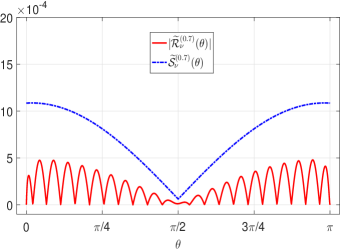
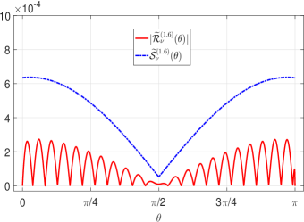
Figure 2.1. Plots of $|\widetilde{\mathcal{R}}_{\nu}^{(\lambda)}(\theta)|$ and $\widetilde{\mathcal{S}}_{\nu}^{(\lambda)}(\theta)$ in Theorem 2.2, where $\theta\in[0,\pi],\lambda=0.7,1.6,2.3,3.1$ and $\nu=20.3$.

In the end of this section, we provide some numerical illustrations of the unform bounds in Theorem 2.2. In Figure 2.1, we plot the graphs of $|\widetilde{\mathcal{R}}_{\nu}^{(\lambda)}(\theta)|$ and $\widetilde{\mathcal{S}}_{\nu}^{(\lambda)}(\theta)$ for $\theta\in[0,\pi]$ and with $\lambda=0.7,1.6,2.3,3.1,$ $\nu=20.3$. Indeed, we observe that in all cases, the curves of the upper bounds are on the top of $|\widetilde{\mathcal{R}}_{\nu}^{(\lambda)}(\theta)|,$ and “sharp” corner of $\widetilde{\mathcal{S}}_{\nu}^{(\lambda)}(\theta)$ at $\theta=\pi/2$ is largely due to the involved $|\cos\theta|.$

3. Proof of the results

3.1. Two lemmas

As the proof of the main result is quite involved, we take several steps and summarise the intermediate results into two lemmas.

3.2. Uniform upper bounds

The bounds stated in the following two theorems are indispensable for the forthcoming error analysis.

Lemma 3.1.

For real $0<\lambda<1$, we have

$$\max_{|x|\leq 1}\big{\{}(1-x^{2})^{\lambda/2}\big{|}{}^{r\!}G_{\nu}^{(\lambda)}(x)\big{|},\;(1-x^{2})^{\lambda/2}\big{|}{}^{l}G_{\nu}^{(\lambda)}(x)\big{|}\big{\}}\leq\widehat{\kappa}_{\nu}^{(\lambda)},\;\;\;\nu\geq 0,$$ (3.1)

where

$$\begin{split}\widehat{\kappa}_{\nu}^{(\lambda)}=\frac{\Gamma(\lambda+1/2)}{\sqrt{\pi}}\bigg{(}\frac{\cos^{2}(\pi\nu/2)\Gamma^{2}(\nu/2+1/2)}{\Gamma^{2}(({\nu}+1)/2+\lambda)}+\frac{4\sin^{2}\big{(}\pi{\nu}/2\big{)}}{\nu^{2}+2\lambda\nu+\lambda}\frac{\Gamma^{2}(\nu/2+1)}{\Gamma^{2}({\nu}/2+\lambda)}\bigg{)}^{\frac{1}{2}}.\end{split}$$ (3.2)

Lemma 3.2.

For real $\lambda\geq 1$, we have

$$\max_{|x|\leq 1}\big{\{}\omega_{\lambda}(x)\big{|}{}^{r\!}G_{\nu}^{(\lambda)}(x)\big{|},\;\omega_{\lambda}(x)\big{|}{}^{l}G_{\nu}^{(\lambda)}(x)\big{|}\big{\}}\leq\frac{\Gamma(\lambda+1/2)}{\sqrt{\pi}}\frac{\Gamma(({\nu}+1)/2)}{\Gamma(({\nu}+1)/2+\lambda)},\;\;\;\nu\geq 0,$$ (3.3)

where $\omega_{\lambda}(x)=(1-x^{2})^{\lambda-1/2}$.

Theorem 3.1.

For real $\lambda>1$, we have the bound: for $x^{2}\leq 1-{\lambda(\lambda-1)}/{(\lambda+\nu)^{2}}$,

$$\max\big{\{}(1-x^{2})^{\lambda/2}\big{|}{}^{r\!}G_{\nu}^{(\lambda)}(x)\big{|},\;(1-x^{2})^{\lambda/2}\big{|}{}^{l}G_{\nu}^{(\lambda)}(x)\big{|}\big{\}}\leq\widehat{\kappa}_{\nu}^{(\lambda)},\;\;\;\nu\geq 0,$$ (3.4)

where

$$\begin{split}\widehat{\kappa}_{\nu}^{(\lambda)}=\frac{\Gamma(\lambda+1/2)}{\sqrt{\pi}}\bigg{(}\frac{\cos^{2}(\pi\nu/2)\Gamma^{2}(\nu/2+1/2)}{\Gamma^{2}(({\nu}+1)/2+\lambda)}+\frac{4\sin^{2}\big{(}\pi{\nu}/2\big{)}}{\nu^{2}+2\lambda\nu+\lambda}\frac{\Gamma^{2}(\nu/2+1)}{\Gamma^{2}({\nu}/2+\lambda)}\bigg{)}^{\frac{1}{2}}.\end{split}$$ (3.5)

Proof.

To be revised in the earlier paper! Thanks to (LABEL:obsvers), it suffices to prove the result for ${}^{r\!}G_{\nu}^{(\lambda)}(x).$

We denote

$$\begin{split}&\widehat{M}(x):=(1-x^{2})^{\lambda/2}{}^{r\!}G_{\nu}^{(\lambda)}(x);\quad\widehat{H}(x):=\widehat{M}^{2}(x)+\frac{1}{\rho(x)}\big{(}\widehat{M}^{\prime}(x)\big{)}^{2},\\ &\rho(x):=\big{(}(\nu+\lambda)^{2}(1-x^{2})-\lambda(\lambda-1)\big{)}(1-x^{2})^{-2}.\end{split}$$ (3.6)

Note that by Proposition LABEL:nonvember, $\widehat{H}(x)$ is continuous on $[-1,1].$

Taking $a=-\nu,b=\nu+2\lambda,c=\lambda+1/2$ and $z=(1\pm x)/2$ in (4.4), we find that $G(x)$ satisfies the Sturm-Liouville problem

$$\begin{split}\big{(}\omega_{\lambda+1}(x)G^{\prime}(x)\big{)}^{\prime}+\nu(\nu+2\lambda)\omega_{\lambda}(x)G(x)=0,\quad x\in(-1,1).\end{split}$$ (3.7)

A direct calculation from (3.7) leads to

$$(1-x^{2})\widehat{M}^{\prime\prime}(x)-x\widehat{M}^{\prime}(x)+(1-x^{2})\rho(x)\widehat{M}(x)=0,\quad x\in(-1,1).$$ (3.8)

Thus, we have

$$\begin{split}\widehat{H}^{\prime}(x)&=\frac{2\lambda(\lambda-1)x}{(\lambda+\nu)^{2}(1-x^{2})^{2}-\lambda(\lambda-1)(1-x^{2})}\big{(}\widehat{M}^{\prime}(x)\big{)}^{2},\quad x\in(-1,1).\end{split}$$ (3.9)

Hence, for $x^{2}\leq 1-{\lambda(\lambda-1)}/{(\lambda+\nu)^{2}},$ $\widehat{H}(x)$ is increasing for $-\sqrt{1-{\lambda(\lambda-1)}/{(\lambda+\nu)^{2}}}\leq x<0,$ and decreasing for $0<x\leq\sqrt{1-{\lambda(\lambda-1)}/{(\lambda+\nu)^{2}}},$ so we have

$$\widehat{M}^{2}(x)\leq\widehat{H}(x)\leq\widehat{H}(0)=\widehat{M}^{2}(0)+{\rho^{-1}(0)}\big{(}\widehat{M}^{\prime}(0)\big{)}^{2},\quad\forall\,x\in[-1,1].$$ (3.10)

By (4.5) and (4.5), we obtain that for $\lambda\geq 0,$

$$\begin{split}M(0)&={}^{r\!}G_{\nu}^{(\lambda)}(0)={}_{2}F_{1}\Big{(}\!\!-\nu,\nu+2\lambda;\lambda+\frac{1}{2};\frac{1}{2}\Big{)}=\frac{\sqrt{\pi}\,\Gamma(\lambda+1/2)}{\Gamma(-{\nu}/2+1/2)\Gamma({\nu}/2+\lambda+1/2)}\\ &=\sin\big{(}\pi({\nu}+1)/2\big{)}\frac{\Gamma(\lambda+1/2)\Gamma({\nu}/2+1/2)}{\sqrt{\pi}\,\Gamma({\nu}/2+\lambda+1/2)}.\end{split}$$ (3.11)

By (3.11), we have

$$\begin{split}\widehat{M}(0)&=\cos\big{(}\pi{\nu}/2\big{)}\frac{\Gamma(\lambda+1/2)\Gamma({\nu}/2+1/2)}{\sqrt{\pi}\,\Gamma({\nu}/2+\lambda+1/2)}.\end{split}$$ (3.12)

Recall the identity (cf. [17, (15.5.1)]):

$$\frac{d}{dx}{}_{2}F_{1}(a,b;c;z)=\frac{ab}{c}{}_{2}F_{1}(a+1,b+1;c+1;z).$$ (3.13)

By (2.1) and (3.13), we obtain

$$\begin{split}\frac{d}{dx}{}^{r\!}G_{\nu}^{(\lambda)}(x)&=\frac{d}{dx}{}_{2}F_{1}\Big{(}\!\!-\nu,\nu+2\lambda;\lambda+\frac{1}{2};\frac{1-x}{2}\Big{)}\\ &=\frac{\nu(\nu+2\lambda)}{2\lambda+1}{}_{2}F_{1}\Big{(}\!\!-\nu+1,\nu+2\lambda+1;\lambda+\frac{3}{2};\frac{1-x}{2}\Big{)}.\end{split}$$ (3.14)

If $\nu>1/2$, using (3.14), we have

$$\begin{split}\frac{d}{dx}{}^{r\!}G_{\nu}^{(\lambda)}(x)=\frac{\nu(\nu+2\lambda)}{2\lambda+1}{}^{r\!}G_{\nu-1}^{(\lambda+1)}(x).\end{split}$$ (3.15)

Thanks to

$$\widehat{M}^{\prime}(x)=-\lambda x(1-x^{2})^{\lambda/2-1}\,{}^{r\!}G_{\nu}^{(\lambda)}(x)+(1-x^{2})^{\lambda/2}\frac{d}{dx}{}^{r\!}G_{\nu}^{(\lambda)}(x),$$

with (4.5), (4.5) and (3.14), we obtain

$$\begin{split}\{\rho^{-1/2}(x)\widehat{M}^{\prime}(x)\}|_{x=0}&=\frac{2\sin(\pi\nu/2)}{\sqrt{\pi}}\frac{\Gamma(\nu/2+1)\,\Gamma(\lambda+1/2)}{\sqrt{\nu^{2}+2\lambda\nu+\lambda}\,\,\Gamma(\lambda+\nu/2)}.\end{split}$$ (3.16)

From (3.10), (3.12) and (3.16), we derive (3.4). ∎

Lemma 3.3.

For real $\lambda>0,$ $\theta\in(0,\pi)$ and $t>0,$ define

$$\begin{split}&g(\theta,t):=\frac{\cos(\theta-{\rm i}t)-\cos\theta}{t}=\frac{\cos\theta\,(\cosh t-1)+{\rm i}\sin\theta\,\sinh t}{t},\\ &f^{(\lambda)}(\theta,t):=\frac{g^{\lambda-1}(\theta,t)-g^{\lambda-1}(\theta,0)}{t},\quad g(\theta,0):=\lim_{t\to 0^{+}}g(\theta,t)={\rm i}\sin\theta.\end{split}$$ (3.17)

Then we have for $\theta\in(0,\pi)$ and $t>0,$

• for $0<\lambda\leq 2,$

  $$|f^{(\lambda)}(\theta,t)|\leq|\lambda-1|\,(\sin\theta)^{\lambda-1}\,\Big{(}|\cot\theta|+\frac{2t}{3}\Big{)}e^{t};$$ (3.18)

• for $\lambda>2,$

  $$|f^{(\lambda)}(\theta,t)|\leq 2^{\lambda/2}\,(\lambda-1)\,(\sin\theta)^{\lambda-1}\,\Big{(}|\cot\theta|+\frac{2t}{3}\Big{)}\Big{(}1+\frac{|\cot\theta|^{\lambda-2}}{2^{\lambda-2}}\,t^{\lambda-2}e^{(\lambda-2)t}\Big{)}e^{(\lambda-1)t}.$$ (3.19)

To avoid distracting from proving the main result, we put this a bit lengthy proof but only involving fundamental calculus in Appendix E.

A critical step is to show that the integral in (2.9) satisfies the following identity.

Lemma 3.4.

For real $\nu,\lambda\geq 0,$ and $\theta\in(0,\pi),$ we have

$$\int^{\theta}_{0}\frac{\cos((\nu+\lambda)\phi)}{(\cos\phi-\cos\theta)^{1-\lambda}}\,d\phi=\frac{\Gamma(\lambda)}{(\nu+\lambda)^{\lambda}}\,\frac{\cos((\nu+\lambda)\theta-\lambda\pi/2)}{(\sin\theta)^{1-\lambda}}+\breve{\mathcal{R}}_{\nu}^{(\lambda)}(\theta),$$ (3.20)

where

$$\begin{split}&\breve{\mathcal{R}}_{\nu}^{(\lambda)}(\theta):=\int^{\infty}_{0}\Re\big{\{}{\rm i}\,e^{-{\rm i}(\nu+\lambda)\theta}f^{(\lambda)}(\theta,t)\big{\}}t^{\lambda}e^{-(\nu+\lambda)t}dt,\end{split}$$ (3.21)

and $f^{(\lambda)}(\theta,t)$ is defined in (3.17).

Proof.

It is evident that by the parity, we have

$$\int^{\theta}_{0}\frac{\cos((\nu+\lambda)\phi)}{(\cos\phi-\cos\theta)^{1-\lambda}}\,d\phi=\frac{1}{2}\int^{\theta}_{-\theta}F_{\nu}^{(\lambda)}(\theta,\phi)\,d\phi\,,$$ (3.22)

where we denote

$$F_{\nu}^{(\lambda)}(\theta,\phi):=\frac{e^{{\rm i}(\nu+\lambda)\phi}}{(\cos\phi-\cos\theta)^{1-\lambda}}\,.$$ (3.23)

We consider the cases with $\lambda\geq 1$ and $0<\lambda<1,$ separately. (i) Proof of (3.20) with $\lambda\geq 1$.  From the Cauchy-Goursat theorem, we infer that for any fixed $\theta\in(0,\pi)$ and real $\nu>0,$ the contour integration of $F_{\nu}^{(\lambda)}(\theta,\cdot)$ (with an extension to the complex plane) along the rectangular contour in Figure 3.1 (left), is zero. Thus, we have

$$\begin{split}\int^{\theta}_{-\theta}F_{\nu}^{(\lambda)}(\theta,\phi)\,d\phi&=\int^{-\theta+{\rm i}R}_{-\theta}F_{\nu}^{(\lambda)}(\theta,\phi)\,d\phi-\int^{\theta+{\rm i}R}_{\theta}F_{\nu}^{(\lambda)}(\theta,\phi)\,d\phi+\int^{\theta+{\rm i}R}_{-\theta+{\rm i}R}F_{\nu}^{(\lambda)}(\theta,\phi)\,d\phi\\ &={\rm i}\int_{0}^{R}\big{\{}F_{\nu}^{(\lambda)}(\theta,-\theta+{\rm i}t)-F_{\nu}^{(\lambda)}(\theta,\theta+{\rm i}t)\big{\}}dt+\int^{\theta}_{-\theta}F_{\nu}^{(\lambda)}(\theta,t+{\rm i}R)\,dt,\end{split}$$ (3.24)

where we made the change of variables for three integrals: $\phi=-\theta+{\rm i}t,\theta+{\rm i}t,t+{\rm i}R,$ respectively.

Figure 3.1. Contour integral for (3.24). Left: for $\lambda\geq 1$; Right: for $0<\lambda<1$.

For $\lambda\geq 1$ and $R>0,$ we have

$$\begin{split}|F_{\nu}^{(\lambda)}(\theta,t+{\rm i}R)|&=\frac{|e^{{\rm i}(\nu+\lambda)t-(\nu+\lambda)R}|}{|\cos(t+{\rm i}R)-\cos\theta|^{1-\lambda}}\\ &=e^{-(\nu+\lambda)R}\big{(}(\cos t\cosh R-\cos\theta)^{2}+\sin^{2}t\sinh^{2}R\big{)}^{(\lambda-1)/2}\\ &\leq e^{-(\nu+\lambda)R}\big{(}(\cosh R+1)^{2}+\sinh^{2}R\big{)}^{(\lambda-1)/2}\\ &=2^{(1-\lambda)/2}e^{-(\nu+1)R}\big{(}1+2e^{-R}+2e^{-2R}+2e^{-3R}+e^{-4R}\big{)}^{(\lambda-1)/2}\\ &<2^{\lambda-1}e^{-(\nu+1)R}.\end{split}$$ (3.25)

Thus, we have

$$\lim_{R\to\infty}\int^{\theta+{\rm i}R}_{-\theta+{\rm i}R}F_{\nu}^{(\lambda)}(\theta,\phi)\,d\phi=\lim_{R\to\infty}\int^{\theta}_{-\theta}F_{\nu}^{(\lambda)}(\theta,t+{\rm i}R)\,dt=0.$$ (3.26)

Recall the notation in (3.17): $tg(\theta,t)=\cos(\theta-{\rm i}t)-\cos\theta.$ In view of (3.17), we can write $g^{\lambda-1}(\theta,t)=g^{\lambda-1}(\theta,0)+tf^{(\lambda)}(\theta,t).$ Thus, by a direct calculation, we obtain

$$\begin{split}{\rm i}F_{\nu}^{(\lambda)}(\theta,-\theta+{\rm i}t)&-{\rm i}F_{\nu}^{(\lambda)}(\theta,\theta+{\rm i}t)\\ &=\big{\{}{\rm i}\,g^{\lambda-1}(\theta,t)e^{-{\rm i}(\nu+\lambda)\theta}+\big{(}{\rm i}\,g^{\lambda-1}(\theta,t)e^{-{\rm i}(\nu+\lambda)\theta}\big{)}^{*}\big{\}}t^{\lambda-1}e^{-(\nu+\lambda)t}\\ &=2\,\Re\big{\{}{\rm i}\,g^{\lambda-1}(\theta,t)e^{-{\rm i}(\nu+\lambda)\theta}\big{\}}t^{\lambda-1}e^{-(\nu+\lambda)t}\\ &=2\,\Re\big{\{}{\rm i}\,g^{\lambda-1}(\theta,0)e^{-{\rm i}(\nu+\lambda)\theta}\big{\}}t^{\lambda-1}e^{-(\nu+\lambda)t}\\ &\quad+2\,\Re\big{\{}{\rm i}\,f^{(\lambda)}(\theta,t)e^{-{\rm i}(\nu+\lambda)\theta}\big{\}}t^{\lambda}e^{-(\nu+\lambda)t}.\end{split}$$ (3.27)

Since ${\rm i}=e^{{\rm i}\pi/2}$ and $g(\theta,0)=({\rm i}\sin\theta)^{\lambda-1}$, we have

$$\begin{split}\Re\big{\{}{\rm i}\,g^{\lambda-1}(\theta,0)e^{-{\rm i}(\nu+\lambda)\theta}\big{\}}&=\Re\big{\{}{\rm i}\,({\rm i}\sin\theta)^{\lambda-1}\,e^{-{\rm i}(\nu+\lambda)\theta}\big{\}}=(\sin\theta)^{\lambda-1}\,\Re\big{\{}e^{-{\rm i}((\nu+\lambda)\theta-\lambda\pi/2)}\big{\}}\\ &=(\sin\theta)^{\lambda-1}\cos((\nu+\lambda)\theta-\lambda\pi/2).\end{split}$$ (3.28)

Using the definition of the Gamma function, we find that for any $a>0,z>-1,$

$$\begin{split}\int^{\infty}_{0}t^{z}e^{-at}dt=\frac{\Gamma(z+1)}{a^{z+1}},\;\;\;{\rm as}\;\;\;\Gamma(z+1)=\int^{\infty}_{0}e^{-t}t^{z}dt.\end{split}$$ (3.29)

As a direct consequence of (3.28)-(3.29), we have

$$2\,\int_{0}^{\infty}\Re\big{\{}{\rm i}\,g^{\lambda-1}(\theta,0)e^{-{\rm i}(\nu+\lambda)\theta}\big{\}}t^{\lambda-1}e^{-(\nu+\lambda)t}dt=\frac{2\,\Gamma(\lambda)}{(\nu+\lambda)^{\lambda}}\,\frac{\cos((\nu+\lambda)\theta-\lambda\pi/2)}{(\sin\theta)^{1-\lambda}}.$$ (3.30)

Letting $R\to\infty$ in (3.24), we obtain (3.20)-(3.21) from (3.22), (3.26)-(3.27) and (3.30) directly.

(ii) Proof of (3.20) with $0<\lambda<1$.  In this case, we integrate along a similar contour but exclude singular points $\phi=\pm\theta,$ as depicted in Figure 3.1 (right), where $0<\epsilon<\theta.$ Like (3.24), we have

$$\begin{split}\int^{\theta-\epsilon}_{-\theta+\epsilon}F_{\nu}^{(\lambda)}(\theta,&\phi)\,d\phi=I_{1}(\epsilon,R)+I_{2}(R)+I_{3}(\epsilon)+I_{4}(\epsilon),\end{split}$$ (3.31)

where

$$\begin{split}&I_{1}(\epsilon,R):=\int^{-\theta+{\rm i}R}_{-\theta+{\rm i}\epsilon}F_{\nu}^{(\lambda)}(\theta,\phi)\,d\phi-\int^{\theta+{\rm i}R}_{\theta+{\rm i}\epsilon}F_{\nu}^{(\lambda)}(\theta,\phi)\,d\phi,\\ &I_{2}(R):=\int^{\theta+{\rm i}R}_{-\theta+{\rm i}R}F_{\nu}^{(\lambda)}(\theta,\phi)\,d\phi,\\ &I_{3}(\epsilon):=\int_{-\theta+\epsilon}^{-\theta+\epsilon+{\rm i}\epsilon}F_{\nu}^{(\lambda)}(\theta,\phi)\,d\phi-\int_{\theta-\epsilon}^{\theta-\epsilon+{\rm i}\epsilon}F_{\nu}^{(\lambda)}(\theta,\phi)\,d\phi\\ &I_{4}(\epsilon):=-\int_{-\theta+{\rm i}\epsilon}^{-\theta+\epsilon+{\rm i}\epsilon}F_{\nu}^{(\lambda)}(\theta,\phi)\,d\phi-\int_{\theta-\epsilon+{\rm i}\epsilon}^{\theta+{\rm i}\epsilon}F_{\nu}^{(\lambda)}(\theta,\phi)\,d\phi.\end{split}$$ (3.32)

Using a change of variable: $\phi=\pm\theta+{\rm i}t,$ and noting that the derivation in (3.27)-(3.28) is valid for $0<\lambda<1,$ we have

$$\begin{split}I_{1}(\epsilon,R)&={\rm i}\int_{\epsilon}^{R}\big{\{}F_{\nu}^{(\lambda)}(\theta,-\theta+{\rm i}t)-F_{\nu}^{(\lambda)}(\theta,\theta+{\rm i}t)\big{\}}dt\\ &=2\frac{\cos((\nu+\lambda)\theta-\lambda\pi/2)}{(\sin\theta)^{1-\lambda}}\int_{\epsilon}^{R}t^{\lambda-1}e^{-(\nu+\lambda)t}dt\\ &\quad+2\,\int_{\epsilon}^{R}\Re\big{\{}{\rm i}\,f^{(\lambda)}(\theta,t)e^{-{\rm i}(\nu+\lambda)\theta}\big{\}}t^{\lambda}e^{-(\nu+\lambda)t}dt.\end{split}$$ (3.33)

From (3.18) and (3.29) -(3.30), we infer that

$$\begin{split}\lim_{\epsilon\to 0;R\to\infty}I_{1}(\epsilon,R)&=\frac{2\,\Gamma(\lambda)}{(\nu+\lambda)^{\lambda}}\,\frac{\cos((\nu+\lambda)\theta-\lambda\pi/2)}{(\sin\theta)^{1-\lambda}}\\ &\quad+2\,\int_{0}^{\infty}\Re\big{\{}{\rm i}\,f^{(\lambda)}(\theta,t)e^{-{\rm i}(\nu+\lambda)\theta}\big{\}}t^{\lambda}e^{-(\nu+\lambda)t}dt.\end{split}$$ (3.34)

Therefore, it suffices to show

$$\begin{split}\lim_{R\to\infty}I_{2}(R)=0,\quad\lim_{\epsilon\to 0}I_{3}(\epsilon)=\lim_{\epsilon\to 0}I_{4}(\epsilon)=0.\end{split}$$ (3.35)

By (3.24), we have

$$I_{2}(R)=\int^{\theta}_{-\theta}F_{\nu}^{(\lambda)}(\theta,t+{\rm i}R)\,dt,$$ (3.36)

and

$$\begin{split}|F_{\nu}^{(\lambda)}(\theta,t+{\rm i}R)|&=\frac{|e^{{\rm i}(\nu+\lambda)t-(\nu+\lambda)R}|}{|\cos(t+{\rm i}R)-\cos\theta|^{1-\lambda}}\\ &=e^{-(\nu+\lambda)R}\big{(}(\cos t\cosh R-\cos\theta)^{2}+\sin^{2}t\sinh^{2}R\big{)}^{(\lambda-1)/2}\\ &\leq e^{-(\nu+\lambda)R}(\sinh R)^{\lambda-1}|\sin t|^{\lambda-1}.\end{split}$$ (3.37)

Thus, for $0<\lambda<1$ and $\theta\in(0,\pi),$

$$|I_{2}(R)|\leq\frac{2e^{-(\nu+\lambda)R}}{(\sinh R)^{1-\lambda}}\int_{0}^{\theta}\frac{1}{(\sin t)^{1-\lambda}}dt\to 0,\;\;\;{\rm as}\;\;R\to\infty.$$ (3.38)

Next, using a change of variable: $\theta=-\theta+\epsilon+{\rm i}t,\theta-\epsilon+{\rm i}t,$ respectively, for two integrals, we obtain from a direct calculation that

$$\begin{split}I_{3}(\epsilon)&={\rm i}\int_{0}^{\epsilon}\big{\{}F_{\nu}^{(\lambda)}(\theta,-\theta+\epsilon+{\rm i}t)-F_{\nu}^{(\lambda)}(\theta,\theta-\epsilon+{\rm i}t)\big{\}}dt\\ &=2\int_{0}^{\epsilon}\Re\Big{\{}\frac{{\rm i}e^{-{\rm i}(\nu+\lambda)(\theta-\epsilon)}}{(\cos(\theta-\epsilon-{\rm i}t)-\cos\theta)^{1-\lambda}}\Big{\}}e^{-(\nu+\lambda)t}dt.\end{split}$$ (3.39)

Note that we have

$$\begin{split}|\cos(\theta-\epsilon-{\rm i}t)-\cos\theta|&=((\cos(\theta-\epsilon)\cosh t-\cos\theta)^{2}+\sin^{2}(\theta-\epsilon)\sinh^{2}t)^{1/2}\\ &\geq|\sin(\theta-\epsilon)||\sinh t|\geq|\sin(\theta-\epsilon)||\sin t|,\end{split}$$ (3.40)

where we used the inequality: $|\sin t|\leq\sinh t$ for $t>0$ (cf. [17, (4.18.9)]). Therefore, for $0<\lambda<1,$ we have

$$|I_{3}(\epsilon)|\leq\frac{2}{(\sin(\theta-\epsilon))^{1-\lambda}}\int_{0}^{\epsilon}{(\sin t)^{\lambda-1}}dt\to 0,\;\;\;{\rm as}\;\;\epsilon\to 0.$$ (3.41)

Similarly, with a change of variable: $\theta=-\theta+{\rm i}\epsilon+t,\theta+{\rm i}\epsilon-t,$ respectively, for two integrals,

$$\begin{split}I_{4}(\epsilon)&=-\int_{0}^{\epsilon}\big{\{}F_{\nu}^{(\lambda)}(\theta,-\theta+{\rm i}\epsilon+t)+F_{\nu}^{(\lambda)}(\theta,\theta+{\rm i}\epsilon-t)\big{\}}dt\\ &=-2e^{-\epsilon(\nu+\lambda)}\int_{0}^{\epsilon}\Re\Big{\{}\frac{e^{{\rm i}(\nu+\lambda)(t-\theta)}}{(\cos(t-\theta+{\rm i}\epsilon)-\cos\theta)^{1-\lambda}}\Big{\}}dt.\end{split}$$ (3.42)

It is evident that

$$\begin{split}|\cos(t-\theta+{\rm i}\epsilon)-\cos\theta|&=\big{(}(\cos(t-\theta)\cosh\epsilon-\cos\theta)^{2}+\sin^{2}(t-\theta)\sinh^{2}\epsilon\big{)}^{1/2}\\ &\geq\sin(\theta-t)\sinh\epsilon,\end{split}$$ (3.43)

where as $0<\theta<\pi$ and $0<t<\epsilon<\theta$, we have

$$0<\theta-\epsilon<\theta-t<\theta<\pi.$$

By the fundamental inequalities,

$$\frac{2}{\pi}z\leq\sin z\leq z,\quad z\in(0,\pi/2),$$ (3.44)

we obtain

$$\frac{1}{\sin z}=\frac{1}{\sin(\pi-z)}\leq\frac{\pi}{2}\max\Big{\{}\frac{1}{z},\frac{1}{\pi-z}\Big{\}},\quad z\in(0,\pi).$$ (3.45)

This implies

$$\sin(\theta-t)\geq\frac{2}{\pi}\min\big{\{}\theta-t,\pi-\theta+t\big{\}}>\frac{2}{\pi}\min\big{\{}\theta-\epsilon,\pi-\theta\big{\}}.$$ (3.46)

From (3.42) and (3.46), we obtain

$$\begin{split}|I_{4}(\epsilon)|&\leq 2e^{-\epsilon(\nu+\lambda)}\int_{0}^{\epsilon}|\cos(t-\theta+{\rm i}\epsilon)-\cos\theta|^{\lambda-1}dt\\ &\leq\frac{2^{\lambda}}{\pi^{\lambda-1}}\,\frac{\epsilon}{(\sinh\epsilon)^{1-\lambda}}\max\big{\{}(\theta-\epsilon)^{\lambda-1},(\pi-\theta)^{\lambda-1}\big{\}}\to 0,\;\;{\rm as}\;\;\epsilon\to 0.\end{split}$$ (3.47)

Thus, letting $\epsilon\to 0$ and $R\to\infty$ in (3.31), we obtain (3.20)-(3.21) with $0<\lambda<1$ from (3.22), (3.34), (3.38), (3.41) and (3.47). ∎

3.3. Proof of Theorem 2.1

With the bounds and identity in Lemmas 3.3-3.4, we are ready to show the main result.

From (2.9) and Lemma 3.4, we derive

$$\begin{split}{\mathcal{R}}_{\nu}^{(\lambda)}(\theta)&=\frac{2^{\lambda}\,\Gamma(\lambda+1/2)}{\sqrt{\pi}\,\Gamma(\lambda)}(\sin\theta)^{1-\lambda}\,\breve{\mathcal{R}}_{\nu}^{(\lambda)}(\theta)\\ &=\frac{2^{\lambda}\,\Gamma(\lambda+1/2)}{\sqrt{\pi}\,\Gamma(\lambda)}(\sin\theta)^{1-\lambda}\int^{\infty}_{0}\Re\big{\{}{\rm i}\,e^{-{\rm i}(\nu+\lambda)\theta}f^{(\lambda)}(\theta,t)\big{\}}t^{\lambda}e^{-(\nu+\lambda)t}dt.\end{split}$$ (3.48)

We now estimate $\breve{\mathcal{R}}_{\nu}^{(\lambda)}(\theta)$ in (3.20)-(3.21) by using Lemma 3.3.

(i) For $0<\lambda\leq 2$ and $\nu+\lambda>1,$ we obtain from (3.18) and (3.29) that

$$\begin{split}|\breve{\mathcal{R}}_{\nu}^{(\lambda)}(\theta)|&\leq\int^{\infty}_{0}|f^{(\lambda)}(\theta,t)|\,t^{\lambda}e^{-(\nu+\lambda)t}dt\\ &\leq|\lambda-1|\,(\sin\theta)^{\lambda-1}\,\int^{\infty}_{0}\Big{(}|\cot\theta|+\frac{2t}{3}\Big{)}\,t^{\lambda}e^{-(\nu+\lambda-1)t}dt\\ &=\frac{|\lambda-1|\,\Gamma(\lambda+1)}{(\nu+\lambda-1)^{\lambda+1}}(\sin\theta)^{\lambda-1}\big{(}|\cot\theta|+\frac{2}{3}\frac{\lambda+1}{\nu+\lambda-1}\Big{)}.\end{split}$$ (3.49)

(ii) For $\lambda>2$ and $\nu>\lambda-3,$ we derive from (3.19) and (3.29) that

$$\begin{split}|\breve{\mathcal{R}}_{\nu}^{(\lambda)}&(\theta)|\leq\int^{\infty}_{0}|f^{(\lambda)}(\theta,t)|\,t^{\lambda}e^{-(\nu+\lambda)t}dt\\ &\leq 2^{\lambda/2}(\lambda-1)(\sin\theta)^{\lambda-1}\int^{\infty}_{0}\Big{(}|\cot\theta|+\frac{2t}{3}\Big{)}\Big{(}1+\frac{|\cot\theta|^{\lambda-2}}{2^{\lambda-2}}\,t^{\lambda-2}e^{(\lambda-2)t}\Big{)}t^{\lambda}e^{-(\nu+1)t}dt\\ &=\frac{2^{\lambda/2}(\lambda-1)\,\Gamma(\lambda+1)}{(\nu+1)^{\lambda+1}}\,(\sin\theta)^{\lambda-1}\Big{\{}|\cot\theta|+\frac{2}{3}\frac{\lambda+1}{\nu+1}\\ &\quad+\frac{2^{2-\lambda}\Gamma(2\lambda-1)}{\Gamma(\lambda+1)}\frac{(\nu+1)^{\lambda+1}}{(\nu-\lambda+3)^{2\lambda-1}}|\cot\theta|^{\lambda-2}\Big{(}|\cot\theta|+\frac{2}{3}\frac{2\lambda-1}{\nu-\lambda+3}\Big{)}\Big{\}}.\end{split}$$ (3.50)

Thanks to (3.48), we can derive the bounds in (2.14)-(2.15) from this relation and (3.49)-(3.50), respectively. This completes the proof of Theorem 2.1.

3.4. Proof of Corollary 2.1

We prove two cases separately.

(i) We obtain from (2.14) that

$$\begin{split}{\nu^{\lambda+1}\sin\theta}\,{|{\mathcal{R}}_{\nu}^{(\lambda)}(\theta)|}&\leq\frac{\lambda|\lambda-1|2^{\lambda}\Gamma(\lambda+1/2)}{\sqrt{\pi}}\Big{(}|\cos\theta|+\frac{2}{3}\frac{(\lambda+1)\sin\theta}{\nu+\lambda-1}\Big{)}\Big{(}1+\frac{1-\lambda}{\nu+\lambda-1}\Big{)}^{\lambda+1}\\ &\leq\frac{\lambda|\lambda-1|2^{\lambda}\Gamma(\lambda+1/2)}{\sqrt{\pi}}\Big{(}1+\frac{2}{3}\frac{\lambda+1}{\nu+\lambda-1}\Big{)}\Big{(}1+\frac{1-\lambda}{\nu+\lambda-1}\Big{)}^{\lambda+1}.\end{split}$$ (3.51)

Using the basic inequality: $\ln(1+z)\leq z$ for $z>-1,$ we find

$$\begin{split}\Big{(}1+\frac{1-\lambda}{\nu+\lambda-1}\Big{)}^{\lambda+1}&={\rm exp}\Big{(}{(\lambda+1)\ln\Big{(}1+\frac{1-\lambda}{\nu+\lambda-1}\Big{)}}\Big{)}\leq{\rm exp}\Big{(}\frac{1-\lambda^{2}}{\nu+\lambda-1}\Big{)}.\end{split}$$ (3.52)

Thus, we obtain $B_{\nu}^{(\lambda)}$ immediately from the above for this case.

(ii) For $\lambda>2,$ $\nu-\lambda+3\geq 0$ and $\theta\in[c\nu^{-1},\pi-c\nu^{-1}]$, we obtain from (2.15) that

$$\begin{split}&{\nu^{\lambda+1}\sin\theta}\,{|{\mathcal{R}}_{\nu}^{(\lambda)}(\theta)|}\leq\frac{\lambda(\lambda-1)2^{3/2\lambda}\Gamma(\lambda+1/2)}{\sqrt{\pi}}\frac{\nu^{\lambda+1}}{(\nu+1)^{\lambda+1}}\Big{\{}|\cos\theta|+\frac{2}{3}\frac{\lambda+1}{\nu+1}\sin\theta\\ &\;\;\;\;+\frac{2^{2-\lambda}\Gamma(2\lambda-1)}{\Gamma(\lambda+1)}\frac{(\nu+1)^{\lambda+1}}{(\nu-\lambda+3)^{2\lambda-1}}|\cot\theta|^{\lambda-2}\Big{(}|\cos\theta|+\frac{2}{3}\frac{2\lambda-1}{\nu-\lambda+3}\sin\theta\Big{)}\Big{\}}.\end{split}$$ (3.53)

It is evident that

$$\begin{split}|\cos\theta|+\frac{2}{3}\frac{\lambda+1}{\nu+1}\sin\theta\leq\frac{3\nu+2\lambda+5}{3(\nu+1)},\;\;|\cos\theta|+\frac{2}{3}\frac{2\lambda-1}{\nu-\lambda+3}\sin\theta\leq\frac{3\nu+\lambda+7}{3(\nu-\lambda+3)}.\end{split}$$ (3.54)

We write

$$\frac{(\nu+1)^{\lambda+1}|\cot\theta|^{\lambda-2}}{(\nu-\lambda+3)^{2\lambda-1}}=\Big{(}\frac{\nu+1}{\nu-\lambda+3}\Big{)}^{\lambda+1}\,\Big{(}\frac{\nu}{\nu-\lambda+3}\Big{)}^{\lambda-2}\,\Big{(}\frac{|\cot\theta|}{\nu}\Big{)}^{\lambda-2}.$$ (3.55)

Using the inequality: $\ln(1+z)\leq z$ for $z>-1$ again, we derive

$$\begin{split}\Big{(}\frac{\nu+1}{\nu-\lambda+3}\Big{)}^{\lambda+1}={\rm exp}\Big{(}{(\lambda+1)\ln\Big{(}1+\frac{\lambda-2}{\nu-\lambda+3}\Big{)}}\Big{)}\leq{\rm exp}\Big{(}\frac{(\lambda-2)(\lambda+1)}{\nu-\lambda+3}\Big{)},\end{split}$$ (3.56)

and

$$\begin{split}\Big{(}\frac{\nu}{\nu-\lambda+3}\Big{)}^{\lambda-2}={\rm exp}\Big{(}{(\lambda-2)\ln\Big{(}1+\frac{\lambda-3}{\nu-\lambda+3}\Big{)}}\Big{)}\leq{\rm exp}\Big{(}\frac{(\lambda-3)(\lambda+1)}{\nu-\lambda+3}\Big{)}.\end{split}$$ (3.57)

By (3.45), we have

$$\begin{split}\frac{1}{\nu\sin\theta}\leq\frac{\pi}{2}\max\Big{\{}\frac{1}{\nu\theta},\frac{1}{\nu(\pi-\theta)}\Big{\}}\leq\frac{c\pi}{2},\end{split}$$

which implies

$$\begin{split}\Big{(}\frac{|\cot\theta|}{\nu}\Big{)}^{\lambda-2}=|\cos\theta|^{\lambda-2}\Big{(}\frac{1}{\nu\sin\theta}\Big{)}^{\lambda-2}\leq\Big{(}\frac{c\pi}{2}\Big{)}^{\lambda-2}.\end{split}$$ (3.58)

We therefore derive from the above $B_{\nu}^{(\lambda)}$ in the second case.

3.5. Proof of Theorem 2.2

For $\theta\in(0,\pi),$ we can derive the bounds (2.22)-(2.23) from (2.13) by multiplying $\sin\theta$ and $(\sin\theta)^{\lambda-1},$ respectively, for two cases.

In order to derive the upper bounds uniform for both $\nu$ and $\theta,$ it is necessary study the behaviors of ${}^{r\!}G_{\nu}^{(\lambda)}(x)$ at $x=\pm 1$ (i.e., $\theta=0,\pi$). It is evident that by (2.1), ${}^{r\!}G_{\nu}^{(\lambda)}(1)=1$ for all $\lambda>-1/2$ and $\nu\geq 0.$ We now examine the behavior of right GGF-Fs at $x=-1.$ It is clear that if $\nu=n\in{\mathbb{N}}_{0},$ we have ${}^{r\!}G_{n}^{(\lambda)}(-1)=(-1)^{n}\,{}^{r\!}G_{n}^{(\lambda)}(1)=(-1)^{n}.$ We now consider the case with $\nu\notin{\mathbb{N}}_{0}$. Note that for $-1/2<\lambda<1/2$ (cf. [13, Prop. 2.3]):

$${}^{r\!}G_{\nu}^{(\lambda)}(-1)=\frac{\cos((\nu+\lambda)\pi)}{\cos(\lambda\pi)},$$ (3.59)

so ${}^{r\!}G_{\nu}^{(\lambda)}(x)$ is continuous on $[-1,1].$ However, for $\lambda\geq 1/2$ and $\nu\not\in{\mathbb{N}}_{0}$, ${}^{r\!}G_{\nu}^{(\lambda)}(x)$ is singular at $x=-1.$ Indeed, according to [13, Prop. 2.3], we have

$$\lim_{x\to-1^{+}}\frac{{}^{r\!}G_{\nu}^{(1/2)}(x)}{\ln(1+x)}=\frac{\sin(\nu\pi)}{\pi}\,,\quad\nu\not\in{\mathbb{N}}_{0}\,;$$ (3.60)

and for $\lambda>1/2$ and $\nu\not\in{\mathbb{N}}_{0},$ we have

$$\lim_{x\to-1^{+}}\Big{(}\frac{1+x}{2}\Big{)}^{\lambda-1/2}\,{}^{r\!}G_{\nu}^{(\lambda)}(x)=-\frac{\sin(\nu\pi)}{\pi}\frac{\Gamma(\lambda-1/2)\Gamma(\lambda+1/2)\Gamma(\nu+1)}{\Gamma(\nu+2\lambda)}:={\mathcal{Q}}_{\nu}^{(\lambda)}.$$ (3.61)

Note that (3.61) also holds for $\nu=n\in{\mathbb{N}}_{0},$ as ${\mathcal{Q}}_{n}^{(\lambda)}=0.$

We now consider the case with $\theta=0$. As ${}^{r\!}G_{\nu}^{(\lambda)}(1)=1$, taking the limit $\theta\to 0,$ and find readily that the above bounds hold (note: ${\widetilde{\mathcal{R}}^{(\lambda)}_{\nu}}(0)=0$, but ${\widetilde{\mathcal{S}}^{(\lambda)}_{\nu}}(\theta)>0$ in (2.22)-(2.23)).

It remains to consider $\theta\to\pi^{-},$ i.e., $x\to-1^{+}.$ Apparently, we have $\sin\theta=\sqrt{1-x^{2}}.$ As a direct consequence of (3.59)-(3.60), we have that for $0<\lambda\leq 1/2,$

$$\begin{split}\lim_{\theta\to\pi^{-}}\widetilde{\mathcal{R}}_{\nu}^{(\lambda)}(\theta)&=\lim_{\theta\to\pi^{-}}\big{\{}(\sin\theta)^{\lambda+1}\,{}^{r\!}G_{\nu}^{(\lambda)}(\cos\theta)\big{\}}=\lim_{x\to-1^{+}}(1-x^{2})^{(\lambda+1)/2}\,{}^{r\!}G_{\nu}^{(\lambda)}(x)=0.\end{split}$$ (3.62)

Similarly, by (3.61), we have that for $1/2<\lambda<2,$

$$\begin{split}\lim_{\theta\to\pi^{-}}\widetilde{\mathcal{R}}_{\nu}^{(\lambda)}(\theta)&=\lim_{x\to-1^{+}}\big{\{}(1-x^{2})^{1-\lambda/2}(1-x^{2})^{\lambda-1/2}\,{}^{r\!}G_{\nu}^{(\lambda)}(x)\big{\}}=0.\end{split}$$ (3.63)

For $\lambda\geq 2,$ we find from (3.61) that

$$\begin{split}\lim_{\theta\to\pi^{-}}\widetilde{\mathcal{R}}_{\nu}^{(\lambda)}(\theta)&=\lim_{\theta\to\pi^{-}}\big{\{}(\sin\theta)^{2\lambda-1}\,{}^{r\!}G_{\nu}^{(\lambda)}(\cos\theta)\big{\}}=\lim_{x\to-1^{+}}(1-x^{2})^{\lambda-1/2}\,{}^{r\!}G_{\nu}^{(\lambda)}(x)\\ &=2^{2\lambda-1}\,{\mathcal{Q}}_{\nu}^{(\lambda)}.\end{split}$$ (3.64)

(i) For $0<\lambda\leq 2,\,\nu+\lambda>1$ and $\nu>0,$ we find from (2.14) that

$$\lim_{\theta\to\pi^{-}}{\widetilde{\mathcal{S}}^{(\lambda)}_{\nu}}(\theta)=\frac{\lambda|\lambda-1|2^{\lambda}\Gamma(\lambda+1/2)}{\sqrt{\pi}(\nu+\lambda-1)^{\lambda+1}}.$$ (3.65)

Thus, in this case, it is evident that by (3.62)-(3.63) and (3.65), (2.22) holds for $0<\lambda<2$. For $\lambda=2,$ we obtain from (3.64)-(3.65) that

$$\begin{split}\lim_{\theta\to\pi^{-}}\widetilde{\mathcal{R}}_{\nu}^{(2)}(\theta)=2^{3}\,{\mathcal{Q}}_{\nu}^{(2)}=-\frac{3\sin(\nu\pi)}{(\nu+1)(\nu+2)(\nu+3)},\quad\lim_{\theta\to\pi^{-}}{\widetilde{\mathcal{S}}^{(2)}_{\nu}}(\theta)=\frac{6}{(\nu+1)^{3}}.\end{split}$$

Hence, (2.22) holds for $\lambda=2.$

(ii) For $\lambda>2,\,\nu>\lambda-3$ and $\nu>0,$ we obtain from (2.15) that

$$\lim_{\theta\to\pi^{-}}{\widetilde{\mathcal{S}}^{(\lambda)}_{\nu}}(\theta)=\frac{2^{2+\lambda/2}\Gamma(\lambda+1/2)\Gamma(2\lambda-1)}{\sqrt{\pi}(\nu-\lambda+3)^{2\lambda-1}\Gamma(\lambda-1)}=\frac{\lambda\,2^{5\lambda/2}\Gamma(\lambda-1/2)\Gamma(\lambda+1/2)}{\pi(\nu-\lambda+3)^{2\lambda-1}},$$ (3.66)

where we used the identity (cf. [1, (6.1.18)]):

$$\Gamma(2z)=\pi^{-1/2}2^{2z-1}\Gamma(z)\Gamma(z+1/2).$$

Using the inequality (cf. [17, (5.6.7)]): for $b-a\geq 1$, $a\geq 0$, and $z>0$,

$$\frac{\Gamma(z+a)}{\Gamma(z+b)}\leq z^{a-b},$$

we get

$$\frac{\Gamma(\nu+1)}{\Gamma(\nu+2\lambda)}=\frac{\Gamma\big{(}(\nu-\lambda+3)+(\lambda-2)\big{)}}{\Gamma\big{(}(\nu-\lambda+3)+(3\lambda-3)\big{)}}\leq(\nu-\lambda+3)^{1-2\lambda}\leq\frac{\lambda\,2^{\lambda/2+1}}{(\nu-\lambda+3)^{2\lambda-1}}.$$ (3.67)

Thus, from (3.61) and (3.66)-(3.67), we derive that for $\lambda\geq 2,$

$$\lim\limits_{\theta\to\pi^{-}}|\widetilde{\mathcal{R}}_{\nu}^{(\lambda)}(\theta)|=2^{2\lambda-1}|{\mathcal{Q}}_{\nu}^{(\lambda)}|\leq\lim_{\theta\to\pi^{-}}{\widetilde{\mathcal{S}}^{(\lambda)}_{\nu}}(\theta).$$

This ends the proof.

4. Some relevant properties of GGF-Fs

The GGF-Fs enjoy a rich collection of properties particularly in the fractional calculus framework. In this section, we present assorted properties of GGF-Fs, and most of them follow directly from the properties of the hypergeometric functions. These can provide a better picture of this family of very useful special functions.

4.1. Behaviours of GGF-Fs near $x=-1$ for large $\nu$

It is seen from Theorem 2.1 (cf. (2.15)) and Corollary 2.1 that for $\lambda>2,$ the bound (2.16) is only valid for $\theta\in[c\nu^{-1},\pi-c\nu^{-1}]$ i.e., $x\in[-1+\tilde{c}\nu^{-2},1-\tilde{c}\nu^{-2}]$ for given $c,\tilde{c}>0.$ The following theorem provide more precise description of the behaviour of GGF-Fs near $x=-1.$

Proposition 4.1.

For fixed $\lambda>-1/2$ and $\nu\notin{\mathbb{N}}_{0},$ we have the following asymptotic estimates of ${}^{r\!}G_{\nu}^{(\lambda)}(\cos\theta)$ for any $\theta\in(\pi-c\nu^{-1},\pi)$ with fixed $c.$

• For $-1/2<\lambda<1/2,$

  $$\begin{split}{}^{r\!}G_{\nu}^{(\lambda)}(\cos\theta)=\frac{\cos\big{(}(\nu+\lambda)\pi\big{)}}{\cos(\lambda\pi)}\big{\{}1+O\big{(}\nu^{2}\sin^{2}\theta\big{)}\big{\}}+(\nu\sin\theta)^{1-2\lambda}O(1).\end{split}$$ (4.1)

• For $\lambda>1/2,$ and $\lambda-1/2\notin{\mathbb{N}}_{0},$

  $$\begin{split}\Big{(}\frac{1+\cos\theta}{2}\Big{)}^{\lambda-1/2}{}^{r\!}G_{\nu}^{(\lambda)}(\cos\theta)={\mathcal{Q}}_{\nu}^{(\lambda)}\big{\{}1+O\big{(}\nu^{2}\sin^{2}\theta\big{)}\big{\}}+\Big{(}\frac{1+\cos\theta}{2}\Big{)}^{\lambda-1/2}O(1),\end{split}$$ (4.2)

  where ${\mathcal{Q}}_{\nu}^{(\lambda)}$ is defined as (3.61).

• For $\lambda=1/2,$

  $$\begin{split}\frac{{}^{r\!}G_{\nu}^{(1/2)}(\cos\theta)}{\ln(1+\cos\theta)}=\frac{\sin(\nu\pi)}{\pi}\big{\{}1+O\big{(}\nu^{2}\sin^{2}\theta\big{)}\big{\}}+\frac{\ln\nu}{\ln(1+\cos\theta)}\,O(1).\end{split}$$ (4.3)

• For $\lambda=m+1/2$ with integer $m\geq 1$,

  $$\begin{split}\Big{(}\frac{1+\cos\theta}{2}\Big{)}^{m}{}^{r\!}G_{\nu}^{(m+1/2)}(\cos\theta)&={\mathcal{Q}}_{\nu}^{(m+1/2)}\big{\{}1+O\big{(}\nu^{2}\sin^{2}\theta\big{)}\big{\}}\\ &\quad+\Big{(}\frac{1+\cos\theta}{2}\Big{)}^{m}\ln(1+\cos\theta)\,O(1),\end{split}$$ (4.4)

  where ${\mathcal{Q}}_{\nu}^{(m+1/2)}$ is defined as (3.61).

Proof.

(i) Recall the Euler’s reflection formula (cf. [3, P. 9]): for non-integer $a,$

$$\Gamma(1-a)\Gamma(a)=\frac{\pi}{\sin(\pi a)}.$$ (4.5)

Note that $\Gamma(-a)=\infty,$ if $a$ is a positive integer. We also use the transform identity (cf. [1, (15.3.6)]): for $-c\not\in{\mathbb{N}}_{0},$ $|c-a-b|\not\in{\mathbb{N}}_{0}$, and $1-z>0,$

$$\begin{split}{}_{2}F_{1}(a,b;c;z)&=\frac{\Gamma(c)\Gamma(c-a-b)}{\Gamma(c-a)\Gamma(c-b)}{}_{2}F_{1}(a,b;a+b+1-c;1-z)\\ &\quad+\frac{\Gamma(c)\Gamma(a+b-c)}{\Gamma(a)\Gamma(b)}(1-z)^{c-a-b}{}_{2}F_{1}(c-a,c-b;1+c-a-b;1-z).\end{split}$$ (4.6)

We obtain from (2.3), (3.44), (2.21), (4.5)-(4.6) and a simple calculation that

$$\begin{split}{}^{r\!}G_{\nu}^{(\lambda)}(\cos\theta)&=\,{}_{2}F_{1}\Big{(}\!\!-\nu,\nu+2\lambda;\lambda+\frac{1}{2};\frac{1-\cos\theta}{2}\Big{)}\\ &=\frac{\Gamma(\lambda+1/2)\Gamma(1/2-\lambda)}{\Gamma(\nu+\lambda+1/2)\Gamma(1/2-\nu-\lambda)}{}_{2}F_{1}\Big{(}-\nu,\nu+2\lambda;\lambda+\frac{1}{2};\frac{1+\cos\theta}{2}\Big{)}\\ &\quad+\frac{\Gamma(\lambda+1/2)\Gamma(\lambda-1/2)}{\Gamma(-\nu)\Gamma(\nu+2\lambda)}\Big{(}\frac{1+\cos\theta}{2}\Big{)}^{1/2-\lambda}\\ &\quad\times{}_{2}F_{1}\Big{(}\nu+\lambda+\frac{1}{2},\frac{1}{2}-\nu-\lambda;\frac{3}{2}-\lambda;\frac{1+\cos\theta}{2}\Big{)}\\ &=\frac{\cos\big{(}(\nu+\lambda)\pi\big{)}}{\cos(\lambda\pi)}\big{\{}1+O\big{(}\nu^{2}\sin^{2}\theta\big{)}\big{\}}+(\cos({\theta}/2))^{1-2\lambda}{\mathcal{Q}}_{\nu}^{(\lambda)}\big{\{}1+O\big{(}\nu^{2}\sin^{2}\theta\big{)}\big{\}}\\ &=\frac{\cos\big{(}(\nu+\lambda)\pi\big{)}}{\cos(\lambda\pi)}\big{\{}1+O\big{(}\nu^{2}\sin^{2}\theta\big{)}\big{\}}+(\nu\sin\theta)^{1-2\lambda}O(1),\end{split}$$ (4.7)

where we used ${\mathcal{Q}}_{\nu}^{(\lambda)}=O(\nu^{1-2\lambda})$ and $2\cos(\theta/2)=\sin\theta/\sin(\theta/2)=\sin\theta\,O(1)$ for $\theta\in(\pi-c\nu^{-1},\pi).$

(ii) Similar to (4.7), we can derive for $\theta\in(\pi-c\nu^{-1},\pi),$ $\lambda>1/2$ and $\lambda-1/2\notin{\mathbb{N}}_{0},$

$$\begin{split}{}^{r\!}G_{\nu}^{(\lambda)}(\cos\theta)&=O(1)+(\cos({\theta}/2))^{1-2\lambda}{\mathcal{Q}}_{\nu}^{(\lambda)}\big{\{}1+O\big{(}\nu^{2}\sin^{2}\theta\big{)}\big{\}},\end{split}$$ (4.8)

which implies (4.2).

(iii) We now consider $\lambda=1/2,$ and recall the formula (cf. [1, (15.3.10)]): for $|1-z|<1$,

$$\begin{split}{}_{2}F_{1}(a,b;a+b;z)&=\frac{\Gamma(a+b)}{\Gamma(a)\Gamma(b)}\sum_{j=0}^{\infty}\frac{(a)_{j}(b)_{j}}{(j!)^{2}}\big{\{}2\psi(j+1)\\ &-\psi(a+j)-\psi(b+j)-\ln(1-z)\big{\}}(1-z)^{j},\end{split}$$ (4.9)

where $\psi(z):={\Gamma^{\prime}(z)}/{\Gamma(z)}$. Note that (cf. [2, (2.2)] and [16, P. 295])):

$$\ln z-\frac{1}{2z}<\psi(z)<\ln z-\frac{1}{z},\;\;\;z>0;\quad\psi(1-z)=\psi(z)+\pi\cot(z\pi).$$ (4.10)

Thus for $\theta\in(\pi-c\nu^{-1},\pi),$ we have

$$\begin{split}{}^{r\!}G_{\nu}^{(1/2)}(\cos\theta)&=\,{}_{2}F_{1}\Big{(}\!\!-\nu,\nu+1;1;\frac{1-\cos\theta}{2}\Big{)}\\ &=-\frac{\ln(\sin^{2}((\pi-\theta)/2))}{\Gamma(-\nu)\Gamma(\nu+1)}\Big{\{}1+O(\nu^{2}\sin^{2}((\pi-\theta)/2))\Big{\}}\\ &\quad-\frac{2\psi(1)-\psi(-\nu)-\psi(\nu+1)}{\Gamma(-\nu)\Gamma(\nu+1)}\Big{\{}1+O(\nu^{2}\sin^{2}((\pi-\theta)/2))\Big{\}}\\ &=\frac{\sin(\nu\pi)}{\pi}(\ln(1+\cos\theta)+\ln 2)\big{\{}1+O\big{(}\nu^{2}\sin^{2}\theta\big{)}\big{\}}\\ &\quad+\frac{\sin(\nu\pi)}{\pi}\big{(}2\psi(1)-2\psi(\nu+1)-\pi\cot(\nu\pi)\big{)}\big{\{}1+O\big{(}\nu^{2}\sin^{2}\theta\big{)}\big{\}}\\ &=\frac{\sin(\nu\pi)}{\pi}\ln(1+\cos\theta)\big{\{}1+O\big{(}\nu^{2}\sin^{2}\theta\big{)}\big{\}}+(\ln\nu)\,O(1).\end{split}$$ (4.11)

Then (4.11) implies (4.3).

(v) Recall that (cf. [1, (15.3.12)]): for $|1-z|<1$ and $m\in{\mathbb{N}}$,

$$\begin{split}{}_{2}F_{1}(a,b;a+b-m;z)&=\frac{\Gamma(m)\Gamma(a+b-m)}{\Gamma(a)\Gamma(b)}(1-z)^{-m}\sum_{j=0}^{m-1}\frac{(a-m)_{j}(b-m)_{j}}{j!(1-m)_{j}}(1-z)^{j}\\ &\quad-\frac{(-1)^{m}\Gamma(a+b-m)}{\Gamma(a-m)\Gamma(b-m)}\sum_{j=0}^{\infty}\frac{(a)_{j}(b)_{j}}{j!(j+m)!}(1-z)^{j}\big{\{}\ln(1-z)\\ &\quad-\psi(j+1)-\psi(j+m+1)+\psi(a+j)+\psi(b+j)\big{\}}.\end{split}$$ (4.12)

For $\theta\in(\pi-c\nu^{-1},\pi)$ with (3.44), we have $\nu<{c}/{(\pi-\theta)}$ and

$$\nu^{2}(1+\cos\theta)=2\nu^{2}\sin^{2}((\pi-\theta)/2)^{2}\leq\frac{c^{2}}{(\pi-\theta)^{2}}\frac{(\pi-\theta)^{2}}{2^{2}}=\frac{c^{2}}{4},$$

which implies

$$\ln\nu\leq-\frac{1}{2}\ln(1+\cos\theta)+\ln c-\ln 2.$$ (4.13)

From (2.3), (4.5)-(4.6) and (4.12)-(4.13), we obtain that for $\theta\in(\pi-c\nu^{-1},\pi)$ and $\lambda-1/2=m\in{\mathbb{N}}$,

$$\begin{split}{}^{r\!}&G_{\nu}^{(m+1/2)}(\cos\theta)=\,{}_{2}F_{1}\Big{(}\!\!-\nu,\nu+2m+1;m+1;\frac{1-\cos\theta}{2}\Big{)}\\ &\quad=\frac{\Gamma(m)\Gamma(m+1)\sin^{-2m}((\pi-\theta)/2)}{\Gamma(-\nu)\Gamma(\nu+2m+1)}\sum_{j=0}^{m-1}\frac{(-\nu-m)_{j}(\nu+m+1)_{j}}{j!(1-m)_{j}}\sin^{2j}((\pi-\theta)/2)\\ &\quad\quad-\frac{(-1)^{m}\Gamma(m+1)}{\Gamma(-\nu-m)\Gamma(\nu+m+1)}\sum_{j=0}^{\infty}\frac{(-\nu)_{j}(\nu+2m+1)_{j}}{j!(j+m)!}\sin^{2j}((\pi-\theta)/2)\\ &\quad\quad\times\big{\{}\ln(\sin^{2}((\pi-\theta)/2))-\psi(j+1)-\psi(j+m+1)+\psi(-\nu+j)+\psi(\nu+2m+1+j)\big{\}}\\ &\quad=-\frac{\Gamma(m)\Gamma(m+1)\Gamma(1+\nu)\sin(\nu\pi)\sin^{-2m}(\theta/2)}{\pi\Gamma(\nu+2m+1)}\big{\{}1+O\big{(}\nu^{2}\sin^{2}\theta\big{)}\big{\}}+\ln(1+\cos\theta)\,O(1),\end{split}$$

which leads to (4.4). This completes the proof. ∎

Recall the definition of the right-sided Riemann-Liouville fractional derivative of order $s>0$ (cf. [19]):

$$\begin{split}{}_{x}^{R}D_{1}^{s}\,u(x)=(-1)^{k}D^{k}\big{\{}\,{}_{x}I_{1}^{k-s}\,u\big{\}}(x),\;\;s\in[k-1,k),\end{split}$$ (4.14)

where $D^{k}$ with $k\in{\mathbb{N}}$ is the ordinary $k$th derivative, and ${}_{x}I_{1}^{\mu}$ is the RL fractional derivative operator defined in (2.8). We have the explicit formulas $($cf. [19]$)$: for real $\eta>-1$ and $s>0,$

$${}_{x}I_{1}^{s}\,(1-x)^{\eta}=\dfrac{\Gamma(\eta+1)}{\Gamma(\eta+s+1)}(1-x)^{\eta+s};\quad{}_{x}^{R}D_{1}^{s}\,(1-x)^{\eta}=\frac{\Gamma(\eta+1)}{\Gamma(\eta-s+1)}(1-x)^{\eta-s}.$$ (4.15)

Proposition 4.2.

(see [13, Thm. 3.1]). For real $\lambda>s-1/2,$ real $\nu\geq 0$ and $x\in(-1,1),$

$${}_{x}^{R}D_{1}^{s}\big{\{}(1-x^{2})^{\lambda-1/2}\,{}^{r\!}G_{\nu}^{(\lambda)}(x)\big{\}}=\frac{2^{s}\,\Gamma(\lambda+1/2)}{\Gamma(\lambda-s+1/2)}\,(1-x^{2})^{\lambda-s-1/2}\,{}^{r\!}G_{\nu+s}^{(\lambda-s)}(x).$$ (4.16)

Note that we just list the properties for the right GGF-F ${}^{r\!}G_{\nu}^{(\lambda)}(x),$ but similar formulas are valid for the left GGF-F ${}^{l}G_{\nu}^{(\lambda)}(x)$ (cf. (2.2)) under the left RL fractional derivative (cf. [13]).

As a generalization of Gegenbauer polynomials, the GGF-Fs satisfy the following fractional Rodrigues’ formula.

Proposition 4.3.

For real $\lambda>-1/2$ and real $\nu\geq 0,$ the GGF-Fs defined in (2.1) satisfy

$$\begin{split}{}^{r\!}G_{\nu}^{(\lambda)}(x)&=\frac{\Gamma(\lambda+1/2)}{2^{\nu}\,\Gamma(\nu+\lambda+1/2)}(1-x^{2})^{-\lambda+1/2}\,{}_{x}^{R}D_{1}^{\nu}\big{\{}(1-x^{2})^{\nu+\lambda-1/2}\big{\}}.\end{split}$$ (4.17)

Proof.

Substituting $\nu,\lambda,s$ in (4.16) by $0,\nu+\lambda,\nu,$ respectively, yields

$${}_{x}^{R}D_{1}^{\nu}\big{\{}(1-x^{2})^{\nu+\lambda-1/2}\big{\}}=\frac{2^{\nu}\,\Gamma(\nu+\lambda+1/2)}{\Gamma(\lambda+1/2)}\,(1-x^{2})^{\lambda-1/2}\,{}^{r\!}G_{\nu}^{(\lambda)}(x),\\$$

which implies (4.17). ∎

Remark 4.1.

Mirevski et al [15, Definition 9] defined the (generalized or) $g$-Jacobi function through the (fractional) Rodrigues’ formula and derived an equivalent representation in terms of the hypergeometric function (cf. [15, Thm. 12]). However, we point out that the left RL fractional derivative operator ${}_{0}^{R}D_{x}^{\nu}$ therein should be replaced by the right RL fractional derivative operator ${}_{x}^{R}D_{1}^{\nu}$ as in (4.17). Then the flaws in the derivation of [15, Thm. 12] can be fixed accordingly.

Proposition 4.4.

For real $\lambda>-1/2$ and real $\nu\geq 0,$ the GGF-Fs have the series representation:

$$\begin{split}{}^{r\!}G_{\nu}^{(\lambda)}(x)&=\frac{\Gamma(\lambda+1/2)\Gamma(\nu+1)}{2^{\nu}\Gamma(\nu+\lambda+1/2)}\sum_{k=0}^{\infty}\binom{\nu+\lambda-1/2}{\nu-k}\binom{\nu+\lambda-1/2}{k}(x-1)^{k}(1+x)^{\nu-k}.\end{split}$$ (4.18)

Proof.

Using the fractional Leibniz rule (cf. [18, (2.202)]), we obtain from (4.15) that

$$\begin{split}{}_{x}^{R}D_{1}^{\nu}\big{\{}(1-x^{2})^{\nu+\lambda-1/2}\big{\}}&=\sum_{k=0}^{\infty}\binom{\nu}{k}\,{}_{x}^{R}D_{1}^{\nu-k}(1-x)^{\nu+\lambda-1/2}\,(-1)^{k}D^{k}(1+x)^{\nu+\lambda-1/2}\\ &=(1-x^{2})^{\lambda-1/2}\sum_{k=0}^{\infty}\binom{\nu}{k}\frac{\Gamma^{2}(\nu+\lambda+1/2)(x-1)^{k}(1+x)^{\nu-k}}{\Gamma(k+\lambda+1/2)\Gamma(\nu-k+\lambda+1/2)}.\end{split}$$

Recall the definition of the binomial coefficient

$$\binom{\nu}{k}=\frac{\Gamma(\nu+1)}{\Gamma(\nu-k+1)\Gamma(k+1)}.$$

Thus, we have

$$\binom{\nu+\lambda-1/2}{\nu-k}=\frac{\Gamma(\nu+\lambda+1/2)}{\Gamma(k+\lambda+1/2)\Gamma(\nu-k+1)},\;\;\binom{\nu+\lambda-1/2}{k}=\frac{\Gamma(\nu+\lambda+1/2)}{\Gamma(\nu-k+\lambda+1/2)\Gamma(k+1)}.$$

Then (4.18) follows from the above. ∎

Remark 4.2.

Alternatively, we can derive (4.18) from (2.3), Definition 2.1, and the Pfaff’s formula (cf. [3, Theorem 2.2.5]):

$${}_{2}F_{1}(a,b;c;z)=(1-z)^{-a}{}_{2}F_{1}(a,c-b;c;z/(1-z)).$$

We next present some recurrence relations that generalize the corresponding formulas for the Gegenbauer polynomials.

Proposition 4.5.

For real $\lambda>-1/2,$ the GGF-Fs satisfy the recurrence formulas

$$\begin{split}(\nu+2\lambda)\,{}^{r\!}G_{\nu+1}^{(\lambda)}(x)=2(\nu+\lambda)\,x\,{}^{r\!}G_{\nu}^{(\lambda)}(x)-\nu\,{}^{r\!}G_{\nu-1}^{(\lambda)}(x),\;\;\nu\geq 1,\end{split}$$ (4.19)

and

$$\begin{split}&{}^{r\!}G_{\nu}^{(\lambda)}(x)=x\,{}^{r\!}G_{\nu-1}^{(\lambda+1)}(x)-\frac{(\nu-1)(\nu+2\lambda+1)}{4(\lambda+1/2)(\lambda+3/2)}(1-x^{2})\,{}^{r\!}G_{\nu-2}^{(\lambda+2)}(x),\;\;\nu\geq 2.\end{split}$$ (4.20)

Proof.

Recall the formula (cf. [3, (2.5.15)]):

$$\begin{split}&2b(c-a)(b-a-1)\,{}_{2}F_{1}(a-1,b+1;c;z)\\ &\quad-\big{(}(1-2z)(b-a-1)_{3}+(b-a)(b+a-1)(2c-b-a-1)\big{)}\,{}_{2}F_{1}(a,b;c;z)\\ &\quad\quad\quad-2a(b-c)(b-a+1)\,{}_{2}F_{1}(a+1,b-1;c;z)=0.\end{split}$$ (4.21)

Substituting $a,$ $b,$ $c$ and $z$ in (LABEL:ThreeTermRelation-1) by $-\nu,$ $\nu+2\lambda,$ $\lambda+1/2$ and $(1-x)/2$, respectively, and using the definition (2.1), we obtain

$$\begin{split}&2(\nu+2\lambda)(\nu+\lambda+1/2)(2\nu+2\lambda-1)\,{}^{r\!}G_{\nu+1}^{(\lambda)}(x)-(2\nu+2\lambda-1)_{3}\,x\,{}^{r\!}G_{\nu}^{(\lambda)}(x)\\ &\quad\quad+2\nu(\nu+\lambda+1/2)(2\nu+2\lambda-1)\,{}^{r\!}G_{\nu-1}^{(\lambda)}(x)=0,\end{split}$$ (4.22)

which implies (4.19).

Recall (cf. [3, (2.5.2)])

$$\begin{split}&z(1-z)\frac{(a+1)(b+1)}{c(c+1)}{}_{2}F_{1}(a+2,b+2;c+2;z)\\ &\quad+\frac{(c-(a+b+1)z)}{c}{}_{2}F_{1}(a+1,b+1;c+1;z)-{}_{2}F_{1}(a,b;c;z)=0.\end{split}$$ (4.23)

Substituting $a,$ $b,$ $c$ and $z$ in (LABEL:ThreeTermRelationB-1) by $-\nu,$ $\nu+2\lambda,$ $\lambda+1/2$ and $(1-x)/2$, respectively, leads to

$$\begin{split}&{}^{r\!}G_{\nu}^{(\lambda)}(x)=x\,{}^{r\!}G_{\nu-1}^{(\lambda+1)}(x)-\frac{(\nu-1)(\nu+2\lambda+1)}{4(\lambda+1/2)(\lambda+3/2)}(1-x^{2})\,{}^{r\!}G_{\nu-2}^{(\lambda+2)}(x).\end{split}$$

This completes the proof. ∎

Proposition 4.6.

For real $\lambda>-1/2$ and real $\nu\geq 0,$ the GGF-Fs satisfy the Sturm-Liouville equation

$$(1-x^{2})({}^{r\!}G_{\nu}^{(\lambda)}(x))^{\prime\prime}-(2\lambda+1)x\,({}^{r\!}G_{\nu}^{(\lambda)}(x))^{\prime}+\nu(\nu+2\lambda)\,{}^{r\!}G_{\nu}^{(\lambda)}(x)=0,$$ (4.24)

or equivalently,

$$\big{\{}(1-x^{2})^{\lambda+1/2}\,({}^{r\!}G_{\nu}^{(\lambda)}(x))^{\prime}\big{\}}^{\prime}+\nu(\nu+2\lambda)(1-x^{2})^{\lambda-1/2}\,{}^{r\!}G_{\nu}^{(\lambda)}(x)=0.$$ (4.25)

Proof.

Note that $F:={}_{2}F_{1}(a,b;c;z)$ satisfies the second-order equation (cf. [3, P. 94]):

$$z(1-z)F^{\prime\prime}+\big{(}c-(a+b+1)z\big{)}F^{\prime}-abF=0.$$ (4.26)

Substituting $a,$ $b,$ $c$ and $z$ in (4.26) by $-\nu,$ $\nu+2\lambda,$ $\lambda+1/2$ and $(1-x)/2$, respectively, we derive (4.24) from the definition (2.1). ∎

Similar to the Gegenbauer polynomials, we have the following derivative relations.

Proposition 4.7.

For real $\nu\geq k\in{\mathbb{N}},$ we have

$$\begin{split}\frac{d^{k}}{dx^{k}}{}^{r\!}G_{\nu}^{(\lambda)}(x)=(-1)^{k}\frac{(-\nu)_{k}(\nu+2\lambda)_{k}}{2^{k}(\lambda+1/2)_{k}}\,{}^{r\!}G_{\nu-k}^{(\lambda+k)}(x).\end{split}$$ (4.27)

In particular, if $k=1,$ we have

$$\begin{split}\frac{d}{dx}{}^{r\!}G_{\nu}^{(\lambda)}(x)=\frac{\nu(\nu+2\lambda)}{2\lambda+1}{}^{r\!}G_{\nu-1}^{(\lambda+1)}(x),\;\;\nu\geq 1.\end{split}$$ (4.28)

Proof.

The formula (4.27) is derived directly from the identity (cf. [17, (15.5.2)]):

$$\frac{d^{k}}{dz^{k}}{}_{2}F_{1}(a,b;c;z)=\frac{(a)_{k}(b)_{k}}{(c)_{k}}{}_{2}F_{1}(a+k,b+k;c+k;z),$$ (4.29)

and the definition (2.1). ∎

For completeness, we quote the following estimates, which were very useful in the error analysis in [13].

Proposition 4.8.

(see [13, Thms 2.1-2.2]). For $0<\lambda<1$ and real $\nu\geq 0$, we have

$$\max_{|x|\leq 1}\big{\{}(1-x^{2})^{\lambda/2}\big{|}{}^{r\!}G_{\nu}^{(\lambda)}(x)\big{|}\big{\}}\leq\varrho_{\nu}^{(\lambda)},$$ (4.30)

where

$$\begin{split}\varrho_{\nu}^{(\lambda)}=\frac{\Gamma(\lambda+1/2)}{\sqrt{\pi}}\bigg{(}\frac{\cos^{2}(\pi\nu/2)\Gamma^{2}(\nu/2+1/2)}{\Gamma^{2}(({\nu}+1)/2+\lambda)}+\frac{4\sin^{2}\big{(}\pi{\nu}/2\big{)}}{\nu^{2}+2\lambda\nu+\lambda}\frac{\Gamma^{2}(\nu/2+1)}{\Gamma^{2}({\nu}/2+\lambda)}\bigg{)}^{1/2}.\end{split}$$ (4.31)

For $\lambda\geq 1$ and real $\nu\geq 0$, we have

$$\max_{|x|\leq 1}\big{\{}(1-x^{2})^{\lambda-1/2}\big{|}{}^{r\!}G_{\nu}^{(\lambda)}(x)\big{|}\big{\}}\leq\kappa_{\nu}^{(\lambda)},$$ (4.32)

where

$$\begin{split}\kappa_{\nu}^{(\lambda)}=\frac{\Gamma(\lambda+1/2)}{\sqrt{\pi}}\bigg{(}\frac{\cos^{2}(\pi\nu/2)\Gamma^{2}(({\nu}+1)/2)}{\Gamma^{2}(({\nu}+1)/2+\lambda)}+\frac{4\sin^{2}\big{(}\pi{\nu}/2\big{)}}{2\lambda-1+\nu(\nu+2\lambda)}\frac{\Gamma^{2}({\nu}/2+1)}{\Gamma^{2}({\nu}/2+\lambda)}\bigg{)}^{1/2}.\end{split}$$ (4.33)

Let prove the asymptotic of ${}^{r\!}G_{\nu}^{(\lambda)}(\cos\theta)$.

the Theorem 2.1 be equivalent to following Corollary.

Corollary 4.2.

Given fixed $\lambda>0,$ we have

$$\begin{split}\sin^{\lambda}\theta\,{}^{r\!}G_{\nu}^{(\lambda)}(\cos\theta)=&\frac{2^{\lambda}\Gamma(\lambda+1/2)}{\sqrt{\pi}(\nu+\lambda)^{\lambda}}\cos((\nu+\lambda)\theta-\lambda\pi/2)+O\big{(}\nu^{-\lambda-1}\sin^{-1}\theta\big{)},\end{split}$$ (4.34)

in below two sets: a) If $0<\lambda\leq 2,$ $\nu\geq 1$ and $0<\theta<\pi;$ b) If $\lambda>2,$ $\nu-\lambda+3\geq 1$ and $\theta\in[c\nu^{-1},\pi-c\nu^{-1}]$, $c$ is a fixed positive constant.

Remark 4.3.

If $\theta\in(0,\pi/2)\cup(\pi/2,\pi).$ Denote $t_{\theta}$ is zero of $t\cosh t=2|\tan\theta|,$ Obviously, for given $\theta$, the $t_{\theta}$ is unique, and

$$\begin{split}&\frac{1}{2}t^{2}\cos^{2}\theta\cosh^{4}t\leq 2\sin^{2}\theta\cosh^{2}t,\;\;0<t\leq t_{\theta};\;\;\\ &\frac{1}{2}t^{2}\cos^{2}\theta\cosh^{4}t>2\sin^{2}\theta\cosh^{2}t,\;\;t>t_{\theta}.\end{split}$$ (4.35)

Let us show that: $t_{\theta}>\sin\theta.$ Suppose $t_{\theta}\leq\sin\theta,$ this yields

$$t\cosh t=2|\tan\theta|\leq\sin\theta\cosh(\sin\theta),$$

which implies that

$$\begin{split}2\leq\cosh(\sin\theta)|\cos\theta|.\end{split}$$ (4.36)

We consider $\theta\in(0,\pi/2),$ thus

$$\begin{split}\frac{d}{d\theta}\{\cosh(\sin\theta)\cos\theta\}=&\sinh(\sin\theta)\cos^{2}\theta-\cosh(\sin\theta)\sin\theta\\ \leq&\cosh(\sin\theta)\sin\theta\big{(}\cos^{2}\theta-1\big{)}\leq 0,\end{split}$$ (4.37)

where we used (A.4), which is $\sinh z<z\cosh z,~{}z>0.$ Then

$$\begin{split}\cosh(\sin\theta)\cos\theta\leq\cosh 0\cos 0=1,\;\;\theta\in(0,\pi/2),\end{split}$$ (4.38)

so this contradicts (4.36). Invoking proof by contradiction, we conclude that: $t_{\theta}>\sin\theta,$ when $\theta\in(0,\pi/2).$ Similarly, we obtain $t_{\theta}>\sin\theta$ when $\theta\in(\pi/2,\pi).$ ∎

Recall the identity (cf. [17, (15.5.2)]):

$$\frac{d^{k}}{dz^{k}}{}_{2}F_{1}(a,b;c;z)=\frac{(a)_{k}(b)_{k}}{(c)_{k}}{}_{2}F_{1}(a+k,b+k;c+k;z).$$ (4.39)

From (2.1) and (4.39), we have the derivative relation: for $\nu\geq k,$

$$\begin{split}\frac{d^{k}}{dx^{k}}{}^{r\!}G_{\nu}^{(\lambda)}(x)=\frac{d^{k}}{dx^{k}}{}_{2}F_{1}\Big{(}\!\!-\nu,\nu+2\lambda;\lambda+\frac{1}{2};\frac{1-x}{2}\Big{)}=(-1)^{k}\frac{(-\nu)_{k}(\nu+2\lambda)_{k}}{2^{k}(\lambda+1/2)_{k}}{}^{r\!}G_{\nu-k}^{(\lambda+k)}(x).\end{split}$$ (4.40)

If $k=1,$ using (4.40), we have

$$\begin{split}\frac{d}{dx}{}^{r\!}G_{\nu}^{(\lambda)}(x)=\frac{\nu(\nu+2\lambda)}{2\lambda+1}{}^{r\!}G_{\nu-1}^{(\lambda+1)}(x),\;\;\nu\geq 1.\end{split}$$ (4.41)

The special value (cf. [13, (2.40)])

$${}^{r\!}G_{\nu}^{(\lambda)}(0)=\sin\big{(}\pi({\nu}+1)/2\big{)}\frac{\Gamma(\lambda+1/2)\Gamma({\nu}/2+1/2)}{\sqrt{\pi}\,\Gamma({\nu}/2+\lambda+1/2)}.$$ (4.42)

Note that $F:={}_{2}F_{1}(a,b;c;z)$ satisfies the second-order equation (cf. [3, P. 94])

$$z(1-z)F^{\prime\prime}+\big{(}c-(a+b+1)z\big{)}F^{\prime}-abF=0.$$ (4.43)

Denote $G:={}^{r\!}G_{\nu}^{(\lambda)}(x).$ Take $a=-\nu,$ $b=\nu+2\lambda$ $c=\lambda+1/2$ and $z=(1-x)/2$ in (4.43) with (2.1), we have

$$(1-x^{2})G^{\prime\prime}-(2\lambda+1)xG^{\prime}+\nu(\nu+2\lambda)G=0,$$ (4.44)

or equivalently,

$$\big{\{}(1-x^{2})^{\lambda+1/2}G^{\prime}\big{\}}^{\prime}+\nu(\nu+2\lambda)(1-x^{2})^{\lambda-1/2}G=0,$$ (4.45)

which is Sturm-Liouville equation.

5. Legendre expansion coefficients for functions in fractional Sobolev-type spaces

In this section, we derive the exact formulas of Legendre expansion coefficients of functions in fractional Sobolev spaces, which play a crucial role in the analysis.

5.1. Fractional Sobolev-type spaces

As in [13], we first introduce the fractional Sobolev space to characterize functions with endpoint or interior singularities.

For a fixed $\theta\in\Omega:=(-1,1),$ we denote $\Omega_{\theta}^{-}:=(-1,\theta)$ and $\Omega_{\theta}^{+}:=(\theta,1).$ It will be clear that $x=\theta$ is the point, where the function has a singularity, and for multiple interior singularities, we can split the interval into serval subintervals and the following definitions and settings can be extended straightforwardly. For $m\in{\mathbb{N}}_{0}$ and $s\in(0,1),$ let $\sigma=m+s$ be the regularity index and define the fractional Sobolev-type space:

$$\begin{split}{\mathbb{W}}^{\sigma}_{\theta}(\Omega):=\big{\{}&u\in L^{1}(\Omega)\,:\,u,u^{\prime},\cdots,u^{(m-1)}\in{\rm AC}(\Omega)\;\;{\rm and}\\ &{}_{x}I_{\theta}^{1-s}u^{(m)}\in{\rm BV}(\Omega_{\theta}^{-}),\quad{}_{\theta}I_{x}^{1-s}u^{(m)}\in{\rm BV}(\Omega_{\theta}^{+})\big{\}},\end{split}$$ (5.1)

equipped with the norm (note: ${\rm AC}(\Omega)=W^{1,1}(\Omega)$):

$$\|u\|_{{\mathbb{W}}^{\sigma}_{\theta}(\Omega)}=\sum_{k=0}^{m}\|u^{(k)}\|_{L^{1}(\Omega)}+|u|_{{\mathbb{W}}^{\sigma}_{\theta}(\Omega)},$$ (5.2)

where the semi-norm is defined by

• for $\sigma\geq 1/2,$

  $$\begin{split}|u|_{{\mathbb{W}}^{\sigma}_{\theta}(\Omega)}&:=\int_{-1}^{\theta}\big{|}{}_{x}^{R}D_{\theta}^{s}\,u^{(m)}(x)\big{|}\,dx+\int^{1}_{\theta}|{}_{\theta}^{R}D_{x}^{s}u^{(m)}(x)|dx\\ &\quad+\big{|}\big{\{}{}_{x}I_{\theta}^{1-s}u^{(m)}\big{\}}(\theta+)\big{|}+\big{|}\big{\{}{}_{\theta}I_{x}^{1-s}u^{(m)}\big{\}}(\theta-)\big{|};\end{split}$$ (5.3)

• for $0<\sigma<1/2,$

  $$\begin{split}|u|_{{\mathbb{W}}^{\sigma}_{\theta}(\Omega)}&:=\int_{-1}^{\theta}\big{|}{}_{x}^{R}D_{\theta}^{s}\,u(x)\big{|}\,\omega_{s/2+1/4}(x)dx+\int^{1}_{\theta}|{}_{\theta}^{R}D_{x}^{s}u(x)|\,\omega_{s/2+1/4}(x)dx\\ &\quad+\big{|}\big{\{}\omega_{s/2+1/4}\,{}_{x}I_{\theta}^{1-s}u\big{\}}(\theta+)\big{|}+\big{|}\big{\{}\omega_{s/2+1/4}\,{}_{\theta}I_{x}^{1-s}u\big{\}}(\theta-)\big{|}.\end{split}$$ (5.4)

The following three limiting cases find useful to characterise the regularity of functions with sufficient smoothness or endpoint singularities.

• If $s\to 1^{-},$ the fractional integrals/derivatives are identical to the ordinary ones, so we obtain the space involving integer derivatives:

  $$\begin{split}{\mathbb{W}}^{m+1}(\Omega):=\big{\{}&u\in L^{1}(\Omega)\,:\,u^{\prime},\cdots,u^{(m-1)}\in{\rm AC}(\Omega),\;u^{(m)}\in{\rm BV}(\Omega)\big{\}},\end{split}$$ (5.5)

  which was appeared in e.g., [Trefethen2008SIREV]. Correspondingly, its norm and semi-norm are

  $$\|u\|_{{\mathbb{W}}^{m+1}(\Omega)}=\sum_{k=0}^{m}\|u^{(k)}\|_{L^{1}(\Omega)}+|u|_{{\mathbb{W}}^{m+1}(\Omega)},\quad|u|_{{\mathbb{W}}^{m+1}(\Omega)}=\|u^{(m+1)}\|_{L^{1}(\Omega)}.$$ (5.6)

• If $\theta\to\pm 1,$ we denote the resulted fractional spaces by

  $$\begin{split}&{\mathbb{W}}^{\sigma}_{+}(\Omega):=\big{\{}u\in L^{1}(\Omega)\,:\,u,u^{\prime},\cdots,u^{(m-1)}\in{\rm AC}(\Omega),\;{}_{x}I_{1}^{1-s}u^{(m)}\in{\rm BV}(\Omega)\big{\}};\\ &{\mathbb{W}}^{\sigma}_{-}(\Omega):=\big{\{}u\in L^{1}(\Omega)\,:\,u,u^{\prime},\cdots,u^{(m-1)}\in{\rm AC}(\Omega),\;{}_{-1}I_{x}^{1-s}u^{(m)}\in{\rm BV}(\Omega)\big{\}}.\end{split}$$ (5.7)

  Correspondingly, the norm and semi-norm are

  $$\|u\|_{{\mathbb{W}}^{\sigma}_{+}(\Omega)}=\sum_{k=0}^{m}\|u^{(k)}\|_{L^{1}(\Omega)}+|u|_{{\mathbb{W}}^{\sigma}_{+}(\Omega)},??$$ (5.8)

  Similarly, we can define for ${\mathbb{W}}^{\sigma}_{-}(\Omega).$

5.2. Identity and decay rate of Legendre expansion coefficients

For any $u\in L^{2}(\Omega)$, we expand it in Legendre series and denote the partial sum (for $N\in{\mathbb{N}}$) by

$$u(x)=\sum_{n=0}^{\infty}\hat{u}_{n}^{L}\,P_{n}(x),\quad\pi_{N}^{L}u(x)=\sum_{n=0}^{N}\hat{u}_{n}^{L}\,P_{n}(x),$$ (5.9)

where

$$\hat{u}_{n}^{L}=\frac{2n+1}{2}\int_{-1}^{1}{u(x)P_{n}(x)}dx.$$ (5.10)

As highlighted in [Majidian2017ANM], the error analysis of Legendre orthogonal projections, and the related interpolation and quadrature errors essentially depends on estimating the decay rate of $|\hat{u}_{n}^{L}|.$ We present the main result on this.

Theorem 5.1.

Let $\sigma=m+s,$ $s\in(0,1)$ and $m\in{\mathbb{N}}_{0},$ and let $n\geq\sigma>0.$

• If $u\in{\mathbb{W}}^{\sigma}_{\theta}(\Omega)$ with $\theta\in(-1,1),$ then

  $$\begin{split}\hat{u}_{n}^{L}=-C_{n,\sigma}\Big{\{}&\int_{-1}^{\theta}{}_{x}^{R}D_{\theta}^{s}\,u^{(m)}(x)\,{}^{l}G_{n-\sigma}^{(\sigma+1/2)}(x)\,(1-x^{2})^{\sigma}\,dx\\ &+\big{\{}{}_{x}I_{\theta}^{1-s}u^{(m)}(x)\,{}^{l}G_{n-\sigma}^{(\sigma+1/2)}(x)\,(1-x^{2})^{\sigma}\big{\}}\big{|}_{x=\theta-}\\ &-\int^{1}_{\theta}{}_{\theta}^{R}D_{x}^{s}u^{(m)}(x)\,{}^{r\!}G_{n-\sigma}^{(\sigma+1/2)}(x)\,(1-x^{2})^{\sigma}\,dx\\ &-\big{\{}{}_{\theta}I_{x}^{1-s}u^{(m)}(x)\,{}^{r\!}G_{n-\sigma}^{(\sigma+1/2)}(x)\,(1-x^{2})^{\sigma}\big{\}}\big{|}_{x=\theta+}\Big{\}}.\end{split}$$ (5.11)

• If $u\in{\mathbb{W}}^{\sigma}_{+}(\Omega),$ then

  $$\begin{split}\hat{u}_{n}^{L}&=-C_{n,\sigma}\Big{\{}\int_{-1}^{1}{}_{x}^{R}D_{1}^{s}\,u^{(m)}(x)\,{}^{l}G_{n-\sigma}^{(\sigma+1/2)}(x)\,(1-x^{2})^{\sigma}\,dx\\ &\quad+(-1)^{[-\sigma]}\,\widetilde{C}_{\sigma}\,\big{\{}{}_{x}I_{1}^{1-s}u^{(m)}(x)\big{\}}\big{|}_{x=1-}\Big{\}}.\end{split}$$ (5.12)

• If $u\in{\mathbb{W}}^{\sigma}_{-}(\Omega),$ then

  $$\begin{split}\hat{u}_{n}^{L}&=C_{n,\sigma}\,\Big{\{}\int^{1}_{-1}{}_{-1}^{R}D_{x}^{s}u^{(m)}(x)\,{}^{r\!}G_{n-\sigma}^{(\sigma+1/2)}(x)\,(1-x^{2})^{\sigma}\,dx\\ &\quad+(-1)^{n}\,\widetilde{C}_{\sigma}\,\big{\{}{}_{-1}I_{x}^{1-s}u^{(m)}(x)\big{\}}\big{|}_{x=-1+}\Big{\}}.\end{split}$$ (5.13)

Here, we denoted

$$C_{n,\sigma}:=\frac{2n+1}{2^{\sigma+1}\Gamma(\sigma+1)},\quad\widetilde{C}_{\sigma}:=2^{2(\sigma-1)}\frac{\sin(\sigma\pi)}{\pi}\frac{\Gamma(\sigma-1)\Gamma(\sigma)\Gamma(n-\sigma+1)}{\Gamma(n+\sigma-1)}.$$ (5.14)

The derivation of the formulas essentially follows the same lines as in the proof of [13, Thm. 4.1], and we sketch the proof in Appendix B.

We provide some examples to show useful analytic formulas can be derived for the analysis of approximation of typical singular functions.

• Consider $u(x)=|x-\theta|^{\alpha}$ with $\alpha>0$ and $\theta\in(-1,1).$

• The examples in the unpublished paper!

Proposition 5.1.

Given the function $u(x)=|x-\theta|^{\alpha}$, we have that (i) if $\alpha$ is an odd integer, then $u\in{\mathbb{W}}^{\alpha+1}(\Omega)$ (cf. (5.5)); and (ii) if $\alpha$ is not an integer, then $u\in{\mathbb{W}}^{\alpha+1}_{\theta}(\Omega)$ (cf. (5.1)). Then its Legendre expansion coefficients can be expressed by

$$\begin{split}\hat{u}_{n}^{L}&=\frac{2n+1}{2^{\alpha+2}(\alpha+1)}\big{\{}{}^{r\!}G_{n-\alpha-1}^{(\alpha+3/2)}(\theta)-(-1)^{[\alpha]}\,{}^{l}G_{n-\alpha-1}^{(\alpha+3/2)}(\theta)\big{\}}\omega_{\alpha+3/2}(\theta),\end{split}$$ (5.15)

for all $n\geq\alpha+1.$

Proof.

(i) If $\alpha$ is an odd integer, we find

$$\begin{split}&u^{(k)}=d_{\alpha}^{k}\,|x-\theta|^{\alpha-k}\,({\rm sgn}(x-\theta))^{k}\in{\rm AC}(\Omega),\quad 0\leq k\leq\alpha-1;\quad\\ &u^{(\alpha)}=d_{\alpha}^{\alpha}\,(2H(x-\theta)-1)\in{\rm BV}(\Omega),\quad u^{(\alpha+1)}=2d_{\alpha}^{\alpha}\,\delta(x-\theta)\in L^{1}(\Omega),\end{split}$$ (5.16)

where ${\rm sign}(z),H(z),\delta(z)$ are the sign, Heaviside and Dirac Delta functions, respectively, and

$$d_{\alpha}^{k}:=\alpha(\alpha-1)\cdots(\alpha-k+1)=\frac{\Gamma(\alpha+1)}{\Gamma(\alpha-k+1)}.$$ (5.17)

Thus, from (5.5), we claim $u\in{\mathbb{W}}^{\alpha+1}(\Omega).$ Moreover, by (5.11) (with $m=\alpha$) and (5.16),

$$\begin{split}\hat{u}_{n}^{L}&=\frac{2n+1}{2^{\alpha+2}(\alpha+1)!}\int_{-1}^{1}u^{(\alpha+1)}(x)\,G_{n-\alpha-1}^{(\alpha+3/2)}(x)\omega_{\alpha+3/2}(x)\,dx=\frac{2n+1}{2^{\alpha+1}(\alpha+1)}G_{n-\alpha-1}^{(\alpha+3/2)}(\theta)\omega_{\alpha+3/2}(\theta),\end{split}$$

which is identical to (5.15) with $\alpha$ being an odd integer, thanks to (2.4).

(ii) If $\alpha$ is not an integer, let $m=[\alpha]+1$ and $s=\{\alpha+1\}\in(0,1).$ Like (5.16), we have $u,\cdots,u^{(m-1)}\in{\rm AC}(\Omega).$ By a direct calculation, we infer from (4.15) that for $x\in(-1,\theta),$

$$\begin{split}&{}_{x}I_{\theta}^{1-s}u^{(m)}=(-1)^{m}\,d_{\alpha}^{m}\,{}_{x}I_{\theta}^{m-\alpha}(\theta-x)^{\alpha-m}=(-1)^{m}\,d_{\alpha}^{m}\,\Gamma(s)=(-1)^{[\alpha]+1}\,\Gamma(\alpha+1),\;\;\;\\ \end{split}$$ (5.18)

while for $x\in(\theta,1),$

$$\begin{split}&{}_{\theta}I_{x}^{1-s}u^{(m)}=d_{\alpha}^{m}\,{}_{\theta}I_{x}^{m-\alpha}(x-\theta)^{\alpha-m}=d_{\alpha}^{m}\,\Gamma(s)=\Gamma(\alpha+1).\end{split}$$ (5.19)

Therefore, by the definition (5.1), we have $u\in{\mathbb{W}}^{\alpha+1}_{\theta}(\Omega).$

It is clear that by (5.18)-(5.19), ${}_{x}^{R}D_{\theta}^{s}\,u^{(m)}(x)={}_{\theta}^{R}D_{x}^{s}\,u^{(m)}(x)=0,$ so we can derive the exact formula (5.15) by using (5.11) straightforwardly.

From (5.9) and (5.10), we have

$$\begin{split}\big{|}u(x)-\pi_{N}^{L}u(x)\big{|}&=\Big{|}\sum_{n=N+1}^{\infty}\hat{u}_{n}^{L}\,P_{n}(x)\Big{|}=\frac{2n+1}{2^{\alpha+2}(\alpha+1)}\Big{|}\sum_{n=N+1}^{\infty}\big{\{}\big{(}{}^{r\!}G_{n-\alpha-1}^{(\alpha+3/2)}(\theta)\\ &\quad-(-1)^{[\alpha]}\,{}^{l}G_{n-\alpha-1}^{(\alpha+3/2)}(\theta)\big{)}\omega_{\alpha+3/2}(\theta)\,P_{n}(x)\big{\}}\Big{|}.\end{split}$$ (5.20)

Let us to estimate upper bound of (5.20).

(i) If $x\in(-1,1),$ we denote $x=\cos\theta_{x}$, $\theta_{x}\in(0,\pi).$ Also, denote $\theta=\cos\theta_{\theta}$, $\theta_{\theta}\in(0,\pi).$

From (2.12), we obtain for $\theta_{\theta},\theta_{x}\in(0,\pi)$,

$$\begin{split}(\sin\theta_{\theta})^{\alpha+3/2}\,{}^{r\!}G_{n-\alpha-1}^{(\alpha+3/2)}(\cos\theta_{\theta})&=\frac{2^{\alpha+3/2}\Gamma(\alpha+2)}{\sqrt{\pi}(n+1/2)^{\alpha+3/2}}\cos((n+1/2)\theta_{\theta}-(\alpha+3/2)\pi/2)\\ &\quad+{\mathcal{R}}_{n-\alpha-1}^{(\alpha+3/2)}(\theta_{\theta}),\end{split}$$ (5.21)

and

$$\begin{split}(\sin\theta_{x})^{1/2}\,P_{n}(\cos\theta_{x})&=\frac{\sqrt{2}\cos((n+1/2)\theta_{x}-\pi/4)}{\sqrt{\pi}(n+1/2)^{1/2}}+{\mathcal{R}}_{n}^{(1/2)}(\theta_{x}).\end{split}$$ (5.22)

Let us prove that:

$$\begin{split}\Big{|}\sum_{n=N+1}^{\infty}(2n+1)\big{\{}(\sin\theta_{\theta})^{\alpha+3/2}\,{}^{r\!}G_{n-\alpha-1}^{(\alpha+3/2)}(\cos\theta_{\theta})\big{\}}\big{\{}(\sin\theta_{x})^{1/2}\,P_{n}(\cos\theta_{x})\big{\}}\Big{|}\leq CN^{\sigma-1},\end{split}$$ (5.23)

where $C$ is a positive constant independent of $N$, $\sigma$, $\theta_{x}$ and $\theta_{y}$.

Then from (5.21) and (5.22) we have

$$\begin{split}\sum_{n=N+1}^{\infty}&(2n+1)\big{\{}(\sin\theta_{\theta})^{\alpha+3/2}\,{}^{r\!}G_{n-\alpha-1}^{(\alpha+3/2)}(\cos\theta_{\theta})\big{\}}\big{\{}(\sin\theta_{x})^{1/2}\,P_{n}(\cos\theta_{x})\big{\}}\\ &=\sum_{n=N+1}^{\infty}(2n+1)\Big{\{}\frac{2^{\alpha+3/2}\Gamma(\alpha+2)}{\sqrt{\pi}(n+1/2)^{\alpha+3/2}}\cos((n+1/2)\theta_{\theta}-(\alpha+3/2)\pi/2)+{\mathcal{R}}_{n-\alpha-1}^{(\alpha+3/2)}(\theta_{\theta})\Big{\}}\\ &\quad\quad\times\Big{\{}\frac{\sqrt{2}\cos((n+1/2)\theta_{x}-\pi/4)}{\sqrt{\pi}(n+1/2)^{1/2}}+{\mathcal{R}}_{n}^{(1/2)}(\theta_{x})\Big{\}}\\ &=\frac{2^{\alpha+3}\Gamma(\alpha+2)}{\pi}\sum_{n=N+1}^{\infty}\frac{\cos\big{(}(n+1/2)\theta_{\theta}-(\alpha+3/2)\pi/2\big{)}\cos((n+1/2)\theta_{x}-\pi/4)}{(n+1/2)^{\alpha+1}}\\ &\quad+\frac{2^{\alpha+5/2}\Gamma(\alpha+2)}{\sqrt{\pi}}\sum_{n=N+1}^{\infty}\frac{1}{(n+1/2)^{\alpha+1/2}}\cos((n+1/2)\theta_{\theta}-(\alpha+3/2)\pi/2)\,{\mathcal{R}}_{n}^{(1/2)}(\theta_{x})\\ &\quad+\sum_{n=N+1}^{\infty}\frac{(n+1/2)^{1/2}\cos((n+1/2)\theta_{x}-\pi/4)}{\sqrt{2\pi}}{\mathcal{R}}_{n-\alpha-1}^{(\alpha+3/2)}(\theta_{\theta})\\ &\quad+\sum_{n=N+1}^{\infty}(2n+1){\mathcal{R}}_{n-\alpha-1}^{(\alpha+3/2)}(\theta_{\theta}){\mathcal{R}}_{n}^{(1/2)}(\theta_{x}).\end{split}$$ (5.24)

By (2.16), we have

$$\begin{split}\Big{|}\sum_{n=N+1}^{\infty}&\frac{\cos((n+1/2)\theta_{\theta}-(\alpha+3/2)\pi/2)}{(n+1/2)^{\alpha+1/2}}\,{\mathcal{R}}_{n}^{(1/2)}(\theta_{x})\Big{|}\leq\sum_{n=N+1}^{\infty}\frac{1}{(n+1/2)^{\alpha+1/2}}\big{|}{\mathcal{R}}_{n}^{(1/2)}(\theta_{x})\big{|}\\ &\leq{\mathcal{C}}^{(1/2)}\sin^{-1}\theta_{x}\sum_{n=N+1}^{\infty}\frac{1}{n^{3/2}(n+1/2)^{\alpha+1/2}}\leq C\sin^{-1}\theta_{x}N^{-\alpha-1},\\ \end{split}$$ (5.25)

where we used

$$\sum_{n=N+1}^{\infty}n^{-p}\leq\int^{\infty}_{N}t^{-p}dt=\frac{N^{1-p}}{p-1}=O(N^{1-p}),\quad p\geq 2.$$

Similarity

$$\begin{split}\Big{|}\sum_{n=N+1}^{\infty}\frac{(n+1/2)^{1/2}\cos((n+1/2)\theta_{x}-\pi/4)}{\sqrt{2\pi}}{\mathcal{R}}_{n-\alpha-1}^{(\alpha+3/2)}(\theta_{\theta})\Big{|}\leq C\sin^{-1}\theta_{\theta}N^{-\alpha-1}.\end{split}$$ (5.26)

$$\begin{split}\sum_{n=N+1}^{\infty}&(2n+1)\big{\{}(\sin\theta_{\theta})^{\alpha+3/2}\,{}^{r\!}G_{n-\alpha-1}^{(\alpha+3/2)}(\cos\theta_{\theta})\big{\}}\big{\{}(\sin\theta_{x})^{1/2}\,P_{n}(\cos\theta_{x})\big{\}}\\ &=\sum_{n=N+1}^{\infty}(2n+1)\Big{\{}\frac{2^{\alpha+3/2}\Gamma(\alpha+2)}{\sqrt{\pi}(n+1/2)^{\alpha+3/2}}\cos((n+1/2)\theta_{\theta}-(\alpha+3/2)\pi/2)+{\mathcal{R}}_{n-\alpha-1}^{(\alpha+3/2)}(\theta_{\theta})\Big{\}}\\ &\quad\quad\times\Big{\{}\frac{\sqrt{2}\cos((n+1/2)\theta_{x}-\pi/4)}{\sqrt{\pi}(n+1/2)^{1/2}}+{\mathcal{R}}_{n}^{(1/2)}(\theta_{x})\Big{\}}\\ &=\frac{2^{\alpha+3}\Gamma(\alpha+2)}{\pi}\sum_{n=N+1}^{\infty}\frac{\cos\big{(}(n+1/2)\theta_{\theta}-(\alpha+3/2)\pi/2\big{)}\cos((n+1/2)\theta_{x}-\pi/4)}{(n+1/2)^{\alpha+1}}\\ &\quad+\frac{2^{\alpha+5/2}\Gamma(\alpha+2)}{\sqrt{\pi}}\sum_{n=N+1}^{\infty}\frac{1}{(n+1/2)^{\alpha+1/2}}\cos((n+1/2)\theta_{\theta}-(\alpha+3/2)\pi/2)\,{\mathcal{R}}_{n}^{(1/2)}(\theta_{x})\\ &\quad+\sum_{n=N+1}^{\infty}\frac{(n+1/2)^{1/2}\cos((n+1/2)\theta_{x}-\pi/4)}{\sqrt{2\pi}}{\mathcal{R}}_{n-\alpha-1}^{(\alpha+3/2)}(\theta_{\theta})\\ &\quad+\sum_{n=N+1}^{\infty}(2n+1){\mathcal{R}}_{n-\alpha-1}^{(\alpha+3/2)}(\theta_{\theta}){\mathcal{R}}_{n}^{(1/2)}(\theta_{x}).\end{split}$$ (5.27)

Let us to show that

$$\begin{split}\sum_{n=N+1}^{\infty}\frac{1}{(n+1/2)^{\sigma}}\cos\big{(}(n+1/2)(\theta_{x}+\theta_{y})-(\sigma+1)\pi/2\big{)}\leq\frac{\pi}{2}\frac{N}{(N+3/2)^{\sigma}},\end{split}$$ (5.28)

and

$$\begin{split}\sum_{n=N+1}^{\infty}\frac{1}{(n+1/2)^{\sigma}}\cos\big{(}(n+1/2)(\theta_{x}-\theta_{y})+\sigma\pi/2\big{)}\leq\frac{2+\pi}{(N+1/2)^{\sigma-1}}.\end{split}$$ (5.29)

Recall the identity (see, e.g., [Gradshteyn2015Book, P. 36]):

$$\begin{split}\sum_{k=0}^{M-1}\cos(\eta+k\psi)=\frac{\cos\big{(}\eta+(M-1)\psi/2\big{)}\sin(M\psi/2)}{\sin(\psi/2)},\end{split}$$ (5.30)

then we get for any integers $M_{2}\geq M_{1}\geq 1$,

$$\begin{split}S_{M_{1}}^{M_{2}}(\psi,\eta):&=\sum_{n=M_{1}}^{M_{2}}\cos\big{(}n\psi+\eta\big{)}=\sum_{k=0}^{M_{2}-M_{1}}\cos\big{(}k\psi+M_{1}\psi+\eta\big{)}\\ &=\frac{\cos\big{(}(M_{1}+M_{2})\psi/2+\eta\big{)}\sin\big{(}(M_{2}-M_{1}+1)\psi/2\big{)}}{\sin(\psi/2)}.\end{split}$$ (5.31)

Obviously, for $\psi\neq 2k\pi$, $k=0,\pm 1,\pm 2,\cdots$, we have

$$|S_{M_{1}}^{M_{2}}(\psi,\eta)|\leq\frac{1}{|\sin(\psi/2)|}.$$

For any integers $M_{2}\geq M_{1}\geq 1$ and $\psi\neq 2k\pi$, we obtain

$$\begin{split}\sum_{k=M_{1}}^{M_{2}}\frac{\cos\big{(}k\psi+\eta\big{)}}{(k+1/2)^{\sigma}}=&\sum_{k=M_{1}}^{M_{2}}\frac{S_{M_{1}}^{k}(\psi,\eta)-S_{M_{1}}^{k-1}(\psi,\eta)}{(k+1/2)^{\sigma}}\\ &=\sum_{k=M_{1}}^{M_{2}-1}S_{M_{1}}^{k}(\psi,\eta)\Big{\{}\frac{1}{(k+1/2)^{\sigma}}-\frac{1}{(k+3/2)^{\sigma}}\Big{\}}+\frac{S_{M_{1}}^{M_{2}}(\psi,\eta)}{(M_{2}+1/2)^{\sigma}}\\ &\leq\frac{1}{|\sin(\psi/2)|}\sum_{k=M_{1}}^{M_{2}-1}\Big{\{}\frac{1}{(k+1/2)^{\sigma}}-\frac{1}{(k+3/2)^{\sigma}}\Big{\}}\\ &+\frac{1}{|\sin(\psi/2)|}\frac{1}{(M_{2}+1/2)^{\sigma}}=\frac{1}{|\sin(\psi/2)|}\,\frac{1}{(M_{1}+1/2)^{\sigma}}.\end{split}$$ (5.32)

We obtain from (5.32) that for $\psi=\theta_{x}+\theta_{y}\in[2N^{-1},2\pi-2N^{-1}]$,

$$\begin{split}\sum_{n=N+1}^{\infty}\frac{\cos\big{(}n\psi+\eta\big{)}}{(n+1/2)^{\sigma}}&\leq\frac{1}{\sin(\psi/2)}\,\frac{1}{(N+3/2)^{\sigma}}\leq\frac{\pi}{2}\frac{N}{(N+3/2)^{\sigma}},\end{split}$$ (5.33)

where we used (6.8), which is

$$\frac{1}{\sin(\psi/2)}\leq\frac{\pi}{2}N,\quad\psi/2\in[N^{-1},\pi-N^{-1}].$$

We obtain (5.28).

Let us to prove (5.29). Using the trigonometric functions identity, we have

$$\begin{split}\sum_{n=N+1}^{\infty}&\frac{\cos((n+1/2)(\theta_{x}-\theta_{y})+\sigma\pi/2)}{(n+1/2)^{\sigma}}=\cos(\sigma\pi/2)\sum_{n=N+1}^{\infty}\frac{\cos((n+1/2)(\theta_{x}-\theta_{y}))}{(n+1/2)^{\sigma}}\\ &\quad\quad-\sin(\sigma\pi/2)\sum_{n=N+1}^{\infty}\frac{\sin((n+1/2)(\theta_{x}-\theta_{y}))}{(n+1/2)^{\sigma}}.\end{split}$$ (5.34)

For first term of the right-hand side of (5.34),

$$\begin{split}\cos(\sigma\pi/2)\sum_{n=N+1}^{\infty}\frac{\cos((n+1/2)(\theta_{x}-\theta_{y}))}{(n+1/2)^{\sigma}}&\leq|\cos(\sigma\pi/2)|\int_{N}^{\infty}\frac{1}{(t+1/2)^{\sigma}}dt\\ &=\frac{|\cos(\sigma\pi/2)|}{\sigma-1}(N+1/2)^{\sigma-1}.\end{split}$$ (5.35)

We know that

$$\lim_{\sigma\to 1^{+}}\frac{\cos(\sigma\pi/2)}{\sigma-1}=-\frac{\pi}{2},$$

for $\sigma\in(1,2)$, using (6.9),

$$\frac{|\cos(\sigma\pi/2)|}{\sigma-1}=\frac{\pi}{2}\frac{\sin((\sigma-1)\pi/2)}{(\sigma-1)\pi/2}\leq\frac{\pi}{2},$$

and for $\sigma\geq 2$,

$$\frac{|\cos(\sigma\pi/2)|}{\sigma-1}\leq 1.$$

Then we have

$$\Big{|}\cos(\sigma\pi/2)\sum_{n=N+1}^{\infty}\frac{\cos((n+1/2)(\theta_{x}-\theta_{y}))}{(n+1/2)^{\sigma}}\Big{|}\leq\frac{\pi}{2}(N+1/2)^{\sigma-1}.$$

For $\theta_{x}-\theta_{y}=0$, we have

$$\sum_{n=N+1}^{\infty}\frac{\sin((n+1/2)(\theta_{x}-\theta_{y}))}{(n+1/2)^{\sigma}}=0.$$

It only remains to consider $\theta_{x}-\theta_{y}\in[-\pi+N^{-1},0)\cup(0,\pi-N^{-1}]$. Taking $\psi=\theta_{x}-\theta_{y},$ $\eta=(\theta_{x}-\theta_{y})/2-\pi/2,$ and $K=\max\{[{\pi}/{(2|\psi|)}-1/2]+1,N\}$, without loss of generality, we assume that $[{\pi}/{(2|\psi|)}-1/2]+1>N$, thus we obtain from (5.32) that

$$\begin{split}\sum_{n=N+1}^{\infty}\frac{\sin((n+1/2)\psi)}{(n+1/2)^{\sigma}}&=\sum_{n=N+1}^{K}\frac{\cos\big{(}n\psi+\eta\big{)}}{(n+1/2)^{\sigma}}+\sum_{n=K+1}^{\infty}\frac{\cos\big{(}n\psi+\eta\big{)}}{(n+1/2)^{\sigma}}\\ &=\sum_{n=N+1}^{K}\frac{\sin((n+1/2)\psi)}{(n+1/2)^{\sigma}}+\sum_{n=K+1}^{\infty}\frac{\cos\big{(}n\psi+\eta\big{)}}{(n+1/2)^{\sigma}}\\ \leq&\sum_{n=N+1}^{K}\frac{|\psi|}{(n+1/2)^{\sigma-1}}+\frac{1}{|\sin(\psi/2)|}\,\frac{1}{(K+1/2)^{\sigma}}\\ \leq&\frac{(K-N)|\psi|}{(N+3/2)^{\sigma-1}}+\frac{1}{|\sin(\psi/2)|}\,\frac{1}{(K+1/2)^{\sigma}}.\end{split}$$ (5.36)

where we used $\sin(\eta)=\cos(\eta-\pi/2).$ By $K=[{\pi}/{(2|\psi|)}-1/2]+1$, we have

$$K-1\leq\frac{\pi}{2|\psi|}-\frac{1}{2}<K,$$

which implies that

$$\frac{2}{\pi}(K-\frac{1}{2})\leq\frac{1}{|\psi|}<\frac{2}{\pi}(K+\frac{1}{2}).$$

Then

$$(K-N)|\psi|\leq|K-1/2||\psi|\leq\frac{\pi}{2},$$

and

$$\frac{1}{|\sin(\psi/2)|}\,\frac{1}{(K+1/2)^{\sigma}}\leq\frac{\pi}{|\psi|}\,\frac{1}{(K+1/2)^{\sigma}}\leq\frac{2}{(K+1/2)^{\sigma-1}}\leq\frac{2}{(N+1/2)^{\sigma-1}},$$

where we used (6.9).

For $[{\pi}/{(2|\psi|)}-1/2]+1\leq N$, $K=N,$ we have

$$\begin{split}\Big{|}\sum_{n=N+1}^{\infty}\frac{\sin((n+1/2)\psi)}{(n+1/2)^{\sigma}}\Big{|}\leq\frac{1}{|\sin(\psi/2)|}\,\frac{1}{(N+1/2)^{\sigma}}.\end{split}$$ (5.37)

From $[{\pi}/{(2|\psi|)}-1/2]+1\leq N$, we obtain

$$\frac{\pi}{2|\psi|}-1/2<N,\;\;{\rm which~{}implies~{}that}\;\;\frac{1}{|\psi|(N+1/2)}<\frac{2}{\pi}.$$

Then

$$\frac{1}{|\sin(\psi/2)|}\,\frac{1}{(N+1/2)^{\sigma}}\leq\frac{\pi}{|\psi|}\,\frac{1}{(N+1/2)^{\sigma}}\leq\frac{2}{(N+1/2)^{\sigma-1}}.$$

Together with (5.36), we have

$$\Big{|}\sum_{n=N+1}^{\infty}\frac{\sin((n+1/2)\psi)}{(n+1/2)^{\sigma}}\Big{|}\leq\frac{\pi}{2(N+3/2)^{\sigma-1}}+\frac{2}{(N+1/2)^{\sigma-1}}.$$

ii) Consider $\theta_{y}\in(0,N^{-1}).$ Denote $N_{y}=[1/\theta_{y}].$ We obtain

$$N_{y}\leq\frac{1}{\theta_{y}}<N_{y}+1,$$

which implies that

$$\theta_{y}\in(0,n^{-1}),\;\;N<n\leq N_{y};\quad\theta_{y}\in[n^{-1},N^{-1}),\;\;n\geq N_{y}+1.$$

From (LABEL:IntRep-0-1), we have for $\theta_{y}\in(0,n^{-1})$,

$$\,{}^{r\!}G_{n-\sigma}^{(\sigma+1/2)}(\cos\theta_{y})=1+O\big{(}n^{2}\sin^{2}(\theta_{y}/2)\big{)}.$$

We need to estimate

$$\begin{split}&\sum_{n=N+1}^{N_{y}}(2n+1){}^{r\!}G_{n-\sigma}^{(\sigma+1/2)}(\cos\theta_{y})\sin^{1/2}\theta_{x}P_{n}(\cos\theta_{x})\\ &=\sum_{n=N+1}^{N_{y}}(2n+1)\Big{\{}1+O\big{(}n^{2}\sin^{2}(\theta_{y}/2)\big{)}\Big{\}}\Big{\{}\frac{\sqrt{2}}{\sqrt{\pi}(n+1/2)^{1/2}}\cos((n+1/2)\theta_{x}-\pi/4)\\ &+O(n^{-3/2}\sin^{-1}\theta_{x})\Big{\}}=O(N_{y}^{1/2}(N_{y}-N)).\end{split}$$ (5.38)

∎

6. Legendre approximations in fractional Sobolev spaces

Then for each $n\geq\sigma,$ we have the following upper bounds.

Theorem 6.2.

• If $m=0$ and $s\in(0,1/2)$, then we have

  $$\begin{split}|\hat{u}_{n}^{L}|\leq&\frac{U_{\theta}^{0,s}(2n+1)}{2^{s+1}\sqrt{\pi}}\max\bigg{\{}\frac{\Gamma(({n-s}+1)/2)}{\Gamma(({n+s})/2+1)},\frac{2}{\sqrt{n^{2}+n-s^{2}+1/2}}\frac{\Gamma((n-s)/2+1)}{\Gamma((n+s+1)/2)}\bigg{\}}.\end{split}$$ (6.1)

• If $\sigma\geq 1/2$, then we have

  $$\begin{split}|\hat{u}_{n}^{L}|\leq&\frac{U_{\theta}^{m,s}}{2^{\sigma+1}\sqrt{\pi}}\frac{(2n+1)\Gamma(({n-\sigma}+1)/2)}{\Gamma(({n+\sigma})/2+1)}.\end{split}$$ (6.2)

The bounds in (6.1) and (6.2) follow from Lemmas 3.1 and 3.2 with $\lambda=\sigma+1/2$ and $\nu=n-\sigma$, respectively.

6.1. $L^{\infty}$- and $L^{2}$-estimates of Legendre expansions

With Theorem 5.1 at our disposal, we can analysis all related orthogonal projections, interpolations and quadratures (cf. [Majidian2017ANM]). Here, we just estimate the Legendre expansion errors in $L^{\infty}$-norm and $L^{2}$-norm.

Theorem 6.3.

Given $\theta\in(-1,1),$ if $u\in{\mathbb{W}}^{m+s}_{\theta}(\Omega)$ with $s\in(0,1)$ and integer $m\geq 0$, we have the following estimates.

• For $1\leq m+s\leq N+1,$

  $$\begin{split}\|u-\pi_{N}^{L}u\|_{L^{\infty}(\Omega)}\leq&\frac{U_{\theta}^{m,s}}{2^{m+s-2}(m+s-1)\pi}\frac{\Gamma(({N-m-s})/2+1)}{\Gamma(({N+m+s})/2)}.\end{split}$$ (6.3)

Proof.

We first prove (6.11). By (6.2),

$$\begin{split}\big{|}u(x)-\pi_{N}^{L}u(x)\big{|}&=\Big{|}\sum_{n=N+1}^{\infty}\hat{u}_{n}^{L}\,P_{n}(x)\Big{|}.\end{split}$$ (6.4)

We prove that: for $x\in(-1,1)$, $\sigma\geq 1,$

$$\begin{split}\max_{y\in(-1,1)}\Big{|}\sum_{n=N+1}^{\infty}(2n+1)\omega_{\sigma+1/2}(y)\,{}^{r\!}G_{n-\sigma}^{(\sigma+1/2)}(y)P_{n}(x)\Big{|}\leq.\end{split}$$ (6.5)

Denote $x=\cos\theta_{x}$ and $y=\cos\theta_{y}$. We split three cases $\theta_{x}\in[0,N^{-1}),$ $\theta_{x}\in[N^{-1},\pi-N^{-1}]$ and $\theta_{x}\in(\pi-N^{-1},\pi].$

Case I Consider $\theta_{x}\in[N^{-1},\pi-N^{-1}].$ i) Let us prove that: $\theta_{y}\in[N^{-1},\pi-N^{-1}]$,

$$\begin{split}\Big{|}\sum_{n=N+1}^{\infty}(2n+1)\big{\{}\sin^{\sigma+1/2}\theta_{y}\,{}^{r\!}G_{n-\sigma}^{(\sigma+1/2)}(\cos\theta_{y})\big{\}}\big{\{}\sin^{1/2}\theta_{x}P_{n}(\cos\theta_{x})\big{\}}\Big{|}\leq CN^{\sigma-1},\end{split}$$ (6.6)

where $C$ is a positive constant independent of $N$, $\sigma$, $\theta_{x}$ and $\theta_{y}$.

Recall the Jordan’s Inequality (cf. [17, (4.18.3)] )

$$\frac{2}{\pi}\eta\leq\sin\eta\leq\eta,\;\;0\leq\eta\leq\pi/2.$$ (6.7)

From (6.7), we have

$$\frac{1}{\sin\eta}=\frac{1}{\sin(\pi-\eta)}\leq\frac{\pi}{2}\max\Big{\{}\frac{1}{\eta},\frac{1}{\pi-\eta}\Big{\}},\;\;0<\eta<\pi;$$ (6.8)

and

$$\frac{2}{\pi}|\eta|\leq|\sin\eta|\leq|\eta|,\;\;-\pi/2\leq\eta\leq\pi/2.$$ (6.9)

Using (6.8), we obtain

$$\sin^{-1}\eta\leq\frac{\pi}{2}\max\Big{\{}\frac{1}{\eta},\frac{1}{\pi-\eta}\Big{\}}\leq\frac{\pi}{2}N,\quad\eta\in[N^{-1},\pi-N^{-1}],$$

which implies that

$$O(N^{-\sigma}\sin^{-1}\theta_{x}+N^{-\sigma}\sin^{-1}\theta_{y}+N^{-\sigma-1}\sin^{-1}\theta_{x}\sin^{-1}\theta_{y})=O(N^{-\sigma+1}).$$ (6.10)

iii) Consider $\theta_{y}\in(\pi-N^{-1},\pi).$ Denote $N_{y}=[1/(\pi-\theta_{y})].$ We obtain

$$N_{y}\leq\frac{1}{\pi-\theta_{y}}<N_{y}+1,$$

which implies that

$$\theta_{y}\in(\pi-n^{-1},\pi),\;\;N<n\leq N_{y};\quad\theta_{y}\in(\pi-N^{-1},\pi-n^{-1}],\;\;n\geq N_{y}+1.$$

From (LABEL:IntRep-0-1), we have for $\theta_{y}\in(0,n^{-1})$,

$$\,{}^{r\!}G_{n-\sigma}^{(\sigma+1/2)}(\cos\theta_{y})=1+O\big{(}n^{2}\sin^{2}(\theta_{y}/2)\big{)}.$$

Case II Consider $\theta_{x}\in[0,N^{-1}).$ Denote $N_{x}=[1/\theta_{x}].$ We obtain

$$N_{x}\leq\frac{1}{\theta_{x}}<N_{x}+1,$$

which implies that

$$\theta_{x}\in(0,n^{-1}),\;\;N<n\leq N_{x};\quad\theta_{x}\in[n^{-1},N^{-1}),\;\;n\geq N_{x}+1.$$

From (LABEL:IntRep-0-1), we have for $\theta_{x}\in(0,n^{-1})$,

$$P_{n}(\cos\theta_{x})=1+O\big{(}n^{2}\sin^{2}(\theta_{x}/2)\big{)}.$$

Case III Consider $\theta_{x}\in(\pi-N^{-1},\pi).$ Denote $N_{x}=[1/(\pi-\theta_{x})].$ We obtain

$$N_{x}\leq\frac{1}{\pi-\theta_{x}}<N_{x}+1,$$

which implies that

$$\theta_{x}\in(\pi-n^{-1},\pi),\;\;N<n\leq N_{x};\quad\theta_{x}\in(\pi-N^{-1},\pi-n^{-1}],\;\;n\geq N_{x}+1.$$

From (LABEL:IntRep-0-1), we have for $\theta_{x}\in(0,n^{-1})$,

$$P_{n}(\cos\theta_{x})=1+O\big{(}n^{2}\sin^{2}((\pi-\theta_{x})/2)\big{)}.$$

∎

6.2. $L^{\infty}$- and $L^{2}$-estimates of Legendre expansions

With Theorem 5.1 at our disposal, we can analysis all related orthogonal projections, interpolations and quadratures (cf. [Majidian2017ANM]). Here, we just estimate the Legendre expansion errors in $L^{\infty}$-norm and $L^{2}$-norm.

Theorem 6.4.

Given $\theta\in(-1,1),$ if $u\in{\mathbb{W}}^{m+s}_{\theta}(\Omega)$ with $s\in(0,1)$ and integer $m\geq 0$, we have the following estimates.

• For $1\leq m+s\leq N+1,$

  $$\begin{split}\|u-\pi_{N}^{L}u\|_{L^{\infty}(\Omega)}\leq&\frac{U_{\theta}^{m,s}}{2^{m+s-2}(m+s-1)\pi}\frac{\Gamma(({N-m-s})/2+1)}{\Gamma(({N+m+s})/2)}.\end{split}$$ (6.11)

• For $1/2<m+s<N+1,$

  $$\begin{split}\|u-\pi_{N}^{L}u\|_{L^{2}(\Omega)}\leq\bigg{\{}\frac{2^{3}}{(2m+2s-1)\pi}\frac{\Gamma({N-m-s+1})}{\Gamma({N+m+s})}\bigg{\}}^{1/2}U_{\theta}^{m,s}.\end{split}$$ (6.12)

Proof.

We first prove (6.11). For simplicity, we denote

$${\mathcal{S}}_{n}^{\sigma}:=\frac{\Gamma(({n-\sigma}+1)/2)}{\Gamma(({n+\sigma}+1)/2)},\quad{\mathcal{T}}_{n}^{\sigma}:=\frac{\Gamma(({n-\sigma}+1)/2)}{\Gamma(({n+\sigma}-1)/2)},\quad\sigma:=m+s.$$ (6.13)

A direct calculation leads to the identity:

$$\begin{split}{\mathcal{T}}_{n}^{\sigma}-{\mathcal{T}}_{n+2}^{\sigma}&=\frac{{n+\sigma}-1}{2}\frac{\Gamma(({n-\sigma}+1)/2)}{\Gamma(({n+\sigma}+1)/2)}-\frac{{n-\sigma}+1}{2}\frac{\Gamma(({n-\sigma}+1)/2)}{\Gamma(({n+\sigma}+1)/2)}\\ &=(\sigma-1)\frac{\Gamma(({n-\sigma}+1)/2)}{\Gamma(({n+\sigma}+1)/2)}=(\sigma-1){\mathcal{S}}_{n}^{\sigma},\end{split}$$ (6.14)

where we used the identity $z\Gamma(z)=\Gamma(z+1)$.

$$\frac{U_{\theta}^{m,s}}{2^{\sigma+1}\sqrt{\pi}}\frac{(2n+1)\Gamma(({n-\sigma}+1)/2)}{\Gamma(({n+\sigma})/2+1)}$$

$$\begin{split}\widehat{\kappa}_{n}^{(1/2)}=\frac{1}{\sqrt{\pi}}\bigg{(}\frac{\cos^{2}(\pi n/2)\Gamma^{2}(n/2+1/2)}{\Gamma^{2}({n}/2+1)}+\frac{4\sin^{2}\big{(}\pi{n}/2\big{)}}{n^{2}+n+1/2}\frac{\Gamma^{2}(n/2+1)}{\Gamma^{2}({n}/2+1/2)}\bigg{)}^{\frac{1}{2}}.\end{split}$$ (6.15)

$$\begin{split}(1-x^{2})^{1/4}\big{|}u(x)-\pi_{N}^{L}u(x)\big{|}\leq&\Big{|}\sum_{n=N+1}^{\infty}\hat{u}_{n}^{L}\,(1-x^{2})^{1/4}P_{n}(x)\Big{|}\\ \leq&\frac{U_{\theta}^{m,s}}{2^{\sigma+1}\sqrt{\pi}}\sum_{n=N+1}^{\infty}\frac{(2n+1)\Gamma(({n-\sigma}+1)/2)}{\Gamma(({n+\sigma})/2+1)}\widehat{\kappa}_{n}^{(1/2)}\\ &\frac{(2n+1)\Gamma(({n-\sigma}+1)/2)}{\Gamma(({n+\sigma})/2+1)}\frac{U_{\theta}^{m,s}}{2^{\sigma-1}\pi}\sum_{n=N+1}^{\infty}{\mathcal{S}}_{n}^{\sigma}=\frac{U_{\theta}^{m,s}}{2^{\sigma-1}(\sigma-1)\pi}\sum_{n=N+1}^{\infty}\big{\{}{\mathcal{T}}_{n}^{\sigma}-{\mathcal{T}}_{n+2}^{\sigma}\big{\}}\\ &=\frac{U_{\theta}^{m,s}}{2^{\sigma-1}(\sigma-1)\pi}\bigg{\{}{\mathcal{T}}_{N+1}^{\sigma}+{\mathcal{T}}_{N+2}^{\sigma}+\sum_{n=N+3}^{\infty}{\mathcal{T}}_{n}^{\sigma}-\sum_{n=N+1}^{\infty}{\mathcal{T}}_{n+2}^{\sigma}\bigg{\}}\\ &=\frac{U_{\theta}^{m,s}}{2^{\sigma-1}(\sigma-1)\pi}\big{\{}{\mathcal{T}}_{N+1}^{\sigma}+{\mathcal{T}}_{N+2}^{\sigma}\big{\}}.\end{split}$$ (6.16)

By (6.2),

$$\begin{split}\big{|}u(x)-\pi_{N}^{L}u(x)\big{|}&\leq\sum_{n=N+1}^{\infty}|\hat{u}_{n}^{C}|\leq\frac{U_{\theta}^{m,s}}{2^{\sigma-1}\pi}\sum_{n=N+1}^{\infty}{\mathcal{S}}_{n}^{\sigma}=\frac{U_{\theta}^{m,s}}{2^{\sigma-1}(\sigma-1)\pi}\sum_{n=N+1}^{\infty}\big{\{}{\mathcal{T}}_{n}^{\sigma}-{\mathcal{T}}_{n+2}^{\sigma}\big{\}}\\ &=\frac{U_{\theta}^{m,s}}{2^{\sigma-1}(\sigma-1)\pi}\bigg{\{}{\mathcal{T}}_{N+1}^{\sigma}+{\mathcal{T}}_{N+2}^{\sigma}+\sum_{n=N+3}^{\infty}{\mathcal{T}}_{n}^{\sigma}-\sum_{n=N+1}^{\infty}{\mathcal{T}}_{n+2}^{\sigma}\bigg{\}}\\ &=\frac{U_{\theta}^{m,s}}{2^{\sigma-1}(\sigma-1)\pi}\big{\{}{\mathcal{T}}_{N+1}^{\sigma}+{\mathcal{T}}_{N+2}^{\sigma}\big{\}}.\end{split}$$ (6.17)

We find from [2, (1.1) and Theorem 10] that for $0\leq a\leq b$, the ratio

$$R_{b}^{a}(z):=\frac{\Gamma(z+a)}{\Gamma(z+b)},\quad z\geq 0,$$ (6.18)

is decreasing with respect to $z.$ As $\sigma-1\geq 0,$ we have

$${\mathcal{T}}_{N+2}^{\sigma}=R_{\sigma-1}^{0}(1+(N-\sigma+1)/2)\leq R_{\sigma-1}^{0}(1+(N-\sigma)/2)={\mathcal{T}}_{N+1}^{\sigma}.$$ (6.19)

Therefore, the estimate (6.11) follows from (6.17) and (6.19).

We now turn to the estimate (6.12) with $1\leq m+s\leq N+1$. Similar to (6.19), we can use (6.18) to show that ${\mathcal{S}}_{n}^{\sigma}\leq{\mathcal{S}}_{n-1}^{\sigma}.$ Thus, using the identity

$$\begin{split}\Gamma(2z)=\pi^{-1/2}2^{2z-1}\Gamma(z)\Gamma(z+1/2),\end{split}$$ (6.20)

we derive

$$\begin{split}({\mathcal{S}}_{n}^{\sigma})^{2}&\leq{\mathcal{S}}_{n}^{\sigma}{\mathcal{S}}_{n-1}^{\sigma}=\frac{\Gamma(({n-\sigma}+1)/2)}{\Gamma(({n+\sigma}+1)/2)}\frac{\Gamma(({n-\sigma})/2)}{\Gamma(({n+\sigma})/2)}=2^{2\sigma}\frac{\Gamma({n-\sigma})}{\Gamma({n+\sigma})}\\ &=\frac{2^{2\sigma}}{2\sigma-1}\bigg{(}\frac{\Gamma({n-\sigma})}{\Gamma({n-1+\sigma})}-\frac{\Gamma({n+1-\sigma})}{\Gamma({n+\sigma})}\bigg{)}.\end{split}$$ (6.21)

Then, for $\sigma\geq 1$,

$$\begin{split}\big{\|}u-\pi_{N}^{L}u\big{\|}_{L^{2}(\Omega)}^{2}&=\sum_{n=N+1}^{\infty}\frac{2}{2n+1}\big{|}\hat{u}_{n}^{L}\big{|}^{2}\leq\frac{(U_{\theta}^{m,s})^{2}}{2^{2\sigma-3}\pi}\sum_{n=N+1}^{\infty}({\mathcal{S}}_{n}^{\sigma})^{2}\leq\frac{2^{3}(U_{\theta}^{m,s})^{2}}{(2\sigma-1)\pi}\frac{\Gamma({N-\sigma+1})}{\Gamma({N+\sigma})}.\end{split}$$ (6.22)

Finally, we prove (6.12) with $m=0$ and $s\in(1/2,1)$ by using (6.1). Note that (6.22) is valid for $m=0,$ so we have

$$\begin{split}({\mathcal{S}}_{n}^{s})^{2}=\frac{\Gamma^{2}((n-s)/2+1)}{\Gamma^{2}((n+s)/2)}&\leq\frac{2^{2s}}{2s-1}\bigg{(}\frac{\Gamma({n-s})}{\Gamma({n-1+s})}-\frac{\Gamma({n+1-s})}{\Gamma({n+s})}\bigg{)}.\end{split}$$ (6.23)

For the second factor in the upper bound (6.1), we also use (6.18) and (6.20)-(6.21) to show

$$\begin{split}\frac{4}{n^{2}-s^{2}+s}&\frac{\Gamma^{2}((n-s)/2+1)}{\Gamma^{2}((n+s)/2)}\leq\frac{4}{n^{2}-s^{2}+s}\frac{\Gamma((n-s)/2+1)}{\Gamma((n+s)/2)}\frac{\Gamma((n-s)/2+1/2)}{\Gamma((n+s)/2-1/2)}\\ &=\frac{2^{2s}}{n^{2}-s^{2}+s}\frac{\Gamma(n-s+1)}{\Gamma(n+s-1)}=2^{2s}\frac{n^{2}-s^{2}+s-n}{n^{2}-s^{2}+s}\frac{\Gamma(n-s)}{\Gamma(n+s)}\\ &\leq 2^{2s}\frac{\Gamma(n-s)}{\Gamma(n+s)}=\frac{2^{2s}}{2s-1}\bigg{(}\frac{\Gamma({n-s})}{\Gamma({n-1+s})}-\frac{\Gamma({n+1-s})}{\Gamma({n+s})}\bigg{)}.\end{split}$$ (6.24)

Thus, from (6.1), we obtain

$$\begin{split}|\hat{u}_{n}^{C}|^{2}\leq&\frac{4(U_{\theta}^{0,s})^{2}}{(2s-1)\pi^{2}}\bigg{(}\frac{\Gamma({n-s})}{\Gamma({n-1+s})}-\frac{\Gamma({n+1-s})}{\Gamma({n+s})}\bigg{)}.\end{split}$$ (6.25)

With this, we derive

$$\begin{split}\big{\|}u-\pi_{N}^{C}u\big{\|}_{L^{2}_{\omega}(\Omega)}^{2}&=\frac{\pi}{2}\sum_{n=N+1}^{\infty}\big{|}\hat{u}_{n}^{C}\big{|}^{2}\leq\frac{2^{3}(U_{\theta}^{0,s})^{2}}{(2s-1)\pi}\frac{\Gamma({N-s+1})}{\Gamma({N+s})}.\end{split}$$ (6.26)

This completes the proof. ∎

Appendix A Proof of Lemma 3.3

Appendix B Proof of Theorem 5.1

Proof.

Substituting $n\to n-k,\lambda\to k+1/2$ in (4.11), leads to

$$\begin{split}\omega_{k+1/2}&(x)G_{n-k}^{(k+1/2)}(x)=\,-\frac{1}{2(k+1)}\,\big{\{}\omega_{k+3/2}(x)G_{n-k-1}^{(k+3/2)}(x)\big{\}}^{\prime},\;\;\;n\geq k+1.\end{split}$$ (B.1)

For $u,u^{\prime},\cdots,u^{(m-1)}\in{\rm AC}(\Omega),$ using (B.1) with $k=0,1,\cdots,m-1,$ and the integration by parts in Lemma 2.1, we obtain that for $n\geq m$,

$$\begin{split}\frac{2}{2n+1}\hat{u}_{n}^{L}&=\int_{-1}^{1}u(x)G_{n}^{(1/2)}(x)\omega_{1/2}(x)\,dx=-\frac{1}{2}\int_{-1}^{1}u(x)\big{\{}G_{n-1}^{(3/2)}(x)\omega_{3/2}(x)\big{\}}^{\prime}dx\\ &=\frac{1}{2}\int_{-1}^{1}u^{\prime}(x)G_{n-1}^{(3/2)}(x)\omega_{3/2}(x)dx=-\frac{1}{2}\frac{1}{2\cdot 2}\int_{-1}^{1}u^{\prime}(x)\big{\{}G_{n-2}^{(5/2)}(x)\omega_{5/2}(x)\big{\}}^{\prime}\,dx\\ &=\frac{1}{8}\int_{-1}^{1}u^{\prime\prime}(x)G_{n-2}^{(5/2)}(x)\omega_{5/2}(x)dx=-\frac{1}{8}\frac{1}{2\cdot 3}\int_{-1}^{1}u^{\prime\prime}(x)\big{\{}G_{n-3}^{(7/2)}(x)\omega_{7/2}(x)\big{\}}^{\prime}\,dx\\ &=\cdots=\frac{1}{2^{m}m!}\int_{-1}^{1}u^{(m)}(x)\,G_{n-m}^{(m+1/2)}(x)\omega_{m+1/2}(x)\,dx.\end{split}$$ (B.2)

Then

$$\begin{split}\hat{u}_{n}^{L}&=\frac{2n+1}{2^{m+1}m!}\int_{-1}^{1}u^{(m)}(x)\,G_{n-m}^{(m+1/2)}(x)\omega_{m+1/2}(x)\,dx.\end{split}$$ (B.3)

To proceed with the proof, it is necessary to use the identities: for $\sigma>0,$ and $n\geq\sigma,$

$$\begin{split}\omega_{m+1/2}(x)G_{n-m}^{(m+1/2)}(x)=&-\frac{\Gamma(m+1)}{2^{s}\,\Gamma(\sigma+1)}\,{}_{x}I_{1}^{1-s}\big{\{}\omega_{\sigma+1/2}(x)\,{}^{r\!}G_{n-\sigma}^{(\sigma+1/2)}(x)\big{\}}^{\prime}\\ &=-\frac{\Gamma(m+1)}{2^{s}\,\Gamma(\sigma+1)}\,{}_{-1}I_{x}^{1-s}\big{\{}\omega_{\sigma+1/2}(x)\,{}^{l}G_{n-\sigma}^{(\sigma+1/2)}(x)\big{\}}^{\prime}.\end{split}$$ (B.4)

To derive them, we substitute $s,\lambda,\nu$ in (2.7)-(3.3b) by $1-s,\sigma-1/2,n+m-s+1,$ respectively, leading to

$$\begin{split}\omega_{m+1/2}(x)G_{n-m}^{(m+1/2)}(x)=&\frac{2^{1-s}\Gamma(m+1)}{\Gamma(\sigma)}\,{}_{x}I_{1}^{1-s}\big{\{}\omega_{\sigma-1/2}(x)\,{}^{r\!}G_{n-\sigma+1}^{(\sigma-1/2)}(x)\big{\}}\\ &=\frac{2^{1-s}\Gamma(m+1)}{\Gamma(\sigma)}\,{}_{-1}I_{x}^{1-s}\big{\{}\omega_{\sigma-1/2}(x)\,{}^{l}G_{n-\sigma+1}^{(\sigma-1/2)}(x)\big{\}}.\end{split}$$ (B.5)

On the other hand, taking $s=1,\lambda=\sigma+1/2$ and $\nu=n-\sigma$ in (2.7)-(3.3b) with take the derivative of both sides, we obtain that for $\sigma>0$,

$$\begin{split}\omega_{\sigma-1/2}(x)\,{}^{r\!}G_{n-\sigma+1}^{(\sigma-1/2)}(x)=&-\frac{\Gamma(\sigma)}{2\,\Gamma(\sigma+1)}\,\big{\{}\omega_{\sigma+1/2}(x)\,{}^{r\!}G_{n-\sigma}^{(\sigma+1/2)}(x)\big{\}}^{\prime},\\ \omega_{\sigma-1}(x)\,{}^{l}G_{n-\sigma-1/2}^{(\sigma-1/2)}(x)=&-\frac{\Gamma(\sigma)}{2\,\Gamma(\sigma+1)}\,\big{\{}\omega_{\sigma+1/2}(x)\,{}^{l}G_{n-\sigma}^{(\sigma+1/2)}(x)\big{\}}^{\prime}.\end{split}$$ (B.6)

Substituting (B.6) into (B.5) leads to (B.4).

Recall the formula of integration by parts involving the Stieltjes integrals (cf. [Klebaner2005Book, (1.20)]).

Lemma 2.1.

For any $u,v\in{\rm BV}(\Omega)$, we have

$$\int_{a}^{b}u(x-)\,dv(x)=\{u(x)v(x)\}\big{|}_{a+}^{b-}-\int_{a}^{b}v(x-)\,du(x),$$ (B.7)

where the notation $u(x\pm)$ stands for the right- and left-limit of $u$ at $x,$ respectively. Here, $u(x-),v(x-)$ can also be replaced by $u(x+),v(x+).$

In particular, if $u,v\in{\rm AC}(\Omega)$, we have

$$\int_{a}^{b}u(x)v^{\prime}(x)\,dx+\int_{a}^{b}u^{\prime}(x)v(x)\,dx=\{u(x)v(x)\}\big{|}_{a}^{b}.$$ (B.8)

For notational convenience, we denote

$$f(x)=u^{(m)}(x),\;g(x)=\omega_{\sigma+1/2}(x)\,{}^{l}G_{n-\sigma}^{(\sigma+1/2)}(x),\;h(x)=\omega_{\sigma+1/2}(x)\,{}^{r\!}G_{n-\sigma}^{(\sigma+1/2)}(x).$$ (B.9)

By (B.4), we can rewrite (B.3) as

$$\begin{split}\hat{u}_{n}^{L}&=\frac{2n+1}{2^{m+1}m!}\bigg{\{}\int_{-1}^{\theta}u^{(m)}\,G_{n-m}^{(m+1/2)}\,\omega_{m+1/2}\,dx+\int_{\theta}^{1}u^{(m)}\,G_{n-m}^{(m+1/2)}\,\omega_{m+1/2}\,dx\bigg{\}}\\ &=\frac{2n+1}{2^{\sigma+1}\Gamma(\sigma+1)}\bigg{\{}\int^{\theta}_{-1}f(x)\,{}_{-1}I_{x}^{1-s}g^{\prime}(x)\,dx+\int_{\theta}^{1}f(x)\,{}_{x}I_{1}^{1-s}h^{\prime}(x)\,dx\bigg{\}}.\end{split}$$ (B.10)

We find from (LABEL:obsvers) and (B.6), $g^{\prime}(x)$ (resp. $h^{\prime}(x)$) is continuous on $(-1,\theta]$ (resp. $[\theta,1)$), and they are also integrable when $\sigma>0.$ Thus, for $f\in L^{1}(\Omega),$ changing the order of integration by the Fubini’s Theorem, we derive from (4.14) that

$$\begin{split}&\int^{\theta}_{-1}f(x){}_{-1}I_{x}^{1-s}g^{\prime}(x)\,dx=\frac{1}{\Gamma(1-s)}\int_{-1}^{\theta}\bigg{\{}\int_{-1}^{x}\frac{g^{\prime}(y)}{(x-y)^{s}}dy\bigg{\}}f(x)\,dx\\ &=\frac{1}{\Gamma(1-s)}\int_{-1}^{\theta}\bigg{\{}\int_{y}^{\theta}\frac{f(x)}{(x-y)^{s}}dx\bigg{\}}g^{\prime}(y)\,dy=\frac{1}{\Gamma(1-s)}\int_{-1}^{\theta}\bigg{\{}\int_{x}^{\theta}\frac{f(y)}{(y-x)^{s}}dy\bigg{\}}g^{\prime}(y)\,dx\\ &=\int^{\theta}_{-1}g^{\prime}(x)\,{}_{x}I_{\theta}^{1-s}f(x)\,dx.\end{split}$$ (B.11)

Similarly, we can show that

$$\int^{1}_{\theta}f(x)\,{}_{x}I_{1}^{1-s}h^{\prime}(x)\,dx=\int_{\theta}^{1}h^{\prime}(x)\,{}_{\theta}I_{x}^{1-s}f(x)\,dx.$$ (B.12)

Thus, if ${}_{x}I_{\theta}^{1-s}f(x)\in{\rm BV}(\Omega_{\theta}^{-})$ and ${}_{\theta}I_{x}^{1-s}f(x)\in{\rm BV}(\Omega_{\theta}^{+}),$ we use integration by parts in Lemma 2.1, and derive

$$\begin{split}\int^{\theta}_{-1}f(x)&\,{}_{-1}I_{x}^{1-s}g^{\prime}(x)\,dx=\int^{\theta}_{-1}g^{\prime}(x)\,{}_{x}I_{\theta}^{1-s}f(x)\,dx\\ &=\big{\{}g(x)\,{}_{x}I_{\theta}^{1-s}f(x)\big{\}}\big{|}_{-1+}^{\theta-}-\int^{\theta}_{-1}g(x)\,({}_{x}I_{\theta}^{1-s}f(x))^{\prime}\,dx\\ &=\big{\{}g(x)\,{}_{x}I_{\theta}^{1-s}f(x)\big{\}}\big{|}_{x=\theta-}+\int^{\theta}_{-1}g(x)\,{}_{x}^{R}D_{\theta}^{s}f(x)\,dx,\end{split}$$ (B.13)

where we used the fact $g(-1)=0$ for $\sigma>0$ due to (LABEL:obsvers), and also used (LABEL:left-fra-der-rl).

Similarly, we can show that for $\sigma>0,$

$$\int^{1}_{\theta}f(x)\,{}_{x}I_{1}^{1-s}h^{\prime}(x)\,dx=-\big{\{}h(x)\,{}_{\theta}I_{x}^{1-s}f(x)\big{\}}\big{|}_{x=\theta+}-\int_{\theta}^{1}h(x)\,{}_{\theta}^{R}D_{x}^{s}\,f(x)\,dx.$$ (B.14)

Substituting (B.9) and (B.13)-(B.14) into (B.10), we obtain (5.11).

We taking $\theta\to 1$ and $\theta\to-1$ in (5.11), yields

$$\begin{split}\hat{u}_{n}^{L}=\frac{2n+1}{2^{\sigma+1}\Gamma(\sigma+1)}\Big{\{}&\int^{1}_{-1}{}_{-1}^{R}D_{x}^{s}u^{(m)}(x)\,{}^{r\!}G_{n-\sigma}^{(\sigma+1/2)}(x)\,(1-x^{2})^{\sigma}\,dx\\ &+\big{\{}{}_{-1}I_{x}^{1-s}u^{(m)}(x)\,{}^{r\!}G_{n-\sigma}^{(\sigma+1/2)}(x)\,(1-x^{2})^{\sigma}\big{\}}\big{|}_{x=1+}\Big{\}},\end{split}$$ (B.15)

and

$$\begin{split}\hat{u}_{n}^{L}=-\frac{2n+1}{2^{\sigma+1}\Gamma(\sigma+1)}\Big{\{}&\int_{-1}^{1}{}_{x}^{R}D_{1}^{s}\,u^{(m)}(x)\,{}^{l}G_{n-\sigma}^{(\sigma+1/2)}(x)\,(1-x^{2})^{\sigma}\,dx\\ &+\big{\{}{}_{x}I_{1}^{1-s}u^{(m)}(x)\,{}^{l}G_{n-\sigma}^{(\sigma+1/2)}(x)\,(1-x^{2})^{\sigma}\,\big{\}}\big{|}_{x=1-}\Big{\}},\end{split}$$ (B.16)

respectively.

Using (3.61) leads to that for $\lambda>1/2,$

$$\begin{split}\lim_{x\to-1^{+}}\omega_{\lambda}(x)\,{}^{r\!}G_{\nu}^{(\lambda)}(x)&=-2^{2\lambda-1}\frac{\sin(\nu\pi)}{\pi}\frac{\Gamma(\lambda-1/2)\Gamma(\lambda+1/2)\Gamma(\nu+1)}{\Gamma(\nu+2\lambda)}.\end{split}$$

Hence, we get

$$\begin{split}\big{\{}{}^{r\!}G_{n-\sigma}^{(\sigma+1/2)}(x)\,(1-x^{2})^{\sigma}\big{\}}\big{|}_{x=1+}=(-1)^{n}2^{2(\sigma-1)}\frac{\sin(\sigma\pi)}{\pi}\frac{\Gamma(\sigma-1)\Gamma(\sigma)\Gamma(n-\sigma+1)}{\Gamma(n+\sigma-1)}.\end{split}$$ (B.17)

Together with (LABEL:obsvers), we have

$$\begin{split}\big{\{}{}^{l}G_{n-\sigma}^{(\sigma+1/2)}(x)\,(1-x^{2})^{\sigma}\big{\}}\big{|}_{x=1-}=(-1)^{[-\sigma]}2^{2(\sigma-1)}\frac{\sin(\sigma\pi)}{\pi}\frac{\Gamma(\sigma-1)\Gamma(\sigma)\Gamma(n-\sigma+1)}{\Gamma(n+\sigma-1)}.\end{split}$$ (B.18)

From (B.15)-(B.18), we obtain (B.16) and (B.15). ∎

Appendix C Fractional integral/derivative formulas of GGF-Fs

In this section, we present the Riemann-Liouville (RL) fractional integral/derivative formulas of GGF-Fs, which are essential for deriving the main result in Theorem 5.1. Prior to that, we recall the definitions of RL fractional integrals/derivatives, and introduce the related spaces of functions.

C.1. Fractional integrals/derivatives and related spaces of functions

Let $\Omega=(a,b)\subset{\mathbb{R}}$ be a finite open interval. For real $p\in[1,\infty],$ let $L^{p}(\Omega)$ (resp. $W^{m,p}(\Omega)$ with $m\in{\mathbb{N}}$) be the usual $p$-Lebesgue space (resp. Sobolev space), equipped with the norm $\|\cdot\|_{L^{p}(\Omega)}$ (resp. $\|\cdot\|_{W^{m,p}(\Omega)}$) as in Adams [Adams1975Book]. Let $C(\bar{\Omega})$ be the classical space of continuous functions on $[a,b].$ Denote by ${\rm AC}(\Omega)$ the space of absolutely continuous functions on $[a,b].$ Recall that (cf. [19, Leoni2009Book]): $f\in{\rm AC}(\Omega)$ if and only if $f\in L^{1}(\Omega)$, $f$ has a derivative $f^{\prime}(x)$ almost everywhere on $[a,b]$ and in $L^{1}(\Omega),$ and $f$ has the integral representation:

$$f(x)=f(a)+\int_{a}^{x}f^{\prime}(t)\,dt,\quad\forall x\in[a,b].$$ (3.1)

Note that we have ${\rm AC}(\Omega)=W^{1,1}(\Omega)$ (cf. [Leoni2009Book, Sec. 7.2]). Let ${\rm BV}(\Omega)$ be the space of functions of bounded variation on $\Omega.$ It is known that every function of bounded variation has at most a countable number of discontinuities, which are either jump or removable discontinuities (see, e.g., [Wheeden2015Book, Thm 2.8]). Therefore, the functions in ${\rm BV}(\Omega)$ are differentiable almost everywhere. In summary, we have

$$C(\bar{\Omega})\subsetneq W^{1,1}(\Omega)\equiv{\rm AC}(\Omega)\subsetneq{\rm BV}(\Omega)\subsetneq L^{1}(\Omega).$$ (3.2)

C.2. Important formulas

Lemma 3.1.

([13, Thm. 3.1]). For real $\nu\geq s\geq 0$ and real $\lambda>-1/2$, the GGF-Fs satisfy the RL fractional integral formulas: for $x\in(-1,1),$

$$\begin{split}{}_{x}I_{1}^{s}\big{\{}\omega_{\lambda}(x)\,{}^{r\!}G_{\nu}^{(\lambda)}(x)\big{\}}&=C^{(s)}_{\lambda}\,\omega_{\lambda+s}(x)\,{}^{r\!}G_{\nu-s}^{(\lambda+s)}(x),\\ \end{split}$$ (3.3a)

$$\begin{split}{}_{-1}I_{x}^{s}\big{\{}\omega_{\lambda}(x)\,{}^{l}G_{\nu}^{(\lambda)}(x)\big{\}}&=\,(-1)^{[\nu]+[\nu-s]}\,C^{(s)}_{\lambda}\,\omega_{\lambda+s}(x)\,{}^{l}G_{\nu-s}^{(\lambda+s)}(x),\end{split}$$ (3.3b)

where

$$\omega_{\alpha}(x)=(1-x^{2})^{\alpha-\frac{1}{2}},\quad C^{(s)}_{\lambda}=\frac{\Gamma(\lambda+1/2)}{2^{s}\Gamma(\lambda+s+1/2)}.$$ (3.4)

Appendix D Generalised Gegenbauer functions of fractional degree

In this section, we collect some relevant properties of the hypergeometric functions and Gegenbauer polynomials, upon which we define the GGF-Fs and derive their properties. As we shall see, the GGF-Fs play an important part in the analysis of this work.

D.1. Hypergeometric functions and Gegenbauer polynomials

Note that it converges absolutely for all $|z|<1$, and apparently,

$${}_{2}F_{1}(a,b;c;0)=1,\quad{}_{2}F_{1}(a,b;c;z)={}_{2}F_{1}(b,a;c;z).$$ (4.1)

If $a=-n,n\in{\mathbb{N}}_{0},$ $(a)_{j}=0,j\geq n+1,$ so ${}_{2}F_{1}(-n,b;c;x)$ reduces to a polynomial of degree $\leq n.$

The following properties can be found in [3, Ch. 2], if not stated otherwise.

• If $c-a-b>0,$ the series (2.3) converges absolutely at $z=\pm 1,$ and

  $${}_{2}F_{1}(a,b;c;1)=\frac{\Gamma(c)\Gamma(c-a-b)}{\Gamma(c-a)\Gamma(c-b)}.$$ (4.2)

  Here, the Gamma function with negative non-integer arguments should be understood by

• For $a,b,c\in{\mathbb{R}}$ and $-c\not\in{\mathbb{N}}_{0},$

  $${}_{2}F_{1}(a,b;c;z)=(1-z)^{c-a-b}{}_{2}F_{1}(c-a,c-b;c;z),\quad|z|<1.$$ (4.3)

The hypergeometric function satisfies the differential equation (cf. [3, (P. 98)]):

$$\begin{split}\big{\{}z^{c}(1-z)^{a+b-c+1}y^{\prime}(z)\big{\}}^{\prime}=abz^{c-1}(1-z)^{a+b-c}y(z),\quad y(z)={}_{2}F_{1}(a,b;c;z).\end{split}$$ (4.4)

We shall use the value at $z=1/2$ (cf. [17, (15.4.28)]):

$${}_{2}F_{1}\Big{(}a,b;\frac{a+b+1}{2};\frac{1}{2}\Big{)}=\frac{\sqrt{\pi}\,\Gamma((a+b+1)/2)}{\Gamma((a+1)/2)\Gamma((b+1)/2)}.$$ (4.5)

Many functions are associated with the hypergeometric function. For example, the Jacobi polynomial with $\alpha,\beta>-1$ (cf. Szegö [22]) is defined by

$$\begin{split}P_{n}^{(\alpha,\beta)}(x)&=\frac{(\alpha+1)_{n}}{n!}{}_{2}F_{1}\Big{(}\!\!-n,n+\alpha+\beta+1;\alpha+1;\frac{1-x}{2}\Big{)}\\ &=(-1)^{n}\frac{(\beta+1)_{n}}{n!}{}_{2}F_{1}\Big{(}\!\!-n,n+\alpha+\beta+1;\beta+1;\frac{1+x}{2}\Big{)},\;\;\;n\in{\mathbb{N}}_{0},\end{split}$$ (4.6)

for $x\in(-1,1),$ which satisfies

$$P_{n}^{(\alpha,\beta)}(-x)=(-1)^{n}P_{n}^{(\beta,\alpha)}(x),\quad P_{n}^{(\alpha,\beta)}(1)=\frac{(\alpha+1)_{n}}{n!}.$$ (4.7)

For $\alpha,\beta>-1,$ the Jacobi polynomials are orthogonal with respect to the Jacobi weight function: $\omega^{(\alpha,\beta)}(x)=(1-x)^{\alpha}(1+x)^{\beta},$ namely,

$$\int_{-1}^{1}{P}_{n}^{(\alpha,\beta)}(x){P}_{n^{\prime}}^{(\alpha,\beta)}(x)\omega^{(\alpha,\beta)}(x)\,dx=\gamma_{n}^{(\alpha,\beta)}\delta_{nn^{\prime}},$$ (4.8)

where $\delta_{nn^{\prime}}$ is the Dirac Delta symbol, and

$$\gamma_{n}^{(\alpha,\beta)}=\frac{2^{\alpha+\beta+1}\Gamma(n+\alpha+1)\Gamma(n+\beta+1)}{(2n+\alpha+\beta+1)n!\,\Gamma(n+\alpha+\beta+1)}.$$ (4.9)

In fact, the definition (4.6) is valid for all $\alpha,\beta\in{\mathbb{R}}$, and (4.7) and many others still hold, but the orthogonality is lacking in general (cf. Szegö [22, P. 63-67]).

Throughout this paper,

Under this normalization, we derive from (4.8)-(4.9) the orthogonality:

$$\int_{-1}^{1}{G}_{n}^{(\lambda)}(x){G}_{m}^{(\lambda)}(x)\,\omega_{\lambda}(x)\,dx=\gamma_{n}^{(\lambda)}\delta_{nm};\;\;\;\gamma_{n}^{(\lambda)}=\frac{2^{2\lambda-1}\Gamma^{2}(\lambda+1/2)\,n!}{(n+\lambda)\Gamma(n+2\lambda)},$$ (4.10)

where $\omega_{\lambda}(x)=(1-x^{2})^{\lambda-1/2}.$ In the analysis, we shall use the derivative relation derived from the generalised Rodrigues’ formula (see [22, (4.10.1)] with $\alpha=\beta=\lambda-1/2>-1$ and $m=1$):

$$\begin{split}\omega_{\lambda}&(x)G_{n}^{(\lambda)}(x)=\,-\frac{1}{2\lambda+1}\,\frac{d}{dx}\big{\{}\omega_{\lambda+1}(x)G_{n-1}^{(\lambda+1)}(x)\big{\}},\;\;\;n\geq 1.\end{split}$$ (4.11)

D.2. Generalised Gegenbauer functions of fractional degree

[13] Define the GGF-Fs by allowing $n$ in (LABEL:Jacobidefn0) to be real as follows.

In particular, we denote GGF-Fs as the generalisation of the Chebyshev polynomials by

$${}^{r}T_{\nu}(x)={}^{r\!}G_{\nu}^{(0)}(x),\quad{}^{l}T_{\nu}(x)={}^{l}G_{\nu}^{(0)}(x).$$ (4.12)

Recall the formula [1, (15.1.17)]) :

$${}_{2}F_{1}(-a,a,1/2\,;\,\sin^{2}t)=\cos(2at),\quad a,t\in{\mathbb{R}}.$$ (4.13)

Letting $x=\cos\theta$ with $\theta\in(0,\pi),$ we find

$$\begin{split}&{}^{r}T_{\nu}(x)={}^{r}T_{\nu}(\cos\theta)={}^{r\!}G_{\nu}^{(0)}(\cos\theta)=\cos(\nu\theta)=\cos(\nu{\rm arccos}x),\\ &{}^{l}T_{\nu}(x)=(-1)^{[\nu]}{}^{r}T_{\nu}(-\cos\theta)=(-1)^{[\nu]}\cos(\nu(\pi-\theta))=(-1)^{[\nu]}\cos(\nu(\pi-{\rm arccos}x)).\end{split}$$ (4.14)

Appendix E Proof of Lemma 3.3

We first show that

$$\begin{split}\frac{t^{2}}{4}\cos^{2}\theta\,(\cosh(t/2))^{\frac{4}{3}}+\sin^{2}\theta(\cosh t)^{\frac{2}{3}}<|g(\theta,t)|^{2}<\frac{t^{2}}{4}\cos^{2}\theta\cosh^{4}(t/2)+\sin^{2}\theta\cosh^{2}t,\end{split}$$ (A.1)

and

$$\begin{split}|\partial_{t}g(\theta,t)|\leq&\Big{(}\frac{t}{3}\sin\theta+\frac{1}{2}|\cos\theta|\Big{)}\cosh t.\end{split}$$ (A.2)

It is clear that

$$\begin{split}|g(\theta,t)|^{2}=\frac{\cos^{2}\theta(\cosh t-1)^{2}+\sin^{2}\theta\sinh^{2}t}{t^{2}}.\end{split}$$ (A.3)

Recall the properties of hyperbolic functions (cf. [17, (4.32.1), (4.32.2), (4.35.20)]): for $t>0,$

$$\begin{split}(\cosh t)^{\frac{1}{3}}<\frac{\sinh t}{t};\quad\tanh t<t;\quad\sinh\frac{t}{2}=\Big{(}\frac{\cosh t-1}{2}\Big{)}^{\frac{1}{2}}.\end{split}$$ (A.4)

Then we derive

$$\begin{split}(\cosh t)^{\frac{1}{3}}<\frac{\sinh t}{t}<\cosh t,\quad\forall\,t>0,\end{split}$$ (A.5)

and

$$\begin{split}\frac{1}{2}\big{(}\cosh(t/2)\big{)}^{\frac{2}{3}}<\frac{\cosh t-1}{t^{2}}=\frac{1}{2}\Big{(}\frac{\sinh(t/2)}{t/2}\Big{)}^{2}<\frac{1}{2}\cosh^{2}(t/2).\end{split}$$ (A.6)

Thus we obtain (A.1) from (A.3) and (A.5)-(A.6) immediately.

A direct calculation from (3.17) yields

$$\begin{split}\partial_{t}g(\theta,t)=\frac{\cos\theta\,(t\sinh t-\cosh t+1)+{\rm i}\sin\theta\,(t\cosh t-\sinh t)}{t^{2}},\end{split}$$ (A.7)

and

$$\begin{split}|\partial_{t}g(\theta,t)|^{2}=\frac{\cos^{2}\theta\,(t\sinh t-\cosh t+1)^{2}+\sin^{2}\theta\,(t\cosh t-\sinh t)^{2}}{t^{4}}.\end{split}$$ (A.8)

We next show that for $t>0$,

$$\begin{split}\frac{t\cosh t-\sinh t}{t^{3}}<\frac{1}{3}\cosh t,\end{split}$$ (A.9)

and

$$\begin{split}\frac{t\sinh t-\cosh t+1}{t^{2}}<\frac{1}{2}\cosh t.\end{split}$$ (A.10)

To prove (A.9), we denote $h(t):=t^{3}\cosh t-3t\cosh t+3\sinh t.$ Then for $t>0,$

$$\begin{split}h^{\prime}(t)=t^{3}\sinh t+3t(t\cosh t-\sinh t)>t^{3}\sinh t>0,\end{split}$$ (A.11)

where we used the property: $t\cosh t>\sinh t$ (cf. (A.4)). Therefore, $h(t)$ is strictly ascending, so for all $t>0,$

$$h(t)=t^{3}\cosh t-3t\cosh t+3\sinh t>h(0)=0,$$

which implies (A.9). As

$$(t\sinh t-\cosh t+1)^{\prime}=t\cosh t>0,\;\;\;t>0,$$

we have $t\sinh t-\cosh t+1>0$ for all $t>0.$ Denoting $\hat{h}(t):=t^{2}\cosh t-2t\sinh t+2\cosh t-2,$ we find for $t>0,$

$$\begin{split}\hat{h}^{\prime}(t)=t^{2}\sinh t>0,\;\;{\rm so}\;\;\hat{h}(t)>\hat{h}(0)=0,\end{split}$$ (A.12)

which yields (A.10).

From (A.8), (A.9) and (A.10), we obtain

$$\begin{split}|\partial_{t}g(\theta,t)|^{2}\leq&\frac{1}{9}t^{2}\sin^{2}\theta\cosh^{2}t+\frac{1}{4}\cos^{2}\theta\cosh^{2}t,\end{split}$$ (A.13)

which leads to (A.2).

Now, we are ready to derive (3.18)-(3.19). Using the mean-value theorem for the real part and imaginary part of $f^{(\lambda)}(\theta,t)$, respectively, we obtain

$$\begin{split}f^{(\lambda)}(\theta,t)=\frac{g^{\lambda-1}(\theta,t)-g^{\lambda-1}(\theta,0)}{t}=\Re\big{\{}\partial_{t}g^{\lambda-1}(\theta,\xi_{1})\big{\}}+{\rm i}\,\Im\big{\{}\partial_{t}g^{\lambda-1}(\theta,\xi_{2})\big{\}},\end{split}$$ (A.14)

for $\xi_{i}=\xi_{i}(t)\in(0,t),i=1,2,$ and $\theta\in(0,\pi).$ Hence, we have

$$\begin{split}|f^{(\lambda)}(\theta,t)|\leq 2\sup_{0<\xi<t}|\partial_{t}g^{\lambda-1}(\theta,\xi)|=2|\lambda-1|\sup_{0<\xi<t}\big{\{}|g(\theta,\xi)|^{\lambda-2}|\partial_{t}g(\theta,\xi)|\big{\}}.\end{split}$$ (A.15)

We now estimate its upper bound. From (A.2), we obtain that for $\xi\in(0,t)$ and $\theta\in(0,\pi),$

$$\begin{split}|\partial_{t}g(\theta,\xi)|\leq\Big{(}\frac{\xi}{3}\sin\theta+\frac{1}{2}|\cos\theta|\Big{)}\cosh\xi\leq\Big{(}\frac{t}{3}\sin\theta+\frac{1}{2}|\cos\theta|\Big{)}e^{t}.\end{split}$$ (A.16)

It remains to estimate the upper bound of $|g(\theta,\xi)|^{\lambda-2}.$ We proceed with two cases.

i) For $0<\lambda\leq 2,$ we obtain from the lower bound $g$ in (A.1) that for $0<\xi<t$,

$$\begin{split}|g(\theta,\xi)|^{\lambda-2}\leq\Big{(}\frac{1}{4}\cos^{2}\theta\cosh^{4/3}(\xi/2)\xi^{2}+\sin^{2}\theta\cosh^{2/3}\xi\Big{)}^{\lambda/2-1}\leq\sin^{\lambda-2}\theta,\end{split}$$ (A.17)

where we used the fact the function in $\xi$ is strictly decreasing, since $\lambda/2-1<0.$ Thus, we obtain (3.18) from (A.15)-(A.17).

ii) For $\lambda>2$, we obtain from the upper bound of $g$ in (A.1) that

$$\begin{split}|g(\theta,\xi)|^{\lambda-2}&\leq\Big{(}\frac{1}{4}\cos^{2}\theta\cosh^{4}(\xi/2)\xi^{2}+\sin^{2}\theta\cosh^{2}\xi\Big{)}^{\lambda/2-1}\\ &\leq\Big{(}\frac{1}{4}\cos^{2}\theta\cosh^{4}(t/2)t^{2}+\sin^{2}\theta\cosh^{2}t\Big{)}^{\lambda/2-1}\\ &\leq\Big{(}\max\Big{\{}\frac{1}{2}\cos^{2}\theta\cosh^{4}(t/2)t^{2},2\sin^{2}\theta\cosh^{2}t\Big{\}}\Big{)}^{\lambda/2-1}\\ &\leq\Big{(}\max\Big{\{}\frac{1}{2}t^{2}\cos^{2}\theta\cosh^{4}t,2\sin^{2}\theta\cosh^{2}t\Big{\}}\Big{)}^{\lambda/2-1}\\ &\leq 2^{1-\lambda/2}(\cos\theta)^{\lambda-2}(\cosh t)^{2\lambda-4}t^{\lambda-2}+2^{\lambda/2-1}(\sin\theta)^{\lambda-2}(\cosh t)^{\lambda-2}\\ &\leq 2^{1-\lambda/2}(\cos\theta)^{\lambda-2}e^{2(\lambda-2)t}t^{\lambda-2}+2^{\lambda/2-1}(\sin\theta)^{\lambda-2}e^{(\lambda-2)t}\\ &=2^{\lambda/2-1}(\sin\theta)^{\lambda-2}e^{(\lambda-2)t}\Big{(}1+\frac{|\cot\theta|^{\lambda-2}}{2^{\lambda-2}}\,t^{\lambda-2}e^{(\lambda-2)t}\Big{)}.\end{split}$$ (A.18)

Therefore, we obtain (3.19) from (A.15)-(A.16) and (A.18).

References

- [1] M. Abramowitz and I.A. Stegun. Handbook of Mathematical Functions with Formulas, Graphs and Mathematical Tables. Dover, New York, 1972.
- [2] H. Alzer. On some inequalities for the Gamma and Psi functions. Math. Comput., 66(217):373–389, 1997.
- [3] G.E. Andrews, R. Askey, and R. Roy. Special Functions, Encyclopedia of Mathematics and its Applications, Vol. 71. Cambridge University Press, Cambridge, 1999.
- [4] I. Babuška and M. Suri. The -version of the finite element method with quasi-uniform meshes. RAIRO Model. Math. Anal. Numer., 21:199–238, 1987.
- [5] I. Babuška and B.Q. Guo. Optimal estimates for lower and upper bounds of approximation errors in the -version of the finite element method in two dimensions. Numer. Math., 85:219–255, 2000.
- [6] I. Babuška and B.Q. Guo. Direct and inverse approximation theorems for the -version of the finite element method in the framework of weighted Besov spaces I: Approximability of functions in the weighted Besov spaces. SIAM J. Numer. Anal., 39(5):1512–1538, 2001.
- [7] I. Babuška and B.Q. Guo. Direct and inverse approximation theorems for the -version of the finite element method in the framework of weighted Besov spaces, Part II: Optimal rate of convergence of the -version finite element solutions. Math. Models Methods Appl. Sci., 12(5):689–719, 2002.
- [8] S. Chen, J. Shen, and L.L. Wang. Generalized Jacobi functions and their applications to fractional differential equations. Math. Comput., 85(300):1603–1638, 2016.
- [9] W. Gui and I. Babuška. The and - versions of the finite element method in 1 dimension, Part I: The error analysis of the -version. Numer. Math., 49:205–612, 1986.
- [10] B.Y. Guo, J. Shen, and L.L. Wang. Generalized Jacobi polynomials/functions and their applications. Appl. Numer. Math., 59(5):1011–1028, 2009.
- [11] D. Jones. Asymptotics of the hypergeometric function, Math. Meth. Appl. Sci., 24: 369–389, 2001.
- [12] S. Farid Khwaja and A.B. Olde Daalhuis. Uniform asymptotic expansions for hypergeometric functions with large parameters. IV, Anal. Appl., 12(6): 667–710, 2014.
- [13] W.J. Liu, L.L. Wang, and H.Y. Li. Optimal error estimates for Chebyshev approximations of functions with limited regularity in fractional Sobolev-type spaces. arXiv:1707.00840, 2017.
- [14] D.S. Lubinsky. Asymptotics of orthogonal polynomials: Some old, some new, some identities, Acta Appl. Math., 61(1):207–256, 2000.
- [15] S.P. Mirevski, L. Boyadjiev, and R. Scherer. On the Riemann-Liouville fractional calculus, -Jacobi functions and -Gauss functions. Appl. Math. Comput., 187:315–325, 2007.
- [16] F.W.J. Olver. Asymptotics and Special Functions. Academic Press, New York, 1974.
- [17] F.W.J. Olver, D.W. Lozier, R.F. Boisvert, and C.W. Clark. NIST Handbook of Mathematical Functions. Cambridge University Press, New York, 2010.
- [18] I. Podlubny. Fractional Differential Equations: An Introduction to Fractional Derivatives, Fractional Differential Equations, to Methods of Their Solution and some of Their Applications, volume 198 of Mathematics in Science and Engineering. Academic Press Inc., San Diego, CA, 1999.
- [19] S.G. Samko, A.A. Kilbas, and O.I. Marichev. Fractional Integrals and Derivatives, Theory and Applications. Gordan and Breach Science Publisher, New York, 1993.
- [20] C. Schwab. - and -FEM: Theory and Application to Solid and Fluid Mechanics. Oxford University Press, New York, 1998.
- [21] J. Shen, T. Tang, and L.L. Wang. Spectral Methods: Algorithms, Analysis and Applications. Springer-Verlag, New York, 2011.
- [22] G. Szegö. Orthogonal Polynomials, 4th Ed. Amer. Math. Soc., Providence, RI, 1975.
- [23] N.M. Temme. Special Functions: An Introduction to the Classical Functions of Mathematical Physics. Wiley, New York, 1996.
- [24] L.N. Trefethen. Approximation Theory and Approximation Practice. SIAM, Philadelphia, 2013.
- [25] G. Watson. Asymptotic expansions of hypergeometric functions. Trans. Cambridge Philos. Soc. 22: 277–308, 1918.
- [26] R. Wong. Orthogonal polynomials and their asymptotic behavior, Proceeding of the International Workshop on Special Functions. C. Dunkl, M. Ismail and R. Wong (eds.), World Scientific, 409–422, 2000.
- [27] R. Wong. Asymptotics of orthogonal polynomials, Int. J. Numer. Anal. Model. 15(1-2):193–212, 2018.
- [28] M. Zayernouri and G.E. Karniadakis. Fractional Sturm-Liouville eigen-problems: Theory and numerical approximation. J. Comput. Phys., 252:495–517, 2013.