Numerical approximation of the 3d hydrostatic Navier-Stokes system with free surface.

Abstract

In this paper we propose a stable and robust strategy to approximate the 3d incompressible hydrostatic Euler and Navier-Stokes systems with free surface.

Compared to shallow water approximation of the Navier-Stokes system, the idea is to use a Galerkin type approximation of the velocity field with piecewise constant basis functions in order to obtain an accurate description of the vertical profile of the horizontal velocity. Such a strategy has several advantages. It allows

• to rewrite the Navier-Stokes equations under the form of a system of conservation laws with source terms,

• the easy handling of the free surface, which does not require moving meshes,

• the possibility to take advantage of robust and accurate numerical techniques developed in extensive amount for Shallow Water type systems.

Compared to previous works of some of the authors, the three dimensional case is studied in this paper. We show that the model admits a kinetic interpretation including the vertical exchanges terms, and we use this result to formulate a robust finite volume scheme for its numerical approximation. All the aspects of the discrete scheme (fluxes, boundary conditions,…) are completely described and the stability properties of the proposed numerical scheme (well-balancing, positivity of the water depth,…) are discussed. We validate the model and the discrete scheme with some numerical academic examples (3d non stationary analytical solutions) and illustrate the capability of the discrete model to reproduce realistic tsunami waves.

Keywords Free surface flows, Navier-Stokes equations, Euler system, Free surface, 3d model, Hydrostatic assumption, Kinetic description, Finite volumes.

1 Introduction

In this paper we present layer-averaged Euler and Navier-Stokes models for the numerical simulation of incompressible free surface flows over variable topographies. We are mainly interested in applications to geophysical water flows such as tsunamis, lakes, rivers, estuarine waters, hazardous flows in the context either of advection dominant flows or of wave propagation.

The simulation of these flows requires stable, accurate, conservative schemes able to sharply resolve stratified flows, to handle efficiently complex topographies and free surface deformations, and to capture robustly wet/dry fronts. In addition, the application to realistic three-dimensional problems demands efficient methods with respect to computational cost. The present work is aimed at building a simulation tool endowed with these properties.

Due to computational issues associated with the free surface Navier-Stokes or Euler equations, the simulations of geophysical flows are often carried out with shallow water type models of reduced complexity. Indeed, for vertically averaged models such as the Saint-Venant system [1], efficient and robust numerical techniques (relaxation schemes [2], kinetic schemes [3, 4], …) are available and avoid to deal with moving meshes. In order to describe and simulate complex flows where the velocity field cannot be approximated by its vertical mean, multilayer models have been developed [5, 6, 7, 8, 9, 10, 11, 12, 13]. Unfortunately these models are physically relevant for non miscible fluids. In [14, 15, 16, 17, 18, 19], some authors have proposed a simpler and more general formulation for multilayer model with mass exchanges between the layers. The obtained model has the form of a conservation law with source terms and presents remarkable differences with respect to classical models for non miscible fluids. In the multilayer approach with mass exchanges, the layer partition is merely a discretization artefact, and it is not physical. Therefore, the internal layer boundaries do not necessarily correspond to isopycnic surfaces. A critical distinguishing feature of our model is that it allows fluid circulation between layers. This changes dramatically the properties of the model and its ability to describe flow configurations that are crucial for the foreseen applications, such as recirculation zones.

Compared to previous works of some of the authors [15, 16, 18], that handled only the 2d configurations, this paper deals with the 3d case on unstructured meshes reinforcing the need of efficient numerical schemes. The key points of this paper are the following

• A formulation of the 3d Navier-Stokes system under the form of a set of conservation laws with source terms on a fixed 2d domain.

• A kinetic interpretation of the model allowing to derive a robust and accurate numerical scheme. Notice that the kinetic interpretation is valid for the vertical exchange terms arising in the multilayer description.

• Choosing a Newtonian rheology for the fluid, we propose energy-consistent – at the continuous and discrete levels – models extending previous results [18] in the 3d context.

• We give a complete description of all the ingredients of the numerical scheme (time scheme, fluxes, boundary conditions,…). Even if some parts have been already published in 2d, the objective is to have a self-contained paper for 3d applications.

• The numerical approximation of the 3d Navier-Stokes system is endowed with strong stability properties (consistency, well-balancing, positivity of the water depth, wet/dry interfaces treatment,…).

• Using academic examples, we prove the accuracy of the proposed numerical procedure especially convergence curves towards a 3d non-stationary analytical solution with wet-dry interfaces have been obtained (see paragraph 6.2.1).

Most of the numerical models in the literature for environmental stratified flows use finite difference or finite element schemes solving the free surface Navier-Stokes equations. We refer in particular to [20, 21] and references therein for a partial review of these methods. Since the layer-averaged model has the form of a conservation law with source terms, we single out a finite volume scheme. Moreover, the kinetic interpretation of the continuous model leads to a kinetic solver endowed with strong stability properties (well-balancing, domain invariant, discrete entropy [22]). The viscous terms are discretized using a finite element approach. Considering various analytical solutions we emphasize the accuracy of the discrete model and we also show the applicability of the model to real geophysical situations. The numerical method is implemented in Freshkiss3d [23] and other various academic tests are documented on the web site.

The outline of the paper is as follows. In Section 2, we recall the incompressible and hydrostatic Navier-Stokes equations and the associated boundary conditions. The layer-averaged system obtained by a vertical discretization of the hydrostatic model is described in Section 3. The kinetic interpretation of the model is given in Section 4 allowing to derive a numerical scheme presented in Section 5. Numerical validations and application to a real tsunami event are shown in Section 6.

2 The hydrostatic Navier-Stokes system

We consider the three-dimensional hydrostatic Navier-Stokes system [24] describing a free surface gravitational flow moving over a bottom topography $z_{b}(x,y)$. For free surface flows, the hydrostatic assumption consists in neglecting the vertical acceleration, see [25, 26, 27, 28] for justifications of such hydrostatic models.

The incompressible and hydrostatic Navier-Stokes system consists in the model

$$\nabla.{\bf U}=0,$$ (1)

$$\frac{\partial{\bf u}}{\partial t}+\nabla_{x,y}.({\bf u}\otimes{\bf u})+\frac{\partial{\bf u}w}{\partial z}=\frac{1}{\rho_{0}}\nabla_{x,y}.\sigma+\frac{\mu}{\rho_{0}}\frac{\partial^{2}{\bf u}}{\partial z^{2}},$$ (2)

$$\frac{\partial p}{\partial z}=-\rho_{0}g,$$ (3)

where ${\bf U}(t,x,y,z)=(u,v,w)^{T}$ is the velocity, ${\bf u}(t,x,y,z)=(u,v)^{T}$ is the horizontal velocity, ${\bf\sigma}=-pI_{d}+\mu\nabla_{x,y}{\bf u}=-pI_{d}+\Sigma$ is the total stress tensor, $p$ is the fluid pressure, $g$ represents the gravity acceleration and $\rho_{0}$ is the fluid density. The quantity $\nabla$ denotes $\nabla=\begin{pmatrix}\frac{\partial}{\partial x},\frac{\partial}{\partial y},\frac{\partial}{\partial z}\end{pmatrix}^{T}$, $\nabla_{x,y}$ corresponds to the projection of $\nabla$ on the horizontal plane i.e. $\nabla_{x,y}=\begin{pmatrix}\frac{\partial}{\partial x},\frac{\partial}{\partial y}\end{pmatrix}^{T}$. We assume a Newtonian fluid, $\mu$ is the viscosity coefficient and we will make use of $\nu=\mu/\rho_{0}$.

We consider a free surface flow (see Fig. 1-(a)), therefore we assume

$$z_{b}(x,y)\leq z\leq\eta(t,x,y):=h(t,x,y)+z_{b}(x,y),$$

with $z_{b}(x,y)$ the bottom elevation and $h(t,x,y)$ the water depth. Due to the hydrostatic assumption in Eq. (3), the pressure gradient in Eq. (2) reduces to $\rho_{0}g\nabla_{x,y}\eta$.

2.1 Boundary conditions

2.1.1 Bottom and free surface

Let ${\bf n}_{b}$ and ${\bf n}_{s}$ be the unit outward normals at the bottom and at the free surface respectively defined by (see Fig 1-(a))

$${\bf n}_{b}=\frac{1}{\sqrt{1+|\nabla_{x,y}z_{b}|^{2}}}\left(\begin{array}[]{c}\nabla_{x,y}z_{b}\\ -1\end{array}\right),\quad\mbox{and}\quad{\bf n}_{s}=\frac{1}{\sqrt{1+|\nabla_{x,y}\eta|^{2}}}\left(\begin{array}[]{c}-\nabla_{x,y}\eta\\ 1\end{array}\right).$$

The system (1)-(3) is completed with boundary conditions. On the bottom we prescribe an impermeability condition

$${\bf U}.{\bf n}_{b}=0,$$ (4)

whereas on the free surface, we impose the kinematic boundary condition

$$\frac{\partial\eta}{\partial t}+{\bf u}(t,x,y,\eta).\nabla_{x,y}\eta-w(t,x,y,\eta)=0.$$ (5)

Concerning the dynamical boundary conditions, at the bottom we impose a friction condition given e.g. by a Navier law

$$\nu\sqrt{1+|\nabla_{x,y}z_{b}|^{2}}\frac{\partial{\bf u}}{\partial{\bf n}_{b}}=-\kappa{\bf u},$$ (6)

with $\kappa$ a Navier coefficient. For some applications, one can choose $\kappa=\kappa(h,{\bf u}|_{b})$.

At the free surface, we impose the no stress condition

$$\nu\frac{\partial\tilde{\bf u}}{\partial{\bf n}_{s}}-p{\bf n}_{s}=-p^{a}(t,x,y){\bf n}_{s}+W(t,x,y){\bf t}_{s}.$$ (7)

where $\tilde{\bf u}=({\bf u},0)^{T}$, $p^{a}(t,x,y)$ and $W(t,x,y)$ are two given quantities, $p^{a}$ (resp. $W$) mimics the effects of the atmospheric pressure (resp. the wind blowing at the free surface) and ${\bf t}_{s}$ is a given unit horizontal vector. Throughout the paper $p^{a}=0$ except in paragraph 6.2.2 where the effects of the atmospheric pressure is considered.

2.1.2 Fluid boundaries and solid walls

On solid walls, we prescribe an impermeability condition

$${\bf U}.{\bf n}=0,$$ (8)

coupled with an homogeneous Neumann condition

$$\frac{\partial{\bf u}}{\partial{\bf n}}=0,$$ (9)

${\bf n}$ being the outward normal to the considered wall.

In this paper we consider fluid boundaries on which we prescribe zero, one or two of the following conditions depending on the type of the flow (fluvial or torrential) : Water level $h+z_{b}(x,y)$ given, flux $h{\bf U}$ given.

The system is completed with some initial conditions

$$h(0,x,y)=h^{0}(x,y),\quad{\bf U}(0,x,y,z)={\bf U}^{0}(x,y,z),$$

with ${\bf U}^{0}$ satisfying the divergence free condition (1).

2.2 Energy balance

The smooth solutions of the system (1)-(7) satisfy the energy balance

$$\frac{\partial}{\partial t}\int_{z_{b}}^{\eta}E\ dz+\nabla_{x,y}.\int_{z_{b}}^{\eta}\Bigl{(}{\bf u}\bigl{(}E+g(\eta-z)\bigr{)}-\nu\nabla_{x,y}\frac{|{\bf u}|^{2}}{2}\Bigr{)}dz=-\nu\int_{z_{b}}^{\eta}|\nabla_{x,y}{\bf u}|^{2}dz-\kappa\left.{\bf u}\right|_{b}^{2}.$$ (10)

$$E=E(z,{\bf u})=\frac{|{\bf u}^{2}|}{2}+gz.$$ (11)

2.3 The hydrostatic Euler system

In the case of an inviscid fluid, the system (1)-(7) consists in the incompressible and hydrostatic Euler equations with free surface and reads

$$\nabla.{\bf U}=0,$$ (12)

$$\frac{\partial{\bf u}}{\partial t}+\nabla_{x,y}.({\bf u}\otimes{\bf u})+\frac{\partial{\bf u}w}{\partial z}+g\nabla_{x,y}\eta=0,$$ (13)

coupled with the two kinematic boundary conditions (4),(5) and $p(t,x,y,\eta(t,x,y))=0$.

We recall the fundamental stability property related to the fact that the hydrostatic Euler system admits, for smooth solutions, an energy conservation that can be written under the form

$$\frac{\partial}{\partial t}\int_{z_{b}}^{\eta}E\ dz+\nabla_{x,y}.\int_{z_{b}}^{\eta}\Bigl{(}{\bf u}\bigl{(}E+g(\eta-z)\bigr{)}\Bigr{)}dz\\ =0,$$ (14)

with $E$ defined by (11).

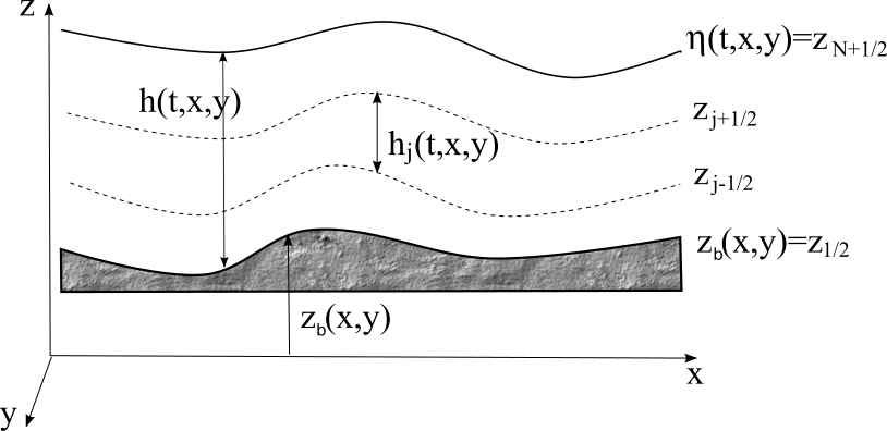
(a)	(b)

Figure 1: Fluid domain, notations and layerwise discretization.

3 The layer-averaged model

We consider a discretization of the fluid domain by layers (see Fig. 1-(b)) where the layer $\alpha$ contains the points of coordinates $(x,y,z)$ with $z\in L_{\alpha}(t,x,y)=[z_{\alpha-1/2},z_{\alpha+1/2}]$ and $\{z_{\alpha+1/2}\}_{\alpha=1,\ldots,N}$ is defined by

$$\left\{\begin{array}[]{l}z_{\alpha+1/2}(t,x,y)=z_{b}(x,y)+\sum_{j=1}^{\alpha}h_{j}(t,x,y),\\ h_{\alpha}(t,x,y)=z_{\alpha+1/2}(t,x,y)-z_{\alpha-1/2}(t,x,y)=l_{\alpha}h(t,x,y),\end{array}\right.$$ (15)

for $\alpha\in\{0,\ldots,N\}$ and $\sum_{\alpha=1}^{N}l_{\alpha}=1$.

3.1 The layer-averaged Euler system

The layer-averaging process for the 2d hydrostatic Euler and Navier-Stokes systems is precisely described in the paper [18] with a general rheology, the reader can refer to it. In the following, we present a Galerkin type approximation of the 3d Euler system also leading to a layer-averaged version of the Euler system, the obtained model reduces to [18] in the 2d context.

Using the notations (15), let us consider the space $\mathbb{P}_{0,h}^{N,t}$ of piecewise constant functions defined by

$$\mathbb{P}_{0,h}^{N,t}=\left\{{\bf 1}_{z\in L_{\alpha}(t,x,y)}(z),\quad\alpha\in\{1,\ldots,N\}\right\},$$ (16)

where ${\bf 1}_{z\in L_{\alpha}(t,x,y)}(z)$ is the characteristic function of the layer $L_{\alpha}(t,x,y)$. Using this formalism, the projection of $u$, $v$ and $w$ on $\mathbb{P}_{0,h}^{N,t}$ is a piecewise constant function defined by

$$X^{N}(t,x,y,z,\{z_{\alpha}\})=\sum_{\alpha=1}^{N}{\bf 1}_{[z_{\alpha-1/2},z_{\alpha+1/2}]}(z)X_{\alpha}(t,x,y),$$ (17)

for $X\in(u,v,w)$.

The three following propositions hold.

Proposition 3.1

Using the space $\mathbb{P}_{0,h}^{N,t}$ defined by (16) and the decomposition (17), the Galerkin approximation of the incompressible and hydrostatic Euler equations (12)-(13),(4),(5) leads to the system

$$\sum_{\alpha=1}^{N}\frac{\partial h_{\alpha}}{\partial t}+\sum_{\alpha=1}^{N}\nabla_{x,y}.(h_{\alpha}{\bf u}_{\alpha})=0,$$ (18)

$$\frac{\partial h_{\alpha}{\bf u}_{\alpha}}{\partial t}+\nabla_{x,y}.\left(h_{\alpha}{\bf u}_{\alpha}\otimes{\bf u}_{\alpha}\right)+\nabla_{x,y}\bigl{(}\frac{g}{2}hh_{\alpha}\bigr{)}=-gh_{\alpha}\nabla_{x,y}z_{b}$$

$$\hskip 56.9055pt+{\bf u}_{\alpha+1/2}G_{\alpha+1/2}-{\bf u}_{\alpha-1/2}G_{\alpha-1/2},\quad{\alpha}=1,...,N.$$ (19)

The quantity $G_{\alpha+1/2}$ (resp. $G_{\alpha-1/2}$) corresponds to mass exchange accross the interface $z_{\alpha+1/2}$ (resp. $z_{\alpha-1/2}$) and $G_{\alpha+1/2}$ is defined by

$$G_{\alpha+1/2} = \sum_{j=1}^{\alpha}\left(\frac{\partial h_{j}}{\partial t}+\nabla_{x,y}.(h_{j}{\bf u}_{j})\right)=-\sum_{j=1}^{N}\Bigl{(}\sum_{p=1}^{\alpha}l_{p}-{\bf 1}_{j\leq\alpha}\Bigr{)}\nabla_{x,y}.(h_{j}{\bf u}_{j}),$$ (20)

for $\alpha=1,\ldots,N$. The velocities at the interfaces ${\bf u}_{\alpha+1/2}$ are defined by

$${\bf u}_{\alpha+1/2}=\left\{\begin{array}[]{ll}{\bf u}_{\alpha}&\mbox{\rm if }\;G_{\alpha+1/2}\leq 0\\ {\bf u}_{\alpha+1}&\mbox{\rm if }\;G_{\alpha+1/2}>0\end{array}\right.$$ (21)

The smooth solutions of (18),(19) satisfy an energy balance and we have the following proposition.

Proposition 3.2

The system (18),(19) admits, for smooth solutions, the energy balance

$$\frac{\partial}{\partial t}E_{\alpha}+\nabla_{x,y}.\left({\bf u}_{\alpha}\left(E_{\alpha}+\frac{g}{2}h_{\alpha}h\right)\right)$$

$$\qquad=\left({\bf u}_{\alpha+1/2}.{\bf u}_{\alpha}-\frac{|{\bf u}_{\alpha}|^{2}-|{\bf u}_{\alpha+1}|^{2}}{2}\right)G_{\alpha+1/2}-\left({\bf u}_{\alpha-1/2}{\bf u}_{\alpha}-\frac{|{\bf u}_{\alpha}|^{2}-|{\bf u}_{\alpha-1}|^{2}}{2}\right)G_{\alpha-1/2},$$ (22)

with

$$E_{\alpha}=\frac{h_{\alpha}|{\bf u}_{\alpha}|^{2}}{2}+\frac{g}{2}h_{\alpha}h+gh_{\alpha}z_{b}.$$ (23)

The sum of Eqs. (22) for $\alpha=1,\ldots,N$ gives the energy balance

$$\frac{\partial}{\partial t}\sum_{\alpha=1}^{N}E_{\alpha}+\sum_{\alpha=1}^{N}\nabla_{x,y}.{\bf u}_{\alpha}\left(E_{\alpha}+\frac{g}{2}h_{\alpha}h\right)=-\sum_{\alpha=1}^{N-1}\frac{|{\bf u}_{\alpha+1/2}-{\bf u}_{\alpha}|^{2}}{2}|G_{\alpha+1/2}|.$$ (24)

Remark 3.1

Equation (24) is a layer discretization of the energy balance (11). The definition of ${\bf u}_{\alpha+1/2}$ given in (21) ensures the right hand side in Eq. (24) is nonpositive. Notice that a centered definition for ${\bf u}_{\alpha+1/2}$ i.e.

$${\bf u}_{\alpha+1/2}=\frac{{\bf u}_{\alpha}+{\bf u}_{\alpha+1}}{2},$$ (25)

instead of (21) leads to a vanishing right hand side in Eq. (24). But the centered choice (25) does not allow to obtain an energy balance in the variable density case and does not give a maximum principle, at the discrete level, see [16]. Simple calculations show that any other choice than (21) or (25) leads to a non negative r.h.s. in (24).

It is noticeable that, thanks to the kinematic boundary condition at each interface, the vertical velocity is no more a variable of the system (19). This is an advantage of this formulation over the hydrostatic model where the vertical velocity is needed in the momentum equation (2) and is deduced from the incompressibility condition (1). Even if the vertical velocity $w$ no more appears in the model (18)-(19), it can be obtained as follows.

Proposition 3.3

The piecewise constant approximation of the vertical velocity $w$ satifying Eq. (17) is given by

$$w_{\alpha}=k_{\alpha}-z_{\alpha}\nabla_{x,y}.{\bf u}_{\alpha}$$ (26)

with

$$k_{1} = \nabla_{x,y}.(z_{b}{\bf u}_{1}),\qquad k_{\alpha+1}=k_{\alpha}+\nabla_{x,y}.\bigl{(}z_{\alpha+1/2}({\bf u}_{\alpha+1}-{\bf u}_{\alpha})\bigr{)}.$$

The quantities $\{w_{\alpha}\}_{\alpha=1}^{N}$ are obtained only using a post-processing of the variables governing the system (18)-(19).

• Considering the divergence free condition (12), using the decomposition (17) and the space of test functions (16), we consider the quantity

  $$\int_{\mathbb{R}}{\bf 1}_{z\in L_{\alpha}(t,x,y)}\nabla.{\bf U}^{N}dz=0,$$

  with ${\bf U}^{N}=(u^{N},v^{N},w^{N})^{T}$. Simple computations give

  $$0=\int_{\mathbb{R}}{\bf 1}_{z\in L_{\alpha}(t,x,y)}\nabla.{\bf U^{N}}dz=\frac{\partial h_{\alpha}}{\partial t}+\frac{\partial}{\partial x}\int_{z_{\alpha-1/2}}^{z_{\alpha+1/2}}u\ dz+\frac{\partial}{\partial y}\int_{z_{\alpha-1/2}}^{z_{\alpha+1/2}}v\ dz-G_{\alpha+1/2}+G_{\alpha-1/2},$$

  leading to

  $$\frac{\partial h_{\alpha}}{\partial t}+\nabla_{x,y}.(h_{\alpha}{\bf u}_{\alpha})=G_{\alpha+1/2}-G_{\alpha-1/2},$$ (27)

  with $G_{\alpha\pm 1/2}$ defined by

  $$G_{\alpha+1/2}=\frac{\partial z_{\alpha+1/2}}{\partial t}+{\bf u}_{\alpha+1/2}.\nabla_{x,y}z_{\alpha+1/2}-w_{\alpha+1/2}.$$

  The sum for $\alpha=1,\ldots,N$ of the above relations gives Eq. (18) where the kinematic boundary conditions (4),(5) corresponding to

  $$G_{1/2}=G_{N+1/2}=0,$$ (28)

  have been used. Similarly, the sum for $j=1,\ldots,\alpha$ of the relations (27) with (28) gives the expression (20) for $G_{\alpha+1/2}$.

  Now we consider the Galerkin approximation of Eq. (13) i.e. the quantity

  $$\int_{\mathbb{R}}{\bf 1}_{z\in L_{\alpha}(t,x,y)}\left(\frac{\partial{\bf u}^{N}}{\partial t}+\nabla_{x,y}.({\bf u}^{N}\otimes{\bf u}^{N})+\frac{\partial{\bf u}^{N}w^{N}}{\partial z}+g\nabla_{x,y}\eta\right)dz=0,$$

  leading, after simple computations, to Eq. (19). $\blacksquare$

• In order to obtain (22) we multiply (27) by $g(h+z_{b})-|{\bf u}_{\alpha}|^{2}/2$ and (19) by ${\bf u_{\alpha}}$ then we perform simple manipulations. More precisely, the momentun equation along the $x$ axis multiplied by $u_{\alpha}$ gives

  $$\left(\frac{\partial}{\partial t}(h_{\alpha}u_{\alpha})+\frac{\partial}{\partial x}\left(h_{\alpha}u_{\alpha}^{2}+\frac{g}{2}hh_{\alpha}\right)+\frac{\partial}{\partial y}\left(h_{\alpha}u_{\alpha}v_{\alpha}\right)\right)u_{\alpha}=\\ \biggl{(}-gh_{\alpha}\frac{\partial z_{b}}{\partial x}+u_{\alpha+1/2}G_{\alpha+1/2}-u_{\alpha-1/2}G_{\alpha-1/2}\biggr{)}u_{\alpha}.$$

  Considering first the left hand side of the preceding equation excluding the pressure terms, we denote

  $$I_{u,\alpha}=\left(\frac{\partial}{\partial t}(h_{\alpha}u_{\alpha})+\frac{\partial}{\partial x}\left(h_{\alpha}u_{\alpha}^{2}\right)+\frac{\partial}{\partial y}\left(h_{\alpha}u_{\alpha}v_{\alpha}\right)\right)u_{\alpha},$$

  and using (27) we have

  $$I_{u,\alpha}=\frac{\partial}{\partial t}\left(\frac{h_{\alpha}u_{\alpha}^{2}}{2}\right)+\frac{\partial}{\partial x}\left(u_{\alpha}\frac{h_{\alpha}u_{\alpha}^{2}}{2}\right)+\frac{\partial}{\partial y}\left(v_{\alpha}\frac{h_{\alpha}u_{\alpha}^{2}}{2}\right)+\frac{u_{\alpha}^{2}}{2}\left(\frac{\partial h_{\alpha}}{\partial t}+\nabla_{x,y}.(h_{\alpha}{\bf u}_{\alpha})\right).$$

  Now we consider the contribution of the pressure terms over the energy balance i.e.

  $$I_{p,u,\alpha}=\left(\frac{\partial}{\partial x}\left(\frac{g}{2}hh_{\alpha}\right)+gh_{\alpha}\frac{\partial z_{b}}{\partial x}\right)u_{\alpha},$$

  and it comes

  $$I_{p,u,\alpha} = gh_{\alpha}\frac{\partial}{\partial x}(h+z_{b})u_{\alpha}=g\frac{\partial}{\partial x}\left(h_{\alpha}(h+z_{b})u_{\alpha}\right)-g(h+z_{b})\frac{\partial}{\partial x}(h_{\alpha}u_{\alpha})$$

  $$= \frac{\partial}{\partial x}\left(\left(\frac{g}{2}h_{\alpha}h+\frac{g}{2}h_{\alpha}(h+2z_{b})\right)u_{\alpha}\right)-g(h+z_{b})\frac{\partial}{\partial x}(h_{\alpha}u_{\alpha}).$$

  Performing the same manipulations over the momentum equation along $y$ and adding the terms $I_{u,\alpha}$,$I_{v,\alpha}$,$I_{p,u,\alpha}$,$I_{p,v,\alpha}$ and  (27) multiplied by $g(h+z_{b})$ gives the result. $\blacksquare$

• Using the boundary condition (4), an integration from $z_{b}$ to $z$ of the divergence free condition (1) easily gives

  $$w=-\nabla_{x,y}.\int_{z_{b}}^{z}{\bf u}\ dz.$$

  Replacing formally in the above equation ${\bf u}$ (resp. $w$) by ${\bf u}^{N}$ (resp. $w^{N}$) defined by (17) and performing an integration over the layer $L_{1}$ of the obtained relation yields

  $$h_{1}w_{1}=-\int_{z_{b}}^{z_{3/2}}\nabla_{x,y}.\int_{z_{b}}^{z}{\bf u}_{1}\ dzdz_{1}=h_{1}\nabla_{x,y}.(z_{b}{\bf u}_{1})-\frac{z_{3/2}^{2}-z_{b}^{2}}{2}\nabla_{x,y}.{\bf u}_{1},$$

  i.e. $w_{1}=\nabla_{x,y}.(z_{b}{\bf u}_{1})-z_{1}\nabla_{x,y}.{\bf u}_{1},$ corresponding to (26) for $\alpha=1$. A similar computation for the layers $L_{2},\ldots,L_{N}$ proves the result (26) for $\alpha=2,\ldots,N$. A more detailed version of this proof is given in [18]. $\blacksquare$

3.2 The layer-averaged Navier-Stokes system

In paragraph 3.1, we have applied the layer-averaging to the Euler system, we now use the same process for the hydrostatic Navier-Stokes system. First, we consider the Navier-Stokes system (1)-(7) for a Newtonian fluid and then with a simplified rheology.

3.2.1 Complete model

The layer-averaging process applied to the Navier-Stokes system (1)-(7) leads to the following proposition.

Proposition 3.4

The layer-averaged hydrostatic Navier-Stokes system (1)-(7) is given by

$$\sum_{\alpha=1}^{N}\frac{\partial h_{\alpha}}{\partial t}+\sum_{\alpha=1}^{N}\ \nabla_{x,y}.(h_{\alpha}{\bf u}_{\alpha})=0.$$ (29)

$$\frac{\partial h_{\alpha}{\bf u}_{\alpha}}{\partial t}+\ \nabla_{x,y}.\left(h_{\alpha}{\bf u}_{\alpha}\otimes{\bf u}_{\alpha}\right)+\nabla_{x,y}\bigl{(}\frac{g}{2}hh_{\alpha}\bigr{)}=-gh_{\alpha}\nabla_{x,y}z_{b}$$

$$+{\bf u}_{\alpha+1/2}G_{\alpha+1/2}-{\bf u}_{\alpha-1/2}G_{\alpha-1/2}+\nabla_{x,y}.\bigl{(}h_{\alpha}{\bf\Sigma}_{\alpha}\bigr{)}$$

$$-{\bf\Sigma}_{\alpha+1/2}\nabla_{x,y}z_{\alpha+1/2}+{\bf\Sigma}_{\alpha-1/2}\nabla_{x,y}z_{\alpha-1/2}$$

$$+2\nu_{\alpha+1/2}\frac{{\bf u}_{{\alpha}+1}-{\bf u}_{\alpha}}{h_{{\alpha}+1}+h_{\alpha}}-2\nu_{\alpha-1/2}\frac{{\bf u}_{\alpha}-{\bf u}_{{\alpha}-1}}{h_{\alpha}+h_{{\alpha}-1}}-\kappa_{\alpha}{\bf u}_{\alpha}+W_{\alpha}{\bf t}_{s},\quad{\alpha}=1,...,N,$$ (30)

with

$${\bf\Sigma}_{\alpha+1/2} = \begin{pmatrix}\Sigma_{xx,\alpha+1/2}&\Sigma_{xy,\alpha+1/2}\\ \Sigma_{yx,\alpha+1/2}&\Sigma_{yy,\alpha+1/2}\end{pmatrix},$$ (31)

$$\Sigma_{xx,\alpha+1/2} = \frac{\nu_{\alpha+1/2}}{h_{\alpha+1}+h_{\alpha}}\bigl{(}h_{\alpha}\frac{\partial u_{\alpha}}{\partial x}+h_{\alpha+1}\frac{\partial u_{\alpha+1}}{\partial x}\bigr{)}-2\nu_{\alpha+1/2}\frac{\partial z_{\alpha+1/2}}{\partial x}\frac{u_{\alpha+1}-u_{\alpha}}{h_{\alpha+1}+h_{\alpha}},$$ (32)

$$\Sigma_{xy,\alpha+1/2} = \frac{\nu_{\alpha+1/2}}{h_{\alpha+1}+h_{\alpha}}\bigl{(}h_{\alpha}\frac{\partial u_{\alpha}}{\partial y}+h_{\alpha+1}\frac{\partial u_{\alpha+1}}{\partial y}\bigr{)}-2\nu_{\alpha+1/2}\frac{\partial z_{\alpha+1/2}}{\partial y}\frac{u_{\alpha+1}-u_{\alpha}}{h_{\alpha+1}+h_{\alpha}},$$ (33)

$${\bf\Sigma}_{\alpha} = \begin{pmatrix}\Sigma_{xx,\alpha}&\Sigma_{xy,\alpha}\\ \Sigma_{yx,\alpha}&\Sigma_{yy,\alpha}\end{pmatrix}=\frac{{\bf\Sigma}_{\alpha+1/2}+{\bf\Sigma}_{\alpha-1/2}}{2},$$ (34)

and

$$\kappa_{\alpha}=\left\{\begin{array}[]{l}\kappa\quad{\rm if}\quad\alpha=1\\ 0\quad{\rm if}\quad\alpha\neq 1\end{array}\right.\quad\nu_{\alpha+1/2}=\left\{\begin{array}[]{l}0\quad{\rm if}\quad\alpha=0,N\\ \nu\quad{\rm if}\quad\alpha=1,...,N-1\\ \end{array}\right.\quad W_{\alpha}=\left\{\begin{array}[]{l}W\quad{\rm if}\quad\alpha=N\\ 0\quad{\rm if}\quad\alpha\neq N\\ \end{array}\right.$$ (35)

The vertical velocities $\{w_{\alpha}\}_{\alpha=1}^{N}$ are defined by (26).

For smooth solutions, the system (29)-(30) admits the energy balance

$$\frac{\partial}{\partial t}\sum_{\alpha=1}^{N}E_{\alpha} + \nabla_{x,y}.\sum_{\alpha=1}^{N}{\bf u}_{\alpha}\left(E_{\alpha}+\frac{g}{2}h_{\alpha}h-h_{\alpha}{\bf\Sigma}_{\alpha}\right)=-\sum_{\alpha=1}^{N-1}\frac{|{\bf u}_{\alpha+1/2}-{\bf u}_{\alpha}|^{2}}{2}|G_{\alpha+1/2}|$$ (36)

$$\qquad-\sum_{\alpha=1}^{N-1}\frac{h_{\alpha+1}+h_{\alpha}}{2\nu}{\bf\Sigma}_{\alpha+1/2}^{2}-\sum_{\alpha=1}^{N-1}2\nu\frac{|{\bf u}_{{\alpha}+1}-{\bf u}_{\alpha}|^{2}}{h_{{\alpha}+1}+h_{\alpha}}-\kappa|{\bf u}_{1}|^{2}+W{\bf u}_{N}.{\bf t}_{s},$$

with $E_{\alpha}$ defined by (23) and ${\bf\Sigma}_{\alpha+1/2}^{2}=\sum_{i,j}\Sigma_{i,j,\alpha+1/2}^{2}$. Relation (36) is consistent with a layer-averaged discretization of the equation (10).

Notice that in (36), we use the notation

$${\bf u}_{\alpha}{\bf\Sigma}_{\alpha}=\begin{pmatrix}u_{\alpha}{\bf\Sigma}_{xx,\alpha}+v_{\alpha}{\bf\Sigma}_{yx,\alpha}\\ u_{\alpha}{\bf\Sigma}_{xy,\alpha}+v_{\alpha}{\bf\Sigma}_{yy,\alpha}\end{pmatrix}.$$

• The proof is given in appendix A. $\blacksquare$

Remark 3.2

Notice that in the definition (34), since we consider viscous terms we use a centered approximation.

3.2.2 Simplified rheology

The viscous terms in the layer-averaged Navier-Stokes system are difficult to discretize especially when a discrete version of the energy balance has to be preserved. Hence, we propose a simplified version of the model given in prop. 3.4.

First, using simple manipulations, the viscous terms in the layer-averaged Navier-Stokes can be rewritten and Eq. (30) becomes

$$\frac{\partial h_{\alpha}{\bf u}_{\alpha}}{\partial t} \!\!\!\!\!\!\!\!+\nabla_{x,y}.\left(h_{\alpha}{\bf u}_{\alpha}\otimes{\bf u}_{\alpha}\right)+\nabla_{x,y}\bigl{(}\frac{g}{2}hh_{\alpha}\bigr{)}=-gh_{\alpha}\nabla_{x,y}z_{b}$$

$$+{\bf u}_{\alpha+1/2}G_{\alpha+1/2}-{\bf u}_{\alpha-1/2}G_{\alpha-1/2}+\nabla_{x,y}.\bigl{(}h_{\alpha}{\bf\Sigma}_{\alpha}^{0}\bigr{)}-{\bf T}_{\alpha}$$

$$+\Lambda_{\alpha+1/2}({\bf u}_{{\alpha}+1}-{\bf u}_{\alpha})-\Lambda_{\alpha-1/2}({\bf u}_{\alpha}-{\bf u}_{{\alpha}-1})-\kappa_{\alpha}{\bf u}_{\alpha}+W_{\alpha}{\bf t}_{s},\quad{\alpha}=1,...,N,$$

with

$$\Sigma_{xx,\alpha+1/2}^{0} = \frac{\nu_{\alpha+1/2}}{h_{\alpha+1}+h_{\alpha}}\bigl{(}h_{\alpha}\frac{\partial u_{\alpha}}{\partial x}+h_{\alpha+1}\frac{\partial u_{\alpha+1}}{\partial x}\bigr{)},$$ (37)

$$\Sigma_{xy,\alpha+1/2}^{0} = \frac{\nu_{\alpha+1/2}}{h_{\alpha+1}+h_{\alpha}}\bigl{(}h_{\alpha}\frac{\partial u_{\alpha}}{\partial y}+h_{\alpha+1}\frac{\partial u_{\alpha+1}}{\partial y}\bigr{)},$$ (38)

$$T_{x,\alpha+1/2} = 2\nu_{\alpha+1/2}\frac{\partial z_{\alpha+1/2}}{\partial x}\frac{\partial u_{\alpha+1}}{\partial x}+2\nu_{\alpha+1/2}\frac{\partial z_{\alpha+1/2}}{\partial y}\frac{\partial u_{\alpha+1}}{\partial y},$$ (39)

$$\Lambda_{\alpha+1/2} = 2\nu_{\alpha+1/2}\frac{1+|\nabla_{x,y}z_{\alpha+1/2}|^{2}}{h_{{\alpha}+1}+h_{\alpha}}-\nu_{\alpha+1/2}\nabla_{x,y}.\left(\frac{h_{\alpha}\nabla_{x,y}z_{\alpha+1/2}}{h_{{\alpha}+1}+h_{\alpha}}\right),$$ (40)

$${\bf T}_{\alpha+1/2} = \begin{pmatrix}T_{x,\alpha+1/2}\\ T_{y,\alpha+1/2}\end{pmatrix},\quad{\bf T}_{\alpha}=\begin{pmatrix}T_{x,\alpha}\\ T_{y,\alpha}\end{pmatrix}=\frac{{\bf T}_{\alpha+1/2}+{\bf T}_{\alpha-1/2}}{2},$$ (41)

$${\bf\Sigma}^{0}_{\alpha+1/2} = \begin{pmatrix}\Sigma_{xx,\alpha+1/2}^{0}&\Sigma_{xy,\alpha+1/2}^{0}\\ \Sigma_{yx,\alpha+1/2}^{0}&\Sigma_{yy,\alpha+1/2}^{0}\end{pmatrix},$$ (42)

$${\bf\Sigma}_{\alpha}^{0} = \begin{pmatrix}\Sigma_{xx,\alpha}^{0}&\Sigma_{xy,\alpha}^{0}\\ \Sigma_{yx,\alpha}^{0}&\Sigma_{yy,\alpha}^{0}\end{pmatrix}=\frac{{\bf\Sigma}_{\alpha+1/2}^{0}+{\bf\Sigma}_{\alpha-1/2}^{0}}{2}.$$ (43)

Considering a large number of layers i.e. $h_{\alpha}=l_{\alpha}h\rightarrow 0$ then the quantity $\Lambda_{\alpha+1/2}$ reduces to

$$\Gamma_{\alpha+1/2}=2\nu_{\alpha+1/2}\frac{1+|\nabla_{x,y}z_{\alpha+1/2}|^{2}}{h_{{\alpha}+1}+h_{\alpha}}.$$ (44)

Now let us examine the quantity ${\bf T}_{\alpha}$. Once the approximation has been made in (40) replacing it by (44), the only way for the layer-averaged model to satisfy an energy balance is to neglect the quantity ${\bf T}_{\alpha}$. The removal of the quantity ${\bf T}_{\alpha}$ is the mandatory counterpart of the valid approximation made in (40). Moreover, the first component of ${\bf T}_{\alpha}$ writes (for the sake of simplicity, we assume $1<\alpha<N$ and $h_{j}=h/N$, $\forall j$)

$$T_{x,\alpha} = -\frac{\nu}{2}\nabla_{x,y}z_{\alpha+1/2}.\nabla_{x,y}u_{\alpha+1}+\frac{\nu}{2}\nabla_{x,y}z_{\alpha-1/2}.\nabla_{x,y}u_{\alpha-1}$$

$$= -\frac{\nu}{2}\nabla_{x,y}z_{\alpha}.\nabla_{x,y}(u_{\alpha+1}-u_{\alpha-1})-\frac{\nu}{2}\nabla_{x,y}(u_{\alpha+1}+u_{\alpha-1}).\nabla_{x,y}h_{\alpha},$$

and considering smooth solutions (meaning $\frac{\partial u}{\partial z}$ is bounded) and a large value of $N$, we have

$$u_{\alpha+1}-u_{\alpha-1}\rightarrow 0,\quad h_{\alpha}\rightarrow 0,$$

and hence $T_{x,\alpha}$ can be neglected compared to the other rheology terms.

Remark 3.3

The approximations concerning the viscous terms ${\bf\Lambda}_{\alpha\pm 1/2}$ and ${\bf T}_{\alpha}$ can be explained geometrically as follows. The second term in (40) and the vector ${\bf T}_{\alpha}$ involve the quantities $\nabla_{x,y}z_{\alpha\pm 1/2}$ i.e. the gradient of the boundaries of each layer and arise from the layer averaging formulation. Except in few particular cases (equilibrium at rest with flat topography,…), when $N$ is small the two quantities $\nabla_{x,y}z_{\alpha-1/2}$ and $\nabla_{x,y}z_{\alpha+1/2}$ significantly differ (see Fig.1-(b)). Whereas for smooth solutions and $N$ large $\nabla_{x,y}z_{\alpha-1/2}\approx\nabla_{x,y}z_{\alpha+1/2}$ and the corresponding contributions in ${\bf\Lambda}_{\alpha\pm 1/2}$ and ${\bf T}_{\alpha}$ can be neglected.

So finally, with a simplified expression of the rheology terms, the layer-averaged hydrostatic Navier-Stokes system given in prop.3.4 becomes

$$\sum_{\alpha=1}^{N}\frac{\partial h_{\alpha}}{\partial t} \!\!\!\!\!\!\!\!+\sum_{\alpha=1}^{N}\ \nabla_{x,y}.(h_{\alpha}{\bf u}_{\alpha})=0,$$ (45)

$$\frac{\partial h_{\alpha}{\bf u}_{\alpha}}{\partial t} \!\!\!\!\!\!\!\!\!+\nabla_{x,y}.\left(h_{\alpha}{\bf u}_{\alpha}\otimes{\bf u}_{\alpha}\right)+\nabla_{x,y}\bigl{(}\frac{g}{2}hh_{\alpha}\bigr{)}=-gh_{\alpha}\nabla_{x,y}z_{b}$$ (46)

$$+{\bf u}_{\alpha+1/2}G_{\alpha+1/2}-{\bf u}_{\alpha-1/2}G_{\alpha-1/2}+\nabla_{x,y}.\bigl{(}h_{\alpha}{\bf\Sigma}_{\alpha}^{0}\bigr{)}$$

$$+\Gamma_{\alpha+1/2}({\bf u}_{{\alpha}+1}-{\bf u}_{\alpha})-\Gamma_{\alpha-1/2}({\bf u}_{\alpha}-{\bf u}_{{\alpha}-1})-\kappa_{\alpha}{\bf u}_{\alpha}+W_{\alpha}{\bf t}_{s},$$

with $\Sigma^{0}$ defined by (37),(38),(42) and (43). For smooth solutions, the system (45)-(46) admits the energy balance

$$\frac{\partial}{\partial t}\sum_{\alpha=1}^{N}E_{\alpha} + \nabla_{x,y}.\sum_{\alpha=1}^{N}{\bf u}_{\alpha}\left(E_{\alpha}+\frac{g}{2}h_{\alpha}h-h_{\alpha}{\bf\Sigma}_{\alpha}^{0}\right)$$ (47)

$$= -\sum_{\alpha=1}^{N-1}\frac{|{\bf u}_{\alpha+1/2}-{\bf u}_{\alpha}|^{2}}{2}|G_{\alpha+1/2}|$$

$$-\sum_{\alpha=1}^{N-1}\frac{h_{\alpha+1}+h_{\alpha}}{2\nu}({\bf\Sigma}_{\alpha+1/2}^{0})^{2}-\sum_{\alpha=1}^{N-1}\Gamma_{\alpha+1/2}|{\bf u}_{{\alpha}+1}-{\bf u}_{\alpha}|^{2}-\kappa|{\bf u}_{1}|^{2}+W{\bf u}_{N}.{\bf t}_{s}.$$

The proof of the energy balance (47) is similar to the one given in prop. 3.4.

Remark 3.4

The layer-averaged Navier-Stokes system defined by (45)-(46) has the form

$$\frac{\partial U}{\partial t}+\nabla_{x,y}.F(U)=S_{b}(U)+S_{e}(U,\partial_{t}U,\partial_{x}U)+S_{v,f}(U),$$ (48)

where $U=\left(h,q_{x,1},\ldots,q_{x,N},q_{y,1},\ldots,q_{y,N}\right)^{T}$, and

$$S_{b}(U)=\left(0,gh_{1}\frac{\partial z_{b}}{\partial x},\ldots,gh_{N}\frac{\partial z_{b}}{\partial x},gh_{1}\frac{\partial z_{b}}{\partial y},\ldots,gh_{N}\frac{\partial z_{b}}{\partial y}\right)^{T},$$

with $q_{x,\alpha}=h_{\alpha}u_{\alpha}$, $q_{y,\alpha}=h_{\alpha}v_{\alpha}$. We denote with $F(U)$ the fluxes of the conservative part, and with $S_{e}(U,\partial_{t}U,\partial_{x}U)$ and $S_{v,f}(U)$ the source terms, representing respectively the momentum exchanges and the viscous, wind and friction effects.

The numerical scheme for the system (48) will be given in Section 5.

4 Kinetic description for the Euler system

In this section we give a kinetic interpretation of the system (18)-(22). The numerical scheme for the system (18)-(19),(26) will be deduced from the kinetic description.

4.1 Preliminaries

We begin this section by recalling the classical kinetic approach – used in [29] for example – for the 1d Saint-Venant system

$$\begin{array}[]{l}\partial_{t}h+\partial_{x}(hu)=0,\\ \partial_{t}(hu)+\partial_{x}(hu^{2}+g\frac{h^{2}}{2})+gh\partial_{x}z_{b}=0,\end{array}$$ (49)

with the water depth $h(t,x)\geq 0$, the water velocity $u(t,x)\in\mathbb{R}$ and a slowly varying topography $z_{b}(x)$.

The kinetic Maxwellian is given by

$$M(U,\xi)=\frac{1}{g\pi}\Bigl{(}2gh-(\xi-u)^{2}\Bigr{)}_{+}^{1/2},$$ (50)

where $U=(h,hu)^{T}$, $\xi\in\mathbb{R}$ and $x_{+}\equiv\max(0,x)$ for any $x\in\mathbb{R}$. It satisfies the following moment relations,

$$\begin{array}[]{c}\int_{\mathbb{R}}\begin{pmatrix}1\\ \xi\end{pmatrix}M(U,\xi)\,d\xi=U,\qquad\int_{\mathbb{R}}\xi^{2}M(U,\xi)\,d\xi=hu^{2}+g\frac{h^{2}}{2}.\end{array}$$ (51)

These definitions allow us to obtain a kinetic representation of the Saint-Venant system.

Lemma 4.1

If the topography $z_{b}(x)$ is Lipschitz continuous, the pair of functions $(h,hu)$ is a weak solution to the Saint-Venant system (49) if and only if $M(U,\xi)$ satisfies the kinetic equation

$$\partial_{t}M+\xi\partial_{x}M-g(\partial_{x}z_{b})\partial_{\xi}M=Q,$$ (52)

for some “collision term” $Q(t,x,\xi)$ that satisfies, for a.e. $(t,x)$,

$$\int_{\mathbb{R}}Qd\xi=\int_{\mathbb{R}}\xi Qd\xi=0.$$ (53)

• If (52) and (53) are satisfied, we can multiply (52) by $(1,\xi)^{T}$, and integrate with respect to $\xi$. Using (51) and (53) and integrating by parts the term in $\partial_{\xi}M$, we obtain (49). Conversely, if $(h,hu)$ is a weak solution to (49), just define $Q$ by (52); it will satisfy (53) according to the same computations. $\blacksquare$

The standard way to use Lemma 53 is to write a kinetic relaxation equation [4, 30, 31], like

$$\partial_{t}f+\xi\partial_{x}f-g(\partial_{x}z_{b})\partial_{\xi}f=\frac{M-f}{\epsilon},$$ (54)

where $f(t,x,\xi)\geq 0$, $M=M(U,\xi)$ with $U(t,x)=\int(1,\xi)^{T}f(t,x,\xi)d\xi$, and $\epsilon>0$ is a relaxation time. In the limit $\epsilon\to 0$ we recover formally the formulation (52), (53). We refer to [30] for general considerations on such kinetic relaxation models without topography, the case with topography being introduced in [29]. Note that the notion of kinetic representation as (52), (53) differs from the so called kinetic formulations where a large set of entropies is involved, see [3]. For systems of conservation laws, these kinetic formulations include non-advective terms that prevent from writing down simple approximations. In general, kinetic relaxation approximations can be compatible with just a single entropy. Nevertheless this is enough for proving the convergence as $\varepsilon\to 0$, see [32].

4.2 Kinetic interpretation

In this paragaph, we give a kinetic interpretation of the model (18)-(19),(24).

To build the Gibbs equilibria, we choose the function

$$\chi_{0}(z_{1},z_{2})=\frac{1}{4\pi}{\bf 1}_{z_{1}^{2}+z_{2}^{2}\leq 4}.$$ (55)

This choice corresponds to the 2d version of the kinetic maxwellian used in 1d (see remark 4.2) and we have

$$M_{\alpha}=M(U_{\alpha},\xi,\gamma)=\frac{h_{\alpha}}{c^{2}}\chi_{0}\left(\frac{\xi-u_{\alpha}}{c},\frac{\gamma-v_{\alpha}}{c}\right),$$ (56)

with $c=\sqrt{\frac{g}{2}h}$

$$U_{\alpha}=(h_{\alpha},h_{\alpha}u_{\alpha},h_{\alpha}v_{\alpha})^{T},$$ (57)

and where $(\xi,\gamma)\in\mathbb{R}^{2}$. In other words, we have $M_{\alpha}=\frac{l_{\alpha}}{2g\pi}{\bf 1}_{(\xi-u_{\alpha})^{2}+(\gamma-v_{\alpha})^{2}\leq 2gh}$.

Remark 4.2

Starting from the 2d maxwellian in the single layer case i.e.

$$M_{sv}=\frac{1}{2g\pi}{\bf 1}_{(\xi-u)^{2}+(\gamma-v)^{2}\leq 2gh},$$ (58)

and computing its integral w.r.t. the variable $\gamma$ yields

$$\int_{\mathbb{R}}M_{sv}d\gamma=\int_{v-\sqrt{(2gh-(\xi-u)^{2})_{+}}}^{v+\sqrt{(2gh-(\xi-u)^{2})_{+}}}\frac{1}{2g\pi}d\gamma=\frac{1}{g\pi}\sqrt{(2gh-(\xi-u)^{2})_{+}},$$

that is exactly the expression (50).

The quantity $M_{\alpha}$ satisfies the following moment relations

$$\begin{array}[]{l}\displaystyle\int_{\mathbb{R}^{2}}\begin{pmatrix}1\\ \xi\\ \gamma\end{pmatrix}M(U_{\alpha},\xi,\gamma)\,d\xi d\gamma=\begin{pmatrix}h_{\alpha}\\ h_{\alpha}u_{\alpha}\\ h_{\alpha}v_{\alpha}\end{pmatrix},\quad\displaystyle\int_{\mathbb{R}^{2}}\begin{pmatrix}\xi^{2}\\ \xi\gamma\\ \gamma^{2}\end{pmatrix}M(U_{\alpha},\xi,\gamma)\,d\xi d\gamma=\begin{pmatrix}h_{\alpha}u_{\alpha}^{2}+g\frac{h_{\alpha}h}{2}\\ h_{\alpha}u_{\alpha}v_{\alpha}\\ h_{\alpha}v_{\alpha}^{2}+g\frac{h_{\alpha}h}{2}\end{pmatrix}.\end{array}$$ (59)

The interest of the function $\chi_{0}$ and hence the particular form (56) lies in its link with a kinetic entropy. Consider the kinetic entropy

$$H(f,\xi,\gamma,z_{b})=\frac{\xi^{2}+\gamma^{2}}{2}f+gz_{b}f,$$ (60)

where $f\geq 0$, $(\xi,\gamma)\in\mathbb{R}^{2}$, $z_{b}\in\mathbb{R}$. Then one can check the relations

$$\int_{\mathbb{R}^{2}}\begin{pmatrix}1\\ \xi\\ \gamma\end{pmatrix}H(M_{\alpha},\xi,\gamma)d\xi d\gamma=\begin{pmatrix}E_{\alpha}=\frac{h_{\alpha}}{2}(u_{\alpha}^{2}+v_{\alpha}^{2})+\frac{g}{2}h_{\alpha}(h+2z_{b})\\ u_{\alpha}(E_{\alpha}+\frac{g}{2}h_{\alpha}h)\\ v_{\alpha}(E_{\alpha}+\frac{g}{2}h_{\alpha}h).\end{pmatrix}$$ (61)

Let us introduce the Gibbs equilibria $N_{\alpha+1/2}$ defined by for $\alpha=0,\ldots,N$ by

$$N_{\alpha+1/2}=N(U_{\alpha+1/2},\xi)=\frac{G_{\alpha+1/2}}{c^{2}}\ \chi_{0}\left(\frac{\xi-u_{\alpha+1/2}}{c},\frac{\gamma-v_{\alpha+1/2}}{c}\right)\\ =\frac{G_{\alpha+1/2}}{g\pi h}{\bf 1}_{(\xi-u_{\alpha+1/2})^{2}+(\gamma-v_{\alpha+1/2})^{2}\leq 2gh}=\frac{G_{\alpha+1/2}}{h}M_{\alpha+1/2},$$ (62)

where $G_{\alpha+1/2}$ is defined by (20) and $u_{\alpha+1/2}$,$v_{\alpha+1/2}$ are given by (21). The quantity $N_{\alpha+1/2}$ satisfies the following moment relations

$$\int_{\mathbb{R}^{2}}\begin{pmatrix}1\\ \xi\\ \gamma\end{pmatrix}N_{\alpha+1/2}d\xi d\gamma=\begin{pmatrix}G_{\alpha+1/2}\\ u_{\alpha+1/2}G_{\alpha+1/2}\\ v_{\alpha+1/2}G_{\alpha+1/2}\end{pmatrix},\quad\int_{\mathbb{R}^{2}}\begin{pmatrix}\frac{\xi^{2}}{2}\\ \frac{\gamma^{2}}{2}\end{pmatrix}N_{\alpha+1/2}d\xi d\gamma=\begin{pmatrix}\left(\frac{u_{\alpha+1/2}^{2}}{2}+\frac{g}{4}h\right)G_{\alpha+1/2}\\ \left(\frac{v_{\alpha+1/2}^{2}}{2}+\frac{g}{4}h\right)G_{\alpha+1/2}\end{pmatrix}.$$ (63)

Notice that from (20), we can give a kinetic interpretation on the exchange terms under the form

$$G_{\alpha+1/2}=-\sum_{j=1}^{N}\Bigl{(}\sum_{p=1}^{\alpha}l_{p}-{\bf 1}_{j\leq\alpha}\Bigr{)}\int_{\mathbb{R}^{2}}\begin{pmatrix}\xi\\ \gamma\end{pmatrix}.\nabla_{x,y}M_{j}d\xi d\gamma,$$ (64)

for $\alpha=1,\ldots,N$.

Then we have the two following results.

Proposition 4.1

The functions ${\bf u}^{N}$ defined by (17) and $h$ are strong solutions of the system (18)-(19) if and only if the sets of equilibria $\{M_{\alpha}\}_{\alpha=1}^{N}$, $\{N_{\alpha+1/2}\}_{\alpha=0}^{N}$ are solutions of the kinetic equations defined by

$$({\cal B}_{\alpha})\qquad\frac{\partial M_{\alpha}}{\partial t}+\begin{pmatrix}\xi\\ \gamma\end{pmatrix}.\nabla_{x,y}M_{\alpha}-g\nabla_{x,y}z_{b}.\nabla_{\xi,\gamma}M_{\alpha}-N_{\alpha+1/2}+N_{\alpha-1/2}=Q_{\alpha},$$ (65)

for $\alpha=1,\ldots,N$. The quantities $Q_{\alpha}=Q_{\alpha}(t,x,y,\xi,\gamma)$ are “collision terms” equal to zero at the macroscopic level, i.e. they satisfy a.e. for values of $(t,x,y)$

$$\int_{\mathbb{R}^{2}}Q_{\alpha}d\xi d\gamma=\int_{\mathbb{R}^{2}}\xi Q_{\alpha}d\xi d\gamma=\int_{\mathbb{R}^{2}}\gamma Q_{\alpha}d\xi d\gamma=0.$$ (66)

Proposition 4.2

The solutions of (65) are entropy solutions if

$$\frac{\partial H(M_{\alpha})}{\partial t}+\begin{pmatrix}\xi\\ \gamma\end{pmatrix}.\nabla_{x,y}H(M_{\alpha})-g\nabla_{x,y}z_{b}.\nabla_{\xi,\gamma}H(M_{\alpha})\leq(H(N_{\alpha+1/2})-H(N_{\alpha-1/2})),$$ (67)

with the notation $H(M)=H(M,\xi,\gamma,z_{b})$ and $H$ defined by (60). The integration in $\xi,\gamma$ of relation (67) gives

$$\frac{\partial E_{\alpha}}{\partial t}+\nabla_{x,y}.{\bf u}_{\alpha}(E_{\alpha}+\frac{g}{2}h_{\alpha}h)\leq l_{\alpha}\left(\frac{|{\bf u}_{\alpha+1/2}|^{2}}{2}+gz_{b}\right)G_{\alpha+1/2}\\ -l_{\alpha}\left(\frac{|{\bf u}_{\alpha-1/2}|^{2}}{2}+gz_{b}\right)G_{\alpha-1/2}.$$

• The proof relies on averages w.r.t the variables $\xi,\gamma$ of Eq. (65) against the vector $(1,\xi,\gamma)^{T}$. Using relations (59),(62),(63) and the properties of the collision terms (66), the quantities

  $$\int_{\mathbb{R}^{2}}({\cal B}_{\alpha})\ d\xi d\gamma,\quad\int_{\mathbb{R}^{2}}\xi({\cal B}_{\alpha})\ d\xi d\gamma,\quad\mbox{and}\quad\int_{\mathbb{R}^{2}}\gamma({\cal B}_{\alpha})\ d\xi d\gamma,$$

  respectively give Eqs. (27) and (19). The sum for $\alpha=1$ to $N$ of Eqs. (27) with (20) gives (18) that completes the proof. $\blacksquare$

• The proof is obtained multiplying (65) by $H^{\prime}_{\alpha}(\overline{M}_{\alpha},\xi,\gamma,z_{b})$. Indeed, it is easy to see that

  $$H^{\prime}_{\alpha}(M_{\alpha},\xi,\gamma,z_{b})\frac{\partial M_{\alpha}}{\partial v}=\frac{\partial}{\partial v}H_{\alpha}(M_{\alpha},\xi,\gamma,z_{b}),$$

  for $v=t,x,y,\xi,\gamma$. Likewise for the quantity $H^{\prime}_{\alpha}(M_{\alpha},\xi,\gamma,z_{b})N_{\alpha+1/2}$, we have

  $$H^{\prime}_{\alpha}(M_{\alpha},\xi,\gamma,z_{b})N_{\alpha+1/2}=H(N_{\alpha+1/2},\xi,\gamma,z_{b}).$$

  So finally, Eq. (65) multiplied by $H^{\prime}_{\alpha}(M_{\alpha},\xi,\gamma,z_{b})$ gives

  $$\frac{\partial H_{\alpha}}{\partial t}+\begin{pmatrix}\xi\\ \gamma\end{pmatrix}.\nabla_{x,y}H_{\alpha}-g\nabla_{x,y}z_{b}.\nabla_{\xi,\gamma}H_{\alpha}\leq\left(\frac{\xi^{2}+\gamma^{2}}{2}+gz_{b}\right)(N_{\alpha+1/2}-N_{\alpha-1/2}).$$

  It remains to calculate the sum of the preceding relations from $\alpha=1,\ldots,N$ and to integrate the obtained relation in $\xi,\gamma$ over $\mathbb{R}^{2}$ that completes the proof. $\blacksquare$

Remark 4.3

If we introduce a $(2N+1)\times N$ matrix ${\cal K(\xi,\gamma)}$ defined by

$${\cal K}_{1,j}=1,\quad{\cal K}_{i+1,j}=\xi\delta_{i,j},\quad{\cal K}_{i+N+1,j+N}=\gamma\delta_{i,j},$$

for $i,j=1,\ldots,N$ with $\delta_{i,j}$ the Kronecker symbol. Then, using Prop. 66, we can write

$$U=\int_{\mathbb{R}^{2}}{\cal K(\xi,\gamma)}M(\xi,\gamma)d\xi d\gamma,\quad F(U)=\int_{\mathbb{R}^{2}}\begin{pmatrix}\xi\\ \gamma\end{pmatrix}{\cal K(\xi,\gamma)}M(\xi,\gamma)d\xi d\gamma,$$ (68)

$$S_{e}(U)=\int_{\mathbb{R}^{2}}{\cal K(\xi,\gamma)}N(\xi,\gamma)d\xi d\gamma,$$ (69)

with $M(\xi,\gamma)=(M(U_{1},\xi,\gamma),\ldots,M(U_{N},\xi,\gamma))^{T}$ and

$$N(\xi,\gamma)=\begin{pmatrix}N_{3/2}(\xi,\gamma)-N_{1/2}(\xi,\gamma)\\ \vdots\\ N_{N+1/2}(\xi,\gamma)-N_{N-1/2}(\xi,\gamma)\end{pmatrix}.$$

Hence, using the above notations, the layer-averaged Euler system (18)-(19) can be written under the form

$$\int_{\mathbb{R}^{2}}{\cal K}(\xi,\gamma)\left(\frac{\partial M(\xi,\gamma)}{\partial t}+\begin{pmatrix}\xi\\ \gamma\end{pmatrix}.\nabla_{x,y}M(\xi,\gamma)-g\nabla_{x,y}z_{b}.\nabla_{\xi,\gamma}M-N(\xi,\gamma)\right)d\xi d\gamma=0.$$

5 Numerical scheme

The numerical scheme for the model (48) proposed in this section extends the results presented by some of the authors in [33, 15, 16, 4]. Compared to these previous results, it has the following advantages

• it gives a 3d approximation of the Navier-Stokes system whereas 2d situations $(x,y)$ and $(x,z)$ where considered in [33, 15, 16],

• the implicit treatment of the vertical exchanges terms gives a bounded CFL condition even when the water depth vanishes,

• the kinetic interpretation, on which is based the numerical scheme, is also valid for the vertical exchange terms – that was not the case in [15, 16] – and allows to derive a robust and accurate numerical scheme,

• the numerical approximation of the system given in (48) is endowed with strong stability properties (well-balancing, positivity of the water depth,…),

• convergence curves towards a 3d non-stationary analytical solution with wet-dry interfaces have been obtained (see paragraph 6.2.1).

First, we focus on the Euler part of the system (48) then in paragraph 5.6, a numerical scheme for the viscous terms is proposed.

Notice that, as a consequence of the layer-averaged discretization, the system (48) and the Boltzmann type equation (65) are only 2d $(x,y)$ partial differential equations with source terms. Hence, the spacial approximation of the considered PDEs is performed on a 2d planar mesh.

5.1 Semi-discrete (in time) scheme

We consider discrete times $t^{n}$ with $t^{n+1}=t^{n}+\Delta t^{n}$. For the time discretisation of the layer-averaged Navier-Stokes system (48) we adopt the following scheme

$$U^{n+1}=U-\Delta t^{n}\left(\nabla_{x,y}.F(U)-S_{b}(U)\right)\\ +\Delta t^{n}S_{e}^{n+1}+\Delta t^{n}S_{v,f}^{n+p},$$ (70)

where the superscript ⁿ has been omitted and the integer $p=0,1/2,1$ will be precised below.

Using the expressions (45)-(46) for the layer averaged model, the semi-discrete in time scheme (70) writes

$$h^{n+1} = h^{n+1/2}=h-\Delta t^{n}\sum_{\alpha=1}^{N}\ \nabla_{x,y}.(h_{\alpha}{\bf u}_{\alpha}),$$ (71)

$$(h_{\alpha}{\bf u}_{\alpha})^{n+1/2} = h_{\alpha}{\bf u}_{\alpha}-\Delta t^{n}\Bigl{(}\nabla_{x,y}.\left(h_{\alpha}{\bf u}_{\alpha}\otimes{\bf u}_{\alpha}\right)+\nabla_{x,y}\bigl{(}\frac{g}{2}hh_{\alpha}\bigr{)}+gh_{\alpha}\nabla_{x,y}z_{b}\Bigr{)},$$ (72)

$$(h_{\alpha}{\bf u}_{\alpha})^{n+1} = (h_{\alpha}{\bf u}_{\alpha})^{n+1/2}-\Delta t^{n}\Bigl{(}{\bf u}_{\alpha+1/2}^{n+1}G_{\alpha+1/2}-{\bf u}_{\alpha-1/2}^{n+1}G_{\alpha-1/2}+\nabla_{x,y}.\bigl{(}h_{\alpha}^{n+p}{\bf\Sigma}_{\alpha}^{0,n+p}\bigr{)}$$ (73)

$$+\Lambda_{\alpha+1/2}\frac{{\bf u}_{{\alpha}+1}^{n+p}-{\bf u}_{\alpha}^{n+p}}{h_{{\alpha}+1}^{n+p}+h_{\alpha}^{n+p}}-\Lambda_{\alpha-1/2}\frac{{\bf u}_{\alpha}^{n+p}-{\bf u}_{{\alpha}-1}^{n+p}}{h_{\alpha}^{n+p}+h_{{\alpha}-1}^{n+p}}-\kappa_{\alpha}{\bf u}_{\alpha}^{n+p}+W_{\alpha}^{n+p}{\bf t}_{s}\Bigr{)},$$

$$G_{\alpha+1/2} = -\sum_{j=1}^{N}\Bigl{(}\sum_{p=1}^{\alpha}l_{p}-{\bf 1}_{j\leq\alpha}\Bigr{)}\nabla_{x,y}.(h_{j}{\bf u}_{j}),$$ (74)

for ${\alpha}=1,\ldots,N$. The vertical velocities $\{w_{\alpha}\}_{\alpha=1}^{N}$ are defined by (26). The first two equations(71)-(72) consist in an explicit time scheme where the horizontal fluxes and the topography source term are taken into account whereas in Eq. (73) an implicit treatment of the exchange terms between layers is proposed. The implicit part of the scheme requires to solve a linear problem (see lemma. 5.1) but, on the contrary of previous work of some of the authors [15], it implies that the CFL condition (100) no more depends on the exchange terms.

When $\nu=\kappa=0$ in Eq. (73), Eqs. (71)-(73) correspond to the layer-averaged of the Euler system. The choice $p=1$ (resp. $p=1/2$) in Eq. (73) corresponds to an implicit (resp. semi-implicit) treatment of the viscous and friction terms whereas the choice $p=0$ implies an explicit treatment and requires a CFL condition. Notice that the advantages and limitations of an implicit or explicit discretization in time scheme for the viscous and friction parts of Eq. (73) are not detailed here.

5.2 Space discretization

Let $\Omega$ denote the computational domain with boundary $\Gamma$, which we assume is polygonal. Let $T_{h}$ be a triangulation of $\Omega$ for which the vertices are denoted by $P_{i}$ with $S_{i}$ the set of interior nodes and $G_{i}$ the set of boundary nodes.

For the space discretization of the system(71)-(73), we use a finite volume technique for the Euler part – that is described below – and a finite element approach –$\mathbb{P}_{1}$ on $T_{h}$ – for the viscous part that is described in paragraph 5.6.

5.3 Finite volume formalism for the Euler part

In this paragraph and in paragraph (5.4), we propose a space discretization for the model (71)-(73) without the viscous and friction terms i.e. the system

$$h^{n+1} = h^{n+1/2}=h-\Delta t^{n}\sum_{\alpha=1}^{N}\nabla_{x,y}.(h_{\alpha}{\bf u}_{\alpha}),$$ (75)

$$(h_{\alpha}{\bf u}_{\alpha})^{n+1/2} = h_{\alpha}{\bf u}_{\alpha}-\Delta t^{n}\Bigl{(}\nabla_{x,y}.\left(h_{\alpha}{\bf u}_{\alpha}\otimes{\bf u}_{\alpha}\right)+\nabla_{x,y}\bigl{(}\frac{g}{2}hh_{\alpha}\bigr{)}+gh_{\alpha}\nabla_{x,y}z_{b}\Bigr{)},$$ (76)

$$(h_{\alpha}{\bf u}_{\alpha})^{n+1} = (h_{\alpha}{\bf u}_{\alpha})^{n+1/2}-\Delta t^{n}\Bigl{(}{\bf u}_{\alpha+1/2}^{n+1}G_{\alpha+1/2}-{\bf u}_{\alpha-1/2}^{n+1}G_{\alpha-1/2}\Bigr{)},$$ (77)

completed with (74).

We recall now the general formalism of finite volumes on unstructured meshes.

The dual cells $C_{i}$ are obtained by joining the centers of mass of the triangles surrounding each vertex $P_{i}$. We use the following notations (see Fig. 2):

• $K_{i}$, set of subscripts of nodes $P_{j}$ surrounding $P_{i}$,

• $|C_{i}|$, area of $C_{i}$,

• $\Gamma_{ij}$, boundary edge between the cells $C_{i}$ and $C_{j}$,

• $L_{ij}$, length of $\Gamma_{ij}$,

• ${\bf n}_{ij}$, unit normal to $\Gamma_{ij}$, outward to $C_{i}$ (${\bf n}_{ji}=-{\bf n}_{ij}$).

If $P_{i}$ is a node belonging to the boundary $\Gamma$, we join the centers of mass of the triangles adjacent to the boundary to the middle of the edge belonging to $\Gamma$ (see Fig. 2) and we denote

• $\Gamma_{i}$, the two edges of $C_{i}$ belonging to $\Gamma$,

• $L_{i}$, length of $\Gamma_{i}$ (for sake of simplicity we assume in the following that $L_{i}=0$ if $P_{i}$ does not belong to $\Gamma$),

• ${\bf n}_{i}$, the unit outward normal defined by averaging the two adjacent normals.

(a)	(b)

Figure 2: (a) Dual cell $C_{i}$ and (b) Boundary cell $C_{i}$.

We define the piecewise constant functions $U^{n}(x,y)$ on cells $C_{i}$ corresponding to time $t^{n}$ and $z_{b}(x,y)$ as

$$U^{n}(x,y)=U^{n}_{i},\quad z_{b}(x,y)=z_{b,i},\quad\mbox{ for }(x,y)\in C_{i},$$ (78)

with $U^{n}_{i}=(h^{n}_{i},q^{n}_{x,1,i},\ldots,q^{n}_{x,N,i},q^{n}_{y,1,i},\ldots,q^{n}_{y,N,i})^{T}$ i.e.

$$U^{n}_{i}\approx\frac{1}{|C_{i}|}\int_{C_{i}}U(t^{n},x,y)dxdy,\quad z_{b,i}\approx\frac{1}{|C_{i}|}\int_{C_{i}}z_{b}(x,y)dxdy.$$

We will also use the notation

$$U^{n}_{\alpha,i}\approx\frac{1}{|C_{i}|}\int_{C_{i}}U_{\alpha}(t^{n},x,y)dxdy,$$

with $U_{\alpha}$ defined by (57). A finite volume scheme for solving the system (75)-(76) is a formula of the form

$$U^{n+1/2}_{i}=U_{i}-\sum_{j\in K_{i}}\sigma_{i,j}\mathcal{F}_{i,j}-\sigma_{i}\mathcal{F}_{e,i},$$ (79)

where using the notations of (70)

$$\sum_{j\in K_{i}}L_{i,j}\mathcal{F}_{i,j}\approx\int_{C_{i}}\nabla_{x,y}.F(U)dxdy,$$ (80)

with

$$\sigma_{i,j}=\frac{\Delta t^{n}L_{i,j}}{|C_{i}|},\quad\sigma_{i}=\frac{\Delta t^{n}L_{i}}{|C_{i}|}.$$

Here we consider first-order explicit schemes where

$$\mathcal{F}_{i,j}=F(U_{i},U_{j},z_{b,i}-z_{b,j},{\bf n}_{i,j}).$$ (81)

and

$$\mathcal{F}_{i,j}=F(U_{i},U_{j},z_{b,i}-z_{b,j},{\bf n}_{i,j})=\begin{pmatrix}F(U_{1,i},U_{1,j},z_{b,i}-z_{b,j},{\bf n}_{i,j})\\ \vdots\\ F(U_{N,i},U_{N,j},z_{b,i}-z_{b,j},{\bf n}_{i,j})\end{pmatrix}$$ (82)

and for the boundary nodes

$$\mathcal{F}_{e,i}=F(U_{i},U_{e,i},{\bf n}_{i})=\begin{pmatrix}F(U_{1,i},U_{1,e,i},{\bf n}_{i})\\ \vdots\\ F(U_{N,i},U_{N,e,i},{\bf n}_{i})\end{pmatrix}.$$ (83)

Relation (79) tells how to compute the values $U^{n+1/2}_{i}$ knowing $U_{i}$ and discretized values $z_{b,i}$ of the topography. Following (80), the term $\mathcal{F}_{i,j}$ in (79) denotes an interpolation of the normal component of the flux $F(U).{\bf n}_{i,j}$ along the edge $C_{i,j}$. The functions $F(U_{i},U_{j},z_{b,i}-z_{b,j},{\bf n}_{i,j})\in\mathbb{R}^{2N+1}$ are the numerical fluxes, see [34].

In the next paragraph we define $\mathcal{F}(U_{i},U_{j},z_{b,i}-z_{b,j},{\bf n}_{i,j})$ using the kinetic interpretation of the system. The computation of the value $U_{i,e}$, which denotes a value outside $C_{i}$ (see Fig. 2-(b)), defined such that the boundary conditions are satisfied, and the definition of the boundary flux $F(U_{i},U_{e,i},{\bf n_{i}})$ are described paragraph 5.7. Notice that we assume a flat topography on the boundaries i.e. $z_{b,i}=z_{b,i,e}$.

5.4 Discrete kinetic equation

The choice of a kinetic scheme is motivated by several arguments. First, the kinetic interpretation is a suitable starting point for building a stable numerical scheme. We will prove in paragraph 5.4 that the proposed kinetic scheme preserves positivity of the water depth and ensures a discrete local maximum principle for a tracer concentration (temperature, salinity…). Second, the construction of the kinetic scheme does not need the computation of the system eigenvalues. This point is very important here since these eigenvalues are not available in explicit analytical form, and they are hardly accessible even numerically. Furthermore, as previously mentioned, hyperbolicity of the multilayer model may not hold, and the kinetic scheme allows overcoming this difficulty.

5.4.1 Without topography

In a first step we consider a situation with flat bottom. Following prop. 53, the model (18)-(19) reduces, for each layer, to a classical Saint-Venant system with exchange terms and its kinetic interpretation (see Eq. (65)) is given by

$$\frac{\partial M_{\alpha}}{\partial t}+\begin{pmatrix}\xi\\ \gamma\end{pmatrix}.\nabla_{x,y}M_{\alpha}-N_{\alpha+1/2}+N_{\alpha-1/2}=Q_{\alpha},\qquad\alpha\in\{1,\ldots,N\},$$ (84)

with the notations defined in paragraph 4.2.

Let $C_{i}$ be a cell, see Fig. 2. The integral over $C_{i}$ of the convective part of the kinetic equation (84) gives

$$\int_{C_{i}}\left(\frac{\partial M_{\alpha}}{\partial t}+\begin{pmatrix}\xi\\ \gamma\end{pmatrix}.\nabla_{x,y}M_{\alpha}\right)dxdy\approx|C_{i}|\frac{\partial M_{\alpha,i}}{\partial t}+\sum_{j\in K_{i}}\int_{\Gamma_{i,j}}M_{\alpha,i,j}dl,$$ (85)

with $M_{\alpha,i}=M(U_{\alpha,i},\xi,\gamma)$, ${\bf n}_{i,j}$ being the outward normal to the cell $C_{i}$. The quantity $M_{\alpha,i,j}$ is defined by the classical kinetic upwinding

$$M_{\alpha,i,j}=M_{\alpha,i}\zeta_{i,j}{\bf 1}_{\zeta_{i,j}\geq 0}+M_{\alpha,j}\zeta_{i,j}{\bf 1}_{\zeta_{i,j}\leq 0},$$

with $\zeta_{i,j}=\begin{pmatrix}\xi&\gamma\end{pmatrix}^{T}.{\bf n}_{i,j}$.

Therefore, the kinetic scheme applied for Eq.(84) is given by

$$f_{\alpha,i}^{n+1/2-} = \Bigl{(}1-\frac{\Delta t^{n}}{|C_{i}|}\sum_{j\in K_{i}}L_{i,j}\zeta_{i,j}{\bf 1}_{\zeta_{i,j}\geq 0}\Bigr{)}M_{\alpha,i}-\frac{\Delta t^{n}}{|C_{i}|}\sum_{j\in K_{i}}L_{i,j}M_{\alpha,j}\zeta_{i,j}{\bf 1}_{\zeta_{i,j}\leq 0},$$ (86)

$$f_{\alpha,i}^{n+1-} = f_{\alpha,i}^{n+1/2-}+\Delta t^{n}\Bigl{(}N_{\alpha+1/2,i}^{n+1-}-N_{\alpha-1/2,i}^{n+1-}\Bigr{)},$$ (87)

with the exchange terms $\{N_{\alpha+1/2,i}^{n+1-}\}_{\alpha=0}^{N}$ defined by

$$N_{\alpha+1/2,i}^{n+1-}(\xi,\gamma)=\frac{G_{\alpha+1/2,i}}{h_{i}}f_{\alpha+1/2,i}^{n+1-}.$$ (88)

Following (21) we can write

$$f_{\alpha+1/2,i}^{n+1-}=\left\{\begin{array}[]{ll}f_{\alpha,i}^{n+1-}&\mbox{\rm if }\;G_{\alpha+1/2}\leq 0\\ f_{\alpha+1,i}^{n+1-}&\mbox{\rm if }\;G_{\alpha+1/2}>0\end{array}\right.$$

leading to

$$N_{\alpha+1/2,i}^{n+1-}(\xi,\gamma)=\frac{|G_{\alpha+1/2,i}|_{+}}{h_{i}}f_{\alpha+1,i}^{n+1-}-\frac{|G_{\alpha+1/2,i}|_{-}}{h_{i}}f_{\alpha,i}^{n+1-}.$$

Notice that the previous definition is consistent with (62). From (64), we get

$$G_{\alpha+1/2,i}=-\frac{1}{|C_{i}|}\sum_{k=1}^{N}\Bigl{(}\sum_{p=1}^{\alpha}l_{p}-{\bf 1}_{k\leq\alpha}\Bigr{)}\sum_{j\in K_{i}}L_{i,j}\int_{\mathbb{R}^{2}}\left(M_{k,i}\zeta_{i,j}{\bf 1}_{\zeta_{i,j}\geq 0}+M_{k,j}\zeta_{i,j}{\bf 1}_{\zeta_{i,j}\leq 0}\right)d\xi d\gamma.$$

By analogy with the computations in (59), we can recover the macroscopic quantities $U_{\alpha,i}^{n+1}$ at time $t^{n+1}$ by integration of the relation (87)

$$U_{\alpha,i}^{n+1}=\int_{\mathbb{R}^{2}}\begin{pmatrix}1\\ \xi\\ \gamma\end{pmatrix}f_{\alpha,i}^{n+1-}d\xi d\gamma.$$ (89)

The scheme (86) and the definition (89) allow to complete the definition of the macroscopic scheme (79),(82), (83) with the numerical flux given by the flux vector splitting formula [31]

$$\mathcal{F}_{i,j} = F^{+}(U_{i}^{n},{\bf n}_{i,j})+F^{-}(U_{j}^{n},{\bf n}_{i,j})$$ (90)

$$= \int_{\mathbb{R}^{2}}{\cal K}(\xi,\gamma)M_{i}\zeta_{i,j}{\bf 1}_{\zeta_{i,j}\geq 0}d\xi d\gamma+\int_{\mathbb{R}^{2}}{\cal K}(\xi,\gamma)M_{j}\zeta_{i,j}{\bf 1}_{\zeta_{i,j}\leq 0}d\xi d\gamma,$$

where ${\cal K}(\xi,\gamma)$ is defined in Remark 4.3 and $M_{i}=(M_{1,i},\ldots,M_{N,i})^{T}$.

Using (88), we rewrite the step (87) under the form

$$\bigl{(}{\bf I}_{N}+\Delta t{\bf G}_{N,i}\bigr{)}f^{n+1-}=f^{n+1/2-},$$

where $I_{N}$ is the identity matrix of size $N$ and ${\bf G}_{N,i}$ is defined by

$$G_{N,i}=\begin{pmatrix}-\frac{|G_{3/2,i}|_{-}}{h_{1,i}^{n+1}}&-\frac{|G_{3/2,i}|_{+}}{h_{1,i}^{n+1}}&0&0&\cdots&0\\ \frac{|G_{3/2,i}|_{-}}{h_{2,i}^{n+1}}&\ddots&\ddots&0&\cdots&0\\ 0&\ddots&\ddots&\ddots&0&0\\ \vdots&0&\frac{|G_{\alpha-1/2,i}|_{-}}{h_{\alpha,i}^{n+1}}&-\frac{|G_{\alpha+1/2,i}|_{-}-|G_{\alpha-1/2,i}|_{+}}{h_{\alpha,i}^{n+1}}&-\frac{|G_{\alpha+1/2,i}|_{+}}{h_{\alpha,i}^{n+1}}&0\\ \vdots&\ddots&0&\ddots&\ddots&-\frac{|G_{N-1/2,i}|_{+}}{h_{N-1,i}^{n+1}}\\ 0&\cdots&0&0&\frac{|G_{N-1/2,i}|_{-}}{h_{N,i}^{n+1}}&\frac{|G_{N-1/2,i}|_{+}}{h_{N,i}^{n+1}}\end{pmatrix}.$$

Hence, the resolution of the discrete kinetic equation (87) requires to inverse the matrix

$$\begin{pmatrix}{\bf I}_{N}+\Delta t{\bf G}_{N,i}&0\\ 0&{\bf I}_{N}+\Delta t{\bf G}_{N,i}\end{pmatrix}$$

and we have the following lemma.

Lemma 5.1

The matrix ${\bf I}_{N}+\Delta t{\bf G}_{N,i}$

• is invertible for any $h_{i}^{n+1}>0$,

• $({\bf I}_{N}+\Delta t{\bf G}_{N,i})^{-1}$ has only positive coefficients,

• for any vector $T$ with non negative entries i.e. $T_{\alpha}\geq 0$, for $1\leq\alpha\leq N$, one has

  $$\|({\bf I}_{N}+\Delta t{\bf G}_{N,i})^{-t}T\|_{\infty}\leq\|T\|_{\infty}.$$

• (i) For any $h_{i}^{n+1}>0$, the matrix ${\bf I}_{N}+\Delta t{\bf G}_{N,i}$ is a strictly dominant diagonal matrix and hence it is invertible.

  (ii) Denoting ${\bf G}_{N,i}^{d}$ (resp. ${\bf G}_{N,i}^{nd}$) the diagonal (resp. non diagonal) part of ${\bf G}_{N,i}$ we can write

  $${\bf I}_{N}+\Delta t{\bf G}_{N,i}=({\bf I}_{N}+\Delta t{\bf G}_{N,i}^{d})\left({\bf I}_{N}-({\bf I}_{N}+\Delta t{\bf G}_{N,i}^{d})^{-1}(-\Delta tG_{N,i}^{nd})\right),$$

  where all the entries of the matrix ${\bf J}_{N,i}=({\bf I}_{N}+\Delta t{\bf G}_{N,i}^{d})^{-1}(-\Delta t{\bf G}_{N,i}^{nd})$, are non negative and less than 1. And hence, we can write

  $$({\bf I}_{N}+\Delta t{\bf G}_{N,i})^{-1}=\sum_{k=0}^{\infty}J_{N,i}^{k},$$

  proving all the entries of $({\bf I}_{N}+\Delta t{\bf G}_{N,i})^{-1}$ are non negative.

  (ii) Let us consider the vector ${\bf 1}$ whose entries are all equal to 1. Since we have

  $$({\bf I}_{N}+\Delta t{\bf G}_{N,i})^{t}{\bf 1}={\bf 1},$$

  we also have ${\bf 1}=({\bf I}_{N}+\Delta t{\bf G}_{N,i})^{-t}{\bf 1}$. Now let $T$ be a vector whose entries $\{T_{\alpha}\}_{1\leq\alpha\leq N}$ are non negative, then

  $$({\bf I}_{N}+\Delta t{\bf G}_{N,i})^{-t}{\bf T}\leq({\bf I}_{N}+\Delta t{\bf G}_{N,i})^{-t}{\bf 1}\|{\bf T}\|_{\infty}={\bf 1}\|{\bf T}\|_{\infty},$$

  that completes the proof. $\blacksquare$

5.4.2 With topography

The hydrostatic reconstruction scheme (HR scheme for short) for the Saint-Venant system has been introduced in [35] in the 1d case and described in 2d for unstructured meshes in [33]. The HR in the context of the kinetic description for the Saint-Venant system has been studied in [4].

In order to take into account the topography source and to preserve relevant equilibria, the HR leads to a modified version of (79) under the form

$$U^{n+1/2}_{i}=U^{n}_{i}-\sum_{j\in K_{i}}\sigma_{i,j}\mathcal{F}_{i,j}^{*}-\sigma_{i}\mathcal{F}_{i,e}+\sum_{j\in K_{i}}\sigma_{i,j}{\cal S}_{i,j}^{*},$$ (91)

where

$$\mathcal{F}^{*}_{i,j}=F(U_{i,j}^{*},U_{j,i}^{*},{\bf n}_{i,j}),\quad\mathcal{S}_{i,j}^{*}=S(U_{i},U_{i,j}^{*},{\bf n}_{i,j})=\begin{pmatrix}0\\ \frac{g}{2}l_{1}(h_{i,j}^{*2}-h_{i}^{2}){\bf n}_{i,j}\\ \vdots\\ \frac{g}{2}l_{N}(h_{i,j}^{*2}-h_{i}^{2}){\bf n}_{i,j}\end{pmatrix},$$ (92)

with

$$\begin{array}[]{l}z_{b,i,j}^{*}=\max(z_{b,i},z_{b,j}),\quad h_{i,j}^{*}=\max(h_{i}+z_{b,i}-z_{b,i,j}^{*},0),\\ U_{i,j}^{*}=(h_{i,j}^{*},l_{1}h_{i,j}^{*}u_{1,i},\ldots,l_{N}h_{i,j}^{*}u_{N,i},l_{1}h_{i,j}^{*}v_{1,i},\ldots,l_{N}h_{i,j}^{*}v_{N,i})^{T}.\end{array}$$ (93)

We would like here to propose a kinetic interpretation of the HR scheme, which means to interpret the above numerical fluxes as averages with respect to the kinetic variables of a scheme written on a kinetic function $f$. More precisely, we would like to approximate the solution to (65) by a kinetic scheme such that the associated macroscopic scheme is exactly (91)-(92) with homogeneous numerical flux $\mathcal{F}$ given by (90). We denote $M_{\alpha,i,j}^{*}=M(U_{\alpha,i,j}^{*},\xi,\gamma)$ for any $\alpha=1,\ldots,N$ and we consider the scheme

$$f_{\alpha,i}^{n+1/2-} = M_{\alpha,i}-\frac{\Delta t^{n}}{|C_{i}|}\sum_{j\in K_{i}}L_{i,j}\zeta_{i,j}{\bf 1}_{\zeta_{i,j}\geq 0}M_{\alpha,i,j}^{*}-\frac{\Delta t^{n}}{|C_{i}|}\sum_{j\in K_{i}}L_{i,j}M_{\alpha,j,i}^{*}\zeta_{i,j}{\bf 1}_{\zeta_{i,j}\leq 0},$$ (94)

$$-\frac{\Delta t^{n}}{|C_{i}|}\sum_{j\in K_{i}}L_{i,j}(M_{\alpha,i}-M_{\alpha,i,j}^{*})\theta_{\alpha,i,j},$$

$$f_{\alpha,i}^{n+1-} = f_{\alpha,i}^{n+1/2-}+\Delta t^{n}\Bigl{(}N_{\alpha+1/2,i}^{*,n+1-}-N_{\alpha-1/2,i}^{*,n+1-}\Bigr{)},$$ (95)

where

$$\theta_{\alpha,i,j}=\begin{pmatrix}\xi-u_{\alpha,i}\\ \gamma-v_{\alpha,i}\end{pmatrix}.{\bf n}_{i,j}.$$

For the exchange terms, by analogy with (88) we define

$$N_{\alpha+1/2,i}^{*,n+1-}(\xi,\gamma)=\frac{G_{\alpha+1/2,i}^{*}}{h_{i}}f_{\alpha+1/2,i}^{n+1-},$$ (96)

and using (64) we get

$$G_{\alpha+1/2,i}^{*}=-\frac{1}{|C_{i}|}\sum_{k=1}^{N}\Bigl{(}\sum_{p=1}^{\alpha}l_{p}-{\bf 1}_{k\leq\alpha}\Bigr{)}\sum_{j\in K_{i}}L_{i,j}\int_{\mathbb{R}^{2}}\left(M_{k,i,j}^{*}\zeta_{i,j}{\bf 1}_{\zeta_{i,j}\geq 0}+M_{k,i,j}^{*}\zeta_{i,j}{\bf 1}_{\zeta_{i,j}\leq 0}\right)d\xi d\gamma.$$

It is easy to see that in the previous formula, we have the moment relations

$$\int_{\mathbb{R}^{2}}(M_{\alpha,i}-M_{\alpha,i,j}^{*})\theta_{\alpha,i,j}d\xi d\gamma=0,$$ (97)

$$\int_{\mathbb{R}^{2}}\begin{pmatrix}\xi\\ \gamma\end{pmatrix}(M_{\alpha,i}-M_{\alpha,i,j}^{*})\theta_{\alpha,i,j}d\xi d\gamma=\frac{g}{2}l_{\alpha}(h_{i,j}^{*2}-h_{i}^{2}){\bf n}_{i,j},$$ (98)

Using again (89), the integration of the set of equations (94)-(95), for $\alpha=1,\ldots,N$, multiplied by ${\cal K}(\xi,\gamma)$ with respect to $\xi$,$\gamma$ then gives the HR scheme (91)-(92) with (90),(93). Thus as announced, (94)-(95) is a kinetic interpretation of the HR scheme in 3d for an unstructured mesh.

There exists a velocity $v_{m}\geq 0$ such that for all $\alpha,i$,

$$|\xi|\geq v_{m}\ \mbox{or }|\gamma|\geq v_{m}\Rightarrow M(U_{\alpha,i},\xi,\gamma)=0.$$ (99)

This means equivalently that $|u_{\alpha,i}|+|v_{\alpha,i}|+\sqrt{2gh_{i}}\leq v_{m}$. We consider a CFL condition strictly less than one,

$$\sigma_{i}v_{m}\leq\beta<\frac{1}{2}\quad\mbox{ for all }i,$$ (100)

where $\sigma_{i}=\Delta t^{n}\sum_{j\in K_{i}}L_{i,j}/|C_{i}|$, and $\beta$ is a given constant.

Then the following proposition holds.

Proposition 5.1

Under the CFL condition (100), the scheme (94)-(95) verifies the following properties.

(i) The macroscopic scheme derived from (94)-(95) using (89) is a consistent discretization of the layer-averaged Euler system (18)-(19).

(ii) The kinetic function remains nonnegative i.e.

$$f^{n+1-}_{\alpha,i}\geq 0,\qquad\forall(\xi,\gamma)\in\mathbb{R}^{2},\;\forall i,\ \forall\alpha.$$

(iii) The scheme (94)-(95) is kinetic well balanced i.e. at rest

$$f_{\alpha,i}^{n+1-}=M_{\alpha,i},\quad\forall(\xi,\gamma)\in\mathbb{R}^{2},\;\forall i,\ \forall\alpha=1,\ldots,N.$$ (101)

(i) Since the Boltzmann type equations (65) are almost linear transport equations with source terms, the discrete kinetic scheme (94)-(95) is clearly a consistent discretization of (65). And therefore using the kinetic interpretation given in prop. 66, the macroscopic scheme obtained from (94)-(95) using (89) is a consistent discretization of the layer-averaged Euler system (18)-(19).

(ii) In (94)-(95) we have

$$\frac{\Delta t^{n}}{|C_{i}|}\sum_{j\in K_{i}}L_{i,j}M_{\alpha,j,i}^{*}\zeta_{i,j}{\bf 1}_{\zeta_{i,j}\leq 0}\leq 0,$$

and the HR (93) ensures $M_{\alpha,i,j}^{*}\leq M_{\alpha,i}$, $\forall(\xi,\gamma)\in\mathbb{R}^{2},\forall\alpha$ leading to

$$f_{\alpha,i}^{n+1/2-}\geq\left(1-\frac{\Delta t^{n}}{|C_{i}|}\sum_{j\in K_{i}}L_{i,j}\bigl{(}\zeta_{i,j}{\bf 1}_{\zeta_{i,j}\geq 0}+\theta_{\alpha,i,j}{\bf 1}_{\theta_{\alpha,i,j}\geq 0}\bigr{)}\right)M_{\alpha,i},$$

But $\zeta_{i,j}{\bf 1}_{\zeta_{i,j}\geq 0}\leq\max\{|\xi|,|\gamma|\}$, $\theta_{\alpha,i,j}{\bf 1}_{\theta_{\alpha,i,j}\geq 0}\leq\max\{|\xi-u_{\alpha,i}|,|\gamma-v_{\alpha,i}|\}$ and therefore

$$\frac{\Delta t^{n}}{|C_{i}|}\sum_{j\in K_{i}}L_{i,j}\bigl{(}\zeta_{i,j}{\bf 1}_{\zeta_{i,j}\geq 0}+\theta_{\alpha,i,j}{\bf 1}_{\theta_{\alpha,i,j}\geq 0}\bigr{)}\leq\sigma_{i}(\max\{|\xi|,|\gamma|\}+\max\{|\xi-u_{\alpha,i}|,|\gamma-v_{\alpha,i}|\})\leq 1,$$

where (99),(100) have been used, proving $f_{\alpha,i}^{n+1/2-}\geq 0$ for any $\xi\in\mathbb{R}$ and any $\alpha\in\{1,\ldots,N\}$. Now using the results of lemma 5.1, it ensures that $f_{\alpha,i}^{n+1-}$ defined by (95) satisfies $f_{\alpha,i}^{n+1-}\geq 0$ for any $(\xi,\gamma)\in\mathbb{R}^{2}$ and any $\alpha\in\{1,\ldots,N\}$, proving (ii).

(iii) Considering the situation at rest i.e. $u_{\alpha,i}=v_{\alpha,i}=0$, $\forall\alpha,i$ and $h_{i}+z_{b,i}=h_{j}+z_{b,j}$, $\forall i,j$ we have

$$M_{\alpha,i}=M_{\alpha,i,j}^{*},\qquad\forall\alpha,i,j.$$

From (94)-(95), this gives (101). $\blacksquare$

5.5 Macroscopic scheme

The numerical scheme for the system (75)-(77) is given by (89),(94), (95) and requires to calculate fluxes having the form

$$F_{sv}(U) = \left(\begin{array}[]{c}F_{h}\\ F_{hu}\\ F_{hv}\end{array}\right)=\int_{n_{x}\xi+n_{y}\gamma\geq 0}\left(\begin{array}[]{c}1\\ \xi\\ \gamma\end{array}\right)(n_{x}\xi+n_{y}\gamma)M(U,\xi,\gamma)d\xi d\gamma.$$

with $M$ given by (58), $n_{x}$ and $n_{y}$ being the components of a normal unit vector ${\bf n}$. Defining the change of variables

$$\xi=u+cz_{1},\qquad\gamma=v+cz_{2},$$

we can write

$$F_{sv}(U)=h\int_{n_{x}(cz_{1}+u)+n_{y}(cz_{2}+v)\geq 0}(n_{x}(cz_{1}+u)+n_{y}(cz_{2}+v))\left(\begin{array}[]{c}1\\ u+cz_{1}\\ v+cz_{2}\end{array}\right)\chi_{0}(z_{1},z_{2})dz_{1}dz_{2},$$

where $\chi_{0}$ is defined by (55). A second change of variables $y_{1}=n_{x}z_{1}+n_{y}z_{2}$, $y_{2}=n_{x}z_{2}-n_{y}z_{1}$, $\tilde{u}=n_{x}u+n_{y}v$ gives

$$F_{sv}(U)=h\int_{\{y_{1}\geq-\frac{\tilde{u}}{c}\}\times\mathbb{R}}(\tilde{u}+cy_{1})\left(\begin{array}[]{c}1\\ u+cn_{x}y_{1}\\ v+cn_{y}y_{1}\end{array}\right)\chi_{0}(y_{1},y_{2})dy_{1}dy_{2},$$ (103)

since $\chi_{0}$ is odd. The details of the computations of formula (103) is given in appendix B.

Using the properties obtained at the kinetic level for the resolution of the system (18)-(19), the following proposition holds.

Proposition 5.2

Under the CFL condition (100), the scheme (89),(94), (95) satisfies the following properties.

(i) The macroscopic scheme derived from (94)-(95) using (89) is a consistent discretization of the layer-averaged Euler system (18)-(19).

(ii) The water depth remains nonnegative i.e.

$$h^{n+1}_{i}\geq 0,\quad\forall i,\quad\mbox{when}\;h^{n}_{i}\geq 0\quad\forall i.$$

(iii) The scheme (89),(94), (95) is well-balanced.

• The proof is similar to the one given in prop. 101. $\blacksquare$

5.6 The discrete layer-averaged Navier-Stokes system

In this paragraph, we detail the space discretization of the viscous terms. Several expressions have been obtained for the viscous terms, see paragraph 3.2. In this paragraph, we give a numerical scheme for the model (73), rewriting it under the form

$$(h_{\alpha}{\bf u}_{\alpha})^{n+1}=\widetilde{h_{\alpha}{\bf u}_{\alpha}}+\Delta t^{n}S_{v,f}(U),$$ (104)

with $S_{v,f}(U)=(S_{v,f,1},\ldots,S_{v,f,N})^{T}$ and

$$\widetilde{h_{\alpha}{\bf u}_{\alpha}} = h_{\alpha}{\bf u}_{\alpha}-\Delta t^{n}\Bigl{(}\nabla_{x,y}.\left(h_{\alpha}{\bf u}_{\alpha}\otimes{\bf u}_{\alpha}\right)-\nabla_{x,y}\bigl{(}\frac{g}{2}hh_{\alpha}\bigr{)}-gh_{\alpha}\nabla_{x,y}z_{b}$$

$$+{\bf u}_{\alpha+1/2}^{n+1}G_{\alpha+1/2}-{\bf u}_{\alpha-1/2}^{n+1}G_{\alpha-1/2}\Bigr{)},$$

$$S_{v,f,\alpha} = \nabla_{x,y}.\bigl{(}h_{\alpha}{\bf\Sigma}_{\alpha}^{0}\bigr{)}+\Gamma_{\alpha+1/2}({\bf u}_{{\alpha}+1}-{\bf u}_{\alpha})-\Gamma_{\alpha-1/2}({\bf u}_{\alpha}-{\bf u}_{{\alpha}-1})-\kappa_{\alpha}{\bf u}_{\alpha}+W_{\alpha}{\bf t}_{s},$$

with the definitions (37),(38),(42), (43),(44) for ${\bf T}^{0}_{\alpha}$, $\Gamma_{\alpha\pm 1/2}$. It remains to give a fully discrete scheme for the viscous and friction terms $\{S_{v,f,\alpha}\}$.

The discretization of (104) is done using a finite element / finite difference approximation obtained as follows. We depart form the triangulation defined in paragraph (5.2) and we use the cells values of the variables – inherited from the finite volume framework – to define a $\mathbb{P}_{1}$ approximation of the variables.

Notice that, compared to the advection and pressure terms, the discretization of the viscous terms raises less difficulties and we propose a stable scheme that will be extended to more general rheology terms [18] and more completely analyzed in a forthcoming paper.

Using a classical $\mathbb{P}_{1}$ finite element type approximation with mass lumping of Eq. (104), we get

$${\bf U}_{\alpha}^{n+1} = \widetilde{{\bf U}}_{\alpha}-\Delta t^{n}\Bigl{(}{\cal K}_{\alpha+1}{\bf U}_{\alpha+1}+{\cal K}_{\alpha}{\bf U}_{\alpha}+{\cal K}_{\alpha-1}{\bf U}_{\alpha-1}\Bigr{)}$$ (105)

$$+\Delta t^{n}{\cal G}_{\alpha+1/2}({\bf U}_{\alpha+1}-{\bf U}_{\alpha})-\Delta t^{n}{\cal G}_{\alpha-1/2}({\bf U}_{\alpha}-{\bf U}_{\alpha-1})-\Delta t^{n}\kappa_{\alpha}{\bf U}_{\alpha}+\Delta t^{n}W_{\alpha}{\bf t}_{s},$$

with the matrices

$${\cal K}_{\alpha,ji} = \frac{\nu}{2}\int_{\Omega}\left(\frac{h_{\alpha,j}}{h_{\alpha+1,j}+h_{\alpha,j}}+\frac{h_{\alpha,j}}{h_{\alpha,j}+h_{\alpha-1,j}}\right)\nabla_{x,y}\varphi_{i}.\nabla_{x,y}\varphi_{j}\ dxdy,$$

$${\cal K}_{\alpha\pm 1,ji} = \frac{\nu_{\alpha\pm 1/2}}{2}\int_{\Omega}\frac{h_{\alpha\pm 1,j}}{h_{\alpha+1,j}+h_{\alpha,j}}\nabla_{x,y}\varphi_{i}.\nabla_{x,y}\varphi_{j}\ dxdy,$$

$${\cal G}_{\alpha+1/2,ji} = \nu_{\alpha+1/2}\int_{\Omega}\frac{1+|\nabla_{x,y}z_{\alpha+1/2}|^{2}}{h_{{\alpha}+1}+h_{\alpha}}\varphi_{i}.\varphi_{j}dxdy,$$

where $\varphi_{i}$, $\varphi_{j}$ are the basis functions. We have presented an explicit in time version of (105) that is stable under a classical CFL condition. An implicit or semi-implicit version of (105) can also be used.

The main purpose of this paper is to propose a stable and robust numerical approximation of the incompressible Euler system with free surface. Voluntarily, we give few details concerning the numerical approximation of the dissipative terms:

• the viscous and friction terms are dissipative and hence a reasonable approximation leads to a stable numerical scheme.

• In this paper, we consider a simplified Newtonian rheology for the fluid, the numerical approximation of the general (layer-averaged) rheology [18] will be studied in a forthcoming paper.

5.7 Boundary conditions

The contents of this paragraph slightly differ from previous works of one of the authors [36] and valid for the classical Saint-Venant system. First, we focus on the boundary conditions for the layer-averaged Euler system i.e. the system (71)-(72) for $\nu=0$, $\kappa=0$ and then for the viscous part.

5.7.1 Layer-averaged Euler system

In this paragraph we detail the computation of the boundary flux ${\cal F}({\bf U}_{i},{\bf U}_{e,i},{\bf n}_{i})$ appearing in (79),(82),(83). The variable ${\bf U}_{i,e}^{n}$ can be interpreted as an approximation of the solution in a ghost cell adjacent to the boundary. As before we introduce the vector

$$U_{i,e}=\left(h_{i,e}^{n},(hu)_{1,i,e},\ldots,(hu)_{N,i,e},(hv)_{1,i,e},\ldots,(hv)_{N,i,e}\right)^{T},$$

and we will use the flux vector splitting form associated to the kinetic formulation (90)

$${\cal F}(U_{i},U_{i,e},{\bf n}_{i})=F^{+}(U_{i},{\bf n}_{i})+F^{-}(U_{i,e},{\bf n}_{i})$$ (106)

with $U_{i,e}^{n}$ defined according to the boundary type.

Solid wall

If we consider a node $i_{0}$ belonging to a solid wall, we prescribe a slip condition written

$${\bf u}_{\alpha}\cdot{\bf n}_{i_{0}}=0,$$ (107)

for $\alpha=1,\ldots,N$. We assume the continuity of the water depth $h_{i_{0},e}=h_{i_{0}}$ and of the tangential component of velocity.

From (103) with (107) we obtain

$$F_{h}^{+}(U_{\alpha,i_{0}})+F_{h}^{-}(U_{\alpha,i_{0},e})=0,$$

and

$$\begin{pmatrix}F_{hu}^{+}(U_{\alpha,i_{0}})+F_{hu}^{-}(U_{\alpha,i_{0},e})\\ F_{hv}^{+}(U_{\alpha,i_{0}})+F_{hv}^{-}(U_{\alpha,i_{0},e})\end{pmatrix}.{\bf n}_{i_{0}}=\frac{gh_{\alpha,i_{0}}h_{i_{0}}}{2},\quad\begin{pmatrix}F_{hu}^{+}(U_{\alpha,i_{0}})+F_{hu}^{-}(U_{\alpha,i_{0},e})\\ F_{hv}^{+}(U_{\alpha,i_{0}})+F_{hv}^{-}(U_{e,\alpha,i_{0}})\end{pmatrix}.{\bf t}_{i_{0}}=0,$$

for $\alpha=1,\ldots,N$ for a vector ${\bf t}_{i_{0}}$ orthogonal to ${\bf n}_{i_{0}}$. The condition (107) is therefore prescribed weakly but a posteriori, in order to be sure that (107) is satisfied, we can apply

$${\bf u}_{\alpha,i_{0},e}={\bf u}_{\alpha,i_{0}}-({\bf u}_{\alpha,i_{0}}.{\bf n}_{i_{0}}){\bf n}_{i_{0}}.$$

Fluid boundary

Even if the considered model is more complex than the Shallow water system, we can consider that the type of the flow depends, for each layer, on the value of the Froud number $Fr_{\alpha}=|{\bf u}_{\alpha}|/\sqrt{gh}$, a flow is said torrential, for $|{\bf u}_{\alpha}|>\sqrt{gh}$ and fluvial, for $|{\bf u}_{\alpha}|<\sqrt{gh}$.

Generally, for the fluid boundaries, the conditions prescribed by the user depend on the type of the flow defined by this criterion.

We have also to notice that with ${\bf n}$ the outward unit normal to the boundary edge, an inflow boundary corresponds to ${\bf u}_{\alpha}\cdot{\bf n}<0$ and an outflow one to ${\bf u}_{\alpha}\cdot{\bf n}>0$.

We will treat the following cases: for a fluvial flow boundary, we distinguish the cases where the flux or the water depth are given, while for a torrential flow we distinguish the inflow or outflow boundaries.

Fluvial boundary. Flux given

We consider first a fluvial boundary, so we assume that

$$|{\bf u}_{\alpha}|<\sqrt{gh}.$$ (108)

If for each layer, the flux ${\bf q}_{g,\alpha}$ is given, then we wish to impose

$$\left(F_{h}({\bf U}_{\alpha,i})+F_{h}({\bf U}_{e,\alpha,i})\right).{\bf n}_{i}={\bf q}_{g,\alpha}.{\bf n}_{i},\quad F_{h}({\bf U}_{e,\alpha,i}).{\bf t}_{i}=q_{g,\alpha}.{\bf t}_{i},\\$$ (109)

with ${\bf n}_{i}.{\bf t}_{i}=0$. The value ${\bf q}_{g,\alpha}$ depends on the value of the prescribed flux along the vertical axis.

If one directly imposes (109), it leads to instabilities (especially because the numerical values are not necessarily in the regime of validity of this condition). We propose to discretize it in a weak form. We denote

$$a_{1}={\bf q}_{g,\alpha}.{\bf n}_{i}-F_{h}({\bf U}_{\alpha,i}).{\bf n}_{i}.$$ (110)

If $a_{1}\geq 0$, we prescribe

$$F_{h}({\bf U}_{e,\alpha,i})=0,\quad F_{hu}({\bf U}_{e,\alpha,i})=0,\quad\mbox{and}\quad F_{hv}({\bf U}_{e,\alpha,i})=0.$$

If $a_{1}<0$, we have to write a third equation to be able to compute the three components of ${\bf U}_{e,\alpha}$ and by analogy with what is done for the Saint-Venant system – where the Riemann invariant related to the outgoing characteristic is preserved – we assume the quantity ${\bf u}_{\alpha}.{\bf n}$ is constant though the interface, i.e.

$${\bf u}_{e,\alpha,i}.{\bf n}_{i}-2\sqrt{gh_{e,i}}={\bf u}_{\alpha,i}.{\bf n}_{i}-2\sqrt{gh_{i}}.$$ (111)

As (108) is satisfied, the eigenvalue $u_{e,\alpha,i}.{\bf n}_{i}-2\sqrt{gh_{e,i}}$ is positive.

We use the equations (109) and (111) to compute $h_{e,i}$ and ${\bf u}_{e,\alpha,i}.{\bf n}_{i}$. We denote $a_{2}={\bf u}_{\alpha,i}.{\bf n}_{i}-2\sqrt{gh_{i}}$ and

$$m=\frac{{\bf u}_{e,\alpha,i}.{\bf n}_{i}}{\sqrt{gh_{e,i}}}.$$ (112)

Then the equation (111) gives

$$\sqrt{gh_{e,i}}\ (m-2)=a_{2}$$ (113)

and using the definition of $F_{h}$ (see (134)) with (109),(110) we have

$$\frac{h_{e,i}}{\pi}\int_{z\leq\frac{-{\bf u}_{e,\alpha,i}.{\bf n}_{i}}{\sqrt{\frac{gh_{e,i}}{2}}}}\left({\bf u}_{e,\alpha,i}.{\bf n}_{i}+\sqrt{\frac{gh_{e,i}}{2}}z\right)\sqrt{1-\frac{z^{2}}{4}}dz=a_{1},$$ (114)

or using (111)

$$\psi(h_{e,i})=a_{1},$$ (115)

with

$$\psi(h_{e,i})=\frac{h_{e,i}}{\pi}\int_{z\leq\,\frac{-(2\sqrt{gh_{e,i}}+a_{2})}{\sqrt{\frac{gh_{e,i}}{2}}}}\left(2\sqrt{gh_{e,i}}+a_{2}+\sqrt{\frac{gh_{e,i}}{2}}z\right)\sqrt{1-\frac{z^{2}}{4}}dz.$$

It is easy to see that $h\mapsto\psi(h)$ is a growing function of $h$ with $\psi(0)=0$ and $\psi(+\infty)=+\infty$ and therefore, Eq. (114) admits a unique solution for any $a_{1}>0$. Using (113), Eq. (115) is equivalent to solve for $m$

$$\Psi(m)=a_{2},$$ (116)

with

$$\Psi(m)=K\frac{m-2}{\phi(m)^{1/3}},$$

and $K=\bigl{(}{\sqrt{2}ga_{1}}\bigr{)}^{1/3}$

$$\phi(m)=\frac{1}{\pi}\int_{z\leq-\sqrt{2}m}(\sqrt{2}m+z)\sqrt{1-\frac{z^{2}}{4}}dz.$$

In practice, we use a Newton-Raphson algorithm to solve an equivalent form of Eq. (116), namely

$$m-2-\frac{a_{2}}{K}\phi(m)^{1/3}=0.$$

Once the above equation has been solved, from (112),(113) we deduce

$$h_{e,i}=\frac{1}{g}\bigl{(}\frac{a_{2}}{m-2}\bigr{)}^{2},\quad{\bf u}_{e,\alpha,i}.{\bf n}_{i}=\frac{a_{2}m}{m-2}=m\sqrt{gh_{e,i}}.$$

Remark 5.2

Notice that in the procedure proposed to calculate ${\bf u}_{e,\alpha,i}$, $h_{e,i}$, even if $h_{e,i}$ represents a total water depth, a different value of $h_{e,i}$ is calculated for each layer $\alpha$. $h_{e,i}$ is only used to ensure (109).

Fluvial boundary. Water depth given

We verify that the flow is actually fluvial, i.e.

$$({\bf u}_{\alpha,i}.{\bf n}_{i}-\sqrt{gh}_{i})({\bf u}_{\alpha,i}.{\bf n}_{i}+\sqrt{gh}_{i})\leq 0.$$ (117)

Since the water depth is given, we write

$$h_{e,i}=h_{g,i}.$$ (118)

We assume the continuity of the tangential component

$$(h{\bf u})_{e,\alpha,i}.{\bf t}_{i}=(h{\bf u})_{\alpha,i}.{\bf t}_{i},$$ (119)

with ${\bf t}_{i}.{\bf n}_{i}=0$. To define completely ${\bf u}_{e,\alpha,i}$, we assume, as in the previous case, that the Riemann invariant is constant along the outgoing characteristic (111), so we obtain

$${\bf u}_{e,\alpha,i}.{\bf n}_{i}={\bf u}_{\alpha,i}.{\bf n}_{i}+2\sqrt{g}(\sqrt{h_{i}}-\sqrt{h_{g,i}}).$$ (120)

Sometimes it appears that the numerical values do not satisfy the condition (117), then the flow is in fact torrential and

• if ${\bf u}_{\alpha,i}.{\bf n}_{i}>0$ , the condition (118) cannot be satisfied (see Sec. 6.2.4),

• if ${\bf u}_{\alpha,i}.{\bf n}_{i}<0$ , one condition is missing and we prescribe ${\bf u}_{e,\alpha,i}.{\bf n}_{i}={\bf u}_{\alpha,i}.{\bf n}_{i}$.

Torrential inflow boundary

For a torrential inflow boundary we assume that the water depth and the flux are given, then we prescribe

$$h_{e,i}=h_{g,i},\quad(h{\bf u})_{e,\alpha,i}.{\bf t}_{i}=(h{\bf u})_{g,\alpha,i}.{\bf t}_{i},$$

and

$$\left(F_{h}({\bf U}_{\alpha,i})+F_{h}({\bf U}_{e,\alpha,i})\right).{\bf n}_{i}={\bf q}_{g,\alpha}.{\bf n}_{i}=(h{\bf u})_{g,\alpha,i}.{\bf n}_{i}.$$

In this case we have to compute $(h{\bf u})_{e,\alpha,i}.{\bf n}_{i}$ or ${\bf u}_{e,\alpha,i}.{\bf n}_{i}$. We consider an inflow boundary, so $(h{\bf u})_{g,\alpha,i}.{\bf n}_{i}<0$ therefore using the notation (110) we have $a_{1}<0$. By analogy with the previous section we denote

$$m=\frac{{\bf u}_{e,\alpha,i}.{\bf n}_{i}}{\sqrt{gh_{g,i}}},$$

then the equation for $m$ is (see (112)-(114))

$$\phi(m)=\sqrt{\frac{2}{g}}\frac{a_{1}}{h_{g,i}^{3/2}}.$$

As in the paragraph entitled Flux given, the above equation has a unique solution $m<2$ for $a_{1}<0$.

Torrential outflow boundary

In the case of a torrential outflow boundary, we do not prescribe any condition. We assume that the two Riemann invariants are constant along the outgoing characteristics leading to

$${\bf u}_{e,\alpha,i}.{\bf n}_{i}-2\sqrt{gh_{e,i}}={\bf u}_{\alpha,i}.{\bf n}_{i}-2\sqrt{gh_{i}},$$

$${\bf u}_{e,\alpha,i}.{\bf n}_{i}+2\sqrt{gh_{e,i}}={\bf u}_{\alpha,i}.{\bf n}_{i}+2\sqrt{gh_{i}},$$

and we deduce $h_{e,i}=h_{i}$, ${\bf u}_{e,\alpha,i}.{\bf n}_{i}={\bf u}_{\alpha,i}.{\bf n}_{i}$. We assume that we also have $(h{\bf u})_{e,\alpha,i}.{\bf t}_{i}=(h{\bf u})_{\alpha,i}.{\bf t}_{i}$.

5.7.2 Layer-averaged Navier-Stokes system

Because of the fractional step we use, the boundary conditions for the layer-averaged Euler system are, to some extent, independent from the one used for the rheology terms.

For the resolution of Eq. (104), boundary conditions associated with the operator

$$\nabla_{x,y}.(h_{\alpha}{\bf T}_{\alpha}^{0}),$$

have to be specified and usually we prescribe homogeneous Neumann boundary conditions (corresponding to an imposed stress). Of course, in particular cases, Dirichlet or Robin type boundary conditions can also be considered.

5.8 Toward second order schemes

In order to improve the accuracy of the results the first-order scheme defined in paragraphs 5.3-5.5 can be extended to a formally second-order one using a MUSCL like extension (see [37]).

5.8.1 Second order reconstruction for the layer-averaged Euler system

In the definition of the flux (92), we replace the piecewise constant values ${\bf U}_{i,j},{\bf U}_{j,i}$ by more accurate reconstructions deduced from piecewise linear approximations, namely the values $\tilde{\bf U}_{i,j},\tilde{\bf U}_{j,i}$ reconstructed on both sides of the interface. The reconstruction procedure is similar to the one used and described in [33, paragraph. 5.1].

The second order reconstruction is only applied for the horizontal fluxes. For the exchange terms along the vertical axis involving the quantities $G_{\alpha\pm 1/2}$, we keep the first order approximation. Despite this, we recover over the simulations (see paragraphs 6.1, 6.2) a second order type convergence curve. For this reason, we call this reconstruction "second order".

5.8.2 Modified Heun scheme

The explicit time scheme (71)-(72) used in the previous paragraphs corresponds to a first order explicit Euler scheme. The second-order accuracy in time is usually recovered by the Heun method [38] that is a slight modification of the second order Runge-Kutta method. More precisely, for a dynamical system written under the form

$$\frac{\partial y}{\partial t}=f(y),$$ (121)

the Heun scheme consists in defining $y^{n+1}$ by

$$y^{n+1}=y(t^{n}+\Delta t^{n})=\frac{y^{n}+\tilde{y}^{n+2}}{2},$$ (122)

with

$$\tilde{y}^{n+1}=y^{n}+\Delta t^{n}f(y^{n},t^{n}),\quad\tilde{y}^{n+2}=\tilde{y}^{n+1}+\Delta t^{n}f(\tilde{y}^{n+1},t^{n+1}).$$ (123)

But the scheme defined by (122) does not preserve the invariant domains. Indeed, the time step being given by a CFL condition, $\Delta t^{n}$ in the relation (123) should be replaced by $\tilde{\Delta t}^{n+1}$ i.e. the time step satisfying the CFL condition and calculated using $\tilde{y}^{n+1}$. Thus in situations where the time step strongly varies from one iteration to another, the Heun scheme does not preserve the positivity of the scheme.

To overcome this difficulty, we propose an improvement of the Heun scheme

Proposition 5.3

The scheme defined by $y^{n+1}=(1-\gamma)y^{n}+\gamma\tilde{y}^{n+2}$ with

$$\tilde{y}^{n+1}=y^{n}+\Delta t_{1}^{n}f(y^{n}),\qquad\tilde{y}^{n+2}=\tilde{y}^{n+1}+\Delta t_{2}^{n}f(\tilde{y}^{n+1}),$$

and

$$\Delta t^{n}=\frac{2\Delta t_{1}^{n}\Delta t_{2}^{n}}{\Delta t_{1}^{n}+\Delta t_{2}^{n}},\quad\gamma=\frac{(\Delta t^{n})^{2}}{2\Delta t_{1}^{n}\Delta t_{2}^{n}},$$

is second order and compatible with a CFL constraint. Since $\gamma\geq 0$, $y^{n+1}$ is a convex combination of $y^{n}$ and $\tilde{y}^{n+2}$ so the scheme preserves the positivity. For the previous relations $\Delta t_{1}^{n}$ and $\Delta t_{2}^{n}$ respectively satisfy the CFL conditions associated with $y^{n}$ and $\tilde{y}^{n+1}$.

When $\Delta t_{1}^{n}=\Delta t_{2}^{n}=\Delta t^{n}$, the scheme reduces to the classical Heun scheme with $\alpha=\gamma=1/2$.

• Using (121), a Taylor expansion of $y(t^{n}+\Delta t^{n})$ gives

  $$y(t^{n}+\Delta t^{n})=y^{n}+\Delta t^{n}f(y^{n})+\frac{(\Delta t^{n})^{2}}{2}f(y^{n})f^{\prime}(y^{n})+{\cal O}((\Delta t^{n})^{3}).$$

  Using the definitions given in the proposition, we have

  $$\tilde{y}^{n+2}=y^{n}+\left(\Delta t_{1}^{n}+\Delta t^{n}_{2}\right)f(y^{n})+\Delta t_{1}^{n}\Delta t_{2}^{n}f(y^{n})f^{\prime}(y^{n})+{\cal O}(\Delta t_{2}^{n}(\Delta t_{1}^{n})^{2}),$$

  and a simple calculus gives $\alpha y^{n}+\beta\tilde{y}^{n+1}+\gamma\tilde{y}^{n+2}-y(t^{n}+\Delta t^{n})={\cal O}((\Delta t^{n})^{3})$, that completes the proof. $\blacksquare$

6 Numerical applications

In this section, we use the numerical scheme to simulate several test cases: analytical solutions or in situ measurements, stationary or non-stationary solutions, for the Euler and Navier-Stokes systems. The obtained results emphasize the accuracy of the numerical procedure in a wide range of typical applications and its applicability to a real tsunami case.

The numerical simulations presented in this section have been obtained with the code Freshkiss3d [23] where the numerical scheme presented in this paper is implemented.

6.1 Stationary analytical solution

First, we compare our numerical model with stationary analytical solutions for the free surface Euler system proposed by some of the authors in [39].

We consider as geometrical domain a channel $(x,y)\in[0,x_{max}]\times[0,2]$. The analytical solution given in [39, Prop. 3.1] and defined by

$$z_{b} = \overline{z}_{b}-h_{0}-\frac{\alpha^{2}\beta^{2}}{2g\sin^{2}(\beta h_{0})},$$ (124)

$$u_{\alpha,\beta} = \frac{\alpha\beta}{\sin(\beta h_{0})}\cos(\beta(z-z_{b})),$$ (125)

$$v_{\alpha,\beta} = 0,$$

$$w_{\alpha,\beta} = \alpha\beta\left(\frac{\partial z_{b}}{\partial x}\frac{\cos(\beta(z-z_{b}))}{\sin(\beta h_{0})}+\frac{\partial h_{0}}{\partial x}\frac{\sin(\beta(z-z_{b}))\cos(\beta h_{0})}{\sin^{2}(\beta h)}\right),$$

with $\alpha=1$ m².s^-1, $\beta=1$ m^-1, $\overline{z}_{b}=cst$, $x_{max}=20$ m and

$$h_{0}(x,y)=\frac{1}{2}+\frac{3}{2}\frac{1}{1+\left(x-\frac{1}{2}x_{max}\right)^{2}}-\frac{1}{2}\ \frac{1}{2+\left(x-\frac{2}{3}x_{max}\right)^{2}},$$ (126)

is a stationary regular analytical solution of the incompressible and hydrostatic Euler system with free surface (12)-(13),(4),(5) with $p^{a}=0$.

In order to obtain the simulated solution, we consider the topography defined by (124),(126) and we impose the following boundary conditions

• solid wall for the two boundaries $y=0\!$ m and $y=2\!$ m,

• given water depth $h_{0}(x_{max},y)$ at $x=x_{max}=20\!$ m,

• given flux defined by (125) at $x=0\!$ m.

We have performed the simulations for several unstructured meshes having 290 nodes and 2 layers, 597 nodes and 4 layers, 1010 nodes and 8 layers, 2112 nodes and 17 layers, see Remark 6.1.

Remark 6.1

In each case where a convergence curve towards an analytical solution is presented, we have proceeded as follows. First, we choose a sequence of unstructured meshes for the considered horizontal geometrical domain. Then the number of layers is adapted so that each 3d element of the mesh can be approximatively considered as a regular polyhedron.

On Fig. 3(a), we have depicted the features of the analytical solution we use for the convergence test, it clearly appears on Fig. 3(a) that the velocity profile of chosen analytical solution varies along the $z$ axis. Figure 3-(b) gives the convergence curve towards the analytical solution i.e. the $\mbox{log}(L^{2}-error)$ of the water depth – at time $T=300$ seconds when the stationary regime is reached – versus $\mbox{log}(h_{a_{0}}/h_{a})$ for the first and second-order schemes and they are compared to the theoretical order (we denote by $h_{a}$ the average edge length and $h_{a_{0}}$ the average edge length of the coarser mesh).

(a)	(b)

Figure 3: (a) Surface level of the analytical solution (124)-(126) and horizontal velocity $u_{\alpha,\beta}$, (b) error between the analytical solution and the simulated one with the six meshes, first order (space and time) and second order extension (space and time) schemes. The first and second order theoretical curves correspond to the dashed lines.

Remark 6.2

Following the results given in [39, paragraph 3.4], it is possible to obtain stationary analytical solutions with discontinuities for the Euler system. In this case, the unknowns are not given by algebraic expressions but are obtained through the resolution of an ODE involving only the water depth $h$.

The numerical scheme has been used in the context of such a discontinuous analytical solution. As planned, for the first and second order schemes, we recover a first order convergence of the simulated solution towards the analytical one because of the discontinuity of the reference solution.

6.2 Non-stationary analytical solutions

In a recent paper [40], some of the authors have proposed time-dependent 3d analytical solutions for the Euler and Navier-Stokes equations, some of them concern hydrostatic models. We confront our numerical scheme to these situations where analytical solutions are available.

6.2.1 Radially-symmetrical parabolic bowl

The Thacker’ analytical solution [41], corresponds to a periodic oscillation in a parabolic bowl. In [40] an extension of the Thacker’ radially-symmetrical solution to the situation where the velocity field depends on the vertical coordinate is proposed. This means the proposed solution, described hereafter in prop. 6.1, is analytical for the 3d incompressible hydrostatic Euler system but does not correspond to a shallow water regime.

Proposition 6.1

For some $t_{0}\in\mathbb{R}$, $(\alpha,\beta,\gamma)\in\mathbb{R}_{+*}^{3}$ such that $\gamma<1$ let us consider the functions $h,u,v,w,p$ defined for $t\geq t_{0}$ by

$$h(t,x,y)=\max\left\{0,\frac{1}{r^{2}}f\left(\frac{r^{2}}{\gamma\cos(\omega t)-1}\right)\right\},$$ (127)

$$u(t,x,y,z)=x\left(\beta\left(z-z_{b}-\frac{h}{2}\right)+\frac{\omega\gamma\sin(\omega t)}{2(1-\gamma\cos(\omega t))}\right),$$ (128)

$$v(t,x,y,z)=y\left(\beta\left(z-z_{b}-\frac{h}{2}\right)+\frac{\omega\gamma\sin(\omega t)}{2(1-\gamma\cos(\omega t))}\right),$$ (129)

$$w(t,x,y,z)=-\frac{\partial}{\partial x}\int_{z_{b}}^{z}udz-\frac{\partial}{\partial y}\int_{z_{b}}^{z}vdz,$$ (130)

$$p(t,x,y,z)=g(h+z_{b}-z),$$ (131)

with $\omega=\sqrt{4\alpha g}$, $r=\sqrt{x^{2}+y^{2}}$ and with a bottom topography defined by

$$z_{b}(x,y)=\alpha\frac{r^{2}}{2},$$ (132)

and the function $f$ given by

$$f(z)=-\frac{4g}{\beta^{2}}+\frac{2}{\beta^{2}}\sqrt{4g^{2}+cz+\beta^{2}\alpha g(\gamma^{2}-1)z^{2}},$$

$c$ being a negative constant such that $c\leq 4g^{2}/(\gamma-1)$.

Then $h,u,v,w,p$ as defined previously satisfy the 3d hydrostatic Euler system (12)-(13) completed with (4),(5). The appropriate boundary conditions in lateral boundary are also determined by the expressions of $h,u,v,w$ given above.

The geometrical domain is defined by $(x,y)\in[-L/2,L/2]^{2}$ and the chosen parameters are $\alpha=2$, $\beta=1$, $\gamma=0.3$, $c=-1$, $L=1$, the considered analytical solution is depicted on Fig; 4. The initial conditions correspond to (127)-(131) at time $t=t_{0}=0$ s.

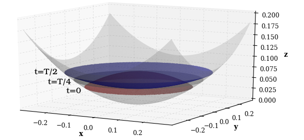
(a)	(b)

Figure 4: 3D Axisymmetrical parabolic bowl: (a) free surface at $t=0$ (red), $t=T/4$ (dark grey), $t=T/2$ (blue), with the period $T$ defined by $T=2\pi/\omega$, (b) velocity norm and vectors at $t=0,T/6,2T/6,T/2$, in $(x,y=0,z)$ slice plane.

In order to evaluate the convergence rate of the simulated solution $h_{sim}$ towards the analytical one $h_{anal}$, we plot the error rate versus the space discretization for five unstructured meshes with 1273 nodes and a single layer, 11104 nodes and 6 layers, 30441 nodes and 15 layers, 59473 nodes and 30 layers and 98137 nodes and 50 layers, see Remark 6.1. We have plotted (see Fig. 5) the $\mbox{log}(L^{2}-error)$ over the water depth at time $T=2\pi/\omega$ seconds versus $\mbox{log}(h_{a_{0}}/h_{a})$ for the first and second-order schemes and they are compared to the theoretical order.

Figure 5: Parabolic bowl: error between the analytical water depth and the simulated one with the five unstructured meshes. The curves for the first order scheme (space and time) and its second order extension (space and time) are compared to the first and second order theoretical curves (dashed lines).

Notice that on Fig. 5-(b), we have plotted the simulated solution obtained with 1 layer – that corresponds to the classical Saint-Venant system – and the simulated solution with 5 layers. The obtained convergence curves coincide proving the stability of the numerical scheme for the layers averaged system. The analytical solution is non stationary and hence, the errors due to the time scheme are combined with the one induced by the space discretization and it is the reason why we do not recover the theoretical order of convergence.

6.2.2 Draining of a tank

Considering the Navier-Stokes system (1)-(3) completed with the boundary conditions (5)-(8), the following proposition holds, see [40] for more details about the proposed analytical solution.

Proposition 6.2

For some $t_{0}\in\mathbb{R}$, $t_{1}\in\mathbb{R}_{+}^{*}$, $(\alpha,\beta)\in\mathbb{R}_{+}^{2}$ such that $\alpha\beta>L$, let us consider the functions $h,u,v,w,p,\phi$ defined for $t\geq t_{0}$ by

$$h(t,x,y)=\alpha f(t),$$

$$u(t,x,y,z)=\beta\left((z-z_{b})-\frac{\alpha}{2}f(t)\right)+f(t)(x\cos^{2}(\theta)+y\sin^{2}(\theta)),$$

$$v(t,x,y,z)=\beta\left((z-z_{b})-\frac{\alpha}{2}f(t)\right)+f(t)(x\cos^{2}(\theta)+y\sin^{2}(\theta)),$$

$$w(t,x,y,z)=f(t)(z_{b}-z),$$

$$p(t,x,y,z)=p^{a}(t,x,y)-2\nu f(t)+g(h-(z-z_{b})),$$

where $f(t)=1/(t-t_{0}+t_{1})$ and with a flat bottom $z_{b}(x,y)=z_{b,0}=cst$ and $p^{a}(t,x,y)=p^{a,1}(t)$, with $p^{a,1}(t)$ a given function.

Then $h,u,v,w,p$ as defined previously satisfy the 3d hydrostatic Navier-Stokes system (1)-(3) completed with the boundary conditions (6),(4),(7),(5) and $\kappa=\frac{2\nu\alpha\beta}{h(t,x,y)[\alpha\beta-2(x\cos^{2}(\theta)+y\sin^{2}(\theta))]}$ in (6), $W=\nu\beta/2$ with ${\bf t}_{s}=\frac{1}{\sqrt{2}}(1,1,0)^{t}$ in (7). The appropriate boundary conditions for $x\in\{-L/2,L/2\}$ or $y\in\{-L/2,L/2\}$ are also determined by the expressions of $h,v,u,w$ given above.

Choosing the viscosity $\nu=0$, the variables $h,u,v,w,p$ become analytical solutions of the 3d hydrostatic Euler system (12)-(13) completed with the boundary conditions (5),(4) and $p(t,x,y,\eta(t,x,y))=0$.

• The proof of prop. 6.2 relies on very simple computations and is not detailed here. $\blacksquare$

We have performed the simulations for several unstructured meshes of the geometrical domain $(x,y)\in[0,5]\times[0,1]$ and an adapted number of layers so that each 3d element of the mesh can be approximatively considered as a regular polyhedron, the considered meshes have 483 nodes and 3 layers, 700 nodes and 6 layers, 1306 nodes and 10 layers, 2781 nodes and 20 layers.

For $L=2$ m, $\alpha=1$ m.s, $t_{0}=0$ s, $t_{1}=0.5$ s, $\beta=2.5$ s^-1, $\theta=0$, $\nu=0$ m².s^-1, $p^{a,1}=0$ m².s^-2 on Fig. 6-(a), we have depicted the features of the analytical solution – at time $T=0.5$ second – we use for the convergence test. Figure 6-(b) gives the convergence curve towards the analytical solution i.e. the $\mbox{log}(L^{2}-error)$ of the water depth – at time $T=1$ second – versus $\mbox{log}(h_{a_{0}}/h_{a})$ for the first and second-order schemes and they are compared to the theoretical order (we denote by $h_{a}$ the average edge length and $h_{a_{0}}$ the average edge length of the coarser mesh). Notice that in this test case, the errors due to the space and time discretization are combined, this explains why the theoretical orders of convergence are not exactly obtained. Moreover, the boundary conditions (inflow prescribed) play an important role and since their numerical treatment is only at the first order in space, this also explains the difference between the theoretical and observed orders of convergence. With the mesh having 2781 nodes, we have tested the influence of the number of layers, see Fig. 6-(c). When the numbers of layers increase, we recover the analytical velocity profile.

(a)	(b)	(c)

Figure 6: Analytical solution given in prop. 6.2 : (a) slice of the fluid domain for $y=0.5$ m and velocity field at time $T=0.5\!$ s, (b) convergence curve towards the reference solution, first order (space and time) and second order extension (space and time) schemes. The first and second order theoretical curves correspond to the dashed lines. (c) Analytical horizontal velocity $u$ along $z$ at abscissa $x=L/2$ m and time $T$ and its simulated values for different numbers of layers.

6.3 Simulation of a tsunami

In this section, we test our discrete model in the case of a real tsunami propagation for which field measurements are available (free surface variations recorded by buoys). Even if in such cases, involving long wave propagation, 2d shallow water models can be used instead of 3d description, and we test here the capacity of our model and of the numerical procedure to handle this complex situation.

Simulation of tsunami waves generated by earthquakes is very important in Earth science for hazard assessment and for recovering earthquakes characteristics. Indeed, tsunami waves can be analyzed to recover the earthquake source that generated the tsunami and are now classically used in joint inversion methods. It has been shown that tsunami waves provide strong constraints on the spatial distribution of the source, especially in the case of shallow slip [42]. In some cases, far-field tsunami gauges may help constrain the earthquake source process even though they are affected by the compressibility of the water column and of the Earth [42, 43].

The 2014/04/01 Iquique earthquake struck off the coast of Chile at 20:46 local time (23:46 UTC), with a moment magnitude of 8.1. The epicenter of the earthquake was approximately 95 kilometers (59 mi) northwest of Iquique, as shown in Fig. 7.

We have carried out simulations of the tsunami induced by the earthquake using

• a topography obtained from the National Oceanic and Atmospheric Administration (NOAA, [44]) using the ETOPO1 data (1-arc minute global relief model),

• an unstructured mesh whose dimensions – a square of 2224.2 km² – correspond to the domain covered by Fig. 7,

• a source corresponding to the seafloor displacement induced by the earthquake (Fig. 7). This source is obtained by computing the 3D final displacements of the seafloor generated by the earthquake coseismic slip. This coseismic slip has been itself retrieved by inversion of numerous geodetic and seismic data, according to the model determined by [45]. The source is activated at time $t_{0}$, just after the earthquake occurrence ($t_{0}$ is here 2014/04/01,23h47mn25s)

We did not consider here the Coriolis force, the tides and the ocean currents. The results shown in Fig. 8 have been obtained with a mesh containing 545821 nodes and 5 layers (computation time was 35 minutes with a Mac book air 1.7 GHz Intel core i7). We compare the numerical solutions  – provided by the first order scheme (space and time) and the second order scheme (space and time) – with the DART measurements (obtained from the NOAA website http://www.ndbc.noaa.gov/dart.shtml). A series of simulations have been performed using several meshes and we present “converged” results in the sense that a finer mesh would give the same results. This is illustrated in Fig. 8-(d), where we plot the simulation results obtained with three meshes having respectively 311687 nodes (coarse mesh), 545821 nodes (fine mesh), and 985327 nodes (very fine mesh): the curves corresponding to the fine (cyan) and very fine (blue) curves are very similar.

Fig. 8-(a),(b),(c) shows that the second order scheme significantly improves the results both for the amplitude and phase of the water waves. The second order scheme is able to very accurately reproduce the shape of the first wave at the closest DART buoy 32401, located at 287 km from the epicenter. The two following peaks in the waveform are quite well reproduced up to about $1.755\times 10^{5}$ s. This is also the case at the DART buoy 32402, located 853 km from the epicenter. The arrival time of the first wave is very well reproduced at the three DART buoys, slightly better with the second order scheme. At the most distant buoy 32412 (1650 km from the source), the first order scheme is not able to reproduce the recorded wave. The second order scheme reproduces the first wave quite well but not the rest of the waveform, possibly due to Earth curvature effects that are not taken into account here. Globally, the low frequency content of the signals is better explained by the model than the high frequency fluctuations. These high frequency fluctuations may be related to effects not accounted for here, such as spatio-temporal heterogeneity of the real source, small wavelength fluctuation of the topography, and possibly non-hydrostatic effects [46, 47].

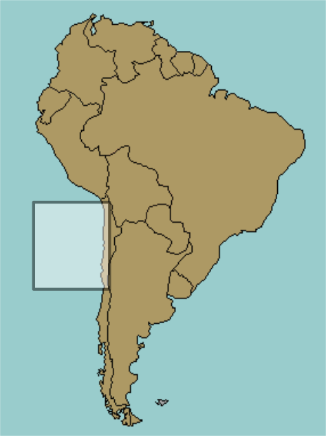
Figure 7: (Left) Location of the zone of interest, located offshore Northern Chile ; (Center) Bathymetric map showing the earthquake epicenter (red cone) and the location of the three DART buoys (black boxes); (Right) Vertical displacement (in centimeter) of the topography due to the earthquake. Horizontal displacements (not shown here) are also taken into account in the simulation.

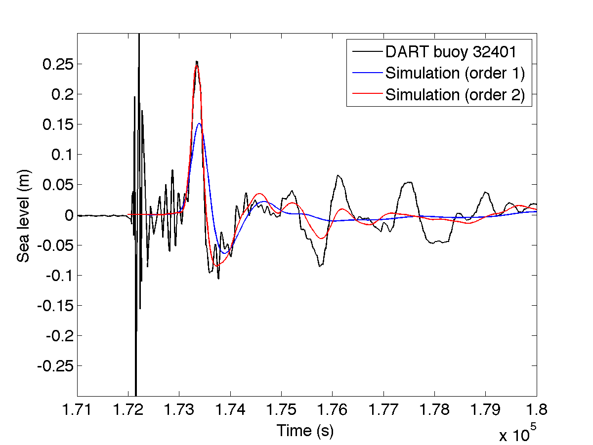
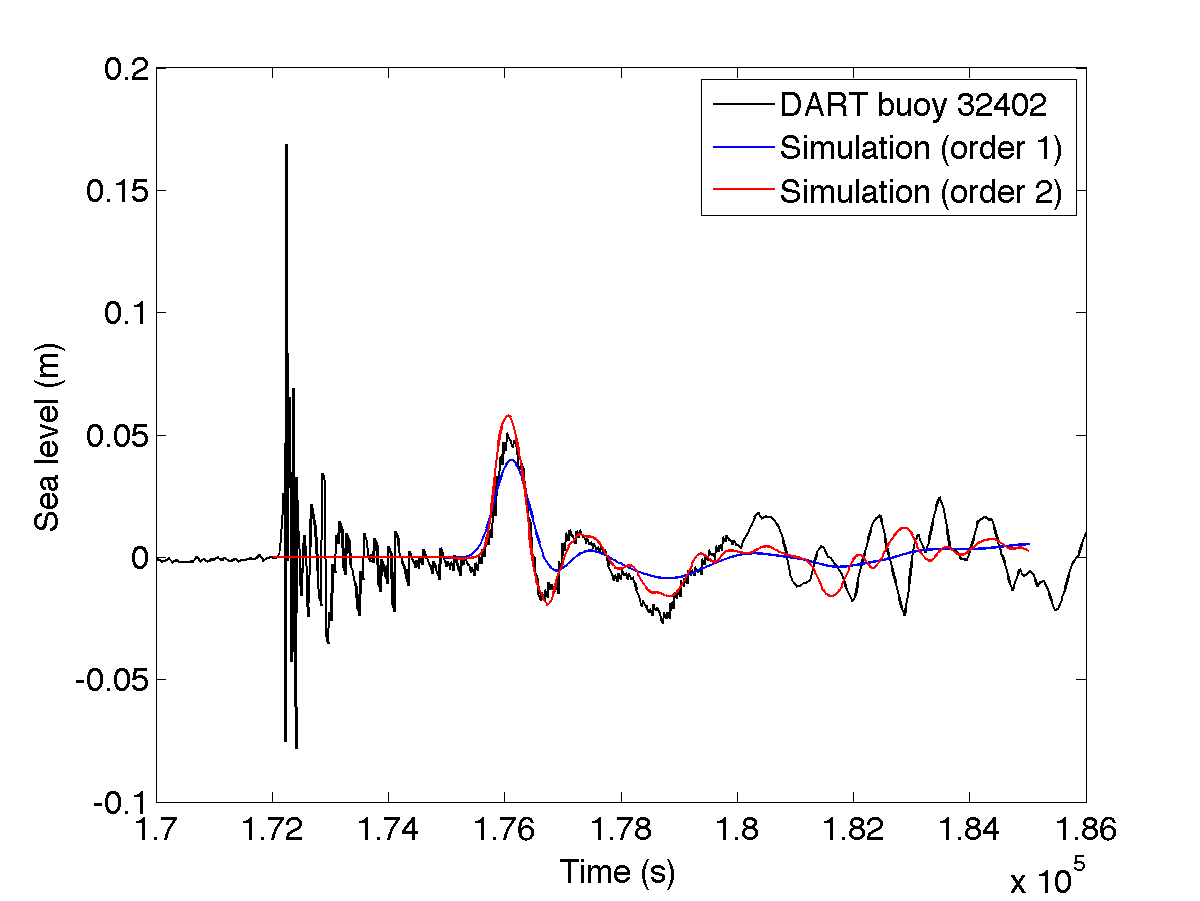
(a)	(b)
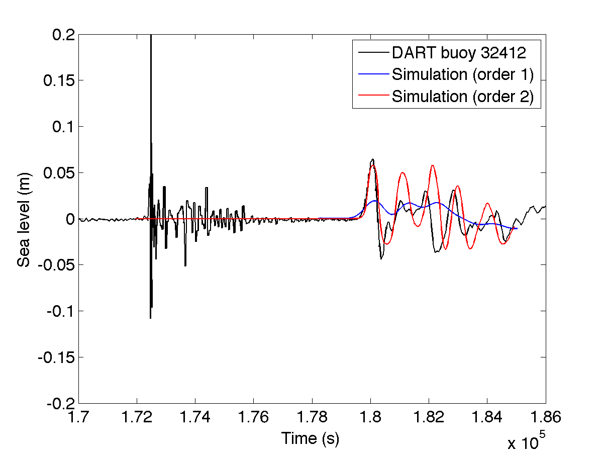
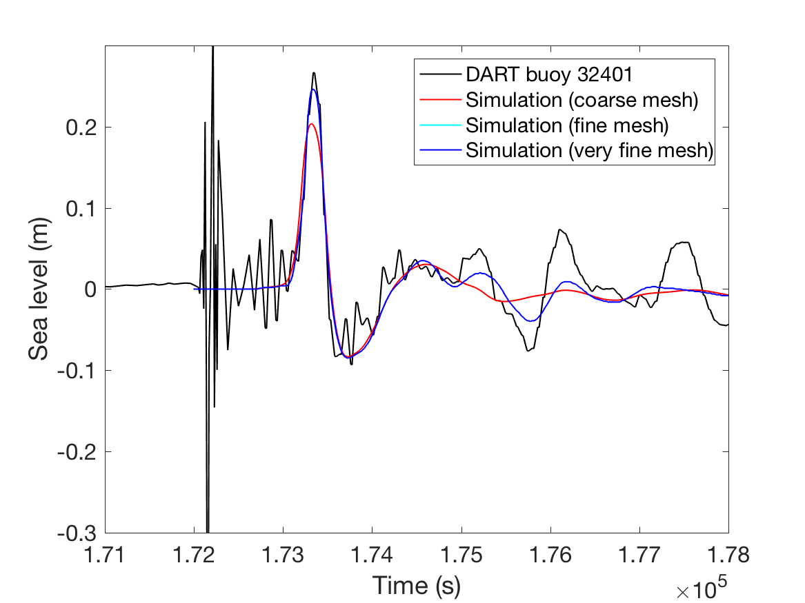
(c)	(d)

Figure 8: a), b) c) : Comparison between the sea level variations recorded by the 3 DART buoys and the corresponding simulations (1^st and 2^nd order schemes). d) Effect of the mesh size on the simulation accuracy for DART buoy 32401. In a), b), c), d), observations have been detided using a low pass Butterworth filter (order 4 and cutoff frequency of 4 hours), and the simulated waveforms have been filtered with the same Butterworth filter.

7 Conclusion

In this paper, we have presented a layer-averaged version of the 3d incompressible, hydrostatic Euler and Navier-Stokes systems with free surface. Based on a kinetic interpretation of the system for the Euler part, we have derived a stable, robust and efficient numerical scheme in a finite volume/finite element framework on unstructured meshes. The numerical scheme is endowed with strong stability properties (domain invariant, well-balancing, wet/dry interfaces treatment,…).

The numerical scheme is successfully validated with analytical solutions and is shown to be applicable to simulate complex test cases, like a tsunami propagation over a real bathymetry, proving its accuracy and efficiency.

Acknowledgements The authors thank Quentin Blétery for his involvement in the analysis of the 2014 Iquique earthquake (paragraph 6.3). We also thank Raphaël Grandin for its contribution in the computations of the bottom displacements necessary for the tsunami simulations. This work has been partially funded by the ERC Contract No. ERC-CG-2013-PE10-617472 SLIDEQUAKES. The authors also acknowledge the Inria Project Lab "Algae in Silico" for its financial support.

Appendix A

• Using the results of prop. 21, it remains to obtain the expression for the layer-averaged viscous terms.

  The layer-averaging of the viscous terms appearing in (2) gives

  $$\int_{z_{\alpha+1/2}}^{z_{\alpha+1/2}}\left(\frac{\partial\Sigma_{xx}}{\partial x}+\frac{\partial\Sigma_{xy}}{\partial y}+\nu\frac{\partial^{2}u}{\partial z^{2}}\right)dz = \frac{\partial}{\partial x}\left(h_{\alpha}\Sigma_{xx,\alpha}\right)+\frac{\partial}{\partial y}\left(h_{\alpha}\Sigma_{xy,_{\alpha}}\right)$$ (133)

  $$+\nu\left.\frac{\partial u}{\partial z}\right|_{\alpha+1/2}-\nu\left.\frac{\partial u}{\partial z}\right|_{\alpha-1/2}$$

  $$-\frac{\partial z_{\alpha+1/2}}{\partial x}\Sigma_{xx,\alpha+1/2}-\frac{\partial z_{\alpha+1/2}}{\partial y}\Sigma_{xy,\alpha+1/2}$$

  $$+\frac{\partial z_{\alpha-1/2}}{\partial x}\Sigma_{xx,\alpha-1/2}+\frac{\partial z_{\alpha-1/2}}{\partial y}\Sigma_{xy,\alpha-1/2},$$

  with

  $$h_{\alpha}\Sigma_{xx,\alpha} = \int_{z_{\alpha-1/2}}^{z_{\alpha-1/2}}\Sigma_{xx}dz.$$

  The boundary conditions at the bottom (6) and at the free surface (7) imply that in (133)

  $$\nu\left.\frac{\partial u}{\partial z}\right|_{N+1/2}-\frac{\partial\eta}{\partial x}\Sigma_{xx,N+1/2}-\frac{\partial\eta}{\partial y}\Sigma_{xy,N+1/2}=0,$$

  and

  $$\nu\left.\frac{\partial u}{\partial z}\right|_{1/2}-\frac{\partial z_{b}}{\partial x}\Sigma_{xx,1/2}-\frac{\partial z_{b}}{\partial y}\Sigma_{xy,1/2}=\kappa u_{1}.$$

  The above expression for $\Sigma_{xx,\alpha}$ and relation (133) have been obtained using the following formal computation

  $$\int_{z_{\alpha+1/2}}^{z_{\alpha+1/2}}\frac{\partial\Sigma_{xx}}{\partial x}dz = \frac{\partial}{\partial x}\int_{z_{\alpha+1/2}}^{z_{\alpha+1/2}}\Sigma_{xx}dz-\frac{\partial z_{\alpha+1/2}}{\partial x}\Sigma_{xx,\alpha+1/2}+\frac{\partial z_{\alpha-1/2}}{\partial x}\Sigma_{xx,\alpha-1/2}$$

  $$= \frac{\partial}{\partial x}\left(h_{\alpha}\Sigma_{xx,\alpha}\right)-\frac{\partial z_{\alpha+1/2}}{\partial x}\Sigma_{xx,\alpha+1/2}+\frac{\partial z_{\alpha-1/2}}{\partial x}\Sigma_{xx,\alpha-1/2}.$$

  The definitions (32),(33) are motivated by the following computation

  $$\frac{h_{\alpha+1}+h_{\alpha}}{2}\Sigma_{xx,\alpha+1/2} = \nu_{\alpha+1/2}\int_{z_{\alpha}}^{z_{\alpha+1}}\frac{\partial u}{\partial x}dz$$

  $$= \nu_{\alpha+1/2}\frac{\partial}{\partial x}\int_{z_{\alpha}}^{z_{\alpha+1}}udz-\nu_{\alpha+1/2}\frac{\partial z_{\alpha+1}}{\partial x}u_{\alpha+1}+\nu_{\alpha+1/2}\frac{\partial z_{\alpha}}{\partial x}u_{\alpha}$$

  $$= \nu_{\alpha+1/2}\frac{\partial}{\partial x}\left(\frac{h_{\alpha}}{2}u_{\alpha}+\frac{h_{\alpha+1}}{2}u_{\alpha+1}\right)-\nu_{\alpha+1/2}\frac{\partial z_{\alpha+1}}{\partial x}u_{\alpha+1}+\nu_{\alpha+1/2}\frac{\partial z_{\alpha}}{\partial x}u_{\alpha}$$

  $$= \nu_{\alpha+1/2}\left(\frac{h_{\alpha}}{2}\frac{\partial u_{\alpha}}{\partial x}+\frac{h_{\alpha+1}}{2}\frac{\partial u_{\alpha+1}}{\partial x}\right)-\nu_{\alpha+1/2}\frac{\partial z_{\alpha+1/2}}{\partial x}(u_{\alpha+1}-u_{\alpha}).$$

In order to prove the energy balance (36) we use the results of prop. 24 obtained for the layer-averaged Euler system and it remains to consider the viscous and frictions terms multiplied by ${\bf u}_{\alpha}$.

Let us define ${\bf R}_{\alpha}$

$${\bf R}_{\alpha}=\begin{pmatrix}R_{x,\alpha}\\ R_{y,\alpha}\end{pmatrix}=\nabla_{x,y}.\bigl{(}h_{\alpha}{\bf\Sigma}_{\alpha}\bigr{)}-{\bf\Sigma}_{\alpha+1/2}\nabla_{x,y}z_{\alpha+1/2}+{\bf\Sigma}_{\alpha-1/2}\nabla_{x,y}z_{\alpha-1/2}\\ +2\nu_{\alpha+1/2}\frac{{\bf u}_{{\alpha}+1}-{\bf u}_{\alpha}}{h_{{\alpha}+1}+h_{\alpha}}-2\nu_{\alpha-1/2}\frac{{\bf u}_{\alpha}-{\bf u}_{{\alpha}-1}}{h_{\alpha}+h_{{\alpha}-1}}-\kappa_{\alpha}{\bf u}_{\alpha}.$$

We write

$$R_{x,\alpha}u_{\alpha} = \frac{\partial\bigl{(}u_{\alpha}h_{\alpha}\Sigma_{xx,\alpha}\bigr{)}}{\partial x}+\frac{\partial\bigl{(}u_{\alpha}h_{\alpha}\Sigma_{xy,\alpha}\bigr{)}}{\partial y}$$

$$+\nu_{\alpha+1/2}\frac{u_{{\alpha}+1}+u_{\alpha}}{2}\frac{u_{{\alpha}+1}-u_{\alpha}}{h_{{\alpha}+1}+h_{\alpha}}-\nu_{\alpha-1/2}\frac{u_{\alpha}+u_{\alpha-1}}{2}\frac{u_{\alpha}-u_{\alpha-1}}{h_{\alpha}+h_{\alpha-1}}$$

$$-\frac{\partial z_{\alpha+1/2}}{\partial x}\Sigma_{xx,\alpha+1/2}u_{\alpha}-\frac{\partial z_{\alpha+1/2}}{\partial y}\Sigma_{xy,\alpha+1/2}u_{\alpha}$$

$$+\frac{\partial z_{\alpha-1/2}}{\partial x}\Sigma_{xx,\alpha-1/2}u_{\alpha}+\frac{\partial z_{\alpha-1/2}}{\partial y}\Sigma_{xy,\alpha-1/2}u_{\alpha}$$

$$-h_{\alpha}\Sigma_{xx,\alpha}\frac{\partial u_{\alpha}}{\partial x}-h_{\alpha}\Sigma_{xy,\alpha}\frac{\partial u_{\alpha}}{\partial y}$$

$$-\nu_{\alpha+1/2}\frac{(u_{\alpha+1}-u_{\alpha})^{2}}{h_{{\alpha}+1}+h_{\alpha}}-\nu_{\alpha-1/2}\frac{(u_{\alpha}-u_{\alpha-1})^{2}}{h_{\alpha}+h_{{\alpha}-1}}-\kappa_{\alpha}u^{2}_{\alpha},$$

and using the closure relation (34), it comes for $\alpha=2,\ldots,N-1$

$$R_{x,\alpha}u_{\alpha} = \frac{\partial\bigl{(}u_{\alpha}h_{\alpha}\Sigma_{xx,\alpha}\bigr{)}}{\partial x}+\frac{\partial\bigl{(}u_{\alpha}h_{\alpha}\Sigma_{xy,\alpha}\bigr{)}}{\partial y}$$

$$+\nu_{\alpha+1/2}\frac{u_{{\alpha}+1}+u_{\alpha}}{2}\frac{u_{{\alpha}+1}-u_{\alpha}}{h_{{\alpha}+1}+h_{\alpha}}-\nu_{\alpha+1/2}\frac{u_{\alpha}+u_{\alpha-1}}{2}\frac{u_{\alpha}-u_{\alpha-1}}{h_{\alpha}+h_{\alpha-1}}$$

$$-\Sigma_{xx,\alpha+1/2}\left(\frac{h_{\alpha}}{2}\frac{\partial u_{\alpha}}{\partial x}+\frac{\partial z_{\alpha+1/2}}{\partial x}u_{\alpha}\right)-\Sigma_{xy,\alpha+1/2}\left(\frac{h_{\alpha}}{2}\frac{\partial u_{\alpha}}{\partial y}+\frac{\partial z_{\alpha+1/2}}{\partial y}u_{\alpha}\right)$$

$$+\Sigma_{xx,\alpha-1/2}\left(-\frac{h_{\alpha}}{2}\frac{\partial u_{\alpha}}{\partial x}+\frac{\partial z_{\alpha-1/2}}{\partial x}\frac{u_{\alpha}}{2}\right)+\Sigma_{xy,\alpha-1/2}\left(-\frac{h_{\alpha}}{2}\frac{\partial u_{\alpha}}{\partial y}+\frac{\partial z_{\alpha-1/2}}{\partial y}\frac{u_{\alpha}}{2}\right)$$

$$-\nu_{\alpha+1/2}\frac{(u_{\alpha+1}-u_{\alpha})^{2}}{h_{{\alpha}+1}+h_{\alpha}}-\nu_{\alpha-1/2}\frac{(u_{\alpha}-u_{\alpha-1})^{2}}{h_{\alpha}+h_{{\alpha}-1}}-\kappa_{\alpha}u^{2}_{\alpha}.$$

An analogous relation can be easily obtained for $R_{y,\alpha}v_{\alpha}$ and computing the sum over the layers of the obtained quantity, we get

$$\sum_{\alpha=1}^{N}{\bf R}_{\alpha}.{\bf u}_{\alpha} = \sum_{\alpha=1}^{N}\left(\frac{\partial\bigl{(}u_{\alpha}h_{\alpha}\Sigma_{xx,\alpha}\bigr{)}}{\partial x}+\frac{\partial\bigl{(}u_{\alpha}h_{\alpha}\Sigma_{xy,\alpha}\bigr{)}}{\partial y}+\frac{\partial\bigl{(}v_{\alpha}h_{\alpha}\Sigma_{yx,\alpha}\bigr{)}}{\partial x}+\frac{\partial\bigl{(}v_{\alpha}h_{\alpha}\Sigma_{yy,\alpha}\bigr{)}}{\partial y}\right)$$

$$-\sum_{\alpha=1}^{N-1}\frac{h_{\alpha+1}+h_{\alpha}}{2\nu}\left(\Sigma_{xx,\alpha+1/2}^{2}+\Sigma_{xy,\alpha+1/2}^{2}+\Sigma_{yx,\alpha+1/2}^{2}+\Sigma_{yy,\alpha+1/2}^{2}\right)$$

$$-\sum_{\alpha=1}^{N-1}2\nu\frac{|{\bf u}_{{\alpha}+1}-{\bf u}_{\alpha}|^{2}}{h_{{\alpha}+1}+h_{\alpha}}-\kappa|{\bf u}_{1}|^{2},$$

proving the result. $\blacksquare$

Appendix B

Simple computations give

$$F_{h} = h\int_{\{y_{1}\geq-\frac{\tilde{u}}{c}\}\times\mathbb{R}}(\tilde{u}+cy_{1})\chi_{0}(y_{1},y_{2})dy_{1}dy_{2}$$ (134)

$$= h\int_{y_{1}=-\frac{\tilde{u}}{c}}^{+\infty}(\tilde{u}+cy_{1})\left(\int_{-\infty}^{+\infty}\chi_{0}(y_{1},y_{2})dy_{2}\right)dy_{1}=\frac{h}{\pi}\int_{y_{1}=-\frac{\tilde{u}}{c}}^{+\infty}(\tilde{u}+cy_{1})\sqrt{1-\frac{y_{1}^{2}}{4}}dy_{1},$$

$$F_{hu} = h\int_{\{y_{1}\geq-\frac{\tilde{u}}{c}\}\times\mathbb{R}}(\tilde{u}+cy_{1})(u+cn_{x}y_{1})\chi_{0}(y_{1},y_{2})dy_{1}dy_{2}$$

$$= \frac{h}{\pi}\int_{y_{1}=-\frac{\tilde{u}}{c}}^{+\infty}(\tilde{u}+cy_{1})(u+cn_{x}y_{1})\sqrt{1-\frac{y_{1}^{2}}{4}}dy_{1},$$

and likewise for $F_{hv}$ we have

$$\begin{split}F_{hv}&=\frac{h}{\pi}\int_{y_{1}=-\frac{\tilde{u}}{c}}^{+\infty}(\tilde{u}+cy_{1})(v+cn_{y}y_{1})\sqrt{1-\frac{y_{1}^{2}}{4}}dy_{1}.\end{split}$$

It is possible to obtain explicit formula for the expressions of $F_{h}$, $F_{hu}$ and $F_{hv}$ since defining

$$\begin{split}&I_{1}(z)=\int^{z}(u+cz)\sqrt{1-\frac{z^{2}}{4}}dz,\qquad I_{2}(z)=\int^{z}(u+cz)(v+cnz)\sqrt{1-\frac{z^{2}}{4}}dz,\end{split}$$

we have

$$I_{1}(z)=-\frac{4c}{3}\left(1-\frac{z^{2}}{4}\right)^{3/2}+u\left(\frac{z}{2}\sqrt{1-\frac{z^{2}}{4}}+\arcsin\left(\frac{z}{2}\right)\right),$$

and

$$I_{2}(z)=-c^{2}nz\left(1-\frac{z^{2}}{4}\right)^{3/2}+\frac{c^{2}n+uv}{2}z\sqrt{1-\frac{z^{2}}{4}}\\ +(c^{2}n+uv)\arcsin\left(\frac{z}{2}\right)-\frac{4c(nu+v)}{3}\left(1-\frac{z^{2}}{4}\right)^{3/2}.$$

Therefore, it comes

$$\begin{split}F_{h}&=\left\{\begin{array}[]{ll}0&\mbox{if }-\frac{\tilde{u}}{c}\geq 2\\ \frac{h}{\pi}\tilde{u}\arcsin(\frac{\tilde{u}}{2c})+\frac{h\tilde{u}}{2}+\frac{h}{c}\left(\frac{\tilde{u}^{2}}{6}+\frac{4}{3}c^{2}\right)\chi_{0}\left(\frac{\tilde{u}}{c}\right)&\mbox{if }-2\leq-\frac{\tilde{u}}{c}\leq 2\\ h&\mbox{if }-\frac{\tilde{u}}{c}\leq-2\end{array}\right.\\ F_{hu}&=\left\{\begin{array}[]{ll}0&\mbox{if }-\frac{\tilde{u}}{c}\geq 2\\ \frac{h}{\pi}(c^{2}n_{x}+u\tilde{u})\arcsin\left(\frac{\tilde{u}}{2c}\right)+\frac{h}{2}(c^{2}n_{x}+u\tilde{u})&\\ \quad+\frac{h}{12c}\left(2u\tilde{u}^{2}-n_{x}\tilde{u}^{3}+16c^{2}u+10c^{2}\tilde{u}n_{x}\right)\chi_{0}\left(\frac{\tilde{u}}{c}\right)&\mbox{if }-2\leq-\frac{\tilde{u}}{c}\leq 2\\ hu\tilde{u}+hc^{2}n_{x}&\mbox{if }-\frac{\tilde{u}}{c}\leq-2\end{array}\right.\\ F_{hv}&=\left\{\begin{array}[]{ll}0&\mbox{if }-\frac{\tilde{u}}{c}\geq 2\\ \frac{h}{\pi}(c^{2}n_{y}+v\tilde{u})\arcsin\left(\frac{\tilde{u}}{2c}\right)+\frac{h}{2}(c^{2}n_{y}+v\tilde{u})&\\ \quad+\frac{h}{12c}\left(2v\tilde{u}^{2}-n_{y}\tilde{u}^{3}+16c^{2}v+10c^{2}\tilde{u}n_{y}\right)\chi_{0}\left(\frac{\tilde{u}}{c}\right)&\mbox{if }-2\leq-\frac{\tilde{u}}{c}\leq 2\\ hv\tilde{u}+hc^{2}n_{y}&\mbox{if }-\frac{\tilde{u}}{c}\leq-2\end{array}\right.\\ \end{split}$$

References

- [1] Barré de Saint-Venant AJC. Théorie du mouvement non permanent des eaux avec applications aux crues des rivières et à l’introduction des marées dans leur lit. C R Acad Sci Paris. 1871;73:147–154.
- [2] Bouchut F, Westdickenberg M. Gravity driven shallow water models for arbitrary topography. Comm in Math Sci. 2004;2:359–389.
- [3] Perthame B. Kinetic formulation of conservation laws. Oxford University Press; 2002.
- [4] Audusse E, Bouchut F, Bristeau MO, Sainte-Marie J. Kinetic entropy inequality and hydrostatic reconstruction scheme for the Saint-Venant system. Math Comp. 2016;85(302):2815–2837. Available from: http://dx.doi.org/10.1090/mcom/3099.
- [5] Audusse E. A multilayer Saint-Venant model : Derivation and numerical validation. Discrete Contin Dyn Syst Ser B. 2005;5(2):189–214.
- [6] Audusse E, Bristeau MO. Finite-volume solvers for a multilayer Saint-Venant system. Int J Appl Math Comput Sci. 2007;17(3):311–319.
- [7] Audusse E, Bristeau MO, Decoene A. Numerical simulations of 3d free surface flows by a multilayer Saint-Venant model. Internat J Numer Methods Fluids. 2008;56(3):331–350.
- [8] Bouchut F, Morales de Luna T. An entropy satisfying scheme for two-layer shallow water equations with uncoupled treatment. M2AN Math Model Numer Anal. 2008;42:683–698.
- [9] Castro MJ, García-Rodríguez JA, González-Vida JM, Macías J, Parés C, Vázquez-Cendón ME. Numerical simulation of two-layer shallow water flows through channels with irregular geometry. J Comput Phys. 2004;195(1):202–235.
- [10] Castro MJ, Macías J, Parés C. A Q-SCHEME FOR A CLASS OF SYSTEMS OF COUPLED CONSERVATION LAWS WITH SOURCE TERM. APPLICATION TO A TWO-LAYER 1-D SHALLOW WATER SYSTEM. M2AN Math Model Numer Anal. 2001;35(1):107–127.
- [11] Ovsyannikov LV. Two-layer shallow water models. Prikl Mekh Tekh Fiz. 1979;2:3–14.
- [12] Vreugdenhil CB. Two-layer Shallow-Water Flow in Two Dimensions, a Numerical Study. J Comput Phys. 1979;33:169–184.
- [13] Bouchut F, Zeitlin V. A robust well-balanced scheme for multi-layer shallow water equations. Discrete Contin Dyn Syst Ser B. 2010;13:739–758.
- [14] Fernández-Nieto ED, Koné EH, Chacón Rebollo T. A multilayer method for the hydrostatic Navier-Stokes equations: a particular weak solution. Journal of Scientific Computing. 2014;60(2):408–437. Available from: http://dx.doi.org/10.1007/s10915-013-9802-0.
- [15] Audusse E, Bristeau MO, Perthame B, Sainte-Marie J. A multilayer Saint-Venant system with mass exchanges for Shallow Water flows. Derivation and numerical validation. ESAIM: M2AN. 2011;45:169–200. Available from: http://dx.doi.org/10.1051/m2an/2010036.
- [16] Audusse E, Bristeau MO, Pelanti M, Sainte-Marie J. Approximation of the hydrostatic Navier-Stokes system for density stratified flows by a multilayer model. Kinetic interpretation and numerical validation. J Comp Phys. 2011;230:3453–3478.
- [17] Sainte-Marie J. Vertically averaged models for the free surface Euler system. Derivation and kinetic interpretation. Math Models Methods Appl Sci (M3AS). 2011;21(3):459–490.
- [18] Bristeau MO, Di-Martino B, Guichard C, Sainte-Marie J. Layer-averaged Euler and Navier-Stokes equations. Commun Math Sci. 2017 Jun;15(5):1221–1246. Available from: https://hal.inria.fr/hal-01202042.
- [19] Fernández-Nieto ED, Garres-Dìas G, Mangeney A, Narbona-Reina G. A multilayer shallow model for dry granular flows with the (I)-rheology: Application to granular collapse on erodible beds. Journal of Fluid Mechanics. 2016;.
- [20] Casulli V. A semi-implicit numerical method for the free-surface Navier-Stokes equations. Internat J Numer Methods Fluids. 2014;74(8):605–622. Available from: http://dx.doi.org/10.1002/fld.3867.
- [21] Hervouet JM. Hydrodynamics of Free Surface Flows: Modelling with the Finite Element Method. Wiley; 2007.
- [22] Audusse E, Bristeau MO, Sainte-Marie J. Kinetic entropy for layer-averaged hydrostatic Navier-Stokes equations; 2017. submitted.
- [23] Freshkiss3d home page; 2017. http://freshkiss3d.gforge.inria.fr.
- [24] Lions PL. Mathematical Topics in Fluid Mechanics. Vol. 1: Incompressible models. Oxford University Press; 1996.
- [25] Brenier Y. Homogeneous hydrostatic flows with convex velocity profiles. Nonlinearity. 1999;12(3):495–512.
- [26] Grenier E. On the derivation of homogeneous hydrostatic equations. ESAIM: M2AN. 1999;33(5):965–970.
- [27] Masmoudi N, Wong T. On the Hs Theory of Hydrostatic Euler Equations. Archive for Rational Mechanics and Analysis. 2012;204(1):231–271. Available from: http://dx.doi.org/10.1007/s00205-011-0485-0.
- [28] Bresch D, Kazhikhov A, Lemoine J. On the two-dimensional hydrostatic Navier-Stokes equations. SIAM J Math Anal. 2004/05;36(3):796–814. Available from: https://doi.org/10.1137/S0036141003422242.
- [29] Perthame B, Simeoni C. A kinetic scheme for the Saint-Venant system with a source term. Calcolo. 2001;38(4):201–231.
- [30] Bouchut F. Construction of BGK models with a family of kinetic entropies for a given system of conservation laws. J Stat Phys. 1999;95:113–170.
- [31] Bouchut F. Entropy satisfying flux vector splittings and kinetic BGK models. Numer Math. 2003;94:623–672.
- [32] Berthelin F, Bouchut F. Relaxation to isentropic gas dynamics for a BGK system with single kinetic entropy. Methods Appl Anal. 2002;9(2):313–327. Available from: http://dx.doi.org/10.4310/MAA.2002.v9.n2.a7.
- [33] Audusse E, Bristeau MO. A well-balanced positivity preserving second-order scheme for Shallow Water flows on unstructured meshes. J Comput Phys. 2005;206(1):311–333.
- [34] Bouchut F. Nonlinear stability of finite volume methods for hyperbolic conservation laws and well-balanced schemes for sources. Birkhäuser; 2004.
- [35] Audusse E, Bouchut F, Bristeau MO, Klein R, Perthame B. A Fast and Stable Well-Balanced Scheme with Hydrostatic Reconstruction for Shallow Water Flows. SIAM J Sci Comput. 2004;25(6):2050–2065.
- [36] Bristeau MO, Coussin B. Boundary Conditions for the Shallow Water Equations solved by Kinetic Schemes. INRIA; 2001. RR-4282. Available from: http://hal.inria.fr/inria-00072305/en/.
- [37] Van Leer B. Towards the ultimate conservative difference scheme. V. A second-order sequel to Godunov’s method. J Comput Phys. 1997;135(2):227–248. With an introduction by Ch. Hirsch, Commemoration of the 30th anniversary {of J. Comput. Phys.}. Available from: http://dx.doi.org/10.1006/jcph.1997.5757.
- [38] Bouchut F. An introduction to finite volume methods for hyperbolic conservation laws. ESAIM Proc. 2004;15:107–127.
- [39] Boulanger AC, Sainte-Marie J. Analytical solutions for the free surface hydrostatic Euler equations. Commun Math Sci. 2013;11(4):993–1010.
- [40] Bristeau MO, DI Martino B, Mangeney A, Sainte-Marie J, Souillé F. Various analytical solutions for the incompressible Euler and Navier-Stokes systems with free surface; 2018. Working paper or preprint. Available from: https://hal.archives-ouvertes.fr/hal-01831622.
- [41] Thacker WC. Some exact solutions to the non-linear shallow-water wave equations. J Fluid Mech. 1981;107:499–508.
- [42] Gusman A, Murotani S, Satake K, Heidarzadeh M, Gunawan E, Watada S, et al. Fault slip distribution of the 2014 Iquique, Chile, earthquake estimated from ocean-wide tsunami waveforms and GPS data. Geophysical Research Letters. 2015;42(4):1053–1060. 2014GL062604. Available from: http://dx.doi.org/10.1002/2014GL062604.
- [43] Watada S, Kusumoto S, Satake K. Traveltime delay and initial phase reversal of distant tsunamis coupled with the self-gravitating elastic Earth. Journal of Geophysical Research: Solid Earth. 2014;119(5):4287–4310. 2013JB010841. Available from: http://dx.doi.org/10.1002/2013JB010841.
- [44] NOAA home page; 2017. https://www.ngdc.noaa.gov/mgg/global/global.html.
- [45] Vallée M, Grandin R, Ruiz S, Delouis B, Vigny C, Rivera E, et al. Complex rupture of an apparently simple asperity during the 2014/04/01 Pisagua earthquake (Northern Chile, Mw=8.1). In: EGU General Assembly Conference Abstracts. vol. 18, EGU2016-8660; 2016. .
- [46] Bristeau MO, Mangeney A, Sainte-Marie J, Seguin N. An energy-consistent depth-averaged Euler system: Derivation and properties. Discrete and Continuous Dynamical Systems - Series B. 2015;20(4):961–988. Available from: http://aimsciences.org/journals/displayArticlesnew.jsp?paperID=10801.
- [47] As̈siouene N, Bristeau MO, Godlewski E, Sainte-Marie J. A robust and stable numerical scheme for a depth-averaged Euler system - https://hal.inria.fr/hal-01162109; 2015. Available from: https://hal.inria.fr/hal-01162109.