A Fast Algorithm Based on a Sylvester-like Equation for LS Regression with GMRF Prior

Abstract

This paper presents a fast approach for penalized least squares (LS) regression problems using a 2D Gaussian Markov random field (GMRF) prior. More precisely, the computation of the proximity operator of the LS criterion regularized by different GMRF potentials is formulated as solving a Sylvester-like matrix equation. By exploiting the structural properties of GMRFs, this matrix equation is solved column-wise in an analytical way. The proposed algorithm can be embedded into a wide range of proximal algorithms to solve LS regression problems including a convex penalty. Experiments carried out in the case of a constrained LS regression problem arising in a multichannel image processing application, provide evidence that an alternating direction method of multipliers performs quite efficiently in this context.

I Introduction

Constrained or penalized least squares (LS) problems have been widely encountered in various signal/image processing applications, such as spectral unmixing [1, 2, 3], supervised source separation [4], image classification [5], material quantification [6] or subpixel detection [7]. The LS problem often results from the following linear model which has been successfully used in the applications mentioned above:

$$\bf Y=WH+N$$ (1)

where ${\mathbf{Y}}\in\mathbb{R}^{m\times n}$ is the observed data matrix (each row of ${\mathbf{Y}}$ is the vectorized version of an image), ${\mathbf{W}}\in\mathbb{R}^{m\times d}$ is a basis matrix that will be assumed to be known in this work, ${\mathbf{H}}\in\mathbb{R}^{d\times n}$ is a matrix containing the regression coefficients, and ${\mathbf{N}}\in\mathbb{R}^{m\times n}$ is the noise term which can be assumed to follow a multivariate Gaussian distribution. Note that LS can be classically interpreted as projecting the observed data onto the subspace spanned by the columns of ${\mathbf{W}}$.

As the LS problem associated with (1) is usually ill-posed, e.g., some columns of ${\mathbf{W}}$ may be similar, it is necessary to introduce priors/regularizations for ${\mathbf{H}}$ to make the problem well-conditioned [8]. Enforcing spatial regularization on the matrix ${\mathbf{H}}$ is a strategy for incorporating prior information, e.g., total variation (TV), Markov random field (MRF) penalty, sparsity constraints in the wavelet domain, etc. Among these, a powerful and important way of exploiting the correlations between pixels of an image is to consider Gaussian Markov random fields (GMRFs), which have been extensively used in image processing applications such as denoising [9], super-resolution [10], segmentation [11] and spectral unmixing [12]. Constructing a GMRF amounts to define a finite-dimensional random vector with a multivariate normal distribution having nontrivial conditional Markov dependence properties. GMRFs allow us to exploit analytical results obtained for the Gaussian distribution and to enforce Markovian properties, leading to computationally efficient algorithms. In general, different images can be characterized by GMRF distributions with different parameters. For example, the distributions of water and soil in a remote sensing image can be modeled by two different GMRF distributions based upon their physical locations. Mathematically, the GMRF regularizations associated with the two rows of ${\mathbf{H}}$ corresponding to water and soil should obviously be different. This diversity makes the corresponding optimization problem quite challenging, leading to the solution of a tensor equation. A number of efficient sampling algorithms such as those based on Markov chain Monte Carlo (MCMC) algorithms have been designed for statistical inference, which are effective but generally time consuming [13, 12].

In this paper, we adopt a proximal approach [14] to address this variational problem. We start by showing that the computation of the proximity operator of the LS criterion with GMRF regularization can be performed by solving a Sylvester-like matrix equation and propose an algorithm to solve it analytically by taking advantage of the properties of stationary 2D GMRFs. More specifically, the block circulant properties of the covariance matrix of such a field is exploited to simplify the associated matrix equation. The resulting closed-form solution is easy to implement and very fast to compute.

This paper is organized as follows. Section II formulates the regularized LS regression for the considered class of linear models and GMRF priors. Section III addresses the problem of computing the associated proximity operator by solving in a fast manner a Sylvester-like matrix equation. Section IV shows the benefit of this approach for solving more challenging convex optimization problems. Simulation results are presented in Section V showing the good performance of the proposed approach, whereas conclusions are reported in Section VI.

II Problem formulation

II-A Observation model

Decomposing the matrices ${\mathbf{W}}$ and ${\mathbf{H}}$ as ${\mathbf{W}}=[{\mathbf{w}}_{1},\cdots,{\mathbf{w}}_{d}]$ and ${\mathbf{H}}^{T}=[{\mathbf{h}}_{1},\cdots,{\mathbf{h}}_{d}]$, where ${\mathbf{w}}_{k}$ is the $k$th column of ${\mathbf{W}}$ and ${\mathbf{h}}_{i}^{T}$ is the $i$th row of ${\mathbf{H}}$, (1) can be rewritten as

$${\mathbf{Y}}=\sum_{i=1}^{d}{\mathbf{w}}_{i}{\mathbf{h}}_{i}^{T}+{\mathbf{N}}.$$ (2)

Note that each pixel (column) of the image (matrix) ${\mathbf{Y}}$ is the linear combination of $d$ basis vectors ${\mathbf{w}}_{1},\cdots,{\mathbf{w}}_{d}$ (e.g., $d$ materials whose signatures are the columns of ${\mathbf{W}}$). Estimating the matrix ${\mathbf{H}}$ from the observed matrix ${\mathbf{Y}}$ with possible constraints about the vectors ${\mathbf{h}}_{i}$ is a classical LS problem that has been considered in particular in source separation [15] and spectral unmixing [1, 16].

II-B Gaussian Markov Random Fields

According to the Hammersley-Clifford theorem [17, 13], an MRF can equivalently be characterized by a Gibbs distribution. More specifically, a zero-mean Gaussian random field $(h_{k})_{1\leq k\leq n}\in\mathbb{R}$ satisfying

$$p(h_{k}\mid{h_{\ell},\ell\neq k})=p(h_{k}\mid{h_{\ell},\ell\in{\mathcal{N}}_{k}})$$ (3)

where ${\mathcal{N}}_{k}$ contains the neighbors of the $k$th element $h_{k}$, is a GMRF. The distribution of ${\mathbf{h}}=[h_{1},\cdots,h_{k}]^{T}$ can be written as

$$p({\mathbf{h}})=\frac{1}{c}\exp{\left(-\frac{\lambda}{2}\sum_{k=1}^{n}\big{(}h_{k}-\sum_{\ell\in{\mathcal{N}}_{k}}\alpha_{\ell}h_{\ell}\big{)}^{2}\right)}$$ (4)

where $\lambda>0$ is a scale parameter and the normalizing constant $c>0$ is the partition function of this probability distribution, which is generally unknown. Equivalently, (4) reads

$$p({\mathbf{h}})=\frac{1}{c}\exp{\left(-\frac{\lambda}{2}\|{\mathbf{h}}-{\mathbf{Q}}{\mathbf{h}}\|_{2}^{2}\right)}$$ (5)

where $\lambda({\mathbf{I}}-{\mathbf{Q}})^{T}({\mathbf{I}}-{\mathbf{Q}})$ is the precision matrix, ${\mathbf{I}}$ denotes the identity matrix and, in the 2D stationary case with periodic boundary condition, ${\mathbf{Q}}$ is a block circulant matrix with circulant blocks (BCCB) with its first column built from the coefficient vector $\boldsymbol{\alpha}=\left(\alpha_{1},\ldots,\alpha_{q}\right)^{T}$, $q=|{\mathcal{N}}_{k}|$ being the number of elements in the neighborhood of $h_{k}$.

III Fast computation of the proximity operator of the least squares criterion with GMRF prior

Assuming that the columns of ${\mathbf{H}}$ are independent and assigned a GMRF prior and considering the likelihood term from (1) leads to the following LS regression problem:

$$\underset{\begin{subarray}{c}{{\mathbf{H}}\in\mathbb{R}^{d\times n}}\end{subarray}}{\text{\rm minimize}}\;\;f({\mathbf{H}})$$ (6)

where

$$f({\mathbf{H}})=\frac{1}{2}\|{\mathbf{Y}}-\sum_{i=1}^{d}{\mathbf{w}}_{i}{\mathbf{h}}_{i}^{T}\|_{\rm F}^{2}+\sum_{i=1}^{d}\frac{\lambda_{i}}{2}\|{\mathbf{h}}_{i}^{T}-{\mathbf{h}}_{i}^{T}{\mathbf{Q}}_{i}\|^{2}.$$

Hereabove, $\|\cdot\|_{\rm F}$ denotes the Frobenius norm, and for every $i\in\{1,\ldots,d\}$, $\lambda_{i}$ is a positive parameter and ${\mathbf{Q}}_{i}$ is a BCCB matrix constructed from the MRF coefficients associated with the $i$th row of ${\mathbf{H}}$. Thus, ${\mathbf{Q}}_{i}$ enforces possible different spatial structures to ${\mathbf{h}}_{1},\cdots,{\mathbf{h}}_{d}$. Note that, because of its form, ${\mathbf{Q}}_{i}$ can be diagonalized in the frequency domain, i.e., ${\mathbf{Q}}_{i}={\mathbf{F}}{\mathbf{D}}_{i}{\mathbf{F}}^{H}$, where ${\mathbf{F}}$ is the 2D FFT matrix and ${\mathbf{F}}^{H}$ is its inverse.

In the following, we will be interested in the following more general optimization problem:

$$\underset{\begin{subarray}{c}{{\mathbf{H}}\in\mathbb{R}^{d\times n}}\end{subarray}}{\text{\rm minimize}}\;\;f({\mathbf{H}})+\frac{\gamma}{2}\|{\mathbf{H}}-\overline{{\mathbf{H}}}\|^{2}_{\rm F}$$ (7)

where $\gamma\geq 0$ and the second term means that ${\mathbf{H}}$ is close to $\overline{{\mathbf{H}}}$. When $\gamma=0$, this problem reduces to solving (6) and, when $\gamma>0$, this problem corresponds to the computation of $\text{\rm prox}_{\gamma^{-1}f}$, the proximity operator of $\gamma^{-1}f$ [18]. As we will see in the next section, such a proximity operator constitutes a key tool for solving optimization problems more involved than (6). Since $f$ is a quadratic function, it is well-know that $\text{\rm prox}_{\gamma^{-1}f}$ is a linear operator for which a closed-form expression can be obtained [14]. We show next that, rather than applying the direct formula (see [14, Table 10.1xi]), a more efficient approach can be adopted to compute this proximity operator.

Forcing the derivative of the objective function in (7) w.r.t. each ${\mathbf{h}}_{j}$ to be zero and substituting ${\mathbf{Q}}_{j}={\mathbf{F}}{\mathbf{D}}_{j}{\mathbf{F}}^{H}$ in the resulting equation leads to

$${\mathbf{w}}_{j}^{T}\left({\mathbf{W}}{\mathbf{H}}-{\mathbf{Y}}\right)+\lambda_{j}{\mathbf{h}}_{j}^{T}{\mathbf{F}}({\mathbf{I}}-{\mathbf{D}}_{j})^{2}{\mathbf{F}}^{H}+\gamma({\mathbf{h}}_{j}-\overline{{\mathbf{h}}}_{j})^{T}=\bf 0$$ (8)

for every $j\in\{1,\ldots,d\}$. Note that the matrix $\lambda_{j}({\mathbf{I}}-{\mathbf{D}}_{j})^{2}$ is a real diagonal matrix whose vector of diagonal elements is denoted by ${\mathbf{m}}_{j}$. Thus, (8) can be rewritten as

$$\begin{split}&{\mathbf{w}}_{j}^{T}\left({\mathbf{W}}{\mathbf{H}}-{\mathbf{Y}}\right){\mathbf{F}}+({\mathbf{h}}_{j}^{T}{\mathbf{F}})\odot{\mathbf{m}}_{j}^{T}+\gamma({\mathbf{h}}_{j}-\overline{{\mathbf{h}}}_{j})^{T}{\mathbf{F}}=\bf 0\end{split}$$ (9)

where $\odot$ is the Hadamard (element-wise) product. Stacking these $d$ equations leads to the following matrix equation

$$({\mathbf{W}}^{T}{\mathbf{W}}+\gamma{\mathbf{I}}){\mathbf{H}}{\mathbf{F}}+({\mathbf{H}}{\mathbf{F}})\odot{\mathbf{M}}=({\mathbf{W}}^{T}{\mathbf{Y}}+\gamma\overline{{\mathbf{H}}}){\mathbf{F}}.$$ (10)

Note that the matrix ${\mathbf{M}}$ can be decomposed as ${\mathbf{M}}=[{\boldsymbol{m}}_{1},\cdots,{\boldsymbol{m}}_{n}]$ $=[{\mathbf{m}}_{1},\cdots,{\mathbf{m}}_{d}]^{T}$, where a bold italic notation is used to designate the column of ${\mathbf{M}}$ while a bold non-italic one designates its rows. Eq. (10) is a Sylvester-like matrix equation[19, 20, 21, 22] w.r.t. $\widetilde{{\mathbf{H}}}=\bf HF$. Let $\widetilde{{\mathbf{h}}}_{k}$ be the $k$th column of the matrix $\widetilde{{\mathbf{H}}}$ and let $[({\mathbf{W}}^{T}{\mathbf{Y}}+\gamma\overline{{\mathbf{H}}}){\mathbf{F}}]_{k}$ be the $k$th column of $({\mathbf{W}}^{T}{\mathbf{Y}}+\gamma\overline{{\mathbf{H}}}){\mathbf{F}}$. Decomposing (10) column-wise allows the estimation of the different vectors $(\widetilde{{\mathbf{h}}}_{k})_{1\leq k\leq n}$ to be decoupled:

$$\widetilde{{\mathbf{h}}}_{k}=\left({\mathbf{W}}^{T}{\mathbf{W}}+\gamma{\mathbf{I}}+\textrm{diag}({\boldsymbol{m}}_{k})\right)^{-1}[({\mathbf{W}}^{T}{\mathbf{Y}}+\gamma\overline{{\mathbf{H}}}){\mathbf{F}}]_{k}$$ (11)

for every $k\in\{1,\cdots,n\}$, where $\textrm{diag}({\boldsymbol{m}}_{k})$ is the diagonal matrix whose diagonal is filled with the components of ${\boldsymbol{m}}_{k}$. The solution to Problem (7) is finally given by

$${\mathbf{H}}=\widetilde{{\mathbf{H}}}{\mathbf{F}}^{H}.$$ (12)

If $\max\{d,m\}\ll n$, the computational complexity of the previous strategy is of the order ${\mathcal{O}}(3dn\log_{2}n)$ because of the low cost of the 2D-FFT operation. The whole procedure to compute $\text{\rm prox}_{\gamma^{-1}f}(\overline{{\mathbf{H}}})$ is summarized in Algorithm 1.

Input: ${\mathbf{Y}}$, ${\mathbf{W}}$, $({\mathbf{Q}}_{i})_{1\leq i\leq d}$, $\overline{{\mathbf{H}}}$, $\boldsymbol{\lambda}=(\lambda_{i})_{1\leq i\leq d}$, $\gamma$

// 2D Fourier diagonalisation of $({\mathbf{Q}}_{i})_{1\leq i\leq d}$

1 for $i=1$ to $d$ do

       ${\mathbf{D}}_{i}\leftarrow{\mathbf{F}}^{H}{\mathbf{Q}}_{i}{\mathbf{F}}$; // one 2D-FFT required

2       ${\mathbf{m}}_{i}=\lambda_{i}\textrm{diag}\big{(}({\mathbf{I}}-{\mathbf{D}}_{i})^{2}\big{)}$;

3      

4 end for

// Compute the FFT of ${\mathbf{H}}$ for all pixels in parallel

5 for $k=1$ to $n$ do

6       Compute $\widetilde{{\mathbf{h}}}_{k}$ using (11);

7 end for

$\hat{{\mathbf{H}}}\leftarrow\bar{{\mathbf{H}}}{\mathbf{F}}^{H}$ Output: $\hat{{\mathbf{H}}}$

Algorithm 1 Computation of the proximity operator of the LS criterion with GMRF prior

IV Penalized LS with a GMRF prior

Having a fast way of computing the proximity operator of the LS criterion with GMRF prior yields efficient solutions to the following broad class of variational formulations:

$$\underset{\begin{subarray}{c}{{\mathbf{H}}\in\mathbb{R}^{d\times n}}\end{subarray}}{\text{\rm minimize}}\;\;\frac{1}{2}\|{\mathbf{Y}}-{\mathbf{W}}{\mathbf{H}}\|_{\rm F}^{2}+\sum_{i=1}^{d}\frac{\lambda_{i}}{2}\|{\mathbf{h}}_{i}^{T}-{\mathbf{h}}_{i}^{T}{\mathbf{Q}}_{i}\|^{2}+g({\mathbf{H}})$$ (13)

where $g\colon\mathbb{R}^{d\times n}\to]-\infty,+\infty]$ is an additional regularization term, here assumed to be a convex, lower-semicontinuous and proper function. For example, if ${\mathbf{H}}$ is known to belong to a nonempty closed convex set ${\mathcal{C}}\subset\mathbb{R}^{d\times n}$, a constrained least squares (CLS) regression is obtained by setting $g$ equal to the indicator function of ${\mathcal{C}}$, i.e.

$$(\forall{\mathbf{U}}\in\mathbb{R}^{d\times n})\quad g({\mathbf{U}})=\iota_{{\mathcal{C}}}({\mathbf{U}})=\left\{\begin{array}[]{ll}0&\textrm{if }{\mathbf{U}}\in{\mathcal{C}}\\ +\infty&\textrm{otherwise.}\end{array}\right.$$ (14)

Looking for a solution to (13) amounts to finding a minimizer of $f+g$. Provided that the proximity operator of $g$ is easy to compute, a wide range of proximal algorithms can be employed [14, 24] having good convergence properties. In particular, if $g$ is given by (14), this operator reduces to the projection $\Pi_{{\mathcal{C}}}$ onto ${\mathcal{C}}$.

As an example of proximal approaches which can be used, Algorithm 2 describes the iterative steps to be followed in order to implement the alternating direction of multipliers method (ADMM) [25, 26].

Input: ${\mathbf{Y}}$, ${\mathbf{W}}$, $({\mathbf{Q}}_{i})_{1\leq i\leq d}$, ${\mathbf{U}}^{(0)}$, ${\mathbf{G}}^{(0)}$, $\boldsymbol{\lambda}$, $\gamma$

// Initialize ${\mathbf{U}}$ and ${\mathbf{G}}$ with ${\mathbf{U}}^{(0)}$ and ${\mathbf{G}}^{(0)}$

1 $\hat{{\mathbf{U}}}\leftarrow{\mathbf{U}}^{(0)}$;

2 $\hat{{\mathbf{G}}}\leftarrow{\mathbf{G}}^{(0)}$;

// ADMM iterations

3 repeat

4       Update $\hat{{\mathbf{H}}}$: $\hat{{\mathbf{H}}}\leftarrow\text{\rm prox}_{\gamma^{-1}f}(\hat{{\mathbf{U}}}+\hat{{\mathbf{G}}})$

5       by feeding Algorithm 1 with

6       (${\mathbf{Y}}$, ${\mathbf{W}}$, $({\mathbf{Q}}_{i})_{1\leq i\leq d}$, $\hat{{\mathbf{U}}}+\hat{{\mathbf{G}}}$, $\boldsymbol{\lambda}$, $\gamma$);

7       Update $\hat{{\mathbf{U}}}$: $\hat{{\mathbf{U}}}\leftarrow\text{\rm prox}_{\gamma^{-1}g}(\hat{{\mathbf{H}}}-\hat{{\mathbf{G}}})$;

8       Update $\hat{{\mathbf{G}}}$: $\hat{{\mathbf{G}}}\leftarrow\hat{{\mathbf{G}}}-\hat{{\mathbf{H}}}+\hat{{\mathbf{U}}}$;

9until convergence;

Output: $\hat{{\mathbf{H}}}$

Algorithm 2 Penalized LS with GMRF regularization

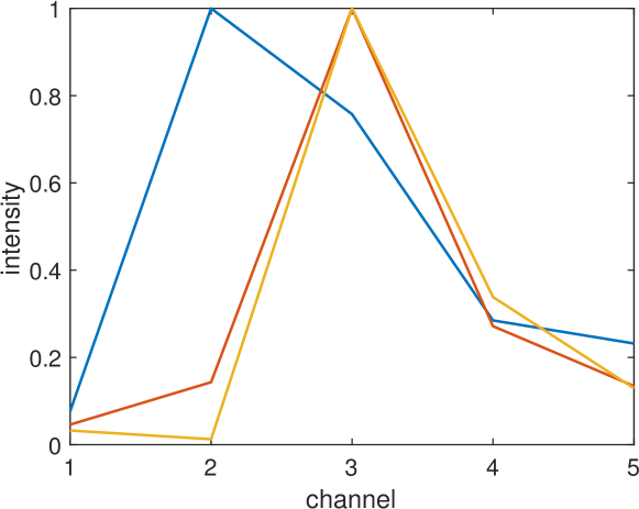
Figure 1: Columns of the matrix ${\mathbf{W}}$.

V Experiments

This section evaluates the performance of our algorithm for a multichannel image processing problem, and compares it with two widely used optimization algorithms: forward backward (FB) [27] and FISTA [28]. For a fair comparison, all the algorithms have been implemented using MATLAB R2016b on an HP EliteBook Folio 9470m with Intel(R) Core(TM) i7-3687U CPU @2.10GHz and 16GB RAM.

V-A Simulation scenario

In all the experiments, we consider a matrix ${\mathbf{W}}\in\mathbb{R}^{5\times 3}$ corresponding to measurements acquired in five channels and decomposed in a basis defined by three vectors. The three columns of the basis matrix ${\mathbf{W}}$ are displayed in Fig. 1. These vectors represent the signatures of three different fluorescent protein spectra [29]. One can note that two of them (red and brown) are quite similar, which makes the model very ill-posed. The matrix ${\mathbf{H}}$ has been generated row by row after vectorizing $3$ texture images available at http://sipi.usc.edu/database/. The three images we have considered in this work are displayed in the first row of Fig. 4 showing clear oriented structures. The GMRF parameters for these three images have been estimated using the maximum likelihood method [30] and are summarized in Fig. 2. Note that these GMRFs consider $3\times 3$ neighbors around one pixel and that half of them are set to zeros due to the symmetry property. The size of the images is $512\times 512$. In our simulations, the regularization parameters $(\lambda_{i})_{1\leq i\leq 3}$ for all bands are chosen equal to $0.05$ empirically (in real application this value vary depending on the noise power). The convex penalty function $g$ is the indicator of the box constraint ${\mathbf{H}}\in[0,1]^{d\times n}$.

The observed data are finally generated using the linear mixing model (1), i.e., $\bf Y=WH+N$, where the noise matrix ${\mathbf{N}}$ has been generated using samples of a Gaussian distribution with zero mean and covariance matrix $\sigma^{2}{\mathbf{I}}$. The variance $\sigma^{2}$ has been adjusted in order to have an initial SNR (signal to noise ratio) equal to $25$dB.

$$\begin{bmatrix}-0.26&0.55&0\\ 0.13&0&0\\ 0.58&0&0\\ \end{bmatrix}\begin{bmatrix}-0.19&0.78&0\\ 0.35&0&0\\ 0.042&0&0\\ \end{bmatrix}\begin{bmatrix}-0.68&0.79&0\\ 0.84&0&0\\ 0.047&0&0\\ \end{bmatrix}$$

Figure 2: Estimated GMRF coefficients for ${\mathbf{h}}_{1}$, ${\mathbf{h}}_{2}$ and ${\mathbf{h}}_{3}$ (left to right).

V-B Quality Assessment

To analyze the quality of the proposed estimation method, we have considered the normalized mean square error (NMSE) defined as

$$\textrm{NMSE}=\frac{\|\hat{{\mathbf{H}}}-{\mathbf{H}}\|^{2}_{\rm F}}{\|{\mathbf{H}}\|^{2}_{\rm F}}.$$

The smaller NMSE, the better the estimation quality.

V-C Comparison with existing optimization algorithms

The evolution of the relative error between the iterates and the solution to (13) versus execution time, is displayed in Fig. 3(left) for the three tested algorithms, namely FB, FISTA and the proposed one. Here, the optimal solution $\mathbf{H}^{*}$ has been precomputed for each algorithm using a large number of iterations. We also show the NMSE versus time in Fig. 3(right). All the algorithms lead to the same estimation quality as expected. However, as demonstrated in these plots, the proposed algorithm based on a Sylvester-like equation solver is faster than FB and FISTA. More precisely, the proposed algorithm converges rapidly in a few steps while the other two need more iterations and time to converge. One can also note that FISTA converges faster than FB, both in terms of error on the iterates and NMSE decays.

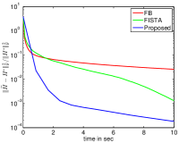
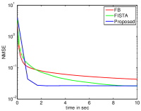
Figure 3: Convergence comparison of different algorithms: (left) relative distance to the solution vs time, (right) NMSE vs time.

To demonstrate the role of the GMRF regularization, we computed the box constrained (${\mathbf{H}}\in[0,1]^{d\times n}$) LS regression without any regularization, by setting $\lambda_{i}=0$ for every $i\in\{1,2,3\}$ and use it as a baseline for comparison. The regression matrix ${\mathbf{H}}$ estimated by LS and by the proposed approach are displayed in the second and third rows of Fig. 4, respectively. Due to the ill-posedness of the problem, the inversion without any spatial regularization amplifies the noise, leading to poor estimation results as shown in the second row of Fig. 4 (especially for the second and third images). The GMRF model plays a very important role in restoring satisfactorily the spatial structures and details as shown in the last row of Fig. 4. The NMSE values indicated in the caption of Fig. 4 corroborate these visual comparisons.

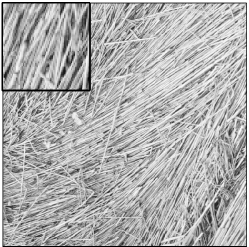
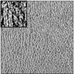
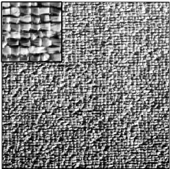
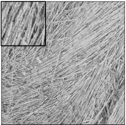
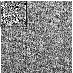
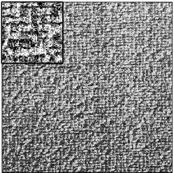
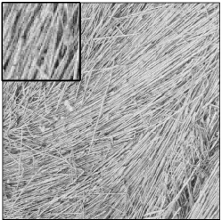
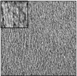
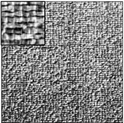
Figure 4: Regression matrix ${\mathbf{H}}$ and its estimates $\hat{{\mathbf{H}}}$ for texture images ($512\times 512$): (top) ground-truth, (middle) LS estimator (NMSE = $0.166$), (bottom) LS estimator with GMRF (NMSE = $0.026$). A zoom of each image is displayed in its left top side.

VI Conclusion

This paper developed a new algorithm for penalized least squares regression with GMRF regularization based on a Sylvester-like matrix equation solver. The closed-form solution of this equation makes it very appealing in terms of computational complexity. Although we have focused on the use of ADMM, the proposed approach can be embedded into most of the existing proximal methods to solve penalized or constrained least squares regression problems. Numerical experiments confirmed the effectiveness of the resulting algorithms. Future work includes the generalization of the proposed algorithm to applications where the basis matrix is partially known or unknown.

References

- [1] N. Keshava and J. F. Mustard, “Spectral unmixing,” IEEE Signal Process. Mag., vol. 19, no. 1, pp. 44–57, Jan. 2002.
- [2] E. Chouzenoux, M. Legendre, S. Moussaoui, and J. Idier, “Fast constrained least squares spectral unmixing using primal-dual interior-point optimization,” IEEE J. Sel. Topics Appl. Earth Observ. Remote Sens., vol. 7, no. 1, pp. 59–69, 2014.
- [3] Q. Wei, J. Bioucas-Dias, N. Dobigeon, and J.-Y. Tourneret, “Fast spectral unmixing based on Dykstra’s alternating projection,” Univ. of Toulouse, IRIT/INP-ENSEEIHT, Tech. Rep., 2015. [Online]. Available: http://arxiv.org/abs/1505.01740
- [4] N. Dobigeon, S. Moussaoui, M. Coulon, J.-Y. Tourneret, and A. O. Hero, “Joint Bayesian endmember extraction and linear unmixing for hyperspectral imagery,” IEEE Trans. Signal Process., vol. 57, no. 11, pp. 4355–4368, 2009.
- [5] C.-I Chang, X.-L. Zhao, M. L. G. Althouse, and J. J. Pan, “Least squares subspace projection approach to mixed pixel classification for hyperspectral images,” IEEE Trans. Geosci. Remote Sens., vol. 36, no. 3, pp. 898–912, May 1998.
- [6] J. Wang and C.-I Chang, “Applications of independent component analysis in endmember extraction and abundance quantification for hyperspectral imagery,” IEEE Trans. Geosci. Remote Sens., vol. 4, no. 9, pp. 2601–2616, Sept. 2006.
- [7] D. Manolakis, C. Siracusa, and G. Shaw, “Hyperspectral subpixel target detection using the linear mixing model,” IEEE Trans. Geosci. Remote Sens., vol. 39, no. 7, pp. 1392–1409, July 2001.
- [8] C. L. Lawson and R. J. Hanson, Solving least squares problems. Englewood Cliffs, NJ: Prentice-hall, 1974, vol. 161.
- [9] M. Malfait and D. Roose, “Wavelet-based image denoising using a Markov random field a priori model,” IEEE Trans. Image Process., vol. 6, no. 4, pp. 549–565, Apr. 1997.
- [10] T. Kasetkasem, M. K. Arora, and P. K. Varshney, “Super-resolution land cover mapping using a Markov random field based approach,” Remote Sens. Environment, vol. 96, no. 3, pp. 302–314, 2005.
- [11] C. D’Elia, G. Poggi, and G. Scarpa, “A tree-structured Markov random field model for Bayesian image segmentation,” IEEE Trans. Image Process., vol. 12, no. 10, pp. 1259–1273, Oct. 2003.
- [12] O. Eches, J. A. Benediktsson, N. Dobigeon, and J.-Y. Tourneret, “Adaptive Markov random fields for joint unmixing and segmentation of hyperspectral images,” IEEE Trans. Image Process., vol. 22, no. 1, pp. 5–16, Jan. 2013.
- [13] H. Rue and L. Held, Gaussian Markov Random Fields: Theory and Applications. Florida, USA: CRC Press, 2005.
- [14] P. L. Combettes and J.-C. Pesquet, “Proximal splitting methods in signal processing,” in Fixed-Point Algorithms for Inverse Problems in Science and Engineering, ser. Springer Optimization and Its Applications, H. H. Bauschke, R. S. Burachik, P. L. Combettes, V. Elser, D. R. Luke, and H. Wolkowicz, Eds. Springer New York, 2011, pp. 185–212.
- [15] M. Zibulevsky and B. A. Pearlmutter, “Blind source separation by sparse decomposition in a signal dictionary,” Neural computation, vol. 13, no. 4, pp. 863–882, 2001.
- [16] D. C. Heinz and C.-I. Chang, “Fully constrained least squares linear spectral mixture analysis method for material quantification in hyperspectral imagery,” IEEE Trans. Geosci. Remote Sens., vol. 39, no. 3, pp. 529–545, 2001.
- [17] P. Clifford, “Markov random fields in statistics,” Disorder in physical systems: A volume in honour of John M. Hammersley, pp. 19–32, 1990.
- [18] H. H. Bauschke and P. L. Combettes, Convex Analysis and Monotone Operator Theory in Hilbert Spaces. New York: Springer, 2011.
- [19] Q. Wei, N. Dobigeon, and J.-Y. Tourneret, “Fast fusion of multi-band images based on solving a Sylvester equation,” IEEE Trans. Image Process., vol. 24, no. 11, pp. 4109–4121, Nov. 2015.
- [20] ——, “FUSE: A fast multi-band image fusion algorithm,” in Proc. IEEE Int. Workshop Comput. Adv. Multi-Sensor Adaptive Process. (CAMSAP), Cancun, Mexico, Dec. 2015, pp. 161–164.
- [21] N. Zhao, Q. Wei, A. Basarab, N. Dobigeon, D. Kouamé, and J. Y. Tourneret, “Fast single image super-resolution using a new analytical solution for problems,” IEEE Trans. Image Process., vol. 25, no. 8, pp. 3683–3697, Aug. 2016.
- [22] N. Zhao, Q. Wei, A. Basarab, D. Kouamé, and J. Y. Tourneret, “Single image super-resolution of medical ultrasound images using a fast algorithm,” in Proc. IEEE Int. Symp. Biomed. Imaging (ISBI). Prague, Czech Republic: IEEE, Apr. 2016, pp. 473–476.
- [23] R. H. Bartels and G. Stewart, “Solution of the matrix equation AX+ XB= C [F4],” Communications of the ACM, vol. 15, no. 9, pp. 820–826, 1972.
- [24] N. Komodakis and J.-C. Pesquet, “Playing with duality: An overview of recent primal-dual approaches for solving large-scale optimization problems.” IEEE Signal Process. Mag., vol. 32, no. 6, pp. 31–54, Nov. 2015.
- [25] J. M. Bioucas-Dias and M. A. Figueiredo, “Alternating direction algorithms for constrained sparse regression: Application to hyperspectral unmixing,” in Proc. IEEE GRSS Workshop Hyperspectral Image SIgnal Process.: Evolution in Remote Sens. (WHISPERS), Reykjavik, Iceland, Jun. 2010, pp. 1–4.
- [26] S. Boyd, N. Parikh, E. Chu, B. Peleato, and J. Eckstein, “Distributed optimization and statistical learning via the alternating direction method of multipliers,” Foundations and Trends in Machine Learning, vol. 3, no. 1, pp. 1–122, 2011.
- [27] P. L. Combettes and V. R. Wajs, “Signal recovery by proximal forward-backward splitting,” Multiscale Modeling & Simulation, vol. 4, no. 4, pp. 1168–1200, 2005.
- [28] A. Beck and M. Teboulle, “A fast iterative shrinkage-thresholding algorithm for linear inverse problems,” SIAM J. Imaging Sci., vol. 2, no. 1, pp. 183–202, 2009.
- [29] C. Ricard and F. Debarbieux, “Six-color intravital two-photon imaging of brain tumors and their dynamic microenvironment,” Front Cell Neurosci., pp. 8–57, Feb. 2014.
- [30] C. S. Won and H. Derin, “Maximum likelihood estimation of Gaussian Markov random field parameters,” in Proc. IEEE Int. Conf. Acoust., Speech, and Signal Processing (ICASSP), vol. 2, New York, USA, Apr. 1988, pp. 1040–1043.