Fragmentation of Filamentary Cloud Permeated by Perpendicular Magnetic Field

Abstract

We examine the linear stability of an isothermal filamentary cloud permeated by a perpendicular magnetic field. Our model cloud is assumed to be supported by gas pressure against the self-gravity in the unperturbed state. For simplicity, the density distribution is assumed to be symmetric around the axis. Also for simplicity, the initial magnetic field is assumed to be uniform and turbulence is not taken into account. The perturbation equation is formulated to be an eigenvalue problem. The growth rate is obtained as a function of the wavenumber for fragmentation along the axis and the magnetic field strength. The growth rate depends critically on the outer boundary. If the displacement vanishes in the region very far from the cloud axis (fixed boundary), cloud fragmentation is suppressed by a moderate magnetic field, which means the plasma beta is below 1.67 on the cloud axis. If the displacement is constant along the magnetic field in the region very far from the cloud, the cloud is unstable even when the magnetic field is infinitely strong. The cloud is deformed by circulation in the plane perpendicular to the magnetic field. The unstable mode is not likely to induce dynamical collapse, since it is excited even when the whole cloud is magnetically subcritical. For both the boundary conditions the magnetic field increases the wavelength of the most unstable mode. We find that the magnetic force suppresses compression perpendicular to the magnetic field especially in the region of low density.

=3

1 INTRODUCTION

It is widely accepted that stars form from the fragmentation of filamentary clouds (see, e.g., André et al., 2014, and the references therein). This idea is supported by observations showing that the filamentary structure is universal in interstellar clouds and that prestellar cores and newly formed stars are associated with the dense parts of filamentary clouds. It is also well known that filamentary clouds are unstable against fragmentation if they are gravitationally bound (see, e.g., Stodólkiewicz, 1963; Larson, 2003, and the references therein).

Fragmentation of a magnetized filamentary cloud has been studied extensively (see, e.g., Stodólkiewicz, 1963; Nakamura, Hanawa & Nakano, 1993; Hanawa et al., 1993; Fiege & Pudritz, 2000), particularly in 1990s. We note that the magnetic field was generally assumed to be either parallel or helical to the cloud axis in these studies. However, fragmentation depends on the magnetic field direction, since the magnetic force is perpendicular to the local magnetic field. We know that massive main filamentary clouds are often associated with a magnetic field perpendicular to the axis, although less massive sub-filaments are parallel to the magnetic field (see, e.g., Sugitani et al., 2011; Palmeirim et al., 2013; André et al., 2014; Kusune et al., 2016, and the references therein). Prestellar cores are often associated with the main filaments. Thus, we should examine the effects of the magnetic field perpendicular to the cloud axis on fragmentation.

It is not easy to construct a self-consistent model of a filamentary molecular cloud associated with a magnetic field perpendicular to the cloud axis. Consequently, it is not easy to analyze the stability against fragmentation. As shown in Tomisaka (2014), the cloud is likely to be flattened, like fettuccine pasta. His equilibrium model shows that the cloud is supported in part by the magnetic force against gravity. The numerically obtained density distribution is difficult to apply in a stability analysis. Hanawa & Tomisaka (2015) examined fragmentation of a filamentary cloud permeated by a perpendicular magnetic field under the approximation that the filamentary cloud is highly flattened in the direction perpendicular to the magnetic field. They neglected the density structure along the magnetic field.

With the abovementioned difficulties in mind, we examine the stability of a simple self-consistent model for a magnetized filamentary cloud. The model cloud is assumed to be isothermal and supported against the self-gravity solely by the gas pressure in equilibrium. The initial magnetic field is assumed to be uniform and perpendicular to the cloud axis so that the magnetic force vanishes in the initial state. Although turbulence is dominant over the thermal pressure, especially in the low density region, we ignore interstellar turbulence for simplicity. Nevertheless, some effects of turbulence may be taken into account effectively by replacing the sound speed with the typical turbulent velocity. The model cloud is also assumed to be infinitely long and the density to be a function of the radius from the axis. The magnetic field works against fragmentation through tension. We evaluate the effects of the magnetic field on fragmentation by conducting a linear stability analysis. The growth rate of the instability is obtained as a function of the wavelength and the magnetic field strength, i.e., the initial plasma beta at the cloud center.

This paper is organized as follows. We describe our equilibrium model and methods of stability analysis in §2. We employ two types of boundary conditions, fixed and free, for the magnetic field in the region very far from the cloud center. The result of the stability analysis is presented in §3. The growth rate is shown to depend on the choice of boundary condition. We discuss the implication of our stability analysis in §4. In Appendix A, we prove that an unstable mode has a real growth rate. In Appendix B, we describe the elements of the matrixes used for our stability analysis. In Appendix C, we calculate the growth rate for an unmagnetized filamentary cloud in order to evaluate the accuracy of our numerical analysis.

2 METHODS

2.1 Basic Equations

For our stability analysis, we employ the ideal magnetohydrodymamic (MHD) equations,

$$\frac{\partial\rho}{\partial t}+\mbox{\boldmath$\nabla$}\cdot\left(\rho\mbox{\boldmath$v$}\right)=0,$$ (1)

$$\rho\frac{d\mbox{\boldmath$v$}}{dt}=-\mbox{\boldmath$\nabla$}P+\mbox{\boldmath$j$}\times\mbox{\boldmath$B$}+\rho\mbox{\boldmath$\nabla$}\Phi,$$ (2)

$$\mbox{\boldmath$j$}=\frac{\mbox{\boldmath$\nabla$}\times\mbox{\boldmath$B$}}{4\pi},$$ (3)

where $\rho$, $P$, $\Phi$ , $v$, $B$ $,and$ $j$ denote the density, pressure, gravitational potential, velocity, magnetic field, and electric current density, respectively. The gas is assumed to be isothermal and so the equation of state is expressed as

$$P = \rho c_{s}^{2},$$ (4)

where $c_{s}$ denotes the sound speed. The self-gravity of the gas is taken into account through the Poisson equation

$$\Delta\Phi=4\pi G\rho,$$ (5)

where $G$ denotes the gravitational constant. We ignore ambipolar diffusion and turbulence for simplicity.

2.2 Equilibrium Model

We consider an isothermal filamentary cloud in hydrostatic equilibrium. The cloud axis is assumed to be located on $x=y=0$ in Cartesian coordinates. Then the density distribution is expressed as

$$\rho_{0}(x,y,z) = \rho_{c}\left(1+\frac{x^{2}+y^{2}}{8H^{2}}\right)^{-2},$$ (6)

$$H^{2} = \frac{c_{s}^{2}}{4\pi G\rho_{c}},$$ (7)

where $\rho_{0}$ and $\rho_{c}$ denote the density distribution in equilibrium and the value on the cloud axis, respectively (Stodólkiewicz, 1963; Ostriker, 1964).

We assume that the cloud in equilibrium is permeated by a uniform magnetic field in the $x$-direction,

$$\mbox{\boldmath{$B$}}_{0}=B_{0}\mbox{\boldmath$e$}_{x},$$ (8)

where $\mbox{\boldmath$e$}_{x}$ denotes the unit vector in the $x$-direction. This uniform magnetic field does affect the cloud stability but not the equilibrium.

To specify the initial magnetic field strength in the analysis, we use the plasma beta at the cloud center,

$$\beta = \frac{8\pi\rho_{c}c_{s}^{2}}{B_{0}^{2}}.$$ (9)

The plasma beta is related to the mass to flux ratio,

$$f = \frac{\displaystyle\int\rho_{0}(x^{\prime},y,z)dx^{\prime}}{B_{0}}$$ (10)

$$= \frac{\sqrt{2}\pi\rho_{c}H}{B_{0}}\left(1+\frac{y^{2}}{8H^{2}}\right)^{-3/2}.$$ (11)

The mass to flux ratio can be rewritten as

$$f = \frac{1}{4}\sqrt{\displaystyle\frac{\beta}{G}}\left(1+\frac{y^{2}}{8H^{2}}\right)^{-3/2},$$ (12)

by using Equation (7). The critical mass to flux ratio is $f_{c}=1/(2\pi\sqrt{G})$. Thus, the cloud is subcritical when

$$\beta < 0.405\left(1+\frac{y^{2}}{8H^{2}}\right)^{3}.$$ (13)

2.3 Perturbation Equation

We consider a small perturbation around the equilibrium in order to search for an unstable mode. The perturbation is described by the displacement defined by

$$\xi = \xi_{x}(x,y)\cos kz\mbox{\boldmath${e}$}_{x}+\xi_{y}(x,y)\cos kz\mbox{\boldmath$e$}_{y}$$ (14)

$$+\xi_{z}(x,y)\sin kz\mbox{\boldmath$e$}_{z},$$

where the perturbation is assumed to be sinusoidal in the $z$-direction with the wavenumber $k$. The density perturbation is derived from the equation of continuity,

$$\delta\rho=-\mbox{\boldmath$\nabla$}\cdot\left(\rho_{0}\mbox{\boldmath$\xi$}\right).$$ (15)

Substituting Equation (14) into Equation (15), we obtain

$$\delta\rho(x,y,z) = \delta\varrho(x,y)\cos kz,$$ (16)

$$\delta\varrho = -\frac{\partial}{\partial x}\left(\rho_{0}\xi_{x}\right)-\frac{\partial}{\partial y}\left(\rho_{0}\xi_{y}\right)-k\rho_{0}\xi_{z}.$$ (17)

Similarly, we obtain the perturbation in the magnetic field from the induction equation,

$$\delta\mbox{\boldmath$B$}=\mbox{\boldmath$\nabla$}\times\left(\mbox{\boldmath$\xi$}\times\mbox{\boldmath$B$}_{0}\right).$$ (18)

The induction equation is further expressed as

$$\delta\mbox{\boldmath$B$}(x,y,z) = b_{x}(x,y)\cos kz\mbox{\boldmath$e$}_{x}+b_{y}(x,y)\cos kz\mbox{\boldmath$e$}_{y}$$ (19)

$$+b_{z}(x,y)\sin kz\mbox{\boldmath$e$}_{z},$$

$$b_{x} = -B_{0}\left[\frac{\partial}{\partial y}\xi_{y}(x,y)+k\xi_{z}\right],$$ (20)

$$b_{y} = B_{0}\frac{\partial\xi_{y}}{\partial x},$$ (21)

$$b_{z} = B_{0}\frac{\partial\xi_{z}}{\partial x}.$$ (22)

We evaluate the change in the current density to be

$$\delta\mbox{\boldmath$J$}=\frac{1}{4\pi}\mbox{\boldmath$\nabla$}\times\delta\mbox{\boldmath$B$},$$ (23)

using Equation (3). Each component of the current density is expressed as

$$\delta\mbox{\boldmath$J$}(x,y,z) = j_{x}(x,y)\sin kz\mbox{\boldmath$e$}_{x}+j_{y}(x,y)\sin kz\mbox{\boldmath$e$}_{x}$$ (24)

$$+j_{z}(x,y)\cos kz\mbox{\boldmath$e$}_{z},$$

$$j_{x} = \frac{1}{4\pi}\left(\frac{\partial b_{z}}{\partial y}+kb_{y}\right),$$ (25)

$$j_{y} = -\frac{1}{4\pi}\left(kb_{x}+\frac{\partial b_{z}}{\partial x}\right),$$ (26)

$$j_{z} = \frac{1}{4\pi}\left(\frac{\partial b_{y}}{\partial x}-\frac{\partial b_{x}}{\partial y}\right).$$ (27)

Then the changes in the density and current density are expressed as an explicit function of $\xi$.

The change in the gravitational potential is given as the solution of the Poisson equation

$$\mbox{\boldmath$\nabla$}^{2}\delta\psi=4\pi G\delta\rho.$$ (28)

Thus, it can be regarded as an implicit function of $\xi$.

We derive the equation of motion for the perturbation by taking account of the force balance,

$$\mbox{\boldmath$\nabla$}\left(c_{s}^{2}\rho_{0}\right)+\rho_{0}\mbox{\boldmath$\nabla$}\psi_{0}=0,$$ (29)

with no electric current density, $\mbox{\boldmath$j$}_{0}=0$, in equilibrium. Then the equation of motion is expressed as

$$\sigma^{2}\rho_{0}\mbox{\boldmath$\xi$}=-c_{s}^{2}\rho_{0}\mbox{\boldmath$\nabla$}\left(\frac{\delta\rho}{\rho_{0}}\right)-\rho_{0}\nabla\delta\psi+\delta\mbox{\boldmath$J$}\times\mbox{\boldmath$B$}_{0},$$ (30)

where the last term represents the magnetic force. The linear growth rate, $\sigma$, is obtained as the eigenvalue of the differential equation (30), since the right-hand side is proportional to $\xi$. As shown in Appendix A, the growth rate should be either real or pure imaginary.

Table 1: Variables Describing Perturbations

variable	evaluation	symmetry	symmetry
	point	$x$	$y$
$\xi_{x}$	$(i-1/2,j)$	A	S
$\xi_{y}$	$(i,j-1/2)$	S	A
$\xi_{z}$	$(i,j)$	S	S
$\delta\varrho$	$(i,j)$	S	S
$\delta\psi$	$(i,j)$	S	S
$b_{x}$	$(i,j)$	S	S
$b_{y}$	$(i-1/2,j-1/2)$	A	A
$b_{z}$	$(i-1/2,j)$	A	S
$j_{y}$	$(i,j)$	S	S
$j_{z}$	$(i,j-1/2)$	S	A

The equilibrium model is symmetric with respect to the $x$- and $y$-axes. Thus, all eigenmodes should be either symmetric or anti-symmetric with respect to these axes. We restrict ourselves to the eigenmodes symmetric to both $x$- and $y$-axes, since the unstable mode has the same symmetry in the case of no magnetic field (Nakamura, Hanawa & Nakano, 1993). The choice of this symmetry is justified since we are interested only in the unstable mode. Using this symmetry, we can reduce the region of computation to the first quadrant, $x\geq 0$ and $y\geq 0$. The variables describing the perturbation and their symmetries are summarized in Table 1.

We consider two types of the boundary conditions. The first one assumes that the displacement should vanish in the region very far from the filament center. We call this the fixed boundary since the magnetic field lines are fixed on the boundary. The second one allows the magnetic field lines to move while remaining straight and normal to the boundary. This restriction is expressed as

$$\left(\mbox{\boldmath$B$}_{0}\cdot\mbox{\boldmath$\nabla$}\right)\mbox{\boldmath$\xi$}=0.$$ (31)

Thus, we assume $\partial\mbox{\boldmath$\xi$}/\partial x$ on the boundary in the $x$-direction and $\mbox{\boldmath$\xi$}=0$ in the $y$-direction. We refer to this as the free boundary condition. In both types of boundary conditions, we use the symmetries given in Table 1 to set the boundary conditions for $x=0$ and $y=0$.

2.4 Numerical Methods

We solve the eigenvalue problem numerically by a finite difference approach. The differential equations are evaluated on the rectangular grid in the $xy$ plane. We evaluate $\xi_{z}$, $\delta\varrho$, $\delta\psi$, $b_{x}$, and $j_{y}$ at the points

$$\left(x_{i},y_{j}\right) = \left(i\Delta x,j\Delta y\right),$$ (32)

where $i$ and $j$ specify the grid points, while $\Delta x$ and $\Delta y$ denote the grid spacing in the $x$- and $y$-directions, respectively (see Table 1). These variables are symmetric with respect to both the $x$- and $y$-axes. Using this symmetry, we consider the range $0\leq i\leq n_{x}$ and $0\leq j\leq n_{y}$, where $n_{x}$ and $n_{y}$ specify the number of grid points in each direction. When $i>n_{x}$ or $j>n_{y}$, the displacement $\xi_{z,i,j}$ is assumed to vanish for the fixed boundary and to have the same values at neighboring points in the computation domain for the free boundary condition. We use the indexes, $i$ and $j$, to specify the position where the variables are evaluated, such as $\xi_{z,i,j}=\xi_{z}(x_{i},y_{j})$.

The variables $\xi_{x}$ and $b_{z}$ are evaluated at the points

$$\left(x_{i-1/2},y_{j}\right) = \left[\left(i-\frac{1}{2}\right)\Delta x,j\Delta y\right].$$ (33)

These variables are anti-symmetric with respect to $x$ and symmetric with respect to $y$. Similarly, the variables $\xi_{y}$ and $j_{z}$ are evaluated at the points

$$\left(x_{i},y_{j-1/2}\right) = \left[i\Delta x,\left(j-\frac{1}{2}\right)\Delta y\right],$$ (34)

since they are symmetric with respect to $x$ and anti-symmetric with respect to $y$. Given that $b_{y}$ is anti-symmetric with respect to both $x$ and $y$, it is evaluated at the points

$$\left(x_{i-1/2},y_{j-1/2}\right) = \left[\left(i-\frac{1}{2}\right)\Delta x,\left(j-\frac{1}{2}\right)\Delta y\right].$$ (35)

All these variables are evaluated in the region $0\leq x\leq n_{x}\Delta x$ and $0\leq y\leq n_{y}\Delta y$. In other words, we use staggered grids to achieve second-order accuracy in space.

Using the variables defined on the grids, we rewrite the perturbation equations. Equation (17) is rewritten as

$$\delta\varrho_{i,j} = -\frac{\rho_{0,i+1/2,j}\xi_{x,i+1/2,j}-\rho_{0,i-1/2,j}\xi_{x,i-1/2,j}}{\Delta x}$$ (36)

$$- \frac{\rho_{0,i,j+1/2}\xi_{y,i,j+1/2}-\rho_{0,i,j-1/2}\xi_{y,i,j-1/2}}{\Delta y}$$

$$- k\rho_{0,i,j}\xi_{z,i,j}.$$

Equation (28), the Poisson equation, is expressed as

$$\frac{\delta\psi_{i+1,j}+\delta\psi_{i-1,j}}{\Delta x^{2}}+\frac{\delta\psi_{i,j+1}+\delta\psi_{i,j-1}}{\Delta y^{2}}$$

$$-\left(\frac{2}{\Delta x^{2}}+\frac{2}{\Delta y^{2}}+k^{2}\right)\delta\psi_{j,k}=4\pi G\delta\varrho_{i,j}.$$ (37)

The solution of Equation (37) is expressed as

$$\delta\psi_{i,j} = \sum_{i^{\prime}}\sum_{j^{\prime}}G_{i,j,i^{\prime},j^{\prime}}\delta\varrho_{i^{\prime},j^{\prime}},$$ (38)

where $G_{i,j,i^{\prime},j^{\prime}}$ denotes the Green’s function and the value is obtained by solving Equation (37) numerically. The change in the magnetic field is evaluated as

$$b_{x,i,j} = -B_{0}\left(\frac{\xi_{y,i,j+1/2}-\xi_{y,i,j-1/2}}{\Delta y}+k\xi_{z,i,j}\right),$$ (39)

$$b_{y,i-1/2,j-1/2} = B_{0}\left(\frac{\xi_{y,i,j-1/2}-\xi_{y,i-1,j-1/2}}{\Delta x}\right),$$ (40)

$$b_{z,i-1/2,j} = B_{0}\left(\frac{\xi_{z,i,j}-\xi_{z,i-1,j}}{\Delta x}\right),$$ (41)

from Equations (20) through (22). The current density is evaluated as

$$j_{y,i,j} = -\frac{1}{4\pi}\left(kb_{x,i,j}+\frac{b_{z,i+1/2,j}-b_{z,i-1/2,j}}{\Delta x}\right),$$ (42)

$$j_{z,i,j-1/2} = \frac{1}{4\pi}\left(\frac{b_{y,i+1/2,j-1/2}-b_{y,i-1/2,j-1/2}}{\Delta x}\right.$$ (43)

$$\left.-\frac{b_{x,i,j}-b_{x,i,j-1}}{\Delta y}\right).$$

The $x$-component of the current density, $j_{x}$, is not evaluated, since it does not appear in the equation of motion. The fixed boundary conditions are expressed as

$$\xi_{x,n_{x}+1/2,j} = 0,$$ (44)

$$\xi_{y,n_{x}+1,j-1/2} = 0,$$ (45)

$$\xi_{z,n_{x}+1,j} = 0,$$ (46)

$$\xi_{x,i-1/2,n_{y}+1} = 0,$$ (47)

$$\xi_{y,i,n_{y}+1/2} = 0,$$ (48)

$$\xi_{z,i,n_{y}+1} = 0.$$ (49)

When the free boundary is applied, the conditions are replaced with

$$\xi_{x,n_{x}+1/2,j} = \xi_{x,n_{x}-1/2,j},$$ (50)

$$\xi_{y,n_{x}+1,j-1/2} = \xi_{y,n_{x},j-1/2},$$ (51)

$$\xi_{z,n_{x}+1,j} = \xi_{z,n_{x},j},$$ (52)

$$\xi_{x,i-1/2,n_{y}+1} = \xi_{x,i-1/2,n_{y}},$$ (53)

$$\xi_{y,i,n_{y}+1/2} = \xi_{y,i,n_{y}-1/2},$$ (54)

$$\xi_{z,i,n_{y}+1} = \xi_{z,i,n_{y}}.$$ (55)

The equation of motion (30) is expressed as

$$\sigma^{2}\rho_{0,i-1/2,j}\xi_{x,i-1/2,j} = -\frac{c_{s}^{2}\rho_{0,i-1/2,j}}{\Delta x}\left(\frac{\delta\varrho_{i,j}}{\rho_{0,i,j}}-\frac{\delta\varrho_{i-1,j}}{\rho_{0,i-1,j}}\right)$$ (56)

$$-\frac{\rho_{0,i-1/2,j}}{\Delta x}\left(\delta\psi_{i,j}-\delta\psi_{i-1,j}\right).$$

$$\sigma^{2}\rho_{0,i,j-1/2}\xi_{y,i,j-1/2} = -\frac{c_{s}^{2}\rho_{0,i,j-1/2}}{\Delta y}\left(\frac{\delta\varrho_{i,j}}{\rho_{0,i,j}}-\frac{\delta\varrho_{i,j-1}}{\rho_{0,i,j-1}}\right)$$ (57)

$$-\frac{\rho_{0,i,j-1/2}}{\Delta y}\left(\delta\psi_{i,j}-\delta\psi_{i,j-1}\right)$$

$$+B_{0}j_{z,i,j-1/2}.$$

$$\sigma^{2}\rho_{0,i,j}\xi_{z,i,j} = -kc_{s}^{2}\delta\varrho_{i,j}-k\rho_{0,i,j}\delta\psi_{i,j}$$ (58)

$$-B_{0}j_{y,i,j}.$$

Equations (56) through (58) are summarized in the form

$$\sigma^{2}\mbox{\boldmath$B$}\mbox{\boldmath$\zeta$}=\left(\mbox{\boldmath$A$}+B_{0}^{2}\mbox{\boldmath$C$}\right)\mbox{\boldmath$\zeta$}$$ (59)

by using Equations (36), and (38) through (43). Here, $\zeta$ denotes an array of components, $\xi_{x,i-1/2,j}$, $\xi_{y,i,j-1/2}$, and $\xi_{z,i,j}$ for all the combinations of $i$ and $j$. The matrix elements of $A$, $B$, and $C$ are evaluated numerically as a function of $k$. See Appendix B for further details. Then the growth rate is given as the solution of

$$\det\left(\sigma^{2}\mbox{\boldmath$B$}-\mbox{\boldmath$A$}-B_{0}^{2}\mbox{\boldmath$C$}\right)=0.$$ (60)

We use the subroutine DGGEVX of LAPACK (see, Anderson et al., 1999, for the software) to solve Equation (60). The subroutine returns all the eigenvalues $\sigma^{2}$.

The matrixes $A$, $B$, and $C$ have dimension $\left(3n_{x}n_{y}+2n_{x}+2n_{y}+1\right)$. Thus, we obtain $3n_{x}n_{y}+2n_{x}+2n_{y}+1$ eigenmodes. However, we select only one unstable mode ($\sigma^{2}>0$) for a given $k$ and $B_{0}$. The remaining eigenmodes denote oscillation of the filamentary cloud. In the following, we restrict ourselves to the unstable mode.

3 RESULTS

3.1 Growth Rate

Figure 1 shows the eigenvalue $\sigma$ for the fixed boundary condition as a function of $kH$. Each curve denotes $\sigma$ in units of $\sqrt{4\pi G\rho_{c}}$ for a given $B_{0}$. The grid spacing is set as $\Delta x=\Delta y=0.6H$ and the computation region is specified as $n_{x}=n_{y}=40$. Thus, the outer boundary is set as $x=24H$ and $y=24H$. The growth rate is evaluated over the interval $\Delta(kH)=2.5\times 10^{-2}$. Figure 1 shows the eigenvalue only when $\sigma>3.16\times 10^{-3}\sqrt{4\pi G\rho_{c}}$, i.e., $\sigma^{2}>10^{-5}~{}4\pi G\rho_{c}$. The imaginary part of $\sigma^{2}$ is omitted since it is negligibly small. We find at most one growing mode for a given pair of $k$ and $B_{0}$.

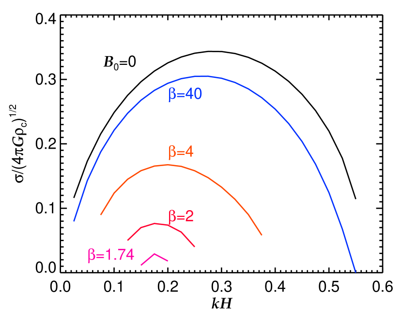
Figure 1: Growth rate $\sigma$ as a function of the wavenumber $kH$ for the fixed boundary. The ordinate is normalized to units of $\sqrt{4\pi G\rho_{c}}$.

The growth rate $\sigma$ has its maximum around $kH\simeq 0.29$ in the absence of the magnetic field ($B_{0}=0$). The growth rate is reduced greatly by the magnetic field having its root fixed at infinity. We find an unstable mode only in the range $0.05<kH<0.4$ for $\beta=4$. The unstable mode disappears when $B_{0}>1.1\sqrt{4\pi\rho_{c}c_{s}^{2}}$, i.e., when the plasma beta is smaller than 1.67 ($\beta<1.67$).

The stabilization due to the magnetic field is shown clearly in Figure 2, where each curve is $\sigma^{2}$ as a function of $1/\beta=B_{0}^{2}/(4\pi\rho_{c}c_{s}^{2})$ for a given $kH$. The square of the growth rate, $\sigma^{2}$, decreases in proportion to $1/\beta$, i.e., $B_{0}^{2}$ in the range $\beta<10$. The proportional constant is larger for a larger $kH$. The dispersion relation is similar to that for the MHD fast wave,

$$\omega^{2}=\left(c_{s}^{2}+\frac{\mbox{\boldmath$B$}_{0}^{2}}{4\pi\rho_{0}}\right)k^{2},$$ (61)

where the wave is assumed to propagate normal to the magnetic field $B$.

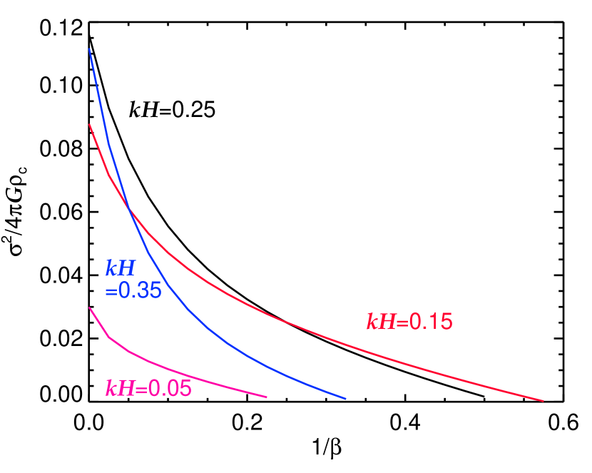
Figure 2: Growth squared as a function of $1/\beta$ for a given $kH$, where $\beta$ denotes the initial plasma beta at the cloud center, $x=y=0$.

The growth rate shows a different dependence on the magnetic field strength when we apply the free boundary condition. Figure 3 is the same as Figure 1 except for the free boundary. Each curve in Figure 3 denotes the growth rate as a function of $kH$ for a given $\beta$ whose value is designated by the same color. The dashed line denotes the growth rate when $\beta=0$, and the value is obtained by extrapolation. As the magnetic field strength increases, the growth rate decreases but remains positive for $kH\leq 0.525$, and therefore the cloud is unstable even when the magnetic field is infinitely strong.

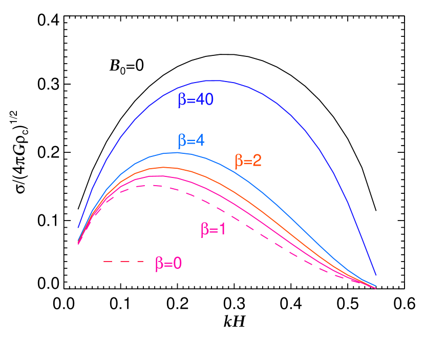
Figure 3: Same as Fig. 1 except for the free boundary.

The result shown in Figure 3 seems to contradict the naive expectation that a subcritical cloud is stable (see, e.g., Nakano & Nakamura, 1978). We explain the apparent discrepancy in the next subsection.

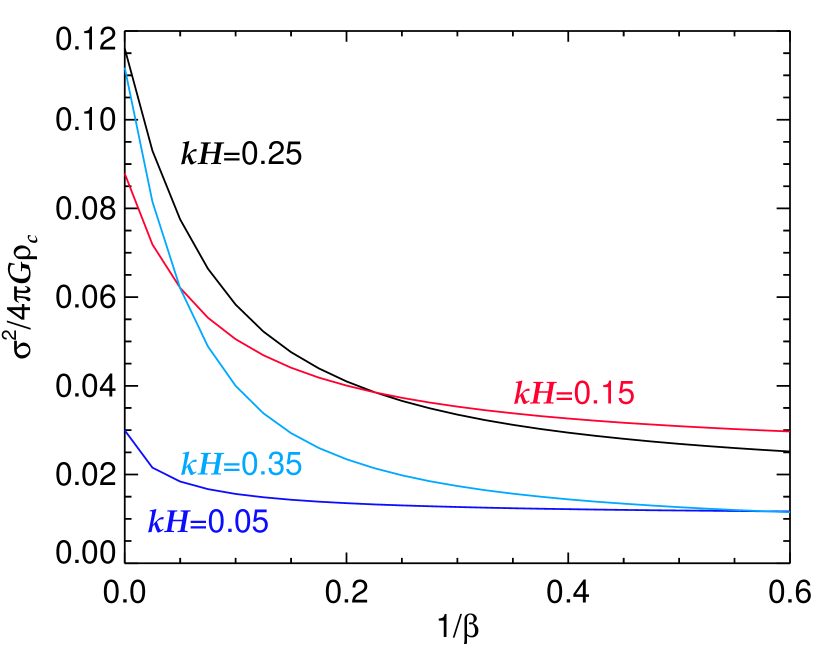
Figure 4: Growth squared as a function of $1/\beta$ for a given $kH$ for the free boundary.

Figure 4 is the same as Figure 2 except for the free boundary. The growth rate approaches a certain value in the limit of large $B_{0}$. The growth rate is well approximated by

$$\sigma^{2}\left(k,B_{0}\right) = [\sigma_{\infty}(k)]^{2}+\left[\sigma^{\prime}(k)\right]^{2}\beta.$$ (62)

The growth rate $\sigma_{\infty}(k)$ is evaluated by a spline fit to the growth rate in the range $0.2\leq\beta\leq 1$. The value of $\sigma_{\infty}(k)$ is shown by the dashed curve in Figure LABEL:growthM.

When $kH$ is smaller, the growth rate is close to the asymptotic value for a weaker magnetic field. This result implies that the magnetic field is bent or compressed little by the unstable perturbation when the initial magnetic field is strong. Otherwise, the distorted magnetic field would induce a strong force acting on the gas. At the same time, the displacement should be appreciable even in the region very far from the cloud center. Otherwise, the growth rate would be independent of the boundary condition in the $x$-direction. We confirm this expectation in the next subsection.

The wavenumber of the most unstable mode is smaller for a larger $B_{0}$. The wavenumber is $kH\simeq 0.29$ for $B_{0}=0$ and $kH\simeq 0.16$ for a small $\beta$. The magnetic field decreases the growth rate and increases the wavelength of a typical perturbation.

The filamentary cloud is stable for any perturbation having a wavenumber larger than $k>k_{\rm cr}=0.565\,H^{-1}$ when $B_{0}=0$. When the free boundary is applied, the critical wavenumber is slightly reduced, i.e., $k_{\rm cr}\,H^{-1}\simeq 0.51$ for a large $B_{0}$. The critical wavenumber is evaluated from the high resolution computation of $\Delta x=\Delta y=0.3H$ and $n_{x}=n_{y}=80$.

3.2 Eigenmode

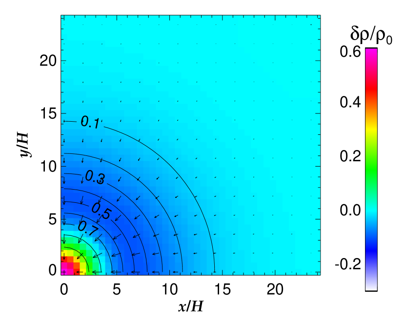
Figure 5: Eigenmode for $B_{0}=0$ and $kH=0.2$. The color denotes $\delta\varrho/\rho_{0}$, while the contours are of $-\xi_{z}/H$. The arrows indicate $(\xi_{x},\xi_{y})$.

First, based on our stability analysis, we review the unstable perturbation in the absence of the magnetic field. When $B_{0}=0$, both the growth rate and the eigenmode depend little on the boundary condition. Figure 5 shows the unstable mode for the fixed boundary when $B_{0}=0$ and $kH=0.2$. The values are normalized so that $\xi_{z}=-H$ at the origin. The arrows indicate the displacement $(\xi_{x},\xi_{y})$, while the contours are of $\xi_{z}$. The density perturbation $\delta\varrho/\rho_{0}$ is representing according to the color scale given in the right panel. The displacement is very small in the region $\sqrt{x^{2}+y^{2}}>15H$ when the fixed boundary is set as $x=24H$ and $y=24H$. Thus, the growth rate depends little on the outer boundary condition. The gas concentrates towards the origin and the density decreases in the surrounding gas.

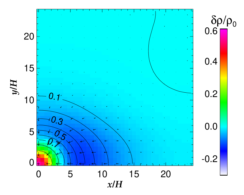
Figure 6: Eigenmode for the fixed boundary. The wavenumber and the initial plasma beta are set as $kH=0.2$ and $\beta=100$, respectively. The notation is the same as that of Fig. 5.

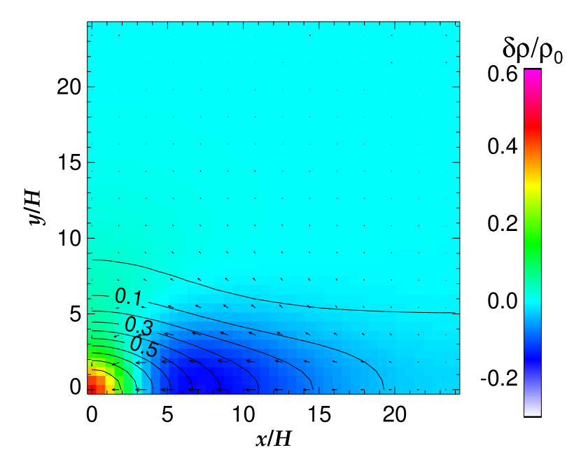
Figure 7: Same as Fig. 6 except $\beta=16.67$.

Low-density gas is affected by a magnetic field even when the magnetic field is very weak. Figures 6 and 7 are the same as Figure 5, except the initial plasma betas are $\beta=100$ and 16.67 at the cloud center, respectively. The displacement in the $y$-direction is greatly suppressed, especially in the region of large $y$, since it is perpendicular to the magnetic field. Also, the displacement along the cloud axis ($\xi_{z}$: contour lines) is restricted in the region $|y|<8H$ when $\beta=$ 16.67 . It should be noted that $|\xi_{x}|$ is large in the more extended region in the $x$-direction (along the initial magnetic field) than in the absence of the magnetic field. The gas in the region far from the cloud axis is anchored through the magnetic field by the gas around the cloud center. The magnetic fields in Figures 6 and 7 are loosely bent because the roots are fixed on the outer boundary. The magnetic tension works against fragmentation as expected from the variational principle shown in Appendix A. When the initial magnetic field is stronger, the density perturbation is smaller. We again note that the unstable mode is normalized so that the displacement in the $z$-direction is $\xi_{z}(0,0)=-H$.

Figure 8 is the same as Figure 5 except for the equilibrium model, $\beta=2$. The growth rate is much smaller than that for $B_{0}=0$. The displacement is negligibly small in the region $|y|>5H$, where the magnetic flux tube is subcritical. Note that the displacement is toward the origin along the $x$-axis, while it is away from the origin in the $y$-direction. The $\delta\varrho>0$ region is concentrated around the $y$-axis. This density enhancement is mainly due to the $x$- and $z$-components of the displacement. The $y$-component elongates the density enhancement along the $y$-axis.

Figure 8: Same as Fig. 6 except $\beta=2$.

Not only the growth rate but also the eigenfunction depends on the boundary condition. Figure 9 is the same as Figure 6 except the boundary is free and $\beta=4$. The $y$-component of the displacement has a large value even in the region of $x\gtrsim 10H$. The $z$-component of the displacement changes its sign around $y\simeq 9H$.

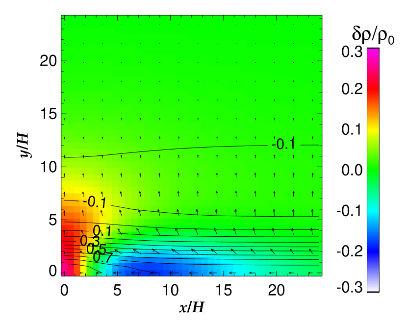
Figure 9: Eigenmode for the free boundary. The wavenumber and initial plasma beta are set as $kH=0.2$ and $\beta=4$, respectively. The notation is the same as that of Fig. 5.

When the free boundary is applied, the magnetic field lines can rotate freely around the $x$-axis, as shown in Figure 10. Figure 10 shows the perturbation in the $x=0$ plane for the eigenmode depicted in Figure 9. The arrows indicate the displacement, while the color indicates the relative change in the density, $\delta\rho(0,y,z)/\rho_{0}(0,y,z)$. The contours depict the change in the $x$-component of the magnetic field in intervals of $\delta B_{x}(0,y,z)/B_{0}=0.04$. The displacement is essentially incompressible circulation, which deforms the shape of the filamentary cloud. The cloud diameter increases in the $y$-direction at the points where the density increases. In other words, each dense fragment expands in the $y$-direction. It should be noted that the cloud changes its form in the opposite way when the magnetic field is absent or longitudinal. In that case, the cloud diameter decreases at the points where the density increases (see Figure 5). The density enhancement is mainly due to the displacement along the density gradient $\mbox{\boldmath$\xi$}\cdot\mbox{\boldmath$\nabla$}\rho_{0}$. The compression by the displacement perpendicular to the magnetic field is very weak. Compared with the relative change in the density, the change in the magnetic field is much smaller, i.e., $\left|\delta B_{x}/B_{0}\right|\ll|\delta\rho|/\rho_{0}$.

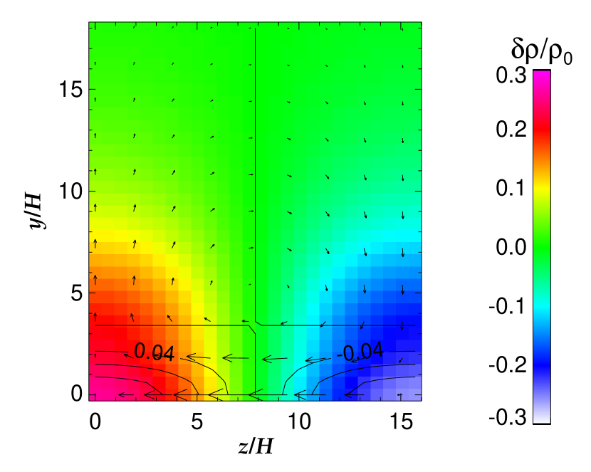
Figure 10: The displacement in the $x=0$ plane is shown by the arrows for the eigenmode shown in Fig. 9. The color indicates $\delta\rho(0,y,z)/\rho_{0}(0,y,z)$, while the contours are of $\delta B_{x}(0,y,z)/B_{0}$.

Figures 11 is the same as Figure 9 except $\beta$ = 2. The $z$-component of displacement, $\xi_{z}$, changes sign around $y\simeq 12H$. In contrast to the case of the fixed boundary, the $y$-component of displacement is appreciably large in the low-density region. This is because magnetic tension does not arise by displacement when the free boundary is applied.

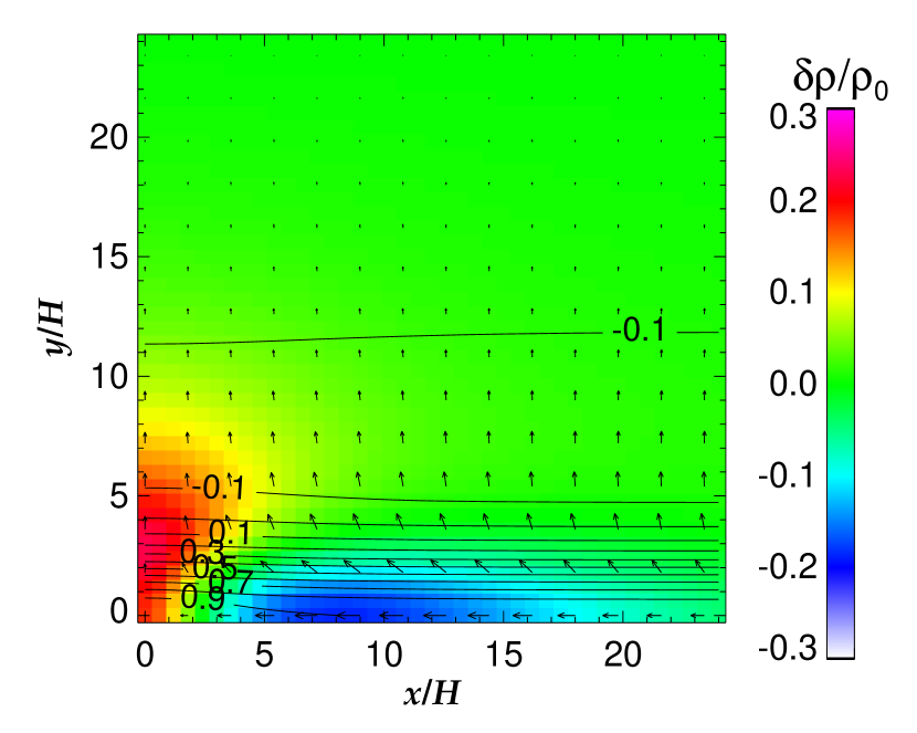
Figure 11: Same as Fig. 9 except $\beta=2$.

Figure 12 is the same as Figure 9 except $\beta=0.2$. Although the model cloud is subcritical [see Equation (13)], it is unstable. In other words, it is unstable though the magnetic energy dominates over the gravitational energy.

The free boundary allows rearrangement of the magnetic flux tubes in the $yz$ plane while keeping them straight and therefore without induction of magnetic force. The rearrangement reduces the gravitational energy if it gathers more massive tubes, i.e., those tubes initially located near the cloud axis. The gravitational energy release by the rearrangement depends little on the magnetic field. Thus, the growth rate also depends little on $B_{0}$. This mode is not taken into account in Hanawa & Tomisaka (2015), where the mass-to-flux ratio is assumed to be constant in the stability analysis for simplicity.

Although it is due to the self-gravity of the gas, the instability may not result in dynamical collapse, since the displacement is dominated by circulation. The change in gravity is due to the change in the cloud shape. This instability is similar to that found by Nagai, Inutsuka & Miyama (1998). They found that a magnetized sheet-like cloud is unstable due to the self-gravity even when the cloud magnetic field is very strong. We discuss the choice of boundary conditions in the next section.

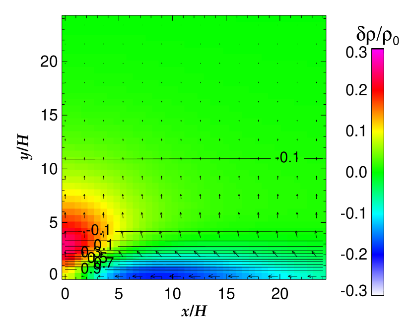
Figure 12: Same as Fig. 9 except $\beta=0.2$.

4 DISCUSSIONS

We used a very simplified model for the filamentary cloud in our stability analysis. The medium is approximated by an isothermal gas and turbulence is not taken into account. These simplifications make the MHD stability analysis feasible. When the magnetic field is perpendicular to the cloud axis, we need to distinguish the direction parallel to the field line from that perpendicular to both the cloud axis and the magnetic field. Thus, the normal mode analysis cannot be reduced to a one-dimensional problem, unlike the previous MHD stability analyses for a filamentary cloud by Hanawa et al. (1993); Fiege & Pudritz (2000). Our analysis is formulated as a two-dimensional problem and its computational cost is much higher than that for a one-dimensional problem.

Our analysis has shown that the stability depends critically on the boundary assumed for $x^{2}+y^{2}\rightarrow\infty$. The dependence comes from the fact that the filamentary clouds are connected with the outer boundary through the magnetic field line. The cloud is stable if the magnetic field is substantial and the field lines are fixed in a region far from it. On the other hand, the cloud is unstable even when the magnetic field is extremely strong if the field lines are free to move in a region far from it. This implies that the magnetic field outside the cloud is important for the stability. Such a dependence on the outer boundary was not found in the previous MHD analysis (e.g., Hanawa et al., 1993), since the magnetic field lines were confined within the cloud.

In this section, we discuss numerical accuracy in §4.1 and the effects of magnetic field orientation in §4.2.

4.1 Numerical Accuracy

First we examine the accuracy of the growth rate obtained in our numerical analysis. The numerically obtained values should contain some numerical errors due to the finite spatial resolution, $\Delta x=\Delta y=0.6H$. The spatial resolution is only moderately high because the full width at half maximum (FWHM) of the model cloud is $3.641H$. Despite the moderate spatial resolution, matrix $A$ has dimension

$$n_{A} = 3n_{x}n_{y}+2n_{x}+2n_{y}+1=4961,$$ (63)

so solving the eigenvalue problem takes considerable computation time. The computation time is roughly proportional to $n_{x}^{3}n_{y}^{3}$ since the computation time increases in proportion to $n_{A}^{3}$. Hence, it is not easy to achieve higher spatial resolution to reduce the numerical error in our 2D analysis.

We examine the case of $B_{0}=0$ to assess the error due to the finite spatial resolution. When $B_{0}=0$, the equilibrium model is symmetric around the axis and therefore the perturbation is also symmetric. The eigenvalue problem reduces to a 1D problem, as shown in Appendix B. We can achieve very high spatial resolution to eliminate the numerical error due to the finite spatial resolution.

As shown in Appendix C, our numerical method has second-order accuracy in space. The numerical error is proportional to the square of the spatial resolution, $\Delta r$, in our 1D analysis and is evaluated as

$$\frac{\Delta(\sigma^{2})}{4\pi G\rho_{c}}\simeq 3.4\times 10^{-4}\left(\frac{\Delta r}{0.1H}\right)^{2},$$ (64)

from Figure 2 for the mode of $kH=0.25$.

Table 13 compares the growth rate squared, $\sigma^{2}$, obtained in our 1D and 2D analyses. The spatial resolutions are $\Delta r=0.1H$ and $\Delta x=\Delta y=0.6H$ in the 1D and 2D analyses, respectively. Despite the large difference in the formal spatial resolutions, the difference in the obtained growth rates is as small as

$$-1.1\times 10^{-3}<\frac{\left(\sigma^{2}\right)_{\rm 2D}-\left(\sigma^{2}\right)_{\rm 1D}}{4\pi G\rho_{c}}<-3\times 10^{-4}.$$ (65)

This difference is comparable to the expected numerical error for the growth rate obtained in our 1D analysis. Thus, we estimate that the numerical error of our 2D analysis is about $\Delta\left(\sigma^{2}\right)\simeq 10^{-3}(4\pi G\rho_{0})$. Although the formal spatial resolution is $\Delta x=\Delta y=0.6H$, the effective spatial resolution is likely to be higher since the displacement is evaluated not only on the $x$- and $y$-axes but at various points in the $xy$ plane.

The accuracy mentioned above is consistent with the spatial extent of the displacement. As shown in Figure 5, the displacement is large in the region $\sqrt{x^{2}+y^{2}}\lesssim 10H$, which is covered by $16\times 16$ grid points. The error due to the finite difference is estimated to be $\approx[1/(2\times 16)]^{-2}\simeq 10^{-3}$, since the difference equations are of second-order accuracy. The factor 2 is introduced to take account of the region of negative $x$ and $y$.

The presence of the magnetic field may increase the numerical error since the magnetic field confines the displacement in an especially narrow region when the fixed boundary condition is applied. Nevertheless, the error is likely to be moderate since the eigenmode is well resolved, as shown in the previous section. We expect that the numerical error is smaller than $\Delta(\sigma^{2})<5\times 10^{-3}(4\pi G\rho_{c})$ and does not have serious effects on our analysis.

4.2 Effects of Magnetic Field Perpendicular to the Cloud

Next we discuss the dependence of the instability on the direction of the magnetic field. As shown in the previous section, the magnetic field works against fragmentation and reduces the growth rate of instability when it is perpendicular to the cloud axis. On the other hand, the magnetic field does not suppress the instability when it is parallel to the cloud axis (see, e.g., Stodólkiewicz, 1963; Hanawa et al., 1993). A toroidal or helical magnetic field stabilizes fragmentation of the cloud and reduces the growth rate of the sausage (axisymmetric) mode (Fiege & Pudritz, 2000), although it induces the kink (non-axisymmetric) mode. These modes are characterized by the geometry of the magnetic field, namely, whether the magnetic field is bent or compressed by the fragmentation.

Before applying our analysis to observed filamentary molecular clouds, we need to discuss the boundary conditions employed in our analysis. As shown in the previous section, the boundary conditions greatly affect the instability. When the free boundary condition is applied, the filamentary cloud is unstable even when the magnetic field is extremely strong. In other words, no magnetic field can suppress the instability if the displacement does not vanish in the region very far from the cloud. The unstable mode exists because the density decreases in proportion to $\rho_{0}\propto r^{-4}$, where $r$ denotes the radial distance from the cloud axis. In our model, the displacement travels from the cloud center to infinity through the Alfvén wave in a finite time,

$$\tau_{\rm A} = \int_{0}^{\infty}\frac{\sqrt{4\pi\rho_{0}}}{B_{0}}dx=\frac{2\pi\sqrt{2\pi\rho_{c}}H}{B_{0}}.$$ (66)

The Alfvén transit time may be much longer in reality because the density is higher or the magnetic field is weaker in the region far from the cloud. Palmeirim et al. (2013) reported that the mean radial column density fits a Plummer-like density distribution,

$$\rho_{\rm P} = \frac{\rho_{c}}{\left[1+\left(r/R_{\rm flat}^{2}\right)\right]^{p/2}},$$ (67)

where $R_{\rm flat}$ denotes the radius of the inner flat region. In the best-fit model, $R_{\rm flat}=0.07\pm 0.02~{}\mbox{pc}$ and $p=2.0\pm 0.4$ for the B211 filament. The density slope is significantly shallower than that for the isothermal equilibrium, $p=4$. Our model cloud is highly idealized, especially in the region very far from the cloud axis. The shallower slope might be due to turbulence, which is likely to be larger in a lower density gas. We again note that the striations running perpendicular to the main filament (see, e.g., Sugitani et al., 2011; Palmeirim et al., 2013) are unlikely to move easily by magnetic force since the Alfvén velocity is lowered by the relatively high density. If the Alfvén transit timescale is longer than the free-fall timescale, the fixed boundary condition may be appropriate. We need to account for the low-density region surrounding the filamentary cloud when applying our analysis.

Tomisaka (2014) made a model for a filamentary cloud in which the magnetic field lines lie in the plane perpendicular to the cloud axis. In his equilibrium model, the cloud is supported in part by the magnetic tension. The magnetic field is weaker at a greater distance from the cloud axis. In other studies with 3D MHD simulations, the magnetic fields are not uniform around the filamentary clouds formed (see, e.g., Nakamura & Li, 2008; Klassen, Pudritz & Kirk, 2017). If the density is very low in the periphery of the filamentary cloud, the magnetic field should be quasi force-free and thus nearly straight. It is also well known that the magnetic field is stronger where the column density is higher (see, e.g., Li et al., 2014).

Our result for the free boundary is quite similar to those obtained by Nagai, Inutsuka & Miyama (1998) and Fiege & Pudritz (2000), who studied the stability of an isothermal gas layer and a filament confined by the outer gas pressure, respectively.

Nagai, Inutsuka & Miyama (1998) assumed that the magnetic field is uniform and parallel to the gas midplane. This gas layer suffers from two types of instability: fragmentation due to displacement along the magnetic field and distortion of the surface layer. When the gas layer is thick and consequently mostly gravitationally bound, the instability due to displacement dominates. When the gas layer is thin and consequently pressure bound, the distortion dominates and the gas layer fragments into filaments. The magnetic fields remain straight as the instability due to distortion develops. As a result, the magnetized gas sheet is unstable and the growth rate remains constant in the limit of a strong magnetic field, as in the case of the free boundary condition in our stability analysis. Although the latter instability is due to the self-gravity, the filaments formed do not collapse directly, since the filaments expand in the direction normal to the initial sheet by the instability. It should again be noted that this instability develops even when the sheet is extremely thin and the self-gravity is not important. It seems that the this instability is analogous to the instability for the free boundary.

Fiege & Pudritz (2000) showed that their truncated Ostriker model is unstable against fragmentation. The model filamentary cloud is assumed to be surrounded by hot gas of negligibly small density. Their initial model was similar to that of Nagai, Inutsuka & Miyama (1998) except for the geometry and the magnetic field. When the pressure of the hot gas is comparable to that at the filament center, circulation dominates in the unstable mode, as in our model for the free boundary (see their Figure 4). Each dense clump expands in the radial direction as a result of the instability. The change in the gravitational potential is mainly due to that in the boundary between hot and cold gases (i.e., the boundary of the dense gas), as in our free boundary model. It seems that a relatively strong magnetic field increases the effective temperature of the gas through magnetic pressure and therefore we obtain similar results.

As shown in §2, the model cloud is subcritical when the plasma beta is as low as 0.405. It is well known that molecular clouds collapse dynamically only when the cloud is supercritical. Thus, the subcritical cloud forms clumps supported in part by the magnetic force, not by dynamically collapsing cores. In other words, fragmentation does not result in direct star formation.

The above argument implies that subcritical clumps can be formed via fragmentation of a filamentary cloud if the free boundary is the case. A subcritical filamentary cloud may suffers from fragmentation instability. The instability is not likely to result in the dynamical collapse to form gravitationally bound clumps supported mainly by magnetic field. Such clumps may form stars through quasi-static contraction, i.e., after substantial amount of magnetic field is liberated through the ambipolar diffusion.

Our analysis suggests to study low density region surrounding a filamentary cloud. Motion in the high-density region may propagate into the outer region through the Alfvén wave, when the filamentary cloud fragments. It would be meaningful to observe the velocity field around the filamentary structure. The motion perpendicular to the magnetic field may contain information on the motion in the dense region. The Alfvén speed is proportional to the inverse square root of the density ($\propto\rho^{-1/2}$). Thus the motion is faster when the density is lower. The density distribution may be controlled by turbulence. If it is the case, turbulence may affect the stability of a filamentary cloud indirectly through the boundary condition.

Appendix A Variational Principle

In this appendix, we prove that the growth rate is either real or pure imaginary. For this purpose, we integrate the inner product of Equation (30) and $\mbox{\boldmath$\xi$}^{*}$ over the volume, where the asterisk denotes the complex conjugate. The integral is expressed as

$$\sigma^{2}I = W_{\rm T}+W_{\rm G}+W_{\rm M},$$ (A1)

$$I = \int_{-\infty}^{+\infty}\!\!\!\int_{-\infty}^{+\infty}\!\!\!\int_{0}^{2\pi/k}\rho|\mbox{\boldmath$\xi$}|^{2}dxdydz,$$ (A2)

$$W_{\rm T} = -c_{s}^{2}\int_{-\infty}^{+\infty}\!\!\!\int_{-\infty}^{+\infty}\!\!\!\int_{0}^{2\pi/k}\rho_{0}\mbox{\boldmath$\xi$}^{*}\cdot\mbox{\boldmath$\nabla$}\left(\frac{\delta\rho}{\rho_{0}}\right)dxdydz,$$ (A3)

$$W_{\rm G} = -\int_{-\infty}^{+\infty}\!\!\!\int_{-\infty}^{+\infty}\!\!\!\int_{0}^{2\pi/k}\rho_{0}\mbox{\boldmath$\xi$}^{*}\cdot\mbox{\boldmath$\nabla$}\delta\psi dxdydz,$$ (A4)

$$W_{\rm M} = \int_{-\infty}^{+\infty}\!\!\!\int_{-\infty}^{+\infty}\!\!\!\int_{0}^{2\pi/k}\mbox{\boldmath$\xi$}^{*}\cdot\left(\delta\mbox{\boldmath$J$}\times\mbox{\boldmath$B$}_{0}\right)dxdydz,$$ (A5)

The integral $I$ is real and positive for any $\xi$. The integral $W_{\rm T}$ is also proved to be real and negative, since

$$W_{\rm T} = c_{s}^{2}\int_{-\infty}^{+\infty}\!\!\!\int_{-\infty}^{+\infty}\!\!\!\int_{0}^{2\pi/k}\mbox{\boldmath$\nabla$}\cdot\left(\rho_{0}\mbox{\boldmath$\xi$}^{*}\right)\left(\frac{\delta\rho}{\rho_{0}}\right)dxdydz$$ (A6)

$$= -c_{s}^{2}\int_{-\infty}^{+\infty}\!\!\!\int_{-\infty}^{+\infty}\!\!\!\int_{0}^{2\pi/k}\frac{|\delta\rho|^{2}}{\rho_{0}}dxdydz.$$ (A7)

Here we use the boundary condition at infinity and Equation (15) in the integration by parts. Similarly, the integral $W_{\rm G}$ is proved to be real and positive for any perturbation, since

$$W_{\rm G} = \int_{-\infty}^{+\infty}\!\!\!\int_{-\infty}^{+\infty}\!\!\!\int_{0}^{2\pi/k}\mbox{\boldmath$\nabla$}\cdot\left(\rho_{0}\mbox{\boldmath$\xi$}^{*}\right)\delta\psi dxdydz$$ (A8)

$$= -\int_{-\infty}^{+\infty}\!\!\!\int_{-\infty}^{+\infty}\!\!\!\int_{0}^{2\pi/k}\delta\rho^{*}\delta\psi dxdydz$$ (A9)

$$= -\frac{1}{4\pi G}\int_{-\infty}^{+\infty}\!\!\!\int_{-\infty}^{+\infty}\!\!\!\int_{0}^{2\pi/k}\Delta\delta\psi^{*}\delta\psi dxdydz$$ (A10)

$$= \frac{1}{4\pi G}\int_{-\infty}^{+\infty}\!\!\!\int_{-\infty}^{+\infty}\!\!\!\int_{0}^{2\pi/k}\left|\mbox{\boldmath$\nabla$}\delta\psi\right|^{2}dxdydz.$$ (A11)

The integral $W_{\rm M}$ is proved to be real and negative, since

$$W_{\rm M} = -\int_{-\infty}^{+\infty}\!\!\!\int_{-\infty}^{+\infty}\!\!\!\int_{0}^{2\pi/k}\delta\mbox{\boldmath$J$}\cdot\left(\delta\mbox{\boldmath$\xi$}^{*}\times\mbox{\boldmath$B$}_{0}\right)dxdydz$$ (A12)

$$= -\frac{1}{4\pi}\int_{-\infty}^{+\infty}\!\!\!\int_{-\infty}^{+\infty}\!\!\!\int_{0}^{2\pi/k}\mbox{\boldmath$\nabla$}\times\delta\mbox{\boldmath$B$}\cdot\left(\delta\mbox{\boldmath$\xi$}^{*}\times\mbox{\boldmath$B$}_{0}\right)dxdydz$$ (A13)

$$= -\frac{1}{4\pi}\int_{-\infty}^{+\infty}\!\!\!\int_{-\infty}^{+\infty}\!\!\!\int_{0}^{2\pi/k}\delta\mbox{\boldmath$B$}\cdot\mbox{\boldmath$\nabla$}\times\left(\delta\mbox{\boldmath$\xi$}^{*}\times\mbox{\boldmath$B$}_{0}\right)dxdydz$$ (A14)

$$= -\frac{1}{4\pi}\int_{-\infty}^{+\infty}\!\!\!\int_{-\infty}^{+\infty}\!\!\!\int_{0}^{2\pi/k}\left|\delta\mbox{\boldmath$B$}\right|^{2}dxdydz.$$ (A15)

Either $\xi$ or $\delta\mbox{\boldmath$B$}$ is assumed to vanish at infinity. $\xi$ corresponds to the fixed boundary, whereas $\delta\mbox{\boldmath$B$}$ corresponds to the free boundary. Thus, the square of the growth rate, $\sigma^{2}$, should be real since

$$\sigma^{2} = \frac{W_{\rm T}+W_{\rm G}+W_{\rm M}}{I}.$$ (A16)

It is also clear from Equation (A16) that the filament can be unstable only through the self-gravity, $W_{\rm G}$.

Appendix B Matrix Elements

This appendix describes each component of the vector $\zeta$, and matrixes $A$, $B$, and $C$.

The $m$-th element of the vector $\zeta$ is set so that

$$\zeta_{m} = \xi_{x,i-1/2,j},\hskip 10.0pt(i=1,2,\dots,n_{x}~{}\mbox{and}~{}j=0,1,\dots,n_{y})$$ (B1)

$$m = i+n_{x}j,$$ (B2)

for $1\leq m\leq n_{x}\left(n_{y}+1\right)$. Indexes $i$ and $j$ are derived from $m$ by

$$i = [(m-1)\,(\mbox{mod}\,n_{x})]+1,$$ (B3)

$$j = \frac{m-i}{n_{x}}.$$ (B4)

Other elements of the vector, $\zeta$, are set as

$$\zeta_{m} = \xi_{y,i,j-1/2},\hskip 10.0pt(i=0,1,\dots,n_{x}~{}\mbox{and}~{}j=1,2,\dots,n_{y})$$ (B5)

$$m = i+1+\left(n_{x}+1\right)\left(j-1\right)+n_{x}\left(n_{y}+1\right),$$ (B6)

$$i = \left\{\left[m-n_{x}\left(n_{y}+1\right)-1\right]\,\left(\mbox{mod}\,n_{x}+1\right)\right\}+1$$ (B7)

$$j = \frac{m-i-n_{x}\left(n_{y}+1\right)}{n_{x}+1},$$ (B8)

for $n_{x}\left(n_{y}+1\right)<m\leq 2n_{x}n_{y}+n_{x}+n_{y}$, and

$$\zeta_{m} = \xi_{z,i,j},\hskip 10.0pt(i=0,1,\dots,n_{x}~{}\mbox{and}~{}j=0,1,\dots,n_{y})$$ (B9)

$$m = i+1+\left(n_{x}+1\right)j+2n_{x}n_{y}+n_{x}+n_{y},$$ (B10)

for $2n_{x}n_{y}+n_{x}+n_{y}<m\leq 3n_{x}n_{y}+2n_{x}+2n_{y}+1$. The changes in the density, current density, and gravity are evaluated once the displacement, $\zeta$, is given. All the forces are proportional to the displacement $\zeta$, and the magnetic force is also proportional to $B_{0}^{2}$. Hence, Equations (56) through (58) are transformed into Equation (59).

The $m$-th column of matrix $A$ is evaluated by the following procedure. First we compute $\delta\varrho_{i,j}$ for all pairs of $i$ and $j$ according to Equation (36) for $\zeta_{m}=1$ and $\zeta_{m^{\prime}}=0$ for $m^{\prime}\neq m$. Note that the change in the density, $\delta\varrho_{i,j}$, vanishes for the given displacement except at a few points. Then the change in the gravitational potential is evaluated according to Equation (38). The Green’s function is defined as the solution of

$$\frac{G_{i+1,j,i^{\prime},j^{\prime}}-G_{i-1,j,i^{\prime},j^{\prime}}}{\Delta x^{2}}+\frac{G_{i,j+1,i^{\prime},j^{\prime}}-G_{i,j-1,i^{\prime},j^{\prime}}}{\Delta y^{2}}-\left(\frac{2}{\Delta x^{2}}+\frac{2}{\Delta y^{2}}+k^{2}\right)G_{i,j,i^{\prime},j^{\prime}} = 4\pi G\delta_{i,i^{\prime}}\delta_{j,j^{\prime}},$$ (B11)

where $\delta_{i,i^{\prime}}$ and $\delta_{j,j^{\prime}}$ denote the Kronecker’s delta. The solution should satisfy the boundary condition on the $y$-axis ($x=0$),

$$G_{-1,j,i^{\prime},j^{\prime}} = G_{1,j,i^{\prime},j^{\prime}},$$ (B12)

and that on the $x$-axis ($y=0$),

$$G_{i,-1,i^{\prime},j^{\prime}} = G_{i,1,i^{\prime},j^{\prime}},$$ (B13)

for any $i$, $j$, $i^{\prime}$, and $j^{\prime}$. The boundary conditions are taken into account by the mirror image method: we superimpose the solutions for the mirror images in which the boundary conditions are set as $G_{i,j,i^{\prime},j^{\prime}}=0$ in the region $|i-i^{\prime}|\Delta x\gg H$ or $|j-j^{\prime}|\Delta y\gg H$. We use Gauss-Seidel iteration to obtain the Green’s function with the boundary condition set as $|i-i^{\prime}|=2n_{x}$ and $|j-j^{\prime}|=2n_{y}$. Using $\delta\varrho_{i,j}$ and $\delta\psi_{i,j}$, we evaluate the pressure force and gravity in the right-hand side of Equations (56) through (58) to obtain the $m$-th column of matrix $A$. Equations (56), (57), and (58) provide the first $n_{x}\left(n_{y}+1\right)$, second $\left(n_{x}+1\right)n_{y}$, and last $(n_{x}+1)(n_{y}+1)$ components of the $m$-th column of $A$. The row number is evaluated from $i$ and $j$ according to Equations (B2), (B6), and (B10).

Matrix $B$ is diagonal with diagonal elements representing the equilibrium density, $\rho_{0}$, at the point where the displacement is evaluated.

Matrix $C$ is obtained in a similar manner. The $m$-th column of $C$ denotes the magnetic force when $\zeta_{m^{\prime}}=\delta_{m,m^{\prime}}$ and $B_{0}=\sqrt{4\pi\rho_{c}}c_{s}$.

Appendix C Case of No Magnetic Field

In this appendix, we examine the instability of an unmagnetized filamentary cloud. When $\mbox{\boldmath$B$}_{0}=0$, the equilibrium model is symmetric around the axis. Hence, the unstable mode is also symmetric around the axis. Then, density, displacement, and potential can be described as

$$\rho = \rho_{0}+\delta\varrho(r)\cos kz,$$ (C1)

$$\xi = \xi_{r}(r)\cos kz\mbox{\boldmath$e$}_{r}+\xi_{z}(r)\sin kz\mbox{\boldmath$e$}_{z},$$ (C2)

$$\psi = \psi_{0}+\delta\psi(r)\cos kz,$$ (C3)

in cylindrical coordinates $(r,\theta,z)$. The perturbation equations are written as

$$\delta\varrho = -\frac{1}{r}\frac{\partial}{\partial r}\left(r\rho_{0}\xi_{r}\right)-k\rho_{0}\xi_{z},$$ (C4)

$$\sigma^{2}\rho_{0}\xi_{r} = -c_{s}^{2}\rho_{0}\frac{\partial}{\partial r}\left(\frac{\delta\varrho}{\rho_{0}}\right)-\rho_{0}\frac{\partial}{\partial r}\delta\psi,,$$ (C5)

$$\sigma^{2}\rho_{0}\xi_{z} = kc_{s}^{2}\delta\varrho+k\rho_{0}\delta\psi,$$ (C6)

$$4\pi G\delta\varrho = \frac{1}{r}\frac{\partial}{\partial r}\left(r\frac{\partial}{\partial r}\delta\psi\right)-k^{2}\delta\psi.$$ (C7)

From Equations (C5) and (C6), we obtain

$$\frac{\partial\xi_{z}}{\partial r}+k\xi_{r} = 0.$$ (C8)

We solve the perturbation equations numerically by the following procedure. First we discretize Equation (C8) in the form

$$\xi_{r,j+1/2} = -\frac{1}{k\Delta r}\left(\xi_{z,j+1}-\xi_{z,j}\right),$$ (C9)

where $\xi_{r,j+1/2}$ and $\xi_{z,j}$ denote the values at $r=r_{j+1/2}=(j+1/2)\Delta r$ and $r=r_{j}=j\Delta r$, respectively. The change in density is evaluated as

$$\delta\varrho_{j} = -\frac{1}{r_{j}\Delta r}\left(r_{j+1/2}\rho_{0,j+1/2}\xi_{r,j+1/2}-r_{j-1/2}\rho_{0,j-1/2}\xi_{r,j-1/2}\right)-k\rho_{0,j}\xi_{z,j}$$ (C10)

by discretizing Equation (C4), where $\delta\varrho_{j}$ and $\rho_{0,j+1/2}$ denote the values at $r=r_{j}$ and $r_{j+1/2}$, respectively. The change in the gravitational potential, $\delta\psi$, is obtained by solving the discretized Poisson equation

$$4\pi G\delta\varrho_{j} = \left\{\begin{array}[]{ll}\displaystyle 2\frac{\delta\psi_{1}-\delta\psi_{0}}{\Delta r^{2}}-k^{2}\delta\psi_{0}&\hskip 20.0pt(j=0)\\ \displaystyle-\frac{r_{j+1/2}\delta\psi_{j+1}-2r_{j}\delta\psi_{j}+r_{j-1/2}\delta\psi_{j-1}}{r_{j}\Delta r^{2}}-k^{2}\delta\psi_{j}&\hskip 20.0pt(j=1,2,\dots,n)\end{array}\right.,$$ (C13)

with the boundary condition

$$\delta\psi_{n+1}=\left(1+k\Delta r\right)^{-1}\delta\psi_{n},$$ (C14)

where $j=n$ denotes the outermost grid point while $j=n+1$ does the one adjacent outside.

Using Equations (C9) through (C14), we derive $\xi_{r,j-1/2}$, $\delta\varrho_{j}$, and $\delta\psi_{j}$ for a given set of $\xi_{z,j}$. Then we can evaluate the right-hand side of Equation (C6) in the form of

$$\sigma^{2}\rho_{0,j}\xi_{z,j} = \sum_{i}F_{ji}\xi_{z,i}.$$ (C15)

The growth rate $\sigma$ is numerically obtained by using the Linear Algebra Package, LAPACK (Anderson et al., 1999)).

Figure 13: Dependence of the growth rate squared on the spatial resolution for $B_{0}=0$ and $kH=0.25$.

In this 1D stability analysis, we can evaluate the numerical error due to the discretization. Figure 13 shows $\sigma^{2}$ as a function of the spatial resolution $\Delta r$ for the mode $kH=0.25$. The outer boundary is placed at $r=60H$, which is far away enough and does not affect the result. The discretization is of second-order accuracy and the growth rate is expressed as

$$\sigma^{2}(\Delta r;kH=0.25) = 4\pi G\rho_{c}\left[0.114803+3.44\times 10^{-4}\left(\frac{\Delta r}{0.1H}\right)^{2}\right].$$ (C16)

We conclude that the growth rate is highly accurate when $\Delta r=0.1~{}H$ in the1D analysis.

Table 2 compares the growth rates obtained in our 2D analysis with the growth rates in our 1D analysis for various $kH$. The middle column lists $\sigma^{2}$ values obtained in the 1D analysis, while the right column lists those obtained in the 2D analysis for $B_{0}=0$. The spatial resolution is $\Delta r=0.1~{}H$ in the 1D analysis and $\Delta x=\Delta y=0.6~{}kH$ in the 2D analysis. The outer boundary is set as $r=60~{}H$ in the 1D and $x~{}\mbox{or}~{}y=24.3~{}H$ in the 2D analysis. Since the difference is small, we conclude that our 2D analysis gives a reliable growth rate at least for $B_{0}=0$.

Table 2: Comparison of Growth Rates Squared, $\sigma^{2}$, Obtained in the 1D and 2D Analyses.

$kH$	1D	2D
0.05	0.02962	0.02995
0.10	0.06135	0.06186
0.15	0.08720	0.08785
0.20	0.10528	0.10606
0.25	0.11515	0.11606
0.30	0.11684	0.11787
0.35	0.11059	0.11173
0.40	0.09666	0.09790
0.45	0.07534	0.07667
0.50	0.04690	0.04831

References

- Anderson et al. (1999) Anderson, E., Bai, Z., Bischof, C., Blackford, S., Demmel, J., Dongara, J., Du Croz, J., Greenbaum, A., Hammarling, S., McKenney, A., Sorensen, D. 1999, LAPACK Users’ Guide, 3rd ed. http://www.netlib.org/lapack/lug/
- André et al. (2014) André P., Di Francesco J., Ward-Thompson D. 2014 Protostars and Planets VI ed H. Beuther et al. (Tucson, AZ: Univ. Arizona Press) 27
- Fiege & Pudritz (2000) Fiege, J.D., Pudritz, R.E. 2000, MNRAS, 311, 105
- Hanawa et al. (1993) Hanawa T., Nakamura F., Matsumoto, T., et al. 1993, ApJ, 404, L83
- Hanawa & Tomisaka (2015) Hanawa, T. and Tomisaka, K. 2015 ApJ 801 11
- Klassen, Pudritz & Kirk (2017) Klassen, M., Pudritz, R.E., Kirk, H. 2017 MNRAS, 465, 2254
- Kusune et al. (2016) Kusune, T., Sugitani, K., Nakamura, F., Watanabe, M., Tamura, M. Kwon, J., Sato, S. 2016 ApJ, 803, L23
- Larson (2003) Larson R. B. 2003 RPPh, 66, 1651
- Li et al. (2013) Li H.-b., Fang M., Henning T. and Kainulainen J. 2013 MNRAS, 436, 3707
- Li et al. (2014) Li H.-B., Goodman A., Sridharan T. K. et al 2014 Protostars and Planets VI ed H. Beuther et al.(Tucson, AZ: Univ. Arizona Press) 27