Thermal properties of graphene from path-integral simulations

Abstract

Thermal properties of graphene monolayers are studied by path-integral molecular dynamics (PIMD) simulations, which take into account the quantization of vibrational modes in the crystalline membrane, and allow one to consider anharmonic effects in these properties. This system was studied at temperatures in the range from 12 to 2000 K and zero external stress, by describing the interatomic interactions through the LCBOPII effective potential. We analyze the internal energy and specific heat and compare the results derived from the simulations with those yielded by a harmonic approximation for the vibrational modes. This approximation turns out to be rather precise up to temperatures of about 400 K. At higher temperatures, we observe an influence of the elastic energy, due to the thermal expansion of the graphene sheet. Zero-point and thermal effects on the in-plane and “real” surface of graphene are discussed. The thermal expansion coefficient $\alpha$ of the real area is found to be positive at all temperatures, in contrast to the expansion coefficient $\alpha_{p}$ of the in-plane area, which is negative at low temperatures, and becomes positive for $T\gtrsim$ 1000 K.

I Introduction

Graphene has been extensively studied in last years, not only for its remarkable electronic properties,Geim and Novoselov (2007); Castro Neto et al. (2009); Flynn (2011) but also for other features such as elastic and thermal properties. In fact, graphene displays high values of thermal conductivity,Ghosh et al. (2008); Nika et al. (2009); Balandin (2011) as well as large in-plane elastic constants.Lee et al. (2008) The optimum structural arrangement for pure defect-free graphene corresponds to a honeycomb lattice, but departures from this flat structure may significantly affect both its atomic-scale and macroscopic properties.Meyer et al. (2007)

There are several reasons for a graphene sheet to bend and depart from absolute planarity, such as the presence of defects and external stresses.Fasolino et al. (2007); de Andres et al. (2012a) For a perfect two-dimensional (2D) crystalline layer in three-dimensional (3D) space, thermal fluctuations at finite temperatures cause out-of-plane motion of the carbon atoms, and even for $T\to 0$, quantum fluctuations associated to zero-point motion yield a departure of strict planarity of the graphene sheet.Herrero and Ramírez (2016)

Understanding structural and thermal properties of 2D systems in 3D space is a challenge in modern statistical physics.Safran (1994); Nelson et al. (2004); Tarazona et al. (2013) This question has been mainly treated in connection with biological membranes and soft condensed matter.Tarazona et al. (2013); Chacón et al. (2015); Ruiz-Herrero et al. (2012) However, the large complexity of these systems has limited the development of microscopic approaches based on realistic interatomic interactions. Graphene, as a well-characterized crystalline membrane, can be considered as a model system where an atomistic description is possible, paving the path to a better understanding of the physical properties of this kind of systems. In this line, the interest on thermal properties of graphene has risen in the last few years,Amorim et al. (2014); Pop et al. (2012); Wang et al. (2016); Fong et al. (2013); Mann et al. (2016) as is the case of thermal expansion and heat conduction, which have been recently studied both experimentally and theoretically.Balandin (2011); Pop et al. (2012); Alofi and Srivastava (2013, 2014); da Silva et al. (2014); Burmistrov et al. (2016)

Monte Carlo and molecular dynamics simulations have been employed to study finite-temperature properties of graphene. These simulations were based on ab-initio,de Andres et al. (2012b); Shimojo et al. (2008); Chechin et al. (2014) tight-binding,Akatyeva and Dumitrica (2012); Cadelano et al. (2009); Lee et al. (2013); Herrero and Ramírez (2009) and empirical interatomic potentials.Fasolino et al. (2007); Shen et al. (2013); Ramírez et al. (2016); Magnin et al. (2014); Los et al. (2016) In most cases, carbon atoms were described as classical particles, which is reliable at relatively high temperatures (in the order of the Debye temperature of the material), but is not suitable to study thermodynamic variables at low temperature. To take into account the quantum nature of the atomic motion, path-integral simulations are well-suited, since in this procedure nuclear degrees of freedom may be quantized, allowing one to include quantum and thermal fluctuations in many-body systems at finite temperatures.Gillan (1988); Ceperley (1995) Thus, path-integral simulations of a single graphene layer have been recently carried out to study equilibrium properties of this material.Brito et al. (2015); Herrero and Ramírez (2016) In addition to this, nuclear quantum effects have been studied earlier by using a combination of density-functional theory and a quasi-harmonic approximation for vibrational modes in this crystalline membrane.Mounet and Marzari (2005); Shao et al. (2012)

In this paper, the path-integral molecular dynamics (PIMD) method is used to study thermal properties of graphene at temperatures between 12 and 2000 K. Simulation cells of different sizes are considered, as finite-size effects have been found earlier to be important for some equilibrium properties of graphene.Gao and Huang (2014); Los et al. (2016); Herrero and Ramírez (2016) We study the thermal behavior of the graphene surface, taking into account the difference between real surface and projected in-plane area. Particular emphasis is laid on the temperature dependence of the specific heat at low $T$, for which results of the simulations are compared with predictions based on harmonic vibrations of the crystalline membrane.

The paper is organized as follows. In Sec. II, we describe the computational method employed in the simulations. Results for the internal energy of graphene are given in Sec. III. Structural properties such as the in-plane and real area are discussed in Sec. IV. In Sec. V we present results for the specific heat, and in Sec. VI we summarize the main results.

II Computational Method

In this paper we use PIMD simulations to study equilibrium properties of graphene monolayers as a function of temperature. The PIMD method is based on the path-integral formulation of statistical mechanics,Feynman (1972) which has turned out to be a convenient nonperturbative approach to study finite-temperature properties of many-body quantum systems. In this method, the partition function is evaluated through a discretization of the density matrix along cyclic paths, formed by a finite number $N_{\rm Tr}$ (Trotter number) of steps.Feynman (1972); Kleinert (1990) In actual applications of this procedure to numerical simulations, this discretization causes the appearance of $N_{\rm Tr}$ replicas (or beads) for each quantum particle. These replicas are treated in the calculations as classical particles, since the partition function of the real quantum system is isomorph to that of a classical one, obtained by substituting each quantum particle by a ring polymer composed of $N_{\rm Tr}$ particles.Gillan (1988); Ceperley (1995) The dynamics in this procedure is artificial, as it does not reflect the real quantum dynamics of the actual particles. Nevertheless, it is useful for effectively sampling the many-body configuration space, yielding accurate results for time-independent equilibrium properties of the quantum system under consideration. Details on this simulation technique can be found elsewhere.Chandler and Wolynes (1981); Gillan (1988); Ceperley (1995); Herrero and Ramírez (2014)

An important point for this kind of simulations is a reliable description of the interatomic interactions, which have to be as realistic as possible. We obtain a Born-Oppenheimer surface for the nuclear dynamics from the LCBOPII effective potential,Los et al. (2005) as using an ab-initio method would largely reduce the size of the simulation cells to be handled. This is a long-range carbon bond order potential, which has been used to perform classical simulations of carbon-based systems, such as diamond,Los et al. (2005) graphite,Los et al. (2005), liquid carbon,Ghiringhelli et al. (2005a) and more recently graphene.Fasolino et al. (2007); Zakharchenko et al. (2009); Los et al. (2016) It has been used, in particular, to study the carbon phase diagram including graphite, diamond, and the liquid, and displayed its accuracy in a comparison of the predicted graphite-diamond line with experimental results.Ghiringhelli et al. (2005b) The LCBOPII potential has been also found to describe well several properties of graphene, such as Young’s modulus.Zakharchenko et al. (2009); Politano et al. (2012); Ramírez and Herrero (2017) In line with earlier simulations,Ramírez et al. (2016); Herrero and Ramírez (2016); Ramírez and Herrero (2017) the original LCBOPII parameterization was slightly modified to increase the zero-temperature bending constant from 1.1 eV to a more realistic value of 1.49 eV.Lambin (2014) This effective potential has been recently employed to carry out PIMD simulations, which allowed to quantify the magnitude of quantum effects in graphene monolayers by comparing with results of classical simulations.Herrero and Ramírez (2016)

The calculations presented here have been carried out in the isothermal-isobaric ensemble, where one fixes the number of carbon atoms ($N$), the applied stress (here $P=0$), and the temperature ($T$). The stress $P$, with units of force per unit length, coincides with the so-called mechanical or frame tension $\tau$ in several papers.Ramírez and Herrero (2017); Fournier and Barbetta (2008); Shiba et al. (2016) For comparison, some PIMD simulations were also carried out with constant projected area $A_{p}$ in the reference $(x,y)$ plane. This ensemble is similar to the $NVT$ ensemble employed for simulations of 3D materials, $V$ being the volume. We used effective algorithms for performing PIMD simulations, as those described in the literature.Tuckerman et al. (1992); Tuckerman and Hughes (1998); Martyna et al. (1999); Tuckerman (2002) In particular, we employed staging variablesTuckerman et al. (1993) to define the bead coordinates, and the constant-temperature ensemble was generated by coupling chains of four Nosé-Hoover thermostats.Nosé (1984); Hoover (1985) For the isothermal-isobaric simulations, an additional chain of four barostats was coupled to the area $A_{p}$ of the simulation box to give the required constant stress (here $P=0$).Tuckerman and Hughes (1998); Herrero and Ramírez (2014) The equations of motion were integrated by using the reversible reference system propagator algorithm (RESPA), which allows one to deal with different time steps for the integration of the fast and slow degrees of freedom.Martyna et al. (1996) The time step $\Delta t$ associated to the interatomic forces was taken in the range between 0.5 and 1 fs, which turned out to be adequate for the interatomic interactions, atomic masses, and temperatures considered here. More details on this kind of PIMD simulations are given elsewhere.Tuckerman and Hughes (1998); Herrero et al. (2006); Herrero and Ramírez (2011)

We consider rectangular simulation cells with similar side lengths $L_{x}$ and $L_{y}$ in the $x$ and $y$ directions of the $(x,y)$ reference plane, and periodic boundary conditions were assumed. Sampling of the configuration space has been carried out at temperatures between 12 K and 2000 K. The Trotter number $N_{\rm Tr}$ was taken proportional to the inverse temperature ($N_{\rm Tr}\propto 1/T$), so that $N_{\rm Tr}\,T$ = 6000 K, which turns out to roughly keep a constant precision in the PIMD results at different temperatures.Herrero et al. (2006); Herrero and Ramírez (2011); Ramírez et al. (2012) Cells of size up to 33600 atoms were considered for simulations at $T\geq$ 300 K, and at lower temperatures, smaller cells were considered due to the fast increase in the number of beads $N_{\rm Tr}$ for the carbon atoms. Given a temperature, a typical simulation run consisted of $3\times 10^{5}$ PIMD steps for system equilibration, followed by $6\times 10^{6}$ steps for the calculation of ensemble average properties.

III Internal energy

At $T=0$ we find with the LCBOPII potential in a classical approach a strictly planar graphene surface with an interatomic distance of 1.4199 Å, i.e., an area of 2.6189 Ų per atom, which we call $A_{0}$. This corresponds to a graphene sheet with fixed atomic nuclei on their equilibrium sites without spatial delocalization, giving the minimum energy $E_{0}$, taken as a reference for our calculations at finite temperatures. In a more realistic quantum approach, the low-temperature limit includes out-of-plane atomic fluctuations associated to zero-point motion, and the graphene layer is not strictly planar. In addition to this, anharmonicity of in-plane vibrations causes a small zero-point lattice expansion, yielding an interatomic distance of 1.4287 Å, i.e., about 1% larger than the classical minimum.

At $P$ = 0, the internal energy $E$ is obtained as a sum of the kinetic and potential energy obtained from the simulations at a given temperature. The kinetic energy was calculated by using the virial estimator,Herman et al. (1982); Tuckerman and Hughes (1998) which is known to have a statistical uncertainty smaller than the potential energy of the system.

Since we are interested in the large-size (thermodynamic) limit of the variables considered here, it is important to reduce as much as possible the finite-size effects associated to them. Thus, we have corrected for the center-of-mass translational energy, a classical magnitude amounting to $E_{\rm CM}=3k_{B}T/2$ at temperature $T$, and that is usually neglected as an unimportant quantity in this context. When considering the energy per atom, this quantity becomes irrelevant for large systems, but in general one has to include it to accelerate the convergence of the internal energy per atom with system size. Then, we have added $3k_{B}T/2N$ to the internal energy per atom obtained in PIMD simulations.

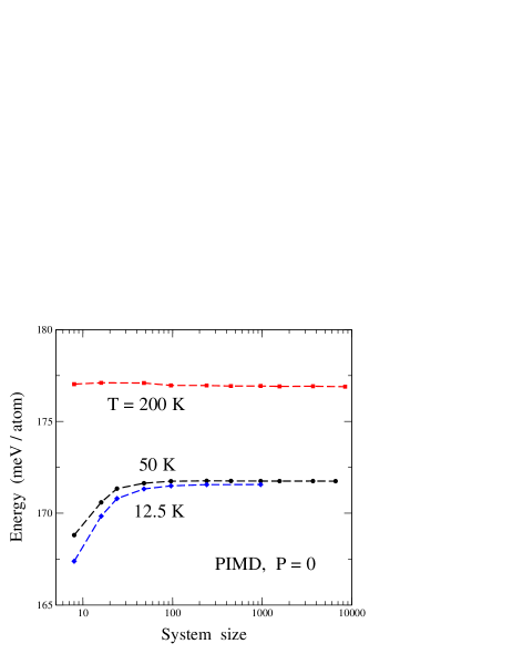
Figure 1: Internal energy per atom vs system size, as derived from PIMD simulations at $P$ = 0. From top to bottom: $T$ = 200, 50, and 12.5 K. Dashed lines are guides to the eye. Error bars are less than the symbol size.

In our simulations of graphene, both kinetic and potential energy were found to slightly increase with system size, but their convergence is rather fast. In Fig. 1 we present the internal energy per atom derived from PIMD simulations as a function of cell size at three temperatures: 200 K (squares), 50 K (circles), and 12.5 K (diamonds). At the lowest temperature, there appears a shift of about 4 meV/atom when increasing the cell size from 8 atoms to the largest sizes considered here. For cells in the order of 200 atoms the size effect in the internal energy is almost inappreciable when compared to the largest cells. The potential energy was found earlier to be smaller than the kinetic energy, indicating a nonnegligible anharmonicity of the lattice vibrations.Herrero and Ramírez (2016) The convergence with system size becomes faster as the temperature is raised. This is basically due to the fact that increasing the cell size effectively causes the appearance of low vibrational frequencies in the system, that do not appear for smaller sizes. Increasing the temperature makes that these new low-frequency modes behave “more classically” (see Sec. V.A below).

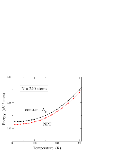
Figure 2: Internal energy obtained from PIMD simulations in the $NPT$ ensemble ($P=0$) (circles) and in the constant-$A_{p}$ ensemble with $A_{p}=A_{0}$ (squares). Note the zero-point energy, which amounts to about 0.17 eV/atom. Error bars of the simulation data are smaller than the symbol size.

In Fig. 2 we display the temperature dependence of the internal energy, as derived from PIMD in the $NPT$ isothermal-isobaric ensemble, for system size $N$ = 240. For comparison, we also present results obtained from constant-$A_{p}$ simulations with fixed area $A_{p}=A_{0}$. The zero-point energy, $E_{\rm ZP}$, is found to be close to 0.17 eV/atom in both cases. In the isobaric simulations, however, $E_{\rm ZP}$ is somewhat lower than in the fixed-$A_{p}$ simulations, mainly due to the zero-point expansion of the graphene layer with respect to the classical minimum $A_{0}$. This expansion relaxes the compressive stress appearing for area $A_{0}$ in the presence of atomic quantum motion, and consequently the energy decreases. The difference between zero-point energy in both cases amounts to 1 meV/atom. This difference between both sets of results decreases for rising temperature, and eventually the constant-area energy becomes lower than the $P=0$ result for $T\gtrsim$ 1000 K (not shown in the figure).

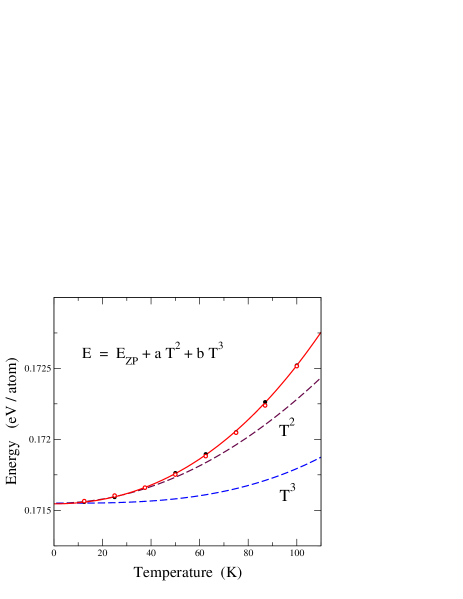
Figure 3: Temperature dependence of the internal energy of graphene in the region up to 100 K. Symbols represent simulation results for $P=0$ obtained for $N=240$ (solid circles) and $N=960$ (open circles). The line is a fit of the data points to the expression $E=E_{\rm ZP}+aT^{2}+bT^{3}$, with $E_{\rm ZP}$ the zero-point energy. The dashed lines represent the contributions of the $T^{2}$ and $T^{3}$ terms to the fitted curve.

To better appreciate the low-temperature region, we present in Fig. 3 the temperature dependence of the internal energy obtained from PIMD simulations in the $NPT$ ensemble up to $T\sim$ 100 K. Symbols indicate results of the simulations for $N=240$ (solid circles) and $N=960$ (open circles). Note that several solid circles are nearly unobservable, as they lie under the results for 960 atoms. The solid line is a fit to the expression $E=E_{\rm ZP}+aT^{2}+bT^{3}$, which displays a good agreement with a temperature dependence of the energy in the region shown in Fig. 3. For the coefficients $a$ and $b$ we found: $a=7.1\times 10^{-8}$ eV K^-2 and $b=2.7\times 10^{-10}$ eV K^-3. Note that a linear term in this expression for the internal energy is not possible for thermodynamic consistency, since the specific heat $c_{p}=(\partial E/\partial T)_{P}$ has to vanish for $T\to 0$. In Fig. 3 we also present separately the contributions of the $T^{2}$ and $T^{3}$ terms (dashed lines). The $T^{2}$ term is the main contribution to the energy in the considered region, and controls the temperature dependence of the energy up to about 40 K. This is important for the low-temperature specific heat and will be further discussed in Sec. V.

IV Structural properties

In our simulations in the isothermal-isobaric ensemble one fixes the applied stress in the $(x,y)$ plane (here $P=0$), allowing changes in the in-plane area of the simulation cell for which periodic boundary conditions are applied. Carbon atoms are free to move in the out-of-plane direction ($z$ coordinate), and in general any measure of the “real” surface of a graphene sheet at $T>0$ should give a value larger than the area of the simulation cell in the $(x,y)$ plane. In this line, it has been argued for biological membranes that their properties should be described using the concept of a real surface instead of a “projected” (in-plane) surface.Imparato (2006); Waheed and Edholm (2009); Chacón et al. (2015) A similar question can be risen for crystalline membranes such as graphene. This may be relevant for calculating thermodynamic properties, since the in-plane area $A_{p}$ is the variable conjugate to the stress $P$ used in our simulations, and the real area (also called true, effective, or actual area in the literatureImparato (2006); Fournier and Barbetta (2008); Waheed and Edholm (2009); Chacón et al. (2015)) is conjugate to the usually-called surface tension.Safran (1994) It is, in fact, the in-plane area $A_{p}$ which has been commonly employed in the literature to describe the results of atomistic simulations of graphene layers.Gao and Huang (2014); Brito et al. (2015); Zakharchenko et al. (2009); Los et al. (2016); Chacón et al. (2015) In the framework of biological membranes, it was shown that values of the compressibility may be very different when they are related to $A$ or to $A_{p}$, and something similar has been recently found for the elastic properties of graphene.Ramírez and Herrero (2017)

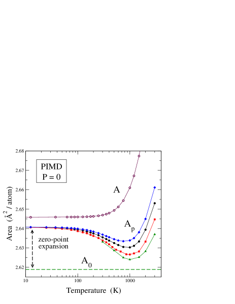
Figure 4: In-plane and real area vs temperature. Solid symbols represent results for the in-plane area $A_{p}$, as derived from isothermal-isobaric PIMD simulations for several system sizes. From top to bottom, $N$ = 96 (diamonds), 240 (circles), 960 (squares), and 33600 (triangles). Open circles correspond to the real area $A$ obtained for $N$ = 240 atoms; other system sizes yielded results for $A$ indistinguishable from those presented here. Solid lines are guides to the eye. Error bars are less than the symbol size. The dashed line indicates the minimum-energy area $A_{0}$.

Here we calculate a real area $A$ in 3D space by a triangulation based on the actual atomic positions. Each structural hexagon contributes to the area $A$ by a sum of six triangles, each one formed by the positions of two adjacent C atoms and the centroid (barycenter) of the hexagon (mean position of the corresponding six vertices).Ramírez and Herrero (2017) Other, qualitatively similar, definitions can be used for the real area, such as those based on the interatomic distance C–C.Hahn et al. (2016); Herrero and Ramírez (2016) In Fig. 4 we show the temperature dependence of the in-plane area $A_{p}$ and the real area $A$ of graphene, as derived from PIMD simulations, in a semilogarithmic plot. For $A_{p}$ we present results for various cell sizes as solid symbols. From top to bottom: $N$ = 96 (diamonds), 240 (circles), 960 (squares), and 33600 (triangles). Open circles represent results for the area $A$ obtained with $N$ = 240 atoms; results for larger cells are indistinguishable from them. In fact, $A$ shows, in contrast to $A_{p}$, a small finite-size effect not visible at the scale of Fig. 4. The horizontal dashed line in Fig. 4 indicates the minimum-energy area $A_{0}$, corresponding to a planar classical sheet at $T=0$.

For the area $A$ one observes a nearly constant value up to about 200 K, followed by an increase at higher temperatures, similar to that observed for the volume of 3D crystalline solids such as diamond.Herrero and Ramírez (2000) The in-plane area $A_{p}$ decreases in the range from $T=0$ to temperatures in the order of 1000 K, where it reaches a minimum, and then it increases at higher $T$. Here, the finite-size effect is important in both the temperature $T_{m}$ of the minimum and the value of the minimum area. For rising system size, the temperature $T_{m}$ shifts to higher values, whereas the minimum $A_{p}$ decreases with increasing $N$. These results for the in-plane area are reminiscent of those found from classical Monte Carlo and molecular dynamics simulations of graphene,Zakharchenko et al. (2009); Gao and Huang (2014); Brito et al. (2015) but in PIMD simulations we find a more pronounced decrease in $A_{p}$ in the temperature region from 0 to 1000 K.

In the limit $T\to 0$, the areas $A$ and $A_{p}$ converge to 2.6459 Ų and 2.6407 Ų, respectively. It is important to note that, in spite of the appreciable differences in the in-plane area per atom for the different system sizes, all of them converge at low $T$ to the same value. In the low-temperature region one observes first a zero-point expansion of about 0.02 Ų ($\sim$ 1%), mainly due to an increase in the mean C–C bond length, caused by zero-point vibrations (an anharmonic effect). The small difference of a 0.2% between real and in-plane areas is associated to out-of-plane zero-point motion, which causes that even at $T=0$ the layer is not strictly planar. Note that this is a pure quantum effect, since in classical simulations at $T\to 0$ one finds a planar layer in which $A$ and $A_{p}$ coincide.Herrero and Ramírez (2016); Ramírez and Herrero (2017)

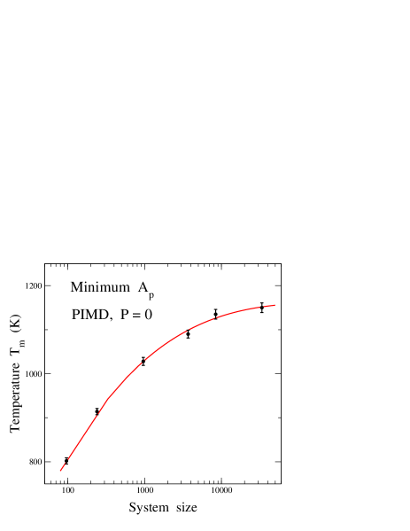
Figure 5: Temperature $T_{m}$ corresponding to the minimum in-plane area $A_{p}$ vs system size $N$, as derived from PIMD simulations for $P=0$. The line is a polynomial fit the the data points.

Moreover, the temperature $T_{m}$ at which $A_{p}$ reaches its minimum is size-dependent (see Fig. 4). In Fig. 5 we present the dependence of $T_{m}$ on system size. Solid symbols indicate results of PIMD, and the solid line is a polynomial fit to the data points. It has been shown earlier from extensive classical simulations that the in-plane area $A_{p}$ has an important finite-size effect, but its large-$N$ limit is well defined.Ramírez et al. (2016); Los et al. (2016) Something similar is expected for the results of PIMD simulations, and in particular for the temperature $T_{m}$. Thus, in the large-$N$ limit, the size-dependent $T_{m}$ converges to a value $\lesssim$ 1200 K. A more precise result for this limit would require consideration of larger system sizes, not accessible at present with our simulation procedure.

Beginning from $T=0$, the surface $A$ is larger than $A_{p}$, and the difference between both increases with temperature. In fact, $A_{p}$ is the projection of $A$ on the $(x,y)$ plane, and the actual surface becomes increasingly bent as temperature is raised and out-of-plane atomic displacements are larger. For the area $A$ we do not observe the decrease displayed by $A_{p}$. Moreover, the areas $A$ and $A_{p}$ derived from PIMD simulations show a temperature derivative which approaches zero as $T\to 0$, in agreement with the third law of thermodynamics.

The behavior of $A_{p}$ as a function of $T$ is basically due to a competition between two opposite factors. First, the real area $A$ rises as $T$ is increased in the whole temperature range considered here. Second, bending of the surface gives rise to a decrease in its 2D projection, $A_{p}$. At $T\lesssim$ 1000 K, the decrease due to out-of-plane vibrations dominates the thermal expansion of the real surface, so that $dA_{p}/dT<0$. At $T\gtrsim$ 1000 K, the increase in $A$ dominates the contraction in the projected area associated to out-of-plane atomic displacements. This behavior is qualitatively similar to that found from classical molecular dynamics and Monte Carlo simulations, as well as analytical calculations, where a minimum in the temperature dependence of $A_{p}$ was also found.Zakharchenko et al. (2009); Gao and Huang (2014); Michel et al. (2015); Herrero and Ramírez (2016) The main difference is that the contraction of $A_{p}$ respect the zero-temperature value is in the quantum case significantly larger than for classical calculations.

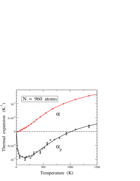
Figure 6: Thermal expansion coefficients $\alpha$ and $\alpha_{p}$ of graphene vs temperature, as derived from PIMD simulations for a cell including 960 atoms. Symbols are data points obtained from numerical derivatives of $A$ and $A_{p}$ (squares, $\alpha$; circles, $\alpha_{p}$). Solid lines indicate the temperature derivatives of polynomial fits to the obtained values for $A$ and $A_{p}$. Error bars for $\alpha$ are less than the symbol size.

According to our definitions of the areas $A$ and $A_{p}$, we consider two different thermal expansion coefficients:

$$\alpha=\frac{1}{A}\left(\frac{\partial A}{\partial T}\right)_{P}$$ (1)

and

$$\alpha_{p}=\frac{1}{A_{p}}\left(\frac{\partial A_{p}}{\partial T}\right)_{P}\,.$$ (2)

The area $A$ derived from our PIMD simulations shows a negligible size effect for $N\gtrsim$ 100 atoms, as indicated above. Hence, the same occurs for the coefficient $\alpha$, which vanishes in the zero-temperature limit and turns out to be positive at all finite temperatures considered here. In Fig. 6 we display the thermal expansion coefficients $\alpha$ and $\alpha_{p}$ derived from our simulations. Symbols are data points obtained from a numerical derivative of the areas $A$ (squares) and $A_{p}$ (circles) corresponding to $N$ = 960. For these derivatives we took temperature intervals ranging from 10 K at low temperature to about 100 K at temperatures higher than 1000 K. To check the precision of these numerical derivatives, we fitted the obtained values for $A$ and $A_{p}$ to polynomial expressions in the temperature range from $T$ = 10 to 1500 K. We then obtained the temperature derivative of these polynomials, which yielded the solid lines displayed in Fig. 6. The agreement between both procedures for calculating $\alpha$ and $\alpha_{p}$ is good. Note that the noise in the values of $\alpha_{p}$ obtained from numerical differences is clearly larger than that found for $\alpha$, as a consequence of the larger fluctuations in $A_{p}$.

Both $\alpha$ and $\alpha_{p}$ converge to zero in the low-temperature limit. The behavior of $\alpha$ is similar to that observed for crystalline materials, as indicated above for the temperature dependence of the area $A$. However, $\alpha_{p}$ decreases fast for increasing temperature, until reaching a minimum, which for $N=960$ amounts to $\approx-9\times 10^{-6}$ K^-1 at $T_{m}\sim$ 200 K. At higher $T$, $\alpha_{p}$ rises and becomes positive at a temperature of about 1000 K (where $A_{p}$ reaches its minimum value). In view of the results for $A_{p}$ displayed in Fig. 4, the minimum value of $\alpha_{p}$ is expected to be size-dependent. Analyzing the results for the different system sizes studied here, we estimate in the large-size limit a minimum value $\alpha_{p}=-1.1(\pm 0.1)\times 10^{-5}$ K^-1. It is interesting to note that the difference $\alpha-\alpha_{p}$, which vanishes at $T=0$, increases fast as temperature is raised, and takes a value $\approx 10^{-5}$ K^-1 for temperatures higher than 1000 K.

Our results for $\alpha_{p}$ are qualitatively similar to those derived earlier from other theoretical techniques. Jiang et al.Jiang et al. (2009) employed a nonequilibrium Green’s function approach, and found for free-standing graphene a minimum $\approx 10^{-5}$ K^-1, close to our data shown in Fig. 6. They found a crossover from negative to positive $\alpha_{p}$ at a temperature $T\approx$ 600 K, lower than our PIMD results. Such a crossover at a point with $\alpha_{p}=0$ was obtained by da Silva et al.da Silva et al. (2014) at $T\approx$ 400 K from an unsymmetrized self-consistent-field method. Experimental results at room temperature are not far from our data at 300 K: $\alpha_{p}=-8\times 10^{-6}$ K^-1 derived from Raman spectroscopy results,Yoon et al. (2011) and $-7\times 10^{-6}$ K^-1 found from scanning electron microscopy.Bao et al. (2009) The consistency between different measurements is not so good for the temperature dependence of $\alpha_{p}$, and in fact the increase in $\alpha_{p}$ at $T>$ 300 K is much faster in the former case Yoon et al. (2011) than it the latter.Bao et al. (2009)

To make connection of our results derived from atomistic simulations with analytical formulations of membranes, we note that the relation between $A$ and $A_{p}$ can be expressed in the continuum limit (macroscopic view) asImparato (2006); Waheed and Edholm (2009); Ramírez and Herrero (2017)

$$A=\int_{A_{p}}dx\,dy\,\sqrt{1+(\nabla h(x,y))^{2}}\;,$$ (3)

where $h(x,y)$ is the height of the membrane surface, i.e. the distance to the reference $(x,y)$ plane. The difference between the expansion coefficients $\alpha$ and $\alpha_{p}$ at high temperature can be understood from the relation between real and projected areas, $A$ and $A_{p}$, given by this equation.

In fact, the difference $A-A_{p}$ for a continuous membrane in a classical approach may be calculated by Fourier transformation of the r.h.s. of Eq. (3).Safran (1994); Chacón et al. (2015); Ramírez and Herrero (2017) This requires the introduction of a dispersion relation $\omega({\bf k})$ for out-of-plane modes (ZA band), where ${\bf k}=(k_{x},k_{y})$ are 2D wavevectors. The frequency dispersion in this acoustic (flexural) band can be well approximated by the expression $\rho\,\omega^{2}=\sigma k^{2}+\kappa k^{4}$, consistent with an atomic description of grapheneRamírez et al. (2016) ($k=|{\bf k}|$; $\rho$, surface mass density; $\sigma$, effective stress; $\kappa$, bending modulus). Thus, one findsRamírez and Herrero (2017)

$$A=A_{p}\left(1+\frac{k_{B}T}{4\pi}\int_{0}^{k_{m}}dk\frac{k}{\sigma+\kappa k^{2}}\right)\,,$$ (4)

with the wavevector cut-off $k_{m}=(2\pi/A_{p})^{1/2}$.

For effective stress $\sigma>0$, which is the case at finite temperatures, even for zero external stress ($P=0$),Ramírez et al. (2016); Ramírez and Herrero (2017) the integral in Eq. (4) converges, yielding

$$A=A_{p}\left[1+\frac{k_{B}T}{8\pi\kappa}\ln\left(1+\frac{2\pi\kappa}{\sigma A_{p}}\right)\right]\>.$$ (5)

Note that this expression has been derived in the classical limit, i.e., without taking into account atomic quantum delocalization. It is expected, however, to be a good approximation to our quantum calculations at relatively high temperature, $T\gtrsim\Theta_{D}$, with $\Theta_{D}\sim$ 1000 K the Debye temperature associated to out-of-plane vibrations in graphene.Tewary and Yang (2009); Politano et al. (2011)

It is not straightforward to write down an analytical expression for $\alpha-\alpha_{p}$ from a temperature derivative of Eq. (5), as one has to include changes in $\kappa$ and $\sigma$ through $\partial\kappa/\partial T$ and $\partial\sigma/\partial T$. One can instead obtain the temperature dependence of these parameters from a fit to earlier results of classical simulations.Ramírez et al. (2016) Thus, we obtain from Eq. (5) at $T$ = 1000 K a difference $\alpha-\alpha_{p}=8.5\times 10^{-6}$ K^-1, close to the high-temperature results obtained from our PIMD simulations ($\sim 10^{-5}$ K^-1).

Our low-temperature data for $A_{p}(T)$ and the trend $\alpha_{p}\to 0$ in the low-temperature limit are consistent with the results obtained by Amorim et al.,Amorim et al. (2014) from first-order perturbation theory and a one-loop self-consistent approximation. These authors emphasized that the limits $N\to\infty$ and $T\to 0$ do commute, which agrees with the results of our simulations, i.e., at low $T$ all system sizes yield the same results. In general, the evaluation of low-temperature properties from PIMD simulations becomes increasingly harder for both, larger $N$ and lower $T$. In the case of graphene, this is complicated by the fact that larger sizes may require lower temperatures to converge to the ground-state properties, as shown for the area $A_{p}$ in Fig. 4.

V Specific heat

V.1 Harmonic approximation

For comparison with the results of our PIMD simulations for the specific heat of graphene, we will discuss here a harmonic approximation (HA) for the lattice vibrations. Even though this approximation will turn out to be rather accurate at low temperatures, it is clear that anharmonicity will show up as temperature is raised, and the results of this approximation will progressively depart from those more realistic derived from the simulations. The HA assumes constant frequencies for the graphene vibrations (those derived for the minimum-energy configuration), and does not take into account changes of the areas $A$ and $A_{p}$ with temperature. For solids, volume changes are usually considered through quasi-harmonic approximations, which take into account the thermal expansion and its corresponding changes in vibrational frequencies (usually by means of Grüneisen constantsAshcroft and Mermin (1976); Mounet and Marzari (2005); Ramírez et al. (2012)). The same procedure is not directly applicable for graphene at any temperature, as due to the compression of $A_{p}$ the crystalline membrane becomes unstable in a quasi-harmonic approximation for $A_{p}<A_{0}$ with the appearance of imaginary frequencies when diagonalizing the dynamical matrix. This can be remedied at low temperatures for finite-size graphene layers, but the whole scheme becomes unstable at relatively high $T$, or yields unphysical results, as a continuous contraction of graphene at any temperature,Mounet and Marzari (2005) in disagreement with results of both classical and PIMD simulations.Zakharchenko et al. (2009); Michel et al. (2015); Los et al. (2016); Gao and Huang (2014); Herrero and Ramírez (2016)

For a simulation cell including $N$ atoms, the specific heat per atom, $c_{v}(T)=dE(T)/dT$, is given in the HA by

$$c_{v}(T)=\frac{k_{B}}{N}\sum_{r,\bf k}\frac{\left[\frac{1}{2}\beta\hbar\,\omega_{r}({\bf k})\right]^{2}}{\sinh^{2}\left[\frac{1}{2}\beta\hbar\,\omega_{r}({\bf k})\right]}\,,$$ (6)

where $\beta=1/(k_{B}T)$, and the index $r$ ($r$ = 1, …, 6) refers to the six phonon bands of graphene (ZA, ZO, LA, TA, LO, and TO).Mounet and Marzari (2005); Karssemeijer and Fasolino (2011); Wirtz and Rubio (2004) The sum in ${\bf k}$ is extended to wavevectors ${\bf k}=(k_{x},k_{y})$ in the hexagonal Brillouin zone, with discrete ${\bf k}$ points spaced by $\Delta k_{x}=2\pi/L_{x}$ and $\Delta k_{y}=2\pi/L_{y}$.Ramírez et al. (2016) Eq. (6) has been used to calculate the specific heat presented below. Increasing the system size $N$ causes the appearance of vibrational modes with longer wavelength $\lambda$. In fact, one has for the phonons an effective cut-off $\lambda_{max}\approx L$, with $L=(NA_{p})^{1/2}$, and the minimum wavevector is $k_{0}=2\pi/\lambda_{max}$, i.e., $k_{0}\sim N^{-1/2}$.

The low-temperature behavior of the heat capacity vs $T$ can be further analyzed by considering a continuous model for frequencies and wavevectors, similarly to the well-known Debye model for solids.Ashcroft and Mermin (1976); Kittel (1966) At low-temperatures, $c_{v}$ is dominated by the contribution of acoustic modes with small $k$. For graphene, these are TA and LA modes with $\omega_{r}\propto k$ and ZA modes with $\omega_{r}\propto k^{2}$ ($\sigma$ is negligible at low $T$ and zero external stress).

The low-$T$ contribution of a phonon branch with dispersion relation $\omega_{r}\propto k^{n}$ can be approximated as

$$c_{v}^{r}(T)\approx k_{B}\int_{k_{0}}^{k_{m}}\frac{\left[\frac{1}{2}\beta\hbar\,\omega_{r}(k)\right]^{2}}{\sinh^{2}\left[\frac{1}{2}\beta\hbar\,\omega_{r}(k)\right]}\,\rho(k)\,dk\,,$$ (7)

where $k_{m}$ is the maximum wavenumber $k_{m}=(2\pi/A_{0})^{1/2}$ and $\rho(k)=A_{0}k/2\pi$ for 2D systems. From the dispersion relation $\omega_{r}(k)$, we have a vibrational density of states $\bar{\rho}_{r}(\omega)\sim\omega^{\frac{2}{n}-1}$ Introducing the large-size limit $\omega_{0}\to 0$ and putting $x=\frac{1}{2}\beta\hbar\,\omega$, one finds

$$c_{v}^{r}\sim k_{B}\frac{K}{(\beta\hbar)^{\frac{2}{n}}}\int_{0}^{x_{m}}\frac{x^{\frac{2}{n}+1}}{\sinh^{2}x}\,dx\,,$$ (8)

$K$ being a constant. Then, for low temperatures, $k_{B}T\ll\hbar\,\omega_{m}$, one has $c_{v}^{r}\sim T^{2/n}$. In general, for $d$-dimensional systems one finds an exponent $d/n$.Hone (2001); Popov (2002) Thus, for the ZA phonon branch in graphene ($n=2$), one expects a linear dependence of $c_{v}^{r}$ on $T$, whereas for the contribution of LA and TA branches ($n=1$), one has at low temperature $c_{v}^{r}\sim T^{2}$. Putting all constants in the integrals, we find for the ZA branch

$$c_{v}^{ZA}=\frac{\pi}{12}\frac{k_{B}^{2}}{\hbar}\sqrt{\frac{\rho}{\kappa}}A_{0}\,T\,,$$ (9)

and for acoustic LA and TA modes:

$$c_{v}^{ac}=\frac{3\zeta(3)}{\pi}\frac{k_{B}^{3}}{\hbar^{2}}\frac{A_{0}}{v^{2}}\,T^{2}\,,$$ (10)

$v$ being the sound velocity in the corresponding phonon branch, and $\zeta$ is the Riemann zeta function.

For in-plane vibrations of graphene, the acoustic branches can be described by the linear dispersion $\omega_{i}=v_{i}k$, with sound speed $v_{1}$ = 21.5 km/s for LA and $v_{2}$ = 14.0 km/s for TA modes. These values for $v_{1}$ and $v_{2}$ were derived from the elastic properties of graphene obtained by using the LCBOPII potential,Ramírez and Herrero (2017) and are close to those given by Karssemeijer and Fasolino,Karssemeijer and Fasolino (2011) as well as to those derived from ab-initio calculations for grapheneMounet and Marzari (2005) and experimental data for graphite.Wirtz and Rubio (2004) For the bending constant $\kappa$ describing the ZA phonon band, we take $\kappa$ = 1.49 eV.Ramírez et al. (2016)

V.2 Elastic energy

Apart from the pure vibrational energy associated to the phonons in graphene, one has even in the presence of an externally applied stress, an elastic energy due to changes in the area $A$ of the crystalline membrane (thermal expansion). Thus, the internal energy $E(T)$ at temperature $T$ can be written asHerrero and Ramírez (2016)

$$E(T)=E_{0}+E_{\rm el}(A)+E_{\rm vib}(A,T)\,,$$ (11)

where $E_{\rm el}(A)$ is the elastic energy corresponding to an area $A$, and $E_{\rm vib}(A,T)$ is the vibrational energy of the system. Our PIMD simulations directly give $E(T)$, which can be split into an elastic and a vibrational part.

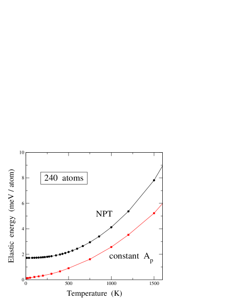
Figure 7: Elastic energy of graphene, $E_{\rm el}$, as derived from the real area obtained in PIMD simulations in the $NPT$ ensemble for $P=0$ (circles) and in the constant-$A_{p}$ ensemble with the in-plane area corresponding to the minimum energy, $A_{p}=A_{0}$ (squares). Lines are guides to the eye.

The elastic energy $E_{\rm el}$ corresponding to an area $A$ is defined here as the increase in energy of a strictly planar graphene layer with respect to the minimum energy $E_{0}$. We have calculated $E_{\rm el}(A)$ for a supercell including 960 atoms, expanding it isotropically and keeping it flat. As indicated above for the area $A$, finite-size effects on the elastic energy are very small, and in practice negligible for our current purposes. The elastic energy $E_{\rm el}(A)$ increases with $A$, and for small lattice expansion it can be approximated as $E_{\rm el}(A)\approx K(A-A_{0})^{2}$, with $K$ = 2.41 eV/Ų. The elastic energy turns out to be much smaller than the vibrational energy in the cases considered here, but it can be nonnegligible for the actual heat capacity of graphene, as the area $A$ changes with temperature.

In Fig. 7 we present the elastic energy $E_{\rm el}$ as a function of temperature for our $NPT$ simulations at $P=0$. For comparison we also show results derived from constant-$A_{p}$ simulations with the minimum-energy area $A_{0}$. $E_{\rm el}$ is found to increase with $T$ in both cases, but there are some differences between them. In the isothermal-isobaric simulations (circles) we find an appreciable elastic energy in the zero-temperature limit, basically due to zero-point lattice expansion (see Sec. IV). In the constant-$A_{p}$ simulations (squares) such an expansion is not allowed, and $E_{\rm el}$ is nearly zero; a small positive value of $E_{\rm el}$ is obtained for $T\to 0$, caused by a slight increase in the area $A$ due to out-of-plane zero-point vibrations. The difference between elastic energy in both kinds of simulations decreases from $T$ = 0 until about 1000 K, and then it increases at higher temperatures. This is related to the dependence of the in-plane area in $NPT$ simulations upon temperature, which approaches the area $A_{0}$ up to 1000 K, and departs from it at higher $T$ (see Fig. 4).

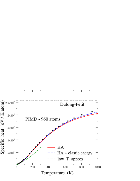
Figure 8: Specific heat of graphene as a function of temperature. Symbols represent results for $c_{p}$ derived from PIMD simulations for $N$ = 960 atoms. Error bars of the data points are less than the symbol size. The solid line is $c_{v}$ obtained from the six phonon bands corresponding to the LCBOPII potential in a harmonic approximation. The dashed line includes the contribution $dE_{\rm el}/dT$ of the elastic energy. The horizontal dashed-dotted line represents the harmonic classical limit (Dulong-Petit law).

V.3 Comparison with PIMD simulations

We now turn to the results of our simulations. In Fig. 8 we show the specific heat of graphene as a function of temperature. Solid circles represent results for $c_{p}$, derived from PIMD simulations for $N$ = 960 atoms. They were obtained from a numerical derivative of the internal energy $E(T)$. Results corresponding to $N$ = 240 are indistinguishable from those plotted in Fig. 8. The solid line was calculated with the HA using Eq. (6), with the frequencies $\omega_{r}({\bf k})$ ($r$ = 1, …, 6) obtained from diagonalization of the dynamical matrix corresponding to the LCBOPII potential.Karssemeijer and Fasolino (2011) Results of the simulations follow closely the HA up to about 400 K, and they become progressively higher than the solid line for higher temperatures, at which anharmonic effects are expected to increase.

As indicated above, a part of the internal energy at a given temperature corresponds to the elastic energy $E_{\rm el}$, i.e. to the cost of increasing the area $A$ of graphene. We have calculated the contribution of this energy to the specific heat as $dE_{\rm el}/dT$, using the data obtained from PIMD simulations in the $NPT$ ensemble, shown in Fig. 7. To assess the importance of this contribution to the whole specific heat, we have added it to the result of the HA (solid line in Fig. 8), and have displayed the sum as a dashed line. We find an observable increase in the specific heat respect the pure HA, especially visible for $T>500$ K, such that it incorporates part of the anharmonicity of the system, yielding a result closer to the specific heat $c_{p}$ derived from the simulations. For comparison, the classical Dulong-Petit specific heat is shown as a dashed-dotted line ($c_{v}^{cl}=3k_{B}$). At $T$ = 1000 K the quantum results are still appreciably lower than the classical limit.

We have also calculated the specific heat $c_{v}$ from constant-$A_{p}$ simulations. For each temperature, we take the equilibrium area $A_{p}$ obtained in the $NPT$ simulations, and calculate $c_{v}$ as $\Delta E/\Delta T$ for that value of $A_{p}$ from increments $\Delta T$ (both positive and negative). Note that this is not the same as taking a temperature derivative of the energy curve shown in Fig. 1 for the constant-$A_{p}$ ensemble, since in this case the simulations were carried out with minimum-energy area $A_{0}$. It is expected that $c_{v}\leq c_{p}$ at any temperature, but the difference between them turns out to be smaller than the statistical error bar of our results, so that they appear as indistinguishable from the direct results of our PIMD simulations (see below).

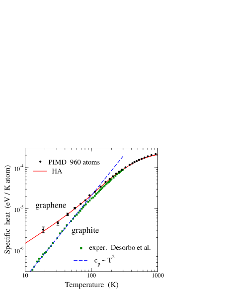
Figure 9: Specific heat of graphene as a function of temperature. Solid circles represent results for $c_{p}$ derived from PIMD simulations for $N$ = 960 atoms. The solid line was obtained from the six phonon bands corresponding to the LCBOPII potential in a harmonic approximation. For comparison, experimental data for graphite obtained by Desorbo and TylerDesorbo and Tyler (1953) are shown as squares. The dashed line displays a dependence $c_{p}\sim T^{2}$.

An analytical expression for $c_{v}(T)$ at low temperature can be derived in the HA from the contribution $c_{v}^{r}$ of modes ZA, LA, and TA, as given by Eqs. (9) and (10). The sum of contributions of these three phonon bands is plotted in Fig. 8 as a dashed-dotted line. It follows the simulation data and the whole HA up to $T\sim$ 50 K, and at high temperatures it becomes lower.

To display more clearly the low-temperature region, we present in Fig. 9 the specific heat vs temperature in a semilogarithmic plot. Solid circles are results for $c_{p}$ derived from PIMD simulations for $N$ = 960. The solid line indicates the harmonic approximation for $c_{v}$ obtained from Eq. (6) for the same cell size. At low temperature, it is clear the linear dependence of the specific heat on $T$ (slope unity in the logarithmic plot). In fact we find at low temperature $c_{p}\approx CT$ with $C=1.4\times 10^{-7}$ eV K^-2 (Note that $C=2a$, with $a$ the coefficient of the quadratic term in the fit of the energy shown in Fig. 3). For comparison we also present in Fig. 9 experimental data for $c_{p}$ of graphite, obtained by Desorbo and Tyler.Desorbo and Tyler (1953) The temperature dependence of the heat capacity of graphite has been studied in detail along the years.Komatsu and Nagamiya (1951); Krumhansl and Brooks (1953); Klemens (1953); Nicklow et al. (1972) In this case, $c_{p}$ rises as $T^{3}$ for $T<$ 10 K (a region not reached here and not shown in Fig. 9). At temperatures between 10 and 100 K, $c_{p}$ increases as $T^{2}$. The main difference with graphene is that the dominant contribution to $c_{p}$ in this temperature region comes from phonons with a linear dispersion relation ($\omega\sim k$) for small $k$. At room temperature the specific heat of graphite amounts to $8.90\times 10^{-5}$ eV / K atom, i.e. 8.59 J / K mol, somewhat smaller than our results of PIMD simulations for graphene: $c_{p}=9.4(\pm 0.1)\times 10^{-5}$ eV / K atom.

The difference between $c_{p}$ and $c_{v}$ has been obtained from the thermodynamic relation

$$c_{p}-c_{v}=T\alpha_{p}^{2}B_{p}A_{p}\,$$ (12)

where $B_{p}$ is the in-plane isothermal bulk modulus, i.e. $B_{p}=-A_{p}\,(\partial P/\partial A_{p})_{T}$. Eq. (12) is similar to the relation between $c_{p}$ and $c_{v}$ for 3D systems.Callen (1960); Landau and Lifshitz (1980) Note that the variables appearing on the r.h.s. of Eq. (12) refer to in-plane properties, as the pressure appearing in our $NPT$ ensemble is the conjugate variable of the in-plane area $A_{p}$. $B_{p}$ has been calculated by using the fluctuation formula:Landau and Lifshitz (1980); Ramírez and Herrero (2017)

$$B_{p}=\frac{k_{B}TA_{p}}{N(\Delta A_{p})^{2}}$$ (13)

with $(\Delta A_{p})^{2}$ the mean-square fluctuations of the in-plane area $A_{p}$ obtained in the simulations. This expression is more convenient for our purposes than obtaining $(\partial A_{p}/\partial P)_{T}$, as this derivative requires additional simulations at nonzero stresses. In any case, we have checked at some selected temperatures that both procedures yield the same results for $B_{p}$ (taking into account the error bars).

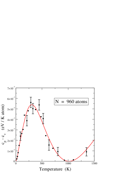
Figure 10: Difference $c_{p}-c_{v}$ vs temperature, as obtained from the thermodynamic expression $c_{p}-c_{v}=T\alpha_{p}^{2}B_{p}A_{p}$. Symbols were derived from the values of $\alpha_{p}$, $B_{p}$, and $A_{p}$ directly derived from PIMD simulations, whereas the solid line was calculated from polynomial fits of these quantities as a function of temperature.

Thus, we have obtained the difference $c_{p}-c_{v}$ introducing into Eq. (12) the values of $\alpha_{p}$, $B_{p}$, and $A_{p}$ derived from PIMD simulations. The results are shown in Fig. 10 as a function of temperature (solid circles). The solid line in this figure was obtained by using Eq. (12) and polynomial fits for the temperature dependence of the factors in the r.h.s. of this equation. In the zero-temperature limit the difference $c_{p}-c_{v}$ converges to zero, as should happen because both specific heats vanish as $T\to 0$, and this difference increases for rising temperature until $T\sim$ 300 K, where it reaches a maximum of $\approx 5.5\times 10^{-7}$ eV/(K atom). At higher $T$, $c_{p}-c_{v}$ decreases and reaches zero at the temperature at which $\alpha_{p}$ vanishes ($\sim$ 1000 K). Note that the vanishing of the difference $c_{p}-c_{v}$ at a finite temperature (here $T\sim$ 300 K) obtained for graphene is similar to that occurring for some 3D materials with negative thermal expansion at low $T$ (e.g., crystalline silicon),Shah and Straumanis (1972); Evans (1999) according to the thermodynamic equation $c_{p}-c_{v}=T\alpha^{2}BV$.

We emphasize here that the calculation of the low-temperature specific heat of materials using path-integral simulations is not in general an easy task. In fact, even the reproduction of the Debye law $c_{p}\sim T^{3}$ for 3D solids has been a challenge for PIMD of solids, due to the effective low-frequency cut-off associated to finite simulation cells.Noya et al. (1996); Ramírez et al. (2006) The reliability of this kind of calculations for 2D materials such as graphene is mainly due to two reasons. First, the length of the cell sides scales as $L\sim N^{1/d}$, so that the minimum wavevector accessible in the simulation is $k_{0}\sim N^{-1/d}$. Then, for a simulation cell including $N$ atoms, $k_{0}$ is smaller for 2D than for 3D materials, which means that the low-frequency region is better described in the former case, and consequently also the low-temperature regime. Second, and even more important, is the fact that the internal energy for graphene rises as $T^{2}$ (or $c_{p}\sim T$), which is a fast increase, much easily detectable than the typical expectancy ($E\sim T^{4}$) for the phonon contribution in 3D materials ($c_{p}\sim T^{3}$).

We note that the electronic contribution to the specific heat of graphene has not been taken into account for the temperatures considered here, as it is much less than the phonon contribution. The former has been estimated in several works, and turns out to be between three and four orders of magnitude smaller than the latter in pure graphene.Benedict et al. (1996); Nihira and Iwata (2003); Fong et al. (2013)

A thermodynamic parameter related to the thermal expansion and specific heat is the dimensionless Grüneisen parameter $\gamma$,Ashcroft and Mermin (1976) which for our in-plane variables in graphene can be written as

$$\gamma=\frac{B_{p}\alpha_{p}A_{p}}{c_{v}}\,.$$ (14)

From the results of our PIMD simulations for $N$ = 960 atoms, we find $\gamma=-2.3$ at 300 K, and at 1000 K, $\gamma\approx 0$ within the precision of our numerical results. At room temperature $\gamma$ and $\alpha_{p}$ turn out to be negative mainly as a consequence of the negative sign of the mode-dependent Grünesien parameter $\gamma_{\rm ZA}$ for the out-of-plane ZA vibrations.Balandin (2011); Mounet and Marzari (2005) At temperatures in the order of 1000 K this trend is compensated for by the positive sign of the Grünesien parameters of in-plane modes, which eventually causes that the overall $\gamma$ and $\alpha_{p}$ become positive for $T>$ 1000 K.

VI Summary

We have presented results of PIMD simulations of graphene monolayers in the isothermal-isobaric ensemble at several temperatures and zero external stress. Consideration of quantum dynamics of the atomic nuclei has allowed us to realistically describe structural and thermodynamic properties of graphene at finite temperatures. Such a quantum description is crucial to study thermal properties at temperatures in the order of and below room temperature.

The LCBOPII potential model describes fairly well the vibrational frequencies of graphene. We have shown here that quantum effects associated to vibrational motion are also described in a reliable manner by PIMD simulations using this potential.

We have discussed the fact that the so-called thermal contraction of graphene presented in the literature is in fact a decrease in the in-plane (projected) area $A_{p}$ due to out-of-plane vibrations, and not to a reduction in the real area $A$ of the graphene sheet. The difference $A-A_{p}$ grows as temperature is raised, because of the larger amplitude of those vibrations. The in-plane thermal expansion $\alpha_{p}$ is found to be negative at low temperature, and becomes positive for $T\gtrsim$ 1000 K. However, the thermal expansion $\alpha$ of the real area turns out to be positive at all finite temperatures.

Anharmonicity of the vibrational modes is appreciable and should be taken into account in any finite-temperature calculation of the properties of graphene. This manifests itself clearly in the temperature dependence of the in-plane and real areas shown in Fig. 4. However, other thermal properties of graphene are well described by the HA once the frequencies of the vibrational modes are known for the classical equilibrium geometry at $T=0$. A calculation of the specific heat $c_{p}$ from results of PIMD simulations indicates that anharmonicity shows up progressively at temperatures $T\gtrsim$ 400 K. In particular, a contribution to the heat capacity, not included in the HA, comes from the elastic energy associated to the expansion of the actual graphene sheet at finite $T$ ($\alpha>0$). At the lowest temperatures studied here ($T>$ 10 K) we find a linear dependence of the specific heat of graphene $c_{p}=CT$, with $C=1.4\times 10^{-7}$ eV K^-2.

PIMD simulations similar to those presented here may help to understand thermal properties of graphane (a hydrogen monolayer on graphene), as well as the dynamics of free-standing graphene multilayers.

The authors acknowledge the help of J. H. Los in the implementation of the LCBOPII potential. This work was supported by Dirección General de Investigación, MINECO (Spain) through Grants FIS2012-31713 and FIS2015-64222-C2.

References

- Geim and Novoselov (2007) A. K. Geim and K. S. Novoselov, Nature Mater. 6, 183 (2007).
- Castro Neto et al. (2009) A. H. Castro Neto, F. Guinea, N. M. R. Peres, K. S. Novoselov, and A. K. Geim, Rev. Mod. Phys. 81, 109 (2009).
- Flynn (2011) G. W. Flynn, J. Chem. Phys. 135, 050901 (2011).
- Ghosh et al. (2008) S. Ghosh, I. Calizo, D. Teweldebrhan, E. P. Pokatilov, D. L. Nika, A. A. Balandin, W. Bao, F. Miao, and C. N. Lau, Appl. Phys. Lett. 92, 151911 (2008).
- Nika et al. (2009) D. L. Nika, E. P. Pokatilov, A. S. Askerov, and A. A. Balandin, Phys. Rev. B 79, 155413 (2009).
- Balandin (2011) A. A. Balandin, Nature Mater. 10, 569 (2011).
- Lee et al. (2008) C. Lee, X. Wei, J. W. Kysar, and J. Hone, Science 321, 385 (2008).
- Meyer et al. (2007) J. C. Meyer, A. K. Geim, M. I. Katsnelson, K. S. Novoselov, T. J. Booth, and S. Roth, Nature 446, 60 (2007).
- Fasolino et al. (2007) A. Fasolino, J. H. Los, and M. I. Katsnelson, Nature Mater. 6, 858 (2007).
- de Andres et al. (2012a) P. L. de Andres, F. Guinea, and M. I. Katsnelson, Phys. Rev. B 86, 144103 (2012a).
- Herrero and Ramírez (2016) C. P. Herrero and R. Ramírez, J. Chem. Phys. 145, 224701 (2016).
- Safran (1994) S. A. Safran, Statistical Thermodynamics of Surfaces, Interfaces, and Membranes (Addison Wesley, New York, 1994).
- Nelson et al. (2004) D. Nelson, T. Piran, and S. Weinberg, Statistical Mechanics of Membranes and Surfaces (World Scientific, London, 2004).
- Tarazona et al. (2013) P. Tarazona, E. Chacón, and F. Bresme, J. Chem. Phys. 139, 094902 (2013).
- Chacón et al. (2015) E. Chacón, P. Tarazona, and F. Bresme, J. Chem. Phys. 143, 034706 (2015).
- Ruiz-Herrero et al. (2012) T. Ruiz-Herrero, E. Velasco, and M. F. Hagan, J. Phys. Chem. B 116, 9595 (2012).
- Amorim et al. (2014) B. Amorim, R. Roldan, E. Cappelluti, A. Fasolino, F. Guinea, and M. I. Katsnelson, Phys. Rev. B 89, 224307 (2014).
- Pop et al. (2012) E. Pop, V. Varshney, and A. K. Roy, MRS Bull. 37, 1273 (2012).
- Wang et al. (2016) P. Wang, W. Gao, and R. Huang, J. Appl. Phys. 119, 074305 (2016).
- Fong et al. (2013) K. C. Fong, E. E. Wollman, H. Ravi, W. Chen, A. A. Clerk, M. D. Shaw, H. G. Leduc, and K. C. Schwab, Phys. Rev. X 3, 041008 (2013).
- Mann et al. (2016) S. Mann, P. Rani, R. Kumar, G. S. Dubey, and V. K. Jindal, RSC Adv. 6, 12158 (2016).
- Alofi and Srivastava (2013) A. Alofi and G. P. Srivastava, Phys. Rev. B 87, 115421 (2013).
- Alofi and Srivastava (2014) A. Alofi and G. P. Srivastava, Appl. Phys. Lett. 104, 031903 (2014).
- da Silva et al. (2014) A. L. C. da Silva, L. Candido, J. N. Teixeira Rabelo, G. Q. Hai, and F. M. Peeters, EPL 107, 56004 (2014).
- Burmistrov et al. (2016) I. S. Burmistrov, I. V. Gornyi, V. Y. Kachorovskii, M. I. Katsnelson, and A. D. Mirlin, Phys. Rev. B 94, 195430 (2016).
- de Andres et al. (2012b) P. L. de Andres, F. Guinea, and M. I. Katsnelson, Phys. Rev. B 86, 245409 (2012b).
- Shimojo et al. (2008) F. Shimojo, R. K. Kalia, A. Nakano, and P. Vashishta, Phys. Rev. B 77, 085103 (2008).
- Chechin et al. (2014) G. M. Chechin, S. V. Dmitriev, I. P. Lobzenko, and D. S. Ryabov, Phys. Rev. B 90, 045432 (2014).
- Akatyeva and Dumitrica (2012) E. Akatyeva and T. Dumitrica, J. Chem. Phys. 137, 234702 (2012).
- Cadelano et al. (2009) E. Cadelano, P. L. Palla, S. Giordano, and L. Colombo, Phys. Rev. Lett. 102, 235502 (2009).
- Lee et al. (2013) G.-D. Lee, E. Yoon, N.-M. Hwang, C.-Z. Wang, and K.-M. Ho, Appl. Phys. Lett. 102, 021603 (2013).
- Herrero and Ramírez (2009) C. P. Herrero and R. Ramírez, Phys. Rev. B 79, 115429 (2009).
- Shen et al. (2013) H.-S. Shen, Y.-M. Xu, and C.-L. Zhang, Appl. Phys. Lett. 102, 131905 (2013).
- Ramírez et al. (2016) R. Ramírez, E. Chacón, and C. P. Herrero, Phys. Rev. B 93, 235419 (2016).
- Magnin et al. (2014) Y. Magnin, G. D. Foerster, F. Rabilloud, F. Calvo, A. Zappelli, and C. Bichara, J. Phys.: Condens. Matter 26, 185401 (2014).
- Los et al. (2016) J. H. Los, A. Fasolino, and M. I. Katsnelson, Phys. Rev. Lett. 116, 015901 (2016).
- Gillan (1988) M. J. Gillan, Phil. Mag. A 58, 257 (1988).
- Ceperley (1995) D. M. Ceperley, Rev. Mod. Phys. 67, 279 (1995).
- Brito et al. (2015) B. G. A. Brito, L. Cândido, G.-Q. Hai, and F. M. Peeters, Phys. Rev. B 92, 195416 (2015).
- Mounet and Marzari (2005) N. Mounet and N. Marzari, Phys. Rev. B 71, 205214 (2005).
- Shao et al. (2012) T. Shao, B. Wen, R. Melnik, S. Yao, Y. Kawazoe, and Y. Tian, J. Chem. Phys. 137, 194901 (2012).
- Gao and Huang (2014) W. Gao and R. Huang, J. Mech. Phys. Solids 66, 42 (2014).
- Feynman (1972) R. P. Feynman, Statistical Mechanics (Addison-Wesley, New York, 1972).
- Kleinert (1990) H. Kleinert, Path Integrals in Quantum Mechanics, Statistics and Polymer Physics (World Scientific, Singapore, 1990).
- Chandler and Wolynes (1981) D. Chandler and P. G. Wolynes, J. Chem. Phys. 74, 4078 (1981).
- Herrero and Ramírez (2014) C. P. Herrero and R. Ramírez, J. Phys.: Condens. Matter 26, 233201 (2014).
- Los et al. (2005) J. H. Los, L. M. Ghiringhelli, E. J. Meijer, and A. Fasolino, Phys. Rev. B 72, 214102 (2005).
- Ghiringhelli et al. (2005a) L. M. Ghiringhelli, J. H. Los, A. Fasolino, and E. J. Meijer, Phys. Rev. B 72, 214103 (2005a).
- Zakharchenko et al. (2009) K. V. Zakharchenko, M. I. Katsnelson, and A. Fasolino, Phys. Rev. Lett. 102, 046808 (2009).
- Ghiringhelli et al. (2005b) L. M. Ghiringhelli, J. H. Los, E. J. Meijer, A. Fasolino, and D. Frenkel, Phys. Rev. Lett. 94, 145701 (2005b).
- Politano et al. (2012) A. Politano, A. R. Marino, D. Campi, D. Farías, R. Miranda, and G. Chiarello, Carbon 50, 4903 (2012).
- Ramírez and Herrero (2017) R. Ramírez and C. P. Herrero, Phys. Rev. B 95, 045423 (2017).
- Lambin (2014) P. Lambin, Appl. Sci. 4, 282 (2014).
- Fournier and Barbetta (2008) J.-B. Fournier and C. Barbetta, Phys. Rev. Lett. 100, 078103 (2008).
- Shiba et al. (2016) H. Shiba, H. Noguchi, and J.-B. Fournier, Soft Matter 12, 2373 (2016).
- Tuckerman et al. (1992) M. E. Tuckerman, B. J. Berne, and G. J. Martyna, J. Chem. Phys. 97, 1990 (1992).
- Tuckerman and Hughes (1998) M. E. Tuckerman and A. Hughes, in Classical and Quantum Dynamics in Condensed Phase Simulations, edited by B. J. Berne, G. Ciccotti, and D. F. Coker (Word Scientific, Singapore, 1998), p. 311.
- Martyna et al. (1999) G. J. Martyna, A. Hughes, and M. E. Tuckerman, J. Chem. Phys. 110, 3275 (1999).
- Tuckerman (2002) M. E. Tuckerman, in Quantum Simulations of Complex Many–Body Systems: From Theory to Algorithms, edited by J. Grotendorst, D. Marx, and A. Muramatsu (NIC, FZ Jülich, 2002), p. 269.
- Tuckerman et al. (1993) M. E. Tuckerman, B. J. Berne, G. J. Martyna, and M. L. Klein, J. Chem. Phys. 99, 2796 (1993).
- Nosé (1984) S. Nosé, J. Chem. Phys. 81, 511 (1984).
- Hoover (1985) W. G. Hoover, Phys. Rev. A 31, 1695 (1985).
- Martyna et al. (1996) G. J. Martyna, M. E. Tuckerman, D. J. Tobias, and M. L. Klein, Mol. Phys. 87, 1117 (1996).
- Herrero et al. (2006) C. P. Herrero, R. Ramírez, and E. R. Hernández, Phys. Rev. B 73, 245211 (2006).
- Herrero and Ramírez (2011) C. P. Herrero and R. Ramírez, J. Chem. Phys. 134, 094510 (2011).
- Ramírez et al. (2012) R. Ramírez, N. Neuerburg, M. V. Fernández-Serra, and C. P. Herrero, J. Chem. Phys. 137, 044502 (2012).
- Herman et al. (1982) M. F. Herman, E. J. Bruskin, and B. J. Berne, J. Chem. Phys. 76, 5150 (1982).
- Imparato (2006) A. Imparato, J. Chem. Phys. 124, 154714 (2006).
- Waheed and Edholm (2009) Q. Waheed and O. Edholm, Biophys. J. 97, 2754 (2009).
- Hahn et al. (2016) K. R. Hahn, C. Melis, and L. Colombo, J. Phys. Chem. C 120, 3026 (2016).
- Herrero and Ramírez (2000) C. P. Herrero and R. Ramírez, Phys. Rev. B 63, 024103 (2000).
- Michel et al. (2015) K. H. Michel, S. Costamagna, and F. M. Peeters, Phys. Status Solidi B 252, 2433 (2015).
- Jiang et al. (2009) J.-W. Jiang, J.-S. Wang, and B. Li, Phys. Rev. B 80, 205429 (2009).
- Yoon et al. (2011) D. Yoon, Y.-W. Son, and H. Cheong, Nano Lett. 11, 3227 (2011).
- Bao et al. (2009) W. Bao, F. Miao, Z. Chen, H. Zhang, W. Jang, C. Dames, and C. N. Lau, Nature Nanotech. 4, 562 (2009).
- Tewary and Yang (2009) V. K. Tewary and B. Yang, Phys. Rev. B 79, 125416 (2009).
- Politano et al. (2011) A. Politano, B. Borca, M. Minniti, J. J. Hinarejos, A. L. Vazquez de Parga, D. Farias, and R. Miranda, Phys. Rev. B 84, 035450 (2011).
- Ashcroft and Mermin (1976) N. W. Ashcroft and N. D. Mermin, Solid State Physics (Saunders College, Philadelphia, 1976).
- Karssemeijer and Fasolino (2011) L. J. Karssemeijer and A. Fasolino, Surf. Sci. 605, 1611 (2011).
- Wirtz and Rubio (2004) L. Wirtz and A. Rubio, Solid State Commun. 131, 141 (2004).
- Kittel (1966) C. Kittel, Introduction to Solid State Physics (Wiley, New York, 1966).
- Hone (2001) J. Hone, in Carbon nanotubes: Synthesis, structure, properties, and applications, edited by M. S. Dresselhaus, G. Dresselhaus, and P. H. Avouris (Springer, 2001), vol. 80 of Topics in Applied Physics, pp. 273–286.
- Popov (2002) V. N. Popov, Phys. Rev. B 66, 153408 (2002).
- Desorbo and Tyler (1953) W. Desorbo and W. W. Tyler, J. Chem. Phys. 21, 1660 (1953).
- Komatsu and Nagamiya (1951) K. Komatsu and T. Nagamiya, J. Phys. Soc. Japan 6, 438 (1951).
- Krumhansl and Brooks (1953) J. Krumhansl and H. Brooks, J. Chem. Phys. 21, 1663 (1953).
- Klemens (1953) P. G. Klemens, Austr. J. Phys. 6, 405 (1953).
- Nicklow et al. (1972) R. Nicklow, N. Wakabayashi, and H. G. Smith, Phys. Rev. B 5, 4951 (1972).
- Callen (1960) H. B. Callen, Thermodynamics (John Wiley, New York, 1960).
- Landau and Lifshitz (1980) L. D. Landau and E. M. Lifshitz, Statistical Physics (Pergamon, Oxford, 1980), 3rd ed.
- Shah and Straumanis (1972) J. S. Shah and M. E. Straumanis, Solid State Commun. 10, 159 (1972).
- Evans (1999) J. S. O. Evans, J. Chem. Soc., Dalton Trans. p. 3317 (1999).
- Noya et al. (1996) J. C. Noya, C. P. Herrero, and R. Ramírez, Phys. Rev. B 53, 9869 (1996).
- Ramírez et al. (2006) R. Ramírez, C. P. Herrero, and E. R. Hernández, Phys. Rev. B 73, 245202 (2006).
- Benedict et al. (1996) L. X. Benedict, S. G. Louie, and M. L. Cohen, Solid State Commun. 100, 177 (1996).
- Nihira and Iwata (2003) T. Nihira and T. Iwata, Phys. Rev. B 68, 134305 (2003).