A comparison between active strain and active stress in transversely isotropic hyperelastic materials

Abstract.

Active materials are media for which deformations can occur in absence of loads, given an external stimulus. Two approaches to the modeling of such materials are mainly used in literature, both based on the introduction of a new tensor: an additive stress $\mathsf{P}_{\text{act}}$ in the active stress case and a multiplicative strain $\mathsf{F}_{a}$ in the active strain one. Aim of this paper is the comparison between the two approaches on simple shears.

Considering an incompressible and transversely isotropic material, we design constitutive relations for $\mathsf{P}_{\text{act}}$ and $\mathsf{F}_{a}$ so that they produce the same results for a uniaxial deformation along the symmetry axis. We then study the two approaches in the case of a simple shear deformation. In a hyperelastic setting, we show that the two approaches produce different stress components along a simple shear, unless some necessary conditions on the strain energy density are fulfilled. However, such conditions are very restrictive and rule out the usual elastic strain energy functionals. Active stress and active strain therefore produce different results in shear, even if they both fit uniaxial data.

Our results show that experimental data on the stress-stretch response on uniaxial deformations are not enough to establish which activation approach can capture better the mechanics of active materials. We conclude that other types of deformations, beyond the uniaxial one, should be taken into consideration in the modeling of such materials.

1. Introduction

The main feature of a body made of an active material is the ability of changing its mechanical properties by an external stimulus (for example an electrical signal in muscles). During the last decades, many efforts have been made in order to study the properties of active materials, from smart materials, such as dielectric elastomers to biological ones, such as muscles and cardiac tissue. Needless to say, the technological applications of such materials are copious and a good modeling of biological active tissues can be very helpful to biomedical sciences.

Two different mathematical approaches are largely used in the literature for modeling activation [2]: in the most popular one, named active stress, an extra term $\mathsf{P}_{\text{act}}$ is added to the stress accounting for the contribution given by the activation (see for example [15, 3, 11]). On the contrary, the active strain approach, firstly proposed by Kondaurov and Nikitin [14] and then developed by Taber and Perucchio [24] in the modeling of cardiac tissue, was inspired by classical ideas in plasticity and previous theories of growth and morphogenesis; the key ingredient is a multiplicative decomposition $\mathsf{F}=\mathsf{F}_{e}\mathsf{F}_{a}$ of the deformation gradient, where $\mathsf{F}_{a}$ is the activation distortion and $\mathsf{F}_{e}$ accounts for the storage of elastic energy [17]. Both approaches have strong motivations: for instance, in the case of muscle tissue the active stress approach can easily fit to experiments, while the active strain approach is much more inherent to the mechanism of contraction of sarcomeres, the so-called sliding filament theory.

Aim of the present paper is to show that active stress and active strain give different stress components on a simple shear deformation, even if they make the same predictions on uniaxial elongations. Our results show that experimental data on the stress-stretch response on uniaxial deformations are not enough to establish which activation approach can capture better the activation mechanics. A further study of other deformations, such as simple shears, would be important in order to develop a realistic model of an active material.

A comparison between the two approaches has been previously addressed from other points of view [2, 23, 10]; here we present a broader study in the case of a general hyperelastic material (Sect. 3) and perform a quantitative analysis in the case of a fiber-reinforced Mooney-Rivlin material (Sect. 4) and of a material with an exponential energy typically used in the modeling of skeletal muscle tissue (Sect. 5). Such a comparison can be very important in the choice of which approach one should use in the modeling of activation, especially when shear deformations are involved. In Sect. 3.1 we analyze the special case of fiber-reinforced materials.

Considering a passive material which is hyperelastic, transversely isotropic and incompressible, we proceed in this way: given a strain energy functional we consider a constant active strain. We design the active stress so that the predictions coincide for uniaxial deformations along the material symmetry axis. Then, we compare the two activation models on a simple shear deformation. It turns out that the stresses corresponding to the two activation approaches are considerably different, unless the energy satisfies a very restrictive condition.

In the choice of the form of the active terms we follow the common assumptions used in the literature about active transversely isotropic materials. Namely, in the active stress approach we assume $\mathsf{P}_{\text{act}}$ to depend only on the stretch in the direction of anisotropy, whereas in the active strain approach we consider $\mathsf{F}_{a}$ as an incompressible contraction along that direction.

In Sect. 5 we analyze a more complex energy related to skeletal muscle tissue. Here the active stress is computed from experimental data along a uniaxial deformation and the active strain depends on the stretch along the muscle fibers. Again, the two approaches give very different stress components on simple shears. This has important consequences for the modelling of muscles when deformations other than the uniaxial extension are involved. For instance, the deformation of a pennate muscle, where the muscle fibers are attached obliquely to the tendon, is definitely not a uniaxial deformation along the fibers, and also the cross-fiber simple shear plays an important role.

Finally, we note that a few other activation approaches are proposed in the literature, see for instance [4, 12, 20]. In Sect. 6 we discuss one of them which is typically used for fiber-reinforced materials, where the active strain decomposition is applied only to the anisotropic part of the elastic energy. We call such an approach decoupled active strain. Under some mild assumptions, we show that decoupled active strain is completely equivalent to the addition of an active stress.

2. Hyperelastic activation

The goal of this section is to introduce the active strain and active stress methods used to model the activation of a material. Before illustrating these approaches, we stipulate the following general assumptions.

We consider a passive material which is hyperelastic and incompressible with a strain energy density $W_{\text{pas}}(\mathsf{F})$, where $\mathsf{F}$ is the deformation gradient. The first Piola-Kirchhoff stress tensor writes

(1) $$\mathsf{P}_{\text{pas}}(\mathsf{F})=\frac{\partial W_{\text{pas}}}{\partial\mathsf{F}}(\mathsf{F})-p\mathsf{F}^{-\mathsf{T}},$$

where $p$ is a Lagrange multiplier enforcing the incompressibility constraint

$$J:=\det\mathsf{F}=1.$$

Moreover we assume that the material is frame-indifferent and transversely isotropic with structural tensor $\boldsymbol{m}\otimes\boldsymbol{m}$, where $\boldsymbol{m}$ is the direction of anisotropy in the reference configuration (for instance, the direction of the fibers in the case of skeletal muscles). Then, it is well-known that the elastic energy may be formulated as a function of the following five invariants of the right Cauchy-Green deformation tensor $\mathsf{C}=\mathsf{F}^{\mathsf{T}}\mathsf{F}$:

$$I_{1}=\operatorname{tr}\mathsf{C},\quad I_{2}=\frac{1}{2}\left(I_{1}^{2}-\operatorname{tr}\mathsf{C}^{2}\right),\quad I_{3}=\det\mathsf{C},\quad I_{4}=\boldsymbol{m}\cdot\mathsf{C}\boldsymbol{m},\quad I_{5}=\boldsymbol{m}\cdot\mathsf{C}^{2}\boldsymbol{m}.$$

Concerning activation, we briefly recall the two main approaches.

Active strain: using the so called Kröner-Lee decomposition in the theory of elastoplasticity (see Fig. 1), we factorize the deformation gradient as

$$\mathsf{F}=\mathsf{F}_{e}\mathsf{F}_{a},$$

where $\mathsf{F}_{a}$ has to be constitutively provided. The tensors $\mathsf{F}_{a}$ and $\mathsf{F}_{e}=\mathsf{F}\mathsf{F}_{a}^{-1}$ are named active strain and elastic strain, respectively. Notice that $\mathsf{F}_{a}$ and $\mathsf{F}_{e}$ may not be the gradients of some deformation.

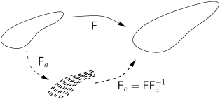
Figure 1. A pictorial representation of the Kröner-Lee decomposition.

The active strain $\mathsf{F}_{a}$ represents a virtual distortion of the relaxed configuration due to activation and only the tensor $\mathsf{F}_{e}$ is responsible for the storing of elastic energy. Then the strain energy density of the active material is given by

(2) $$W_{\text{strain}}(\mathsf{F};\mathsf{F}_{a})=(\det\mathsf{F}_{a})W_{\text{pas}}(\mathsf{F}\mathsf{F}_{a}^{-1}),$$

see for instance [14, 24, 17], and the stress tensor writes

(3) $$\mathsf{P}_{\text{strain}}(\mathsf{F};\mathsf{F}_{a})=(\det\mathsf{F}_{a})\mathsf{P}_{\text{pas}}(\mathsf{F}\mathsf{F}_{a}^{-1})\mathsf{F}_{a}^{-\mathsf{T}},$$

where $\mathsf{P}_{\text{pas}}$ is given by (1).

In the active strain approach the energy density $W_{\text{strain}}$ inherits the same mathematical properties of $W_{\text{pas}}$; for instance, the polyconvexity of the latter ensures the same regularity of the former [18].

In the following sections, we consider an isochoric active strain tensor of the form

(4) $$\mathsf{F}_{a}=(1-a)\boldsymbol{m}\otimes\boldsymbol{m}+\frac{1}{\sqrt{1-a}}(\mathsf{I}-\boldsymbol{m}\otimes\boldsymbol{m}),\qquad 0\leq a<1.$$

Such a choice, which is customary in the literature (see for instance [24, 22, 7]), allows us to obtain the whole tensor $\mathsf{F}_{a}$ by means of a single scalar parameter $a$, accounting for the contraction of the material along the symmetry direction $\boldsymbol{m}$. In the literature, also the case of a non-isochoric $\mathsf{F}_{a}$ has been considered [1, 17, 6], however such a constitutive choice is less popular and will not be taken into consideration in this paper.

Active stress: we additively decompose the total stress as

(5) $$\mathsf{P}_{\text{stress}}(\mathsf{F})=\mathsf{P}_{\text{pas}}(\mathsf{F})+\mathsf{P}_{\text{act}}(\mathsf{F})$$

where $\mathsf{P}_{\text{act}}$, to be constitutively provided, is the stress due to the activation (see for instance [19, 21, 9]).

The formulation given in (5) is quite general. In principle, if we set

$$\mathsf{P}_{\text{act}}(\mathsf{F})=(\det\mathsf{F}_{a})\mathsf{P}_{\text{pas}}(\mathsf{F}\mathsf{F}_{a}^{-1})\mathsf{F}_{a}^{-\mathsf{T}}-\mathsf{P}_{\text{pas}}(\mathsf{F}),$$

then by a suitable choice of the active stress one can recover the active strain approach. However, in the literature the active stress $\mathsf{P}_{\text{act}}$ has to fulfill some modeling prescriptions, which are often incompatible with such a choice.

In the case of transversely isotropic materials with direction of anisotropy $\boldsymbol{m}$, it is usually assumed that $\mathsf{P}_{\text{act}}$ depends on $\mathsf{F}$ only through the pseudo-invariant

$$I_{4}=\mathsf{F}\boldsymbol{m}\cdot\mathsf{F}\boldsymbol{m}$$

in the following way:

(6) $$\mathsf{P}_{\text{act}}(\mathsf{F})=2S(\sqrt{I_{4}})\mathsf{F}\boldsymbol{m}\otimes\boldsymbol{m},$$

where $S$ is a scalar function. One may notice that, according to (6), the non-null components of $\mathsf{P}_{\text{act}}$ are all along $\mathsf{F}\boldsymbol{m}\otimes\boldsymbol{m}$ while in the active strain approach all the components are involved.

Denoting by $W_{\text{act}}$ a primitive function of $S$, one has that

(7) $$\mathsf{P}_{\text{stress}}=\frac{\partial W_{\text{pas}}}{\partial\mathsf{F}}(\mathsf{F})+\frac{W_{\text{act}}^{\prime}(\sqrt{I_{4}})}{\sqrt{I_{4}}}\mathsf{F}\boldsymbol{m}\otimes\boldsymbol{m}-p_{\text{stress}}\mathsf{F}^{-\mathsf{T}}.$$

Remark 1.

It is important to note that $W_{\text{act}}$ should not be physically interpreted as a strain energy density, but only as a primitive function of the active stress. In any case, from a mathematical viewpoint one can define

(8) $$W_{\text{stress}}(\mathsf{F})=W_{\text{pas}}(\mathsf{F})+W_{\text{act}}(\sqrt{I_{4}}).$$

The function $W_{\text{act}}$ can affect the mathematical properties of the total energy, as discussed for instance in [21]. The polyconvexity or the rank-one convexity of the total energy are no more ensured, even if $W_{\text{pas}}$ is convex.

In the next sections we compare the two activation approaches, namely active strain and active stress. We focus on two families of homogeneous deformations: the uniaxial deformation along the direction of anisotropy $\boldsymbol{m}$ and the simple shear orthogonal to $\boldsymbol{m}$. Such a shear modifies the elongation of the body in the direction of anisotropy, so that it allows us to point at differences between the two approaches.

Specifically, we consider the uniaxial incompressible deformation gradient

(9) $$\mathsf{F}_{\lambda}=\lambda\boldsymbol{m}\otimes\boldsymbol{m}+\frac{1}{\sqrt{\lambda}}(\mathsf{I}-\boldsymbol{m}\otimes\boldsymbol{m}),$$

and, given a direction $\boldsymbol{n}$ orthogonal to $\boldsymbol{m}$, the simple shear deformation whose gradient is given by

(10) $$\mathsf{F}_{K}=\mathsf{I}+K\boldsymbol{n}\otimes\boldsymbol{m},$$

where $K$ is the amount of shear (Fig. 2). Notice that in the first case the stretch along the preferred direction $\boldsymbol{m}$ is given by $\lambda$, while in the simple shear it is given by $\sqrt{1+K^{2}}$.

Figure 2. Pictorial representation in the plane of $\boldsymbol{m},\boldsymbol{n}$ of the simple shear (10).

3. Comparing active stress and active strain on a simple shear

In this section we consider an active strain $\mathsf{F}_{a}$ of the form (4) and an active stress $\mathsf{P}_{a}$ of the form (6). Starting from the same passive elastic energy density and imposing that the two activation approaches coincide on uniaxial deformations along the direction of anisotropy, we will compare them on a simple shear.

We consider a homogeneous elastic strain energy density for a transversely isotropic incompressible material of the form

$$W(I_{1},I_{2},I_{4},I_{5}).$$

Then we study the response of the two activation approaches on the uniaxial deformation $\mathsf{F}_{\lambda}$ (9) and on the simple shear $\mathsf{F}_{K}$ (10), while we denote:

$$\mathsf{F}_{\lambda e}=\mathsf{F}_{\lambda}\mathsf{F}_{a}^{-1},\qquad\mathsf{F}_{Ke}=\mathsf{F}_{K}\mathsf{F}_{a}^{-1}.$$

Moreover, let us introduce the notation

$$\mathsf{C}_{e}=\mathsf{F}^{\mathsf{T}}_{e}\mathsf{F}_{e},\quad\mathsf{C}_{\lambda}=\mathsf{F}_{\lambda}^{\mathsf{T}}\mathsf{F}_{\lambda},\quad\mathsf{C}_{\lambda e}=\mathsf{F}_{\lambda e}^{\mathsf{T}}\mathsf{F}_{\lambda e},$$

$$\mathsf{C}_{K}=\mathsf{F}^{\mathsf{T}}_{K}\mathsf{F}_{K},\quad\mathsf{C}_{Ke}=\mathsf{F}_{Ke}^{\mathsf{T}}\mathsf{F}_{Ke}.$$

Then, by (2) and recalling that $\det\mathsf{F}_{a}=1$, the energy density of the material activated with the active strain approach is given by

(11) $$W_{\text{strain}}=W\Big{(}I_{1}(\mathsf{C}_{\lambda e}),I_{2}(\mathsf{C}_{\lambda e}),I_{4}(\mathsf{C}_{\lambda e}),I_{5}(\mathsf{C}_{\lambda e})\Big{)}.$$

On the other hand, by (8) the energy density of the material activated with the active stress approach has the form

(12) $$W_{\text{stress}}=W\Big{(}I_{1}(\mathsf{C}_{\lambda}),I_{2}(\mathsf{C}_{\lambda}),I_{4}(\mathsf{C}_{\lambda}),I_{5}(\mathsf{C}_{\lambda})\Big{)}+W_{\text{act}}\left(\sqrt{I_{4}(\mathsf{C}_{\lambda})}\right).$$

Now we want to find $W_{\text{act}}$ such that the two energy densities (11) and (12) coincide on the deformation $\mathsf{F}_{\lambda}$ for any $\lambda$ and any given value of the activation parameter $a$. Hence we have to choose

(13) $$W_{\text{act}}(\lambda;a)=W\Big{(}I_{1}(\mathsf{C}_{\lambda e}),I_{2}(\mathsf{C}_{\lambda e}),I_{4}(\mathsf{C}_{\lambda e}),I_{5}(\mathsf{C}_{\lambda e})\Big{)}\\ -W\Big{(}I_{1}(\mathsf{C}_{\lambda}),I_{2}(\mathsf{C}_{\lambda}),I_{4}(\mathsf{C}_{\lambda}),I_{5}(\mathsf{C}_{\lambda})\Big{)},$$

where we pointed out the dependence of $W_{\text{act}}$ on the amount of stretch and on the activation parameter.

For a general deformation $\mathsf{F}$, the elastic energy density corresponding to the active strain model will be directly computed using $W(I_{1}(\mathsf{C}_{e}),I_{2}(\mathsf{C}_{e}),I_{4}(\mathsf{C}_{e}),I_{5}(\mathsf{C}_{e}))$. On the contrary, the elastic energy density corresponding to the active stress model will be given by

$$W(I_{1},I_{2},I_{4},I_{5})+W_{\text{act}}(\sqrt{I_{4}};a),$$

where the function $W_{\text{act}}$ is given in (13).

We now consider the simple shear deformation $\mathsf{F}_{K}$ given by (10). In this case we have $\sqrt{I_{4}(\mathsf{C}_{K})}=\sqrt{1+K^{2}}$ and

$$I_{1}(\mathsf{C}_{Ke})=\frac{1+K^{2}}{(1-a)^{2}}+2(1-a),\quad I_{2}(\mathsf{C}_{Ke})=\frac{2+K^{2}}{1-a}+(1-a)^{2},$$

$$I_{4}(\mathsf{C}_{Ke})=\frac{1+K^{2}}{(1-a)^{2}},\quad I_{5}(\mathsf{C}_{Ke})=\frac{(1+K^{2})^{2}}{(1-a)^{4}}+\frac{K^{2}}{1-a},$$

$$I_{1}(\mathsf{C}_{K})=3+K^{2},\quad I_{2}(\mathsf{C}_{K})=3+K^{2},$$

$$I_{4}(\mathsf{C}_{K})=1+K^{2},\quad I_{5}(\mathsf{C}_{K})=K^{2}+(1+K^{2})^{2},$$

$$I_{1}(\mathsf{C}_{\lambda e})=\frac{1+K^{2}}{(1-a)^{2}}+2\frac{1-a}{\sqrt{1+K^{2}}},\quad I_{2}(\mathsf{C}_{\lambda e})=\frac{(1-a)^{2}}{1+K^{2}}+2\frac{\sqrt{1+K^{2}}}{1-a},$$

$$I_{4}(\mathsf{C}_{\lambda e})=\frac{1+K^{2}}{(1-a)^{2}},\quad I_{5}(\mathsf{C}_{\lambda e})=\frac{(1+K^{2})^{2}}{(1-a)^{4}},$$

$$I_{1}(\mathsf{C}_{\lambda})=1+K^{2}+\frac{2}{\sqrt{1+K^{2}}},\quad I_{2}(\mathsf{C}_{\lambda})=\frac{1}{1+K^{2}}+2\sqrt{1+K^{2}},$$

$$I_{4}(\mathsf{C}_{\lambda})=1+K^{2},\quad I_{5}(\mathsf{C}_{\lambda})=(1+K^{2})^{2}.$$

Imposing that active strain and active stress have the same energy density (and hence the same stress tensor field) both on every uniaxial deformation $\mathsf{F}_{\lambda}$ and every simple shear $\mathsf{F}_{K}$, then

$$W\Big{(}I_{1}(\mathsf{C}_{Ke}),I_{2}(\mathsf{C}_{Ke}),I_{4}(\mathsf{C}_{Ke}),I_{5}(\mathsf{C}_{Ke})\Big{)}\\ =W(I_{1}(\mathsf{C}_{K}),I_{2}(\mathsf{C}_{K}),I_{4}(\mathsf{C}_{K}),I_{5}(\mathsf{C}_{K}))+W_{\text{act}}(\sqrt{1+K^{2}};a),$$

where the function $W_{\text{act}}$ is given in (13).

Hence for every $0\leq a<1$ and $K\geq 0$ one has

$$W\left(\frac{1+K^{2}}{(1-a)^{2}}+2(1-a),\frac{2+K^{2}}{1-a}+(1-a)^{2},\frac{1+K^{2}}{(1-a)^{2}},\frac{(1+K^{2})^{2}}{(1-a)^{4}}+\frac{K^{2}}{1-a}\right)$$

$$- W\left(\frac{1+K^{2}}{(1-a)^{2}}+2\frac{1-a}{\sqrt{1+K^{2}}},\frac{(1-a)^{2}}{1+K^{2}}+2\frac{\sqrt{1+K^{2}}}{1-a},\frac{1+K^{2}}{(1-a)^{2}},\frac{(1+K^{2})^{2}}{(1-a)^{4}}\right)$$

$$= W\left(3+K^{2},3+K^{2},1+K^{2},K^{2}+(1+K^{2})^{2}\right)$$

$$- W\left(1+K^{2}+\frac{2}{\sqrt{1+K^{2}}},\frac{1}{1+K^{2}}+2\sqrt{1+K^{2}},1+K^{2},(1+K^{2})^{2}\right).$$

Setting for convenience $1+K^{2}=\ell^{2}$ and $\frac{1}{1-a}=x$, the equation becomes

(14) $$W\left({\ell^{2}}{x^{2}}+\frac{2}{x},(1+\ell^{2})x+\frac{1}{x^{2}},{\ell^{2}}{x^{2}},{\ell^{4}}{x^{4}}+(\ell^{2}-1){x}\right)$$

$$- W\left({\ell^{2}}{x^{2}}+\frac{2}{\ell x},\frac{1}{\ell^{2}x^{2}}+{2\ell}{x},{\ell^{2}}{x^{2}},{\ell^{4}}{x^{4}}\right)$$

$$= W\left(2+\ell^{2},2+\ell^{2},\ell^{2},\ell^{4}+\ell^{2}-1\right)-W\left(\ell^{2}+\frac{2}{\ell},\frac{1}{\ell^{2}}+2\ell,\ell^{2},\ell^{4}\right).$$

Differentiating w.r.t. $\ell$ and letting $\ell\to 1$ one gets

$$\frac{\partial W}{\partial I_{1}}\left(x^{2}+\frac{2}{x},\frac{1}{x^{2}}+2x,x^{2},x^{4}\right)$$

$$+\frac{1}{x} \frac{\partial W}{\partial I_{2}}\left(x^{2}+\frac{2}{x},\frac{1}{x^{2}}+2x,x^{2},x^{4}\right)$$

$$+x^{2} \frac{\partial W}{\partial I_{5}}\left(x^{2}+\frac{2}{x},\frac{1}{x^{2}}+2x,x^{2},x^{4}\right)$$

$$=x \left(\frac{\partial W}{\partial I_{1}}(3,3,1,1)+\frac{\partial W}{\partial I_{2}}(3,3,1,1)+\frac{\partial W}{\partial I_{5}}(3,3,1,1)\right).$$

On the other hand, differentiating w.r.t. $x$ and letting $x\to 1$ one gets

$$2(\ell^{2}-1)\ell^{2} \frac{\partial W}{\partial I_{1}}\left(2+\ell^{2},2+\ell^{2},\ell^{2},\ell^{4}+\ell^{2}-1\right)$$

$$+(\ell^{2}-1)\ell^{2} \frac{\partial W}{\partial I_{2}}\left(2+\ell^{2},2+\ell^{2},\ell^{2},\ell^{4}+\ell^{2}-1\right)$$

$$+2\ell^{4} \frac{\partial W}{\partial I_{4}}\left(2+\ell^{2},2+\ell^{2},\ell^{2},\ell^{4}+\ell^{2}-1\right)$$

$$+\ell^{2}(4\ell^{4}+\ell^{2}-1) \frac{\partial W}{\partial I_{5}}\left(2+\ell^{2},2+\ell^{2},\ell^{2},\ell^{4}+\ell^{2}-1\right)$$

$$=2\ell(\ell^{3}-1) \frac{\partial W}{\partial I_{1}}\left(\ell^{2}+\frac{2}{{\ell}},\frac{1}{\ell^{2}}+2{\ell},\ell^{2},\ell^{4}\right)$$

$$+2(\ell^{3}-1) \frac{\partial W}{\partial I_{2}}\left(\ell^{2}+\frac{2}{{\ell}},\frac{1}{\ell^{2}}+2{\ell},\ell^{2},\ell^{4}\right)$$

$$+2\ell^{4} \frac{\partial W}{\partial I_{4}}\left(\ell^{2}+\frac{2}{{\ell}},\frac{1}{\ell^{2}}+2{\ell},\ell^{2},\ell^{4}\right)$$

$$+4\ell^{6} \frac{\partial W}{\partial I_{5}}\left(\ell^{2}+\frac{2}{{\ell}},\frac{1}{\ell^{2}}+2{\ell},\ell^{2},\ell^{4}\right).$$

By taking the mixed second derivative of (14) and letting both $x\to 1$ and $\ell\to 1$, one gets

$$\frac{\partial W}{\partial I_{1}}\left(3,3,1,1\right)+2\frac{\partial W}{\partial I_{2}}\left(3,3,1,1\right)-\frac{\partial W}{\partial I_{5}}\left(3,3,1,1\right)\\ =2\frac{\partial^{2}W}{\partial I_{1}I_{4}}\left(3,3,1,1\right)+4\frac{\partial^{2}W}{\partial I_{1}I_{5}}\left(3,3,1,1\right)+2\frac{\partial^{2}W}{\partial I_{2}I_{4}}\left(3,3,1,1\right)\\ +4\frac{\partial^{2}W}{\partial I_{2}I_{5}}\left(3,3,1,1\right)+2\frac{\partial^{2}W}{\partial I_{4}I_{5}}\left(3,3,1,1\right)+4\frac{\partial^{2}W}{\partial I_{5}^{2}}\left(3,3,1,1\right)$$

which gives a very particular relation for the elastic moduli in the identity. For instance, imposing the previous condition on the energy density (27) considered in Sect. 5, which depends also on $I_{5}$, we get the necessary condition

$$2(\alpha+2\beta)w_{0}^{2}-(2\alpha+10\beta+3)w_{0}+6(\beta+1)=0$$

which holds only for very special values of the constitutive parameters.

Even if we drop out the dependence of the energy on $I_{5}$, as we will do in the sequel, from (14) we have

(15) $$W\left(\ell^{2}x^{2}+\frac{2}{x},(1+\ell^{2})x+\frac{1}{x^{2}},\ell^{2}x^{2}\right)-W\left(\ell^{2}x^{2}+\frac{2}{\ell x},\frac{1}{\ell^{2}x^{2}}+2\ell x,\ell^{2}x^{2}\right)\\ =W\left(2+\ell^{2},2+\ell^{2},\ell^{2}\right)-W\left(\ell^{2}+\frac{2}{\ell},\frac{1}{\ell^{2}}+2\ell,\ell^{2}\right),$$

for every $x\geq 1$ and $\ell\geq 1$.

Condition (15) results to be very restrictive and rules out any typical energy density used for elastic materials. Indeed, the only elastic energy density that we have found to satisfy the equivalence between active stress and active strain both on $\mathsf{F}_{\lambda}$ and on $\mathsf{F}_{K}$ is

$$W(I_{1},I_{4})=cI_{1}\sqrt{I_{4}}+f(I_{4}).$$

In such a case, eq. (15) is satisfied for any $x,\ell\geq 1$. However, that energy has a very particular form and we are not aware of any model of nonlinear elasticity where it is used.

3.1. The fiber-reinforced case

Among the transversely isotropic media, an important role is played by the so-called fiber-reinforced materials, for which the strain energy density splits as a sum of isotropic and anisotropic contributions. For the sake of simplicity, we will assume that the anisotropic term does not depend on $I_{5}$, so that

$$W=W_{\text{iso}}(I_{1},I_{2})+W_{\text{aniso}}(I_{4}).$$

Then (15) becomes

(16) $$W_{\text{iso}}\left(\ell^{2}x^{2}+\frac{2}{x},(1+\ell^{2})x+\frac{1}{x^{2}}\right)-W_{\text{iso}}\left(\ell^{2}x^{2}+\frac{2}{\ell x},\frac{1}{\ell^{2}x^{2}}+2\ell x\right)\\ =W_{\text{iso}}\left(2+\ell^{2},2+\ell^{2}\right)-W_{\text{iso}}\left(\ell^{2}+\frac{2}{\ell},\frac{1}{\ell^{2}}+2\ell\right),$$

for every $x\geq 1$ and $\ell\geq 1$.

Differentiating w.r.t. $\ell$ and letting $\ell=1$ one gets

(17) $$\frac{\partial W_{\text{iso}}}{\partial I_{1}}\left(x^{2}+\frac{2}{x},\frac{1}{x^{2}}+2x\right)+\frac{1}{x}\frac{\partial W_{\text{iso}}}{\partial I_{2}}\left(x^{2}+\frac{2}{x},\frac{1}{x^{2}}+2x\right)\\ =x\left(\frac{\partial W_{\text{iso}}}{\partial I_{1}}(3,3)+\frac{\partial W_{\text{iso}}}{\partial I_{2}}(3,3)\right).$$

On the other hand, differentiating w.r.t. $x$ and letting $x=1$ one gets

(18) $$2(\ell^{2}-1)\ell^{2}\frac{\partial W_{\text{iso}}}{\partial I_{1}}\left(2+\ell^{2},2+\ell^{2}\right)+(\ell^{2}-1)\ell^{2}\frac{\partial W_{\text{iso}}}{\partial I_{2}}\left(2+\ell^{2},2+\ell^{2}\right)\\ =2\ell(\ell^{3}-1)\frac{\partial W_{\text{iso}}}{\partial I_{1}}\left(\ell^{2}+\frac{2}{{\ell}},\frac{1}{\ell^{2}}+2{\ell}\right)+2(\ell^{3}-1)\frac{\partial W_{\text{iso}}}{\partial I_{2}}\left(\ell^{2}+\frac{2}{{\ell}},\frac{1}{\ell^{2}}+2{\ell}\right).$$

By taking the mixed (second) derivative of (15) and letting both $x=1$ and $\ell=1$, one gets

(19) $$\frac{\partial W_{\text{iso}}}{\partial I_{1}}\left(3,3\right)+2\frac{\partial W_{\text{iso}}}{\partial I_{2}}\left(3,3\right)=0.$$

Eqs. (17)–(19) represent some necessary conditions for the passive energy density $W$ in order to produce the same results with the two activation approaches on uniaxial deformations and on simple shears. Eq. (17) is notably severe: a particular combination of the two partial derivatives of the energy has to be constant for any $x$. For instance, in the case of fiber-reinforced Mooney-Rivlin materials, where

$$W(I_{1},I_{2},I_{4})=c_{1}(I_{1}-3)+c_{2}(I_{2}-3)+f(I_{4}),$$

it follows immediately from (17) that

$$c_{1}+\frac{c_{2}}{x}=x(c_{1}+c_{2})\quad\Rightarrow\quad\frac{c_{2}}{c_{1}+c_{2}}=-x\quad\text{for any $x\geq 1$},$$

which is impossible. Hence, in the case of a fiber-reinforced Mooney-Rivlin material active stress and active strain are never equivalent.

Also the important case where $W_{\text{iso}}$ depends only on $I_{1}$ is always ruled out, since condition (19) becomes $W^{\prime}_{\text{iso}}(3)=0$ and by (17) we get

$$W^{\prime}_{\text{iso}}(I_{1})=0\quad\text{for any $I_{1}\geq 3$},$$

whence $W_{\text{iso}}$ is a constant.

Coming back to the general fiber-reinforced case, we can also take the third derivative of (16), twice w.r.t. $\ell$ and once w.r.t. $x$. Letting $x=\ell=1$ we get the relation

(20) $$2\frac{\partial W_{\text{iso}}}{\partial I_{1}}(3,3)+7\frac{\partial W_{\text{iso}}}{\partial I_{2}}(3,3)+8\frac{\partial^{2}W_{\text{iso}}}{\partial I_{1}^{2}}(3,3)\\ +12\frac{\partial^{2}W_{\text{iso}}}{\partial I_{1}\partial I_{2}}(3,3)+4\frac{\partial^{2}W_{\text{iso}}}{\partial I_{2}^{2}}(3,3)=0.$$

On the other hand, taking the third derivative twice w.r.t. $x$ and once w.r.t. $\ell$ and letting $x=\ell=1$ we get

(21) $$\frac{\partial W_{\text{iso}}}{\partial I_{1}}(3,3)+3\frac{\partial W_{\text{iso}}}{\partial I_{2}}(3,3)+3\frac{\partial^{2}W_{\text{iso}}}{\partial I_{1}^{2}}(3,3)\\ +6\frac{\partial^{2}W_{\text{iso}}}{\partial I_{1}\partial I_{2}}(3,3)+3\frac{\partial^{2}W_{\text{iso}}}{\partial I_{2}^{2}}(3,3)=0.$$

By combining (19), (20) and (21) we get the following necessary condition involving the second derivatives of the isotropic part of the energy density in the identity deformation:

(22) $$\frac{\partial^{2}W_{\text{iso}}}{\partial I_{1}^{2}}(3,3)+6\frac{\partial^{2}W_{\text{iso}}}{\partial I_{1}\partial I_{2}}(3,3)+5\frac{\partial^{2}W_{\text{iso}}}{\partial I_{2}^{2}}(3,3)=0.$$

For instance, isotropic energy densities of the kind

$$W_{\text{iso}}(I_{1},I_{2})=c_{1}(I_{1}-3)^{2}+c_{12}(I_{1}-3)(I_{2}-3)+c_{2}(I_{2}-3)^{2}$$

satisfy the last condition only for a very particular choice of the elastic moduli.

4. A quantitative example

In this section we highlight that the differences between the two activation approaches can be considerable, even if the passive energy is quite simple, as in the case of a Mooney-Rivlin material with a transversely isotropic reinforcing term:

(23) $$W_{\text{pas}}(\mathsf{F})=c_{1}(I_{1}-3)+c_{2}(I_{2}-3)+c_{3}(\sqrt{I_{4}}-1)^{2}.$$

Sect. 5 will be devoted to a more refined energy which is commonly used for modeling skeletal muscle tissue.

Let us assume an active strain of the form (4) and deduce the corresponding active part of the energy $W_{\text{act}}$ which gives the same stress on the uniaxial deformation $\mathsf{F}_{\lambda}$ (9). The energy density of the active strain approach is

$$W_{\text{strain}}(\lambda;a)=W_{\text{pas}}(\mathsf{F}_{\lambda}\mathsf{F}_{a}^{-1})\\ =c_{1}\left(\frac{\lambda^{2}}{(1-a)^{2}}+\frac{2(1-a)}{\lambda}-3\right)\\ +c_{2}\left(\frac{(1-a)^{2}}{\lambda^{2}}+\frac{2\lambda}{1-a}-3\right)+c_{3}\left(\frac{\lambda}{1-a}-1\right)^{2},$$

and the passive part is given by $W_{\text{pas}}(\lambda)=W_{\text{strain}}(\lambda;0)$. As in the previous section, recalling that $W_{\text{stress}}=W_{\text{pas}}+W_{\text{act}}$, the function $W_{\text{act}}$ such that the two energies coincide on the deformation $\mathsf{F}_{\lambda}$ is

(24) $$W_{\text{act}}(\lambda;a)=W_{\text{strain}}(\lambda;a)-W_{\text{strain}}(\lambda;0)\\ =a\left[c_{1}\left(\frac{2-a}{(1-a)^{2}}\lambda^{2}-\frac{2}{\lambda}\right)+c_{2}\left(\frac{2}{1-a}\lambda-\frac{2-a}{\lambda^{2}}\right)+c_{3}\frac{\lambda}{1-a}\left(\frac{2-a}{1-a}\lambda-2\right)\right].$$

Fig. 3 shows the profile of the stress and of its active part along the uniaxial deformations for several values of the activation parameter $a$. From now on we fix $c_{1}=4$kPa, $c_{2}=20$kPa, $c_{3}=40$kPa. Denoting by $P^{mm}$ and $P_{\text{act}}^{mm}$ the components along $\boldsymbol{m}\otimes\boldsymbol{m}$ of the total and active stress, respectively, one can see that $P^{mm}$ and $P_{\text{act}}^{mm}$ increase, as the parameter $a$ increases.

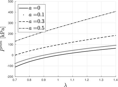
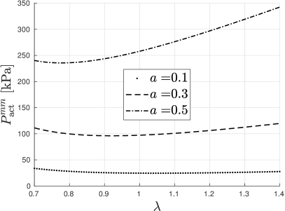
Figure 3. On the left: stress-stretch relation obtained on the uniaxial deformation along the direction of anisotropy. On the right: active part of the stress.

On a general deformation $\mathsf{F}$, the stresses corresponding to the active strain and the active stress models will be directly computed using (3) and (7), respectively. Taking into account incompressibility, we have

$$\mathsf{P}_{\text{strain}}= \left(2c_{1}\mathsf{F}_{e}+2c_{2}(I_{1}(\mathsf{C}_{e})\mathsf{F}_{e}-\mathsf{F}_{e}\mathsf{F}_{e}^{\mathsf{T}}\mathsf{F}_{e})+2c_{3}(\sqrt{I_{4}(\mathsf{C}_{e})}-1)\frac{1}{\sqrt{I_{4}(\mathsf{C}_{e})}}\mathsf{F}_{e}\boldsymbol{m}\otimes\boldsymbol{m}\right)\mathsf{F}_{a}^{-\mathsf{T}}$$

$$-p_{\text{strain}}\mathsf{F}^{-\mathsf{T}},$$

$$\mathsf{P}_{\text{stress}}= 2c_{1}\mathsf{F}+2c_{2}(I_{1}\mathsf{F}-\mathsf{F}\mathsf{F}^{\mathsf{T}}\mathsf{F})+2c_{3}(\sqrt{I_{4}}-1)\frac{1}{\sqrt{I_{4}}}\mathsf{F}\boldsymbol{m}\otimes\boldsymbol{m}+\frac{W_{\text{act}}^{\prime}(\sqrt{I_{4}})}{\sqrt{I_{4}}}\mathsf{F}\boldsymbol{m}\otimes\boldsymbol{m}$$

$$-p_{\text{stress}}\mathsf{F}^{-\mathsf{T}}.$$

Let us analyze the response of the two approaches on the simple shear $\mathsf{F}_{K}$ given by (10). We will follow the classical assumption of plane stress in order to find the unknown pressure fields $p_{\text{strain}}$ and $p_{\text{stress}}$, that is $P_{\text{strain}}^{ss}=0$ and $P_{\text{stress}}^{ss}=0$, where $\boldsymbol{s}=\boldsymbol{m}\times\boldsymbol{n}$. Another possibility, which will not be taken into consideration in this paper, is to assume zero normal traction on the inclined faces; for a discussion, see [13].

The non-vanishing components of the stresses are given by

(25) $$P_{\text{strain}}^{mm}= 2c_{1}\left(\frac{1}{(1-a)^{2}}-(1-a)\right)+2c_{2}\left(\frac{1-K^{2}}{1-a}-(1-a)^{2}\right)+\frac{2c_{3}}{1-a}\left(\frac{1}{1-a}-\frac{1}{\sqrt{1+K^{2}}}\right),$$

$$P_{\text{stress}}^{mm}= 2c_{1}a\left(\frac{2-a}{(1-a)^{2}}+\frac{1}{(1+K^{2})^{3/2}}\right)+2c_{2}\left(\frac{a(2-a)}{(1+K^{2})^{2}}+\frac{a}{(1-a)\sqrt{1+K^{2}}}-K^{2}\right)$$

$$+\frac{2c_{3}}{1-a}\left(\frac{1}{1-a}-\frac{1}{\sqrt{1+K^{2}}}\right),$$

$$P_{\text{strain}}^{mn}= 2c_{1}K(1-a)+2c_{2}K\left(\frac{K^{2}}{1-a}+(1-a)^{2}\right),$$

$$P_{\text{stress}}^{mn}= 2K\Big{(}c_{1}+c_{2}(1+K^{2})\Big{)}=P_{\text{pas}}^{mn},$$

$$P_{\text{strain}}^{nm}= 2c_{1}\frac{K}{(1-a)^{2}}+2c_{2}\frac{K}{1-a}+2c_{3}\frac{K}{(1-a)}\left(\frac{1}{1-a}-\frac{1}{\sqrt{1+K^{2}}}\right),$$

$$P_{\text{stress}}^{nm}= 2c_{1}K\left(\frac{1}{(1-a)^{2}}+\frac{a}{(1+K^{2})^{3/2}}\right)+2c_{2}K\left(1+\frac{a(2-a)}{(1+K^{2})^{2}}+\frac{a}{(1-a)\sqrt{1+K^{2}}}\right)$$

$$+2c_{3}\frac{K}{1-a}\left(\frac{1}{1-a}-\frac{1}{\sqrt{1+K^{2}}}\right),$$

$$P_{\text{strain}}^{nn}= -2c_{2}\frac{K^{2}}{1-a},$$

$$P_{\text{stress}}^{nn}= -2c_{2}K^{2}=P_{\text{pas}}^{nn}.$$

In Fig. 4 we plot such components with respect to the amount of shear $K$, both in the case of active strain and of active stress. As one can see, even if the two activation approaches produce the same stress tensor on uniaxial deformations along the direction of anisotropy, the stresses are different on the simple shear $\mathsf{F}_{K}$.

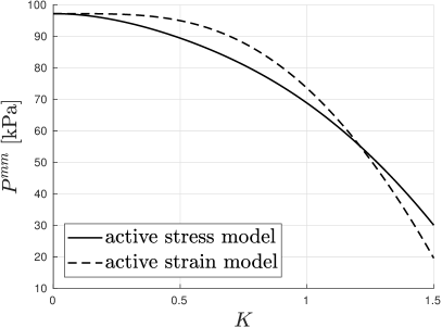
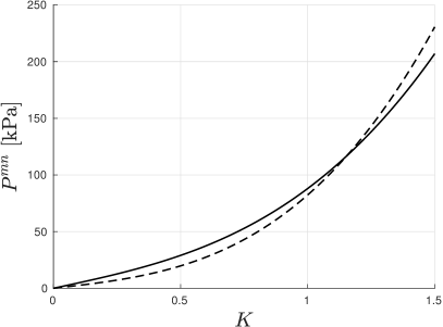
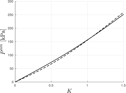
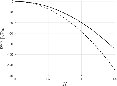
Figure 4. Comparison between the stress components of the two activation approaches when $a=0.3$.

The dependence of the differences between $\mathsf{P}_{\text{stress}}$ and $\mathsf{P}_{\text{strain}}$ on the activation parameter $a$ is showed in Fig. 5: such a difference is more evident when $a$ increases. As we have already noticed, the active part of $\mathsf{P}_{\text{stress}}$ lies along $\mathsf{F}_{K}\boldsymbol{m}\otimes\boldsymbol{m}$, so that $P^{mn}_{\text{stress}}$ and $P^{nn}_{\text{stress}}$ in (25) do not depend on $a$. Hence the plots on the right in Fig. 5 represent the differences between $\mathsf{P}_{\text{pas}}$ and $\mathsf{P}_{\text{strain}}$ along $\boldsymbol{m}\otimes\boldsymbol{n}$ and $\boldsymbol{n}\otimes\boldsymbol{n}$.

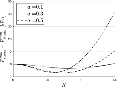
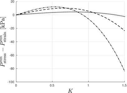
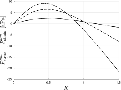
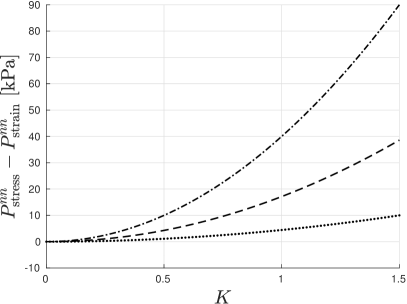
Figure 5. Differences between the components of the stress in the two activation approaches for several value of the activation parameter $a$.

5. A more complex energy related to skeletal muscle tissue

As an important example, we now consider the case of the activation of a skeletal muscle tissue, for which there are several experimental data on uniaxial deformations. In this case it is easier to measure the active stress $\mathsf{P}_{\text{act}}$ than the active strain $\mathsf{F}_{a}$: indeed, the components of the active stress can be obtained by computing the difference between the data collected in the active and passive case, see for instance [26, 8]. Hence, differently from the previous sections, we start from a given active stress and find a suitable active strain that produces the same results in the uniaxial deformations along the direction of anisotropy.

As far as the passive energy and the active stress are concerned, we will follow the model given in [4], while the active strain will be modeled as in [7]. We will compare the stress components along a cross-fiber simple shear obtained by exploiting the two activation approaches.

The typical active stress-stretch curve reaches a maximum point at $\lambda_{\text{opt}}$ and then decreases for larger values of $\lambda$, see for instance [8] for the tetanized tibialis anterior of a rat. Following [4], we assume that the active part of the stress is

(26) $$P_{\text{act}}^{mm}(\lambda)=\left\{\begin{aligned} &P_{\text{opt}}\frac{\lambda_{\text{min}}-\lambda}{\lambda_{\text{min}}-\lambda_{\text{opt}}}e^{\frac{(2\lambda_{\text{min}}-\lambda-\lambda_{\text{opt}})(\lambda-\lambda_{\text{opt}})}{2(\lambda_{\text{min}}-\lambda_{\text{opt}})^{2}}}&\text{if $\lambda>\lambda_{\text{min}}$},\\[4.30554pt] &0&\text{otherwise},\end{aligned}\right.$$

where $\lambda_{\text{min}}$ is the minimum stretch value after which the activation starts, while $(\lambda_{\text{opt}},P_{\text{opt}})$ identifies the maximum of the curve. According to [4], we set $\lambda_{\text{min}}=0.682$, $\lambda_{\text{opt}}=1.192$, $P_{\text{opt}}=73.52$kPa. Fig. 6 shows that the curve fits quite well the active data obtained in [8].

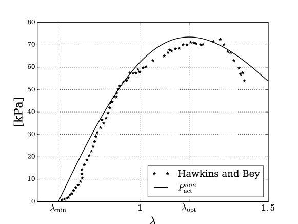
Figure 6. Plot of (26) together with the representation of the experimental data given in [8].

Since (26) represents the component of $\mathsf{P}_{\text{act}}$ along $\mathsf{F}\boldsymbol{m}\otimes\boldsymbol{m}$, for the active stress case it is enough to compute a primitive function in order to write the energy density $W_{\text{act}}$. Denoting by $\sqrt{I_{4}}$ the stretch along the direction of anisotropy $\boldsymbol{m}$ in a general deformation, we have

$$W_{\text{act}}(\sqrt{I_{4}})=\left\{\begin{aligned} &P_{\text{opt}}(\lambda_{\text{min}}-\lambda_{\text{opt}})\left(e^{\frac{(2\lambda_{\text{min}}-\sqrt{I_{4}}-\lambda_{\text{opt}})(\sqrt{I_{4}}-\lambda_{\text{opt}})}{2(\lambda_{\text{min}}-\lambda_{\text{opt}})^{2}}}-e^{1/2}\right)&\text{if $\lambda>\lambda_{\text{min}}$},\\ &0&\text{otherwise}.\end{aligned}\right.$$

Notice that the experimental data show that the active part of the stress is not monotone, hence the corresponding total strain energy can lose the rank-one convexity.

As far as the passive part is concerned, following again the model given in [4] and [7], we use the exponential strain energy density function

(27) $$W_{\text{pas}}^{\text{muscle}}=\frac{\mu}{4}\left\{\frac{1}{\alpha}\left[e^{\alpha({I}_{p}-1)}-1\right]+\frac{1}{\beta}\left[e^{\beta(K_{p}-1)}-1\right]\right\},$$

where

$${I}_{p} =\frac{w_{0}}{3}\operatorname{tr}({\mathsf{C}})+(1-w_{0})\operatorname{tr}({\mathsf{C}}{\boldsymbol{m}\otimes\boldsymbol{m}}),$$

$$K_{p} =\frac{w_{0}}{3}\operatorname{tr}({{\mathsf{C}}^{-1}})+(1-w_{0})\operatorname{tr}({\mathsf{C}}^{-1}{\boldsymbol{m}\otimes\boldsymbol{m}})$$

(here $\boldsymbol{m}$ is the direction of the muscular fibers). Notice that in the incompressible case $I_{p}$ and $K_{p}$ can be expressed in terms of the usual invariants as

$${I}_{p}=\frac{w_{0}}{3}I_{1}+(1-w_{0})I_{4},\ \ K_{p}=\frac{w_{0}}{3}I_{2}+(1-w_{0})(I_{5}-I_{1}I_{4}+I_{2}).$$

The material parameters $\alpha=19.69$, $\beta=1.190$, $w_{0}=0.7388$ and $\mu=0.1599$kPa given in [4] are obtained from the passive data about the tibialis anterior of a rat [8]; in particular, $w_{0}$ measures the amount of anisotropy of the material.

Now that the active stress and the passive energy have been chosen, we want to find a suitable active strain which gives the same results on uniaxial deformations. The issue is subtle because we cannot assume that $\mathsf{F}_{a}$ is constant. Indeed one can see that a constant active strain cannot fit at all the experimental data. To address this problem we will assume that $\mathsf{F}_{a}$ depends on the deformation gradient $\mathsf{F}$, see also [4, 6, 7, 5, 25]. Such an approach, which is a generalization of the active strain, is crucial in the applications to skeletal muscle: it allows to capture the physics of a muscle, in which the stress produced when the tissue is activated depends on strain. In this case the mathematical properties of $W_{\text{strain}}$ can change considerably and $\mathsf{F}_{a}$ does not represent anymore the local distortion of the material that maps the reference configuration to the relaxed one. Moreover, the expression of the stress tensor is much more involved, see [7]:

(28) $$P_{\text{strain}}^{hk}(\mathsf{F})=\frac{\partial W_{\text{strain}}}{\partial F^{hk}}(\mathsf{F};\mathsf{F}_{a}(\mathsf{F}))+\frac{\partial W_{\text{strain}}}{\partial F_{a}^{ij}}(\mathsf{F};\mathsf{F}_{a}(\mathsf{F}))\frac{\partial F_{a}^{ij}}{\partial F^{hk}}(\mathsf{F})-p_{\text{strain}}(\mathsf{F}^{-\mathsf{T}})^{hk},$$

with $h,k=1,2,3$.

Given an active strain $\mathsf{F}_{a}$ as in (4), we assume that the activation parameter $a$ depends on the stretch of the fibers. Along the uniaxial deformation $\mathsf{F}_{\lambda}$ (9) we have that $a$ is a function of $\lambda$. Imposing that the energies of the active stress and of the active strain formulation coincide on $\mathsf{F}_{\lambda}$, we look for $a(\lambda)$ such that

(29) $$W_{\text{strain}}(\lambda;a(\lambda))=W_{\text{pas}}^{\text{muscle}}(\lambda)+W_{\text{act}}(\lambda).$$

Since the parameter $a$ accounts for a contraction, we recall that $0\leq a(\lambda)<1$. Eq. (29) admits the solution $a(\lambda)=0$ whenever $W_{\text{act}}(\lambda)=0$, but in general it is too complicated to solve analytically. In Fig. 7 we plot a numerical approximation of the solution $a(\lambda)$: the function is discontinuous at $\lambda_{\text{min}}$ and vanishes as $\lambda\to+\infty$.

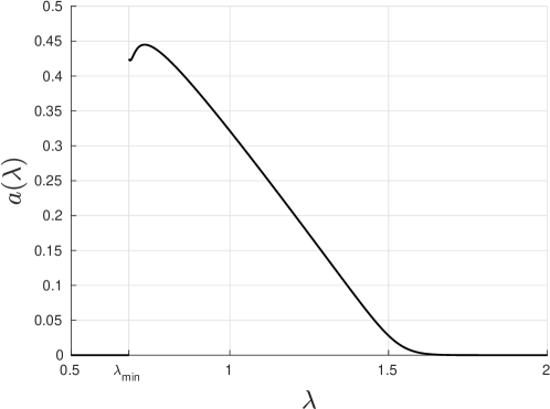
Figure 7. Plot of the function $a(\lambda)$ solution of (29).

Now that the two approaches give the same stress along the uniaxial deformations $\mathsf{F}_{\lambda}$, let us consider the simple shear $\mathsf{F}_{K}$ (10). Assuming as in the previous section that $P_{\text{strain}}^{ss}=0$ and $P_{\text{stress}}^{ss}=0$, where $\boldsymbol{s}=\boldsymbol{m}\times\boldsymbol{n}$, we can find the Lagrange multipliers related to the incompressibility constraint. Also in this case we have that active stress and active strain do not produce the same stress on a simple shear. The non-vanishing components of the stresses along the simple shear (10) are showed in Fig. 8. We notice that the exponential form of the energy amplifies the differences between the two activation approaches, as already remarked in [23].

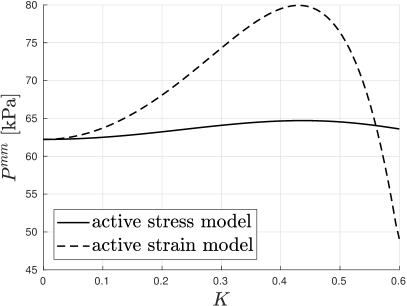
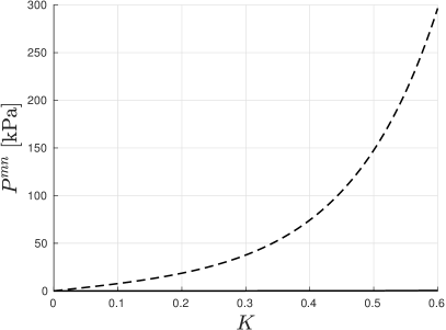
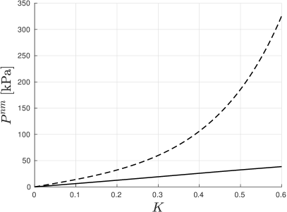
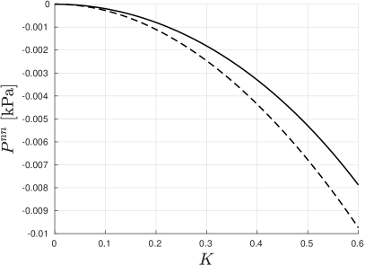
Figure 8. Comparison between the stress components of the two activation approaches in the case of energy (27), Sect. 5. Here we considered only values of $K$ up to $0.6$, which is the physiological range for a skeletal muscle tissue.

6. Decoupled active strain approach

Active stress and active strain are by far the two most used methods in the continuum modeling of activation, at least for biological tissues; however, other approaches can be found in the literature. In this brief section we study one of them, which is a sort of active strain applied only to a part of the energy [12, 20]. We will see that such an approach is equivalent to an active strain.

Let us consider a passive energy of the form

$$W_{\text{pas}}=W(\mathsf{F})+W_{\text{aniso}}(I_{4})$$

(for instance, if $W$ is assumed to be isotropic, we get the fiber-reinforced materials introduced in Sect. 3.1). Now apply the Kröner-Lee decomposition only to $W_{\text{aniso}}$, so that the energy of the active material is given by

$$W_{\text{decoup}}=W(\mathsf{F})+(\det\mathsf{F}_{a})W_{\text{aniso}}(I_{4}(\mathsf{C}_{e})).$$

We name decoupled active strain such an approach. Notice that in the full active strain method one should compute also $W$ on the elastic part $\mathsf{F}_{e}=\mathsf{F}\mathsf{F}_{a}^{-1}$, as in (2).

Let us assume that $\mathsf{F}_{a}$ can depend on the deformation gradient $\mathsf{F}$ only through the invariant $I_{4}$ and that $\boldsymbol{m}$ is an eigenvector of $\mathsf{F}_{a}$ (for instance, if $a$ is a function only of $I_{4}$, the active strain (4) satisfies the two assumptions). Then we claim that

the decoupled active strain is completely equivalent to an active stress approach.

Indeed, we prove that there exists a suitable energy density $W_{\text{act}}(\sqrt{I_{4}})$ such that

$$W_{\text{stress}}=W_{\text{pas}}+W_{\text{act}}=W_{\text{decoup}}$$

on every deformation. Hence, the two methods produce the same stress even in the case of simple shear.

Indeed, the two energies coincide if

(30) $$W_{\text{act}}(\sqrt{I_{4}})=W_{\text{aniso}}(I_{4}(\mathsf{C}_{e}))-W_{\text{aniso}}(I_{4}),$$

but in general the quantity $I_{4}(\mathsf{C}_{e})$ depends on the whole $\mathsf{F}$ and not only on $I_{4}$. However, in the case when $\boldsymbol{m}$ is an eigenvector of $\mathsf{F}_{a}$, it is easy to verify that

$$I_{4}(\mathsf{C}_{e})=\frac{I_{4}}{I_{4}(\mathsf{C}_{a})},$$

where $\mathsf{C}_{a}=\mathsf{F}_{a}^{\mathsf{T}}\mathsf{F}_{a}$. Moreover, we assumed that $\mathsf{F}_{a}$ is a function only of $I_{4}$, hence (30) is a good definition for $W_{\text{act}}(\sqrt{I_{4}})$. Then, active stress and decoupled active strain give the same stress on every deformation.

7. Conclusions

The present paper shows that the two main approaches to activation in Continuum Mechanics, namely active strain and active stress, give different results on a simple shear deformation even if they exploit the same passive energy and coincide in the active case on uniaxial deformations along the anisotropy direction.

We have assumed that the passive material is transversely isotropic and incompressible. Following the most widespread constitutive prescriptions in the literature, we have constitutively prescribed either the active strain tensor $\mathsf{F}_{a}$ or the active stress tensor $\mathsf{P}_{\text{act}}$. In the first case, we have assumed that the active strain is isochoric. We have found a difference between the two activation models also in the case of a compressible active strain, namely when $\det\mathsf{F}_{a}\neq 1$, even if the results are not reported here.

In Sect. 3 we have considered a hyperelastic material which is transversely isotropic and incompressible, with a strain energy density of the form $W(I_{1},I_{2},I_{4},I_{5})$. Given an active strain model with a constant incompressible activation, the active stress approach has been set up to show the same behaviour on uniaxial deformations. We have then tested the response of the active material on a shear deformation. The two activation approaches coincide if and only if the very restrictive condition (15) holds; moreover, we have showed that the typical energy densities used in nonlinear elasticity, such as the fiber-reinforced Mooney-Rivlin energy, do not satisfy the condition.

A quantitative comparison of the two activation approaches on the simple shear has been carried out in Sect. 4 and Sect. 5. In the former we have considered a fiber-reinforced Mooney-Rivlin material with an isochoric active strain, while the latter dealt with an energy which is typically used for the skeletal muscle tissue and where the active stress on the uniaxial deformation comes from experimental data. Here an active strain which depends on the deformation had to be taken into account. In all the cases, it is found that the two activation models do not coincide on a simple shear deformation.

In Sect. 6 we have discussed a slightly different approach to active strain, sometimes used in the biomechanical literature related to muscles, which we have named decoupled active strain. It turns out that it is completely equivalent to the active stress, at least if the anisotropic part of the energy depends only on $I_{4}$.

Our results may be useful in developing new models of anisotropic active materials: indeed, from Figs. 4, 5, 8, it is clear that experimental data on the stress-stretch response on uniaxial deformations are not enough to characterize the behavior of the active material. In order to construct a more realistic model, reliable on other classes of deformation, it is necessary to perform further experiments, for example on simple shears. Notice that there are a few experimental works considering deformation modes other than the uniaxial traction but, as far as we know, they study only the passive case (see for instance [16]).

References

[1]
D. Ambrosi, G. Arioli, F. Nobile, and A. Quarteroni.
Electromechanical coupling in cardiac dynamics: the active strain
approach.
SIAM Journal on Applied Mathematics, 71(2):605–621, 2011.
[2]
D. Ambrosi and S. Pezzuto.
Active Stress vs. Active Strain in Mechanobiology:
Constitutive Issues.
Journal of Elasticity, 107:199–212, 2012.
[3]
S. S. Blemker, P. M. Pinsky, and S. L. Delp.
A 3D model of muscle reveals the causes of nonuniform strains in
the biceps brachii.
Journal of biomechanics, 38(4):657–665, 2005.
[4]
A. E. Ehret, M. Böl, and M. Itskov.
A continuum constitutive model for the active behaviour of skeletal
muscle.
Journal of the Mechanics and Physics of Solids, 59(3):625–636,
2011.
[5]
G. Giantesio, A. Marzocchi, and A. Musesti.
Loss of mass and performance in skeletal muscle tissue: a continuum
model.
Communications in Applied and Industrial Mathematics,
9(1):1–19, 2018.
[6]
G. Giantesio and A. Musesti.
A continuum model of skeletal muscle tissue with loss of activation.
In A. Gerisch, R. Penta, and J. Lang, editors, Multiscale Models
in Mechano and Tumor Biology: Modeling, Homogenization, and Applications,
volume 122 of Lecture Notes in Computational Science and Engineering,
pages 139–159. Springer International Publishing, 2017.
[7]
G. Giantesio and A. Musesti.
Strain-dependent internal parameters in hyperelastic biological
materials.
International Journal of Non-Linear Mechanics, 95:162–167,
2017.
[8]
D. Hawkins and M. Bey.
A Comprehensive Approach for Studying Muscle-Tendon
Mechanics.
ASME Journal of Biomechanical Engineering, 116:51–55, 1994.
[9]
T. Heidlauf and O. Röhrle.
Modeling the Chemoelectromechanical Behavior of Skeletal Muscle
Using the Parallel Open-Source Software Library OpenCMISS.
Computational and Mathematical Methods in Medicine, 2013:1–14,
2013.
[10]
T. Heidlauf and O. Röhrle.
On the treatment of active behaviour in continuum muscle mechanics.
PAMM, 13(1):71–72, 2013.
[11]
T. Heidlauf and O. Röhrle.
A multiscale chemo-electro-mechanical skeletal muscle model to
analyze muscle contraction and force generation for different muscle fiber
arrangements.
Frontiers in Physiology, 5:498, 2014.
[12]
B. Hernández-Gascón, J. Grasa, B. Calvo, and J. Rodríguez.
A 3D electro-mechanical continuum model for simulating skeletal
muscle contraction.
Journal of Theoretical Biology, 335:108–118, 2013.
[13]
C. O. Horgan and J. G. Murphy.
Simple shearing of soft biological tissues.
Proceedings of the Royal Society of London A: Mathematical,
Physical and Engineering Sciences, 467:760–777, 2011.
[14]
V. I. Kondaurov and L. V. Nikitin.
Finite strains of viscoelastic muscle tissue.
Journal of Applied Mathematics and Mechanics, 51(3):346–353,
1987.
[15]
J. Martins, E. Pires, R. Salvado, and P. Dinis.
A numerical model of passive and active behavior of skeletal
muscles.
Computer Methods in Applied Mechanics and Engineering,
151(3-4):419–433, 1998.
[16]
D. A. Morrow, T. L. H. Donahue, G. M. Odegard, and K. R. Kaufman.
Transversely isotropic tensile material properties of skeletal muscle
tissue.
Journal of the Mechanical Behavior of Biomedical Materials,
3(1):124–129, 2010.
[17]
P. Nardinocchi and L. Teresi.
On the Active Response of Soft Living Tissues.
Journal of Elasticity, 88(1):27–39, 2007.
[18]
P. Neff.
Some results concerning the mathematical treatment of finite
plasticity.
In Deformation and Failure in Metallic Materials, pages
251–274. Springer, 2003.
[19]
G. M. Odegard, T. L. Haut Donahue, D. A. Morrow, and K. R. Kaufman.
Constitutive Modeling of Skeletal Muscle Tissue With an Explicit
Strain-Energy Function.
Journal of Biomechanical Engineering, 130:061017, 2008.
[20]
C. Paetsch and L. Dorfmann.
Stability of active muscle tissue.
Journal of Engineering Mathematics, 95(1):193–216, 2015.
[21]
P. Pathmanathan, S. J. Chapman, D. J. Gavaghan, and J. P. Whiteley.
Cardiac electromechanics: The effect of contraction model on the
mathematical problem and accuracy of the numerical scheme.
The Quarterly Journal of Mechanics and Applied Mathematics,
63(3):375, 2010.
[22]
S. Pezzuto, D. Ambrosi, and A. Quarteroni.
An orthotropic active-strain model for the myocardium mechanics and
its numerical approximation.
European Journal of Mechanics - A/Solids, 48:83–96, 2014.
[23]
S. Rossi, R. Ruiz-Baier, L. F. Pavarino, and A. Quarteroni.
Orthotropic active strain models for the numerical simulation of
cardiac biomechanics.
International Journal for Numerical Methods in Biomedical
Engineering, 28(6-7):761–788, 2012.
[24]
L. A. Taber and R. Perucchio.
Modeling heart development.
Journal of Elasticity, 61(1):165–197, 2000.
[25]
J. Weickenmeier, M. Itskov, E. Mazza, and M. Jabareen.
A physically motivated constitutive model for 3D numerical
simulation of skeletal muscles.
International Journal for Numerical Methods in Biomedical
Engineering, 30(5):545–562, 2014.
[26]
D. R. Wilkie.
The mechanical properties of muscle.
British Medical Bulletin, 12(3):177–182, 1956.