Geometric clustering in normed planes

Abstract.

Given two sets of points $A$ and $B$ in a normed plane, we prove that there are two linearly separable sets $A^{\prime}$ and $B^{\prime}$ such that $\mathrm{diam}(A^{\prime})\leq\mathrm{diam}(A)$, $\mathrm{diam}(B^{\prime})\leq\mathrm{diam}(B)$, and $A^{\prime}\cup B^{\prime}=A\cup B.$ This extends a result for the Euclidean distance to symmetric convex distance functions. As a consequence, some Euclidean $k$-clustering algorithms are adapted to normed planes, for instance, those that minimize the maximum, the sum, or the sum of squares of the $k$ cluster diameters. The 2-clustering problem when two different bounds are imposed to the diameters is also solved. The Hershberger-Suri’s data structure for managing ball hulls can be useful in this context.

1. Introduction and notation

Given a set $S$ of $n$ points in the plane, a cluster is any nonempty subset of $S$, and a $k$-clustering is a set of $k$ clusters such that any point of $S$ belongs to some cluster. Fixed a distace function on the plane, in general, a clustering problem asks for a $k$-clustering of $S$ that minizes or maximizes a function $\mathcal{F}:\mathbb{R}^{k}\to\mathbb{R}$ defined on the clusters, where usually $\mathcal{F}$ depends on the distance function. For instance, Avis ([3], $O(n^{2}\log n)$ time) and Asano et al. ([4], $O(n\log n)$ time) for $k=2$, and Hagauer and Rote ([10], $O(n^{2}\log^{2}n)$ time) for $k=3$, present algorithms that minimize the maximum Euclidean diameter of the clusters. Capoyleas et al. ([6]) prove that if $\mathcal{F}$ is a monotone increasing function applied over the diameters or over the radii of the clusters in the Euclidean plane, the $k$-clustering problem of minimizing $\mathcal{F}$ can be solved in polynomial time. Examples of $\mathcal{F}$ are the maximum, the sum, or the sum of squares of $k$ non-negative arguments. All the algorithms cited above are based on the fact that any two clusters in an optimal solution can be separated by a line. We prove in Section 2 that this last statement is true for any symmetric convex distance function (Theorem 2.9), and as a consequence we justify in Section 3.1, Section 3.3, and Section 3.4 that all such as approaches work correctly in every normed plane.

Hershberger and Suri ([11]) consider the 2-clustering problem where individual constraints are specified for each of the clusters. Given a measure $\mu$, and a pair of positives real numbers $d_{1}$ and $d_{2}$, they find algorithms to split $S$ into two subsets $S_{1}$ and $S_{2}$ such that $\mu(S_{1})\leq d_{1}$ and $\mu(S_{2})\leq d_{2}$. The measure $\mu$ can be the Euclidean diameter of the set ($O(n\log n)$ time); the area, perimeter, and diagonal of the smallest rectangle with sides parallel to the coordinates axes ($O(n\log n)$ time); or the radius of the smallest enclosing sphere with the norms $L_{1}$ ($O(n\log n)$ time) and $L_{2}$ ($O(n^{2}\log n)$ time). Although we prove that Hersberger-Suri’s approach does not work for every normed plane when $\mu$ is the diameter, an optimal solution based on separable sets can always be computed in $O(n^{2}\log n)$ time (Section 3.2).

In order to solve the above Euclidean 2-clustering problem, Hershberger and Suri introduce a data structure that stores the information about the intersection set of all the balls of a given radius $d$ that contain $S$, usually called $d$-ball hull or $d$-circular hull of $S$. This data structure is an interesting tool for other $k$-clustering algorithms in the Euclidean subcase, and can play an important roll when others norms are considered (see Appendix). For instance it is useful in the extension of Hagauer-Rote’s algorithm (Section 3.4).

From now on, we denote by $\mathbb{E}^{2}$ the Euclidean plane, and by $\mathbb{M}^{2}$ a normed plane, namely, $\mathbb{R}^{2}$ endowed with a convex symmetric distance funtion $\|\cdot\|$. We call $B(x,r)$ to the ball with center $x\in\mathbb{M}^{2}$ and radius $r>0$, and $S(x,r)$ to the sphere of $B(x,r)$. We use the usual abrevations $\mathrm{diam}(A)$ and $\mathrm{conv}(A)$ for the diameter and the convex hull of a set $A$, $\overline{ab}$ for the line segment meeting two points $a,b\in\mathbb{M}^{2}$, and $\langle a,b\rangle$ for its affine hull.

2. Linear separability of clusters

We say that two sets of points in $\mathbb{M}^{2}$ are linearly separable (for short, separable) if there exits a line $L$ such that every set is situated in a different closed half plane defined by $L$. The following result is presented in [6].

Theorem 2.1.

Let $A$ and $B$ be two sets of a finite number of points in $\mathbb{E}^{2}$. Then, there are two separable sets $A^{\prime}$ and $B^{\prime}$ such that $\mathrm{diam}(A^{\prime})\leq\mathrm{diam}(A)$, $\mathrm{diam}(B^{\prime})\leq\mathrm{diam}(B)$, and $A^{\prime}\cup B^{\prime}=A\cup B.$

In the rest of this section we work in $\mathbb{M}^{2}$ and our objective is to prove the statement of Theorem 2.1. Without loss of generality we assume that $\mathrm{diam}(A)\geq\mathrm{diam}(B)$. Let us denote $\{u_{1},u_{2},\dots,u_{2k}\}$ the sequence of points in clockwise order where the boundaries of $\mathrm{conv}(A)$ and $\mathrm{conv}(B)$ cross (Figure 1). $\mathrm{conv}(A)\setminus\mathrm{conv}(B)$ and $\mathrm{conv}(B)\setminus\mathrm{conv}(A)$ are made by two interlacing sequences of polygons $\{A_{1},A_{2},\dots,A_{k}\}$ and $\{B_{1},B_{2},\dots,B_{k}\}$ such that (for convenience, $u_{2k+1}:=u_{1}$ and $A_{k+1}:=A_{1}$): $A_{i}$ touches $B_{i}$ at $u_{2i}$; $B_{i}$ touches $A_{i+1}$ at $u_{2i+1}$; the vertices of any $A_{i}$ belong either to $A\setminus B$ or to $\mathrm{conv}(A)\cap\mathrm{conv}(B)$; the vertices of any $B_{j}$ belong either to $B\setminus A$ or to $\mathrm{conv}(A)\cap\mathrm{conv}(B)$. We say that $(A_{i},B_{j})$ is a bad pair if $\mathrm{diam}(A_{i}\cup B_{j})>\mathrm{diam}(A)$. In such as case, $A_{i}$ is a bad set and $B_{j}$ is its bad partner, and viceversa. If $\|a_{i}-b_{j}\|>\mathrm{diam}(A)$ for some $a_{i}\in A_{i}$ and $b_{j}\in B_{j}$, then both $a_{i}$ and $b_{j}$ are bad points, $a_{i}$ is a bad partner of $b_{j}$ (and viceversa), and the segment $\overline{a_{i}b_{j}}$ is a bad segment.

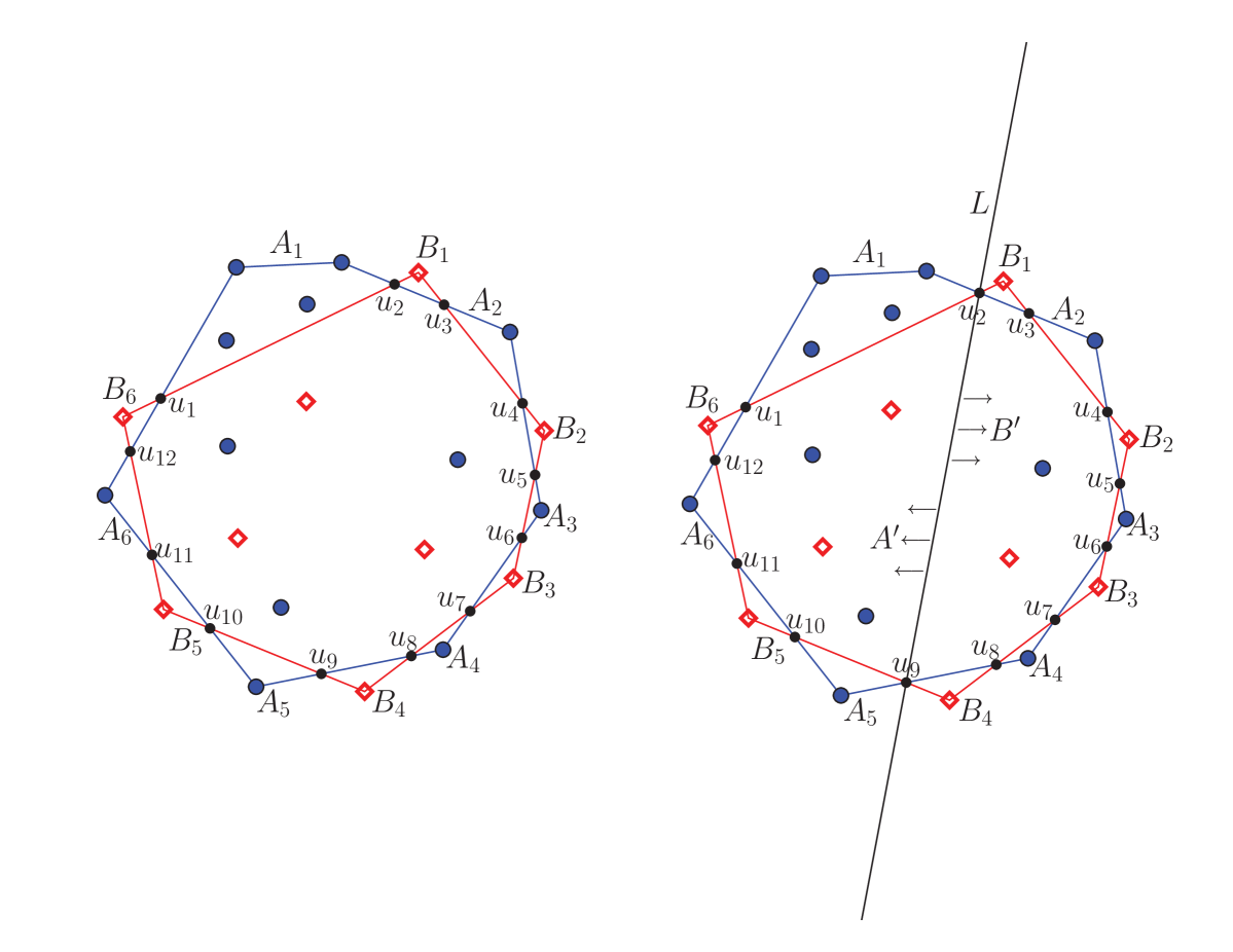
Figure 1. $A$ (blue points) and $B$ (red points) are not separable (left). $A\cup B$ can be split by $L$ into new subsets $A^{\prime}$ and $B^{\prime}$ without increase of the Euclidean diameters (right).

Lemma 2.2.

Let $(A_{i},B_{j})$ and $(A_{i^{\prime}},B_{j^{\prime}})$ be two bad pairs such that $A_{i}\neq A_{i^{\prime}}$ and $B_{j}\neq B_{j^{\prime}}$. Let us choose $a_{i}\in A_{i},b_{j}\in B_{j},a_{i^{\prime}}\in A_{i^{\prime}},b_{j^{\prime}}\in B_{j^{\prime}}$ such that $\overline{a_{i}b_{j}}$ and $\overline{a_{i^{\prime}}b_{j^{\prime}}}$ are bad segments. Then, either these bad segments intersect, or any point $a\in A_{m}$ belonging to the halfplane defined by $\langle b_{j}b_{j^{\prime}}\rangle$ where $a_{i}$ and $a_{i^{\prime}}$ are not contained, is not bad.

Proof.

Let us assume that $\overline{a_{i}b_{j}}$ and $\overline{a_{i^{\prime}}b_{j^{\prime}}}$ are bad segments with an empty intersection set. There are two cases (disregarding symmetric variations) for the relative positions of the points on the boundary of $\mathrm{conv}(\{a_{i},a_{i^{\prime}},b_{j},b_{j^{\prime}}\})$.

Case 1: $a_{i},b_{j^{\prime}},a_{i^{\prime}},b_{j}$ is the sequence of the points in clockwise order. Then, we get a contradiction:

$$\mathrm{diam}(A)+\mathrm{diam}(B)\geq\|a_{i}-a_{i^{\prime}}\|+\|b_{j}-b_{j^{\prime}}\|\geq\\ \|a_{i}-b_{j}\|+\|a_{i^{\prime}}-b_{j^{\prime}}\|>2\ \mathrm{diam}(A).$$

Case 2: $a_{i},a_{i^{\prime}},b_{j^{\prime}},b_{j}$ is the sequence of the points in clockwise order. Let us assume that there exists a bad segment $\overline{a_{m}b_{k}}$ such that $a_{m}\in A_{m}$ belonging to the halfplane defined by $\langle b_{j}b_{j^{\prime}}\rangle$ where $a_{i}$ and $a_{i^{\prime}}$ are not contained. The half-lines starting in $a_{m}$ and connecting $a_{m}$ with $a_{i}$ and with $a_{i^{\prime}}$, and the lines $\langle a_{m},b_{j}\rangle$ and $\langle a_{m},b_{j^{\prime}}\rangle$, divide the plane in six zones (see Figure 2).

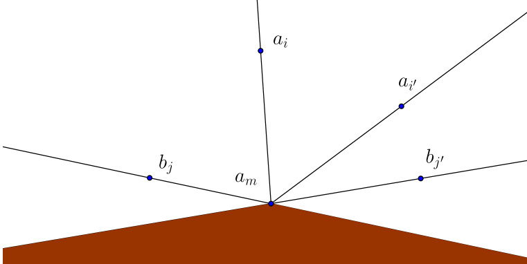
Figure 2. If $(a_{i},b_{j})$ and $(a_{i^{\prime}},b_{j^{\prime}})$ are bad partners, then the shaded zone can not contain a bad partner of $a_{m}\in A_{m}$

By convexity, one of these zones (the shaded zone in Figure 2) can not contain $b_{k}$. If $b_{k}$ belongs to whichever other zone, it is possible to consider a quadrangle whose vertices are situated in clockwise order like in Case 1, and we get a contradiction. Therefore, if this case holds, then $a_{m}$ is not a bad point. ∎

Remark 2.3:

Case 2 does not occur in $\mathbb{E}^{2}$, and as a consequence every two bad segments from disjoint bad pairs $(A_{i},B_{j})$ and $(A_{i^{\prime}},B_{j^{\prime}})$ cross. In order to prove this in [6], it is used the property that in an obtuse triangle the longest side is opposite to the obtuse angle. But if we consider the normed plane with unit sphere made by two arcs of circunferences showed in Figure 3, the triangle with vertices $a_{m},b,c,$ has an obtuse angle on vertix $a_{m}$, and the side $\overline{bc}$ is not the longest one. Besides, there is a configuration of points similar to Case 2 where $\overline{a_{i^{\prime}}b_{j^{\prime}}}$ and $\overline{a_{i}b_{j}}$ are non intersecting, and such that $\mathrm{min}\{\|a_{i}-b_{j}\|,\|a_{i^{\prime}}-b_{j^{\prime}}\|\}>\mathrm{diam}(\{a_{i},a_{i^{\prime}},a_{m}\})=1>\mathrm{diam}(\{b_{j},b_{j^{\prime}}\})$.

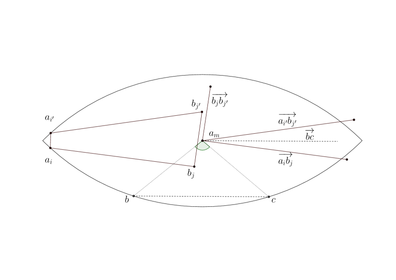
Figure 3. $\|b-c\|<\|a_{m}-b\|=\|a_{m}-c\|=1$ and                   $\|a_{i^{\prime}}-b_{j^{\prime}}\|>\|a_{i}-b_{j}\|>\mathrm{diam}(\{a_{i},a_{i^{\prime}},a_{m}\})>\mathrm{diam}(\{b_{j},b_{j^{\prime}}\})$.

Before splitting the sets $A$ and $B$, we group all the bad adjacent subsets $A_{i}$ from the cluster $A$. Namely, maximal cyclic groups of bad subsets $A_{i}$ are made. If $A_{i}$ and $A_{i^{\prime}}$ (clockwise order) are bad subsets belonging to the same group, then there is not any not bad $A_{k}$ between $A_{i}$ and $A_{i^{\prime}}$, although some not bad $B_{j}$ can be situated between $A_{i}$ and $A_{i^{\prime}}$. The same is made with cluster $B$. These maximal cyclic groups are noted by $\bar{A}_{1},\bar{A}_{2},\dots,\bar{A_{p}}$ and $\bar{B_{1}},\bar{B_{2}},\dots,\bar{B_{q}}$.

We say that $(\bar{A}_{i},\bar{B}_{j})$ is a bad pair of groups if there exits a bad segment from $\bar{A}_{i}$ to $\bar{B}_{j}$. Two pair of sets $(A_{i},B_{j})$ and $(A_{i^{\prime}},B_{j^{\prime}})$ cross if there exist two (one from every pair) bad-crossing segments. Similarly, $(\bar{A}_{i},\bar{B}_{j})$ and $(\bar{A}_{i^{\prime}},\bar{B}_{j^{\prime}})$ cross if there exist two (one from every pair) bad-crossing segments.

Lemma 2.4.

Let $(A_{i},B_{j})$ and $(A_{i^{\prime}},B_{j^{\prime}})$ be two bad pairs such that $A_{i}\neq A_{i^{\prime}}$ and $B_{j}\neq B_{j^{\prime}}$. If $A_{i}$ and $A_{i^{\prime}}$ belong to a group $\bar{A_{k}}$, then a group $\bar{B_{t}}$ contains $B_{j}$ and $B_{j^{\prime}}$.

Proof.

Let us assume that $(A_{i},B_{j})$ and $(A_{i^{\prime}},B_{j^{\prime}})$ are two bad pairs such that $A_{i}$ and $A_{i^{\prime}}$ belong to the same group, but $B_{j}$ and $B_{j^{\prime}}$ belong to different groups. Then it must exist a bad set $A_{m}$ between $B_{j}$ and $B_{j^{\prime}}$. Let $B_{k}$ be a bad partner of $A_{m}$. $(A_{i},B_{j})$ and $(A_{i^{\prime}},B_{j^{\prime}})$ must cross (if not, by Lemma 2.2, $A_{m}$ can not contain bad points). Since $A_{i}$ and $A_{i^{\prime}}$ belong to the same group, only one of them (not both) cross with $(A_{m},B_{k})$. Let us assume that $(A_{i},B_{j})$ and $(A_{m},B_{k})$ cross. There exist $a_{m}\in A_{m},b_{k}\in B_{k},a_{i^{\prime}}\in A_{i^{\prime}},b_{j^{\prime}}\in B_{j^{\prime}}$ that would be situated in an impossible clockwise order $a_{m},b_{k},a_{i^{\prime}},b_{j^{\prime}}$ (similar to Case 1 in Lemma 2.2), and we get a contradiction. ∎

Due to Lemma 2.4, the number of maximal cyclic groups for $A$ and for $B$ is the same.

Lemma 2.5.

Let $(\bar{A}_{i},\bar{B}_{j})$ and $(\bar{A}_{i^{\prime}},\bar{B}_{j^{\prime}})$ be two bad pair of groups such that $\bar{A}_{i}\neq\bar{A}_{i^{\prime}}$ and $\bar{B}_{j}\neq\bar{B}_{j^{\prime}}$. Then $(\bar{A}_{i},\bar{B}_{j})$ and $(\bar{A}_{i^{\prime}},\bar{B}_{j^{\prime}})$ cross.

Proof.

The clockwise order can not be $\bar{A}_{i},\bar{B}_{j^{\prime}},\bar{A}_{i^{\prime}},\bar{B}_{j}$ (due to the arguments used in Lemma 2.2, Case 1); and neither $\bar{A}_{i},\bar{A}_{i^{\prime}},\bar{B}_{j^{\prime}},\bar{B}_{j}$, because then $\bar{B}_{j^{\prime}}$ and $\bar{B}_{j}$ can not be separated by a bad polygon $A_{m}$ (Lemmma 2.2, Case 2). Therefore, the clockwise order must be $\bar{A}_{i},\bar{A}_{i^{\prime}},\bar{B}_{j},\bar{B}_{j^{\prime}}$, and the groups cross. ∎

And we obtain the following from Lemma 2.5.

Corollary 2.6.

There is an odd number of groups from each cluster, and they are completely interlacing.

Let $A_{i}$ be the last bad set of a group (in clockwise order), and let $B_{j^{\prime}}$ be the last bad partner of $A_{i}$. Let $B_{j}$ be the first bad set after $A_{i}$, and let $A_{i^{\prime}}$ be the first bad partner of $B_{j}$. We choose the separating line $L$ to go through the point $u_{2j}$ before $B_{j}$ and the point $u_{2j^{\prime}+1}$ after $B_{j^{\prime}}$ (see Figure 1). We define $B^{\prime}$ to be the points in $A\cup B$ lying on the same side of $L$ as $B_{j}$ and $B_{j^{\prime}}$, and $A^{\prime}$ as the remaining points.

Proposition 2.7.

The diameter of $A^{\prime}$ is less than or equal to the diameter of $A$.

Proof.

Since $L$ cuts all bad pairs, there does not exist a bad point $a^{\prime}\in A^{\prime}$ with a bad partner inside $A^{\prime}$ (the same happens with $B^{\prime}$), and the diameter of $A$ (and as well as the diameter of $B^{\prime}$) have length less than or equal to $\mathrm{diam}(A)$. ∎

Proposition 2.8.

The diameter of $B^{\prime}$ is less than or equal to the diameter of $B$.

Proof.

Let $a,b\in B^{\prime}$. We have to prove that $\|a-b\|\leq\mathrm{diam}(B).$ If $a,b\in B$ there is nothing to prove. In other case, let us assume that $\|a-b\|>\mathrm{diam}(B)$. Let us choose $a_{i}\in A_{i}$, $b_{j}\in B_{j}$, $a_{i^{\prime}}\in A_{i^{\prime}}$, $b_{j^{\prime}}\in B_{j^{\prime}}$ such that $(a_{i},b_{j^{\prime}})$ and $(a_{i^{\prime}},b_{j})$ are bad pairs. There are three possible cases.

Case 1: $a\in\mathrm{conv}(A)\setminus\mathrm{conv}(B)$ and $b\in\mathrm{conv}(B)\setminus\mathrm{conv}(A)$. The points $\{b_{j},a,b,b_{j^{\prime}},a_{i^{\prime}},a_{i}\}$ are situated around $\mathrm{conv}(A)\cap\mathrm{conv}(B)$ and it is possible to consider a clockwise order. If $\{a,b\}$ is the clockwise order of these two points, we observe the quadrangle with vertices (clockwise) $\{b_{j},a,b,a_{i^{\prime}}\}$ and the following contradiction holds:

(2.1) $$\mathrm{diam}(A)+\mathrm{diam}(B)\geq\|a-a_{i^{\prime}}\|+\|b-b_{j}\|\geq\\ \|b_{j}-a_{i^{\prime}}\|+\|a-b\|>\mathrm{diam}(A)+\mathrm{diam}(B).$$

If the clockwise order is $\{b,a\}$, we obtain a similar contradiction on the quadrangle with vertices (clockwise order) $\{a_{i},b,a,b_{j^{\prime}}\}$.

Case 2: $a,b\in\mathrm{conv}(A)\setminus\mathrm{conv}(B)$. Case 1 implies that $\|b-b^{\prime}\|\leq\mathrm{diam}(B)$ for every $b^{\prime}\in(\mathrm{conv}(B)\setminus\mathrm{conv}(A))\cap B^{\prime}$. If $\{a,b\}$ is the clockwise order of these two vertices, we can apply an argument similar to (2.1) to the quadrangle $\{b_{j},a,b,a_{i^{\prime}}\}$:

$$\mathrm{diam}(A)+\mathrm{diam}(B)\geq\|a-a_{i^{\prime}}\|+\|b-b_{j}\|\geq\\ \|b_{j}-a_{i^{\prime}}\|+\|a-b\|>\mathrm{diam}(A)+\mathrm{diam}(B),$$

which is again a contradiction. If the order is $\{b,a\}$, we use the quadrangle $\{b_{j},b,a,a_{i^{\prime}}\}$.

Case 3: $a\in\mathrm{conv}(A)\setminus\mathrm{conv}(B)$ and $b\in\mathrm{conv}(A)\cap\mathrm{conv}(B)$. Since the distance from $a$ is maximized at some vertex of $\mathrm{conv}(A)\cap\mathrm{conv}(B)\cap\mathrm{conv}(B^{\prime}),$ we may assume that $b$ is one of these vertices and apply an analysis similar to Case 1 or to Case 2. ∎

Using the previous results, we obtain the main theorem.

Theorem 2.9.

Let $A$ and $B$ be two sets of a finite number of points in $\mathbb{M}^{2}$. Then, there are two linearly separable sets $A^{\prime}$ and $B^{\prime}$ such that $\mathrm{diam}(A^{\prime})\leq\mathrm{diam}(A)$, $\mathrm{diam}(B^{\prime})\leq\mathrm{diam}(B)$, and $A^{\prime}\cup B^{\prime}=A\cup B.$

Corollary 2.10.

The construction in Theorem 2.9 verifies that

$$\mathrm{perimeter}(\mathrm{conv}(A))+\mathrm{perimeter}(\mathrm{conv}(B))\geq\\ \mathrm{perimeter}(\mathrm{conv}(A^{\prime}))+\mathrm{perimeter}(\mathrm{conv}(B^{\prime})).$$

If $\mathrm{conv}(A)\cap\mathrm{conv}($B$)\neq\emptyset$, then the inequality is strict.

Proof.

We note $\mathrm{p}(S)$ to the perimeter of a set $S$. If $\mathrm{conv}(A)\cap\mathrm{conv}(B)$ is a segment or the empty set, there is nothing to prove. Let us assume that $\mathrm{conv}(A)\cap\mathrm{conv}(B)\neq\emptyset$. We note $l$ to the length of $L\cap\mathrm{conv}(A)\cap\mathrm{conv}(B)$, where $L$ is the splitting line of bad pairs from $A^{\prime}$ and $B^{\prime}$ in Theorem 2.9. The following holds (see Figure 1):

$$\mathrm{p}(\mathrm{conv}(A^{\prime}))+\mathrm{p}(\mathrm{conv}(B^{\prime}))\leq\\ \sum_{i}\mathrm{p}(A_{i})+\sum_{j}\mathrm{p}(B_{j})-\mathrm{p}(\mathrm{conv}(A)\cap\mathrm{conv}(B))+2l<\\ \sum_{i}\mathrm{p}(A_{i})+\sum_{j}\mathrm{p}(B_{j})=\mathrm{p}(\mathrm{conv}(A))+\mathrm{p}(\mathrm{conv}(B))$$

∎

3. Some applications to clustering problems

From now on, $S$ is a set of $n$ points in a normed plane $\mathbb{M}^{2}$. We assume that in our computation model the unit ball of $\mathbb{M}^{2}$ is given via an oracle as it is described in Section 3.3 of [8] or on page 316 in [16].

3.1. 2-clustering problem: minimize the maximum diameter.

Given a metric, the $2$-clustering problem of minimizing the maximum diameter asks about how to split $S$ into two sets minimizing the maximum diameter. Avis solves the problem in $\mathbb{R}^{2}$ looking for two separable sets with the following algorithm ($O(n^{2}\log^{2}n)$ time).

 Algorithm 3.1

  Given a set $S$ of $n$ points in the plane:

1. Sort the distances $d_{i}$ between the points of $S$ into increasing order ($O(n^{2}\log n)$ time).

2. Locate the minimum $d_{i}$ that admits a stabbing line by a binary search. Use the graph $(S,E_{d_{i}})$, where $E_{d_{i}}$ is the set of edges meeting two points of $S$ at distance more than $d_{i}$, and the algorithm by Edelsbrunner et al. ([7]) in order to find the stabbing line for $E_{d_{i}}$ ($O(m\log m)$ time each) as a subroutine.

  We obtain the following from Theorem 2.9.

Corollary 3.1.

Given a set of $n$ points in $\mathbb{M}^{2}$, the $2$-clustering problem of minimizing the maximum diameter can be computed in $O(n^{2}\log^{2}n)$ time using Algorithm 3.1.

Asano et al. ([4]) reduce the cost of Algorithm 3.1 to $O(n\log n)$ time in $\mathbb{E}^{2}$. They use the maximum spanning tree of $S$ (that can be constructed in such a time and space in $\mathbb{E}^{2}$; see [17]) instead of all the distances between points of $S$. This approach also works correctly in $\mathbb{M}^{2}$, but as far as we know, there is not a similar result about the cost of building a maximum spanning tree for any normed plane.

3.2. 2-clustering problem: constraints over the diameters

Given $d_{1}\geq d_{2}>0$, Hershberger and Suri ([11]) solve in $\mathbb{E}^{2}$ the problem of dividing $S$ into two sets $S_{1}$ and $S_{2}$ such that $\operatorname{diam}(S_{1})\leq d_{1}$ and $\operatorname{diam}(S_{2})\leq d_{2}$ ($O(n\log n)$ time). They uses the fact that if $\|a-b\|\geq d_{1}$, then $B(a,d_{2})\cap B(b,d_{1})$ can always be split into two subsets whose diameters are at most $d_{1}$ and $d_{2}$, respectively. Nevertheless, the following example shows that this can not be extended to $\mathbb{M}^{2}$. Let us consider $a=(0,0)$, $b=(-9.81,6.24)$, and the strictly convex norm whose unit sphere is bounded by the two arcs of circles with center in $(0,10)$ and in $(0,-10)$, respectively, and radius $5\sqrt{13}$ (see Figure 4). Let $\{r=(r_{1},r_{2}),\quad s=(s_{1},s_{2})\}\in S(a,1)$ and $\{p,q\}=S(a,1)\cap S(b,1.1)$, such that $r_{1}=-9.39$, $r_{2}>0$, $s_{1}=-8.24$, $s_{2}>0$, and $p,r,s,q$ is the clockwise order on $S(a,1)$. It is verified that $\|a-b\|\geq 1.1$, $\mathrm{min}\{\|s-p\|,\|r-q\|,\|p-q\|\}>1.1$ and $\mathrm{min}\{\|r-p\|,\|s-q\|\}>1$. Therefore the set $S=\{p,q,r,s\}\in B(a,1)\cap B(b,1.1)$ can not be divided in two subsets whose diameters are at most $1.1$ and $1$, respectively.

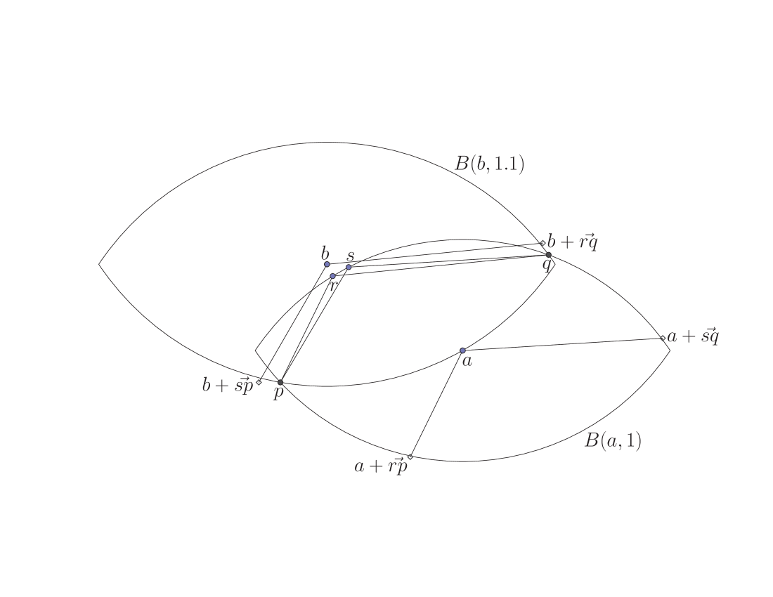
Figure 4. $S=\{p,q,r,s\}$ can not be divided in two subsets with diameters less than or equal to $1.1$ and $1$, respectively.

However we can look for a separable pair of sets $S_{1}$ and $S_{2}$.

Corollary 3.2.

Given a set $S$ of $n$ points in $\mathbb{M}^{2}$, and $d_{1}\geq d_{2}>0$, the $2$-clustering problem of dividing $S$ into two sets $S_{1}$ and $S_{2}$ such that $\operatorname{diam}(S_{1})\leq d_{1}$ and $\operatorname{diam}(S_{2})\leq d_{2}$ can be solved in $O(n^{2}\log n)$ time.

Proof.

Let $E_{d_{1}}$ be the set of edges meeting two points of $S$ at distance more than $d_{1}$. Sort the distances between the points of $S$ into increasing order and build the graph $(S,E_{d_{1}})$ in $O(n^{2}\log n)$ time. Test if $E_{d_{1}}$ has a stabbing line (in $O(n\log n)$ time with the algorithm presented in [7]). If the stabbing line does not exist, there is no solution (Theorem 2.9). If the stabbing line exists, check if one of the subsets of $S$ separated by the the stabbing line has diameter less than or equal to $d_{2}$. ∎

3.3. $k$-clustering problems

The $k$-clustering problem of minimizing the maximum diameter is the natural extension of the case $k=2$ presented in Section 3.1. It is a particular case of the $k$-clustering problem of minimizing $\mathcal{F}$ over the diameters, where $\mathcal{F}$ is a monotone increasing function $\mathcal{F}:\mathbb{R}^{k}\rightarrow\mathbb{R}$ that is applied over the diameters of the clusters (for instance, $\mathcal{F}$ can be the maximum, the sum, or the sum of squares of the diameters). If we consider the radii instead of the diameters, we talk about the $k$-clustering problem of minimizing $\mathcal{F}$ over the radii.

The following result is presented in [6] for the Euclidean subcase.

Theorem 3.3.

Let $S$ be a set of $n$ points in $\mathbb{M}^{2}$. Consider the $k$-clustering problem of minimizing a monotone increasing function $\mathcal{F}:\mathbb{R}^{k}\rightarrow\mathbb{R}$ that is applied over the diameters or over the radii of $k$ subsets of $S$. Then there is an optimal $k$-clustering such that each pair of clusters is linearly separable.

Proof.

Regarding the diameter, let us consider an optimal solution of the problem that minimizes the sum of the $k$ perimeters of the convex hulls of the clusters. Theorem 2.9 and Corollary 2.10 imply that there exist a $k$-clustering (with smaller or equal sum of perimeters) such that every pair of clusters are separable, and the value of $\mathcal{F}$ does not increase.

Let us consider now the $k$-clustering problem of minimizing $\mathcal{F}$ over the radii. Let $C_{1}$ and $C_{2}$ be two clusters of $S$ from an optimal solution, and $B(u,r)$ and $B(v,r^{\prime})$ be two minimal enclosing discs of $C_{1}$ and $C_{2}$, respectively, such that $C_{1}\subset B(u,r)$ and $C_{2}\subset B(v,r^{\prime})$. If $S(u,r)\cap S(v,r^{\prime})$ is the empty set or has only one connected component, $C_{1}$ and $C_{2}$ are separable. If $S(u,r)\cap S(v,r^{\prime})$ has two different components $A_{1}$ and $A_{2}$, we consider a line $L$ meeting two points $p_{1}\in A_{1}$ and $p_{2}\in A_{2}$. Let $u_{i}=p_{i}-(v-u)$ and $v_{i}=p_{i}+(v-u)$ for $i=1,2.$ Let $S_{1}(u,r)$ be the part of $S(u,r)$ on the same side of the line $\langle p_{1},p_{2}\rangle$ as $u_{1}$ and $u_{2}$; let $S_{2}(u,r)$ be the part of $S(u,r)$ on the side of $\langle p_{1},p_{2}\rangle$ opposite to $u_{1}$ and $u_{2}$. Let $S_{1}(v,r^{\prime})$ be the part of $S(v,r^{\prime})$ on the same side of the line $\langle p_{1},p_{2}\rangle$ as $v_{1}$ and $v_{2}$; let $S_{2}(v,r^{\prime})$ be the part of $S(v,r^{\prime})$ on the side of $\langle p_{1},p_{2}\rangle$ opposite to $v_{1}$ and $v_{2}$. Then, $S_{2}(u,r)\subseteq\operatorname{conv}(S_{1}(v,r^{\prime}))$ and $S_{2}(v,r^{\prime})\subseteq\operatorname{conv}(S_{1}(u,r))$ (see Grünbaum [9] and Banasiak [5]). The subsets $S\cap\operatorname{conv}(S_{1}(u,r))$ and $S\cap\operatorname{conv}(S_{1}(v,r^{\prime}))$ are two separable clusters, and the minimal enclosing radius of the new clusters are no greater.

Consequently we can reassign the points for every pair of intersecting clusters according to their position relative to the line $L$. Finally we obtain a $k$-clustering such that every two clusters are separable and the value of $\mathcal{F}$ does not increase. ∎

Therefore the optimal solution for the $k$-clustering problem of minimizing $\mathcal{F}$ over the diameter or over the radius is a planar dissection into $k$ convex polygonal regions, such that each of them contains a cluster $C_{i}$. It can be represented by a graph $G=(V,E)$, where every vertex $v_{i}\in V$ corresponds to the region of a cluster $C_{i}$, and every edge $\{ij\}$ joints $v_{i}$ and $v_{j}$ if and only if a common boundary separates the polygonal regions that contain $C_{i}$ and $C_{j}$. The following algorithm by Capoyleas et al. ([6]) solves the $k$-clustering problem of minimizing a monotone increasing function $\mathcal{F}$ over the diameters or over the radii in the Euclidean plane.

 Algorithm 3.2

  Given a set $S$ of $n$ points in the plane:

1. For every graph (up to isometric ones) $G=\{V,E\}$ with $k$ vertices do the following:

2. For every edge $\{ij\}\in E$, select a line and specify which side $H_{ij}$ of this line is to contain $C_{i}$ and which side $H_{ji}$ should contain $C_{j}$.

3. For each point $p\in S$, determine to which side it belongs, and then for each $i$ evaluate

   $$R_{i}^{\prime}=\bigcap_{\{ij\}\in E}H_{ij}$$

   Every region $R_{i}^{\prime}$ contains $C_{i}$, and they are pairwise disjoint (see Lemma 8 in [6]). If each point happens to fall into exactly one cluster, we have a candidate for an optimal solution.

4. Evaluate the diameter (or the radius) of every cluster $C_{i}$, and then the function $\mathcal{F}$.

5. Take the minimum of the values of $\mathcal{F}$.

 

Corollary 3.4.

Let $S$ be a set of $n$ points in $\mathbb{M}^{2}$. For any fixed $k$, the geometric $k$-clustering problem of minimizing a monotone increasing function $\mathcal{F}$ over the diameters or over the radii is solvable by Algorithm 3.3. It takes polynomial time for the diameter.

Proof.

By Theorem 3.3, Algorithm 3.3 (see Lemma 8 and Theorem 9 in [6] for details) works correctly in $\mathbb{M}^{2}$ too.

The number of non-isometric graphs with $k$ vertices is fixed. The number of edges is at most $3k-6$, and $n$ points can be separated by these edges in $O(n^{6k-12})$ different ways. Regarding step (4) of Algorithm 3.3, the diameter of a set of $n$ points can be computed in $O(n\log n)$ time in $\mathbb{M}^{2}$ with the same algorithm that in $\mathbb{E}^{2}$ ([18]). Therefore, the $k$-clustering problem for minimizing the diameter in $\mathbb{M}^{2}$ is solvable in polynomial time. ∎

It seems that there is not an optimal solution for determining the minimal enclosing radius of a set of points in $\mathbb{M}^{2}$. Two algorithms are presented in [12] for strictly convex normed planes. The first one is similar to Elzinga/Hearn’s and takes $\Omega(n^{2})$ time. The other is similar to Shamos/Hoey’s and enables an $O(n)$ search for the optimal disk once the farthest-point Voronoi diagram of the set is constructed. Nevertheless, the strictly convex case can be solved by an easier way because the radius and the covering circle of each cluster are determined by at most three points ([1], [2]). Hence it would be enough to check only $O(n^{3k})$ possibilities.

3.4. $3$-clustering problems

Having in mind Theorem 3.3, we can do the following in order to solve the $3$-clustering problem minimizing the maximum diameter: (1) Separate the $n$ points in all possible two linear separable sets ($O(n^{4})$ possibilities); (2) Use Algortihm 3.1 to split the second of these sets; (3) Determine the optimal solution. This takes $O(n^{6}\log^{2}n)$ time if Avis’ approach is used, and it could be improved with the algorithm by Asano et al. But we prove in this section that Hauger-Rote’s $3$-clustering approach for $\mathbb{E}^{2}$ ([10]) works correctly in $\mathbb{M}^{2}$ with some modifications.

We fix a normal basis $\{x,y\}$ in $\mathbb{M}^{2}$ such that $x$ is Birkhoff orthogonal to $y$ (namely, such that $\|x\|\leq\|x+\lambda y\|$ for every $\lambda\in\mathbb{R}$). It is assumed that two given points of $S$ have different $x$ and $y$ coordinate (the points are rotated if it is necessary). Given $d>0$, the algorithm searches all the possible linearly separable subsets $A,B,C,$ such that the maximum diameter is less than or equal to $d$. The point $a\in S$ with minimum $x$-coordinate is placed in $A$, and each point $a^{\prime}\in S$ such as $\|a-a^{\prime}\|\leq d$ is tested as the possible point of $A$ with the maximum $x$-coordinate. Any $u\in S\cap\overline{aa^{\prime}}$ is assing to $A.$ The plane is divided in the following three zones by the lines $\langle a,a^{\prime}\rangle$ and $a^{\prime}+\beta y$ ($\beta\in\mathbb{R}$):

$$\begin{array}[]{ll}\textsc{North}:=&\{u\in S/\;u=\alpha a+(1-\alpha)a^{\prime}+\beta y,\text{ with }1>\alpha>0,\beta>0\}\\ \textsc{{South}}:=&\{u\in S/\;u=\alpha a+(1-\alpha)a^{\prime}+\beta y,\text{ with }1>\alpha>0,\beta<0\}\\ \textsc{{East}}:=&\{u\in S/\;u=-\alpha a+(1+\alpha)a^{\prime}+\beta y,\text{ with }\alpha>1\}\\ \end{array}$$

There is not any point of $S$ on the ”left” of $a+\beta y$ ($\beta\in\mathbb{R}$). East contains the points of $S$ on the ”right” of the line $a^{\prime}+\beta y$. The points of $S$ on the left of $a^{\prime}+\beta y$ are contained either in North (if they are ”above” $\overline{aa^{\prime}}$) or in South (if they are ”bellow” $\overline{aa^{\prime}}$).

Solutions are tested in three different cases: Case 1, $\text{{North}}\subseteq A$; Case 2, $\text{{South}}\subseteq A$; and Case 3, North and South are not completely contained in $A$. We note $A_{cand}$ to the set of points that could be placed in $A$ for every candidate $a^{\prime}$:

$$A_{cand}=S\cap B(a,d)\cap B(a^{\prime},d).$$

Lemma 3.5.

With the previous notations, the following holds in $\mathbb{M}^{2}$:

$$\operatorname{diam}(A_{cand}\cap\operatorname{\textsc{North}})\leq d\hskip 8.5359pt\text{and}\hskip 8.5359pt\operatorname{diam}(A_{cand}\cap\operatorname{\textsc{South}})\leq d.$$

Proof.

Proposition 1(iii) in [6] for $\mathbb{E}^{2}$ can be applied for $\mathbb{M}^{2}$: due to the geometry of the figure, $\mathrm{diam}(A_{cand}\cap\operatorname{\textsc{{North}}})$ is equal to the distance between two support lines, and one of them has to pass through $a$ or $a^{\prime}$. Since all the points are within $B(a,d)\cap B(a^{\prime},d)$, the diameter is at most $d$. Similarly for $\mathrm{diam}(A_{cand}\cap\operatorname{\textsc{{South}}})$. ∎

Lemma 3.6.

Let us assume the following conditions in $\mathbb{M}^{2}$:

• $\max\{\operatorname{diam}(A),\operatorname{diam}(B),\operatorname{diam}(C)\}\leq d$,

• $A,B,C$ are separable,

• $B\cap\text{{North}}\neq\varnothing$ and $C\cap\text{{{South}}}\neq\varnothing.$

If there exist a pair of points $u=(u_{x},u_{y}),v=(v_{x},v_{y})\in\text{{East}}$ such that $\|u-v\|>d$ and $u_{y}>v_{y}$, then $u\in B$ and $v\in C.$

Proof.

Since $\|u-v\|>d$, the points $u$ and $v$ can not be situated in the same subset of the partition $A,B,C$. We can choose $u^{\prime}=(u^{\prime}_{x},u^{\prime}_{y})\in B\cap\text{{North}}$ and $v^{\prime}=(v^{\prime}_{x},v^{\prime}_{y})\in C\cap\text{{South}}$.

Let us assume that $u_{y}>v^{\prime}_{y}$. If $v$ is situated in the shaded zone in Figure 5, $v$ must belong to $C$, because in other case either the pair of segments $\overline{vu^{\prime}}$ and $\overline{uv^{\prime}}$ or the pair of the segments $\overline{vu^{\prime}}$ and $\overline{aa^{\prime}}$ cross.

If $v$ is not situated in the shaded zone in Figure 5 and $u_{x}<v_{x}$ (for instance, $v=v_{1}$ in Figure 5), we consider the two intersection points of the line $u+\lambda y$ with the line $v+\lambda x$ and with the line $v+\lambda(u^{\prime}-v)$, that we note by $\bar{u}$ and $\widetilde{u}$, respectively. Since $x$ is Birkhoff orthogonal to $y$, $u+\lambda y$ supports $S(v,\|\bar{u}-v\|)$ on $\bar{u}$, and $\|v-u^{\prime}\|\geq\|v-\widetilde{u}\|\geq\|v-u\|\geq\|v-\bar{u}\|$. As a result of $\|v-u^{\prime}\|\geq\|v-u\|>d$, $v\in C$.

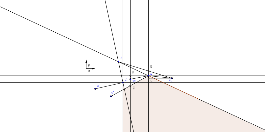
Figure 5.

If $v$ is not situated in the shaded zone in Figure 5 and $u_{x}>v_{x}$ (for instance, $v=v_{2}$ in Figure 5), we consider the two intersection points of the line $v+\lambda y$ with the line $u+\lambda x$ and with the line $u+\lambda(u-v^{\prime})$, that we note by $\bar{v}$ and $\widetilde{v}$, respectively. Since $x$ is Birkhoff orthogonal to $y$, the line $v+\lambda y$ is the support line of $S(u,\|u-\bar{v}\|)$ on $\bar{v}$, and $\|u-v^{\prime}\|\geq\|u-\widetilde{v}\|\geq\|u-v\|\geq\|u-\bar{v}\|$. As a result of $\|u-v^{\prime}\|\geq\|u-v\|>d$, $u\in B$.

The analysis is similar if $u_{y}<v^{\prime}_{y}$. ∎

The algorithm of Hagauer and Rote works in the following way.

 Algorithm 3.3

  Fix $a$ with the minimum $x$-coordinate. Then, for every $a^{\prime}\in S$:

1. Calculate North, South and East ($O(n)$ time).

2. Test Case 1 ($\text{{North}}\subseteq A$). Note $H=\{a,a^{\prime},\mathrm{\textsc{North}}\}$ and check if $\mathrm{diam}(H)\leq d$ ($O(n\log n)$ time). If yes, define

   $$A:=H\cup\left(\mathrm{\textsc{South}}\cap\big{(}\cap_{x\in H}B(x,d)\big{)}\right),$$

   Obtain $B$ and $C$ solving a $2$-clustering problem for the set $S\setminus A$ (for instance, in $O(n^{2}\log^{2}n)$ time by Algorithm 3.1).

3. Test Case 2 and manage it in a similar way as Case 1 ($O(n^{2}\log^{2}n)$ time).

4. Test Case 3 (neither North nor South are completely contained in $A$). Assign the points of $S$ that are initially forced to be in $A,B,C$ (by Lemma 3.6 and the rest of conditions) to the initial sets $A_{0},B_{0},C_{0}$:
   $\begin{array}[]{ll}A_{0}:=&\{a,a^{\prime}\}\\ B_{0}:=&\{u\in\mathrm{\textsc{North}}/\;u\notin\cap_{x\in A_{0}}B(x,d)\}\\ &\cup\{u\in\mathrm{\textsc{East}}/\;\exists v\in\mathrm{\textsc{East}},\|u-v\|>d,u_{y}>v_{y}\}\\ C_{0}:=&\{u\in\mathrm{\textsc{South}}/\;u\notin\cap_{x\in A_{0}}B(x,d)\}\\ &\cup\{u\in\mathrm{\textsc{East}}/\;\exists v\in\mathrm{\textsc{East}},\|u-v\|>d,u_{y}<v_{y}\},\end{array}$
   and the rest of the points of $S$ to one of the following candidate sets:
   $\begin{array}[]{ll}AB_{cand}:=&\mathrm{\textsc{North}}\setminus B_{0}\\ CA_{cand}:=&\mathrm{\textsc{{South}}}\setminus C_{0}\\ BC_{cand}:=&\mathrm{\textsc{East}}\setminus({B_{0}\cup C_{0}}).\end{array}$
   Stop if $B_{0}$ and $C_{0}$ are not disjoint (there is not a solution by Lemma 3.6). In other case, assign the points of the candidate sets to $A,B,C$ by Hauger and Rote’s procedure distribute (see [10]).

 

The set $A$ defined in Case 1 (as well as in Case 2) is the uniquely maximal feasible set with diameter less than or equal to $d$ (Lemma 3.5). The procedure distribute does not depend on the metric, therefore one solution is found in Case 3 (if there exists).

In order to implement the algorithm in $\mathbb{E}^{2}$, Hauger and Rote use the $d$-ball hull (also called $d$-circular hull) of a set $S$, and the data structure introduced by Hershberger and Suri ([11]). We justify in the Appendix that this data structure can be used in $\mathbb{M}^{2}$ (see Proposition 3.12).

Theorem 3.7.

Given a set of $n$ points in $\mathbb{M}^{2}$ and $d>0$, we can determine with the Algorithm 3.6 whether there is a partition of $S$ into sets $A,B,C$ with diameters at most $d$. This can be done in $O(n^{3}\log^{2}n)$ time.

Proof.

Hagauer-Rote’s proof (for $\mathbb{E}^{2}$) of the first part of statement depends on some lemmas (see Lemma 3 to Lemma 6 in [10]) and on Theorem 2.1. Once Theorem 2.1, and Lemma 3 and Lemma 4 in [10] are extended to $\mathbb{M}^{2}$ by our Theorem 2.9, Lemma 3.5 and Lemma 3.6, respectively, the rest of the lemmas and proofs can be applied to any normed plane. Regarding the complexity of the algorithm, the Hershberger and Suri’s data structure can be managed (see Proposition 3.12 in Appendix). Hence, for every $a^{\prime}\in S$ Case 1 and Case 2 take $O(n^{2}\log^{2}n)$ time (using Algorithm 3.1 as a subroutine), and Case 3 takes $O(n\log n)$ time as in $\mathbb{E}^{2}$ (see [10] for details). Therefore, the $3$-clustering algorithm takes $O(n^{3}\log^{2}n)$ time. ∎

Finally, a binary search on the ${n\choose 2}$ distances occurring in $S$ combined with Theorem 3.7 solves the optimization problem.

Theorem 3.8.

Given a set of $n$ points in $\mathbb{M}^{2}$, we can construct in $O(n^{3}\log^{3}n)$ time a partition of $S$ into sets $A,B,C$ such that the largest of the three dia-meters is as small as possible.

Appendix

Given a set $S$ in $\mathbb{M}^{2}$ and $d>0$, the $d$-ball hull $\operatorname{bh}(S,d)$ of $S$ (also called $d$-circular hull) is the intersection of all the balls of radius $d$ and center $x\in\mathbb{M}^{2}$ that contain $S$:

$$\operatorname{bh}(S,d)=\bigcap_{S\subseteq B(x,d)}B(x,d).$$

The data structure introduced by Hershberger and Suri ([11]) orders the points of the input set $S$ by their $x$-coordinates, and situates them on the leaves of a complete binary tree $T(S)$. Every node of $T(S)$ represents the $d$-ball hull of the points in the leaves of its subtree. Therefore, the root of $T(S)$ represents the $d$-ball hull of $S$. The information about every node is stored like a doubly linked list of its vertices such that for every vertex the predecessor and the successor is known. Since a point can be the vertex of more than one ball hull, for economizing space every point is only stored as vertex at the highest level in the tree at which it appears on a ball hull. It is proved ([11], see Lemma 4.1 to Lemma 4.16, and Theorem 4.17) that the data structure $T(S)$ (therefore the ball hull of $S$) can be built initially in $O(n\log n)$ time and it supports the following operations $(1)$ and $(2)$ in $\mathbb{E}^{2}$:

1. Given a query point $u\in S$, determine in $O(\log n)$ a point $v\in S$ such that $\|u-v\|\geq d$, if such a point exists.

2. It can be updated after a point deletion in $O(\log n)$ time.

The intersection of two spheres in $\mathbb{M}^{2}$ is always the union of two segments, each of which may degenerate to a point or to the empty set ([9], [5]; see also [15, $\S$ 3.3]). As a consequence, it is obtained the following ([14]).

Lemma 3.9.

Given $d>0$, for every pair of points $p,q\in\mathbb{M}^{2}$ whose distance is less than or equal to $2d$, there exist two circular arcs of radius $d$ meeting them (eventually only one, if they degenerate to the same segment) which belong to every disc of radius $d$ containing $p$ and $q$. These two arcs (if they are really two) are situated in different half planes bounded by the line $\langle p,q\rangle$. The center of each disc defining these two minimal arcs is an extreme points of the segments $S(p,d)\cap S(q,d)$.

We call $d$-minimal arc meeting $p$ and $q$ to each of these arcs cited in Lemma 3.9.

Lemma 3.10.

Given $d^{\prime}\geq d>0$, every ball of radius $d$ in $\mathbb{M}^{2}$ contains every $d^{\prime}$-minimal arc meeting two points of the ball.

Proof.

Let us consider $p,q\in B(u,d)$ for some $u\in\mathbb{M}^{2}.$ For every $r>0$, the $r$-ball hull of the set $\{p,q\}$ is the set bounded by the two $r$-minimal arcs meeting $p$ and $q$ (Lemma 3.9). Since the ball hull operator is decreasing with respect to the radius ([13]), then $\mathrm{bh}(\{p,q\},d^{\prime})\subseteq\mathrm{bh}(\{p,q\},d)$ and the statements holds. ∎

The following lemma ([14]) describes the geometry of the ball hull of a finite set in $\mathbb{M}^{2}$, and it is very similar to the Euclidean subcase.

Lemma 3.11.

Let $S=\{p_{1},p_{2},\dots,p_{n}\}$ be a finite set in $\mathbb{M}^{2}$. Then

$$\operatorname{bh}(S,d)=\bigcap_{S\subset B(x_{s},d)}B(x_{s},d)=\operatorname{conv}(\bigcup_{i,j=1}^{n}\widehat{p_{i}p_{j}}),$$

where $x_{s}$ are some extreme points of the components $S(p_{i},d)\cap S(p_{j},d)$, and $\widehat{p_{i}p_{j}}$ are $d$-minimal arcs meeting points of $S$ and whose centers are these extreme points $x_{s}$.

All the proofs from Lemma 4.1 to Lemma 4.16 and Theorem 4.17 in [11] can be extended almost word by word to $\mathbb{M}^{2}$ using the notion of minimal arc and Lemmas 3.9 to 3.11. As a consequence, Hershberger and Suri’s data structure works in a normed plane as does in $\mathbb{E}^{2}$.

Proposition 3.12.

The structure for managing ball hulls in $\mathbb{E}^{2}$ described by Hershberger and Suri works correctly in $\mathbb{M}^{2}$ and with the same time cost. It can be built initially in $O(n\log n)$ and supports the following operation:

1. Given a query point $u\in S$, determine in $O(\log n)$ a point $v\in S$ such that $\|u-v\|\geq d$, if such a point exists.

2. It can be updated after a point deletion in $O(\log n)$ time.

References

- [1] J. Alonso, H. Martini, and M. Spirova, Minimal enclosing discs, circumcircles, and circumcenters in normed planes (Part I), Comput. Geom. 45 (2012), 258-274.
- [2] J. Alonso, H. Martini, and M. Spirova, Minimal enclosing discs, circumcircles, and circumcenters in normed planes (Part II), Comput. Geom. 45 (2012), 350-369.
- [3] D. Avis, Diameter partitioning, Discrete Comput. Geom. 1 (1986), 265-276.
- [4] T. Asano, B. Bhattacharya, M. Keil, and F. Yao, Clustering algorithms based on minimum and maximum spanning trees, in Proc. 4th ACM Symposium on Computational Geometry, (1988), 252-257.
- [5] J. Banasiak, Some contributions to the geometry of normed linear spaces, Math. Nachr. 139 (1988), 175-184.
- [6] V. Capoyleas, G. Rote, and G. Woeginger, Geometric clustering, J. Algorithms 12 (1991), 341-356.
- [7] H. Edelsbrunner, H.A. Mauer, F.P. Preparata, A.L. Rosenberg, E. Welzl, and D. Wood, Stabbing line segments, BIT 22 (1982), 274-281.
- [8] P. Gritzmann, and V.L. Klee, On the complexity of some basic problems in computational convexity: I. Containment problems, Discrete Math. 136 (1994), 129-174.
- [9] B. Grünbaum, Borsuk’s partition conjecture in Minkowski planes, Bull. Res. Council Israel, Sect. F 7F (1957/1958), 25-30.
- [10] J. Hagauer, and G. Rote, Three-clustering of points in the plane, Comput. Geom. 8 (1997), 87-95.
- [11] J. Hershberger, and S. Suri, Finding tailored partitions, J. Algorithms 12 (1991), 431–463.
- [12] T. Jahn, Geometric algorithms for minimal enclosing discs in strictly convex normed planes, http://arxiv.org/abs/1410.4725
- [13] P. Martín, H. Martini, and M. Spirova, Chebyshev sets and ball operators, J. Convex Anal. 21 (2014), 601-618.
- [14] P. Martín, and H. Martini, Algorithms for ball hulls and ball intersections in normed planes, Journal of Computational Geometry 6 (2015), 99-107.
- [15] H. Martini, K.J. Swanepoel, and G. Weiss, The geometry of Minkowski spaces - a survey, Part I, Expositiones Math. 19 (2001), 97-142.
- [16] J. Matoušek, Lectures on Discrete Geometry, Graduate Texts in Mathematics, 212, Springer, New York, 2002.
- [17] C. Monma, M. Paterson, S. Suri, and F. Yao, Computing Euclidean maximum spanning trees, Algorithmica 5 (1990), 407-419.
- [18] F.P. Preparata, and M.I. Shamos, Computational Geometry, Springer-Verlag, New York, 1985.