Strong magnetic fields in nonlocal chiral quark models

Abstract

We study the behavior of strongly interacting matter under a uniform intense external magnetic field in the context of nonlocal extensions of the Polyakov$-$Nambu$-$Jona-Lasinio model. A detailed description of the formalism is presented, considering the cases of zero and finite temperature. In particular, we analyze the effect of the magnetic field on the chiral restoration and deconfinement transitions, which are found to occur at approximately the same critical temperatures. Our results show that these models offer a natural framework to account for the phenomenon of inverse magnetic catalysis found in lattice QCD calculations.

I Introduction

The study of the behavior of strongly interacting matter under intense external magnetic fields has gained increasing interest in the last few years. In fact, this topic has important applications e.g. in the description of compact objects like magnetars duncan , the analysis of heavy ion collisions at very high energies HIC and the exploration of the first phases of the Universe cosmo . Since these studies require dealing with QCD in nonperturbative regimes, present theoretical analyses are based either in the predictions of effective models or in the results obtained through lattice QCD (LQCD) calculations. In particular, the features of QCD phase transitions under external magnetic fields deserve significant interest. Recent reviews on this subject can be found in Refs. Kharzeev:2012ph ; Andersen:2014xxa ; Miransky:2015ava . In view of the difficulty of theoretical calculations, most works concentrate on the case in which one has a uniform and static external magnetic field $\vec{B}$. At zero temperature and chemical potential, both the results of low-energy effective models of QCD and LQCD calculations indicate that the chiral quark condensate should behave as an increasing function of $B$, which is usually known as “magnetic catalysis”. On the contrary, close to the chiral restoration temperature, LQCD calculations carried out with realistic quark masses Bali:2011qj ; Bali:2012zg show that light quark-antiquark condensates behave as nonmonotonic functions of the external magnetic field, and this leads to a decrease of the transition temperature when the magnetic field is increased. This effect is known as “inverse magnetic catalysis” (IMC). In addition, LQCD calculations predict an entanglement between the chiral restoration and deconfinement critical temperatures Bali:2011qj . These findings become a challenge to model calculations. Indeed, most naive effective approaches to low-energy QCD (Nambu$-$Jona-Lasinio model, chiral perturbation theory, MIT bag model, quark-meson models) predict that the chiral transition temperature should grow with $B$, i.e., they do not find IMC. In view of this discrepancy, in the last few years, some more sophisticated low-energy effective models compatible with the IMC effect have been proposed in the literature Skokov:2011ib ; Fraga:2012ev ; Bruckmann:2013oba ; Bali:2013esa ; Fukushima:2012kc ; Chao:2013qpa ; Fraga:2013ova ; Ferreira:2013tba ; Ferreira:2014kpa ; Ayala:2014iba ; Farias:2014eca ; Ayala:2014gwa ; Fayazbakhsh:2014mca ; Andersen:2014oaa ; Mueller:2015fka ; Ayala:2014uua ; Ferrer:2014qka ; Braun:2014fua ; Ruggieri:2014bqa ; Rougemont:2015oea ; Ayala:2015bgv ; Mao:2016fha . Possible mechanisms that allow the reproduction of IMC include, e.g., the introduction of adequate ($B$-dependent) regularization prescriptions, or explicit dependences of the effective coupling constants on the external field. In particular, in the framework of the Nambu$-$Jona-Lasinio (NJL) model, it has been shown that IMC can be obtained by considering a $B$-dependent four-fermion coupling Ayala:2014iba ; Farias:2014eca . On the other hand, the problem of the entanglement between the deconfinement and chiral restoration transitions has been studied in the context of the Polyakov$-$Nambu$-$Jona-Lasinio (PNJL) model, in which fermions are coupled to a background color field, and the traced Polyakov loop $\Phi$ is taken as order parameter of the confinement/deconfinement transition. This extension of the NJL model provides not only a description of confinement but also allows one to obtain chiral restoration critical temperatures compatible with those found in LQCD. In this framework, the effect of an external magnetic field has been studied in Ref. Gatto:2010pt , where the authors consider a Polyakov loop-dependent effective coupling constant in order to avoid the splitting between chiral restoration and deconfinement transitions. In this so-called “entangled PNJL” model, however, no IMC effect is found (see also Refs. Gatto:2012sp ; Ferreira:2013tba ). Once again, as shown in Ref. Ferreira:2014kpa , in the context of the PNJL model one can reproduce lattice IMC results by considering a $B$-dependent four-fermion coupling. Nevertheless, the results obtained in Ref. Ferreira:2014kpa lead to a relatively large splitting ($\gtrsim 30$ MeV) between chiral restoration and deconfinement temperatures.

In this work we study the behavior of strongly interacting matter under a uniform, static magnetic field in the framework of nonlocal chiral quark models. This article is an extension of a previous work in which it has been noticed that these kind of models offer a natural mechanism to understand the IMC effect Pagura:2016pwr . Our aim is to present here a more complete description of the formalism and also to extend the model to incorporate the interaction with the Polyakov loop. As in the case of the (local) NJL model, the traced Polyakov loop can be taken as an order parameter of confinement, allowing one to describe simultaneously the chiral restoration and deconfinement transitions. We will show that nonlocal models are able to describe, at the mean field level, not only the IMC effect but also the entanglement between both critical transition temperatures, in quite reasonable agreement with LQCD results. The “nonlocal PNJL” (nlPNJL) models considered here are a sort of nonlocal extensions of the PNJL model that intend to provide a more realistic effective approach to QCD. In fact, nonlocality arises naturally in the context of successful descriptions of low-energy quark dynamics Schafer:1996wv ; RW94 , and it has been shown Noguera:2008 that nonlocal models can lead to a momentum dependence in quark propagators that is consistent with LQCD results. It is also found that in this framework one obtains an adequate description of the properties of light mesons at both zero and finite temperature/density Noguera:2008 ; Bowler:1994ir ; Schmidt:1994di ; Golli:1998rf ; General:2000zx ; Scarpettini:2003fj ; GomezDumm:2004sr ; GomezDumm:2006vz ; Contrera:2007wu ; Hell:2008cc ; Dumm:2010hh ; Carlomagno:2013ona . Moreover, nlPNJL models (in the absence of interactions with external fields) provide a description of the chiral restoration and deconfinement transitions that is found to be in qualitative agreement with LQCD calculations Hell:2009by ; Carlomagno:2013ona ; Hell:2011ic ; Kashiwa:2011td ; Pagura:2011rt . As in Ref. Pagura:2016pwr , we consider here the case of nonlocal quark models with separable interactions, using Ritus eigenfunctions Ritus:1978cj to address the problem of including the interaction with the magnetic field.

The article is organized as follows. In Sec. II we start by introducing the formalism to account for the presence of a constant magnetic field within the framework of a nonlocal NJL-like model at zero temperature. Afterward, we show how to extend this formalism to a finite temperature system, taking also into account the coupling to the Polyakov loop. In Sec. III we quote our numerical results, discussing in detail the behavior of the different relevant quantities as functions of the magnetic field and/or temperature. In Sec. IV we present our conclusions. Finally, in Appendixes A$-$D we give some technical details concerning the derivation of various expressions quoted in the main text.

II Theoretical formalism

II.1 Nonlocal NJL-like model in the presence of magnetic fields

Let us start by stating the Euclidean action for our nonlocal NJL-like two-flavor quark model,

$$S_{E}=\int d^{4}x\ \left\{\bar{\psi}(x)\left(-i\hbox to0.0pt{/\hss}\partial+m_{c}\right)\psi(x)-\frac{G}{2}j_{a}(x)j_{a}(x)\right\}\ .$$ (1)

Here $m_{c}$ is the current quark mass, which is assumed to be equal for $u$ and $d$ quarks. The currents $j_{a}(x)$ are given by

$$j_{a}(x) = \int d^{4}z\ {\cal G}(z)\ \bar{\psi}(x+\frac{z}{2})\ \Gamma_{a}\ \psi(x-\frac{z}{2})\ ,$$ (2)

where $\Gamma_{a}=(\leavevmode\hbox{\small 1\kern-3.8pt\normalsize 1},i\gamma_{5}\vec{\tau})$, and the function ${\cal G}(z)$ is a nonlocal form factor that characterizes the effective interaction. We introduce now in the effective action (1) a coupling to an external electromagnetic gauge field $\mathcal{A}_{\mu}$. For a local theory, this can be done by performing the replacement

$$\partial_{\mu}\ \rightarrow\ D_{\mu}\equiv\partial_{\mu}-i\,\hat{Q}\mathcal{A}_{\mu}(x)\ ,$$ (3)

where $\hat{Q}=\mbox{diag}(q_{u},q_{d})$, with $q_{u}=2e/3$, $q_{d}=-e/3$, is the electromagnetic quark charge operator. In the case of the nonlocal model under consideration, the inclusion of gauge interactions implies a change not only in the kinetic terms of the Lagrangian but also in the nonlocal currents in Eq. (2). One has

$$\psi(x-z/2)\ \rightarrow\ \mathcal{W}\left(x,x-z/2\right)\;\psi(x-z/2)\ ,$$ (4)

and a related change holds for $\bar{\psi}(x+z/2)$ GomezDumm:2006vz ; Noguera:2008 ; Dumm:2010hh . Here, the function $\mathcal{W}(s,t)$ is defined by

$$\mathcal{W}(s,t)\ =\ \mathrm{P}\;\exp\left[-\,i\int_{s}^{t}dr_{\mu}\,\hat{Q}\mathcal{A}_{\mu}(r)\right]\ ,$$ (5)

where $r$ runs over an arbitrary path connecting $s$ with $t$. Regarding the choice of this path, it is worth taking into account that none of the procedures used to “gauge” theories that include nonlocal interactions leads to a unique determination of the corresponding conserved current Mandelstam:1962mi . The ambiguity, which in our case shows up through the path choice for the line integral in Eq. (5), is indeed present in any method used for the construction of a conserved current from a nonlocal action. Its origin can be understood by noticing that the condition of current conservation, which requires its divergence to vanish, only fixes the longitudinal part of the current, the transverse part remaining undetermined. This problem is well known in nuclear physics: longitudinal components of exchange currents can be related to phenomenological nucleon-nucleon forces, while transverse currents require a specific model for the underlying meson exchanges Gross:1987bu .

Based on considerations of invariance and of simplicity, the straight line path originally proposed in Ref. Bloch:1952qkt has been chosen basically everywhere in the literature. Here we will also follow this choice, parameterizing the path in Eq. (5) by

$$r_{\mu}=s_{\mu}+\lambda(t_{\mu}-s_{\mu})\ ,$$ (6)

with $\lambda$ running from 0 to 1. In the present context, this has to be considered as a part of our model specification. In fact, although for some particular observables the dependence on the path has been investigated and found to be quite weak (see e.g. Refs. Golli:1998rf ; Dumm:2010hh ), a thorough analysis of this issue is still lacking.

To proceed, it is convenient to bosonize the fermionic theory, introducing scalar and pseudoscalar fields $\sigma(x)$ and $\vec{\pi}(x)$ and integrating out the fermion fields. The bosonized action can be written as Noguera:2008 ; Dumm:2010hh

$$S_{\mathrm{bos}}=-\ln\det\mathcal{D}_{x,x^{\prime}}+\frac{1}{2G}\int d^{4}x\Big{[}\sigma(x)\sigma(x)+\vec{\pi}(x)\cdot\vec{\pi}(x)\Big{]}\ ,$$ (7)

with

$$\mathcal{D}_{x,x^{\prime}} = \delta^{(4)}(x-x^{\prime})\,\big{(}-i\,\hbox to0.0pt{/\hss}\!D+m_{c}\big{)}\,+$$ (8)

$$\mathcal{G}(x-x^{\prime})\,\gamma_{0}\,\mathcal{W}(x,\bar{x})\,\gamma_{0}\big{[}\sigma(\bar{x})+i\,\gamma_{5}\,\vec{\tau}\cdot\vec{\pi}(\bar{x})\big{]}\,\mathcal{W}(\bar{x},x^{\prime})\ ,$$

where $\bar{x}=(x+x^{\prime})/2$ for the neutral mesons. We will consider the particular case of a constant and homogenous magnetic field oriented along the 3-axis. To perform the analytical calculations we will use the Landau gauge, in which one has $\mathcal{A}_{\mu}=B\,x_{1}\,\delta_{\mu 2}$. With this gauge choice the function ${\cal W}(s,t)$ in Eq. (5) is given by

$${\cal W}(s,t) = \exp\left[-\frac{i}{2}\,\hat{Q}\,B\,(s_{1}+t_{1})\,(t_{2}-s_{2})\right]\ .$$ (9)

Next, we assume that the field $\sigma$ has a nontrivial translational invariant mean field value $\bar{\sigma}$, while the mean field values of pseudoscalar fields $\pi_{i}$ are zero. It should be stressed at this point that the assumption stating that $\bar{\sigma}$ is independent of $x$ does not imply that the resulting quark propagator will be translational invariant. In fact, as discussed below, one can show that such an invariance is broken by the appearance of the so-called Schwinger phase. Our assumption just states that the deviations from translational invariance driven by the magnetic field are not affected by the dynamics of the theory. In this way, within the mean field approximation (MFA) we get

$$\mathcal{D}^{\mbox{\tiny MFA}}_{x,x^{\prime}}=\ {\rm diag}\big{(}\mathcal{D}^{\mbox{\tiny MFA},u}_{x,x^{\prime}}\,,\,\mathcal{D}^{\mbox{\tiny MFA},d}_{x,x^{\prime}}\big{)}\ ,$$ (10)

where

$$\mathcal{D}^{\mbox{\tiny MFA},f}_{x,x^{\prime}}=\ \delta^{(4)}(x-x^{\prime})\left(\Pi^{f}+m_{c}\right)+\,\bar{\sigma}\,\mathcal{G}(x-x^{\prime})\,\exp\left[i\Phi_{f}(x,x^{\prime})\right]\ .$$ (11)

Here we have introduced the operator $\Pi^{f}=-i\hbox to0.0pt{/\hss}\partial-q_{f}B\,x_{1}\gamma_{2}$, and a direct product to an identity matrix in color space is understood. Notice that the second term on the rhs breaks translational invariance through the Schwinger phase $\Phi_{f}(x,x^{\prime})$, defined by

$$\Phi_{f}(x,x^{\prime})\ \equiv\ (q_{f}B/2)\,(x_{1}+x^{\prime}_{1})\,(x_{2}-x^{\prime}_{2})\ ,$$ (12)

which arises from the product ${\cal W}(x,\bar{x})\,{\cal W}(\bar{x},x^{\prime})$. In this way, the MFA bosonized action per unit volume can be written as

$$\frac{S^{\mbox{\tiny MFA}}_{\mathrm{bos}}}{V^{(4)}} = \frac{\bar{\sigma}^{2}}{2G}-\frac{N_{c}}{V^{(4)}}\sum_{f=u,d}\mbox{tr}\ln\mathcal{D}^{\mbox{\tiny MFA},f}_{x,x^{\prime}}$$ (13)

where in the second term of the rhs the traces over color and flavor have been taken. To proceed to take the remaining traces over Dirac and coordinate spaces it is convenient to perform the Ritus transform of $\mathcal{D}^{\mbox{\tiny MFA},f}_{x,x^{\prime}}$ Ritus:1978cj . This is defined by

$$\mathcal{D}^{\mbox{\tiny MFA},f}_{\bar{p},\bar{p}\,^{\prime}}=\int d^{4}x\ d^{4}x^{\prime}\ \bar{\mathbb{E}}_{\bar{p}}(x)\ \mathcal{D}^{\mbox{\tiny MFA},f}_{x,x^{\prime}}\ \mathbb{E}_{\bar{p}\,^{\prime}}(x^{\prime})\ ,$$ (14)

where $\mathbb{E}_{\bar{p}}(x)$ and $\bar{\mathbb{E}}_{\bar{p}}(x)$, with $\bar{p}=(k,p_{2},p_{3},p_{4})$, are Ritus functions, the definitions and properties of which are given in App. A. The index $k$ is an integer that will label the Landau energy levels. Using the properties of Ritus functions we readily obtain

$$\mathcal{D}^{\mbox{\tiny MFA},f}_{\bar{p},\bar{p}\,^{\prime}}\ =\ \hat{\delta}_{\bar{p},\bar{p}\,^{\prime}}\ P_{k,{s_{f}}}\left(-s_{f}\sqrt{2k|q_{f}B|}\;\gamma_{2}+p_{\parallel}\cdot\gamma_{\parallel}+m_{c}\,\mathcal{I}\right)+\bar{\sigma}\sum_{\lambda=\pm}G^{\lambda,f}_{\bar{p},\bar{p}\,^{\prime}}\,\Delta^{\lambda}\ ,$$ (15)

where $\hat{\delta}_{\bar{p},\bar{p}\,^{\prime}}$ is a shorthand notation for $(2\pi)^{4}\delta_{kk^{\prime}}\,\delta(p_{2}-p_{2}^{\;\prime})\,\delta(p_{3}-p_{3}^{\;\prime})\,\delta(p_{4}-p_{4}^{\;\prime})$, and we have introduced the definitions $s_{f}={\rm sign}(q_{f}B)$, $p_{\parallel}=(p_{3},p_{4})$, $\gamma_{\parallel}=(\gamma_{3},\gamma_{4})$, $\Delta^{+}=\mbox{diag}(1,0,1,0)$, $\Delta^{-}=\mbox{diag}(0,1,0,1)$ and $P_{k,\pm 1}=(1-\delta_{k0})\,\mathcal{I}+\delta_{k0}\,\Delta^{\pm}$. The functions $G^{\lambda,f}_{\bar{p},\bar{p}\,^{\prime}}$ are given by

$$G^{\lambda,f}_{\bar{p},\bar{p}\,^{\prime}}=\int d^{4}x\ d^{4}x^{\prime}\;E^{\ast}_{\bar{p}\lambda}(x)\;\mathcal{G}(x-x^{\prime})\,\exp\left[i\Phi_{f}(x,x^{\prime})\right]\,E_{\bar{p}\,^{\prime}\lambda}(x^{\prime})\ ,$$ (16)

the explicit form of $E_{\bar{p}\lambda}(x)$ being given in Eq. (A4). As is discussed in App. B, after some calculation one can show that $G^{\lambda,f}_{\bar{p},\bar{p}\,^{\prime}}$ is, in fact, diagonal in $\bar{p},\bar{p}\,^{\prime}$. One gets $G^{\lambda,f}_{\bar{p},\bar{p}\,^{\prime}}=\hat{\delta}_{\bar{p},\bar{p}\,^{\prime}}\,g^{\lambda,f}_{k,p_{\parallel}}$, where

$$g^{\lambda,f}_{k,p_{\parallel}}=\frac{4\pi}{|q_{f}B|}\,(-1)^{k_{\lambda}}\int\frac{d^{2}p_{\perp}}{(2\pi)^{2}}\ g(p_{\perp}^{2}+p_{\parallel}^{2})\,\exp(-p_{\perp}^{2}/|q_{f}B|)\,L_{k_{\lambda}}(2p_{\perp}^{2}/|q_{f}B|)\ .$$ (17)

Here we have used the definitions $k_{\pm}=k-1/2\pm s_{f}/2\,$ and $p_{\perp}=(p_{1},p_{2})$, while $g(p^{2})$ is the Fourier transform of $\mathcal{G}(x)$ and $L_{m}(x)$ are Laguerre polynomials, with the usual convention $L_{-1}(x)=0$. Defining now

$$M^{\lambda,f}_{k,p_{\parallel}}\ =\ \big{(}1-\delta_{k_{\lambda},-1}\big{)}m_{c}\,+\,\bar{\sigma}\,g^{\lambda,f}_{k,p_{\parallel}}\ ,$$ (18)

we end up with $\mathcal{D}^{\mbox{\tiny MFA},f}_{\bar{p},\bar{p}\,^{\prime}}=\hat{\delta}_{\bar{p},\bar{p}\,^{\prime}}\mathcal{D}^{f}_{k,p_{\parallel}}$, where

$$\mathcal{D}^{f}_{k,p_{\parallel}}\ =\ P_{k,{s_{f}}}\,\Big{(}\!-\!s_{f}\sqrt{2k|q_{f}B|}\;\gamma_{2}+p_{\parallel}\cdot\gamma_{\parallel}\Big{)}+\sum_{\lambda=\pm}M^{\lambda,f}_{k,p_{\parallel}}\,\Delta^{\lambda}\ .$$ (19)

Then, using Eq. (A16) and writing explicitly the trace over coordinate space we have

$$\mbox{tr}\ln\mathcal{D}^{\mbox{\tiny MFA},f}_{x,x^{\prime}}\ =\frac{N_{c}}{2\pi}\ \int d^{4}x\;\sum_{k=0}^{\infty}\frac{d^{2}p_{\parallel}}{(2\pi)^{2}}\;\int_{-\infty}^{\infty}\frac{dp_{2}}{2\pi}\,\mbox{tr}_{D}\Big{[}\mathbb{E}_{\bar{p}}(x)\;\ln\big{(}\mathcal{D}^{f}_{k,p_{\parallel}}\big{)}\,\mathbb{\bar{E}}_{\bar{p}}(x)\Big{]}\ ,$$ (20)

where $\mbox{tr}_{D}$ stands for the trace over Dirac space. Using the cyclic property of the trace together with Eq. (A9), this expression reduces to

$$\mbox{tr}\ln\mathcal{D}^{\mbox{\tiny MFA},f}_{x,x^{\prime}}\ =\ V^{(4)}\,N_{c}\ \frac{|q_{f}B|}{2\pi}\sum_{k=0}^{\infty}\int\frac{d^{2}p_{\parallel}}{(2\pi)^{2}}\ \mbox{tr}_{D}\Big{[}P_{k,{s_{f}}}\,\ln\big{(}\mathcal{D}^{f}_{k,p_{\parallel}}\big{)}\Big{]}\ .$$ (21)

Since the matrix between the parentheses is not diagonal in Dirac space, it is convenient to use at this stage the identity $\mbox{tr}\ln A=\ln\det A$. After calculating the determinant and replacing in Eq. (13), we finally obtain

$$\frac{S^{\mbox{\tiny MFA}}_{\mathrm{bos}}}{V^{(4)}} = \frac{\bar{\sigma}^{2}}{2G}-N_{c}\sum_{f=u,d}\frac{|q_{f}B|}{2\pi}\int\frac{d^{2}p_{\parallel}}{(2\pi)^{2}}\ \bigg{[}\ln\left(p_{\parallel}^{2}+{M^{\,\lambda_{\!f},f}_{0,p_{\parallel}}\,}^{2}\,\right)+\sum_{k=1}^{\infty}\ \ln\Delta^{f}_{k,p_{\parallel}}\bigg{]}\ ,$$ (22)

where $\lambda_{f}=+\,(-)$ for $s_{f}=+1\,(-1)$, and $\Delta^{f}_{k,p_{\parallel}}$ is defined by

$$\Delta^{f}_{k,p_{\parallel}}=\left(2k|q_{f}B|+p_{\parallel}^{2}+M^{+,f}_{k,p_{\parallel}}\,M^{-,f}_{k,p_{\parallel}}\right)^{2}\!+\,p_{\parallel}^{2}\left(M^{+,f}_{k,p_{\parallel}}-M^{-,f}_{k,p_{\parallel}}\right)^{2}\ .$$ (23)

Here, it is seen that the functions $M^{\pm,f}_{k,p_{\parallel}}$ play the role of constituent quark masses in the presence of the external magnetic field. The vacuum expectation value $\bar{\sigma}$ can now be found by minimizing the effective action in Eq. (22). This leads to the gap equation

$$\frac{\bar{\sigma}}{G} = N_{c}\sum_{f=u,d}\frac{|q_{f}B|}{\pi}\sum_{k=0}^{\infty}\int\frac{d^{2}p_{\parallel}}{(2\pi)^{2}}\sum_{\lambda=\pm}\,\hat{A}^{\lambda,f}_{k,p_{\parallel}}\,g^{\lambda,f}_{k,p_{\parallel}}\ ,$$ (24)

where we have defined

$$\hat{A}^{\pm,f}_{k,p_{\parallel}}\ =\ \frac{M^{\mp,f}_{k,p_{\parallel}}\Big{(}2k|q_{f}B|+p_{\parallel}^{2}+M^{-,f}_{k,p_{\parallel}}M^{+,f}_{k,p_{\parallel}}\Big{)}+p_{\parallel}^{2}\Big{(}M^{\pm,f}_{k,p_{\parallel}}-M^{\mp,f}_{k,p_{\parallel}}\Big{)}}{\Delta^{f}_{k,p_{\parallel}}}\ \ .$$ (25)

Given the form of the two-point function in Eq. (19), one can also obtain the MFA quark propagators. Details of this calculation are given in App. C. In coordinate space, one gets

$$S^{\mbox{\tiny MFA},f}_{x,x^{\prime}}\ =\ \big{(}\mathcal{D}^{\mbox{\tiny MFA},f}_{x,x^{\prime}}\big{)}^{-1}\ =\ \exp\!\big{[}i\Phi_{f}(x,x^{\prime})\big{]}\,\int\frac{d^{4}p}{(2\pi)^{4}}\ e^{i\,p\cdot(x-x^{\prime})}\,\tilde{S}^{f}(p_{\perp},p_{\parallel})\ ,$$ (26)

where

$$\tilde{S}^{f}(p_{\perp},p_{\parallel}) = 2\,\exp(-p_{\perp}^{2}/|q_{f}B|)\sum_{k=0}^{\infty}\sum_{\lambda=\pm}\Big{[}(-1)^{k_{\lambda}}\big{(}\hat{A}^{\lambda,f}_{k,p_{\parallel}}-\hat{B}^{\lambda,f}_{k,p_{\parallel}}\,p_{\parallel}\cdot\gamma_{\parallel}\big{)}L_{k_{\lambda}}(2p_{\perp}^{2}/|q_{f}B|)+$$ (27)

$$2\,(-1)^{k}\big{(}\hat{C}^{\lambda,f}_{k,p_{\parallel}}-\hat{D}^{\lambda,f}_{k,p_{\parallel}}\,p_{\parallel}\cdot\gamma_{\parallel}\big{)}\,p_{\perp}\cdot\gamma_{\perp}\,L^{1}_{k-1}(2p_{\perp}^{2}/|q_{f}B|)\Big{]}\,\Delta^{\lambda}\ .$$

Here, we have introduced the definitions

$$\hat{B}^{\pm,f}_{k,p_{\parallel}} = \hat{C}^{\pm,f}_{k,p_{\parallel}}-M^{\mp,f}_{k,p_{\parallel}}\,\hat{D}^{\pm,f}_{k,p_{\parallel}}\ \ ,$$ (28)

$$\hat{C}^{\pm,f}_{k,p_{\parallel}} = \frac{2k|q_{f}B|+p_{\parallel}^{2}+M^{-,f}_{k,p_{\parallel}}M^{+,f}_{k,p_{\parallel}}}{\Delta^{f}_{k,p_{\parallel}}}\ \ ,$$ (29)

$$\hat{D}^{\pm,f}_{k,p_{\parallel}} = \frac{M^{\pm,f}_{k,p_{\parallel}}-M^{\mp,f}_{k,p_{\parallel}}}{\Delta^{f}_{k,p_{\parallel}}}\ \ ,$$ (30)

whereas $L_{k}^{1}(x)$ are generalized Laguerre polynomials, with $L^{1}_{-1}=0$. Notice that the functions $\hat{A}^{\lambda,f}_{k,p_{\parallel}}$ defined in Eq. (25) satisfy

$$\hat{A}^{\pm,f}_{k,p_{\parallel}}\ =\ M^{\mp,f}_{k,p_{\parallel}}\,\hat{C}^{\pm,f}_{k,p_{\parallel}}+p_{\parallel}^{2}\,\hat{D}^{\pm,f}_{k,p_{\parallel}}\ .$$ (31)

As we have anticipated above, the quark propagators can be written as a product of an exponential of the Schwinger phase times a translational invariant function. It should be noticed that, as discussed in detail in App. D, this form for the quark propagators (and the two-point functions) is also obtained within the Schwinger-Dyson (SD) formalism using a general ansatz as the one proposed in Refs. Leung:1996qy ; Watson:2013ghq ; Mueller:2014tea [see Eq. (D11)]. Moreover, as shown in App. D, in that framework one also arrives at the gap equation quoted in Eq. (24).

Given the quark propagators, the quark condensate for each flavor can be easily calculated as

$$\langle\bar{q}_{f}\,q_{f}\rangle\ =\ -\,N_{c}\;\mbox{tr}_{D}\big{[}S^{\mbox{\tiny MFA},f}_{x,x}\big{]}\ .$$ (32)

Alternatively, they can be obtained by taking the derivatives of $S^{\mbox{\tiny MFA}}$ with respect to the current quark masses. The associated explicit expressions, extended to the case of finite temperature, will be given in the next subsection.

II.2 Extension to finite temperature

We extend now the analysis of the model introduced in the previous section to a system at finite temperature. This is done by using the standard Matsubara formalism. In order to account for confinement effects, we also include the coupling of fermions to the Polyakov loop (PL), assuming that quarks move on a constant color background field $\phi=ig\,\delta_{\mu 0}\,G^{\mu}_{a}\lambda^{a}/2$, where $G^{\mu}_{a}$ are the SU(3) color gauge fields. We work in the so-called Polyakov gauge, in which the matrix $\phi$ is given a diagonal representation $\phi=\phi_{3}\lambda_{3}+\phi_{8}\lambda_{8}$, taking the traced Polyakov loop $\Phi=\frac{1}{3}{\rm Tr}\,\exp(i\phi/T)$ as an order parameter of the confinement/deconfinement transition. Since—owing to the charge conjugation properties of the QCD Lagrangian Dumitru:2005ng —the mean field traced Polyakov loop is expected to be a real quantity, and $\phi_{3}$ and $\phi_{8}$ are assumed to be real valued Roessner:2006xn , one has $\phi_{8}=0$, $\Phi=[1+2\cos(\phi_{3}/T)]/3$. Finally, we include in the Lagrangian a term that accounts for effective gauge field self-interactions, through a Polyakov-loop potential ${\cal U}\,(\Phi,T)$. The resulting scheme is usually denoted as nonlocal Polyakov$-$Nambu$-$Jona-Lasinio (nlPNJL) model Blaschke:2007np ; Contrera:2007wu ; Contrera:2009hk ; Hell:2008cc ; Hell:2009by .

Concerning the PL potential, its functional form is usually based on properties of pure gauge QCD. In this work, we will mostly focus on a potential given by a polynomial function based on a Ginzburg-Landau ansatz Ratti:2005jh ; Scavenius:2002ru , namely

$$\frac{{\cal{U}}_{\rm poly}(\Phi,T)}{T^{4}}\ =\ -\,\frac{b_{2}(T)}{2}\,\Phi^{2}-\,\frac{b_{3}}{3}\,\Phi^{3}+\,\frac{b_{4}}{4}\,\Phi^{4}\ ,$$ (33)

where

$$b_{2}(T)=a_{0}+a_{1}\left(\dfrac{T_{0}}{T}\right)+a_{2}\left(\dfrac{T_{0}}{T}\right)^{2}+a_{3}\left(\dfrac{T_{0}}{T}\right)^{3}\ .$$ (34)

The parameters $a_{i}$ and $b_{i}$ can be fitted to pure gauge lattice QCD results imposing the presence of a first-order phase transition at $T_{0}$, which is a further parameter of the model. In the absence of dynamical quarks, from lattice calculations one expects a deconfinement temperature $T_{0}=270$ MeV. However, it has been argued that in the presence of light dynamical quarks this temperature scale should be adequately reduced to about 210 and 190 MeV for the cases of two and three flavors, respectively, with an uncertainty of about 30 MeV Schaefer:2007pw . The numerical values for the parameters, taken from Ref. Ratti:2005jh , are

$$a_{0}=6.75\ ,\quad a_{1}=-1.95\ ,\quad a_{2}=2.625\ ,\quad a_{3}=-7.44\ ,\quad b_{3}=0.75\ ,\quad b_{4}=7.5\ .$$ (35)

It should be noticed that alternative forms for the PL potential have been proposed in the literature. For example, an ansatz based on the logarithmic expression of the Haar measure associated with the SU(3) color group integration is considered in Ref. Roessner:2006xn , where its explicit form and parameters can be found. Moreover, in Ref. Haas:2013qwp the authors propose a so-called “improved” PL potential, in which the full QCD potential ${\cal{U}}_{\rm glue}$ is related to that corresponding to the pure Yang-Mills theory, ${\cal{U}}_{\rm YM}$, by

$$\frac{{\cal{U}}_{\rm glue}(\Phi,t_{\rm glue})}{T^{4}}\ =\ \frac{{\cal{U}}_{\rm YM}[\Phi,t_{\rm YM}(t_{\rm glue})]}{T_{\rm YM}^{4}}\ ,$$ (36)

where

$$t_{\rm YM}(t_{\rm glue})\ =\ 0.57\,t_{\rm glue}\ =\ 0.57\left(\frac{T-T_{c}^{\rm glue}}{T_{c}^{\rm glue}}\right)\ .$$ (37)

The dependence of the Yang-Mills potential on the Polyakov loop $\Phi$ and the temperature $T_{YM}$ is taken from an ansatz such as that in Eq. (33), while for $T_{c}^{\rm glue}$ a preferred value of 210 MeV is obtained Haas:2013qwp . In our calculations we will also consider these alternatives choices for the PL potential to get an estimation of the possible qualitative impact on our results.

In this way, the grand canonical thermodynamic potential of the system under the external magnetic field is found to be given by

$$\Omega^{\mbox{\tiny MFA}}_{B,T} = \frac{\bar{\sigma}^{2}}{2G}\ -\ T\sum_{n=-\infty}^{\infty}\sum_{c,f}\ \frac{|q_{f}B|}{2\pi}\int\frac{dp_{3}}{2\pi}\ \bigg{[}\ln\left({p_{\parallel}}_{nc}^{2}+{M^{\lambda_{\!f},f}_{0,{p_{\parallel}}_{nc}}}^{\!2}\,\right)\ +$$ (38)

$$\ \sum_{k=1}^{\infty}\ \ln\left(\Delta^{f}_{k,{p_{\parallel}}_{nc}}\right)\bigg{]}+\ {\cal U}(\Phi,T)\ ,$$

where we have defined ${p_{\parallel}}_{nc}=(p_{3}\,,\,(2n+1)\pi T+\phi_{c})$. The sums over color and flavor indices run over $c=r,g,b$ and $f=u,d$, respectively, while the color background fields are $\phi_{r}=-\phi_{g}=\phi_{3}$, $\phi_{b}=0$. As usual in nonlocal models, it is seen that $\Omega^{\mbox{\tiny MFA}}$ turns out to be divergent, and thus it has to be regularized. We use a prescription similar to that considered, e.g., in Ref. GomezDumm:2004sr , namely

$$\Omega^{{\mbox{\tiny MFA}},\rm reg}_{B,T}\ =\ \Omega^{\mbox{\tiny MFA}}_{B,T}\,-\,\Omega^{\rm free}_{B,T}\,+\,\Omega^{\rm free,reg}_{B,T}\ .$$ (39)

Notice that here the “free” potential keeps the interaction with the magnetic field and the PL; i.e., only $\bar{\sigma}$ is set to zero. For this “free” piece the Matsubara sum can be performed analytically, leading to

$$\Omega^{\rm free,reg}_{B,T} = -\ \frac{N_{c}}{2\pi^{2}}\,\sum_{f}\ (q_{f}B)^{2}\left[\zeta^{\prime}(-1,x_{f})+\frac{x_{f}^{2}}{4}-\frac{1}{2}(x_{f}^{2}-x_{f})\ln x_{f}\right]\;-$$ (40)

$$T\sum_{f,c}\;\frac{|q_{f}B|}{\pi}\sum_{k=0}^{\infty}\alpha_{k}\int\frac{dp}{2\pi}\;\ln\bigg{\{}1+\exp\left[-(\epsilon^{f}_{kp}+i\phi_{c})/T\right]\bigg{\}}\ ,$$

where $x_{f}=m_{c}^{2}/(2|q_{f}B|)$, $\alpha_{k}=2-\delta_{k0}$, and $\epsilon^{f}_{kp}=(2k|q_{f}B|+p^{2}+m_{c}^{2})^{1/2}$. In addition, $\zeta^{\prime}(-1,x_{f})=d\zeta(z,x_{f})/dz|_{z=-1}$, where $\zeta(z,x_{f})$ is the Hurwitz zeta function. Owing to the presence of the background field, one has now a set of two coupled “gap equations”

$$\frac{\partial{\Omega^{{\mbox{\tiny MFA}},\rm reg}_{B,T}}}{\partial\bar{\sigma}}\ =\ 0\ ,\qquad\frac{\partial{\Omega^{{\mbox{\tiny MFA}},\rm reg}_{B,T}}}{\partial\Phi}=0\ .$$ (41)

Given $\Omega^{\mbox{\tiny MFA},reg}_{B,T}$, the magnetic field-dependent quark condensate for each flavor can be calculated by taking the derivative with respect to the corresponding current quark mass. This leads to

$$\langle\bar{q}_{f}q_{f}\rangle^{\rm reg}_{B,T} = -\ \frac{|q_{f}B|\,T}{\pi}\sum_{c}\int\frac{dp_{3}}{2\pi}\sum_{k=0}^{\infty}\sum_{n=-\infty}^{\infty}\left(\,\sum_{\lambda=\pm}\hat{A}^{\lambda,f}_{k,{p_{\parallel}}_{nc}}-\frac{2m_{c}}{p_{\parallel_{nc}}^{\,2}+2k|q_{f}B|+m_{c}^{2}}\right)-$$ (42)

$$\frac{N_{c}m_{c}^{3}}{4\pi^{2}}\left[\frac{\ln\Gamma(x_{f})}{x_{f}}-\frac{\ln 2\pi}{2x_{f}}+1-\left(1-\frac{1}{2x_{f}}\right)\ln x_{f}\right]+$$

$$\frac{|q_{f}B|}{\pi}\sum_{c}\sum_{k=0}^{\infty}\alpha_{k}\int\frac{dp}{2\pi}\,\ \frac{m_{c}}{\epsilon^{f}_{kp}}\,\ \frac{1}{1+\exp[(\epsilon^{f}_{kp}+i\phi_{c})/T]}\;\ .$$

Finally, to make contact with the LQCD results quoted in Ref. Bali:2012zg we define the quantity

$$\Sigma^{f}_{B,T}\ =\ -\frac{2\,m_{c}}{S^{4}}\left[\langle\bar{q}_{f}q_{f}\rangle^{\rm reg}_{B,T}-\langle\bar{q}q\rangle^{\rm reg}_{0,0}\right]+1\ ,$$ (43)

where $S$ is a phenomenological scale fixed as $S=(135\times 86)^{1/2}$ MeV. The subindex $f$ can be omitted for $B=0$, owing to isospin symmetry. We also introduce the definitions $\Delta\Sigma^{f}_{B,T}=\Sigma^{f}_{B,T}-\Sigma^{f}_{0,T}$, $\bar{\Sigma}_{B,T}=(\Sigma^{u}_{B,T}+\Sigma^{d}_{B,T})/2$ and $\Delta\bar{\Sigma}_{B,T}=(\Delta\Sigma^{u}_{B,T}+\Delta\Sigma^{d}_{B,T})/2\,$, which correspond to the subtracted normalized flavor condensate, the normalized flavor average condensate, and the subtracted normalized flavor average condensate, respectively.

III Numerical results

To obtain numerical predictions for the behavior of the above-defined quantities as functions of the temperature and the external magnetic field, it is necessary to specify the particular shape of the nonlocal form factor $g(p^{2})$. We consider here two often-used forms, namely a Gaussian function,

$$g(p^{2})\ =\ \exp(-p^{2}/\Lambda^{2})$$ (44)

and a “5-Lorentzian” function,

$$g(p^{2})\ =\ \frac{1}{1+(p^{2}/\Lambda^{2})^{5}}\ \ .$$ (45)

Notice that in these form factors we introduce an energy scale $\Lambda$, which acts as an effective momentum cutoff. This has to be taken as an additional parameter of the model. The functions $g(p^{2})$ are normalized to $g(0)=1$, which is equivalent to the condition $\int d^{4}z\;{\cal G}(z)=1$ for the form factors in coordinate space. In any case, this condition can be relaxed by redefining the coupling constant $G$ in the Lagrangian. In the particular case of the Gaussian function, one has the advantage that the integral in Eq. (17) can be performed analytically. One gets

$$M^{\lambda,f}_{\bar{p},k}\ =\ \big{(}1-\delta_{k_{\lambda},-1}\big{)}m_{c}\ +\ \bar{\sigma}\;\frac{\left(1-|q_{f}B|/\Lambda^{2}\right)^{k_{\lambda}}}{\left(1+|q_{f}B|/\Lambda^{2}\right)^{k_{\lambda}+1}}\;\exp\!\big{(}-{\bar{p}}^{\,2}/\Lambda^{2}\big{)}\ .$$ (46)

Given the nonlocal form factor, one has to determine the values of the parameters $m_{c}$, $G$ and $\Lambda$. Here, we will consider different parameter sets, obtained by requiring that the model leads to the empirical values of the pion mass and decay constant, as well as some chosen value of the quark condensate $\langle\bar{q}q\rangle^{\rm reg}_{0,0}$. We will consider in particular the phenomenologically acceptable values $(-\langle\bar{q}q\rangle^{\rm reg}_{0,0})^{1/3}=220$, 230, and 240 MeV. The corresponding parameter sets for the Gaussian and 5-Lorentzian form factors are quoted in Table 1. The analytical expressions used to calculate the values of the pion mass and decay constant within the nonlocal NJL model can be found, e.g., in Ref. GomezDumm:2006vz .

Table 1: Model parameters for Gaussian and 5-Lorentzian form factors leading to some representative values of the chiral condensate

$(-\langle\,q\bar{q}\,\rangle_{0,0}^{\rm reg})^{1/3}$ (MeV)	Form factor	$m_{c}$ (MeV)	$G\Lambda^{2}$	$\Lambda$ (MeV)
220	G	7.4	29.06	604
	L5	7.4	10.34	790
230	G	6.5	23.66	678
	L5	6.5	9.700	857
240	G	5.8	20.65	752
	L5	5.8	9.267	926

Let us start by discussing our results for zero temperature. In the upper panels of Fig. 1 we show the model predictions for $\Delta\bar{\Sigma}_{B,0}$ as a function of $eB$ for various model parametrizations, while in the lower panels we show the corresponding results for $\Sigma^{u}_{B,0}-\Sigma^{d}_{B,0}$. LQCD data from Ref. Bali:2012zg are also displayed in both cases for comparison. Solid, dashed, and dotted curves correspond to $(-\langle\bar{q}_{f}q_{f}\rangle^{\rm reg}_{0,0})^{1/3}=220$, 230, and 240 MeV, respectively. It can be seen that the predictions for $\Delta\bar{\Sigma}_{B,0}$ are very similar for all considered parametrizations, showing a very good agreement with LQCD results. In the case of $\Sigma^{u}_{B,0}-\Sigma^{d}_{B,0}$, although the overall agreement with LQCD calculations is still good, we find some dependence on the parameterization. As shown in the figure, for both form factor shapes the parameter sets leading to a condensate of $(-\langle\bar{q}_{f}q_{f}\rangle^{\rm reg}_{0,0})^{1/3}=230$ MeV seem to be preferred.

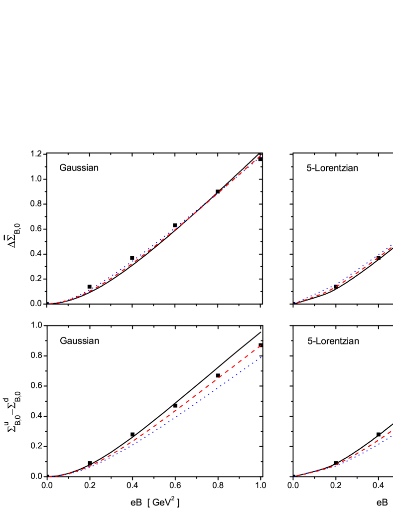
Figure 1: Normalized condensates as functions of the magnetic field at $T=0$. Upper panel: subtracted flavor average; lower panel: flavor difference [see Eq. (43) and the text below]. Solid (black), dashed (red), and dotted (blue) curves correspond to parameterizations leading to $(-\langle\bar{q}q\rangle^{\rm reg}_{0,0})^{1/3}=220$, 230, and 240 MeV, respectively. Full square symbols indicate LQCD results taken from Ref. Bali:2012zg .

We turn now to our numerical results for a system at finite temperature. In the upper panels of Fig. 2 we show the behavior of the averaged chiral condensate $\bar{\Sigma}_{B,T}$ and the traced Polyakov loop $\Phi$ as functions of the temperature, for three representative values of the external magnetic field $B$, namely $B=0$, 0.6, and 1 GeV². The curves correspond to parameter sets leading to $(-\langle\bar{q}q\rangle^{\rm reg}_{0,0})^{1/3}=230$ MeV and a polynomial Polyakov-loop potential with $T_{0}=210$ MeV. Given a value of $B$, it is seen from the figure that for the cases of both Gaussian and 5-Lorentzian form factors the chiral restoration and deconfinement transitions proceed as smooth crossovers, at approximately the same critical temperatures. For definiteness, we take these temperatures from the maxima of the chiral and PL susceptibilities, which we define as the derivatives $\chi_{\rm ch}=-\partial[(\langle\bar{u}u\rangle^{\rm reg}_{B,T}+\langle\bar{d}d\rangle^{\rm reg}_{B,T})/2]/\partial T$ and $\chi_{\Phi}=\partial\Phi/\partial T$, respectively. Our results for the behavior of the susceptibilities as functions of the temperature, for $B=0$, 0.6, and 1 GeV², are shown in the lower panels of Fig. 2.

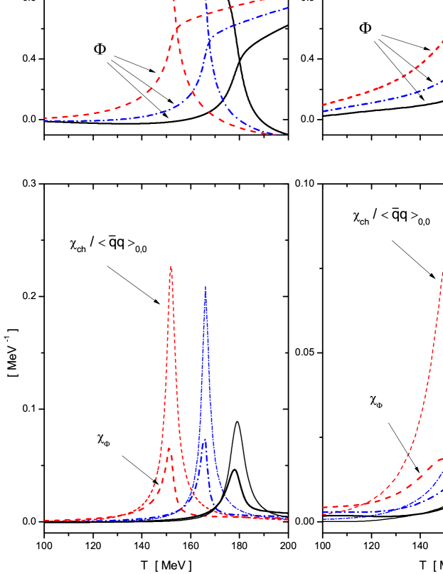
Figure 2: Upper panels: normalized flavor average condensate and traced Polyakov loop as functions of the temperature, for three representative values of $eB$. Lower panels: behavior of the corresponding chiral and PL susceptibilities as functions of the temperature.

Table 2: Critical temperatures for $B=0$ and various parametrizations.

	Gaussian			5-Lorentzian
$(-\langle\,q\bar{q}\,\rangle_{0,0}^{\rm reg})^{1/3}$ (MeV)	220	230	240	220	230	240
Chiral $T_{c}$ (MeV)	182.1	179.1	177.4	177.0	177.0	177.8
Deconfinement $T_{c}$ (MeV)	182.1	178.0	175.8	174.8	174.7	175.5

The chiral restoration and deconfinement critical temperatures obtained in the absence of external magnetic field for different parametrizations are quoted in Table 2. It is seen that in all cases the splitting between both critical temperatures is below 5 MeV, which is consistent with the results obtained in lattice QCD. From Table 2 it is also seen that the values of critical temperatures do not vary significantly with the parametrization (recalling that in all cases the parameters have been fixed to reproduce the empirical values of the pion mass and decay constant). On the other hand, the critical temperatures in Table 2 are found to be somewhat higher than those obtained from LQCD, which lie around 160 MeV Aoki:2009sc ; Bazavov:2011nk . In fact, the value of $T_{c}$ and the steepness of the transition depend on the form of the Polyakov-loop potential. It is found that the logarithmic PL potential Roessner:2006xn leads in general to steep transitions (which can be even of first order for certain values of the parameters), whereas the “improved” PL potentials [see Eqs. (36) and (37)] lead to a smoother behavior that shows a better agreement with LQCD results Carlomagno:2013ona . In particular, for an “improved polynomial” PL potential, one can get $T_{c}\simeq 160$ to 165 MeV, depending on the parametrization. It is worth noticing that in the absence of the interaction with the Polyakov loop the values of $T_{c}$ drop down to about 130 MeV Pagura:2016pwr .

Let us discuss the effect of the magnetic field on the phase transition features. From Fig. 2 it is seen that the splitting between the chiral restoration and deconfinement critical temperatures remains very small in the presence of the external field (in fact, a detailed analysis shows that the splitting gets reduced for larger values of $eB$). In addition, it is seen that the nonlocal NJL models show inverse magnetic catalysis. Indeed, contrary to what happens e.g. in the standard local NJL model Kharzeev:2012ph ; Andersen:2014xxa ; Miransky:2015ava , in our models the chiral restoration critical temperature becomes lower as the external magnetic field is increased. This is related to the fact that the condensates do not show in general a monotonic increase with $B$ for a fixed value of the temperature. The situation is illustrated in Fig. 3, where we show the behavior of the averaged difference $\Delta\bar{\Sigma}_{B,T}$ as a function of $eB$, for $T=0$ and for values of the temperature in the critical region. The curves correspond to models with Gaussian (left) and Lorentzian (right) form factors, $(-\langle\bar{q}q\rangle^{\rm reg}_{0,0})^{1/3}=230$ MeV, polynomial PL potential. For these parametrizations, the critical temperatures for $B=0$ are slightly below 180 MeV (see Table 2). While for $T=0$ the value of $\Delta\bar{\Sigma}_{B,0}$ shows a monotonic growth with the external magnetic field, it is seen that when the temperatures get closer to the critical values the curves have a maximum and then start to decrease for increasing $B$. This is the typical behavior associated to IMC and observed from lattice QCD results, see e.g. Fig. 2 of Ref. Bali:2012zg . Qualitatively similar results are found for the other parametrizations in Table I. Finally, in Fig. 4 we plot our results for the chiral restoration critical temperatures $T_{c}(B)$, normalized to the corresponding values at vanishing external magnetic field. The figure includes the curves for nonlocal NJL models with Gaussian (left) and 5-Lorentzian (right) form factors and different parameter sets (see the caption). The gray bands in both panels show the results obtained in LQCD, taken from Ref. Bali:2012zg . For comparison, for the Gaussian form factor we have plotted with thin lines the results for the “improved polynomial”. Thick lines for both Gaussian and 5-Lorentzian form factors correspond to the polynomial PL potential in Eq. (33). Results for the logarithmic PL potential have been omitted, since (as stated above) the transitions are found to be too steep in comparison with LQCD results. From the figure it is clearly seen that the inverse magnetic catalysis effect is observed for all considered parametrizations. In addition, for a given form factor, the effect is found to be stronger for parameter sets leading to a lower absolute value of the chiral quark condensates. As a general conclusion, it can be stated that the behavior of the critical temperatures with the external magnetic field is compatible with LQCD results, for phenomenologically adequate values of the chiral condensate.

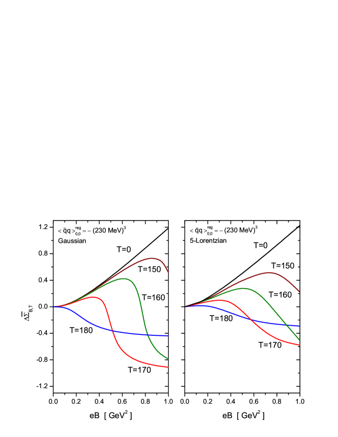
Figure 3: Subtracted normalized flavor average condensate as a function of $eB$ for different representative temperatures. Left and right panels correspond to Gaussian and 5-Lorentzian form factors, respectively, with $(-\langle\bar{q}q\rangle^{\rm reg}_{0,0})^{1/3}=230$ MeV and polynomial PL potential. Temperature values are given in MeV.

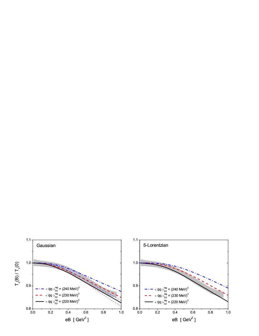
Figure 4: Normalized critical temperatures as functions of $eB$ for various model parametrizations. For comparison, LQCD results of Ref. Bali:2012zg are indicated by the gray band. Left and right panels correspond to Gaussian and 5-Lorentzian form factors, respectively.

To shed some light on the mechanism that leads to the IMC effect in our model it is worth noticing that the nonlocal form factor turns out to be a function of the external magnetic field. This can be clearly seen from Eq. (17). In addition, it is important to take into account that in nonlocal NJL-like models the form factors play the role of some finite-range gluon-mediated effective interaction. Thus, the magnetic field dependence of the form factor can be understood as originated by the backreaction of the sea quarks on the gluon fields. It is interesting to consider the effective mass for the particular case of a Gaussian form factor, given by Eq. (46). It can be seen that in this case the components of the momentum that are parallel and transverse to the magnetic field become disentangled. While for the $3,4$ components the original exponential form $\exp{(-\bar{p}^{2}/\Lambda^{2})}$ is maintained, the $1,2$ (transverse) part leads to a factor given by a ratio of polynomials in $|q_{f}B|/\Lambda^{2}$, which goes to zero for large $B$. In this way, for any value of $k$, the strength of the effective coupling decreases as $B$ increases. This is analogous to what happens with the $B$-dependent coupling constants considered e.g. in Refs. Ferreira:2014kpa ; Farias:2014eca , and thus the IMC effect can be understood on these grounds.

IV Summary & conclusions

We have studied the behavior of strongly interacting matter under a uniform static external magnetic field in the context of a nonlocal chiral quark model. In this approach, which can be viewed as an extension of the Polyakov$-$Nambu$-$Jona-Lasinio model, the effective couplings between quark-antiquark currents include nonlocal form factors that regularize ultraviolet divergences in quark loop integrals and lead to a momentum-dependent effective mass in quark propagators. We have worked out the formalism introducing Ritus transforms of Dirac fields, which allow us to obtain closed analytical expressions for the gap equations, the chiral quark condensate, and the quark propagator. In addition, we have shown that these expressions can also be obtained in the framework of a Schwinger-Dyson approach.

We have considered the case of Gaussian and Lorentzian form factors, choosing some sets of model parameters that allow us to reproduce the empirical values of the pion mass and decay constants. At zero temperature, with these parameterizations we have calculated the behavior of the subtracted flavor average condensate $\Delta\bar{\Sigma}_{B,0}$ and the normalized condensate difference $\Sigma^{u}_{B,0}-\Sigma^{d}_{B,0}$ as functions of the external magnetic field $B$. Our results show the expected effect of magnetic catalysis (condensates behave as growing functions of $B$), the curves being in quantitative agreement with lattice QCD calculations with slight dependence on the parametrization.

Finally we have extended the calculations to finite temperature systems, including the couplings of fermions to the Polyakov loop. We have defined chiral and PL susceptibilities in order to study the chiral restoration and deconfinement transitions, which turn out to proceed as smooth crossovers for the polynomial PL potential considered. From our numerical calculations, on one hand it is seen that, for all considered values of $B$, both transitions take place at approximately the same temperature, in agreement with LQCD predictions. On the other hand, it is found that for temperatures close to the transition region the subtracted flavor average condensate $\Delta\bar{\Sigma}_{B,T}$ becomes a nonmonotonic function of $B$, which eventually leads to the phenomenon of inverse magnetic catalysis, i.e., a decrease of the critical temperature when the magnetic field gets increased. This feature is also in qualitative agreement with LQCD expectations. Moreover, for some parameterizations we find a remarkably good quantitative agreement with the results from LQCD calculations for the behavior of the normalized critical temperatures with $B$ (see Fig. 4). The values of the critical temperature at $T=0$, which show some dependence on the parameterization and the PL potential, lie also within the range estimated by LQCD results.

It is interesting to compare the nonlocal models with approaches in which IMC is obtained by considering some ad hoc dependence of the effective couplings on $B$ and/or $T$. The naturalness of the IMC behavior in our framework can be understood by noticing that for a given Landau level the associated nonlocal form factor turns out to be a function of the external magnetic field, according to the convolution in Eq. (17). Since the form factors can be identified with some gluon-mediated effective interaction, the dependence on the magnetic field can be seen as originated by the backreaction of the quarks on the gluon fields.

Appendix A: Ritus eigenfunctions and Ritus transforms

In this Appendix we provide the explicit form of the Ritus eigenfunctions Ritus:1978cj and discuss some of the their properties. These functions satisfy the eigenvalue equation

$$\Pi^{2}\ \mathbb{E}_{\bar{p}}(x)\ =\ \epsilon_{\bar{p}}\ \mathbb{E}_{\bar{p}}(x)\ ,$$ (A1)

where, in accordance with the definition in the main text, $\Pi=-i\hbox to0.0pt{/\hss}\partial-qBx_{1}\gamma_{2}$. Here, $\bar{p}=(k,p_{2},p_{3},p_{4})$ represents the set of quantum numbers needed to label the eigenstates, the eigenvalues of which are given by $\epsilon_{\bar{p}}=-(2k|qB|+p_{3}^{2}+p_{4}^{2})$. Working in Euclidean space and choosing the Weyl representation for the Dirac matrices,

$$\vec{\gamma}=\begin{pmatrix}0&\vec{\sigma}\\ -\vec{\sigma}&0\end{pmatrix}\ ,\qquad\gamma_{4}=i\gamma_{0}=i\begin{pmatrix}0&\mathcal{I}\\ \mathcal{I}&0\end{pmatrix}\ ,$$ (A2)

one has

$$\mathbb{E}_{\bar{p}}(x)\ =\ \sum_{\lambda=\pm}E_{\bar{p}\lambda}(x)\,\Delta^{\lambda}\ ,$$ (A3)

where $\Delta^{+}=\mbox{diag}(1,0,1,0)$, $\Delta^{-}=\mbox{diag}(0,1,0,1)$, and

$$E_{\bar{p}\lambda}(x)\ =\ N_{k_{\lambda}}\ e^{i(p_{2}x_{2}+p_{3}x_{3}+p_{4}x_{4})}\,D_{k_{\lambda}}(\rho)\ ,$$ (A4)

where $\rho=s\sqrt{2/|qB|}\,(qB\,x_{1}-p_{2})$, with $s=\mbox{sign}(qB)$. The integer index $k_{\lambda}$ is related to the quantum number $k$ by

$$k_{\pm}=k-\frac{1}{2}\pm\frac{s}{2}\ ,$$ (A5)

while $N_{n}=(4\pi|qB|)^{1/4}/\sqrt{n!}\,$. In Eq. (A4) we have introduced the cylindrical parabolic functions defined by

$$D_{n}(x)\ =\ 2^{-n/2}\,e^{-x^{2}/4}\,H_{n}(x/\sqrt{2})\ ,$$ (A6)

where $H_{n}(x)$ are the Hermite polynomials, with the standard convention $H_{-1}(x)=0$. In fact, strictly speaking, for $k=0$ the Ritus eigenfunction $\mathbb{E}_{\bar{p}}(x)$ should be defined as a $2\times 2$ matrix

$$\mathbb{E}_{(0,p_{2},p_{3},p_{4})}(x)\ =\ (4\pi|qB|)^{1/4}\ e^{i(p_{2}x_{2}+p_{3}x_{3}+p_{4}x_{4})}\,e^{-\rho^{2}/4}\;\leavevmode\hbox{\small 1\kern-3.8pt\normalsize 1}_{(2\times 2)}\ ,$$ (A7)

where $\leavevmode\hbox{\small 1\kern-3.8pt\normalsize 1}_{(2\times 2)}$ is the identity matrix in the subspace where $E_{\bar{p}\lambda}(x)$ is nonzero. On the other hand, it is easily seen that the matrices $\Delta^{\lambda}$ satisfy

$$\Delta^{\pm}\Delta^{\pm}=\Delta^{\pm}\ ,\quad\Delta^{\pm}\Delta^{\mp}=0\ ,\quad\Delta^{\pm}\gamma_{\perp}=\gamma_{\perp}\,\Delta^{\mp}\ ,\quad\Delta^{\pm}\gamma_{\parallel}=\gamma_{\parallel}\,\Delta^{\pm}\ ,$$ (A8)

where $\gamma_{\perp}=(\gamma_{1},\gamma_{2})$ and $\gamma_{\parallel}=(\gamma_{3},\gamma_{4})$.

As expected, along the direction of the magnetic field the function $\mathbb{E}_{\bar{p}}(x)$ preserves the form of the energy eigenfunction of a free particle, being labeled by a continuous index $p_{3}$ that corresponds to the momentum component parallel to $\vec{B}$. This is also the situation in the direction of the imaginary time. On the other hand, the quantum numbers corresponding to the plane $x_{1}\,x_{2}$ depend on the gauge used to describe the vector potential $A_{\mu}$. We have chosen the Landau gauge, for which the states associated with the $x_{1}$ direction are quantized and labeled by the integer index $k$. Along the $x_{2}$ direction, the eigenfunction has the form of that of a free particle, with the particularity that the eigenvalues do not depend on $p_{2}$, and hence the states are degenerated. This last property leads to the useful relation

$$\int\frac{dp_{2}}{2\pi}\;\mathbb{E}_{\bar{p}}(x)\,\mathbb{\bar{E}}_{\bar{p}}(x)\ =\ \int\frac{dp_{2}}{2\pi}\;\mathbb{\bar{E}}_{\bar{p}}(x)\,\mathbb{E}_{\bar{p}}(x)\ =\ |qB|\,P_{k,s}\ ,$$ (A9)

where we have defined $\mathbb{\bar{E}}_{\bar{p}}=\gamma_{0}\,\mathbb{E}_{\bar{p}}^{\dagger}\,\gamma_{0}$ and $P_{k,\pm 1}=(1-\delta_{k0})\,\mathcal{I}+\delta_{k0}\,\Delta^{\pm}$. The operators $P_{k,\pm 1}$ are projectors; i.e., they satisfy $P_{k,s}=(P_{k,s})^{2}$. It is also seen that $P_{k,s}\;\mathbb{E}_{\bar{p}}=\mathbb{E}_{\bar{p}}\;P_{k,s}=\mathbb{E}_{\bar{p}}\,$.

The Ritus functions $\mathbb{E}_{\bar{p}}(x)$ satisfy orthonormality and completeness relations, namely

$$\int d^{4}x\;\mathbb{\bar{E}}_{\bar{p}}(x)\,\mathbb{E}_{\bar{p}\,^{\prime}}(x)\ =\ \hat{\delta}_{\bar{p},\bar{p}\,^{\prime}}\,P_{k,s}\ ,$$ (A10)

$$\int\!\!\!\!\!\!\!\sum_{\bar{p}}\;\mathbb{E}_{\bar{p}}(x)\,\mathbb{\bar{E}}_{\bar{p}}(x^{\prime})\ =\ \delta^{(4)}(x-x^{\prime})\ ,$$ (A11)

where the following shorthand notations have been introduced

$$\int\!\!\!\!\!\!\!\sum_{\bar{p}}\equiv\frac{1}{2\pi}\sum_{k=0}^{\infty}\int\frac{dp_{2}}{2\pi}\,\frac{dp_{3}}{2\pi}\,\frac{dp_{4}}{2\pi}\,\ ,\quad\hat{\delta}_{\bar{p},\bar{p}\,^{\prime}}\equiv(2\pi)^{4}\,\delta_{kk^{\prime}}\,\delta(p_{2}-p^{\prime}_{2})\,\delta(p_{3}-p^{\prime}_{3})\,\delta(p_{4}-p^{\prime}_{4})\ .$$ (A12)

In addition, they satisfy the important identity

$$\Pi\;\mathbb{E}_{\bar{p}}(x)\ =\ \mathbb{E}_{\bar{p}}(x)\,\Big{(}\!-\!s\,\sqrt{2k|qB|}\ \gamma_{2}+p_{\parallel}\cdot\gamma_{\parallel}\Big{)}\ ,$$ (A13)

where $p_{\parallel}=(p_{3},p_{4})$.

Given the Ritus functions, one can define the Ritus transform of some arbitrary Dirac function $\psi(x)$. One has

$$\psi_{\bar{p}}=\int d^{4}x\ \mathbb{\bar{E}}_{\bar{p}}(x)\ \psi(x)\ ,\qquad\bar{\psi}_{\bar{p}}=\int d^{4}x\ \bar{\psi}(x)\ \mathbb{E}_{\bar{p}}(x)\ ,$$ (A14)

together with the inverse transforms

$$\psi(x)=\int\!\!\!\!\!\!\!\sum_{\bar{p}}\;\mathbb{E}_{\bar{p}}(x)\ \psi_{\bar{p}}\ ,\qquad\bar{\psi}(x)=\int\!\!\!\!\!\!\!\sum_{\bar{p}}\;\bar{\psi}_{\bar{p}}\ \mathbb{\bar{E}}_{\bar{p}}(x)\ .$$ (A15)

In the same way, the Ritus transform $\mathcal{O}_{\bar{p},\bar{p}\,^{\prime}}$ of an arbitrary operator $\mathcal{O}_{x,x^{\prime}}$ satisfies

$$\mathcal{O}_{\bar{p},\bar{p}\,^{\prime}} = \int d^{4}x\ d^{4}x^{\prime}\ \ \mathbb{\bar{E}}_{\bar{p}}(x)\ \mathcal{O}_{x,x^{\prime}}\ \mathbb{E}_{\bar{p}\,^{\prime}}(x^{\prime})\ ,$$ (A16)

$$\mathcal{O}_{x,x^{\prime}} = \int\!\!\!\!\!\!\!\sum_{\;\,\bar{p},\bar{p}\,^{\prime}}\ \mathbb{E}_{\bar{p}}(x)\ \mathcal{O}_{\bar{p},\bar{p}\,^{\prime}}\ \mathbb{\bar{E}}_{\bar{p}\,^{\prime}}(x^{\prime})\ .$$ (A17)

Appendix B: Details of the evaluation of $G^{\lambda,f}_{\bar{p},\bar{p}\,^{\prime}}$

We start from the relation in Eq. (16),

$$G^{\lambda,f}_{\bar{p},\bar{p}\,^{\prime}}=\int d^{4}x\ d^{4}x^{\prime}\ E^{*}_{\bar{p}\lambda}(x)\ \mathcal{G}(x-x^{\prime})\,\exp\left[i\Phi_{f}(x,x^{\prime})\right]\,E_{\bar{p}\,^{\prime}\lambda}(x^{\prime})\ ,$$ (B1)

where $\Phi_{f}(x,x^{\prime})=(q_{f}B/2)\,(x_{2}-x_{2}^{\prime})\,(x_{1}+x_{1}^{\prime})$, and the functions $E_{\bar{p}\lambda}(x)$ are given in Eq. (A4). To work out this expression, we introduce the Fourier transform of $\mathcal{G}(x)$,

$$g(t^{2})=\int d^{4}x\ e^{-it\,\cdot x}\;\mathcal{G}(x)\ ,$$ (B2)

and perform the change of variables $x=z+y/2$, $x^{\prime}=z-y/2$. In this way, we get

$$G^{\lambda,f}_{\bar{p},\bar{p}\,^{\prime}}=\int\frac{d^{4}t}{(2\pi)^{4}}\ g(t^{2})\int d^{4}y\ d^{4}z\ E^{*}_{p\lambda}(z+y/2)\ \exp(it\cdot y)\,\exp(iq_{f}By_{2}z_{1})\;E_{p^{\prime}\lambda}(z-y/2)\ .$$ (B3)

Given the explicit form of the functions $E_{\bar{p}\lambda}(x)$, the integrals over $z_{2},z_{3},z_{4}$ and $y_{3},y_{4}$ can be easily performed. We obtain

$$G^{\lambda,f}_{\bar{p},\bar{p}\,^{\prime}} = (2\pi)^{3}\,\delta(p_{2}-p_{2}^{\prime})\,\delta(p_{3}-p^{\prime}_{3})\,\delta(p_{4}-p^{\prime}_{4})\;\Gamma^{\lambda,f}_{k,k^{\prime},p_{\parallel}}\ ,$$ (B4)

where

$$\Gamma^{\lambda,f}_{k,k^{\prime},p_{\parallel}} = \ N_{k_{\lambda}}N_{k^{\prime}_{\lambda}}\int\frac{d^{2}t_{\perp}}{(2\pi)^{2}}\ g(t_{\perp}^{2}+p_{\parallel}^{2})\int dz_{1}d^{2}y_{\perp}$$ (B5)

$$\exp(-ip_{2}y_{2})\,\exp(it_{\perp}\cdot y_{\perp})\,\exp(iq_{f}By_{2}z_{1})\;D_{k_{\lambda}}(\rho)\;D_{k^{\prime}_{\lambda}}(\rho^{\prime})\ ,$$

with $t_{\perp}=(t_{1},t_{2})$ and

$$\rho=s_{f}\sqrt{\frac{2}{|q_{f}B|}}\;\big{[}q_{f}B\ (z_{1}+y_{1}/2)-p_{2}\big{]}\ ,\quad\rho^{\prime}=s_{f}\sqrt{\frac{2}{|q_{f}B|}}\;\big{[}q_{f}B\ (z_{1}-y_{1}/2)-p_{2}\big{]}\ .$$ (B6)

We recall here that $s_{f}=\mbox{sign}(q_{f}B)$, while $k_{\lambda}$ is related to $k$ by Eq. (A5). We note now that the integration over $y_{2}$ introduces a factor $2\pi\,\delta(q_{f}Bz_{1}-p_{2}+t_{2})$, which allows us to easily perform the integral over $t_{2}$. Taking into account the explicit form of $\rho$ and $\rho^{\prime}$, we get

$$\Gamma^{\lambda,f}_{k,k^{\prime},p_{\parallel}} = \frac{1}{\left[2\pi\;2^{{k_{\lambda}}+{k^{\prime}_{\lambda}}}\,{k_{\lambda}}!\,{k^{\prime}_{\lambda}}!\right]^{1/2}}\int d\gamma\ d\eta\ d\psi\ \ g\Big{[}\frac{|q_{f}B|}{2}(\gamma^{2}+\eta^{2})\,+\,p_{\parallel}^{2}\Big{]}\ \times$$ (B7)

$$\exp(i\gamma\psi)\,\exp\Big{(}\!-\frac{\eta^{2}+\psi^{2}}{2}\Big{)}\;H_{k_{\lambda}}\Big{(}\frac{\eta+\psi}{\sqrt{2}}\Big{)}\;H_{k^{\prime}_{\lambda}}\Big{(}\frac{\eta-\psi}{\sqrt{2}}\Big{)}\ ,$$

where we have used the expression of $D_{n}$ in terms of Hermite polynomials, Eq. (A6), and for convenience we have introduced the dimensionless variables

$$\gamma=\sqrt{\frac{2}{|q_{f}B|}}\ t_{1}\ ,\qquad\eta=s_{f}\sqrt{\frac{2}{|q_{f}B|}}\left(q_{f}Bz_{1}+p_{2}\right)\ ,\qquad\psi=\sqrt{\frac{|q_{f}B|}{2}}\ y_{1}\ .$$ (B8)

Making a new change of variables to polar coordinates $r,\phi$ in the $\gamma\eta$ plane, we get

$$\Gamma^{\lambda,f}_{k,k^{\prime},p_{\parallel}} = \int_{0}^{\infty}dr\ r\ \ g\Big{(}\frac{|q_{f}B|}{2}\,r^{2}\,+\,p_{\parallel}^{2}\Big{)}\,\exp(-r^{2}/2)\;I^{\lambda}_{k,k^{\prime}}(r)\ ,$$ (B9)

where

$$I^{\lambda}_{k,k^{\prime}}(r) = \frac{1}{\left[2\pi\;2^{{k_{\lambda}}+{k^{\prime}_{\lambda}}}\,{k_{\lambda}}!\,{k^{\prime}_{\lambda}}!\right]^{1/2}}\int_{0}^{2\pi}d\phi\int_{-\infty}^{\infty}d\psi\ \exp\Big{[}-(\psi-ir\cos\phi)^{2}/2\,\Big{]}\ \times$$ (B10)

$$\qquad\qquad\qquad\qquad\qquad H_{k_{\lambda}}\Big{(}\frac{r\sin\phi+\psi}{\sqrt{2}}\Big{)}\;H_{k^{\prime}_{\lambda}}\Big{(}\frac{r\sin\phi-\psi}{\sqrt{2}}\Big{)}\ .$$

Next we carry out a translation into the complex plane $\psi$, namely $\psi\rightarrow\psi^{\prime}=\psi-ir\cos\phi$. Since the integrand in Eq. (B10) is an analytic function, making use of Cauchy’s theorem one can show that the integration path can be taken along the ${\rm Im}\,\psi\,^{\prime}=0$ axis. Thus, we obtain

$$I^{\lambda}_{k,k^{\prime}}(r) = \frac{1}{\left[2\pi\;2^{{k_{\lambda}}+{k^{\prime}_{\lambda}}}\,{k_{\lambda}}!\,{k^{\prime}_{\lambda}}!\right]^{1/2}}\int_{0}^{2\pi}d\phi\int_{-\infty}^{\infty}d\psi\;\exp(-\psi^{2}/2)$$ (B11)

$$\qquad\qquad\qquad\qquad\quad H_{k_{\lambda}}\Big{[}\frac{ir\exp{(-i\phi)}+\psi}{\sqrt{2}}\Big{]}\;H_{k^{\prime}_{\lambda}}\Big{[}\frac{-ir\exp{(i\phi)}-\psi}{\sqrt{2}}\Big{]}\ .$$

Next, we use the relation $H_{n}(-x)=(-1)^{n}H_{n}(x)$ and the identity (see Eq. (7.377) of Ref. grad )

$$\int_{-\infty}^{\infty}dx\;e^{-x^{2}}H_{m}(x+y)\ H_{n}(x+z)\ =\ 2^{n}\;\sqrt{\pi}\;m!\;z^{n-m}\;L^{n-m}_{m}(-2yz)\ ,\quad n\geq m\ ,$$ (B12)

where $L^{a}_{b}(x)$ are generalized Laguerre polynomials. Finally, using

$$\int_{0}^{2\pi}d\phi\ \exp(i\phi\,m)\ =\ 2\pi\,\delta_{m0}\ ,$$ (B13)

we obtain

$$I^{\lambda}_{k,k^{\prime}}(r)\ =\ 2\pi\,(-1)^{k_{\lambda}}\,L_{k_{\lambda}}(r^{2})\;\delta_{kk^{\prime}}\ .$$ (B14)

Replacing Eq. (B14) in Eq. (B9), and taking into account Eq. (B4), after a new change of variables $r\to|p_{\perp}|=r\sqrt{|q_{f}B|/2}$ we end up with

$$G^{\lambda,f}_{\bar{p},\bar{p}^{\prime}}\ =\ \hat{\delta}_{\bar{p},\bar{p}\,^{\prime}}\ g^{\lambda,f}_{k,p_{\parallel}}\ ,$$ (B15)

where $g^{\lambda,f}_{k,p_{\parallel}}$ is given in Eq. (17).

Appendix C: Mean field quark propagator

In this Appendix, we outline the derivation of the $u$ and $d$ quark propagators within the MFA. We start from the two-point function in Ritus space $\mathcal{D}^{\mbox{\tiny MFA},f}_{\bar{p},\bar{p}\,^{\prime}}$ which, as discussed in the main text, is diagonal in Landau/momentum indices $\bar{p}$. The mean field quark propagators in this space, for quark flavors $f=u,d$, are then given by

$$S^{\mbox{\tiny MFA},f}_{\bar{p},\bar{p}\,^{\prime}}\ =\ \big{(}\mathcal{D}^{\mbox{\tiny MFA},f}_{\bar{p},\bar{p}\,^{\prime}}\big{)}^{-1}\ =\ \hat{\delta}_{\bar{p},\bar{p}\,^{\prime}}\,\big{(}{\mathcal{D}}^{f}_{k,p_{\parallel}}\big{)}^{-1}\ ,$$ (C1)

with ${\mathcal{D}}^{f}_{k,p_{\parallel}}$ given by Eq. (19). Since this operator is nondiagonal only in Dirac space, it can be easily inverted. Defining ${\cal S}^{f}_{k,p_{\parallel}}=({\mathcal{D}}^{f}_{k,p_{\parallel}})^{-1}$, one finds that ${\cal S}^{f}_{k,p_{\parallel}}$ can be written as

$${\cal S}^{f}_{k,p_{\parallel}}\ =\ \sum_{\lambda=\pm}\Big{[}\hat{A}^{\lambda,f}_{k,p_{\parallel}}-\hat{B}^{\lambda,f}_{k,p_{\parallel}}\,p_{\parallel}\cdot\gamma_{\parallel}+s_{f}\sqrt{2kB_{f}}\big{(}\hat{C}^{\lambda,f}_{k,p_{\parallel}}-\hat{D}^{\lambda,f}_{k,p_{\parallel}}\,p_{\parallel}\cdot\gamma_{\parallel}\big{)}\gamma_{2}\Big{]}\Delta^{\lambda}\ ,$$ (C2)

where we have defined $B_{f}=|q_{f}B|$, and the functions $\hat{A}^{\lambda,f}_{k,p_{\parallel}}$ to $\hat{D}^{\lambda,f}_{k,p_{\parallel}}$ are given in Eqs. (28-31). Notice that in the particular case $k=0$ (i.e. $k_{\lambda}=0$ or $-1$) the Dirac space is reduced to a two-dimensional one; therefore, only the coefficients $\hat{A}^{\lambda,f}_{k,p_{\parallel}}$ and $\hat{B}^{\lambda,f}_{k,p_{\parallel}}$ with $k_{\lambda}=0$ need to be considered.

To find the expression for the propagator in coordinate space, we have to perform the Ritus antitransform of $S^{\mbox{\tiny MFA},f}_{\bar{p},\bar{p}\,^{\prime}}$. One has

$$\!\!\!\!\!\!\!\!\!\!\!\!\!S^{\mbox{\tiny MFA},f}_{x,x^{\prime}} = \int\!\!\!\!\!\!\!\sum_{\;\;\bar{p},\bar{p}\,^{\prime}}\;\mathbb{E}_{\bar{p}}(x)\,S^{\mbox{\tiny MFA},f}_{\bar{p},\bar{p}\,^{\prime}}\;\bar{\mathbb{E}}_{\bar{p}\,^{\prime}}(x^{\prime})$$ (C3)

$$= \frac{1}{2\pi}\sum_{k=0}^{\infty}\int\frac{d^{2}p_{\parallel}}{(2\pi)^{2}}\,e^{ip_{\parallel}\cdot\Delta x_{\parallel}}\sum_{\lambda,\lambda^{\prime}=\pm}I^{\lambda\lambda^{\prime}}\,\Big{[}\delta_{\lambda\lambda^{\prime}}\big{(}\hat{A}^{\lambda,f}_{k,p_{\parallel}}-\hat{B}^{\lambda,f}_{k,p_{\parallel}}\,p_{\parallel}\cdot\gamma_{\parallel}\big{)}\Delta^{\lambda}\,$$

$$\qquad\qquad+s_{f}\sqrt{2kB_{f}}\,(1-\delta_{\lambda\lambda^{\prime}})\big{(}\hat{C}^{\lambda^{\prime},f}_{k,p_{\parallel}}-\hat{D}^{\lambda^{\prime},f}_{k,p_{\parallel}}\,p_{\parallel}\cdot\gamma_{\parallel}\big{)}\gamma_{2}\,\Delta^{\lambda^{\prime}}\Big{]}\ ,$$

where we have defined $\Delta x_{\parallel}=(\Delta x_{3},\Delta x_{4})$, with $\Delta x_{i}=x_{i}-x^{\prime}_{i}$, and the integrals $I^{\lambda\lambda^{\prime}}$ are given by

$$I^{\lambda\lambda^{\prime}}\ =\ N_{k_{\lambda}}\,N_{k_{\lambda^{\prime}}}\int\frac{dp_{2}}{2\pi}\;e^{ip_{2}(x_{2}-x_{2}^{\prime})}\,D_{k_{\lambda}}(\rho)\,D_{k_{\lambda^{\prime}}}(\rho^{\prime})\ ,$$ (C4)

with $\rho^{(\prime)}=s_{f}\sqrt{2/B_{f}}[\,q_{f}B\,x_{1}^{(\prime)}-p_{2}]=\sqrt{2B_{f}}[\,x_{1}^{(\prime)}-(s_{f}/B_{f})\,p_{2}]$. Let us analyze separately the integrals $I^{\pm\pm}$ and $I^{\pm\mp}$. Considering the explicit expressions for $N_{k_{\lambda}}$ and $D_{k_{\lambda}}(x)$ [see Eq. (A6)], and performing the translation $p_{2}=q_{2}+s_{f}B_{f}(x_{1}+x_{1}^{\prime})/2$, one has

$$I^{\lambda\lambda} = \sqrt{\frac{B_{f}}{\pi}}\,\frac{2^{-k_{\lambda}}}{k!}\;\exp[i\Phi_{f}(x,x^{\prime})]\,\exp(-B_{f}\Delta x_{1}^{2}/4)\int_{-\infty}^{\infty}dq_{2}\;\exp(iq_{2}\Delta x_{2})\,\times$$ (C5)

$$\exp(-q_{2}^{2}/B_{f})\;H_{k_{\lambda}}\Big{(}\frac{\sqrt{B_{f}}\Delta x_{1}}{2}-\frac{s_{f}q_{2}}{\sqrt{B_{f}}}\Big{)}\;H_{k_{\lambda}}\Big{(}-\frac{\sqrt{B_{f}}\Delta x_{1}}{2}-\frac{s_{f}q_{2}}{\sqrt{B_{f}}}\Big{)}\ ,$$

where $\Phi_{f}(x,x^{\prime})$ is the already defined Schwinger phase. Now it is possible to carry out a translation in the complex plane to a new variable $\omega=(q_{2}-iB_{f}\Delta x_{2}/2)s_{f}/\sqrt{B_{f}}$. Since the integrand is an analytic function in the whole plane, the integral can be calculated along the ${\rm Im}\,\omega=0$ axis. One gets in this way

$$I^{\lambda\lambda} = \frac{B_{f}}{\sqrt{\pi}}\,\frac{2^{-k_{\lambda}}}{k!}\;\exp[i\Phi_{f}(x,x^{\prime})]\,\exp(-B_{f}\Delta x_{\perp}^{2}/4)\int_{-\infty}^{\infty}d\omega\;\exp(-\omega^{2})\,\times$$ (C6)

$$H_{k_{\lambda}}\Big{[}\omega-\sqrt{B_{f}}(\Delta x_{1}-is_{f}\Delta x_{2})/2\Big{]}\;H_{k_{\lambda}}\Big{[}\omega+\sqrt{B_{f}}(\Delta x_{1}+is_{f}\Delta x_{2})/2\Big{]}\ ,$$

where $\Delta x_{\perp}=(\Delta x_{1},\Delta x_{2})$. The integral in Eq. (C6) can be evaluated using the relation in Eq. (B12), which leads to

$$I^{\lambda\lambda}\ =\ B_{f}\,\exp[i\Phi_{f}(x,x^{\prime})]\,\exp[-B_{f}\Delta x_{\perp}^{2}/4]\;L_{k_{\lambda}}\big{(}B_{f}\Delta x_{\perp}^{2}/2\big{)}\ .$$ (C7)

Next, let us consider the integral

$$K^{(0)}(m,y_{\perp})\ =\ \int d^{2}p_{\perp}\;e^{ip_{\perp}\cdot y_{\perp}}\;\exp(-p_{\perp}^{2}/B_{f})\;L_{m}(2p_{\perp}^{2}/B_{f})\ ,$$ (C8)

where $p_{\perp}=(p_{1},p_{2})$, $y_{\perp}=(y_{1},y_{2})$. One has

$$K^{(0)}(m,y_{\perp}) = \int_{0}^{\infty}d\left|p_{\perp}\right|\;\left|p_{\perp}\right|\,\exp(-p_{\perp}^{2}/B_{f})\,L_{m}(2p_{\perp}^{2}/B_{f})\;\int_{0}^{2\pi}d\theta\;e^{i\left|p_{\perp}\right|(y_{1}\cos\theta+y_{2}\sin\theta)}$$ (C9)

$$= 2\pi\int_{0}^{\infty}d\left|p_{\perp}\right|\;\left|p_{\perp}\right|\,\exp(-p_{\perp}^{2}/B_{f})\,L_{m}(2p_{\perp}^{2}/B_{f})\;J_{0}(\left|p_{\perp}\right|\left|y_{\perp}\right|)$$

$$= \pi B_{f}\,(-1)^{m}\,\exp(-B_{f}\,y_{\perp}^{2}/4)\,L_{m}(B_{f}\,y_{\perp}^{2}/2)\ ,$$

where $J_{0}(x)$ is a Bessel function. The last equality in Eq. (C9) has been obtained using the following general relation, which involves generalized Laguerre polynomials and Bessel functions:

$$\int_{0}^{\infty}dx\,x^{\nu+1}\ e^{-\beta x^{2}}L_{m}^{\nu}(\alpha x^{2})J_{\nu}(xy)=(2\beta)^{-\nu-1}\Big{(}1-\frac{\alpha}{\beta}\Big{)}^{m}y^{\nu}e^{-y^{2}/(4\beta)}\,L_{m}^{\nu}\bigg{[}\frac{\alpha y^{2}}{4\beta(\alpha-\beta)}\bigg{]}\ .$$ (C10)

From Eqs. (C7), (C8), and (C9), we end up with

$$I^{\lambda\lambda} = \frac{1}{\pi}\,\exp[i\Phi_{f}(x,x^{\prime})]\,(-1)^{k_{\lambda}}\,K^{(0)}(k_{\lambda},\Delta x_{\perp})$$ (C11)

$$= 4\pi\,\exp[i\Phi_{f}(x,x^{\prime})]\,(-1)^{k_{\lambda}}\!\int\frac{d^{2}p_{\perp}}{(2\pi)^{2}}\;e^{ip_{\perp}\cdot\Delta x_{\perp}}\;\exp(-p_{\perp}^{2}/B_{f})\;L_{k_{\lambda}}(2p_{\perp}^{2}/B_{f})\ .$$

A similar procedure can be carried out for the calculation of the integrals $I^{\pm\mp}$. Performing the same changes of variables as in the previous case, we obtain

$$I^{\pm\mp} = \frac{B_{f}}{\sqrt{\pi}}\,\frac{2^{-(k_{+}+k_{-})/2}}{\sqrt{k}\,(k-1)!}\;\exp[i\Phi_{f}(x,x^{\prime})]\,\exp(-B_{f}\Delta x_{\perp}^{2}/4)\,(-1)^{k_{+}+k_{-}}\int_{-\infty}^{\infty}d\omega\;e^{-\omega^{2}}\,\times$$ (C12)

$$H_{k_{+}}\bigg{[}\omega\mp\frac{\sqrt{B_{f}}}{2}(\Delta x_{1}\mp is_{f}\Delta x_{2})\bigg{]}\;H_{k_{-}}\bigg{[}\omega\pm\frac{\sqrt{B_{f}}}{2}(\Delta x_{1}\pm is_{f}\Delta x_{2})\bigg{]}$$

$$= B_{f}\sqrt{\frac{B_{f}}{2k}}\,s_{f}\exp[i\Phi_{f}(x,x^{\prime})](\pm\Delta x_{1}-i\Delta x_{2})\exp\!\Big{(}\!-\frac{B_{f}\Delta x_{\perp}^{2}}{4}\Big{)}L^{1}_{k-1}\Big{(}\frac{B_{f}\Delta x_{\perp}^{2}}{2}\Big{)}\,,$$

where we have used once again the relation in Eq. (B12) to evaluate the integral over $\omega$. Notice that for $k=0$ one has $I^{+-}=I^{-+}=0$ automatically from the definition in Eq. (C4), since either $k_{+}=-1$ or $k_{-}=-1$, and $D_{-1}(\rho^{(\prime)})=0$. Now, let us consider the integrals

$$K_{j}^{(1)}(m,y_{\perp})\ =\ \int d^{2}p_{\perp}\;p_{j}\;e^{ip_{\perp}\cdot y_{\perp}}\;\exp(-p_{\perp}^{2}/B_{f})\;L_{m}^{1}(2p_{\perp}^{2}/B_{f})\ ,$$ (C13)

where $j=1,2$. Using Eq. (C10) with $\nu=1$, it is easy to show that

$$K_{j}^{(1)}(m,y_{\perp}) = 2\pi\,i\,\frac{y_{j}}{\left|y_{\perp}\right|}\int_{0}^{\infty}d\left|p_{\perp}\right|\;p_{\perp}^{2}\,\exp(-p_{\perp}^{2}/B_{f})\,L_{m}^{1}(2p_{\perp}^{2}/B_{f})\;J_{1}(\left|p_{\perp}\right|\left|y_{\perp}\right|)$$ (C14)

$$= \frac{\pi}{2}\,i\,B_{f}^{2}\,(-1)^{m}\,y_{j}\,\exp(-B_{f}\,y_{\perp}^{2}/4)\,L_{m}^{1}(B_{f}\,y_{\perp}^{2}/2)\ ,$$

from which we get

$$I^{\pm\mp} = (-i)\,\frac{2}{\pi}\,s_{f}\,\exp[i\Phi_{f}(x,x^{\prime})]\,\frac{(-1)^{k}}{\sqrt{2kB_{f}}}\Big{[}\!\mp K_{1}^{(1)}(k-1,\Delta x_{\perp})+iK_{2}^{(1)}(k-1,\Delta x_{\perp})\,\Big{]}$$ (C15)

$$= -i\,8\pi\,s_{f}\,\exp[i\Phi_{f}(x,x^{\prime})]\,\frac{(-1)^{k}}{\sqrt{2kB_{f}}}\int\frac{d^{2}p_{\perp}}{(2\pi)^{2}}\;e^{i\Delta x_{\perp}\cdot p_{\perp}}\ \times$$

$$\qquad\qquad\qquad\qquad\qquad\qquad\quad(\mp p_{1}+ip_{2})\,\exp(-p_{\perp}^{2}/B_{f})\;L^{1}_{k-1}(2p_{\perp}^{2}/B_{f})\ .$$

The results in Eqs. (C11) and (C15) can be put together as

$$I^{\lambda\lambda^{\prime}} = 4\pi\,(-i)^{k_{\lambda}+k_{\lambda^{\prime}}}\bigg{(}\frac{2}{\sqrt{2k\,B_{f}}}\bigg{)}^{|k_{\lambda}-k_{\lambda^{\prime}}|}\,\exp[i\Phi_{f}(x,x^{\prime})]\int\frac{d^{2}p_{\perp}}{(2\pi)^{2}}\;e^{i\Delta x_{\perp}\cdot p_{\perp}}\,\exp(-p_{\perp}^{2}/B_{f})\ \times$$ (C16)

$$\Big{[}(k_{\lambda}-k_{\lambda^{\prime}}\!)\,p_{1}-is_{f}p_{2}\Big{]}^{|k_{\lambda}-k_{\lambda^{\prime}}|}\,L_{(k_{\lambda}+k_{\lambda^{\prime}}-|k_{\lambda}-k_{\lambda^{\prime}}|)/2}^{|k_{\lambda}-k_{\lambda^{\prime}}|}(2p_{\perp}^{2}/B_{f})\$$

(notice that an analogous expression has been obtained in Ref. Watson:2013ghq ). Replacing into Eq. (C3), and noting that $-i(\pm p_{1}+ip_{2})\gamma_{2}\Delta^{\pm}=p_{\perp}\cdot\gamma_{\perp}\Delta^{\pm}\,$, we finally arrive at

$$S^{\mbox{\tiny MFA},f}_{x,x^{\prime}}\ =\ \exp[i\Phi_{f}(x,x^{\prime})]\,\int\frac{d^{4}p}{(2\pi)^{4}}\ e^{i\,p\cdot(x-x^{\prime})}\,\tilde{S}^{f}(p_{\perp},p_{\parallel})\ ,$$ (C17)

where $\tilde{S}^{f}(p_{\perp},p_{\parallel})$ is given by Eq. (27).

Appendix D: Derivation of the gap equation using the Schwinger-Dyson formalism

In this Appendix we derive the gap equation using the Schwinger-Dyson (SD) formalism discussed, e.g., in Refs. Leung:1996qy ; Watson:2013ghq ; Mueller:2014tea . We start by considering an interaction term of the form

$$S^{\rm int}_{E}\ =\ -\frac{1}{2}\int d^{4}x_{1}\,d^{4}x_{2}\,d^{4}x_{3}\,d^{4}x_{4}\;K_{\gamma_{1},\gamma_{2},\gamma_{3},\gamma_{4}}(x_{1},x_{2},x_{3},x_{4})\;\bar{\psi}_{\gamma_{1}}(x_{1})\,\psi_{\gamma_{2}}(x_{2})\,\bar{\psi}_{\gamma_{3}}(x_{3})\,\psi_{\gamma_{4}}(x_{4})\ ,$$ (D1)

where $\gamma_{i}$ stands for a set of Dirac and internal indexes (i.e. color and flavor). The corresponding SD equation for the two-point function in the Hartree approximation is

$$\big{(}D_{x,x^{\prime}}\big{)}_{\alpha,\beta}=\big{(}D^{(0)}_{x,x^{\prime}}\big{)}_{\alpha,\beta}+\int d^{4}x_{3}\,d^{4}x_{4}\;K_{\alpha,\beta,\gamma_{3},\gamma_{4}}(x,x^{\prime},x_{3},x_{4})\left(S_{x_{4},x_{3}}\right)_{\gamma_{4},\gamma_{3}}\ ,$$ (D2)

where $D^{(0)}_{x,x^{\prime}}$ is the free two-point function and $S_{x,x^{\prime}}$ is the effective quark propagator.

The explicit form of the interaction kernel $K_{\gamma_{1},\gamma_{2},\gamma_{3},\gamma_{4}}(x_{1},x_{2},x_{3},x_{4})$ for the case we are interested in can be read off from Eq. (2). Taking into account that, due to the nonlocal character of the interaction, the coupling with a gauge field requires the replacement in Eq. (4), for our nonlocal model in the presence of an external field we have

$$K_{\gamma_{1},\gamma_{2},\gamma_{3},\gamma_{4}}(x_{1},x_{2},x_{3},x_{4}) = G\;{\cal G}(x_{1}-x_{2})\;{\cal G}(x_{3}-x_{4})\;\delta^{(4)}\left(\bar{x}_{12}-\bar{x}_{34}\right)\,\times$$ (D3)

$$\big{(}\gamma_{0}\mathcal{W}\left(x_{1},\bar{x}_{12}\right)\gamma_{0}\,\Gamma_{a}\,\mathcal{W}\left(\bar{x}_{12},x_{2}\right)\big{)}_{\gamma_{1},\gamma_{2}}\big{(}\gamma_{0}\mathcal{W}\left(x_{3},\bar{x}_{34}\right)\gamma_{0}\,\Gamma_{a}\,\mathcal{W}\left(\bar{x}_{34},x_{4}\right)\big{)}_{\gamma_{3},\gamma_{4}}\ ,$$

where $\bar{x}_{ij}=(x_{i}+x_{j})/2$. Replacing this expression in the SD equation above, and considering the particular case of a constant magnetic field along the 3-axis, in the Landau gauge we have

$$D^{f}_{x,x^{\prime}} = D^{(0),f}_{x,x^{\prime}}\,+\,G\;{\cal G}(x-x^{\prime})\,\exp[i\Phi_{f}(x,x^{\prime})]\,\times$$ (D4)

$$N_{c}\,\int d^{4}y\,d^{4}y^{\prime}\ {\cal G}(y-y^{\prime})\;\delta^{(4)}(\bar{x}-\bar{y})\,\sum_{f^{\prime}=u,d}\;\mbox{tr}_{D}\left\{\exp\big{[}i\Phi_{f}(y,y^{\prime})\big{]}\;S^{f^{\prime}}_{y^{\prime},y}\right\}\ ,$$

where $\bar{x}=(x+x^{\prime})/2$, $\bar{y}=(y+y^{\prime})/2$, and $\Phi_{f}(x,x^{\prime})$ is the Schwinger phase introduced in Eq. (12). We have assumed that, due to parity conservation, only $\Gamma_{0}=\leavevmode\hbox{\small 1\kern-3.8pt\normalsize 1}$ is relevant at this level. Thus, the solution of the SD equation has to be diagonal in flavor space, allowing us to write the two-point function (and the corresponding propagator) as in Eq. (10). Note that in Eq. (D4) the symbol $\mbox{tr}_{D}$ stands for the trace in Dirac space, since the traces in color and flavor spaces have already been taken.

To proceed we use the well-known fact (see e.g. Ref. Watson:2013ghq ) that the two-point function of a free fermion in an external magnetic field is given (in Euclidean space) by

$$D^{(0),f}_{x,x^{\prime}}\ =\ \exp[i\Phi^{f}(x,x^{\prime})]\int\frac{d^{4}p}{(2\pi)^{4}}\ e^{ip\cdot(x-x^{\prime})}\left(\hbox to0.0pt{/\hss}p+m_{c}\right)$$ (D5)

Replacing this relation into Eq. (D4), we see that the rhs of the resulting equation can be written as the product of a Schwinger phase factor times a translational invariant function (i.e. a function that depends only on $x-x^{\prime}$). Thus, this has to be the form of $D^{f}_{x,x^{\prime}}\,$. A suitable ansatz for the Dirac structure of a two-point function of this type has been given in Ref. Watson:2013ghq . Using our notation and conventions, its Ritus transform reads

$$D^{f}_{k,p_{\parallel}}\ =\ \sum_{\lambda=\pm}\left[A^{\lambda,f}_{k,p_{\parallel}}+B^{\lambda,f}_{k,p_{\parallel}}\,p_{\parallel}\cdot\gamma_{\parallel}-s_{f}\sqrt{2kB_{f}}\left(C^{\lambda,f}_{k,p_{\parallel}}+D^{\lambda,f}_{k,p_{\parallel}}\,p_{\parallel}\cdot\gamma_{\parallel}\right)\gamma_{2}\right]\Delta^{\lambda}\ .$$ (D6)

The Ritus transform of the associated propagator can be obtained by inverting this $4\times 4$ matrix. It can be expressed as

$$S^{f}_{k,p_{\parallel}}=\sum_{\lambda=\pm}\left[\hat{A}^{\lambda,f}_{k,p_{\parallel}}-\hat{B}^{\lambda,f}_{k,p_{\parallel}}\ p_{\parallel}\cdot\gamma_{\parallel}+s_{f}\sqrt{2kB_{f}}\left(\hat{C}^{\lambda,f}_{k,p_{\parallel}}-\hat{D}^{\lambda,f}_{k,p_{\parallel}}\ p_{\parallel}\cdot\gamma_{\parallel}\right)\gamma_{2}\right]\,\Delta^{\lambda}\ ,$$ (D7)

where

$$\hat{A}^{\pm,f}_{k,p_{\parallel}} = \frac{A^{\mp,f}_{k,p_{\parallel}}\ \Delta_{1}\pm p^{2}_{\parallel}\ B^{\mp,f}_{k,p_{\parallel}}\ \Delta_{2}}{\Delta}\ ,$$

$$\hat{B}^{\pm,f}_{k,p_{\parallel}} = \frac{B^{\mp,f}_{k,p_{\parallel}}\ \Delta_{1}\mp\ A^{\mp,f}_{k,p_{\parallel}}\ \Delta_{2}}{\Delta}\ ,$$

$$\hat{C}^{\pm,f}_{k,p_{\parallel}} = \frac{C^{\mp,f}_{k,p_{\parallel}}\ \Delta_{1}\pm p^{2}_{\parallel}\ D^{\pm,f}_{k,p_{\parallel}}\ \Delta_{2}}{\Delta}\ ,$$

$$\hat{D}^{\pm,f}_{k,p_{\parallel}} = -\frac{D^{\mp,f}_{k,p_{\parallel}}\ \Delta_{1}\mp\ C^{\mp,f}_{k,p_{\parallel}}\ \Delta_{2}}{\Delta}\ ,$$ (D8)

with the definitions

$$\Delta_{1} = A^{+,f}_{k,p_{\parallel}}A^{-,f}_{k,p_{\parallel}}+p_{\parallel}^{2}\ B^{+,f}_{k,p_{\parallel}}B^{-,f}_{k,p_{\parallel}}+2kB_{f}\left(C^{+,f}_{k,p_{\parallel}}C^{-,f}_{k,p_{\parallel}}+p_{\parallel}^{2}\ D^{+,f}_{k,p_{\parallel}}D^{-,f}_{k,p_{\parallel}}\right)\ ,$$

$$\Delta_{2} = A^{+,f}_{k,p_{\parallel}}B^{-,f}_{k,p_{\parallel}}-B^{+,f}_{k,p_{\parallel}}A^{-,f}_{k,p_{\parallel}}+2kB_{f}\left(C^{+,f}_{k,p_{\parallel}}D^{+,f}_{k,p_{\parallel}}-C^{-,f}_{k,p_{\parallel}}D^{-,f}_{k,p_{\parallel}}\right)\ ,$$

$$\Delta = \Delta_{1}^{2}+p_{\parallel}^{2}\ \Delta_{2}^{2}\ .$$ (D9)

The particular value $k=0$ should be considered separately. In this case the above relations for $A^{\lambda,f}_{k,p_{\parallel}}$ and $B^{\lambda,f}_{k,p_{\parallel}}$ simplify to

$$\hat{A}^{\lambda,f}_{0,p_{\parallel}}\ =\ \frac{A^{\lambda,f}_{0,p_{\parallel}}}{{A^{\lambda,f}_{0,p_{\parallel}}}^{2}+p_{\parallel}^{2}\,{B^{\lambda,f}_{0,p_{\parallel}}}^{2}}\ \ ,\qquad\hat{B}^{\lambda,f}_{0,p_{\parallel}}\ =\ \frac{B^{\lambda,f}_{0,p_{\parallel}}}{{A^{\lambda,f}_{0,p_{\parallel}}}^{2}+p_{\parallel}^{2}\,{B^{\lambda,f}_{0,p_{\parallel}}}^{2}}\ \ ,$$ (D10)

while $\hat{C}^{\lambda,f}_{0,p_{\parallel}}$ and $\hat{D}^{\lambda,f}_{0,p_{\parallel}}$ are multiplied by zero in Eq. (D7), and need not be defined.

Following the same steps as those sketched in App. C it can be shown that the two-point function and the quark propagator in coordinate space can be written as

$$D^{f}_{x,x^{\prime}} = \exp[i\Phi_{f}(x,x^{\prime})]\int\frac{d^{4}p}{(2\pi)^{4}}\ e^{ip\cdot(x-x^{\prime})}\ \tilde{D}^{f}(p_{\perp},p_{\parallel})\ ,$$

$$S^{f}_{x,x^{\prime}} = \exp[i\Phi_{f}(x,x^{\prime})]\int\frac{d^{4}p}{(2\pi)^{4}}\ e^{ip\cdot(x-x^{\prime})}\ \tilde{S}^{f}(p_{\perp},p_{\parallel})\ .$$ (D11)

The functions $\tilde{D}^{f}(p_{\perp},p_{\parallel})$ and $\tilde{S}^{f}(p_{\perp},p_{\parallel})$ are given by

$$\!\!\!\!\!\tilde{D}^{f}(p_{\perp},p_{\parallel}) = \sum_{\lambda=\pm}\left[a^{\lambda,f}_{p_{\perp},p_{\parallel}}+b^{\lambda,f}_{p_{\perp},p_{\parallel}}\ p_{\parallel}\cdot\gamma_{\parallel}+\left(c^{\lambda,f}_{p_{\perp},p_{\parallel}}+d^{\lambda,f}_{p_{\perp},p_{\parallel}}\ p_{\parallel}\cdot\gamma_{\parallel}\right)p_{\perp}\cdot\gamma_{\perp}\right]\Delta^{\lambda}\ ,$$

$$\!\!\!\!\!\tilde{S}^{f}(p_{\perp},p_{\parallel}) = \sum_{\lambda=\pm}\left[\hat{a}^{\lambda,f}_{p_{\perp},p_{\parallel}}-\hat{b}^{\lambda,f}_{p_{\perp},p_{\parallel}}\ p_{\parallel}\cdot\gamma_{\parallel}+\left(-\hat{c}^{\lambda,f}_{p_{\perp},p_{\parallel}}+\hat{d}^{\lambda,f}_{p_{\perp},p_{\parallel}}\ p_{\parallel}\cdot\gamma_{\parallel}\right)p_{\perp}\cdot\gamma_{\perp}\right]\Delta^{\lambda}\ ,$$ (D12)

where the functions $a^{\lambda,f}_{p_{\perp},p_{\parallel}},\dots$ are related to $A^{\lambda,f}_{k,p_{\parallel}},\dots$ through

$$\left(\begin{array}[]{c}a^{\lambda,f}_{p_{\perp},p_{\parallel}}\\ b^{\lambda,f}_{p_{\perp},p_{\parallel}}\\ \end{array}\right) = 2e^{-p_{\perp}^{2}/B_{f}}\sum_{k=0}^{\infty}(-1)^{k_{\lambda}}\ L_{k_{\lambda}}\left(2p_{\perp}^{2}/B_{f}\right)\ \left(\begin{array}[]{c}A^{\lambda,f}_{k,p_{\parallel}}\\ B^{\lambda,f}_{k,p_{\parallel}}\\ \end{array}\right)\ ,$$ (D17)

$$\left(\begin{array}[]{c}c^{\lambda,f}_{p_{\perp},p_{\parallel}}\\ d^{\lambda,f}_{p_{\perp},p_{\parallel}}\\ \end{array}\right) = 4e^{-p_{\perp}^{2}/B_{f}}\sum_{k=1}^{\infty}(-1)^{k-1}\ L^{1}_{k-1}\left(2p_{\perp}^{2}/B_{f}\right)\ \left(\begin{array}[]{c}C^{\lambda,f}_{k,p_{\parallel}}\\ D^{\lambda,f}_{k,p_{\parallel}}\\ \end{array}\right)\ ,$$ (D22)

and similar relations hold for the functions $\hat{a}^{\lambda,f}_{p_{\perp},p_{\parallel}}$, $\hat{A}^{\lambda,f}_{k,p_{\parallel}}$, etc. in the expression of the propagator. Note that using the orthogonality of generalized Laguerre polynomials (see, e.g., Eq. (3) of Sec. 7.414 in Ref. grad ),

$$\int_{0}^{\infty}dx\;x^{\alpha}e^{-x}\;L_{n}^{\alpha}(x)\;L_{m}^{\alpha}(x)\ =\ \frac{\Gamma(\alpha+n+1)}{n!}\ \delta_{nm}\ ,\qquad\mbox{Re}(\alpha)>0\ ,$$ (D23)

these relations can be inverted to give

$$\left(\begin{array}[]{c}A^{\lambda,f}_{k,p_{\parallel}}\\ B^{\lambda,f}_{k,p_{\parallel}}\\ \end{array}\right) = \frac{4\pi}{B_{f}}(-1)^{k_{\lambda}}\int\frac{d^{2}p_{\perp}}{(2\pi)^{2}}\ e^{-p_{\perp}^{2}/B_{f}}\;L_{k_{\lambda}}(2p_{\perp}^{2}/B_{f})\,\left(\begin{array}[]{c}a^{\lambda,f}_{p_{\perp},p_{\parallel}}\\ b^{\lambda,f}_{p_{\perp},p_{\parallel}}\\ \end{array}\right)\ ,$$ (D28)

$$\left(\begin{array}[]{c}C^{\lambda,f}_{k,p_{\parallel}}\\ D^{\lambda,f}_{k,p_{\parallel}}\\ \end{array}\right) = \frac{4\pi}{B_{f}^{2}}\;\frac{(-1)^{k-1}}{\!\!k}\int\frac{d^{2}p_{\perp}}{(2\pi)^{2}}\ p_{\perp}^{2}\;e^{-p_{\perp}^{2}/B_{f}}\;L^{1}_{k-1}(2p_{\perp}^{2}/B_{f})\,\left(\begin{array}[]{c}c^{\lambda,f}_{p_{\perp},p_{\parallel}}\\ d^{\lambda,f}_{p_{\perp},p_{\parallel}}\\ \end{array}\right)\ .$$ (D33)

We can now go back to the SD equation, Eq. (D4). Using Eqs. (D5) and (D11) we have

$$\tilde{D}^{f}(p_{\perp},p_{\parallel})\ =\ \hbox to0.0pt{/\hss}p+m_{c}+G\,N_{c}\,g(p^{2})\;\sum_{f^{\prime}=u,d}\;\int\frac{d^{4}q}{(2\pi)^{4}}\ g(q^{2})\;\mbox{tr}_{D}\!\left[\tilde{S}^{f^{\prime}}\!(q_{\perp},q_{\parallel})\right]\ .$$ (D34)

Taking into account the explicit form of $\tilde{D}^{f}_{p}$ and $\tilde{S}^{f}_{p}$ given by Eq. (D12), it is seen that the functions entering $\tilde{D}^{f}(p_{\perp},p_{\parallel})$ should satisfy

$$a^{\lambda,f}_{p_{\perp},p_{\parallel}}=m_{c}+\bar{\sigma}\,g(p^{2})\ ,\qquad b^{\lambda,f}_{p_{\perp},p_{\parallel}}=c^{\lambda,f}_{p_{\perp},p_{\parallel}}=1\ ,\qquad d^{\lambda,f}_{p_{\perp},p_{\parallel}}=0\ ,$$ (D35)

where, in order to make contact with the results in the main text, we have defined

$$\bar{\sigma}\ =\ 2\,G\,N_{c}\sum_{f}\int\frac{d^{4}q}{(2\pi)^{4}}\ g(q^{2})\sum_{\lambda=\pm}\ \hat{a}^{\lambda,f}_{q_{\perp},q_{\parallel}}\ .$$ (D36)

Given the results in Eq. (D35), we can easily obtain the expressions for the functions entering the Ritus transform of the two-point function. Using Eq. (D33), we get

$$A^{\lambda,f}_{k,p_{\parallel}}=(1-\delta_{k_{\lambda},-1})\,m_{c}+\bar{\sigma}\ g^{\lambda,f}_{k,p_{\parallel}}\ ,\quad B^{\lambda,f}_{k,p_{\parallel}}=(1-\delta_{k_{\lambda},-1})\ ,\quad C^{\lambda,f}_{k,p_{\parallel}}=1\ ,\quad D^{\lambda,f}_{k,p_{\parallel}}=0\ ,$$ (D37)

where the definition of $g^{\lambda,f}_{k,p_{\parallel}}$ is that given in Eq. (17). As we see, $A^{\lambda,f}_{k,p_{\parallel}}$ coincides with the expression for $M^{\lambda,f}_{k,p_{\parallel}}$ given in Eq. (18). Replacing these results in Eq. (D6) we recover the expression for $D^{f}_{k,p_{\parallel}}$ given in Eq. (19). On the other hand, using the relations in Eqs. (D22) and (17), we can write Eq. (D36) as

$$\frac{\bar{\sigma}}{G}\ =\ N_{c}\sum_{f=u,d}\frac{|q_{f}B|}{\pi}\sum_{k=0}^{\infty}\int\frac{d^{2}p_{\parallel}}{(2\pi)^{2}}\sum_{\lambda=\pm}\,\hat{A}^{\lambda,f}_{k,p_{\parallel}}\,g^{\lambda,f}_{k,p_{\parallel}}\ .$$ (D38)

Finally, replacing Eqs. (D37) into Eqs. (D8), it is seen that the expression for $\hat{A}^{\lambda,f}_{k,p_{\parallel}}$ coincides with that given in Eq. (25). This completes the derivation of the gap equation, Eq.(24), within the framework of the SD formalism developed, e.g., in Refs. Leung:1996qy ; Watson:2013ghq ; Mueller:2014tea .

References

- (1) R. C. Duncan and C. Thompson, Astrophys. J. 392, L9 (1992); C. Kouveliotou et al., Nature (London) 393, 235 (1998).
- (2) D. E. Kharzeev, L. D. McLerran and H. J. Warringa, Nucl. Phys. A 803, 227 (2008); V. Skokov, A. Y. Illarionov, and V. Toneev, Int. J. Mod. Phys. A 24, 5925 (2009); V. Voronyuk, V. Toneev, W. Cassing, E. Bratkovskaya, V. Konchakovski, and S. Voloshin, Phys. Rev. C 83, 054911 (2011).
- (3) T. Vachaspati, Phys. Lett. B265, 258 (1991); K. Enqvist and P. Olesen, Phys. Lett. B319, 178 (1993).
- (4) D. E. Kharzeev, K. Landsteiner, A. Schmitt and H. U. Yee, Lect. Notes Phys. 871, 1 (2013).
- (5) J. O. Andersen, W. R. Naylor and A. Tranberg, Rev. Mod. Phys. 88, 025001 (2016).
- (6) V. A. Miransky and I. A. Shovkovy, Phys. Rept. 576, 1 (2015).
- (7) G. S. Bali, F. Bruckmann, G. Endrodi, Z. Fodor, S. D. Katz, S. Krieg, A. Schafer and K. K. Szabo, JHEP 1202, 044 (2012).
- (8) G. S. Bali, F. Bruckmann, G. Endrodi, Z. Fodor, S. D. Katz and A. Schafer, Phys. Rev. D 86, 071502 (2012).
- (9) V. Skokov, Phys. Rev. D 85, 034026 (2012).
- (10) E. S. Fraga, J. Noronha and L. F. Palhares, Phys. Rev. D 87 114014 (2013).
- (11) M. Ferreira, P. Costa, O. Lourenço, T. Frederico and C. Providência, Phys. Rev. D 89, 116011 (2014).
- (12) F. Bruckmann, G. Endrodi and T. G. Kovacs, JHEP 1304, 112 (2013).
- (13) G. S. Bali, F. Bruckmann, G. Endrodi, F. Gruber and A. Schaefer, JHEP 1304, 130 (2013).
- (14) K. Fukushima and Y. Hidaka, Phys. Rev. Lett. 110, 031601 (2013).
- (15) J. Chao, P. Chu and M. Huang, Phys. Rev. D 88, 054009 (2013).
- (16) E. S. Fraga, B. W. Mintz and J. Schaffner-Bielich, Phys. Lett. B 731, 154 (2014).
- (17) M. Ferreira, P. Costa, D. P. Menezes, C. Providência and N. Scoccola, Phys. Rev. D 89, 016002 (2014);
- (18) A. Ayala, M. Loewe, A. J. Mizher and R. Zamora, Phys. Rev. D 90, 036001 (2014).
- (19) R. L. S. Farias, K. P. Gomes, G. I. Krein and M. B. Pinto, Phys. Rev. C 90, 025203 (2014).
- (20) A. Ayala, M. Loewe and R. Zamora, Phys. Rev. D 91, 016002 (2015); A. Ayala, C. A. Dominguez, L. A. Hernandez, M. Loewe and R. Zamora, Phys. Rev. D 92, 096011 (2015); Addendum: [Phys. Rev. D 92, 119905 (2015)].
- (21) S. Fayazbakhsh and N. Sadooghi, Phys. Rev. D 90, 105030 (2014).
- (22) J. O. Andersen, W. R. Naylor and A. Tranberg, JHEP 1502, 042 (2015).
- (23) N. Mueller and J. M. Pawlowski, Phys. Rev. D 91, 116010 (2015).
- (24) A. Ayala, J. J. Cobos-Martínez, M. Loewe, M. E. Tejeda-Yeomans and R. Zamora, Phys. Rev. D 91, 016007 (2015).
- (25) E. J. Ferrer, V. de la Incera and X. J. Wen, Phys. Rev. D 91, 054006 (2015).
- (26) J. Braun, W. A. Mian and S. Rechenberger, Phys. Lett. B 755, 265 (2016).
- (27) M. Ruggieri, L. Oliva, P. Castorina, R. Gatto and V. Greco, Phys. Lett. B 734, 255 (2014).
- (28) R. Rougemont, R. Critelli and J. Noronha, Phys. Rev. D 93, 045013 (2016).
- (29) A. Ayala, C. A. Dominguez, L. A. Hernandez, M. Loewe and R. Zamora, Phys. Lett. B 759, 99 (2016).
- (30) S. Mao, Phys. Lett. B 758, 195 (2016).
- (31) R. Gatto and M. Ruggieri, Phys. Rev. D 83, 034016 (2011).
- (32) R. Gatto and M. Ruggieri, Lect. Notes Phys. 871, 87 (2013).
- (33) V. P. Pagura, D. Gomez Dumm, S. Noguera and N. N. Scoccola, Phys. Rev. D 95, 034013 (2017).
- (34) T. Schafer and E. V. Shuryak, Rev. Mod. Phys. 70, 323 (1998).
- (35) C. D. Roberts and A. G. Williams, Prog. Part. Nucl. Phys. 33, 477 (1994); C. D. Roberts and S. M. Schmidt, Prog. Part. Nucl. Phys. 45, S1 (2000).
- (36) S. Noguera and N. N. Scoccola, Phys. Rev. D 78, 114002 (2008); D. Gomez Dumm and N. N. Scoccola, Phys. Rev. D 65, 074021 (2002).
- (37) D. Gomez Dumm and N. N. Scoccola, Phys. Rev. C 72, 014909 (2005).
- (38) D. Gomez Dumm, A. G. Grunfeld and N. N. Scoccola, Phys. Rev. D 74, 054026 (2006).
- (39) S. M. Schmidt, D. Blaschke and Y. L. Kalinovsky, Phys. Rev. C 50, 435 (1994).
- (40) R. D. Bowler and M. C. Birse, Nucl. Phys. A 582, 655 (1995); R. S. Plant and M. C. Birse, Nucl. Phys. A 628, 60 (1998).
- (41) B. Golli, W. Broniowski and G. Ripka, Phys. Lett. B 437, 24 (1998); W. Broniowski, B. Golli and G. Ripka, Nucl. Phys. A 703, 667 (2002).
- (42) I. General, D. Gomez Dumm and N. N. Scoccola, Phys. Lett. B 506, 267 (2001).
- (43) A. Scarpettini, D. Gomez Dumm and N. N. Scoccola, Phys. Rev. D 69, 114018 (2004).
- (44) G. A. Contrera, D. Gomez Dumm and N. N. Scoccola, Phys. Lett. B 661, 113 (2008).
- (45) T. Hell, S. Roessner, M. Cristoforetti and W. Weise, Phys. Rev. D 79, 014022 (2009).
- (46) D. Gomez Dumm, S. Noguera and N.N. Scoccola, Phys. Lett. B 698, 236 (2011); Phys. Rev. D 86, 074020 (2012).
- (47) J. P. Carlomagno, D. Gomez Dumm and N. N. Scoccola, Phys. Rev. D 88, 074034 (2013).
- (48) T. Hell, S. Rossner, M. Cristoforetti and W. Weise, Phys. Rev. D 81, 074034 (2010).
- (49) T. Hell, K. Kashiwa and W. Weise, Phys. Rev. D 83, 114008 (2011).
- (50) K. Kashiwa, T. Hell and W. Weise, Phys. Rev. D 84, 056010 (2011).
- (51) V. Pagura, D. Gomez Dumm and N. N. Scoccola, Phys. Lett. B 707, 76 (2012).
- (52) V. I. Ritus, Sov. Phys. JETP 48, 788 (1978).
- (53) S. Mandelstam, Ann. Phys. (Paris) 19, 1 (1962).
- (54) F. Gross and D. O. Riska, Phys. Rev. C 36, 1928 (1987).
- (55) C. Bloch, Kong. Dan. Vid. Sel. Mat. Fys. Med. 27N8, 1 (1952).
- (56) C. N. Leung, Y. J. Ng and A. W. Ackley, Phys. Rev. D 54, 4181 (1996).
- (57) P. Watson and H. Reinhardt, Phys. Rev. D 89, 045008 (2014).
- (58) N. Mueller, J. A. Bonnet and C. S. Fischer, Phys. Rev. D 89, 094023 (2014).
- (59) A. Dumitru, R. D. Pisarski and D. Zschiesche, Phys. Rev. D 72, 065008 (2005).
- (60) S. Roessner, C. Ratti and W. Weise, Phys. Rev. D 75, 034007 (2007).
- (61) B. -J. Schaefer, J. M. Pawlowski and J. Wambach, Phys. Rev. D 76, 074023 (2007); B. -J. Schaefer, M. Wagner and J. Wambach, Phys. Rev. D 81, 074013 (2010).
- (62) D. Blaschke, M. Buballa, A. E. Radzhabov and M. K. Volkov, Yad. Fiz. 71, 2012 (2008) [Phys. Atom. Nucl. 71, 1981 (2008)].
- (63) G. A. Contrera, D. Gomez Dumm and N. N. Scoccola, Phys. Rev. D 81, 054005 (2010).
- (64) C. Ratti, M. A. Thaler and W. Weise, Phys. Rev. D 73, 014019 (2006).
- (65) O. Scavenius, A. Dumitru and J. T. Lenaghan, Phys. Rev. C 66, 034903 (2002).
- (66) L. M. Haas, R. Stiele, J. Braun, J. M. Pawlowski and J. Schaffner-Bielich, Phys. Rev. D 87, 076004 (2013).
- (67) I. S. Gradshteyn and I. M. Ryzhik, Table of Integrals, Series, and Products (Academic Press, London, 1996).
- (68) Y. Aoki, S. Borsanyi, S. Durr, Z. Fodor, S. D. Katz, S. Krieg and K. K. Szabo, JHEP 0906, 088 (2009); S. Borsanyi et al. [Wuppertal-Budapest Collaboration], JHEP 1009, 073 (2010).
- (69) A. Bazavov et al., Phys. Rev. D 85, 054503 (2012).