Heavy Quarkonium ($1^{--}$) Meson-Hybrid Mixing from QCD Sum Rules ^∗

Abstract

We use QCD Laplace sum-rules to explore mixing between conventional mesons and hybrids in the heavy quarkonium vector $J^{PC}\!=\!1^{--}$ channel. Our cross-correlator includes perturbation theory and contributions proportional to the four-dimensional and six-dimensional gluon condensates. We input experimentally determined charmonium and bottomonium hadron masses into both single and multi-resonance models in order to test them for conventional meson and hybrid components. In the charmonium sector we find evidence for meson-hybrid mixing in the $J/\psi$ and a $\approx 4.3$ GeV resonance. In the bottomonium sector, we find that the $\Upsilon(1S)$, $\Upsilon(2S)$, $\Upsilon(3S)$, and $\Upsilon(4S)$ all exhibit mixing.

1 Introduction

Hybrids are hadrons containing a quark-antiquark pair as well as an explicit gluon. Hybrids are color singlets and so are allowed by QCD despite not being included in the constituent quark model. So far, hybrids have not been conclusively identified experimentally.

Exotic quantum numbers ($J^{PC}$) are those inaccessible to conventional mesons (i.e., $\{0^{--},\,0^{+-},\,1^{-+},\ldots\}$) whereas non-exotic quantum numbers are those accessible to conventional mesons. All quantum numbers are accessible to hybrids. Hybrids with non-exotic quantum numbers are expected to mix with conventional mesons resulting in conventional meson-hybrid superpositions.

The discovery of the XYZ resonances [1, 2, 3], many of which defy a conventional quark model interpretation [4], has sparked much interest in the search for outside-the-quark-model hadrons (including hybrids) within the heavy quarkonium sectors.

QCD Laplace sum rules (LSRs) [5, 6, 7, 8] have been used to explore mixing in several hadronic systems [9, 10, 11]. Here we study mixing between conventional mesons and hybrids in heavy quarkonium ($c\overline{c}$ and $b\overline{b}$) in the non-exotic vector $J^{PC}\!=\!1^{--}$ channel. We calculate the cross-correlator between a conventional meson current (3) and a hybrid current (4) within the operator product expansion (OPE). We include leading-order (LO) $g_{s}$ contributions from perturbation theory, the dimension-four (4d) gluon condensate, and the 6d gluon condensate. LSRs are used to analyze single and multi-resonance models of the experimentally determined vector $c\overline{c}$ and $b\overline{b}$ hadron spectra. Measured resonance masses are used as inputs and mixing parameters, indicators of meson-hybrid mixing, are extracted as best fit parameters.

We find that multi-resonance models containing excited states as well as a ground state lead to much better fits between theory and experiment as compared to single resonance models. LSRs generally suppress contributions from excited states. We show explicitly that in these systems excited resonances make significant contributions to the LSRs. This is because their coupling to the currents is sufficient to overcome the exponential suppression. For vector charmonium, we find that conventional meson-hybrid mixing is well-described by a two-resonance model containing the $J/\psi$ and a $\approx 4.3$ GeV state. For vector bottomonium, we find evidence of mixing in all of the $\Upsilon(1S)$, $\Upsilon(2S)$, $\Upsilon(3S)$, and $\Upsilon(4S)$ resonances.

2 QCD Cross-Correlator Calculation

We consider the cross-correlator

$$\Pi_{\mu\nu}(q) =i\!\int d^{4}\!x\;e^{iq\cdot x}\langle\Omega|\tau\,j_{\mu}^{(\text{m})}(x)\;j_{\nu}^{(\text{h})}(0)|\Omega\rangle$$ (1)

$$=\left(\frac{q_{\mu}q_{\nu}}{q^{2}}-g_{\mu\nu}\right)\Pi(q^{2})$$ (2)

between a conventional meson current

$$j_{\mu}^{(\mathrm{m})}=\overline{Q}\gamma_{\mu}Q$$ (3)

and a hybrid current [12]

$$j_{\nu}^{(\mathrm{h})}=\frac{g_{s}}{2}\overline{Q}\gamma^{\rho}\gamma_{5}\lambda^{a}\,\bigg{(}\frac{1}{2}\epsilon_{\nu\rho\omega\zeta}G^{a}_{\omega\zeta}\bigg{)}\,Q.$$ (4)

The function $\Pi$ in (2) probes $1^{--}$ states.

The cross-correlator (1) is calculated within the OPE including perturbation theory and contributions from the 4d and 6d gluon condensates defined by

$$\big{\langle}\alpha G^{2}\big{\rangle}=\alpha_{s}\big{\langle}\!\colon\!G_{\omega\phi}^{a}G_{\omega\phi}^{a}\!\colon\!\big{\rangle}$$ (5)

$$\big{\langle}g^{3}G^{3}\big{\rangle}=g_{s}^{3}f^{abc}\big{\langle}\!\colon\!G^{a}_{\omega\zeta}\;G^{b}_{\zeta\rho}G^{c}_{\rho\omega}\!\colon\!\big{\rangle}.$$ (6)

respectively. The corresponding nontrivial diagrams at $\mathcal{O}\big{(}g_{s}^{3}\big{)}$ are shown in Figure 1. Wilson coefficients are calculated in the fixed-point gauge [13, 14]. We use dimensional regularization in $D=4+2\epsilon$ dimensions at $\overline{\text{MS}}$ renormalization scale $\mu$. We use the following dimensionally regularized $\gamma_{5}$ [15]

$$\gamma_{5}=\frac{i}{24}\epsilon_{\mu\nu\sigma\rho}\gamma^{\mu}\gamma^{\nu}\gamma^{\sigma}\gamma^{\rho}.$$ (7)

We employ TARCER [16], which implements [17, 18], to express all integrals in terms of a few master integrals each with known solutions [19, 20].

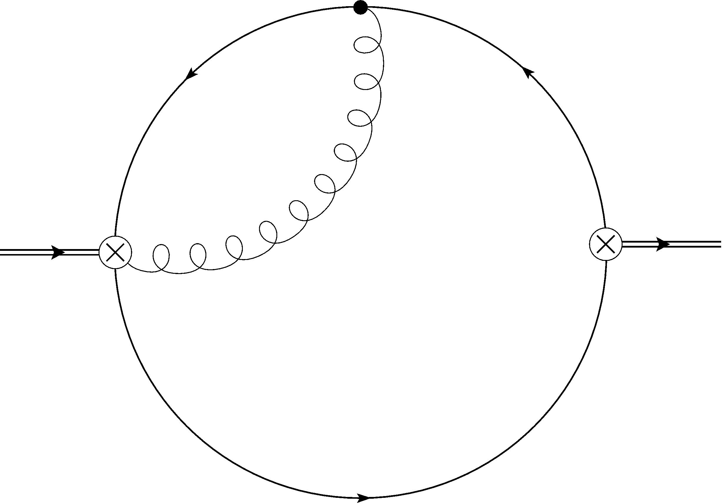
Diagram I
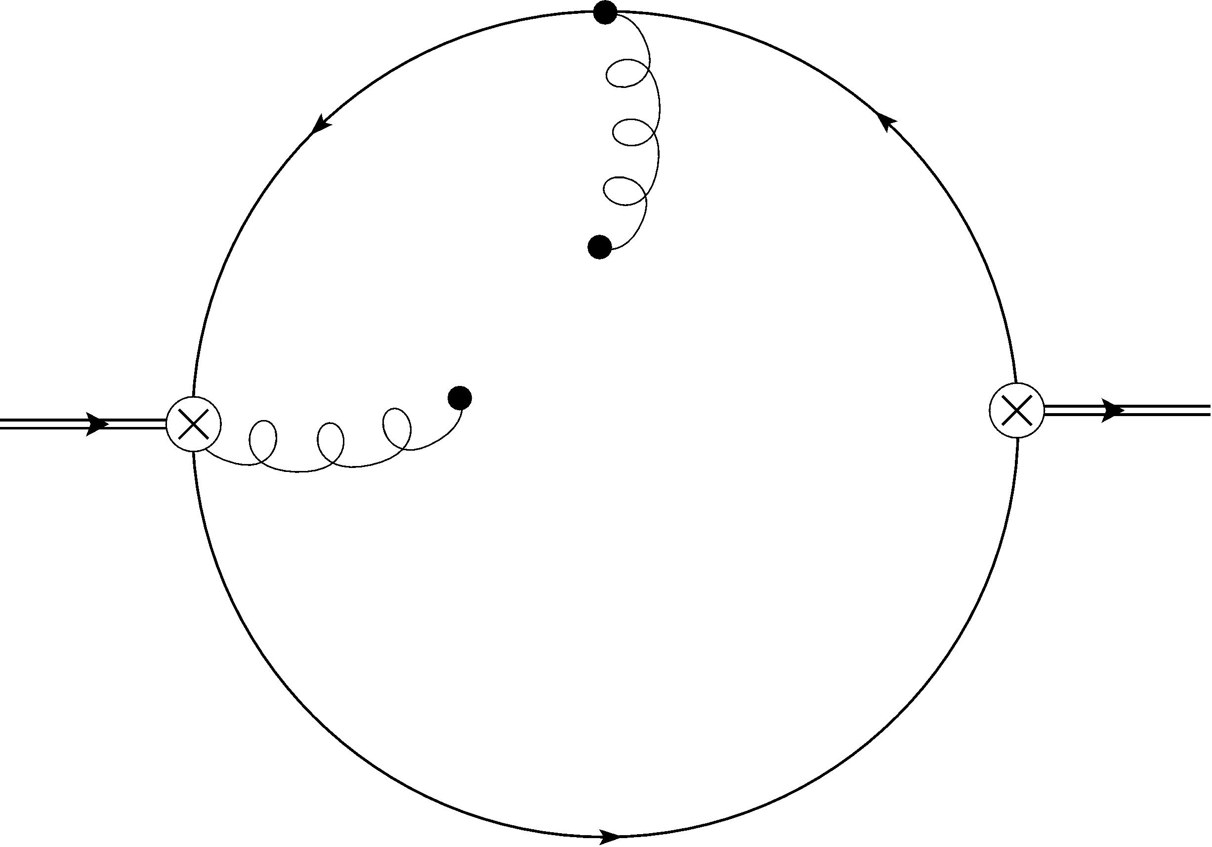
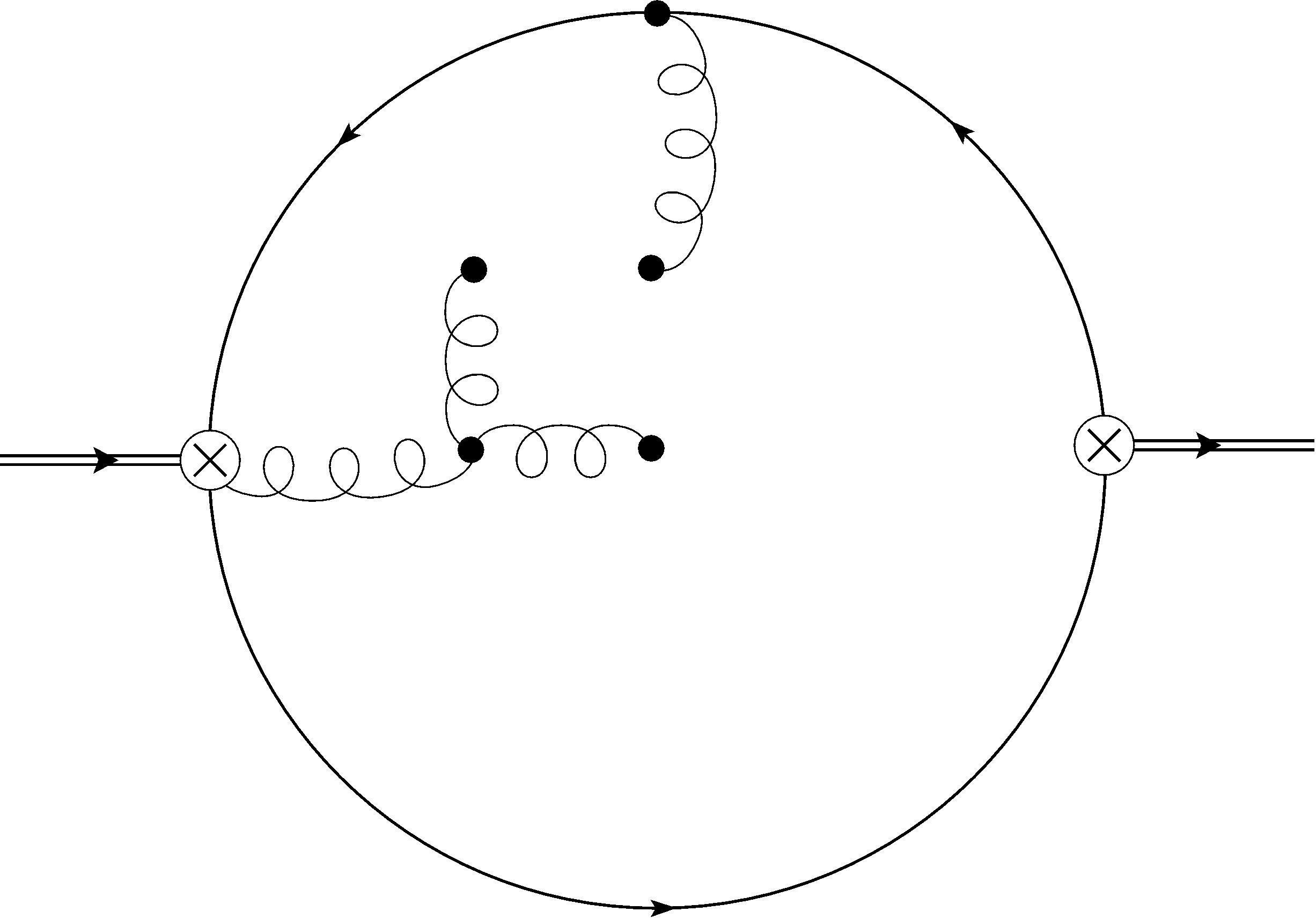
Diagram II	Diagram III
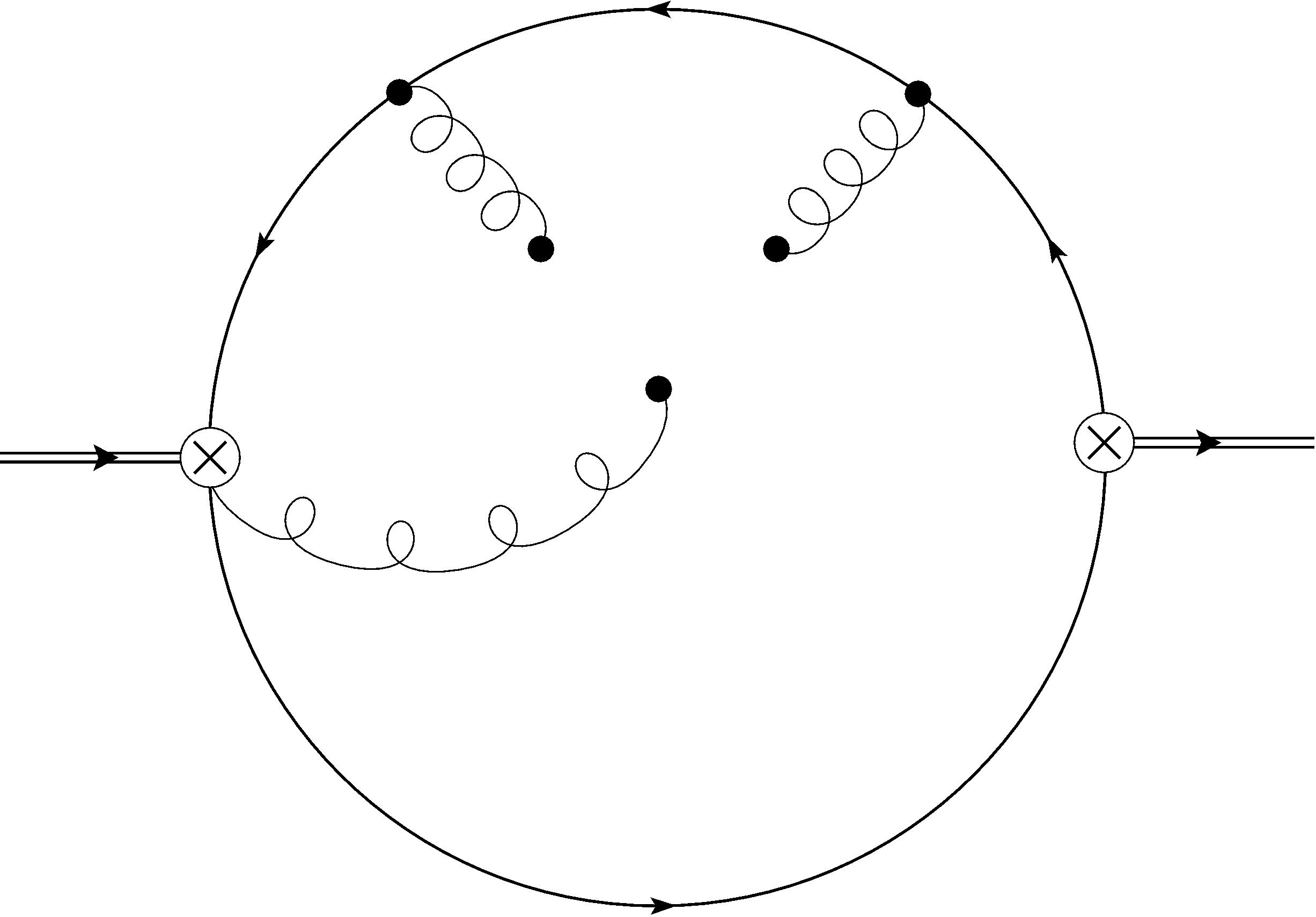
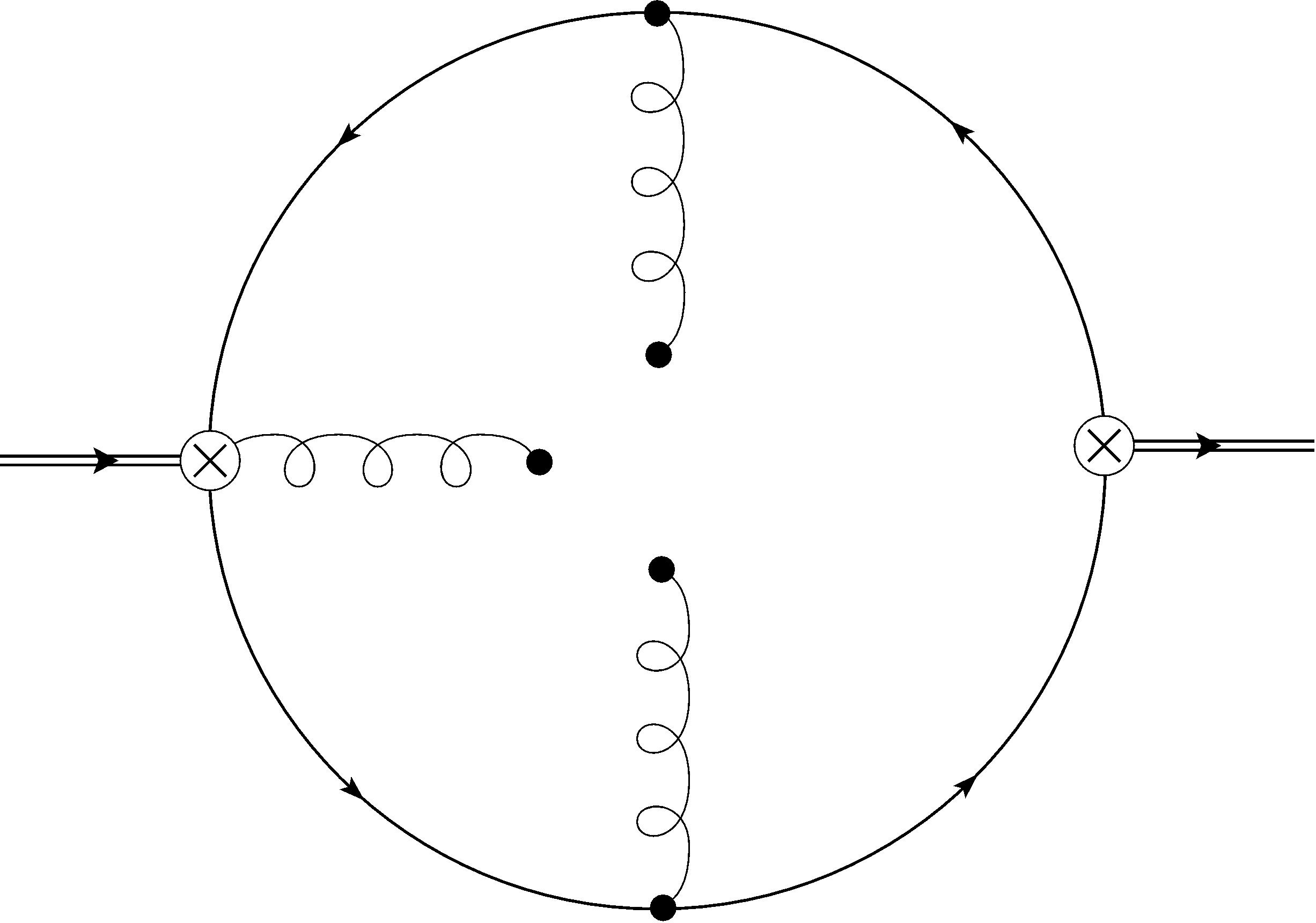
Diagram IV	Diagram V

Figure 1: The Feynman diagrams that contribute to (8)

Denoting the OPE calculation of $\Pi$ by $\Pi^{\text{OPE}}$, we decompose $\Pi^{\text{OPE}}$ as

$$\Pi^{\text{OPE}}=\Pi^{\text{I}}+\Pi^{\text{II}}+\Pi^{\text{III}}+\Pi^{\text{IV}}+\Pi^{\text{V}}$$ (8)

where the superscripts in (8) correspond to the labeling scheme of Figure 1. Expanding in $\epsilon$, we find

$$\Pi^{\text{I}}(q^{2})=\frac{2\alpha_{s}m^{4}z(1+4z)\>{}_{2}F_{1}\left(1,1;\frac{5}{2};z\right)}{9\pi^{3}}\frac{1}{\epsilon}+\cdots$$ (9)

$$\Pi^{\text{II}}(q^{2})=\frac{3z-z\;{}_{2}F_{1}\big{(}1,1;\frac{5}{2};z\big{)}}{18\pi(1-z)}\big{\langle}\alpha G^{2}\big{\rangle}$$ (10)

$$\begin{aligned} \Pi^{\text{III}}(q^{2})&=\frac{\big{\langle}g^{3}G^{3}\big{\rangle}}{1152\pi^{2}m^{2}(1-z)^{3}}\Bigg{(}-2-5z+4z^{2}\\ &\;\;+(2-7z+10z^{2}-4z^{3})\>{}_{2}F_{1}\big{(}1,1;\frac{5}{2};z\big{)}\Bigg{)}\end{aligned}$$ (11)

$$\begin{aligned} \Pi^{\text{IV}}(q^{2})&=\frac{\big{\langle}g^{3}G^{3}\big{\rangle}}{4608\pi^{2}m^{2}(1-z)^{3}}\Bigg{(}22-41z+16z^{2}\\ &\!\!\!-(10-25z+22z^{2}-8z^{3})\>{}_{2}F_{1}\big{(}1,1;\frac{5}{2};z\big{)}\Bigg{)}\end{aligned}$$ (12)

$$\begin{aligned} \Pi^{\text{V}}(q^{2})&=\frac{\big{\langle}g^{3}G^{3}\big{\rangle}}{1536\pi^{2}m^{2}(1-z)^{2}}\Bigg{(}-15+12z\\ &\;\;\;\;\;\;\;\;\;\;\;\;\;\;\;\;\;+(3-2z)\>{}_{2}F_{1}\big{(}1,1;\frac{5}{2};z\big{)}\Bigg{)}\end{aligned}$$ (13)

where $m$ is a heavy quark mass, $z=q^{2}/(4m^{2})$ and the ${}_{p}F_{q}(\cdots;\cdots;z)$ are generalized hypergeometric functions [21]. In (9) we include only a divergent term.

The perturbative result (9) contains a non-polynomial divergence which we eliminate via operator mixing under renormalization [11, 22]. The mesonic current (3) is renormalization-group (RG) invariant; thus, only operator mixing of the hybrid current (4) needs to be considered. Replacing the bare hybrid current (4) in (1) by

$$j_{\nu}^{(\text{h})}\rightarrow j_{\nu}^{(\text{h})}+\frac{C_{1}}{\epsilon}j_{\nu}^{(\text{m})}+\frac{C_{2}}{\epsilon}j_{\nu}^{(\text{c})}$$ (14)

where

$$j_{\nu}^{(c)}=\overline{Q}iD_{\nu}Q$$ (15)

and where $C_{1}$ and $C_{2}$ are as-yet-undetermined renormalization constants generates two renormalization-induced diagrams shown in Figure 2.

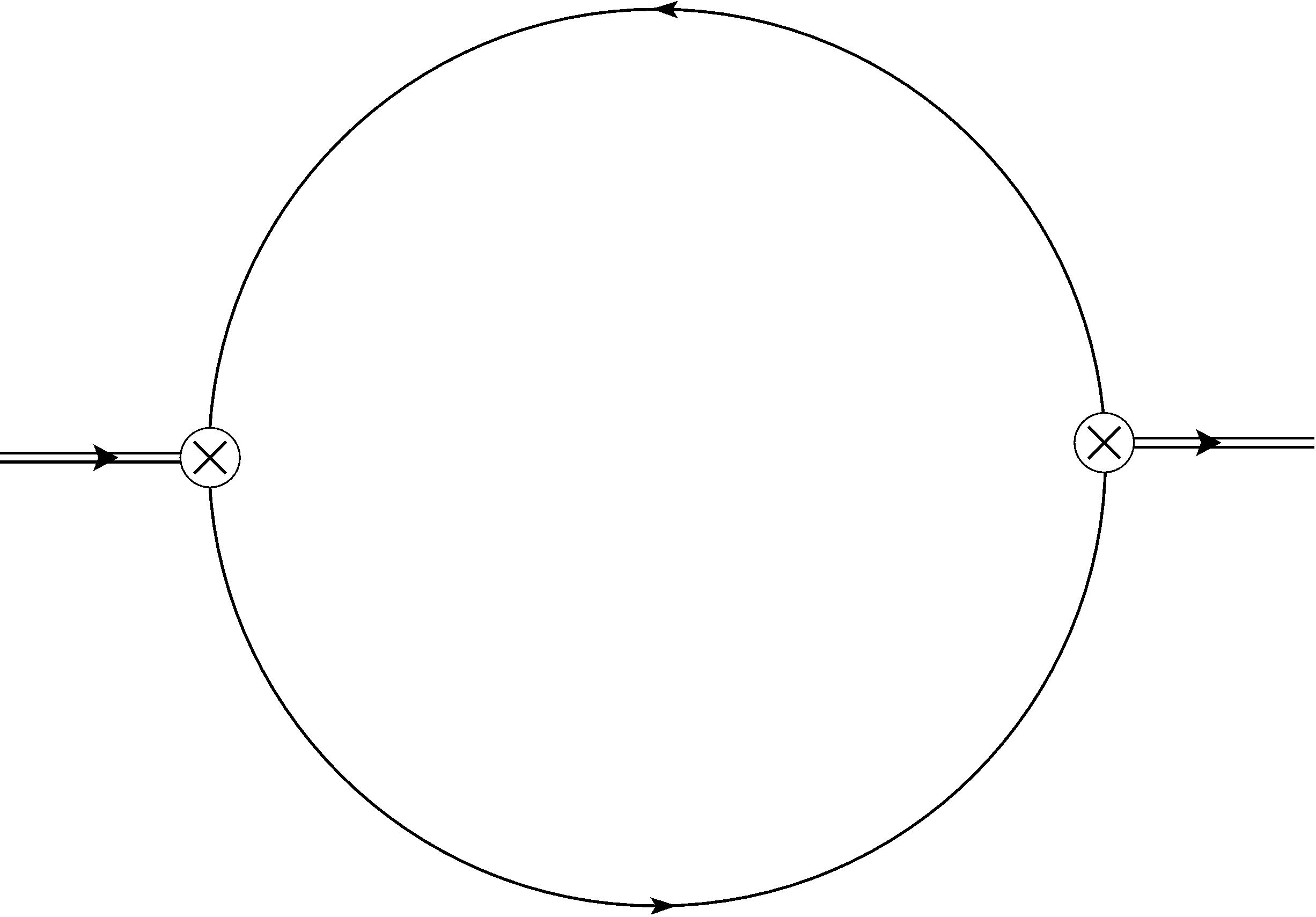
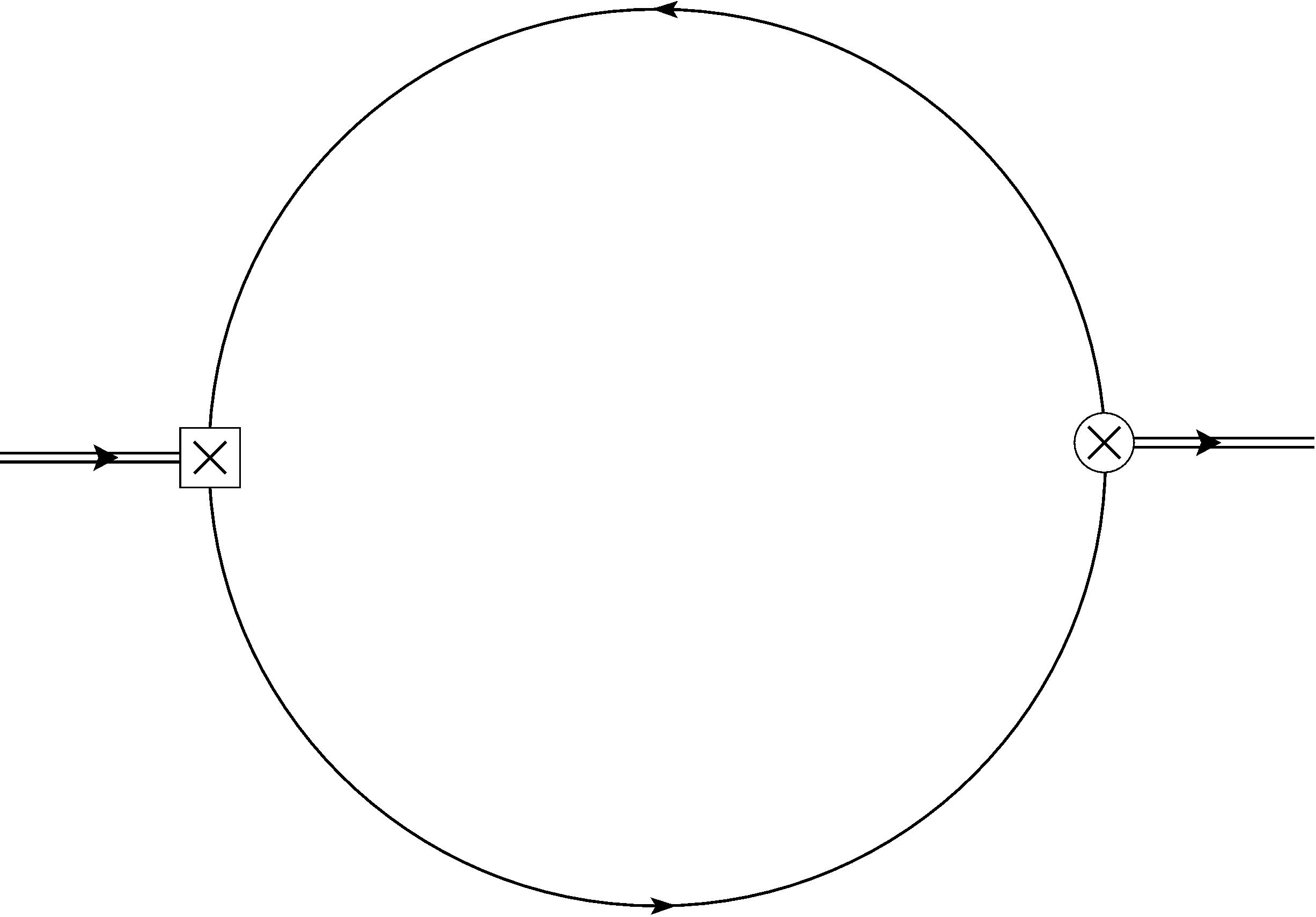
Figure 2: Renormalization-induced diagrams generated by (14), the square insertion represents current (15).

Evaluating these diagrams and choosing $C_{1}$ and $C_{2}$ such that the total perturbative contribution is divergences free, we find

$$C_{1}=-\frac{10m^{2}\alpha_{s}}{9\pi}\;\;\;\;\;\;\;\;\;C_{2}=\frac{4m\alpha_{s}}{9\pi}.$$ (16)

The updated perturbative result that replaces (9) is

$$\Pi^{(\text{I})}(q^{2})= \frac{2\alpha_{s}m^{4}z}{81\pi^{3}}\Bigg{(}18(z-1)\>{}_{3}F_{2}\big{(}1,1,1;\tfrac{3}{2},3;z\big{)}$$ (17)

$$-2z(4z+1)\>{}_{3}F_{2}\big{(}1,1,2;\tfrac{5}{2},4;z\big{)}$$

$$+3\Big{(}3(4z+1)\log\left(\frac{m^{2}}{\mu^{2}}\right)+26z+6\Big{)}$$

$$\;\;\;\;\;\;\;\times\>{}_{2}F_{1}\big{(}1,1;\tfrac{5}{2};z\big{)}\Bigg{)}.$$

In summary, $\Pi^{\text{OPE}}$ is the sum of (17) and (10) – (13).

3 QCD Laplace Sum-Rules

The correlator $\Pi$ defined in (2) satisfies the dispersion relation

$$\Pi(Q^{2})=\frac{Q^{6}}{\pi}\int_{t_{0}}^{\infty}\frac{\mathrm{Im}\Pi(t)}{t^{3}(t+Q^{2})}dt+\cdots$$ (18)

where $Q^{2}=-q^{2}>0$. On the left-hand side, we let $\Pi\to\Pi^{\text{OPE}}$; on the right-hand side, we identify $\mathrm{Im}\Pi(t)$ as the hadronic spectral function. To eliminate the subtraction constants in (18) represented by $\cdots$ and to accentuate the resonance contributions of the spectral function, we apply the Borel transform

$$\hat{\mathcal{B}}=\!\lim_{\stackrel{{\scriptstyle N,Q^{2}\rightarrow\infty}}{{\tau=N/Q^{2}}}}\!\frac{\big{(}-Q^{2}\big{)}^{N}}{\Gamma(N)}\bigg{(}\frac{d}{dQ^{2}}\bigg{)}^{N}$$ (19)

with Borel parameter $\tau$, and form the $0^{\text{th}}$-order LSR [5]

$$\mathcal{R}_{0}(\tau)\equiv\frac{1}{\tau}\hat{\mathcal{B}}\Big{\{}\Pi(Q^{2})\Big{\}}\\ =\int_{4m^{2}}^{\infty}e^{-t\tau}\frac{1}{\pi}\mathrm{Im}\Pi(t)dt.$$ (20)

We assume a resonance(s) plus continuum model

$$\frac{1}{\pi}\mathrm{Im}\Pi(t)=\rho^{\text{(had)}}(t)+\frac{1}{\pi}\mathrm{Im}\Pi^{\text{OPE}}(t)\theta(t-s_{0})$$ (21)

where $\rho^{\text{(had)}}$ represents the resonance portion of the spectral function and $s_{0}$ is the continuum threshold. (We discuss $\rho^{\text{(had)}}$ in Section 4.) Then, we define the continuum-subtracted $0^{\text{th}}$-order LSR as

$$\mathcal{R}_{0}(\tau,s_{0}) \equiv\mathcal{R}_{0}(\tau)-\int_{s_{0}}^{\infty}e^{-t\tau}\frac{1}{\pi}\mathrm{Im}\Pi^{\text{OPE}}(t)dt$$ (22)

$$=\int_{t_{0}}^{s_{0}}\rho^{\text{(had)}}(t)dt$$

where $t_{0}$ is the hadronic threshold.

To evaluate (22), we use the following relationship between the Borel transform and the inverse Laplace transform [5]

$$\frac{1}{\tau}\hat{\mathcal{B}}\Big{\{}f(Q^{2})\Big{\}} =\hat{\mathcal{L}}^{-1}\Big{\{}f(Q^{2})\Big{\}}$$ (23)

$$=\frac{1}{2\pi i}\int_{c-i\infty}^{c+i\infty}f(Q^{2})e^{Q^{2}\tau}dQ^{2}$$

where $c$ is a real constant for which $f(Q^{2})$ is analytic for $\text{Re}(Q^{2})>c$. The function $\Pi^{\text{OPE}}$ has a branch cut along the real axis for $Q^{2}<-4m^{2}$. Letting $f(Q^{2})\to\Pi^{\text{OPE}}(Q^{2})$ in (23) and warping the integration contour to that shown in Figure 3, we can write

$$\mathcal{R}_{0}(\tau,\,s_{0})= \int_{4m^{2}(1+\eta)}^{s_{0}}e^{-t\tau}\frac{1}{\pi}\text{Im}\Pi^{\text{OPE}}(t)\,dt$$ (24)

$$+\frac{1}{2\pi i}\int_{\Gamma_{\eta}}e^{Q^{2}\tau}\Pi^{\text{OPE}}(Q^{2})\,dQ^{2}$$

for $\eta\to 0^{+}$.

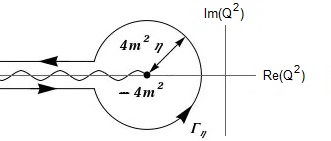
Figure 3: Integration contour used in the computation of the LSR (24)

RG improvement [23] requires that the strong coupling and quark mass in the LSR (24) get replaced by running quantities evaluated at renormalization scale $\mu$. At one-loop in $\overline{\text{MS}}$, we make the following replacements: for charmonium, we set $\mu\to\overline{m}_{c}$ in

$$\alpha_{s}(\mu)=\frac{\alpha_{s}(M_{\tau})}{1+\frac{25\alpha_{s}(M_{\tau})}{12\pi}\log\!{\Big{(}\frac{\mu^{2}}{M_{\tau}^{2}}\Big{)}}}$$ (25)

$$m_{c}(\mu)=\overline{m}_{c}\bigg{(}\frac{\alpha_{s}(\mu)}{\alpha_{s}(\overline{m}_{c})}\bigg{)}^{12/25}$$ (26)

whereas, for bottomonium, we set $\mu\to\overline{m}_{b}$ in

$$\alpha_{s}(\mu)=\frac{\alpha_{s}(M_{Z})}{1+\frac{23\alpha_{s}(M_{Z})}{12\pi}\log\!{\Big{(}\frac{\mu^{2}}{M_{Z}^{2}}\Big{)}}}$$ (27)

$$m_{b}(\mu)=\overline{m}_{b}\bigg{(}\frac{\alpha_{s}(\mu)}{\alpha_{s}(\overline{m}_{b})}\bigg{)}^{12/23}$$ (28)

where [24]

$$\alpha_{s}(M_{\tau})=0.330\pm 0.014$$ (29)

$$\alpha_{s}(M_{Z})=0.1185\pm 0.0006$$ (30)

$$\overline{m}_{c}=(1.275\pm 0.025)\ \text{GeV}$$ (31)

$$\overline{m}_{b}=(4.18\pm 0.03)\ \text{GeV}.$$ (32)

The condensate values used are [25, 26]

$$\big{\langle}\alpha G^{2}\big{\rangle}=(0.075\pm 0.02)\ \text{GeV}^{4}$$ (33)

$$\big{\langle}g^{3}G^{3}\big{\rangle}=(8.2\pm 1.0)\ \text{GeV}^{2})\,\big{\langle}\alpha G^{2}\big{\rangle}.$$ (34)

4 Analysis

We select a Borel window $(\tau_{\text{min}},\,\tau_{\text{max}})$ over which we will examine the LSR using the methodology of [11, 22, 27, 28]. We require that the LSR converges in the sense that the perturbative contribution is at least three times that of the 4d gluon condensate contribution which, in turn, is at least three times that of the 6d gluon condensate contribution. We also require that the resonance(s) contribution to the LSR is at least 10% that of the total resonance(s) plus continuum contributions i.e.,

$$\frac{\mathcal{R}_{0}(\tau,\,s_{0})}{\mathcal{R}_{0}(\tau,\,\infty)}>10\%.$$ (35)

We find that the Borel window for charmonium is $0.1\,\text{GeV}^{-2}\leq\tau\leq 0.6\,\text{GeV}^{-2}$ and for bottomonium is $0.01\,\text{GeV}^{-2}\leq\tau\leq 0.2\,\text{GeV}^{-2}$.

The quantity $\rho^{\text{(had)}}$ in (21) will contain resonances that are to be tested for coupling to both the meson (3) and hybrid (4) currents. The vector charmonium and bottomonium resonances listed by the Particle Data Group [24] are summarized in Table 1.

Table 1: Heavy vector quarkonium resonances.

Charmonium Name Mass (GeV) $J/\psi$ 3.10 $\psi(2S)$ 3.69 $\psi(3770)$ 3.77 $\psi(4040)$ 4.04 $\psi(4160)$ 4.19 $X(4230)$ 4.23 $X(4260)$ 4.23 $X(4360)$ 4.34 $\psi(4415)$ 4.42 $X(4660)$ 4.64	Bottomonium Name Mass (GeV) $\Upsilon(1S)$ 9.46 $\Upsilon(2S)$ 10.02 $\Upsilon(3S)$ 10.34 $\Upsilon(4S)$ 10.58 $\Upsilon(10860)$ 10.89 $\Upsilon(11020)$ 10.99
Note: in the charmonium sector entries labeled with $X$ are those with unknown $I^{G}$ whereas $\psi$ indicates $I^{G}=0^{-}$.

All resonances in Table 1 have widths of $\lesssim 100$ MeV. As LSRs are quite insensitive to resonance width, we ignore the widths of individual resonances. For collections of resonances with masses separated by 250 MeV or less, we cluster these resonances into a single resonance with nonzero (or, in some models, zero) width. We consider a variety of $\rho^{\text{(had)}}$ of the form

$$\rho^{\text{(had)}}(t)=\sum_{i=1}^{n}\begin{cases}\xi_{i}\delta(t-m_{i}^{2}),\ \Gamma_{i}=0\\ \frac{\xi_{i}}{2m_{i}\Gamma_{i}}\theta\big{(}t-m_{i}(m_{i}-\Gamma_{i})\big{)}\\ \;\;\;\times\;\theta\big{(}m_{i}(m_{i}+\Gamma_{i})-t\big{)},\ \Gamma_{i}\neq 0\end{cases}$$ (36)

where $n$ is the number of distinct resonances or resonance clusters and $\Gamma_{i}$ are the resonance cluster widths. The quantities $\xi_{i}$ are mixing parameters. Resonances with both meson and hybrid components (i.e., mixed states) have $\xi_{i}\neq 0$; pure meson or pure hybrid states have $\xi_{i}=0$. Substituting (36) into (22) gives

$$\mathcal{R}_{0}(\tau,\,s_{0})=\sum_{i=1}^{n}\begin{cases}\xi_{i}e^{-m_{i}^{2}\tau},\ \Gamma_{i}=0\\ \xi_{i}e^{-m_{i}^{2}\tau}\frac{\sinh\big{(}m_{i}\Gamma_{i}\tau\big{)}}{m_{i}\Gamma_{i}\tau},\ \Gamma_{i}\neq 0\end{cases}\!\!\!\!.$$ (37)

Informed by Table 1, we input a variety of choices for $m_{i}$ and $\Gamma_{i}$ into (37). We then partition the Borel window $(\tau_{\text{min}},\,\tau_{\text{max}})$ into $N=20$ equal length subintervals using grid points $\{\tau_{j}\}_{j=0}^{N}$ and define

$$\chi^{2}(\xi_{1}, \ldots,\xi_{n},\,s_{0})=$$ (38)

$$\!\!\sum_{j=0}^{N}\Bigg{(}\mathcal{R}_{0}(\tau_{j},\,s_{0})-\sum_{i=1}^{n}\int_{4m^{2}}^{s_{0}}e^{-t\tau_{j}}\rho^{\text{(had)}}_{i}(t)dt\Bigg{)}^{2}.$$

By minimizing (38), we extract $\xi_{i}$ and $s_{0}$ as best-fit parameters. Table 2 contains the models used and results obtained in the charmonium sector, and Table 3 contains similar information for the bottomonium sector. Rather than present each $\xi_{i}$, we instead present $\zeta$ and $\frac{\xi_{i}}{\zeta}$ where

$$\zeta=\sum_{i=1}^{n}|\xi_{i}|.$$ (39)

The errors in Tables 2 and 3 include a variation of $\pm 0.1$ GeV in the renormalization scale $\mu$. We also vary the end points of the Borel window by $\pm 0.05\ \text{GeV}^{-2}$ in the charmonium analysis and by $\pm 0.005\ \text{GeV}^{-2}$ in the bottomonium analysis. Additionally, we include the errors associated with the quantities (29) – (34). Our results are most sensitive to uncertainties in the quark mass parameters (31) and (32).

5 Discussion

Looking at the $\chi^{2}$ values in Tables 2 and 3, we see that the inclusion of a third heavy resonance cluster in our models significantly improves the fits. Note that these third resonance clusters make large contributions to the LSR in spite of the LSR’s suppression of higher mass resonance contributions. Consider a quantitative measure of the third resonance’s contribution given by

$$\frac{\int_{t_{0}}^{s_{0}}e^{-t\tau}\rho_{3}^{(\text{had})}(t)dt}{\sum_{i=1}^{3}\left|\int_{t_{0}}^{s_{0}}e^{-t\tau}\rho_{i}^{(\text{had})}(t)dt\right|}.$$ (40)

For example, evaluating (40) for Model C3 of Table 2 gives $0.43$. In the bottomonium sector, Model B3 of Table 3 gives $0.35$. The $\chi^{2}$ values also indicate that the inclusion of resonance widths (i.e., $\Gamma_{i}\neq 0$) has no significant impact on the fits. This insensitivity to resonance width is a characteristic of LSRs and is expected.

Models including a fourth resonance were also examined, but, in all cases, led to $\chi^{2}$ minima occurring at $s_{0}\!\approx\!m_{4}^{2}$. In other words, these fourth resonances merged with the continuum in contradiction with the separation between resonances and continuum assumed in (21). Furthermore, the two resonance models examined in Tables 2 and 3 (i.e., Models C2 and B2) suffer from this same problem making them too unreliable.

Examining the three resonance models in the charmonium sector (Models C3, C4 and C5), we find a nonzero mixing parameter for the $J/\psi$; no evidence for mixing in the $\psi(2S),\,\psi(3770)$ cluster; and a large mixing parameter for the $4.3$ GeV cluster. This $4.3$ GeV cluster represents a grouping of all resonances from the $\psi(4040)$ to the $X(4660)$. The effects of varying $m_{3}$ in this system from 4.0 GeV–4.6 GeV were investigated, and we found that $m_{3}=4.3$ GeV yielded the smallest minimum $\chi^{2}$ value. As the $\psi(2S),\,\psi(3770)$ cluster exhibits no mixing, the final two models in Table 2 (Models C6 and C7) exclude this cluster; doing so has minimal effect on the values of $\xi_{1},\ \xi_{3},s_{0}$ and the minimum value of $\chi^{2}$.

In the bottomonium sector, the three resonance models in Table 3 (Models B3 and B4) show a nonzero mixing parameter for all three resonances. Thus, the $\Upsilon(1S)$, $\Upsilon(2S)$, and $\Upsilon(3S),\,\Upsilon(4S)$ cluster all exhibit mixing.

To summarize, in both the charmonium and bottomonium sectors, we find that the addition of a third heavy resonance cluster improves the agreement between theory and experiment significantly. In the charmonium sector, meson-hybrid mixing is well-described by a two resonance model consisting of the $J/\psi$ and a second state with mass $\approx 4.3$ GeV. This result is consistent with the hypothesis that the $X(4260)$ could be a resonance with significant hybrid content [29, 30, 31]. In the bottomonium sector, our results indicate nonzero mixing in the $\Upsilon(1S)$, $\Upsilon(2S)$, and $\Upsilon(3S),\,\Upsilon(4S)$ cluster.

Acknowledgements- We are grateful for financial support from the Natural Sciences and Engineering Research Council of Canada (NSERC).

Table 2: Models and results in the charmonium sector

Model	$m_{1}$ , $\Gamma_{1}$	$m_{2}$ , $\Gamma_{2}$	$m_{3}$ , $\Gamma_{3}$	$s_{0}$	$\chi^{2}\times 10^{6}$	$\zeta$	$\frac{\xi_{1}}{\zeta}$	$\frac{\xi_{2}}{\zeta}$	$\frac{\xi_{3}}{\zeta}$
#	(GeV)	(GeV)	(GeV)	(GeV2)	(GeV12)	(GeV6)
C1	3.10 , 0	-	-	12.4	3.32	$0.507\pm 0.022$	1	$-$	$-$
C2	3.10 , 0	3.73 , 0	-	13.9	2.23	$0.736\pm 0.043$	$0.716\pm 0.035$	$\;\;\,0.284\pm 0.035$	$-$
C3	3.10 , 0	3.73 , 0	4.30 , 0	23.7	0.105	$2.679\pm 0.254$	$0.224\pm 0.014$	$0.010\pm 0.055$	$0.766\pm 0.042$
C4	3.10 , 0	3.73 , 0	4.30 , 0.30	23.8	0.103	$2.709\pm 0.274$	$0.222\pm 0.015$	$-0.001\pm 0.054$	$0.777\pm 0.044$
C5	3.10 , 0	3.73 , 0.05	4.30 , 0.30	23.8	0.103	$2.709\pm 0.274$	$0.222\pm 0.015$	$-0.001\pm 0.054$	$0.777\pm 0.044$
C6	3.10 , 0	-	4.30 , 0	23.9	0.109	$2.713\pm 0.263$	$0.223\pm 0.019$	$-$	$0.777\pm 0.019$
C7	3.10 , 0	-	4.30 , 0.30	23.8	0.103	$2.699\pm 0.262$	$0.223\pm 0.020$	$-$	$0.777\pm 0.020$

Table 3: Models and results in the bottomonium sector

Model	$m_{1}$ , $\Gamma_{1}$	$m_{2}$ , $\Gamma_{2}$	$m_{3}$ , $\Gamma_{3}$	$s_{0}$	$\chi^{2}\times 10^{4}$	$\zeta$	$\frac{\xi_{1}}{\zeta}$	$\frac{\xi_{2}}{\zeta}$	$\frac{\xi_{3}}{\zeta}$
#	(GeV)	(GeV)	(GeV)	(GeV2)	(GeV12)	(GeV6)
B1	9.46 , 0	-	-	105	169	$132\pm 4$	1	$-$	$-$
B2	9.46 , 0	10.02 , 0	-	100	154	$165\pm 8$	$0.824\pm 0.015$	$-0.176\pm 0.015$	$-$
B3	9.46 , 0	10.02 , 0	10.47 , 0	130	0.18	$1255\pm 83$	$0.213\pm 0.004$	$-0.374\pm 0.006$	$0.413\pm 0.004$
B4	9.46 , 0	10.02 , 0	10.47 , 0.22	130	0.18	$1259\pm 83$	$0.212\pm 0.004$	$-0.375\pm 0.006$	$0.413\pm 0.004$

References

- [1] N. Brambilla, et al., Heavy quarkonium: progress, puzzles, and opportunities, Eur. Phys. J. C71 (2011) 1534. arXiv:1010.5827, doi:10.1140/epjc/s10052-010-1534-9.
- [2] S. Eidelman, B. K. Heltsley, J. J. Hernandez-Rey, S. Navas, C. Patrignani, Developments in heavy quarkonium spectroscopyarXiv:1205.4189.
- [3] M. Ablikim, et al., Evidence of Two Resonant Structures in , Phys. Rev. Lett. 118 (9) (2017) 092002. arXiv:1610.07044, doi:10.1103/PhysRevLett.118.092002.
-
[4]
T. Barnes, F. E. Close, E. S. Swanson,
Hybrid and conventional
mesons in the flux tube model: Numerical studies and their phenomenological
implications, Phys. Rev. D52 (1995) 5242–5256.
doi:doi:10.1103/PhysRevD.52.5242.
URL http://arxiv.org/pdf/hep-ph/9501405v2.pdf - [5] M. A. Shifman, A. I. Vainshtein, V. I. Zakharov, QCD and Resonance Physics. Theoretical Foundations, Nucl. Phys. B147 (1979) 385–447. doi:10.1016/0550-3213(79)90022-1.
- [6] M. A. Shifman, A. I. Vainshtein, V. I. Zakharov, QCD and Resonance Physics: Applications, Nucl. Phys. B147 (1979) 448–518. doi:10.1016/0550-3213(79)90023-3.
- [7] L. J. Reinders, H. Rubinstein, S. Yazaki, Hadron Properties from QCD Sum Rules, Phys. Rept. 127 (1985) 1. doi:10.1016/0370-1573(85)90065-1.
- [8] S. Narison, QCD as a Theory of Hadrons, Vol. 17 of Cambridge Monographs on Particle Physics, Nuclear Physics and Cosmology, Cambridge University Press, New York, 2004.
- [9] S. Narison, N. Pak, N. Paver, Meson - Gluonium Mixing From QCD Sum Rules, Phys. Lett. 147B (1984) 162, [,77(1984)]. doi:10.1016/0370-2693(84)90613-0.
- [10] D. Harnett, R. T. Kleiv, K. Moats, T. G. Steele, Near-Maximal Mixing of Scalar Gluonium and Quark Mesons: A Gaussian Sum-Rule Analysis, Nucl. Phys. A850 (2011) 110–135. arXiv:0804.2195, doi:10.1016/j.nuclphysa.2010.12.005.
- [11] W. Chen, H.-y. Jin, R. T. Kleiv, T. G. Steele, M. Wang, Q. Xu, QCD sum-rule interpretation of X(3872) with mixtures of hybrid charmonium and molecular currents, Phys. Rev. D88 (4) (2013) 045027. arXiv:1305.0244, doi:10.1103/PhysRevD.88.045027.
- [12] J. Govaerts, L. J. Reinders, J. Weyers, Radial excitations and exotic mesons via QCD sum rules, Nucl. Phys. B262 (1985) 575. doi:doi:10.1016/0550-3213(85)90505-X.
- [13] P. Pascual, R. Tarrach, QCD: Renormalization for the Practitioner, Springer, 1984.
- [14] E. Bagán, M. R. Ahmady, V. Elias, T. G. Steele, plane-wave, coordinate-space, and moment techniques in the operator-product expansion: equivalence, improved methods, and the heavy quark expansion, Z. Phys. C61 (1994) 157–170.
- [15] D. A. Akyeampong, R. Delbourgo, dimensional regularization, abnormal amplitudes, and anomalies, Nuovo Cim. 17 (1973) 578.
- [16] R. Mertig, R. Scharf, TARCER - a Mathematica program for the reduction of two-loop propagator integrals, Comput. Phys. Commun. 111 (1998) 265–273.
- [17] O. V. Tarasov, Connection between feynman integrals having different values of the space-time dimension, Phys. Rev. D54 (1996) 6479–6490.
- [18] O. V. Tarasov, Generalized recurrence relations for two-loop propagator integrals with arbitrary masses, Nucl. Phys. B502 (1997) 455–482.
- [19] E. E. Boos, A. I. Davydychev, A method of evaluating massive feynman integrals, Theor. Math. Phys. 89 (1991) 1052–1063.
- [20] D. J. Broadhurst, J. Fleischer, O. V. Tarasov, Two-loop two-point functions with masses: asymptotic expansions and taylor series, in any dimension, Z. Phys. C60 (1993) 287–302.
- [21] M. Abramowitz, I. A. Stegun, Handbook of Mathematical Functions, Dover Publications, 1965.
- [22] J. Ho, D. Harnett, T. G. Steele, Masses of open-flavour heavy-light hybrids from QCD sum-rules, JHEP (2017) In Press.
- [23] S. Narison, E. de Rafael, On QCD Sum Rules of the Laplace Transform Type and Light Quark Masses, Phys. Lett. B103 (1981) 57–62. doi:10.1016/0370-2693(81)90193-3.
- [24] C. Patrignani, et al., Review of Particle Physics, Chin. Phys. C40 (10) (2016) 100001. doi:10.1088/1674-1137/40/10/100001.
- [25] G. Launer, S. Narison, R. Tarrach, Nonperturbative QCD Vacuum From I = 1 Hadron Data, Z. Phys. C26 (1984) 433–439. doi:10.1007/BF01452571.
- [26] S. Narison, Gluon condensates and c, b quark masses from quarkonia ratios of moments, Phys. Lett. B693 (2010) 559–566. doi:doi:10.1016/j.physletb.2011.09.116.
-
[27]
R. Berg, D. Harnett, R. T. Kleiv, T. G. Steele,
Mass predictions for pseudoscalar
charmonium and bottomonium hybrids in QCD sum-rules, Phys.
Rev. D86 (2012) 034002.
doi:doi:10.1103/PhysRevD.86.034002.
URL http://arxiv.org/pdf/1204.0049.pdf - [28] D. Harnett, R. T. Kleiv, T. G. Steele, H.-y. Jin, Axial Vector Charmonium and Bottomonium Hybrid Mass Predictions with QCD Sum-Rules, J. Phys. G39 (2012) 125003. arXiv:1206.6776, doi:10.1088/0954-3899/39/12/125003.
-
[29]
F. E. Close, P. R. Page, The
photoproduction of hybrid mesons from cebaf to hera, Phys. Rev. D52 (1995)
1706–1709.
doi:doi:10.1103/PhysRevD.52.1706.
URL http://arxiv.org/pdf/hep-ph/9412301v1.pdf - [30] E. Kou, O. Pene, Suppressed decay into open charm for the Y(4260) being an hybrid, Phys. Lett. B631 (2005) 164–169. arXiv:hep-ph/0507119, doi:10.1016/j.physletb.2005.09.013.
- [31] S.-L. Zhu, The Possible interpretations of Y(4260), Phys. Lett. B625 (2005) 212. arXiv:hep-ph/0507025, doi:10.1016/j.physletb.2005.08.068.