Exploring High-order three dimensional Virtual Elements: bases and stabilizations

Abstract

We present numerical tests of the Virtual Element Method (VEM) tailored for the discretization of a three dimensional Poisson problem with high-order “polynomial” degree (up to $p=10$). Besides, we discuss possible reasons for which the method could return suboptimal-wrong error convergence curves. Among these motivations, we highlight ill-conditioning of the stiffness matrix and not particularly “clever” choices of the stabilizations. We propose variants of the definition of face/bulk degrees of freedom, as well as of stabilizations, which lead to methods that are much more robust in terms of numerical performances.

Keywords: Virtual Element Method, Polyhedral meshes, high-order methods, ill-conditioning

1 Introduction

The Virtual Element Method (VEM) is a generalization of the Finite Element Method (FEM) that allows for general polytopal meshes, thus including non-convex elements and hanging nodes.

Approximation spaces in VEM contain locally polynomials and, more in general, consist of functions which solve local problems mimicking the original ones and, consequently, are not known in a closed form (hence the name virtual). For this reason, the operators involved in the discretization of the problem are not computed exactly; rather, the construction of the method is based on two ingredients: proper projectors onto piecewise discontinuous polynomial spaces and stabilizing bilinear forms mimicking their continuous counterparts. Both ingredients can be computed exactly only with the aid of the degrees of freedom.

Although the VEM technology is very recent, it has been applied to a large number of two dimensional problems; a short of list of them is: [1, 6, 12, 7, 13, 5, 20]; in particular, high-order VEM are investigated in [9, 10, 2, 14, 19].

The literature dealing with three dimensional problems is much less broad, see [18, 17, 15]. The only attempt, at the best of our knowledge, to increase the order of VEM in 3D is [11], where the highest order achieved in numerical tests is $p=5$.

In the present work, we have a double aim. Firstly, we present numerical tests for three dimensional VEM of order higher than $5$, thus inviting the reader to raise the anchor from the safe port [11] and to “…Walk out with us toward the Unknown Region…”, reaching in fact the pinnacle of degree of accuracy $p=10$. Secondly, we numerically investigate the reasons of possible suboptimal/wrong behaviour in the error convergence curves, highlighting two among them: the ill-conditioning of the linear system stemming from the method and the choice of the stabilization.

We tackle the (possible) issue of suboptimality of VEM, when considering its $h$ and $p$ versions as well as when it is applied to meshes with elements having collapsing bulk, by proposing two novel approaches of the definition of the face/bulk degrees of freedom and proposing three different stabilizations.

The outline of the paper follows. In Section 2, we review the construction of three dimensional VEM, emphasizing in particular different stabilizations and face/bulk degrees of freedom. Next, in Section 3, we provide a number of numerical results comparing the effects on the method of the above-mentioned stabilizations and degrees of freedom; more precisely, we study the $h$ and the $p$ versions of the method, paying attention also to VEM applied to meshes with degenerate elements. Concluding remarks are stated in Section 4. Finally, in Appendix A, we give some hints regarding the implementation of the method with the novel canonical basis functions.

Notation.

By $\mathbb{P}_{p}(F)$ and $\mathbb{P}_{p}(K)$, $p\in\mathbb{N}$, we denote the spaces of two and three dimensional polynomials of degree $p$ over a polygon $F$ and a polyhedron $K$, respectively; if $p=-1$, then we set $\mathbb{P}_{-1}(F)=\mathbb{P}_{-1}(K)=\emptyset$. Moreover, we fix:

$$n_{p}^{F}=\dim(\mathbb{P}_{p}(F)),\quad\quad n_{p}=\dim(\mathbb{P}_{p}(K))\quad\forall\,p\in\mathbb{N}.$$ (1)

Assume now that we are given $\{m_{\alpha}\}_{\alpha=1}^{n_{p}}$, $p\in\mathbb{N}$, a basis of $\mathbb{P}_{p}(K)$ such that:

$$\text{span}\left(\{m_{\alpha}\}_{\alpha=1}^{n_{p-2}}\right)=\mathbb{P}_{p-2}(K)\quad\text{and }\quad\text{span}\left(\{m_{\alpha}\}_{\alpha=1}^{n_{p-1}}\right)=\mathbb{P}_{p-1}(K).$$ (2)

It will be convenient to split the polynomial basis into:

$$\{m_{\alpha}\}_{\alpha=1}^{n_{p}}=\{m_{\alpha}\}_{\alpha=1}^{n_{p-2}}\cup\{m_{\alpha}\}_{\alpha=n_{p-2}+1}^{n_{p-1}}\cup\{m_{\alpha}\}_{\alpha=n_{p-1}+1}^{n_{p}}.$$ (3)

We assume that the polygonal counterpart of (2) holds true; consequently, we can consider a splitting analogous to the one in (3) on

$$\mathbb{P}_{p}(F)=\text{span}\left(\{m_{\alpha}^{F}\}_{\alpha=1}^{n_{p}^{F}}\right),$$

the space of polynomial of degree $p$ over polygon $F$.

2 VEM: definition, stabilizations and bases

In this section, we introduce a family of VEM tailored for the approximation of the following Poisson problem in three dimensions with (for simplicity) homogeneous boundary conditions. Given $\Omega\subset\mathbb{R}^{3}$ a polyhedral domain and $f\in L^{2}(\Omega)$:

$$\begin{cases}\text{find }u\in V\text{ s. th.}\\ a(u,v)=(f,v)\quad\forall\,v\in V\end{cases},$$ (4)

where:

$$V=H^{1}_{0}(\Omega),\quad\quad a(\cdot,\cdot)=(\nabla\cdot,\nabla\cdot)_{0,\Omega}.$$ (5)

In Section 2.1, we briefly recall from [1, 11, 8] the construction of three dimensional VEM for the approximation of the solution of problem (4), keeping yet at a very general level the definition of the degrees of freedom and of the stabilization of the method, typical of the VEM framework. Various choices of stabilizations as well as of face/bulk degrees of freedom are investigated in Sections 2.2 and 2.3, respectively.

2.1 A family of VEM

In this section, we introduce, following [1, 11], a family of VEM in three dimensions for the approximation of problem (4).

The VEM in three dimensions is based on conforming sequences $\mathcal{T}_{n}$ of polyhedra partitioning the physical domain $\Omega$ of the PDE of interest. By conforming sequence, we mean that, given $\mathcal{F}_{n}$, $\mathcal{E}_{n}$ and $\mathcal{V}_{n}$ the sets of all faces, edges and vertices of the polyhedra in $\mathcal{T}_{n}$, respectively, then all the internal faces $F\in\mathcal{F}_{n}$ must belong to the intersection of two polyhedra.

We observe that, since the aim of the present paper is to test the robustness of the method to mesh-distortion and to increasing “polynomial degrees”, no particular geometrical assumptions on the mesh are demanded.

Let now $p\in\mathbb{N}$; such $p$ denotes the “polynomial degree” of the method. We begin by defining the local spaces on each face $F\in\mathcal{F}_{n}$:

$$\widetilde{V}_{p}(F)=\{v_{p}\in H^{1}(F)\mid\Delta v_{p}\in\mathbb{P}_{p}(F),\,v_{p}|_{\partial F}\in\mathbb{B}_{p}(\partial F)\},$$ (6)

where:

$$\mathbb{B}_{p}(\partial F)=\{v_{p}\in\mathcal{C}^{0}(\partial F)\mid v_{p}|_{s}\in\mathbb{P}_{p}(s)\text{ for all edges }s\text{ of }F\}.$$ (7)

Given any polynomial basis $\{m_{\alpha}^{F}\}_{\alpha=1}^{n_{p-2}^{F}}$ of $\mathbb{P}_{p-2}(F)$ satisfying the face counterpart of (2), we can endow space (6) with the following set of linear functionals. For every $v_{p}\in\widetilde{V}_{p}(F)$:

• the values of $v_{p}$ at the vertices of $F$;

• the values of the $p-1$ internal Gauß-Lobatto nodes on each edge $s$ of face $F$;

• the (scaled) face moments:

  $$\frac{1}{|F|}\int_{F}m_{\alpha}^{F}\,v_{p}\quad\quad\forall\,\alpha=1,\dots,n_{p-2}^{F}.$$ (8)

It can be proven, see [4], that it is possible to compute via such linear functionals the energy projector $\Pi^{\nabla,F}_{p}:\widetilde{V}_{p}(F)\rightarrow\mathbb{P}_{p}(F)$ defined as:

$$\begin{cases}\vskip 6.0pt plus 2.0pt minus 2.0pt(\nabla q_{p}^{F},\nabla(v_{p}-\Pi^{\nabla,F}_{p}v_{p}))_{0,F}=:a^{F}(q_{p}^{F},v_{p}-\Pi^{\nabla,F}_{p}v_{p})=0\\ \vskip 6.0pt plus 2.0pt minus 2.0pt\begin{cases}\sum_{i=1}^{N_{V}^{F}}(v_{p}-\Pi^{\nabla,F}_{p}v_{p})(\nu_{i}^{F})=0&\text{if }p=1\\ \int_{F}v_{p}-\Pi^{\nabla,F}_{p}v_{p}=0&\text{if }p\geq 2\\ \end{cases}\end{cases}\quad\forall\,q_{p}^{F}\in\mathbb{P}_{p}(F),\,\forall\,v_{p}\in\widetilde{V}_{p}(F),\\$$ (9)

where $N_{V}^{F}$ and $\{\nu_{i}^{F}\}_{i=1}^{N_{V}^{F}}$ denotes the number and the set of vertices of face $F$, respectively.

Following now [1], we restrict space $\widetilde{V}_{p}(F)$ defined in (6) so that one is able to compute an $L^{2}$ projector onto $\mathbb{P}_{p}(F)$ via the set of linear functionals introduced above.

Such a space, which goes under the name of “enhanced VE planar space”, is defined as:

$$V_{p}(F)=\left\{v_{p}\in\widetilde{V}_{p}(F)\,\left|\,\int_{F}(v_{p}-\Pi^{\nabla,F}_{p}v_{p})m_{\alpha}^{F},\,\text{for all }\alpha=n_{p-2}^{F}+1,\dots,n_{p}^{F}\right.\right\},$$ (10)

see (3) for the splitting of the polynomial basis.

As already stressed, it is possible to compute on such space, in addition the the energy projector defined in (9), the $L^{2}$ projector $\Pi^{0,F}_{p}:V_{p}(F)\rightarrow\mathbb{P}_{p}(F)$ defined as:

$$(q_{p}^{F},v_{p}-\Pi^{0,F}_{p}v_{p})_{0,F}=0\quad\forall\,q_{p}^{F}\in\mathbb{P}_{p}(F),\,\forall\,v_{p}\in V_{p}(F).$$ (11)

Remark 1.

We observe that the definition of space (10) and of the $H^{1}$ and $L^{2}$ orthogonal projectors are independent of the choice of the polynomial basis employed in the definition of face moments (8).

At this point, we are in business for defining local VE spaces on polyhedra. We begin also in this case by introducing an auxiliary space:

$$\widetilde{V}_{p}(K)=\left\{v_{p}\in H^{1}(K)\mid\Delta v_{p}\in\mathbb{P}_{p}(K),\,v_{p}|_{F}\in V_{p}(F)\text{ for all faces $F$ of }K\right\}.$$ (12)

Given any polynomial bases $\{m_{\alpha}^{F}\}_{\alpha=1}^{n_{p}^{F}}$ satisfying the face counterpart of (2) on all faces $F$ of $K$ and any polynomial basis $\{m_{\alpha}\}_{\alpha=1}^{n_{p}}$ satisfying (2), space (12) can be endowed with the following set of linear functionals:

• the values of $v_{p}$ at the vertices of $K$;

• the values of the $p-1$ internal Gauß-Lobatto nodes on each edge $s$ of polyhedron $K$;

• for all faces $F$ of polyhedron $K$ the (scaled) face moments:

  $$\frac{1}{|F|}\int_{F}m_{\alpha}^{F}\,v_{p}\quad\quad\forall\,\alpha=1,\dots,n_{p-2}^{F};$$ (13)

• the (scaled) bulk moments:

  $$\frac{1}{|K|}\int_{K}m_{\alpha}\,v_{p}\quad\forall\,\alpha=1,\dots,n_{p-2}.$$ (14)

Such functionals allow to construct the energy projector $\Pi^{\nabla}_{p}:\widetilde{V}_{p}(K)\rightarrow\mathbb{P}_{p}(K)$ defined as:

$$\begin{cases}\vskip 6.0pt plus 2.0pt minus 2.0pt(\nabla q_{p},\nabla(v_{p}-\Pi^{\nabla}_{p}v_{p}))=:a^{K}(q_{p},v_{p}-\Pi^{\nabla}_{p}v_{p})=0\\ \vskip 6.0pt plus 2.0pt minus 2.0pt\begin{cases}\sum_{i=1}^{N_{V}}(v_{p}-\Pi^{\nabla}_{p}v_{p})(\nu_{i})=0&\text{if }p=1\\ \int_{K}(v_{p}-\Pi^{\nabla}_{p}v_{p})=0&\text{if }p\geq 2\\ \end{cases}\\ \end{cases}\quad\forall\,q_{p}\in\mathbb{P}_{p}(K),\,\forall\,v_{p}\in\widetilde{V}_{p}(K),$$ (15)

where $N_{V}$ and $\{\nu_{i}\}_{i=1}^{N_{V}}$ denote the number and the set of vertices of polyhedron $K$, respectively.

Similarly to the two dimensional case, one can restrict space $\widetilde{V}_{p}(K)$ defined in (12) so that it is possible to compute the $L^{2}$ projection on the space $\mathbb{P}_{p}(K)$; such space, which goes under the name of “enhanced VE bulk space”, reads:

$$V_{p}(K)=\left\{v_{p}\in\widetilde{V}_{p}(K)\,\left|\,\int_{K}(v_{p}-\Pi^{\nabla}_{p}v_{p})m_{\alpha}=0\text{ for all }\alpha=n_{p-2}+1,\dots,n_{p}\right.\right\}.$$ (16)

Importantly, $\mathbb{P}_{p}(K)\subseteq V_{p}(K)$; this inclusion guarantees good approximation properties by functions in space (16).

It is possible to compute the $L^{2}$ projector $\Pi^{0}_{p}:V_{p}(K)\rightarrow\mathbb{P}_{p}(K)$ defined as:

$$(q_{p},v_{p}-\Pi^{0}_{p}v_{p})_{0,K}=0\quad\forall\,q_{p}\in\mathbb{P}_{p}(K),\forall\,v_{p}\in V_{p}(K).$$ (17)

Remark 2.

As in the case of face spaces and projectors, the definitions of space (16) and of the bulk $H^{1}$ and $L^{2}$ orthogonal projectors defined in (15) and (17), respectively, are independent of both the face and bulk polynomial basis choices.

The aforementioned linear functionals forms a unisolvent set of degrees of freedom for space $V_{p}(K)$ defined in (16). In particular, one has: skeletal dofs given by evaluation at the vertices and ($p-1$) internal Gauß-Lobatto nodes on each edge, face dofs given by (scaled) face moments (13) and (scaled) bulk moments (14).

We denote henceforth by:

$$\left\{\text{dof}_{i}\right\}_{i=1}^{\dim(V_{p}(K))}\quad\text{ and }\quad\left\{\varphi_{i}\right\}_{i=1}^{\dim(V_{p}(K))}$$ (18)

the set of local degrees of freedom and the local canonical basis, respectively.

Remark 3.

Both the face and bulk moments are taken with respect to rather general polynomial bases, which, so far, are required to fulfill assumption (2) only. Explicit choices of such polynomial bases are the topic of Section 2.3.

The global VE space is obtained by a standard conforming dof coupling and by imposing homogeneous boundary conditions:

$$V_{p}=\{v_{p}\in H^{1}_{0}(\Omega)\cap\mathcal{C}^{0}(\overline{\Omega})\mid v_{p}|_{\overline{K}}\in V_{p}(K)\}.$$ (19)

For what concerns the definition of the discrete bilinear form, we follow the VEM gospel and we split it into a sum of local terms:

$$a_{p}(u_{p},v_{p})=\sum_{K\in\mathcal{T}_{n}}a_{p}^{K}(u_{p},v_{p})\quad\forall\,u_{p},\,v_{p}\in V_{p},$$ (20)

which are spit in turn into a sum of two terms, known in the VEM literature as consistency and stabilization local terms:

$$a_{p}^{K}(u_{p},v_{p})=a_{p}(\Pi^{\nabla}_{p}u_{p},\Pi^{\nabla}_{p}v_{p})+S^{K}((I-\Pi^{\nabla}_{p})u_{p},(I-\Pi^{\nabla}_{p})v_{p})\quad\forall\,u_{p},\,v_{p}\in V_{p}(K).$$ (21)

Here, $S^{K}$ is any bilinear form satisfying:

$$c_{*}(p)|v_{p}|^{2}_{1,K}\lesssim S^{K}(v_{p},v_{p})\lesssim c^{*}(p)|v_{p}|^{2}_{1,K}\quad\forall\,v_{p}\in\ker(\Pi^{\nabla}_{p}),$$ (22)

where $c_{*}(p)$ and $c^{*}(p)$ are two positive constants possibly depending on $p$; for an analysis regarding the dependence of $c_{*}(p)$ and $c^{*}(p)$ on $p$, we refer to [9, 10]. At the present stage, no explicit bounds are available for the three dimensional case.

We now introduce a family of VEM based on arbitrary stabilizations:

$$\begin{cases}\text{find }u_{p}\in V_{p}\text{ s. th.}\\ a_{p}(u_{p},v_{p})=(f,\Pi^{0}_{p}v_{p})_{0,K}\quad\forall\,v_{p}\in V_{p}\end{cases}.$$ (23)

After having introduced the $H^{1}$ broken Sobolev seminorm associated with polyhedral decomposition $\mathcal{T}_{n}$:

$$|\cdot|_{1,\mathcal{T}_{n}}=\sqrt{\sum_{K\in\mathcal{T}_{n}}|\cdot|^{2}_{1,K}},$$ (24)

we recall the following abstract error result from [10]. Given $u$ and $u_{p}$ the solutions of (4) and (23), respectively, for any $u_{\pi}$ piecewise in $\mathbb{P}_{p}(K)$ and for any $u_{I}\in V_{p}$, one gets:

$$|u-u_{p}|_{1,\Omega}\lesssim\alpha(p)\left\{|u-u_{\pi}|_{1,\mathcal{T}_{n}}+|u-u_{I}|_{1,\Omega}+\|f-\Pi^{0}_{p}f\|_{0,\Omega}\right\},$$ (25)

where $\alpha(p)$, the so-called pollution factor in (25), reads:

$$\alpha(p)=\frac{\max(1,c^{*}(p))}{\min(1,c_{*}(p))}.$$ (26)

Remark 4.

Importantly, $\alpha(p)$ may depend on $p$, polluting thus the convergence rate of the $p$ version of VEM. Moreover, $\alpha(p)$ depends both on the choice of the stabilization and on the choice of the degrees of freedom.

By requiring proper geometric regularity assumptions on $\mathcal{T}_{n}$, one may prove from (25) $h$ convergence estimates, see [11]. Instead, error estimates in terms of $p$ in three dimensional VEM are not available yet and will be the object of future studies.

2.2 Stabilizations

In this section, we provide a short list of possible local stabilization terms (22), on which we will perform numerical comparisons in Section 3.

1. The first stabilization that we present is somehow the standard one in VEM literature, since it is employed in the pioneering works [4, 8] as well as in the majority of VEM works. It reads:

   $$S^{K}_{1}(u_{p},v_{p})=h_{K}\sum_{i=1}^{\dim(V_{p}(K))}\text{dof}_{i}(u_{p})\,\text{dof}_{i}(v_{p})\quad\forall\,u_{p},\,v_{p}\in\ker(\Pi^{\nabla}_{p}).$$ (27)

   We highlight that the presence of factor $h_{K}$ is used in order to have a stabilization $S^{K}_{1}$ which scales like the $H^{1}$ seminorm for arbitrary diameter $h_{K}$.

2. It was observed in [11] that in three dimensions this choice may lead to suboptimal convergence results when employing (moderately) high degrees of accuracy. This effect was avoided by employing another stabilization, also known as “D-recipe” stabilization, which is defined as follows. After that one observes that $S^{K}(\varphi_{i},\varphi_{j})=h_{K}\,\delta_{i,j}$, $\delta_{i,j}$ being the Kronecker delta, completely defines stabilization $S^{K}_{1}$, one sets:

   $$S^{K}_{2}(\varphi_{i},\varphi_{j})=\max(h_{K},a^{K}(\Pi^{\nabla}_{p}\varphi_{i},\Pi^{\nabla}_{p}\varphi_{j}))\,\delta_{i,j}.$$ (28)

   It is not hard to understand why stabilization $S^{K}_{2}$ is preferable to stabilization $S^{K}_{1}$. Indeed, it may occur that, if for some reason the energy of $\Pi^{\nabla}_{p}\varphi_{i}$ is extremely high for most of the basis elements $\varphi_{i}$, then the effects of the stabilization $S^{K}_{1}$ are negligible in practice; contrarily, by picking stabilization $S^{K}_{2}$, one levels off the importance of the consistency and stabilization contributions.

3. An additional stabilization is obtained by applying the D-recipe to stabilization $S^{K}_{1}$ only on boundary (i.e. skeleton and face) dofs, neglecting the bulk ones. More precisely, we set:

   $$S^{K}_{3}(\varphi_{i},\varphi_{j})=\begin{cases}\max(h_{K},a^{K}(\Pi^{\nabla}_{p}\varphi_{i},\Pi^{\nabla}_{p}\varphi_{j}))\,\delta_{i,j}&\text{if }\varphi_{i}\text{ is a boundary dof}\\ 0&\text{otherwise}\end{cases}.$$ (29)

2.3 Polynomial and canonical VEM bases

In this section, we discuss some choices for what concerns the polynomial spaces employed in the definition of the face and scaled moments introduced in (13) and (14), respectively, generalizing what done for the two dimensional case in [19]. Importantly, the definition of the face and bulk polynomial spaces are utterly independent. For the sake of simplicity, we define one type of polynomial basis on all faces and one type of polynomial basis in every polyhedron.

We extensively use the two natural bijections $\mathbb{N}^{2}\leftrightarrow\mathbb{N}$ and $\mathbb{N}^{3}\leftrightarrow\mathbb{N}$ defined as:

$$(0,0)\leftrightarrow 1,\;(1,0)\leftrightarrow 2,\;(0,1)\leftrightarrow 3\dots$$ (30)

and

$$(0,0,0)\leftrightarrow 1,\;(1,0,0)\leftrightarrow 2,\;(0,1,0)\leftrightarrow 3,\;(0,0,1)\leftrightarrow 4\dots$$ (31)

We start with polynomial bases on the faces. Given $F\in\mathcal{F}_{n}$ a face, we define by $\mathbf{x_{F}}=(x_{F},y_{F})$ and $h_{F}$ its barycenter and diameter, respectively. Note that $\mathbf{x_{F}}$ is written with respect to the local coordinates system on face $F$. Our first choice reads:

$$m_{\alpha}^{F}(\mathbf{x}) =\left(\frac{\mathbf{x}-\mathbf{x_{F}}}{h_{F}}\right)^{\boldsymbol{\alpha}}$$ (32)

$$=\left(\frac{x-x_{F}}{h_{F}}\right)^{\alpha_{1}}\left(\frac{y-y_{F}}{h_{F}}\right)^{\alpha_{2}}\;\forall\,\boldsymbol{\alpha}=(\alpha_{1},\alpha_{2})\in\mathbb{N}^{2},\,|\boldsymbol{\alpha}|=0,\dots,p-2.$$

A second choice is given by $\{\overline{m}_{\alpha}^{F}\}_{\alpha=1}^{n_{p-2}^{F}}$ which can be obtained from (32) via a stable $L^{2}(F)$ orthonormalizing Gram-Schmidt process, e.g. the one presented in [3]. This choice was in fact already performed on polygons in [19].

Next, we introduce polynomial bases in the bulk. Given $K\in\mathcal{T}_{n}$ polyhedron, we define $\mathbf{x_{K}}$ and $h_{K}$ its barycenter and diameter, respectively. Note that $\mathbf{x_{K}}$ is written with respect to the global coordinate system of $\mathbb{R}^{3}$. Our first choice reads:

$$m_{\alpha}(\mathbf{x}) =\left(\frac{\mathbf{x}-\mathbf{x_{K}}}{h_{K}}\right)^{\boldsymbol{\alpha}}$$ (33)

$$=\left(\frac{x-x_{K}}{h_{K}}\right)^{\alpha_{1}}\left(\frac{y-y_{K}}{h_{K}}\right)^{\alpha_{2}}\left(\frac{z-z_{K}}{h_{K}}\right)^{\alpha_{3}}\;\forall\,\boldsymbol{\alpha}=(\alpha_{1},\alpha_{2},\alpha_{3})\in\mathbb{N}^{3},\,|\boldsymbol{\alpha}|=0,\dots,p-2.$$

A second choice is given by $\{\overline{m}_{\alpha}\}_{\alpha=1}^{n_{p-2}}$ which can again be obtained from (33) via a stable $L^{2}(K)$ orthonormalizing Gram-Schmidt process, see [3].

In the numerical tests presented in the forthcoming Section 3, we employ the following combinations of polynomial bases:

• “standard choice”: monomials $\{m_{\alpha}^{F}\}_{\alpha=1}^{n_{p-2}^{F}}$ on all faces $F$ of $K$ and monomials $\{m_{\alpha}\}_{\alpha=1}^{n_{p-2}}$ in the bulk; this choice is the standard one in three dimensional VEM, see e.g. [11, 1]; the implementation details when employing such basis are already known from [8];

• “orthogonal choice”: $L^{2}(F)$ orthonormal polynomials $\{\overline{m}_{\alpha}^{F}\}_{\alpha=1}^{n_{p-2}^{F}}$ on all faces $F$ of $K$ and $L^{2}(K)$ orthonormal polynomials $\{\overline{m}_{\alpha}\}_{\alpha=1}^{n_{p-2}}$ in the bulk; some implementation details of this new approach are discussed in Appendix A.1;

• “hybrid choice”: monomials $\{m_{\alpha}^{F}\}_{\alpha=1}^{n_{p-2}^{F}}$ on all faces $F$ of $K$ and $L^{2}(F)$ orthonormal polynomials $\{\overline{m}_{\alpha}\}_{\alpha=1}^{n_{p-2}}$ in the bulk; some implementation details of this new approach are the topic of Appendix A.2.

As a byproduct we remark that in principle one could use a sort of mix between the “orthogonal choice” and the “hybrid choice”, by picking the “orthonormal” one on some faces only. For the sake of an easy implementation of the method and also for the sake of a more straightforward presentation, we stick to the case of uniform choice on all faces.

3 Numerical results

This section is devoted to numerically compare the choices of the stabilizations introduced in Section 2.2 and of the face/bulk moments introduced in Section 2.3.

When studying the error of the method, owing to the fact that functions in the VE spaces are not known explicitly neither on the faces nor in the bulk of each element but only on the skeleton of the mesh, we compute the following couple of relative errors:

$$\frac{|u-\Pi^{\nabla}_{p}u_{p}|_{1,\mathcal{T}_{n}}}{|u|_{1,\Omega}},\quad\quad\quad\quad\frac{\|u-\Pi^{0}_{p}u_{p}\|_{0,\Omega}}{\|u\|_{0,\Omega}},$$ (34)

where $|\cdot|_{1,\mathcal{T}_{n}}$ is the $H^{1}$ broken Sobolev seminorm introduced in (24), $\Pi^{\nabla}_{p}$ is defined in (15) and $\Pi^{0}_{p}$ is defined in (17), $u$ is the exact solution of problem (4) and $u_{p}$ is the solution of VEM (23).

In the forthcoming sections, we perform a number of numerical tests by taking the standard unit cube $\Omega:=[0,\,1]^{3}$ as physical domain and by considering as solutions of problem (4) the two test cases defined as:

$$u_{1}(x,y,z)=\sin(\pi\,x)\sin(\pi\,y)\sin(\pi\,z),$$ (35a)

$$u_{2}(x,y,z)=1+x+y+z.$$ (35b)

We underline that $u_{1}$ is analytic while $u_{2}$ is a polynomial of degree $1$. Hence, the method should return up to machine precision the polynomial solution $u_{2}$, see [8, 11].

We carry out numerical tests by employing three different types of polyhedral decomposition:

• meshes made of structured cubes; we refer in the following to a mesh of this sort as “cube mesh”;

• meshes obtained by a Voronoi tessellation of sets of points randomly chosen inside $\Omega$ optimized via Lloyd’s algorithm [16]; we refer in the following to a mesh of this sort as “Voronoi mesh”;

• meshes obtained by a Voronoi tessellation of sets of points randomly chosen inside $\Omega$; we refer in the following to a mesh of this sort as “rand mesh”.

We point out that meshes of type “rand mesh” contain distorted elements which are instrumental for severely testing the robustness of VEM with respect to mesh distortion.

The outline of this section follows. Firstly, in Section 3.1, we highlight some of the possible reasons for which the method can return unexpected/wrong error convergence slopes. In Section 3.2, we fix the choice of the polynomial bases dual to face (13) and bulk (14) moments to the “standard choice” presented in Section 2.3 and we compare the effects of the three stabilizations presented in Section 2.2 of the $p$ version of VEM. Next, in Section 3.3, we consider again the $p$ version of VEM and we investigate its sensibility by fixing the stabilizations and by varying the choice of the polynomials bases dual to face/bulk moments. Instead, in Section 3.4, we study the effects due to choice of the stabilizations and the face/bulk moments when employing polyhedral meshes with extremely degenerate elements. Finally, in Section 3.5, we perform some tests on the $h$ version of the method comparing again the effects of the choice of face/bulk moments.

We add at the end of each section a condensed summary, highlighting therein in short the conclusions of each set of numerical experiments.

Notation employed in Section 3.

In order to manage the large (and somehow cumbersome) amount of data and not to jeopardize the understanding of the reader, we fix here once and for all some notations.

We will test the method with solutions $u_{1}$ and $u_{2}$ defined in (35a) and (35b), employing the “standard”, the “orthogonal” and the “hybrid choices” described in Section 2.3 and employing stabilizations $S^{K}_{1}$, $S^{K}_{2}$ and $S^{K}_{3}$ defined in (27), (28) and (29), respectively. Moreover, by $H^{1}$ and $L^{2}$ error, we denote those introduced in (34).

3.1 Possible reasons for suboptimality in the error convergence curves

As sometimes happens in scientific computing and more specifically in the numerical approximation of PDEs, it may occur in the VEM framework that the numerical performances of the method suffer a lack of accuracy/convergence. This has been already observed for the $p$ version of two and three dimensional VEM in [19] and [11], respectively.

In the forthcoming sections, we will behold additional suboptimal/wrong results when considering “not shrewd” stabilizations and face/bulk moments. We highlight here two among the possible reasons for such unexpected behaviours and, in Figure 1, we depict a scheme summarizing what are their effects on the performances of the method.

• The first one is the condition number of the stiffness matrix. A possible way to understand its impact on the method is to study the error slopes on the so-called patch test, i.e. on an exact solution which is polynomial on the complete computational domain. Indeed, owing to the particular construction of the discrete bilinear form (20) and (21), the method should return in this case the exact solution up to machine precision. In practice, the error on the patch test grows as the condition number of the stiffness matrix grows. We emphasize that such condition number depends both on the choice of the canonical basis, see Section 2.2, and on the choice of the stabilization, see Section 2.3.

• The stabilization of the method, which is the second reason for possible suboptimal/wrong behaviour of the method, has effects also on the error estimates though the pollution factor $\alpha(p)$ defined in (26) which pops up in the theoretical convergence analysis of the method (25). We underline that the behavior of the pollution factor depends also on the choice of the canonical basis of the VE space as explained e.g. in [9, Section 6.4]. In particular, this means that “clever” choices of the stabilization do not automatically entails optimal convergence slopes; one has to pick a “clever” choice of the canonical basis as well.

Figure 1: Scheme summarizing the reasons of possible wrong behaviours of error slopes.

3.2 Numerical results: the effects of the stabilization

In this section, we investigate the effects of the choice of the stabilization in the $p$ version of three dimensional VEM keeping fixed the choice of the degrees of freedom. This is a step-forward with respect to what was presented in [11].

In particular, we consider the “standard choice” and stabilizations $S^{K}_{1}$, $S^{K}_{2}$ and $S^{K}_{3}$. As a test case, we consider the analytic function $u_{1}$ and we consider two meshes, namely a Voronoi mesh and a rand mesh. In Figure 2, we show the convergence of the $H^{1}$ and $L^{2}$ errors defined in (34) on a Voronoi mesh and on a rand mesh.

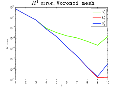
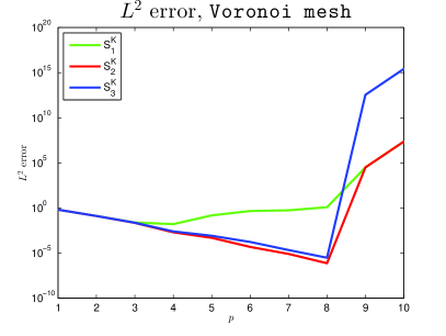
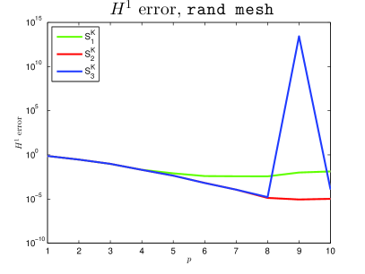
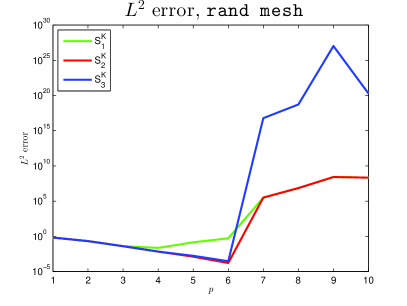
Figure 2: $p$ version of VEM. Exact solution $u_{1}$. Stabilizations employed: $S^{K}_{1}$, $S^{K}_{2}$ and $S^{K}_{3}$. Face/bulk moments employed: “standard choice”. Up-left: $H^{1}$ error on a Voronoi mesh. Up-right: $L^{2}$ error on a Voronoi mesh. Down-left: $H^{1}$ error on a rand mesh. Down-right: $L^{2}$ error on a rand mesh.

What we observe is that with no doubts the best performances are those related to stabilization $S^{K}_{2}$. The standard stabilization leads to suboptimal convergence even for moderately low degrees of accuracy; nonetheless, it prevents the error slopes to suddenly blow up as it happens for stabilization $S^{K}_{3}$. Having said this, in the forthcoming sections, we present a number of numerical tests dropping stabilization $S^{K}_{3}$.

Summary:

in $p$ VEM, employ stabilization $S^{K}_{2}$, avoid stabilizations $S^{K}_{3}$; better to avoid $S^{K}_{1}$.

3.3 Numerical results: the effects of the face/bulk moments

This section is devoted to understand the impact that the choice of face (13) and bulk (14) moments has on the convergence of the $p$ version of VEM.

We assume to use stabilizations $S^{K}_{1}$ and $S^{K}_{2}$ and we compare the effects on the performances of the method employing the “standard”, “orthogonal” and “hybrid choices”.

We begin by applying the method on the model problem with exact solution $u_{1}$ and by employing a cube mesh in Figure 3, a Voronoi mesh in Figure 4 and a rand mesh in Figure 5. We check both the $H^{1}$ and the $L^{2}$ errors.

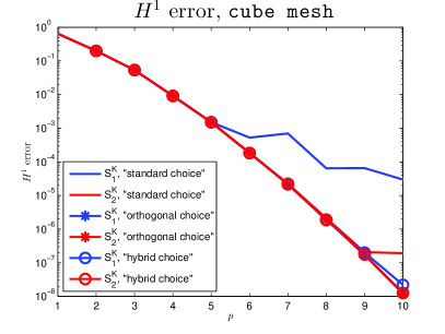
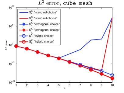
Figure 3: $p$ version of VEM. Exact solution $u_{1}$. Stabilizations employed: $S^{K}_{1}$ and $S^{K}_{2}$. Face/bulk moments employed: “standard choice”, “orthogonal choice” and “hybrid choice”. Cube mesh. Left: $H^{1}$ error. Right: $L^{2}$ error.

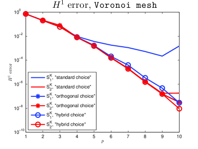
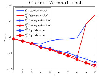
Figure 4: $p$ version of VEM. Exact solution $u_{1}$. Stabilizations employed: $S^{K}_{1}$ and $S^{K}_{2}$. Face/bulk moments employed: “standard choice”, “orthogonal choice” and “hybrid choice”. Voronoi mesh. Left: $H^{1}$ error. Right: $L^{2}$ error.

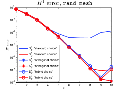
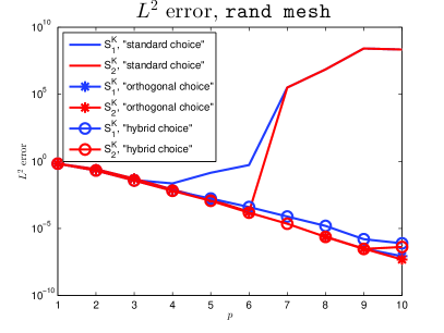
Figure 5: $p$ version of VEM. Exact solution $u_{1}$. Stabilizations employed: $S^{K}_{1}$ and $S^{K}_{2}$. Face/bulk moments employed: “standard choice”, “orthogonal choice” and “hybrid choice”. Rand mesh. Left: $H^{1}$ error. Right: $L^{2}$ error.

What we observe in Figures 3, 4 and 5 is that when employing a very regular mesh (cube mesh) the “standard choice” suffers a lack of convergence even employing stabilization $S^{K}_{2}$, which is the most robust among those we presented; on the other hand, by employing both the “orthogonal choice” and the “hybrid choice”, the method converges without any loss. Analogous comments hold true when employing a Voronoi mesh, which is less regular than the cube one, although it seems that the $H^{1}$ and $L^{2}$ errors on the Voronoi mesh employing the “orthogonal choice” and stabilization $S^{K}_{2}$ starts to grow for $p=10$.

Interestingly, analogous results are valid also when employing a much less regular mesh (with small faces, small edges) such as the rand mesh. The error slopes when employing the “orthogonal choice” and the “hybrid choice” are identical in practice up to $p=9$; for $p=10$, the “orthogonal choice” performs slightly better.

At the end of the day, we can say that in the $p$ version of VEM the “orthogonal” and the “hybrid choices” are comparable and show extremely satisfactory results.

At this point, we wonder the reasons for which the “standard choice” leads to suboptimal convergence. As discussed in Section 3.1, one possible reason is the choice of the stabilization along with its effect on the pollution factor $\alpha(p)$ defined in (26); another one is the condition number of the stiffness matrix.

As already observed, in order to see if the condition number is the reason for the suboptimal convergence, we have to test the method on a polynomial solution; for this reason, we consider in Figures 6, 7 and 8 the same set of numerical tests exhibited in Figures 3, 4 and 5 applied now to the patch test solution $u_{2}$.

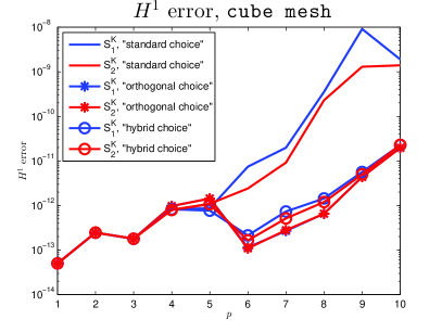
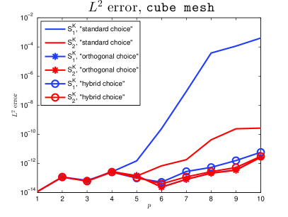
Figure 6: $p$ version of VEM. Exact solution $u_{2}$. Stabilizations employed: $S^{K}_{1}$ and $S^{K}_{2}$. Face/bulk moments employed: “standard choice”, “orthogonal choice” and “hybrid choice”. Cube mesh. Left: $H^{1}$ error. Right: $L^{2}$ error.

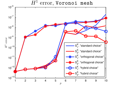
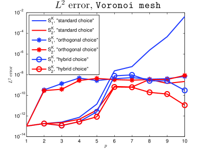
Figure 7: $p$ version of VEM. Exact solution $u_{2}$. Stabilizations employed: $S^{K}_{1}$ and $S^{K}_{2}$. Face/bulk moments employed: “standard choice”, “orthogonal choice” and “hybrid choice”. Voronoi mesh. Left: $H^{1}$ error. Right: $L^{2}$ error.

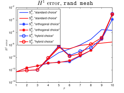
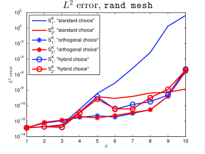
Figure 8: $p$ version of VEM. Exact solution $u_{2}$. Stabilizations employed: $S^{K}_{1}$ and $S^{K}_{2}$. Face/bulk moments employed: “standard choice”, “orthogonal choice” and “hybrid choice”. Rand mesh. Left: $H^{1}$ error. Right: $L^{2}$ error.

We deduce that the problem of unexpected decay of the error when employing the “standard choice” is not only ill-conditioning. Let us focus for instance on the Voronoi mesh. Employing the “standard choice” on the patch test, the $L^{2}$ error with $p=10$ is around $10^{-8}$ when using stabilization $S^{K}_{2}$ and around $10^{-2}$ when using stabilization $S^{K}_{1}$, while, when testing analytic solution $u_{1}$, the $L^{2}$ error with both stabilization is $10^{7}$!

Such mismatch between results approximating solutions $u_{1}$ and $u_{2}$ are not observed with the “orthogonal” and “hybrid choice”. As a consequence, the two novel choices, i.e. the “orthogonal” and the “hybrid choice”, make the method even more robust when defining the stabilization.

Summary:

in $p$ VEM, employ the “orthogonal” and the “hybrid choices” (robustness in the choice of stabilizations!); avoid the “standard choice”.

3.4 Numerical results: collapsing elements

Having observed in Section 3.3 that the “orthogonal” and the “hybrid choices” entail more robustness with respect to the choice of the stabilization than the “standard choice”, at least in the $p$ version of the method, we want to show here that such two choices perform better also when considering meshes with “collapsing polyhedra”.

For the purpose, we consider a sequence of meshes as that depicted in Figure 9. Such meshes are obtained by splitting the unit cube $[0,\,1]^{3}$ into four “boundary” polyhedra and an internal octahedron. The sequence is built by shifting two vertices of the octahedron towards $\mathbf{x}_{\Omega}=(0.5,\,0.5,\,0.5)$, the center of mass of the cube, for example we shift the points $A$ and $B$ represented in Figure 9 towards $\mathbf{x}_{\Omega}$. In this way, the volume of the octahedron collapses.

More precisely, we consider a sequence of five meshes. The first one is built by taking points $A$ and $B$ having the following coordinates:

$$A=(0.25,\,0.5,\,0.5),\quad\quad B=(0.75,\,0.5,\,0.5).$$

The other meshes are obtained by moving these two points towards $\mathbf{x}_{\Omega}$ by halving at each step their distance.

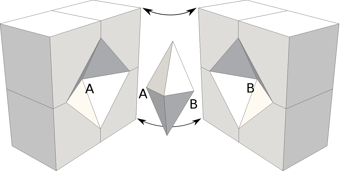
Figure 9: The mesh considered for the “collapsing test”. We highlight the points $A$ and $B$ that we shift towards the center of mass of the cube, in order to build the sequence of meshes under considerations.

We numerically investigate in Figure 10 what happens to the $H^{1}$ and the $L^{2}$ errors defined in (34), when considering as an exact solution $u_{1}$ defined in (35a) and employing stabilization $S^{K}_{2}$ defined in (28). We consider various degrees of accuracy, namely $p=3,4,5$.

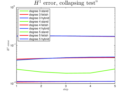
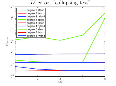
Figure 10: VEM applied to “collapsing sequences” of meshes, see Figure (9). Exact solution $u_{1}$. Stabilization employed: $S^{K}_{1}$. Face/bulk moments employed: “standard choice”, “orthogonal choice” and “hybrid choice”. Degrees of accuracy: $p=3$, $4$, $5$. Left: $H^{1}$ error. Right: $L^{2}$ error.

What we observe here is that again the “standard choice” suffers after some “collapsing iterations”.

Importantly, we carried out numerical experiments with stabilization $S^{K}_{1}$ and even worse performances of the “standard choice” have been observed.

Summary:

in VEM on meshes with “collapsing polyhedra”, employ the “orthogonal” and the “hybrid choices”; avoid the “standard choice”.

3.5 Numerical results: the $h$ version of 3D VEM

In the foregoing sections, we observed that the “orthogonal” and the ‘hybrid choice” produce similar results when dealing with the $p$ version of VEM as well as when considering meshes characterized by elements with collapsing bulk.

In this section, we consider instead the $h$ version of VEM and we compare the effects on the convergence of the error employing again the “standard”, the “orthogonal” and the “hybrid choices”.

We aim to approximate the analytic solution $u_{1}$. We consider two sequences of meshes, namely a cube mesh and Voronoi mesh, and we fix $S^{K}_{2}$ as a stabilization.

In Figures 11, 12 and 13 we perform the tests on the sequence of cube meshes whereas, in Figures 14, 15 and 16 we perform the tests on the sequence of Voronoi meshes.

Figure 11: $h$ version of VEM. Exact solution $u_{1}$. Stabilization employed: $S^{K}_{2}$. Face/bulk moments employed: “standard choice”. Cube mesh. Left: $H^{1}$ error. Right: $L^{2}$ error.

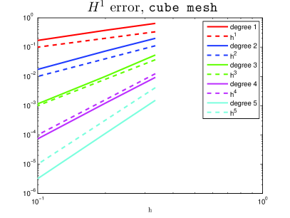
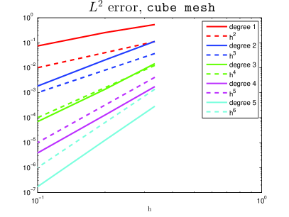
Figure 12: $h$ version of VEM. Exact solution $u_{1}$. Stabilization employed: $S^{K}_{2}$. Face/bulk moments employed: “orthogonal choice”. Cube mesh. Left: $H^{1}$ error. Right: $L^{2}$ error.

Figure 13: $h$ version of VEM. Exact solution $u_{1}$. Stabilization employed: $S^{K}_{2}$. Face/bulk moments employed: “hybrid choice”. Cube mesh. Left: $H^{1}$ error. Right: $L^{2}$ error.

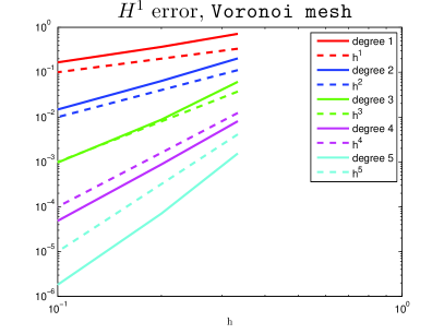
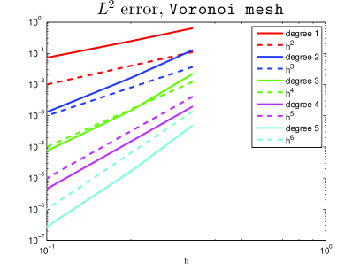
Figure 14: $h$ version of VEM. Exact solution $u_{1}$. Stabilization employed: $S^{K}_{2}$. Face/bulk moments employed: “standard choice”. Voronoi mesh. Left: $H^{1}$ error. Up-right: $L^{2}$ error.

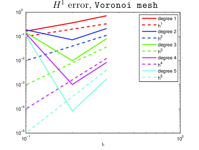
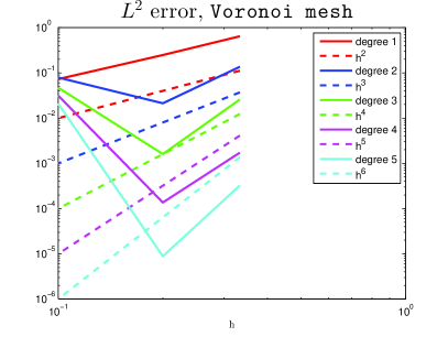
Figure 15: $h$ version of VEM. Exact solution $u_{1}$. Stabilization employed: $S^{K}_{2}$. Face/bulk moments employed: “orthogonal choice”. Voronoi mesh. Left: $H^{1}$ error. Up-right: $L^{2}$ error.

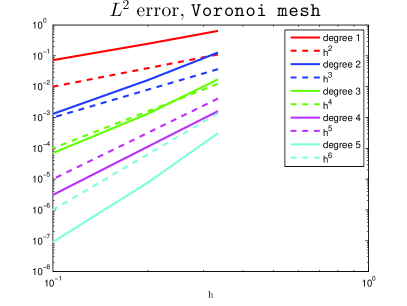
Figure 16: $h$ version of VEM. Exact solution $u_{1}$. Stabilization employed: $S^{K}_{2}$. Face/bulk moments employed: “hybrid choice”. Voronoi mesh. Left: $H^{1}$ error. Up-right: $L^{2}$ error.

What we deduce is that on sequences of regular polygons all the bases perform rather well; on the other hand, on sequences of less regular meshes, e.g. Voronoi meshes, the orthogonalization process on faces leads to very bad (even increasing sometimes) error slopes.

The reason for this bad behaviour is entirely ascribable to ill-conditioning. Indeed, in Figure 17, we apply as an example the VEM to the patch test $u_{2}$, taking for instance the Voronoi mesh and the “orthogonal choice”.

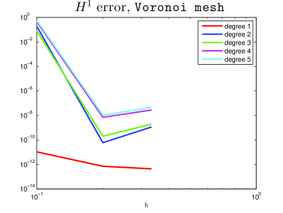
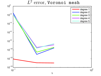
Figure 17: $h$ version of VEM. Exact solution $u_{2}$. Stabilizations employed: $S^{K}_{2}$. Face/bulk moments employed: “orthogonal choice”. Left: $H^{1}$ error “orthogonal choice”. Right: $L^{2}$ error “orthogonal choice”.

What we observe is that the error grows precisely as it grows when approximating the analytic solution in Figure 15.

Summary:

in $h$ VEM, employ “standard” and “hybrid choices”; avoid “orthogonal choice”.

4 Conclusions

In this paper, we presented numerical tests dealing with high-order Virtual Element Method for the approximation of a three dimensional Poisson problem, extending thus the numerical analysis of [11, 19].

Moreover, we tested the method employing three different stabilizations and three different choices of face/bulk degrees of freedom.

It turned out that the stabilization leading to more performing results is $S^{K}_{2}$, which has the merit of “leveling” the contribution of the consistency and stability terms in the local splitting (21).

Regarding the definition of face/bulk degrees of freedom, we have numerical evidence that the “standard choice”, i.e. moments taken with respect to (scaled and centered) monomials, leads to satisfactory decay of the errors in the $h$ version of the method, but implies suboptimal/wrong numerical results when employing both (moderately) high order degrees of accuracy and when employing meshes with “bad-shaped” elements; this suboptimality can be alleviated by considering either the “orthogonal choice” or the “hybrid choice”.

However, the “orthogonal choice” leads, on some sequences of meshes (characterized by small faces, small edges…), to inappropriate error convergence curves when employing the $h$ version of the method, whereas the “hybrid choice” seems to be more robust with this respect.

For this reason, if we have to suggest one recipe for building a VEM in three dimensions, we recommend the following:

• employ stabilization $S^{K}_{2}$;

• employ the “standard” and the “hybrid choices” for the $h$ version of the method, giving a preference to the “hybrid choice” in presence of “ collapsing” elements;

• employ the “orthogonal” and the “hybrid choices” for the $p$ version of the method.

Importantly, we also discussed the possible reasons for which the method could return in some occurrences the wrong error convergence slopes.

The first one is the condition number of the stiffness matrix, whose effect can be determined by checking the errors on the patch test, e.g. on function $u_{2}$.

The second one is the choice of the stabilization, which influences the condition number, but plays also a role in approximation estimates through the pollution factor $\alpha(p)$ defined in (26).

Appendix A A hitchhiker’s guide for the “orthogonal” and the “hybrid choice”

This appendix is devoted to discuss some implementation details of the local VEM stiffness matrix by employing specific polynomial bases introduced in Section 2.3 in the face (13) and bulk (14) moments.

Since the “standard choice” has already been investigated in [8], we split this appendix into two parts: in Appendix A.1, we discuss the details when employing the “orthogonal choice” whereas, in Appendix A.2, we discuss the details when employing the “hybrid choice”.

Henceforth we fix some notations; given $K$ polyhedron in $\mathcal{T}_{n}$, we set $N_{dof}$ the dimension of $V_{p}(K)$ and, given $F$ a face of $K$, we set $N_{dof}^{F}$ the dimension of $V_{p}(F)$; moreover, by $N_{S}$, $N_{F}$ and $N_{B}$ we denote the number of skeletal, face and bulk dofs in local space $V_{p}(K)$ defined in (16), respectively. In Section 2.3, we defined polynomial basis up to order $p-2$. In this appendix, we employ polynomials up to order $p$. In particular, we write $\{m_{\alpha}^{F}\}_{\alpha=1}^{n_{p}^{F}}$ and $\{m_{\alpha}\}_{\alpha=1}^{n_{p}}$ to denote the monomials of degree $p$ on face $F$ and in polyhedron $K$, while we write $\{\overline{m}_{\alpha}^{F}\}_{\alpha=1}^{n_{p}^{F}}$ and $\{\overline{m}_{\alpha}\}_{\alpha=1}^{n_{p}}$ to denote the $L^{2}$ orthonormal polynomials on face $F$ and in polyhedron $K$ obtained from $\{m_{\alpha}^{F}\}_{\alpha=1}^{n_{p}^{F}}$ and $\{m_{\alpha}\}_{\alpha=1}^{n_{p}}$ via a stable Gram-Schmidt process, respectively.

When dealing with calculations between vectors-matrices, we employ the following notation:

$$\mathbf{A}(i:j,l:k)\quad\quad\quad\forall\,\mathbf{A}\in\mathbb{R}^{n,m},$$

is the submatrix of $\mathbf{A}$ from row $i$ to $j$ and from column $\ell$ to column $k$. If no indications concerning rows-columns are given, then it means that we are considering the full matrix.

We extensively make usage of the two natural bijections (30) and (31).

The construction of the local stiffness matrix in the “standard case” is based on the following matrices, whose implementation has been already discussed in [8], both in polyhedron $K$:

$$\mathbf{G}_{\alpha,\beta}=\begin{cases}\begin{cases}\sum_{i=1}^{N_{V}}(m_{\beta}(\nu_{i}))&\text{if }p=1\\ \int_{K}m_{\beta}&\text{otherwise}\\ \end{cases}&\text{if }\alpha=1\\ (\nabla m_{\alpha},\nabla m_{\beta})_{0,K}&\text{otherwise}\\ \end{cases},$$ (36)

$$\widetilde{\mathbf{G}}_{\alpha,\beta}=(\nabla m_{\alpha},\nabla m_{\beta})_{0,K},\quad\mathbf{B}_{\alpha,i}=\begin{cases}P_{0}\varphi_{i}&\text{if }\alpha=1\\ (\nabla m_{\alpha},\nabla\varphi_{i})_{0,K}&\text{otherwise}\\ \end{cases},$$

$$\mathbf{D}_{i,\alpha}=\text{dof}_{i}(m_{\alpha}),\quad\mathbf{H}_{\alpha,\beta}=(m_{\alpha},m_{\beta})_{0,K},\quad\mathbf{C}_{\alpha,i}=(m_{\alpha},\varphi_{i})_{0,K},$$

for all $\alpha$, $\beta=1,\dots,n_{p}$ and for all $i=1,\dots,N_{dof}$, where we recall that $N_{V}$ and $\{\nu_{i}\}_{i=1}^{N_{V}}$ are the number and the set of vertices of $K$, both on face $F$:

$$\mathbf{G}^{F}_{\alpha,\beta}=\begin{cases}\begin{cases}\sum_{i=1}^{N_{V}^{F}}(m_{\beta}^{F}(\nu_{i}^{F}))&\text{if }p=1\\ \int_{K}m_{\beta}^{F}&\text{otherwise}\\ \end{cases}&\text{if }\alpha=1\\ (\nabla m_{\alpha}^{F},\nabla m_{\beta}^{F})_{0,F}&\text{otherwise}\\ \end{cases},$$ (37)

$$\widetilde{\mathbf{G}}^{F}_{\alpha,\beta}=(\nabla m_{\alpha}^{F},\nabla m_{\beta}^{F})_{0,K},\quad\mathbf{B}_{\alpha,i}=\begin{cases}P_{0}\varphi_{i}&\text{if }\alpha=1\\ (\nabla m_{\alpha}^{F},\nabla\varphi_{i})_{0,F}&\text{otherwise}\\ \end{cases},$$

$$\mathbf{D}_{i,\alpha}=\text{dof}_{i}(m_{\alpha}^{F}),\quad\mathbf{H}_{\alpha,\beta}=(m_{\alpha}^{F},m_{\beta}^{F})_{0,K},\quad\mathbf{C}_{\alpha,i}=(m_{\alpha}^{F},\varphi_{i})_{0,F},$$

for all $\alpha$, $\beta=1,\dots,n_{p}^{F}$ and for all $i=1,\dots,N_{dof}^{F}$, where we recall that $N_{V}^{F}$ and $\{\nu_{i}^{F}\}_{i=1}^{N_{V}^{F}}$ are the number and the set of vertices of $F$.

In the two forthcoming appendices, we explain how to construct the counterparts of the matrices defined in (36) and (37) with the “orthogonal” and the “hybrid choices”. Since with these two choices we employ $L^{2}$ orthonormal polynomial bases, we also need the (lower triangular) matrices containing the orthonormalizing coefficients with respect to the monomial bases of $\mathbb{P}_{p}(K)$ and $\mathbb{P}_{p}(F)$, respectively. Such matrices are denoted by $\mathbf{GS}$, matrix belonging to $\mathbb{R}^{n_{p}\times n_{p}}$ (on polyhedron $K$), and $\mathbf{GS}^{F}$, matrix belonging to $\mathbb{R}^{n_{p}^{F}\times n_{p}^{F}}$ (on face $F$).

In the remainder of this appendix, we denote the local VEM matrices, the local degrees of freedom and the local canonical basis functions with a bar at the top of each of them.

A.1 A hitchhiker’s guide for the “orthogonal choice”

The aim of the present appendix, is to give some details for what concerns the computation of the counterpart of the matrices in (36) employing the face/bulk polynomial bases of the so-called “orthogonal choice” discussed in Section 2.3. In particular, we fix bases made of $L^{2}$ orthonormal polynomials both on faces and in the bulk.

The assembling of the local stiffness matrix boils down to the construction in [8] and depends on the choice of the local stabilization, see Section 2.2.

A.1.1 Matrices $\overline{\mathbf{G}}$ and $\overline{\widetilde{\mathbf{G}}}$

We start with matrix $\overline{\widetilde{\mathbf{G}}}$ which is defined as:

$$\overline{\widetilde{\mathbf{G}}}=(\nabla\overline{m}_{\alpha},\nabla\overline{m}_{\beta})_{0,K}\quad\forall\,\alpha,\,\beta=1,\dots,n_{p}.$$

One simply has:

$$\overline{\widetilde{\mathbf{G}}}=\mathbf{GS}\cdot\widetilde{\mathbf{G}}\cdot\mathbf{GS}^{T}.$$

Next, we consider matrix $\overline{\mathbf{G}}$ defined as:

$$\overline{\widetilde{\mathbf{G}}}_{\boldsymbol{\alpha},\boldsymbol{\beta}}=\begin{cases}P_{0}(\overline{m}_{\beta})&\text{if }\alpha=1\\ (\nabla\overline{m}_{\alpha},\nabla\overline{m}_{\beta})_{0,K}&\text{otherwise}\end{cases}\quad\forall\,\alpha,\,\beta=1,\dots,n_{p},$$

where, recalling that $\{\nu_{i}\}_{i=1}^{N_{V}}$ is the set of vertices of $K$:

$$P_{0}(\cdot)=\begin{cases}\frac{1}{N_{V}}\sum_{i=1}^{N_{V}}\cdot(\nu_{i})&\text{if }p=1\\ \frac{1}{|K|}\int_{K}\cdot&\text{otherwise}\\ \end{cases}.$$

Clearly, we only have to treat the case $\alpha=1$. We distinguish two cases.

If $p=1$, then we have:

$$P_{0}(\overline{m}_{\beta})=\frac{1}{N_{V}}\overline{m}_{\beta}(\nu_{i})\quad\forall\,\beta=1,\dots,n_{p}$$

and therefore

$$P_{0}(\overline{m}_{\beta}) =\frac{1}{N_{V}}\sum_{i=1}^{N_{V}}\left(\sum_{\gamma\leq\beta}\mathbf{GS}_{\beta,\gamma}m_{\gamma}(\nu_{i})\right)=\sum_{\gamma\leq\beta}\mathbf{GS}_{\beta,\gamma}\left(\frac{1}{N_{V}}\sum_{i=1}^{N_{V}}m_{\gamma}(\nu_{i})\right)$$

$$=\sum_{\gamma\leq\beta}\mathbf{GS}_{\beta,\gamma}\mathbf{G}_{1,\gamma}=\mathbf{GS}(\beta,1:\beta)\cdot\mathbf{G}(1,1:\beta)^{T}\quad\forall\,\beta=1,\dots,n_{p}.$$

If, on the other hand, $p\geq 2$:

$$P_{0}(\overline{m}_{\beta}) =\frac{1}{|K|}\int_{K}\overline{m}_{\beta}=\mathbf{GS}_{1,1}^{-1}\frac{1}{|K|}\int_{K}\overline{m}_{\beta}\mathbf{GS}_{1,1}$$

$$=\mathbf{GS}_{1,1}^{-1}\frac{1}{|K|}\int_{K}\overline{m}_{1}\overline{m}_{\beta}=\begin{cases}\frac{1}{\mathbf{GS}_{1,1}|K|}&\text{if }\beta=1\\ 0&\text{else}\\ \end{cases}\quad\forall\,\beta=1,\dots,n_{p},$$

since basis $\{\overline{m}_{\alpha}\}_{\alpha=1}^{n_{p}}$ is $L^{2}(K)$ orthonormal by construction.

A.1.2 Matrix $\overline{\mathbf{D}}$

We define matrix $\overline{\mathbf{D}}$ as:

$$\overline{\mathbf{D}}_{i,\alpha}=\overline{\text{dof}}_{i}(\overline{m}_{\alpha})\quad\forall\,i=1,\dots,N_{dof},\,\forall\,\alpha=1,\dots,n_{p}.$$

Let us consider firstly the boundary dofs. For all $i=1,\dots,N_{S}$ and for all $\alpha=1,\dots,n_{p}$:

$$\overline{\mathbf{D}}_{i,\alpha}=\overline{\text{dof}}_{i}(\overline{m}_{\alpha})=\overline{m}_{\alpha}(\xi_{i})=\sum_{\beta\leq\alpha}\mathbf{GS}_{\alpha,\beta}\,m_{\beta}(\xi_{i})=\sum_{\beta\leq\alpha}\mathbf{GS}_{\alpha,\beta}\mathbf{D}_{i,\beta}=\mathbf{D}(i,1:\alpha)^{T}\cdot\mathbf{GS}(\alpha,1:\alpha)^{T},$$

where $\xi_{i}$ is a proper node on the boundary. In short:

$$\overline{\mathbf{D}}(1:N_{S},1:n_{p})=\mathbf{D}(1:N_{S},1:n_{p})\cdot\mathbf{GS}^{T}.$$

Next, we deal with the face dofs. Assume that the $i$-th $\overline{\text{dof}}$ is associated with polynomial $\overline{m}_{\gamma}^{F}$. Then, for all $i=N_{S}+1,\dots,N_{S}+N_{F}$ and for all $\alpha=1,\dots,n_{p}$:

$$\overline{\text{dof}}_{i}(\overline{m}_{\alpha})=\frac{1}{|F|}\int_{F}\overline{m}_{\gamma}^{F}\overline{m}_{\alpha}=\sum_{\beta\leq\alpha}\mathbf{GS}_{\alpha,\beta}\frac{1}{|F|}\int_{F}\overline{m}_{\gamma}^{F}m_{\beta}=\sum_{\beta\leq\alpha}\mathbf{GS}_{\alpha,\beta}\left\{\sum_{\delta\leq\gamma}\mathbf{GS}_{\gamma,\delta}^{F}\frac{1}{|F|}\int_{F}m_{\delta}^{F}m_{\beta}\right\}.$$

In short:

$$\overline{\mathbf{D}}(N_{S}+1:N_{S}+N_{F}+1,1:n_{p})=\mathbf{GS}^{F}(1:n_{p-2}^{F},1:n_{p-2}^{F})\cdot\mathbf{D}(N_{S}+1:N_{S}+N_{F}+1,1:n_{p-2})\cdot\mathbf{GS}^{T}.$$

Finally, we treat the bulk dofs. Assume that the $i$-th dof is associated with polynomial $\overline{m}_{\gamma}$. Then, for all $i=N_{S}+N_{F}+1,\dots,N_{S}+N_{F}+N_{B}$ and for all $\alpha=1,\dots,n_{p}$:

$$\overline{\text{dof}}_{i}(\overline{m}_{\alpha})=\frac{1}{|K|}\int_{K}\overline{m}_{\alpha}\overline{m}_{\gamma}=\frac{1}{|K|}\delta_{\alpha,i}.$$

A.1.3 Matrix $\overline{\mathbf{H}}$

We define matrix $\overline{\mathbf{H}}$ as:

$$\overline{\mathbf{H}}_{\alpha,\beta}=(\overline{m}_{\alpha},\overline{m}_{\beta})_{0,K}\quad\forall\,\alpha,\,\beta=1,\dots,n_{p}.$$

One directly has:

$$\overline{\mathbf{H}}=\mathbf{GS}\cdot\mathbf{H}\cdot\mathbf{GS}^{T}=\textbf{Id}.$$

As a byproduct, we observe that by verifying this last equality one can check whether $\mathbf{GS}$ has been actually properly computed.

A.1.4 Matrix $\overline{\mathbf{B}}$

We define matrix $\overline{\mathbf{B}}$ as follows:

$$\overline{\mathbf{B}}_{\alpha,i}=\begin{cases}P_{0}(\overline{\varphi}_{i})&\text{if }\alpha=1\\ (\nabla\overline{m}_{\alpha},\nabla\overline{\varphi}_{i})_{0,K}&\text{otherwise}\\ \end{cases}\quad\forall\,\alpha=1,\dots,n_{p},\,\forall\,i=1,\dots,N_{dof}.$$

We firstly deal with the first line and we consider the two cases $p=1$ and $p\geq 2$.

• $P_{0}(\overline{\varphi}_{i})=\frac{1}{N_{V}}\sum_{i=1}^{N_{V}}\overline{\varphi}_{i}(\nu_{i})$. Thus, $\overline{\mathbf{B}}_{1,i}=\mathbf{B}_{1,i}$ for all $i=1,\dots,N_{dof}$, since the elements of the new basis coincide with the old ones on the skeleton of the mesh.

• In this case:

  $$P_{0}(\overline{\varphi}_{i})= \frac{1}{|K|}\int_{K}\overline{\varphi}_{i}=\mathbf{GS}^{-1}_{1,1}\frac{1}{|K|}\int_{K}\overline{\varphi}_{i}\mathbf{GS}_{1,1}=\mathbf{GS}^{-1}_{1,1}\frac{1}{|K|}\int_{K}\overline{\varphi}_{i}\overline{m}_{1}$$

  $$=\begin{cases}\mathbf{GS}^{-1}_{1,1}&\text{if }\overline{\varphi}_{i}\text{ is the first bulk basis element}\\ 0&\text{else}\\ \end{cases}\quad\forall\,i=1,\dots,N_{dof},$$

  since $\overline{m}_{1}=\mathbf{GS}_{1,1}m_{1}=\mathbf{GS}_{1,1}$. Thus, we can copy the old line and multiply it for $\mathbf{GS}_{1,1}^{-1}$, i.e. $\overline{\mathbf{B}}_{1,i}=\mathbf{GS}_{1,1}^{-1}\mathbf{B}_{1,i}$.

Next, we treat the remaining lines. We must compute $(\nabla\overline{m}_{\alpha},\nabla\overline{\varphi}_{i})_{0,K}$. We consider three different situations.

• We assume $\overline{\varphi}_{i}$ edge basis element. Then:

  $$(\nabla\overline{m}_{\alpha},\nabla\overline{\varphi}_{i})_{0,K}=(-\Delta\overline{m}_{\alpha},\overline{\varphi}_{i})_{0,K}+(\partial_{\mathbf{n}}\overline{m}_{\alpha},\overline{\varphi}_{i})_{0,\partial K}$$

  $$=\sum_{F\in\partial K}(\partial_{\mathbf{n}}\overline{m}_{\alpha},\overline{\varphi}_{i})_{0,F}\quad\forall\,\alpha=1,\dots,n_{p},\,\forall\,i=1,\dots,N_{S}.$$

  Therefore, it suffices to compute integrals over faces. For the purpose, we decompose $\partial_{\mathbf{n}}\overline{m}_{\alpha}$ on each face $F$ as a linear combination of elements in the $L^{2}(F)$ orthonormal basis $\{\overline{m}_{\beta}^{F}\}_{|\boldsymbol{\beta}|=0}^{p-1}$:

  $$\partial_{\mathbf{n}}\overline{m}_{\alpha}|_{F}=\sum_{|\boldsymbol{\beta}|=0}^{p-1}\overline{\lambda}_{\alpha,\beta}^{F}\overline{m}_{\beta}^{F}\quad\quad\forall\,F\in\partial K,\quad\forall\,\alpha=1,\dots,n_{p}.$$ (38)

  In order to be able to compute the coefficients $\overline{\lambda}_{\alpha,\beta}^{F}$, we test (38) with $\overline{m}_{\gamma}^{F}$ with $\gamma=1,\dots,n_{p-1}$ and get by orthonormality:

  $$\overline{\lambda}_{\alpha,\mathbf{n}}^{F}=(\partial_{\mathbf{n}}\overline{m}_{\alpha},\overline{m}_{\gamma}^{F})_{0,F} =\sum_{\beta\leq\alpha}\mathbf{GS}_{\alpha,\beta}\left\{\sum_{\delta\leq\gamma}\mathbf{GS}_{\gamma,\delta}^{F}(\partial_{\mathbf{n}}m_{\beta},m_{\delta}^{F})_{0,F}\right\}$$ (39)

  $$\quad\forall\,\alpha=1,\dots,n_{p},\,\forall\,\gamma=1,\dots,n_{p-1},$$

  which is easily computable:

  $$\overline{\lambda}_{\alpha,\gamma}^{F}=\mathbf{GS}(\alpha,1:n_{p})\cdot\boldsymbol{\Lambda}^{F}\cdot\mathbf{GS}^{F}(\gamma,1:n_{p-1}^{F})^{T}\quad\forall\,\alpha=1,\dots,n_{p},\,\forall\,\gamma=1,\dots,n_{p-1},$$

  where:

  $$\boldsymbol{\Lambda}^{F}_{\beta,\delta}=(\partial_{\mathbf{n}}m_{\beta},m_{\delta}^{F})_{0,F}\quad\quad\forall\,\beta=1,\dots,n_{p},\,\forall\,\delta=1,\dots,n_{p-1}$$

  is computable by a simple integration of $L^{2}$ products on monomials.

  In short, if we call $\boldsymbol{\overline{\mathbf{\Lambda}}}^{F}$ the matrix of the coefficients of expansion (38) on face $F$, then we have:

  $$\boldsymbol{\overline{\mathbf{\Lambda}}}^{F}=\mathbf{GS}\cdot\boldsymbol{\Lambda}^{F}\cdot\mathbf{GS}^{F}(1:n_{p-1}^{F},1:n_{p-1}^{F})^{T}.$$

  As a consequence, on each face $F$, we get by using the definition of the enhancing constraints:

  $$(\partial_{\mathbf{n}}\overline{m}_{\alpha},\overline{\varphi}_{i})_{0,F} =\sum_{|\boldsymbol{\beta}|=0}^{p-1}\overline{\lambda}_{\alpha,\beta}^{F}(\overline{m}_{\beta}^{F},\overline{\varphi}_{i})_{0,F}=\sum_{|\boldsymbol{\beta}|=p-1}\overline{\lambda}_{\alpha,\beta}^{F}(\overline{m}_{\beta}^{F},\overline{\varphi}_{i})_{0,F}$$ (40)

  $$=\sum_{|\boldsymbol{\beta}|=p-1}\overline{\lambda}_{\alpha,\beta}^{F}(\overline{m}_{\beta}^{F},\overline{\Pi}^{\nabla,F}_{p}\overline{\varphi}_{i})_{0,F}\quad\forall\,\alpha=1,\dots,n_{p},\,\forall i=N_{S}+1,\dots,N_{S}+N_{F},$$

  where $\overline{\Pi}^{\nabla,F}_{p}$ denotes the $H^{1}$ projection on the polynomial space spanned by the $L^{2}(F)$ orthonormal basis $\{\overline{m}_{\alpha}^{F}\}_{\alpha=1}^{n_{p}^{F}}$, which can be computed on face $F$ following [19]. The quantity in (40) can be computed; in fact:

  $$\sum_{|\boldsymbol{\beta}|=p-1}\overline{\lambda}_{\alpha,\beta}^{F}(\overline{m}_{\beta}^{F},\overline{\Pi}^{\nabla,F}_{p}\overline{\varphi}_{i})_{0,F}=\sum_{|\boldsymbol{\beta}|=p-1}\overline{\lambda}_{\alpha,\beta}^{F}\left(\overline{m}_{\beta}^{F},\sum_{|\boldsymbol{\gamma}|=0}^{p}\overline{\chi}_{\gamma,i}^{F}\overline{m}_{\gamma}^{F}\right)_{0,F}=\sum_{|\boldsymbol{\beta}|=p-1}\overline{\lambda}_{\alpha,\beta}^{F}\overline{\chi}_{\beta,i}^{F}.$$ (41)

  In order to conclude, one sums (41) on all the faces.

• Let now $\overline{\varphi}_{i}$ be a face basis element. Then:

  $$(\nabla\overline{m}_{\alpha},\nabla\overline{\varphi}_{i})_{0,K} =(\partial_{\mathbf{n}}\overline{m}_{\alpha},\overline{\varphi}_{i})_{0,\partial K}$$ (42)

  $$=\sum_{F\in\partial K}(\partial_{\mathbf{n}}\overline{m}_{\alpha},\overline{\varphi}_{i})_{0,F}\quad\forall\,\alpha=1,\dots,n_{p},\,\forall\,i=N_{S}+1,\dots,N_{S}+N_{F}.$$

  Plugging expansion (38) into (42) and denoting by $\widetilde{F}$ the face associated with basis element $\overline{\varphi}_{i}$:

  $$(\nabla\overline{m}_{\alpha},\overline{\varphi}_{i})_{0,K}=\sum_{F\in\partial K}\sum_{|\boldsymbol{\beta}|=0}^{p-1}\lambda^{F}_{\alpha,\beta}(\overline{m}_{\beta}^{F},\overline{\varphi}_{i})_{0,F}$$

  $$=\left(\sum_{F\in\partial K}\sum_{|\boldsymbol{\beta}|=p-1}\lambda^{F}_{\alpha,\beta}(\overline{m}_{\beta}^{F},\overline{\Pi}^{\nabla,F}_{p}\overline{\varphi}_{i})_{0,F}\right)+|\widetilde{F}|\overline{\lambda}_{\alpha,i}^{\widetilde{F}}\quad\forall\,\alpha=1,\dots,n_{p},\,\forall\,i=N_{S}+1,\dots,N_{S}+N_{F},$$

  where $\overline{\lambda}^{F}_{\alpha,i}$ is computed as in (39) for all faces $F\in\partial K$ and where we are assuming that $\overline{\varphi}_{i}$ is the face element associated with $\overline{m}_{\beta}^{\widetilde{F}}$. The integrals over the faces involving $\Pi^{\nabla}_{p}$ can be computed as in (41).

• Finally, we assume that $\overline{\varphi}_{i}$ is a bulk basis element. Then:

  $$(\nabla\overline{m}_{\alpha},\nabla\overline{\varphi}_{i})_{0,K}=(-\Delta\overline{m}_{\alpha},\overline{\varphi}_{i})_{0,K}\quad\forall\,\alpha=1,\dots,n_{p},\,\forall\,i=N_{S}+N_{F}+1,\dots,N_{S}+N_{F}+N_{B}.$$ (43)

  As a consequence, we have to expand $-\Delta\overline{m}_{\alpha}$ in terms of the $L^{2}(K)$ orthonormal basis $\{\overline{m}_{\alpha}\}_{\alpha=1}^{n_{p-2}}$ as:

  $$-\Delta\overline{m}_{\alpha}=\sum_{|\boldsymbol{\beta}|=0}^{p-2}\overline{\mu}_{\alpha,\beta}\overline{m}_{\beta}\quad\forall\,\alpha=1,\dots,n_{p}.$$ (44)

  We test (44) with $\overline{m}_{\gamma}$, $|\boldsymbol{\gamma}|=0,\dots,p-1$ and get by orthonormality:

  $$\overline{\mu}_{\alpha,\beta}=(-\Delta\overline{m}_{\alpha},\overline{m}_{\gamma})_{0,K}=\overline{\mathbf{L}}_{\alpha,\gamma}\quad\forall\,\alpha=1,\dots,n_{p},\,\forall\,\beta=1,\dots,n_{p-2},$$ (45)

  which is actually computable. In fact:

  $$(-\Delta\overline{m}_{\alpha},\overline{m}_{\gamma})_{0,K}=\mathbf{GS}(\alpha,1:n_{p})\cdot\mathbf{L}\cdot\mathbf{GS}(\gamma,1:n_{p-2})^{T}\quad\forall\,\alpha=1,\dots,n_{p},\,\forall\,\gamma=1,\dots,n_{p-2},$$

  where matrix $\mathbf{L}$ can be computed as:

  $$\mathbf{L}_{\alpha,\beta}=(-\Delta m_{\alpha},m_{\gamma})_{0,K}$$

  $$=-\frac{1}{h_{K}^{2}}\left(\alpha_{1}(\alpha_{1}-1)(m_{\boldsymbol{\alpha}_{1}},m_{\gamma})_{0,K}+\alpha_{2}(\alpha_{2}-1)(m_{\boldsymbol{\alpha}_{2}},m_{\gamma})_{0,K}+\alpha_{3}(\alpha_{3}-1)(m_{\boldsymbol{\alpha}_{3}},m_{\gamma})_{0,K}\right)$$

  $$=-\frac{1}{h_{K}^{2}}\left(\alpha_{1}(\alpha_{1}-1)\mathbf{H}_{\boldsymbol{\alpha}_{1},\beta}+\alpha_{2}(\alpha_{2}-1)\mathbf{H}_{\boldsymbol{\alpha}_{2},\beta}+\alpha_{3}(\alpha_{3}-1)\mathbf{H}_{\boldsymbol{\alpha}_{3},\beta}\right)$$

  $$\forall\,\alpha=1,\dots,n_{p},\,\forall\,\beta=1,\dots,n_{p-2},$$

  having set:

  $$\boldsymbol{\alpha}_{1}=(\alpha_{1}-2,\alpha_{2},\alpha_{3}),\quad\boldsymbol{\alpha}_{2}=(\alpha_{1},\alpha_{2}-2,\alpha_{3}),\quad\boldsymbol{\alpha}_{3}=(\alpha_{1},\alpha_{2},\alpha_{3}-2).$$

  Inserting (44) and (45) in (43), we obtain:

  $$(\nabla\overline{m}_{\alpha},\nabla\overline{\varphi}_{i})_{0,K} =\sum_{|\beta|=0}^{p-2}\mu_{\alpha,\beta}(\overline{m}_{\beta},\overline{\varphi}_{i})_{0,K}$$

  $$=|K|\mu_{\alpha,i}\quad\forall\,\alpha=1,\dots,n_{p},\,\forall\,i=N_{S}+N_{F}+1,\dots,N_{S}+N_{F}+N_{B}.$$

A.1.5 Matrix $\overline{\mathbf{C}}$

We define matrix $\overline{\mathbf{C}}$ as:

$$\overline{\mathbf{C}}_{\alpha,i}=(\overline{m}_{\alpha},\overline{\varphi}_{i})_{0,K}\quad\forall\,\alpha=1,\dots,n_{p},\,\forall\,i=1,\dots,N_{dof}.$$

It is also clear that, for all $\alpha=1,\dots,n_{p-2}$ and for all $i=1,\dots,N_{dof}$:

$$(\overline{m}_{\alpha},\overline{\varphi}_{i})_{0,K}=\begin{cases}0&\text{if }\overline{\varphi}_{i}\text{ is an edge or face basis element}\\ |K|\frac{1}{|K|}\int_{K}\overline{m}_{\alpha}\overline{\varphi}_{i}=\delta_{i,\alpha}|K|&\text{otherwise}\\ \end{cases}.$$

For what concerns the other lines, one employs the so-called enhancing technique [8]. More precisely, one sets:

$$\overline{\mathbf{C}}(n_{p-2}+1:n_{p},1:N_{dof})=\left[\overline{\mathbf{G}}^{-1}\cdot\overline{\mathbf{B}}\right](n_{p-2}+1:n_{p},1:N_{dof}).$$

A.2 A hitchhiker’s guide for the “hybrid choice”

The aim of the present appendix, is to give some details for what concerns the computation of the counterpart of the matrices in (36) employing the face/bulk polynomial bases of the so-called “hybrid choice” discussed in Section 2.3. In particular, we fix bases made of $L^{2}$ orthonormal polynomials in the bulk and standard monomials on faces.

The assembling of the local stiffness matrix boils down to the construction in [8] and depends on the choice of the local stabilization, see Section 2.2.

Henceforth, we denote with a bar at the top and hyb as subscript the local VEM matrices, the local degrees of freedom and the local canonical basis functions. It is easy to check that:

$$\overline{\widetilde{\mathbf{G}}}_{hyb}=\overline{\widetilde{\mathbf{G}}},\quad\quad\overline{\mathbf{G}}_{hyb}=\overline{\mathbf{G}},\quad\quad\overline{\mathbf{H}}_{hyb}=\overline{\mathbf{H}}.$$

For what concerns matrix $\overline{\mathbf{D}}_{hyb}$ we observe that is coincides with matrix $\overline{\mathbf{D}}$, with the exception of the entries related to face dofs. In this case, one has:

$$\overline{\mathbf{D}}_{hyb}(N_{S}+1:N_{S}+N_{F},1:n_{p})=\mathbf{D}(N_{S}+1:N_{S}+N_{F},1:n_{p-2})\cdot\mathbf{GS}^{T}.$$

The treatment of matrix $\overline{\mathbf{B}}_{hyb}$ is rather different. It coincides with $\overline{\mathbf{B}}$ when considering the first line and when considering all the columns associated with bulk dofs.

Let us fix our attention to the columns associated with skeleton dofs. In this case, we have:

$$(\nabla\overline{m}_{\alpha},\nabla\overline{\varphi}_{{hyb},i})_{0,K}=\sum_{F\in\partial K}(\partial_{n}\overline{m}_{\alpha},\overline{\varphi}_{{hyb},i})\quad\forall\,\alpha=1,\dots,n_{p},\,\forall\,i=1,\dots,N_{S}.$$ (46)

We expand $\partial_{n}\overline{m}_{\alpha}$ on each face $F$ into a combination of elements $\{m_{\beta}^{F}\}_{\beta=1}^{n_{p-1}^{F}}$, which we recall is the standard (scaled and centered) monomial basis on face $F$:

$$\partial_{\mathbf{n}}\overline{m}_{\alpha}|_{F}=\sum_{\beta=1}^{n_{p-1}^{F}}\overline{\lambda}^{F}_{{hyb},\alpha,\beta}m_{\beta}^{F}\quad\forall\,F\in\partial K,\,\forall\,\alpha=1,\dots,n_{p}.$$ (47)

By testing (47) with $m_{\gamma}^{F}$, for $\gamma=1,\dots,n_{p-1}^{F}$, we write for all faces $F$:

$$\sum_{\beta=1}^{n_{p-1}^{F}}\overline{\lambda}^{F}_{{hyb},\alpha,\beta}(m_{\beta}^{F},m_{\gamma}^{F})_{0,F}=(\partial_{n}\overline{m}_{\alpha},m_{\gamma}^{F})_{0,F}.$$

Therefore, if we want to have an explicit representation of the coefficients $\overline{\lambda}^{F}_{{hyb},\alpha,\beta}=\overline{\mathbf{\Lambda}}^{F}_{hyb}$ for $\alpha=1,\dots,n_{p}$, $\beta=1,\dots,n_{p-1}^{F}$, we have to compute:

$$\overline{\mathbf{\Lambda}}^{F}_{hyb}=\overline{\mathbf{M}}^{F}_{hyb}\cdot\mathbf{H}^{F}(1:n_{p-1}^{F},1:n_{p-1}^{F})^{-1},$$

where $\mathbf{H}^{F}$ denotes the standard 2D VEM matrix on face $F$ and where:

$$(\overline{\mathbf{M}}_{hyb}^{F})_{\alpha,\gamma}=(\partial_{\mathbf{n}}\overline{m},m_{\gamma}^{F})_{0,F}\quad\forall\,\alpha=1,\dots,n_{p},\,\forall\,\gamma=1,\dots,n_{p-1}^{F},$$

which is easily computable.

Having now the coefficients $\overline{\lambda}^{F}_{{hyb},\alpha,\beta}$, we obtain from (46) and using that $\overline{\varphi}_{{hyb},i}|_{\partial K}=\varphi_{i}|_{\partial K}$ for all $i=1,\dots,N_{S}$:

$$(\partial\overline{m}_{\alpha},\nabla\overline{\varphi}_{{hyb},i})_{0,K} =\sum_{F\in\partial K}(\partial_{\mathbf{n}}\overline{m}_{\alpha},\overline{\varphi}_{{hyb},i})_{0,F}=\sum_{F\in\partial K}(\partial_{\mathbf{n}}\overline{m}_{\alpha},\varphi_{i})_{0,F}$$

$$=\sum_{F\in\partial K}\left\{\sum_{\beta=1}^{n_{p-1}^{F}}\overline{\lambda}^{F}_{{hyb},\alpha,\beta}(m_{\beta}^{F},\varphi_{i})_{0,K}\right\}=\sum_{F\in\partial K}\left\{\sum_{\beta=n_{p-2}^{F}+1}^{n_{p-1}^{F}}\overline{\lambda}^{F}_{{hyb},\alpha,\beta}(m_{\beta}^{F},\varphi_{i})_{0,K}\right\}$$

$$=\sum_{F\in\partial K}\left\{\sum_{\beta=n_{p-2}^{F}+1}^{n_{p-1}^{F}}\overline{\lambda}^{F}_{{hyb},\alpha,\beta}(m_{\beta}^{F},\Pi^{\nabla,F}_{p}\varphi_{i})_{0,K}\right\}\quad\forall\,\alpha=1,\dots,n_{p},\,\forall\,i=1,\dots,N_{S}.$$

This is equivalent to say:

$$(\overline{\mathbf{B}}_{hyb})_{\alpha,i}=\overline{\mathbf{\Lambda}}^{F}_{hyb}(1:n_{p},n_{p-2}^{F}+1:n_{p-1}^{F})\cdot\mathbf{H}^{F}(n_{p-2}^{F}+1:n_{p-1}^{F})\cdot\mathbf{\Pi^{\nabla,*,F}}(1:n_{p},1:N_{S}),$$

where $\mathbf{\Pi^{\nabla,*,F}}=\overline{\mathbf{G}}_{hyb}^{-1}\cdot\overline{\mathbf{B}}_{{hyb}}$.

The case $\overline{\varphi}_{{hyb},i}$ face basis element is dealt with in an utterly analogous way by noting that:

$$(\nabla\overline{m}_{\alpha},\nabla\overline{\varphi}_{{hyb},i})_{0,K}=\sum_{\beta=n_{p-2}^{\widetilde{F}}+1}^{n_{p-1}^{\widetilde{F}}}\overline{\lambda}^{\widetilde{F}}_{{hyb},\alpha,\beta}(m_{\beta}^{\widetilde{F}},\Pi^{\nabla,\widetilde{F}}\varphi_{i})_{0,\widetilde{F}}+|\widetilde{F}|,$$

where $\widetilde{F}$ is the face associated with $\overline{\varphi}^{F}_{{hyb},i}$.

References

- [1] B. Ahmad, A. Alsaedi, F. Brezzi, L.D. Marini, and A. Russo. Equivalent projectors for Virtual Element Method. Comput. Math. Appl., 66(3):376–391, 2013.
- [2] P. F. Antonietti, L. Mascotto, and M. Verani. A multigrid algorithm for the -version of the Virtual Element Method. https://arxiv.org/abs/1703.02285, 2017.
- [3] F. Bassi, L. Botti, A. Colombo, D. A. Di Pietro, and P. Tesini. On the flexibility of agglomeration based physical space discontinuous Galerkin discretizations. J. Comput. Phys., 231(1):45–65, 2012.
- [4] L. Beirão da Veiga, F. Brezzi, A. Cangiani, G. Manzini, L.D. Marini, and A. Russo. Basic principles of Virtual Element Methods. Math. Models Methods Appl. Sci., 23(01):199–214, 2013.
- [5] L. Beirão da Veiga, F. Brezzi, L. D. Marini, and A. Russo. Serendipity nodal VEM spaces. Comput. & Fluids, 141:2–12, 2016.
- [6] L. Beirão da Veiga, F. Brezzi, L. D. Marini, and A. Russo. Virtual Element Method for general second-order elliptic problems on polygonal meshes. Math. Models Methods Appl. Sci., 26(4):729–750, 2016.
- [7] L. Beirão da Veiga, F. Brezzi, and L.D. Marini. Virtual Elements for linear elasticity problems. SIAM J. Numer. Anal., 51:794–812, 2013.
- [8] L. Beirão da Veiga, F. Brezzi, L.D. Marini, and A. Russo. The Hitchhiker’s Guide to the Virtual Element Method. Math. Models Methods Appl. Sci., 24(8):1541–1573, 2014.
- [9] L. Beirão da Veiga, A. Chernov, L. Mascotto, and A. Russo. Basic principles of Virtual Elements on quasiuniform meshes. Math. Models Methods Appl. Sci., 26(8):1567–1598, 2016.
- [10] L. Beirão da Veiga, A. Chernov, L. Mascotto, and A. Russo. Exponential convergence of the Virtual Element Method with corner singularity. https://arxiv.org/abs/1611.10165, 2016.
- [11] L. Beirão da Veiga, F. Dassi, and A. Russo. High-order Virtual Element Method on polyhedral meshes. Comput. Math. Appl., 2017.
- [12] L. Beirão da Veiga, C. Lovadina, and G. Vacca. Divergence free Virtual Elements for the Stokes problem on polygonal meshes. ESAIM Math. Model. Numer. Anal., 51(2):509–535, 2017.
- [13] A. Cangiani, E. H. Georgoulis, T. Pryer, and O. J. Sutton. A posteriori error estimates for the Virtual Element Method. Numer. Math., pages 1–37, 2017.
- [14] A. Chernov and L. Mascotto. The Harmonic Virtual Element Method: Stabilization and exponential convergence for the Laplace problem on polygonal domains. https://arxiv.org/abs/1705.10049, 2017.
- [15] H. Chi, L. Beirão da Veiga, and G. H. Paulino. Some basic formulations of the Virtual Element Method for finite deformations. Comput. Methods Appl. Mech. Engrg., 318:148–192, 2017.
- [16] Q. Du, V. Faber, and M. Gunzburger. Centroidal Voronoi tessellations: applications and algorithms. SIAM Rev., 41(4):637–676, 1999.
- [17] A.L. Gain, G.H. Paulino, S.D. Leonardo, and I.F.M. Menezes. Topology optimization using polytopes. Comput. Methods Appl. Mech. Engrg., 293:411–430, 2015.
- [18] A.L. Gain, C. Talischi, and G.H. Paulino. On the Virtual Element Method for Three-Dimensional Elasticity Problems on Arbitrary Polyhedral Meshes. Comput. Methods Appl. Mech. Engrg., 282:132–160, 2014.
- [19] L. Mascotto. A therapy for the ill-conditioning in the Virtual Element Method. https://arxiv.org/abs/1705.10581, 2017.
- [20] Perugia, I., Pietra, P., and Russo, A. A plane wave Virtual Element Method for the Helmholtz problem. ESAIM Math. Model. Numer. Anal., 50(3):783–808, 2016.