COS-Weak: Probing the CGM using analogs of weak Mg ii absorbers at $z<0.3$

Abstract

We present a sample of 34 weak metal line absorbers at $z<0.3$ selected by the simultaneous $>3\sigma$ detections of the Si ii$\lambda 1260$ and C ii$\lambda 1334$ absorption lines, with $W_{r}(\mbox{Si\,{\sc ii}})<0.2$ Å and $W_{r}(\mbox{C\,{\sc ii}})<0.3$ Å, in archival $HST/$COS spectra. Our sample increases the number of known low-$z$ “weak absorbers” by a factor of $>5$. The column densities of H i and low-ionization metal lines obtained from Voigt profile fitting are used to build simple photoionization models. The inferred densities and line of sight thicknesses of the absorbers are in the ranges of $-3.3<\log n_{\rm H}/{\rm cm^{-3}}<-2.4$ and $\sim$1 pc – 50 kpc (median $\approx$ 500 pc), respectively. Most importantly, 85% (50%) of these absorbers show a metallicity of $\rm[Si/H]>-1.0\leavevmode\nobreak\ (0.0)$. The fraction of systems showing near-/super-solar metallicity in our sample is significantly higher than in the H i-selected sample (Wotta et al., 2016) and the galaxy-selected sample (Prochaska et al., 2017) of absorbers probing the circum-galactic medium at similar redshift. A search for galaxies has revealed a significant galaxy-overdensity around these weak absorbers compared to random positions with a median impact parameter of 166 kpc from the nearest galaxy. Moreover, we find the presence of multiple galaxies in $\approx 80$% of the cases, suggesting group environments. The observed $d\mathcal{N}/dz$ of $0.8\pm 0.2$ indicates that such metal-enriched, compact, dense structures are ubiquitous in the halos of low-$z$ group galaxies. We suggest that these are transient structures that are related to galactic outflows and/or stripping of metal-rich gas from galaxies.

1 Introduction

Metal absorption lines detected in quasar spectra are thought to arise from the circum-galactic medium (CGM) of intervening galaxies close to the lines of sight (e.g., Bergeron, 1986; Bergeron & Boissé, 1991; Steidel & Sargent, 1992; Adelberger et al., 2005; Kacprzak et al., 2008, 2015; Chen & Mulchaey, 2009; Steidel et al., 2010; Stocke et al., 2013; Werk et al., 2013; Bordoloi et al., 2014; Turner et al., 2014; Johnson et al., 2015; Keeney et al., 2017). The absorption strength of a metal line depends primarily on the metallicity and on the ionization parameter of the absorbing gas. The metallicity of an absorber is an important diagnostic of the physical processes at play. For example, high metallicity gas is likely to observe in galactic outflows (Tripp et al., 2011; Muzahid, 2014; Muzahid et al., 2015b), whereas the gas infalling from the inter-galactic medium (IGM) on to a galaxy halo is expected to be metal-poor (Ribaudo et al., 2011; Churchill et al., 2012; Kacprzak et al., 2012a). The ionization parameter, usually determined from the ratio of two consecutive ionic states of the same element, provides the density of the absorbing gas, provided the intensity of the incident radiation is known. It is generally assumed that the extra-galactic ultraviolet (UV) background radiation (UVB; Haardt & Madau, 1996, 2012; Khaire & Srianand, 2015a) prevails in the CGM of a $\sim L_{*}$ galaxy at impact parameters greater than several tens of kpc (Werk et al., 2014; Narayanan et al., 2010). The relative abundances of heavy elements in an absorption system provide important clues regarding the star formation history and the initial mass function of the host-galaxy Pettini et al. (1999, 2002); Becker et al. (2012); Zahedy et al. (2017). Metal lines are, thus, essential for determining the physical conditions of the otherwise invisible, diffuse gas in the CGM and for inferring the physical processes that determine the evolution of a galaxy.

The rest-frame wavelengths of the Mg ii $\lambda\lambda$2796,2803 doublet transitions are such that it is easily observable using ground based optical telescopes for a wide redshift range ($0.3\lesssim z\lesssim 2.5$). Consequently, Mg ii absorbers have been studied for the last couple of decades by a significant number of authors (e.g., Lanzetta et al., 1987; Petitjean & Bergeron, 1990; Steidel & Sargent, 1992; Charlton & Churchill, 1998; Churchill et al., 1999, 2003; Rigby et al., 2002; Nestor et al., 2005; Kacprzak et al., 2008; Chen et al., 2010; Zhu & Ménard, 2013; Nielsen et al., 2013a, b; Joshi et al., 2017; Dutta et al., 2017, and references therein). In addition, recent infrared surveys have identified Mg ii absorbers all the way up to $z\approx 7$ (Matejek & Simcoe, 2012; Chen et al., 2016; Bosman et al., 2017; Codoreanu et al., 2017). In all these studies, Mg ii absorbers are found to probe a wide variety of astrophysical environments. Based on the rest-frame equivalent width of the $\lambda$2796 transition ($W_{r}^{2796}$) Mg ii absorbers are historically classified into weak ($W_{r}^{2796}<$0.3 Å) and strong ($W_{r}^{2796}\geq$0.3 Å) groups. The strong absorbers are sometimes categorized into very strong ($W_{r}^{2796}\geq$1 Å) and ultrastrong ($W_{r}^{2796}\geq$3 Å) systems (Nestor et al., 2005; Nestor et al., 2007). The very strong/ultrastrong Mg ii absorbers are generally found to be associated with luminous galaxies ($L\gtrsim 0.1L_{*}$). They often show velocities spread over several hundreds of km s^-1 and hence are thought to be related to galactic superwind driven by supernova and/or starburst (e.g., Bond et al., 2001; Prochter et al., 2006; Zibetti et al., 2007, but see Gauthier (2013) for an alternate scenario).

In a detailed study of the Mg ii absorbing CGM, Nielsen et al. (2013b) have found a covering fraction ($C_{f}$) of 60–100% (15–40%) for systems with $W_{r}^{2796}>$0.1 Å ($W_{r}^{2796}>$1.0 Å) out to 100 kpc. The $C_{f}$ does not change significantly with the host-galaxy’s color and/or luminosity (see also Werk et al., 2013). However, a bimodality in the azimuthal angle distribution of Mg ii absorbing galaxies has been reported in the literature, such that the gas is preferentially detected near the projected major and minor axes of star-forming galaxies (Kacprzak et al., 2012b; Bouché et al., 2012). Galaxies with little star-formation do not show any such preference. The observed bimodality is thought to be driven by gas accreted along the major axis and outflowing along the minor axis.

The weak absorbers with $W_{r}^{2796}<0.3$ Å, that are distinct from the strong population in several aspects (e.g. Rigby et al., 2002), are of particular interest in this paper. The first systematic survey of weak Mg ii absorbers was conducted by Churchill et al. (1999) in the redshift range $0.4<z<1.4$ using HIRES/Keck spectra. They found that the number of weak absorbers per unit redshift of $d\mathcal{N}/dz\approx 1.74\pm 0.10$ is $\approx$4 times higher than that of the Lyman Limit Systems (LLSs) which have neutral hydrogen column density $N(\mbox{H\,{\sc i}})>10^{17.2}$ cm^-2. Therefore it is suggested that a vast majority of the weak Mg ii absorbers must arise in sub-LLS environments. The evolution of the $d\mathcal{N}/dz$ for the weak absorbers shows a peak at $z=1.2$ (Narayanan et al., 2005, 2007) which was thought to be connected with the evolution of the cosmic star-formation rate density of dwarf galaxies (see also Fig. 9 of Mathes et al., 2017). However, in a recent survey, Codoreanu et al. (2017) have found that the $d\mathcal{N}/dz$ of $1.35\pm 0.58$ for the weak absorbers with $0.1<W_{r}<0.3$ Å at $z\approx 2.3$, increases to $2.58\pm 0.67$ by $z\approx 4.8$ (see also Bosman et al., 2017). The number of weak absorbers exceeds the number expected from an exponential fit to strong systems with $W_{r}^{2796}>0.3$ Å. The $d\mathcal{N}/dz$ at these high redshifts, however, is consistent with cosmological evolution of the population, suggesting that the processes responsible for weak absorbers are already in place within the first 1 Gyr of cosmic history. One of the most intriguing properties of the weak absorbers is that, in most cases, they exhibit near-solar to super-solar metallicities (Rigby et al., 2002; Lynch & Charlton, 2007; Misawa et al., 2008; Narayanan et al., 2008) in spite of the fact that luminous galaxies are rarely found within a $\sim$50 kpc impact parameter (Churchill et al., 2005; Milutinović et al., 2006). Studying weak absorbers at low-$z$ ($z\approx 0.1$) is advantageous since it is relatively easy to search for the host-galaxies.

Because of the atmospheric cutoff of optical light, a direct search for the Mg ii doublet at $z<0.3$ is not viable. Instead, Narayanan et al. (2005), for the first time, used weak Si ii $\lambda$1260 ($W_{r}^{1260}<0.2$ Å) and C ii $\lambda 1334$ ($W_{r}^{1334}<0.3$ Å) lines as proxies for the weak Mg ii absorbers. Both $\rm Si_{14}^{28}$ and $\rm Mg_{12}^{24}$ are $\alpha$-process elements. The creation and destruction ionization potentials of Si ii (i.e., 8.1 and 16.3 eV, respectively) are very similar to Mg ii (i.e., 7.6 and 15.0 eV, respectively). The abundance of Si in the solar neighborhood (i.e., $\rm[Si/H]=-4.49$) is also very similar to that of Mg, i.e., $\rm[Mg/H]=-4.40$ (Asplund et al., 2009). All these facts indicate that Si ii and Mg ii arise from the same gas phase and Si ii is a good proxy for Mg ii (see also Narayanan et al., 2005; Herenz et al., 2013). In Appendix A we have shown that the weak metal line absorbers studied here are indeed analogous to the known weak Mg ii absorbers based on our model predicted Mg ii column densities.

The only known previous systematic survey for weak absorbers at low-$z$ was conducted by Narayanan et al. (2005). They searched for weak Si ii $\lambda$1260 and C ii $\lambda 1334$ absorbers in high resolution $HST$ STIS Echelle spectra of 25 quasars. They found only six weak Mg ii analog absorbers over a redshift pathlength of $\Delta z\approx 5.3$. Their estimated $d\mathcal{N}/dz$ of $\approx 1.0$ is consistent with cosmological evolution of the population. By considering the effect of the change in the UVB on an otherwise static absorbing gas, their photoionization models suggested that the low-$z$ weak Mg ii population is likely composed of both kiloparsec-scale, low density structures that only gave rise to C iv absorption at $z\approx 1$ and parsec-scale, higher density structures that produced weak Mg ii absorption at $z\approx 1$. Clearly the constancy of $d\mathcal{N}/dz$ need not necessarily suggest the same physical origin for the population at different redshifts, and it warrants a detailed ionization modelling of the absorbers.

In this paper we have studied weak Mg ii absorber analogs detected in $HST/$COS spectra via the Si ii $\lambda$1260 and C ii $\lambda 1334$ transitions. With 34 absorbers in total, here we present the first-ever statistically significant sample of weak absorbers at low-$z$. The paper is organized as follows: In Section 2 we provide the details of the observations, data reduction, absorber search techniques, and absorption line measurements. In Section 3 we present our analysis which includes estimating $d\mathcal{N}/dz$, measuring H i and ionic column densities, and building photoionization models. The main results based on the ionization models are presented in Section 4. In Section 5 we discuss our main results, followed by a summary in Section 6. Throughout this study we adopt a flat $\Lambda$CDM cosmology with $H_{0}=71$ km s^-1 $\rm Mpc^{-1}$, $\Omega_{\rm M}=0.3$, $\Omega_{\Lambda}=0.7$, and $\Omega_{b}h^{2}=0.02$. Abundances of heavy elements are given in the notation $\rm[X/Y]=\log(X/Y)-\log(X/Y)_{\odot}$ with solar relative abundances taken from Asplund et al. (2009). All the distances given are in physical units.

2 DATA

2.1 Observations and data reduction

We have searched for weak Mg ii analogs in 363 medium resolution, far-UV (FUV) spectra of active galactic nuclei (AGN)/quasars (QSOs) observed with the Hubble Space Telescope$/$Cosmic Origins Spectrograph ($HST/$COS). These spectra were available in the public $HST$ archive before February, 2016. Note that all these spectra were obtained under programs prior to the $HST$ Cycle-22. The properties of COS and its in-flight operations are discussed in Osterman et al. (2011) and Green et al. (2012). We have used only spectra that were obtained with the medium resolution ($R\approx 20000$) FUV COS gratings (i.e. G130M and/or G160M). The data were retrieved from the $HST$ archive and reduced using calcos pipeline software. The pipeline reduced data (‘$x1d$’ files) were flux calibrated. The individual exposures were aligned and co-added using the idl code (‘$coadd\_{x1d}$’), developed by Danforth et al. (2010) and subsequently improved by Keeney et al. (2012) and Danforth et al. (2016), in order to increase the spectral signal-to-noise ratio ($\rm S/N$). The final co-added spectra typically have spectral coverage of $\approx$ 1150–1450 Å for the G130M grating and $\approx$ 1450–1800 Å for the G160M grating. Since these archival spectra come from various different observing programs, they show a wide range in $\rm S/N$ (i.e., 2–60 per resolution element). In our analysis, we do not include 67 spectra that show $\rm S/N<5$ per resolution element over most of it spectral coverage. The details of the remaining 296 spectra used in this study are given in Table 1. There are 174 spectra with data from both the G130M and G160M gratings, 114 spectra with only G130M grating data, and 8 spectra with only G160M grating data. The median $S/N$ of the 288 G130M grating spectra is 9 per resolution element. The median $S/N$ of the 182 G160M grating spectra is 7 per resolution element. In Table 2 we list the 67 spectra that are available in the archive but are not used in this study due to poor $\rm S/N$ (i.e. $<5$ per resolution element). The COS FUV spectra are highly oversampled with 6 raw pixels per resolution element. We, thus, binned the spectra by three pixels. All our measurements and analyses are performed on the binned data. We note that while the binning improves $\rm S/N$ per pixel by a factor of $\sqrt{3}$, it does not affect the absorption line measurements (i.e. $W_{r}$ and $N$). For each spectrum continuum normalization was done by fitting the line-free regions with smooth low-order polynomials.

[t] QSO RA Dec $z_{\rm qso}$ $z_{\rm abs}$ Gratings $(\rm S/N)$ $(\rm S/N)$ $W_{r}$(mÅ) Flag PID (J2000) (J2000) (G130M) (G160M) Ly$\alpha$ C ii Si ii (1) (2) (3) (4) (5) (6) (7) (8) (9) (10) (11) (12) (13) PG0003+158 1.49683 16.16361 0.451 0.16512 3 15 9 696$\pm$3 55$\pm$ 5 22$\pm$ 4 1 12038 Q0107-025A 17.55475 -2.33136 0.960 0.22722 3 10 12 696$\pm$19 87$\pm$20 111$\pm$13 1 11585 HE0153-4520 28.80500 -45.10333 0.451 0.22597 3 20 13 628$\pm$4 152$\pm$7 73$\pm$5 1 11541 3C57 30.48817 -11.54253 0.670 0.32338 3 17 10 636$\pm$5 183$\pm$16 78$\pm$12 1 12038 SDSSJ0212-0737 33.07633 -7.62217 0.174 0.01603 3 7 4 1016$\pm$26 244$\pm$17 161$\pm$22 0 12248 SDSSJ0212-0737 33.07633 -7.62217 0.174 0.13422 3 7 4 449$\pm$14 89$\pm$16 67$\pm$5 0 12248 UKS-0242-724^a 40.79000 -72.28011 0.102 0.06376 3 11 8 886$\pm$8 112$\pm$9 113$\pm$5 1 12263 Q0349-146 57.86900 -14.48556 0.616 0.07256 3 10 6 1155$\pm$8 108$\pm$15 136$\pm$11 0 13398 PKS0405-123 61.95180 -12.19344 0.573 0.16710 3 50 22 904$\pm$2 233$\pm$4 155$\pm$3 1 11508/11541 IRAS-F04250-5718 66.50321 -57.20031 0.104 0.00369 3 40 22 488$\pm$2 46$\pm$1 25$\pm$2 1 11686/11692 FBQS-0751+2919 117.80129 29.32733 0.916 0.20399 3 23 23 702$\pm$5 198$\pm$9 104$\pm$4 1 11741 VV2006J0808+0514 122.16187 5.24444 0.360 0.02930 1 5 – 741$\pm$17 206$\pm$18 177$\pm$19 0 12603 PG0832+251 128.89917 24.99472 0.329 0.02811 3 7 8 344$\pm$9 46$\pm$7 72$\pm$10 1 12025 SDSSJ0929+4644 142.29080 46.74000 0.240 0.06498 3 11 6 242$\pm$8 43$\pm$8 40$\pm$8 0 12248 PMNJ1103-2329 165.90667 -23.49167 0.186 0.08352 3 9 6 917$\pm$12 110$\pm$8 67$\pm$9 1 12025 PG1116+215 169.78583 21.32167 0.176 0.13850 3 25 18 512$\pm$4 82$\pm$4 61$\pm$1 1 12038 SDSSJ1122+5755 170.68704 57.92861 0.906 0.05319 3 5 4 346$\pm$28 61$\pm$20 61$\pm$15 0 12248 PG1121+422 171.16324 42.02917 0.225 0.19238 3 11 7 705$\pm$22 136$\pm$13 105$\pm$5 1 12024 3C263 174.98746 65.79700 0.646 0.06350 3 23 17 985$\pm$5 59$\pm$6 27$\pm$3 1 11541 PG1202+281 181.17599 27.90331 0.165 0.13988 3 4 6 757$\pm$15 76$\pm$15 56$\pm$10 0 12248 PG-1206+459 182.24171 45.67653 1.163 0.21439 3 16 17 597$\pm$2 160$\pm$12 119$\pm$5 1 11741 SDSSJ1210+3157 182.65650 31.95167 0.389 0.05974 3 5 5 567$\pm$24 128$\pm$10 145$\pm$26 0 12248 SDSSJ1210+3157 182.65650 31.95167 0.389 0.14964 3 5 5 674$\pm$20 213$\pm$24 108$\pm$15 0 12248 SDSSJ1214+0825^a 183.62729 8.41892 0.585 0.07407 1 5 – 628$\pm$21 143$\pm$19 107$\pm$13 1 11698 RXJ1230.8+0115 187.70834 1.25597 0.117 0.00575 3 30 19 599$\pm$2 85$\pm$2 55$\pm$2 1 11686 PKS1302-102 196.38750 -10.55528 0.278 0.09495 3 18 11 703$\pm$5 70$\pm$6 54$\pm$6 1 12038 SDSSJ1322+4645 200.59450 46.75978 0.374 0.21451 3 5 4 1052$\pm$20 273$\pm$71 192$\pm$32 0 11598 SDSSJ1357+1704 209.30254 17.07892 0.150 0.09784 3 10 7 911$\pm$14 116$\pm$10 76$\pm$7 0 12248 SDSSJ1419+4207 214.79250 42.12969 0.873 0.17885 3 5 4 854$\pm$43 147$\pm$29 119$\pm$22 0 11598 PG1424+240 216.75163 23.80000 $>0.6$ 0.12126 3 14 12 672$\pm$6 24$\pm$4 26$\pm$5 1 12612 PG1424+240 216.75163 23.80000 $>0.6$ 0.14683 3 14 12 834$\pm$4 90$\pm$8 71$\pm$6 1 12612 PG-1630+377 248.00466 37.63055 1.479 0.17388 3 26 11 714$\pm$3 193$\pm$7 131$\pm$6 1 11741 PHL1811 328.75623 -9.37361 0.190 0.07774 3 25 14 426$\pm$5 31$\pm$2 32$\pm$3 1 12038 PHL1811 328.75623 -9.37361 0.190 0.08091 3 25 14 933$\pm$5 135$\pm$3 167$\pm$2 1 12038

Table 1: List of 34 weak Mg ii analogs.

• Notes– (1) QSO name; (2) Right-ascension (J2000); (3) Declination (J2000); (4) QSO redshift from NED except for QSO PG1424+240, which is from Furniss et al. (2013); (5) Absorption redshift; (6) COS gratings used for observations, 1: G130M, 2: G160M, 3: G130M+160M; (7) S$/$N of the G130M data estimated near 1400 Å; (8) S$/$N of the G160M data estimated near 1600 Å (blank when data are not available); (9) Rest-frame equivalent width of Ly$\alpha$ in mÅ (10) Rest-frame equivalent width of C ii $\lambda$1334 in mÅ (11) Rest-frame equivalent width of Si ii $\lambda$1260 in mÅ (12) Spectrum flag, 1: part of the statistical sample, 0: not part of the statistical sample; (13) $HST$ proposal ID. Besides these systems we found two tentative systems that are not part of this study. These are: (a) $z_{\rm abs}$ $=0.06206$ towards QSO-B2356-309 in which Si ii is noisy and barely detected at $3\sigma$ level. In addition, what would be the C ii$\lambda 1334$ of this system has been identified as Ly$\alpha$ of $z_{\rm abs}$ $=0.1659$ by Fang et al. (2014). (b) $z_{\rm abs}$ $=0.06206$ towards Q2251+155 in which the profiles of C ii$\lambda 1334$ and $\lambda 1036$ are not consistent with each other and with the Si ii$\lambda 1260/\lambda 1193$ lines. ^aThese systems are not used for photoionization model due to the lack of Si iii coverage (see text).

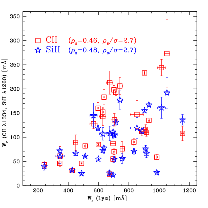
Figure 1: The rest-frame equivalent widths of the low-ionization metal lines (C ii and Si ii) against $W_{r}$(Ly$\alpha$). All the “weak” absorbers have $W_{r}(\mbox{Si\,{\sc ii}}\leavevmode\nobreak\ \lambda 1260)<200$ mÅ and $W_{r}(\mbox{C\,{\sc ii}}\leavevmode\nobreak\ \lambda 1334)<300$ mÅ by design. A mild $2.7\sigma$ correlation between $W_{r}(\mbox{C\,{\sc ii}},\mbox{Si\,{\sc ii}})$ and $W_{r}$(Ly$\alpha$) is present. An upper envelope with an apparent lack of data points in the upper-left corner (i.e. the region with $W_{r}$(Ly$\alpha$) $<600$ mÅ and $W_{r}(\mbox{C\,{\sc ii}},\mbox{Si\,{\sc ii}})>100$ mÅ) is evident.

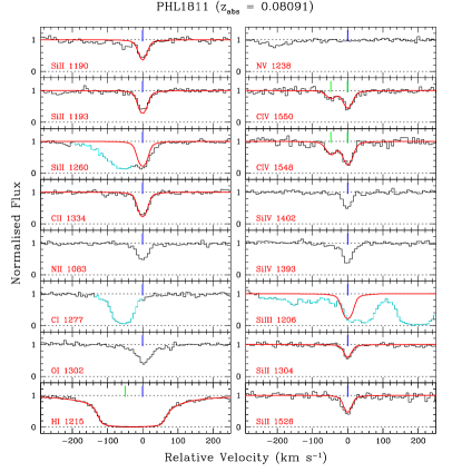
Figure 2: Velocity plot of a weak absorber at $z_{\rm abs}$ $=$ 0.08091 detected towards PHL1811. The smooth solid red curves over-plotted on top of data (black histogram) are the best fitting model profiles. Unrelated absorption lines are shown in cyan. Since the Si iii line is blended with the Galactic Si ii$\lambda 1304$ line, we have generated a synthetic profile corresponding to the maximum allowed column density. Single component C ii and Si ii lines are detected at $\sim 0$ km s^-1. The C iv absorption shows another component at $\sim-50$ km s^-1. Both the C iv and Ly$\alpha$ lines are fitted with two Voigt profile components. The line centroids of the individual components are marked by the vertical ticks in each panel. Velocity plots, Voigt profile fits, and comments about each absorbers can be found in Appendix C as online material.

2.2 Search techniques and the sample

Our search for the weak absorbers relies on the simultaneous presence of the Si ii$\lambda 1260$ and C ii$\lambda 1334$ lines. Note that the presence of C ii$\lambda 1334$ restricts our survey to a maximum redshift of $z_{\rm max}\approx 0.35$. First, we assume every detected absorption in a spectrum above $\lambda_{\rm obs}>1260$ Å is due to the Si ii$\lambda 1260$ line from redshift $z_{\rm abs}$ $=(\lambda_{\rm obs}/\lambda_{\rm rest})-1$, where $\lambda_{\rm rest}$ is the rest-frame wavelength of the Si ii$\lambda 1260$ transition . Next we check for the presence of the corresponding C ii$\lambda 1334$ line using the $z_{\rm abs}$. We build a “primary” list of absorbers using each of the identified coincidence. We then check for the presence of other common transitions ( e.g., Ly$\alpha$, Si ii$\lambda 1193$, C ii$\lambda 1036$, Si iii). Since some amount of neutral hydrogen is expected to be associated with these weak low-ionization absorbers, we have excluded any “primary” system that does not exhibit any detectable Ly$\alpha$ absorption. The presence of other metal lines would depend on the phase structure, ionization parameter, and metallicity of the absorber. We, therefore, do not impose the detection of any other metal line as a necessary criterion to confirm a weak absorber. Next, we investigate if the identified Si ii$\lambda 1260$ and$/$or C ii$\lambda 1334$ lines can have any other identity (i.e. other lines from other redshifts). We include a system in our “secondary” list when both the lines are free from significant contamination.

For each absorber in the “secondary” list we measure rest-frame equivalent widths ($W_{r}$) of Si ii$\lambda 1260$ and C ii$\lambda 1334$ lines. We consider only systems in which both the lines are detected with $\geqslant 3\sigma$ significance. Next we impose the $W_{r}$ threshold criteria so that each system in our final sample, listed in Table 1, has $W_{r}(\mbox{Si\,{\sc ii}}\lambda 1260)<200$ mÅ and $W_{r}(\mbox{C\,{\sc ii}}\lambda 1334)<300$ mÅ. The equivalent widths of the C ii and Si ii lines of our final sample are plotted against the $W_{r}$(Ly$\alpha$) in Fig. 1. A mild correlation between the equivalent widths of low-ionization metal lines and Ly$\alpha$ is apparent. A Spearman rank correlation test suggests a correlation coefficient, $\rho_{s}$, of $\approx 0.47$ with a $2.7\sigma$ significance. We notice an upper envelope in the figure which is likely due to a metallicity effect. In particular, the systems with $W_{r}$(Ly$\alpha$) $\lesssim 600$ mÅ would require unreasonably high metallicities in order to produce Si ii and/or C ii absorption with $W_{r}\gtrsim$ 100 mÅ. The systems with $W_{r}$(Ly$\alpha$) $>600$ mÅ, on the other hand, show a wide range in Si ii and C ii equivalent widths. This could be because of poor small scale metal mixing so that the observed H i need not entirely be associated with the low-ionization metal line (e.g., Schaye et al., 2007). This is certainly the case for systems for which the H i is not centered in velocity around the low ionization absorption (see e.g., Fig. 2).

The Si ii/C ii systems that show $W_{r}$ higher than our thresholds, i.e. the strong absorbers, are listed in Table 3 for completeness. The systems with $z_{\rm abs}$ within 5000 km s^-1 of the emission redshift ($z_{\rm em}$) of the background AGN$/$QSOs, as listed in Table 4, are excluded for this study since they might have different origins (see e.g., Muzahid et al., 2013) than the intervening absorbers we are interested in. Additionally, the systems with $cz<1000$ km s^-1 are not considered here, since they are likely to be related to our own Galaxy and$/$or local group galaxies. We refer the reader to Richter et al. (2016a) for a detailed analysis of such absorbers. There are a total of 34 weak Mg ii absorber analogs in our sample satisfying all of the above requirements.

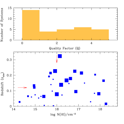
Figure 3: The absorption redshifts plotted against the $N(\mbox{H\,{\sc i}})$ values estimated for individual systems. The median values of $z_{\rm abs}$ and $\log N(\mbox{H\,{\sc i}})$ are indicated by the horizontal and vertical arrows, respectively. Symbol sizes are scaled by the corresponding quality factors ($Q$). The $Q$ distribution is shown in the top panel. In total there are 16 systems with $Q\geq 3$ for which $N(\mbox{H\,{\sc i}})$ estimates are reliable.

2.3 Absorption Line Measurements

Besides measuring equivalent widths, we used vpfit to obtain column densities of H i, Si ii, and C ii. The column densities of Si iii, C iv, and O vi are also measured whenever available. Since the line spread function (LSF) of the COS spectrograph is not a Gaussian, we use the LSF given by Kriss (2011). The LSF was obtained by interpolating the LSF tables at the observed central wavelength for each absorption line and was convolved with the model Voigt profile while fitting absorption lines or generating synthetic profiles. For fitting an absorption line, we have used the minimum number of components required to achieve a reduced $\chi^{2}\approx 1$. However, owing to the limited resolution of the COS spectrograph, we may be missing the “true” component structure. As a consequence, the Doppler parameters generally turn out to be larger compared to the high-$z$ weak absorbers detected in high-resolution $VLT/$UVES spectra (e.g., Narayanan et al., 2008). For a strong line this would lead to an underestimation of the corresponding column density. Nevertheless, the column density can be accurately measured for a weak line that falls on the linear part of the curve-of-growth (COG). COS wavelength calibration is known to have uncertainties at the level of $\approx 5-15$ km s^-1 (Savage et al., 2011; Muzahid et al., 2015a). We do see velocity misalignments of the same order between different absorption lines from the same system. An example of a weak absorber with the model profiles is shown in Fig. 2. System plots with Voigt profiles fits of the full sample are available in Appendix C.

3 Analysis

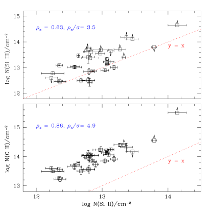
Figure 4: $\log N(\mbox{C\,{\sc ii}})$ versus $\log N(\mbox{Si\,{\sc ii}})$ (bottom) and $\log N(\mbox{Si\,{\sc iii}})$ versus $\log N(\mbox{Si\,{\sc ii}})$ (top) for each absorber. Note that $N(\mbox{Si\,{\sc ii}})$ is more tightly correlated with $N(\mbox{C\,{\sc ii}})$ as compared to $N(\mbox{Si\,{\sc iii}})$ in our sample. The $y=x$ (dotted) line is shown just for comparing the relative strengths of the low-ionization metal lines. The tight correlation between $N(\mbox{C\,{\sc ii}})$ and $N(\mbox{Si\,{\sc ii}})$ indicates that they trace the same phase of the absorbing gas. The somewhat larger scatter in the top panel possibly suggests that Si iii might have an additional contribution from the high-ionization gas phase for a fraction of the absorbers.

3.1 Absorber’s Frequency, $d\mathcal{N}/dz$

We have read through the titles and the abstracts of all the relevant program IDs, under which the 296 COS spectra were obtained, in order to inspect whether the spectra were taken to probe the CGM of known foreground galaxies. The spectra obtained from dedicated CGM programs (e.g. PID: 11598, 12248) were assigned to “flag = 0”, meaning that they are not part of our statistical sample. The remaining spectra with “flag = 1” constitute our statistical sample. There are 178 (118) “flag = 1” (“flag = 0”) spectra in our sample. The redshift path-length covered for simultaneously detecting Si ii$\lambda 1260$ ($\approx$0.2 Å) and C ii $\lambda 1334$ ($\approx$0.3 Å) in the 178 spectra in our statistical sample is $\Delta z=27.8$. There are 22 bona fide weak absorbers identified in these spectra (see Table 1). This yields the number density of weak absorbers, $d\mathcal{N}/dz=0.8\pm 0.2$ at $z<0.3$. This is consistent with the value ($1.00\pm 0.20$) obtained by Narayanan et al. (2005) using a much smaller sample size. We note that the $d\mathcal{N}/dz$ of H i absorbers (Danforth et al., 2016) with $N(\mbox{H\,{\sc i}})\approx 10^{16}$ cm^-2 at $z\approx 0.1$ (the median redshift of our sample) matches with that of the weak absorbers. Interestingly, the median $N(\mbox{H\,{\sc i}})$ in our sample is $10^{16}$ cm^-2, as we describe in the next section. This re-confirms the finding of Churchill et al. (1999) that the majority of the weak absorbers arise in a sub-LLS environment.

Recently Richter et al. (2016b) have presented a sample of Si iii absorbers at similar redshift using archival COS spectra. They have found $d\mathcal{N}/dz$ of $2.5\pm 0.4$ for Si iii down to a $N(\mbox{Si\,{\sc iii}})$ of $10^{12.2}$ cm^-2. Comparing this to the frequency of weak absorbers, we suggest that roughly half of the Si iii population should show associated weak Si ii absorption. From the middle panel of Fig. 6 of Richter et al. (2016b), there are 24 Si ii absorbers with $W_{r}(\mbox{Si\,{\sc ii}}\lambda 1260)<200$ mÅ. This leads to a $d\mathcal{N}/dz$ of $1.0\pm 0.2$ (using $\Delta z=24$ for their sample) which is consistent with our estimate.

In Table 1, there are 12 absorbers that are detected in the “flag = 0” spectra. We did not use them for the $d\mathcal{N}/dz$ calculation in order to avoid any possible observational bias. However, those systems are considered in all other analyses related to the chemical/physical conditions of the absorbing gas.

3.2 Neutral Hydrogen Column Density, $N(\mbox{H\,{\sc i}})$

Owing to the low redshifts of the weak absorbers ($z<0.3$), higher order Lyman series lines are not covered by the COS spectra for most cases. 17/34 systems have only Ly$\alpha$ and 7/34 systems have both Ly$\alpha$ and Ly$\beta$ coverages. The remaining 10 systems have Ly$\alpha$, Ly$\beta$, and Ly$\gamma$ (or higher order lines) coverages. Estimating reliable $N(\mbox{H\,{\sc i}})$ values in the absence of unsaturated higher order Lyman series lines is challenging. We, thus, assign a quality factor “$Q$” for each of our $N(\mbox{H\,{\sc i}})$ measurements based on the absorption strength (level of saturation) and the presence (or absence) of the higher order lines. The quality factor can take values from 1–5, with 5 being the best/secure measurements. $N(\mbox{H\,{\sc i}})$ values with $Q=1$ and $2$ are not well constrained. For each absorber listed in Table 1, we checked the literature to see if a $N(\mbox{H\,{\sc i}})$ measurement is available from fuse data. For 7 systems we have adopted $N(\mbox{H\,{\sc i}})$ values from the literature that were well constrained from higher-order Lyman series lines covered by the fuse spectra. These systems are $z_{\rm abs}$ $=0.22597$ towards HE0153-4520 (Savage et al., 2011), $z_{\rm abs}$ $=0.16710$ towards PKS0405-123 (Prochaska et al., 2004), $z_{\rm abs}$ $=0.13850$ towards PG1116+215 (Sembach et al., 2004), $z_{\rm abs}$ $=0.06350$ towards 3C263 (Savage et al., 2012), $z_{\rm abs}$ $=0.09495$ towards PKS1302-102 (Cooksey et al., 2008), $z_{\rm abs}$ $=0.07774$ towards PHL1811 (Lacki & Charlton, 2010), and $z_{\rm abs}$ $=0.08091$ towards PHL1811 (Jenkins et al., 2005). There are 3 additional systems for which we have adopted $N(\mbox{H\,{\sc i}})$ values from the literature. These systems are $z_{\rm abs}$ $=0.22722$ towards Q0107–025A (Muzahid, 2014), $z_{\rm abs}$ $=0.21451$ towards SDSSJ1322+4645, and $z_{\rm abs}$ $=0.17885$ towards SDSSJ1419+4207. The $N(\mbox{H\,{\sc i}})$ estimates for the latter two systems are obtained from the Lyman limit breaks seen in the G140L, G130/1222 grating observations using COS (see Prochaska et al., 2017). For all of these 10 systems we assign $Q\geq 3$. The absorption redshifts and $N(\mbox{H\,{\sc i}})$ estimates are shown in Fig. 3. The median $N(\mbox{H\,{\sc i}})$ is $10^{16.0}$ cm^-2 for the full sample. The median value becomes $10^{15.9}$ cm^-2 for the systems with $Q\geq 3$. The median value of redshifts changes from $0.12$ to $0.22$ when we consider the systems with $Q\geq 3$ as opposed to the full sample. This follows from the fact that the most of the lower redshift systems do not have higher order Lyman series lines covered.

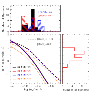
Figure 5: Bottom: cloudy predicted Si iii to Si ii ratios against the gas density for two different metallicities as indicated by the two different line styles. For each metallicity, four different models are run corresponding to four different $N(\mbox{H\,{\sc i}})$ values as shown by different colors. Clearly, the ratio is degenerate with respect to the assumed model metallicity. The distribution of observed $N(\mbox{Si\,{\sc iii}})/N(\mbox{Si\,{\sc ii}})$ ratio is shown in the right panel. Top: The density distribution corresponding to the observed $N(\mbox{Si\,{\sc iii}})/N(\mbox{Si\,{\sc ii}})$ ratio distribution for the two different model metallicities. The solid black histogram indicates the final density distribution after correcting for the metallicity degeneracies (see text).

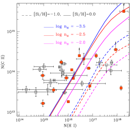
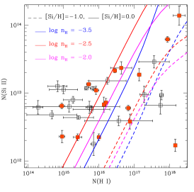
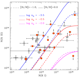
Figure 6: The C ii (left), Si ii (middle), and Si iii (right) column densities against $N(\mbox{H\,{\sc i}})$, as measured in different systems. The filled squares represent systems with $Q\geq 3$. The PI model curves corresponding to two different metallicities are shown in two different line-styles. For each model, we show three curves in three different colors corresponding to three representative densities (i.e., $\log n_{\rm H}=-2.0,-2.5,\&-3.5$).

3.3 Metal Column Densities

Besides H i, we have measured the column densities of C ii, Si ii, Si iii, C iv and O vi when available. All the measured total column densities (i.e. the sum of the component column densities) are listed in Table 2. The systems in our sample are weak by design and therefore it is expected that the C ii and Si ii lines are not saturated in most cases. In fact, for 29/34 cases we could measure the $N(\mbox{C\,{\sc ii}})$ adequately. The minimum and maximum values of $\log N(\mbox{C\,{\sc ii}})/\rm cm^{-2}$ for these systems are 13.22 and 14.40, respectively, with a median value of 13.9. The median value increases only by $\approx 0.1$ dex for the full sample. For all 34 systems we could measure $N(\mbox{Si\,{\sc ii}})$ reliably. The minimum and maximum values of $\log N(\mbox{Si\,{\sc ii}})/\rm cm^{-2}$ are 12.23 and 14.14, respectively, with a median value of 12.9. The median value of $N(\mbox{Si\,{\sc ii}})$ is an order of magnitude lower than that of $N(\mbox{C\,{\sc ii}})$.

Owing to the large $f_{\rm osc}\lambda_{\rm rest}$ value (i.e. 2027) of the Si iii$\lambda 1206$ transition, the Si iii absorption lines in our sample are saturated for nearly half (15/32) of the systems. We note that for two systems (i.e. $z_{\rm abs}$ $=0.06376$ towards UKS-0242-724 and $z_{\rm abs}$ $=0.07407$ towards SDSSJ1214+0825) Si iii lines fall in the spectral gap and hence no $N(\mbox{Si\,{\sc iii}})$ information is available. The minimum and maximum values of $\log N(\mbox{Si\,{\sc iii}})/\rm cm^{-2}$ are, respectively, 12.43 and 13.47 for the 18 systems in which we could measure $N(\mbox{Si\,{\sc iii}})$ adequately. The median value of the $N(\mbox{Si\,{\sc iii}})$ distribution is $10^{13.0}$ cm^-2, which is close to that of the $N(\mbox{Si\,{\sc ii}})$ distribution but a factor of $\approx 10$ smaller than the $N(\mbox{C\,{\sc ii}})$ distribution. The median value of $\log N(\mbox{Si\,{\sc iii}})/\rm cm^{-2}$ increases to $\approx 13.2$ for the full sample.

In the bottom panel of Fig. 4, the C ii column densities are plotted against $N(\mbox{Si\,{\sc ii}})$. Note that when multiple components are present, we have summed the component column densities. The $N(\mbox{C\,{\sc ii}})$ values are tightly correlated with $N(\mbox{Si\,{\sc ii}})$. A Spearman rank correlation test gives $\rho_{s}=0.86$ with a $4.9\sigma$ significance. If we consider only systems in which both $N(\mbox{C\,{\sc ii}})$ and $N(\mbox{Si\,{\sc ii}})$ are measured adequately (i.e. excluding the limits) we obtain $\rho_{s}=0.81$ with a $4.4\sigma$ significance. The strong correlation coefficient ensures that the C ii and Si ii arise from the same phase of the absorbing gas.

In the top panel of Fig. 4, the Si iii column densities are plotted against $N(\mbox{Si\,{\sc ii}})$. A statistically significant correlation between $N(\mbox{Si\,{\sc iii}})$ and $N(\mbox{Si\,{\sc ii}})$, with $\rho_{s}=0.63$ ($3.5\sigma$), is apparent from the figure. Nevertheless, there is more scatter in this plot compared to the bottom panel ($N(\mbox{C\,{\sc ii}})$ vs $N(\mbox{Si\,{\sc ii}})$). It is likely due to the fact that some amount of Si iii might be contributed by the high-ionization gas phase giving rise to C iv/O vi absorption for at least some fraction of the systems. We will discuss this issue in more detail in the following section.

3.4 Ionization Modeling

We use the photoionization (PI) simulation code cloudy (v13.03, last described by Ferland et al., 2013) to infer the overall physical and chemical properties of the weak absorbers in our sample. In our constant density PI models, we have assumed that (a) the absorbing gas has a plane parallel geometry, (b) the gas is subject to the extragalactic UV background (UVB) radiation at $z=0.1$ as computed by Khaire & Srianand (2015a, KS15 hereafter), (c) the relative abundances of heavy elements in the absorbing gas are similar to the solar values as measured by Asplund et al. (2009), and (d) the gas is dust free. Models are run for two different gas-phase metallicities, i.e., $\rm[X/H]=-1.0$ and $\rm[X/H]=0.0$. The KS15 UVB calculations make use of an updated QSO emissivity and star-formation rate density (see Khaire & Srianand, 2015b, for details). Their models with escape fraction (of H i ionizing photons from galaxies, $f_{\rm esc}$) of $0\%$ provide H i photoionization rates ($\Gamma_{\mbox{H\,{\sc i}}}$) at $z<0.5$ that are consistent with the measurements of Shull et al. (2015) and Gaikwad et al. (2016). We therefore use their model corresponding to $f_{\rm esc}=0\%$.

PI models for all the absorbers are done in a uniform fashion. First, we assume that the Si ii and Si iii absorption lines originate in the same phase of the absorbing gas and hence the ratio of $N(\mbox{Si\,{\sc iii}})/N(\mbox{Si\,{\sc ii}})$ uniquely fixes the $\log U$ (or $\log n_{\rm H}$) of the absorber. We, however, note that the Si iii need not entirely stem from the low-ionization gas phase that produces Si ii. If some amount of Si iii arise from high-ionization gas phase, the Si iii to Si ii ratio would provide an upper limit on the ionization parameter (a lower limit on density). Next, we use the ionization corrections of H i and Si ii ($f_{\mbox{H\,{\sc i}}}$ and $f_{\mbox{Si\,{\sc ii}}}$, respectively) at the derived $n_{\rm H}$ and calculate the Si abundance, [Si/H] $=\log N(\mbox{Si\,{\sc ii}})/N(\mbox{H\,{\sc i}})-\log f_{\mbox{Si\,{\sc ii}}}/f_{\mbox{H\,{\sc i}}}-\log{\rm(Si/H)_{\odot}}$, of the absorber using the observed $N(\mbox{H\,{\sc i}})$ and $N(\mbox{Si\,{\sc ii}})$. The $f_{\mbox{Si\,{\sc ii}}}/f_{\mbox{H\,{\sc i}}}$ ratio shows a relatively flat peak for a large range in density of $\rm 10^{-3.4}-10^{-2.4}cm^{-3}$, and falls off rapidly at both below and above this density range. Thus, even if the measured $N(\mbox{Si\,{\sc iii}})$ has some contribution from a high ionization gas phase, our inferred metallicity will essentially be unaltered (see also Section 5.3).

4 Results based on the PI models

4.1 The density (ionization parameter) distribution

In the bottom panel of Fig. 5 we show the variation of the model predicted $N(\mbox{Si\,{\sc iii}})/N(\mbox{Si\,{\sc ii}})$ ratio with density for two different model metallicities, i.e., solar and 1/10th of solar values. We note that the $N(\mbox{Si\,{\sc iii}})/N(\mbox{Si\,{\sc ii}})$ ratio depends on the metallicity assumed in the cloudy model. This is likely due to the increased electron density in high metallicity gas increasing the recombination/cooling rate for a fixed density and temperature. For each model metallicity we have used four different $\log N(\mbox{H\,{\sc i}})/\rm cm^{-2}$ values (i.e., 15, 16, 17, and 18) as the stopping conditions for the simulations. Note that, for a given metallicity, the ratio is independent of the $N(\mbox{H\,{\sc i}})$ values as long as the gas is optically thin to the hydrogen ionizing photons (i.e., $N(\mbox{H\,{\sc i}})\lesssim 10^{17.2}$ cm^-2). We, however, used the observed $N(\mbox{H\,{\sc i}})$ values as stopping conditions for cloudy for each of the absorbers in order to derive individual constraints.

[t] QSO $z_{\rm abs}$ $\log N(\mbox{H\,{\sc i}})$ $\log N(\mbox{C\,{\sc ii}})$ $\log N(\mbox{Si\,{\sc ii}})$ $\log N(\mbox{Si\,{\sc iii}})$ $Q$ $\log n_{\rm H}(U)$ $\rm[Si/H]$ $\log N_{\rm H}$ $L$ $\log N(\mbox{C\,{\sc iv}})$ $\log N(\mbox{O\,{\sc vi}})$ $\log N(\mbox{Mg\,{\sc ii}})$ $\rm(1/cm^{-3})$ $\rm(1/cm^{-2})$ (kpc) (observed) (model) (observed) (model) (model) PG0003+158 0.16512 18.16 $\pm$ 0.03 13.60 $\pm$ 0.05 12.23 $\pm$ 0.09 $<$12.60 3 $-$2.9 ($-$3.1) $-$2.5 19.9 2.02E+01 NA 12.2 13.82 $\pm$ 0.12 9.7 11.8 Q0107-025A 0.22722 15.92 $\pm$ 0.08 13.85 $\pm$ 0.07 13.04 $\pm$ 0.06 12.90 $\pm$ 0.05 5 $-$2.6 ($-$3.4) 0.2 17.7 6.91E-02 14.24 $\pm$ 0.12^a 12.4 14.57 $\pm$ 0.23 9.2 12.4 HE0153-4520 0.22597 16.83 $\pm$ 0.07 14.09 $\pm$ 0.03 12.78 $\pm$ 0.04 $>$13.73 4 $-$3.1 ($-$2.9) $-$0.7 19.2 6.34E+00 NA 13.9 14.24 $\pm$ 0.02 11.9 12.3 3C57 0.32338 16.14 $\pm$ 0.02 14.05 $\pm$ 0.02 12.83 $\pm$ 0.11 $>$13.61 5 $-$3.3 ($-$2.7) 0.0 18.6 2.47E+00 NA 14.2 $<$13.4 12.6 12.2 SDSSJ0212-0737 0.01603 18.27 $\pm$ 0.17 $>$15.50 14.14 $\pm$ 0.14 $>$14.65 3 $-$3.1 ($-$2.9) $-$0.7 20.2 5.33E+01 15.03 $\pm$ 0.25 14.5 NA 12.3 13.8 SDSSJ0212-0737 0.13422 14.95 $\pm$ 0.08 13.91 $\pm$ 0.10 12.81 $\pm$ 0.04 12.43 $\pm$ 0.15 3 $-$2.5 ($-$3.5) 0.9 16.6 3.59E-03 $<$13.4 11.8 $<$13.7 8.1 12.2 UKS-0242-724 0.06376 15.27$\pm$0.27 13.73 $\pm$ 0.09 12.90 $\pm$ 0.05 NA 1 … … … … $<$13.3 … NA … … Q0349-146 0.07256 16.24 $\pm$ 0.53 13.91 $\pm$ 0.09 13.18 $\pm$ 0.05 13.01 $\pm$ 0.09 1 $-$2.6 ($-$3.4) 0.0 18.0 1.34E-01 $<$13.5 12.5 NA 9.3 12.5 PKS0405-123 0.16710 16.45 $\pm$ 0.05 $>$14.40 13.33 $\pm$ 0.03 $>$13.40 5 $-$2.8 ($-$3.2) $-$0.1 18.4 4.56E-01 14.16 $\pm$ 0.05^b 13.1 14.73 $\pm$ 0.13 10.3 12.7 IRAS-F04250-5718 0.00369 15.85 $\pm$ 0.08 13.49 $\pm$ 0.04 12.25 $\pm$ 0.17 12.78 $\pm$ 0.06 1 $-$3.1 ($-$2.9) $-$0.4 18.1 4.92E-01 13.21 $\pm$ 0.15 13.0 NA 10.9 11.6 FBQS-0751+2919 0.20399 17.77 $\pm$ 0.05 14.23 $\pm$ 0.06 12.97 $\pm$ 0.07 $>$13.55 2 $-$2.8 ($-$3.2) $-$1.5 19.8 1.40E+01 NA 13.1 14.35 $\pm$ 0.07 10.5 12.6 VV2006J0808+0514 0.02930 17.56 $\pm$ 0.43 $<$14.17 13.46 $\pm$ 0.09 $>$14.11 1 $-$2.8 ($-$3.2) $-$0.8 19.7 9.66E+00 NA 13.7 NA 11.1 13.1 PG0832+251 0.02811 14.28 $\pm$ 0.14 13.56 $\pm$ 0.08 12.79 $\pm$ 0.10 12.51 $\pm$ 0.11 2 $-$2.5 ($-$3.5) 1.6 16.0 1.01E-03 $<$13.3 11.9 NA 8.5 12.2 SDSSJ0929+4644 0.06498 14.67 $\pm$ 0.71 13.50 $\pm$ 0.11 12.68 $\pm$ 0.06 12.50 $\pm$ 0.09 2 $-$2.6 ($-$3.4) 1.1 16.4 3.35E-03 $<$13.1 12.0 NA 8.7 12.0 PMNJ1103-2329 0.08352 17.74 $\pm$ 0.44 14.03 $\pm$ 0.10 12.82 $\pm$ 0.13 $>$13.37 1 $-$2.8 ($-$3.2) $-$1.6 19.7 1.15E+01 14.43 $\pm$ 0.06 12.9 NA 10.2 12.5 PG1116+215 0.13850 16.20 $\pm$ 0.05 13.84 $\pm$ 0.02 12.86 $\pm$ 0.06 12.87 $\pm$ 0.03 5 $-$2.7 ($-$3.3) $-$0.3 18.1 2.07E-01 13.19 $\pm$ 0.08 12.5 13.84 $\pm$ 0.02 9.6 12.2 SDSSJ1122+5755 0.05319 15.16 $\pm$ 1.43 13.56 $\pm$ 0.13 12.80 $\pm$ 0.08 12.85 $\pm$ 0.11 1 $-$2.7 ($-$3.3) 0.7 17.1 2.03E-02 13.71 $\pm$ 0.15 12.5 NA 9.6 12.1 PG1121+422 0.19238 15.64 $\pm$ 0.05 14.12 $\pm$ 0.02 13.07 $\pm$ 0.02 13.34 $\pm$ 0.06 2 $-$2.9 ($-$3.1) 0.5 17.7 1.26E-01 NA 13.2 $<$13.4 10.8 12.4 3C263 0.06350 15.40 $\pm$ 0.12 13.55 $\pm$ 0.06 12.35 $\pm$ 0.05 13.09 $\pm$ 0.02 4 $-$3.2 ($-$2.8) 0.3 17.8 3.66E-01 14.13 $\pm$ 0.15 13.6 NA 11.9 11.8 PG1202+281 0.13988 15.73 $\pm$ 0.10 14.04 $\pm$ 0.17 12.79 $\pm$ 0.09 13.41 $\pm$ 0.24 1 $-$3.1 ($-$2.9) 0.3 18.1 5.15E-01 $<$13.9 13.8 $<$13.6 11.8 12.2 PG-1206+459 0.21439 15.71 $\pm$ 0.06 14.24 $\pm$ 0.05 13.13 $\pm$ 0.05 $<$13.65 3 $-$3.1 ($-$2.9) 0.6 18.0 3.44E-01 NA 13.9 NA 11.8 12.5 SDSSJ1210+3157 0.05974 14.83 $\pm$ 0.27 14.06 $\pm$ 0.05 13.10 $\pm$ 0.08 13.23 $\pm$ 0.11 1 $-$2.8 ($-$3.2) 1.3 16.8 1.23E-02 14.50 $\pm$ 0.10 13.0 NA 10.2 12.4 SDSSJ1210+3157 0.14964 17.28 $\pm$ 0.12 14.23 $\pm$ 0.11 12.98 $\pm$ 0.12 $>$13.69 1 $-$2.8 ($-$3.2) $-$1.0 19.4 5.95E+00 14.35 $\pm$ 0.13 13.4 14.72 $\pm$ 0.11 10.8 12.6 SDSSJ1214+0825 0.07407 15.00 $\pm$ 0.40 14.13 $\pm$ 0.07 13.05 $\pm$ 0.06 NA 1 … … … … NA … NA … … RXJ1230.8+0115 0.00575 15.42 $\pm$ 0.43 13.79 $\pm$ 0.01 12.64 $\pm$ 0.02 13.47 $\pm$ 0.07 1 $-$3.3 ($-$2.7) 0.6 17.9 5.48E-01 13.32 $\pm$ 0.19 14.2 NA 12.6 12.0 PKS1302-102 0.09495 16.88 $\pm$ 0.03 13.65 $\pm$ 0.09 12.58 $\pm$ 0.11 13.02 $\pm$ 0.06 4 $-$2.6 ($-$3.4) $-$1.1 18.8 7.78E-01 $<$13.0 12.3 $<$13.9 9.2 12.2 SDSSJ1322+4645 0.21451 17.14 $\pm$ 0.05 14.40 $\pm$ 0.05 13.27 $\pm$ 0.09 $>$13.71 4 $-$2.6 ($-$3.4) $-$0.6 19.0 1.46E+00 NA 13.0 14.55 $\pm$ 0.08 9.9 12.9 SDSSJ1357+1704 0.09784 15.79 $\pm$ 0.52 13.97 $\pm$ 0.04 12.76 $\pm$ 0.05 $>$13.64 1 $-$3.3 ($-$2.7) 0.4 18.3 1.60E+00 13.92 $\pm$ 0.12 14.4 $<$14.1 13.0 12.2 SDSSJ1419+4207 0.17885 16.63 $\pm$ 0.30 14.32 $\pm$ 0.14 13.37 $\pm$ 0.09 $>$14.18 4 $-$3.3 ($-$2.7) 0.1 19.2 9.34E+00 NA 14.9 14.43 $\pm$ 0.05 13.2 12.8 PG1424+240 0.12126 14.96 $\pm$ 0.08 13.22 $\pm$ 0.08 12.36 $\pm$ 0.09 12.46 $\pm$ 0.10 3 $-$2.8 ($-$3.2) 0.4 16.9 1.50E-02 13.70 $\pm$ 0.06 12.2 14.44 $\pm$ 0.05 9.4 11.7 PG1424+240 0.14683 16.56 $\pm$ 0.96 13.71 $\pm$ 0.06 12.59 $\pm$ 0.07 13.04 $\pm$ 0.05 1 $-$2.6 ($-$3.4) $-$0.7 18.5 3.84E-01 14.18 $\pm$ 0.06 12.4 14.04 $\pm$ 0.13 9.3 12.2 PG-1630+377 0.17388 15.83 $\pm$ 0.08 14.20 $\pm$ 0.03 13.07 $\pm$ 0.02 13.14 $\pm$ 0.02 1 $-$2.8 ($-$3.2) 0.3 17.7 1.03E-01 NA 12.8 13.86 $\pm$ 0.03 10.0 12.4 PHL1811 0.07774 16.00 $\pm$ 0.05 13.26 $\pm$ 0.03 12.35 $\pm$ 0.05 12.48 $\pm$ 0.04 5 $-$2.4 ($-$3.6) $-$0.4 17.6 3.24E-02 $<$13.0 11.4 NA 6.6 11.9 PHL1811 0.08091 17.94 $\pm$ 0.07 $>$14.55 13.79 $\pm$ 0.04 $<$13.80 4 $-$2.5 ($-$3.5) $-$0.8 19.4 2.42E+00 14.04 $\pm$ 0.04 12.8 NA 8.9 13.3

Table 2: Summary of column density measurements and photoionization model parameters.

• Notes–
  No ionization model is done for the $z_{\rm abs}$ $=$ 0.06376 towards UKS-0242-724 and $z_{\rm abs}$ $=$ 0.07407 towards SDSSJ1214+0825 systems due to the lack of the $N(\mbox{Si\,{\sc iii}})$ measurements.
  “NA” indicates that the line is either severely blended or not covered by the corresponding COS spectrum.
  The last column gives the predicted Mg ii column densities. The model predicted $N(\mbox{Mg\,{\sc ii}})$ values reassure that these are indeed analogs of weak Mg ii absorbers (see also Appendix A).
  While assigning formal $1\sigma$ confidence intervals in the inferred densities and metallicities is not straightforward, we find that our metallicity estimates are adequate within $0.2$ dex, provided that the $N(\mbox{H\,{\sc i}})$ estimates are accurate (see Section 5.3). The densities are very sensitive to the metallicity assumed in the cloudy grid, particularly for the metal-rich systems. We find that the densities can be off by a factor of $\approx$3–4.
  ^aFrom Muzahid (2014), ^bFrom Savage et al. (2010).

The red (135${}^{{}^{\circ}}$) hashed histogram in the top panel of Fig. 5 represents the $\log n_{\rm H}$ distribution corresponding to the observed $N(\mbox{Si\,{\sc iii}})/N(\mbox{Si\,{\sc ii}})$ ratios, shown in the bottom-right panel, for an assumed metallicity of $\rm[X/H]=0.0$. The blue (45${}^{{}^{\circ}}$) hashed histogram, on the other hand, represents the same for an assumed metallicity of $\rm[X/H]=-1.0$. Clearly, an assumption of any particular model metallicity for all the absorbers in a sample leads to an incorrect density distribution. In order to overcome this problem we have performed our PI modelling in an iterative way. First, we used the density solution corresponding to the $\rm[X/H]=-1.0$ model and calculate the Si abundances for each absorber. We then select the systems with $\rm[Si/H]>-0.3$ (i.e. half solar) and redo the density calculation using the $\rm[X/H]=0.0$ model. The distribution of our final density solutions is shown by the black histogram in the top panel of Fig. 5. The $\log n_{\rm H}/\rm cm^{-3}$ distribution has a median value of $-2.8$ with minimum and maximum values of $-3.3$ and $-2.4$, respectively. For the adopted UVB, this leads to a range in ionization parameter, $\log U$, of $-2.7$ to $-3.6$ with a median value of $-3.2$.

4.2 The column density trends

In the different panels of Fig. 6, column densities of low-ionization metal lines are plotted against the corresponding $N(\mbox{H\,{\sc i}})$. A mild trend of increasing low-ionization metal line column densities with increasing $N(\mbox{H\,{\sc i}})$ is noticeable. A similar trend has also been reported for the COS-Halos sample (i.e., Werk et al., 2013; Prochaska et al., 2017). A Spearman rank correlation analysis, assuming limits are detections, also confirms the trends with a $\rho_{s}\gtrsim 0.3$ when the full sample is considered (see Table 3). It is important to note that when we consider the sub-sample with $N(\mbox{H\,{\sc i}})>10^{16}$ cm^-2 (median value), the correlation coefficients remain high (i.e. $\rho_{s}\gtrsim 0.2$). The sub-sample with $N(\mbox{H\,{\sc i}})\leq 10^{16}$ cm^-2, on the contrary, show $\rho_{s}$ consistent with 0.0. Though the sample size is small, it seems that the mild trends seen in the full sample are mainly driven by the systems with $N(\mbox{H\,{\sc i}})>10^{16}$ cm^-2.

In each panel in Fig. 6, six different PI model curves, corresponding to two different metallicities and three different densities, are overplotted. Note that the three representative densities span the density range we obtained from the $N(\mbox{Si\,{\sc iii}})/N(\mbox{Si\,{\sc ii}})$ ratios as discussed above. It is apparent from the three panels that the majority of the systems with $\log N(\mbox{H\,{\sc i}})/\rm cm^{-2}<16.0$ are not reproduced by the models with $1/10$th of solar metallicity. Moreover, even the solar-metallicity-models fail to reproduce the systems with $\log N(\mbox{H\,{\sc i}})/\rm cm^{-2}<15.7$. It is, therefore, clear that the vast majority of the weak absorbers studied here have very high metallicities.

4.3 Trends in the model parameters

The PI model predicted densities ($n_{\rm H}$), Si-abundances ($\rm[Si/H]$), total hydrogen column densities ($N_{\rm H}$), and line of sight thicknesses ($L$) are listed in columns 8, 9, 10, and 11 of Table 2, respectively. As mentioned before, the densities of the absorbers show a range of $10^{-3.3}$–$10^{-2.4}$ $\rm cm^{-3}$ with a median value of $10^{-2.8}$ $\rm cm^{-3}$. The density range and the median value do not change when only $Q>2$ systems are considered. The inferred $\rm[Si/H]$ values show a range of $-2.5$ to $+1.6$ with a median value of $0.0$ (i.e. solar abundance). However, when we considered only $Q>2$ systems the maximum value drops to $\rm[Si/H]=0.9$ (i.e. $\approx 8$ times solar) and the median value becomes $-0.1$. The total hydrogen column densities for the weak absorbers show a range of 4 orders of magnitude, i.e., $N_{\rm H}=10^{16.0-20.3}$ cm^-2, with a median value of $10^{18.1}$ cm^-2. The line of sight thicknesses, $L$, also exhibit a wide range of 1 pc – 53 kpc with a median value of $\approx 500$ pc. The median value changes to $\approx 780$ pc for the systems with $Q>2$.

The PI model parameters are plotted against the observed column densities of H i (top row), C ii (middle row), and Si ii (bottom row) in Fig. 7. The inferred densities do not show any trend with the neutral hydrogen and/or low-ionization metal line column densities. No significant correlation is seen between $\rm[Si/H]$ and $N(\mbox{C\,{\sc ii}})$ or $N(\mbox{Si\,{\sc ii}})$. A strong anti-correlation ($\rho_{s}=-0.94$, $\rho_{s}/\sigma=-5.2$) between $\rm[Si/H]$ and $N(\mbox{H\,{\sc i}})$, however, is apparent from the figure. The trend remains statistically significant ($\rho_{s}=-0.89$, $\rho_{s}/\sigma=-3.5$) when only systems with $Q>2$ are considered. A similar trend has been recently reported by Prochaska et al. (2017) in the COS-Halos sample. Such a trend is generally expected in a metal line selected sample of absorbers, because, in practice, there are many low-$N(\mbox{H\,{\sc i}})$ systems without any detectable low-ionization metal lines that are not considered in our study. In order to investigate the dependence of the correlation on $N(\mbox{H\,{\sc i}})$, we have performed the Spearman rank correlation analysis for two different sub-samples, one with $N(\mbox{H\,{\sc i}})>10^{16}$ cm^-2 and the other with $N(\mbox{H\,{\sc i}})\leq 10^{16}$ cm^-2, separately. We obtain $\rho_{s}=-0.75$ and $\rho_{s}/\sigma=-2.9$ ($\rho_{s}=-0.89$ and $\rho_{s}/\sigma=-3.5$) for the upper-$N(\mbox{H\,{\sc i}})$ (lower-$N(\mbox{H\,{\sc i}})$) sub-samples, suggesting a statistically significant anti-correlation between $\rm[Si/H]$ and $N(\mbox{H\,{\sc i}})$ for the systems with $N(\mbox{H\,{\sc i}})>10^{16}$ cm^-2. Note that, $>$80% of the low-$z$ H i absorbers with $N(\mbox{H\,{\sc i}})>10^{16}$ cm^-2 exhibit low-ionization metal lines (see Fig. 8 in Danforth et al., 2016). Thus, the strong anti-correlation seen in the full sample cannot be fully attributed to sample selection bias (see also the discussion of Misawa et al., 2008). However, we do point out that our survey is limited to weak absorbers only. Inclusion of strong absorbers would introduce more scatter in the relation, particularly at the higher $N(\mbox{H\,{\sc i}})$ end.

The strong $5.2\sigma$ correlation between $N_{\rm H}$ and $N(\mbox{H\,{\sc i}})$ is not surprising since the expected variation in $f_{\mbox{H\,{\sc i}}}$ over the inferred narrow density range of $10^{-3.3}-10^{-2.4}$ cm^-3 is small and $N_{\rm H}$ ($\equiv N(\mbox{H\,{\sc i}})/f_{\mbox{H\,{\sc i}}}$) is directly proportional to $N(\mbox{H\,{\sc i}})$. The $4.7\sigma$ correlation between $L\leavevmode\nobreak\ (\equiv N_{\rm H}/n_{\rm H})$ and $N(\mbox{H\,{\sc i}})$ follows from the fact that $N_{\rm H}$ is strongly correlated with $N(\mbox{H\,{\sc i}})$ whereas $n_{\rm H}$ is not. The $N_{\rm H}$ also show a significant (mild) correlation with $N(\mbox{C\,{\sc ii}})$ ($N(\mbox{Si\,{\sc ii}})$). If the column density of the (i+1)-th ionization state of an element $\rm X$, with ionization fraction of $f_{{\rm X_{i}}}$, is $N({\rm X_{i}})$, then

$$N_{\rm H} = \frac{N({\rm X_{i}})}{f_{{\rm X_{i}}}10^{\rm[X/H]}{\rm(X/H)_{\odot}}}\leavevmode\nobreak\ ,{\rm and}$$ (1)

$$L = \frac{N({\rm X_{i}})}{f_{{\rm X_{i}}}10^{\rm[X/H]}{\rm(X/H)_{\odot}}n_{\rm H}}\leavevmode\nobreak\ .$$ (2)

Thus, a correlation between $N_{\rm H}$ (and/or $L$) and metal line column density is generally anticipated. Any anti-correlation between the metallicity ($\rm[X/H]$) and the ionic column density, as seen for C ii, would further strengthen the correlation. The apparent lack of any correlation between $\rm[Si/H]$ and $N(\mbox{Si\,{\sc ii}})$ has been manifested by the mild $1.6\sigma$ correlation seen between $N_{\rm H}$ and $N(\mbox{Si\,{\sc ii}})$ in contrast to the strong $3.0\sigma$ correlation seen between $N_{\rm H}$ and $N({\mbox{C\,{\sc ii}}})$.

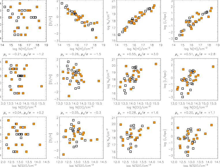
Figure 7: Scatter plots of PI model parameters ($\log n_{\rm H}$, 1st column; $\rm[Si/H]$, 2nd column, $\log N_{\rm H}$, 3rd column; $\log L$, 4th column) and the observed column densities ($N(\mbox{H\,{\sc i}})$, top row; $N(\mbox{C\,{\sc ii}})$, middle row; $N(\mbox{Si\,{\sc ii}})$, bottom row). The filled squares represent the systems with $Q>2$. The results of the Spearman rank correlation analysis are mentioned on the top of each panel. Possible origins of the observed correlations are discussed in the text. In particular, we argue that the $5.2\sigma$ anti-correlation seen between $\rm[Si/H]$ and $\log N(\mbox{H\,{\sc i}})$ cannot be entirely attributed to selection bias.

[b] Sample Data1 Data2 $\rho_{s}$ $\rho_{s}/\sigma$ Full $N(\mbox{H\,{\sc i}})$ $N(\mbox{C\,{\sc ii}})$ 0.48 2.8 Full $N(\mbox{H\,{\sc i}})$ $N(\mbox{Si\,{\sc ii}})$ 0.28 1.6 $N(\mbox{H\,{\sc i}})>10^{16}$ cm^-2 $N(\mbox{H\,{\sc i}})$ $N(\mbox{C\,{\sc ii}})$ 0.30 1.2 $N(\mbox{H\,{\sc i}})>10^{16}$ cm^-2 $N(\mbox{H\,{\sc i}})$ $N(\mbox{Si\,{\sc ii}})$ 0.20 0.8 $N(\mbox{H\,{\sc i}})\leq 10^{16}$ cm^-2 $N(\mbox{H\,{\sc i}})$ $N(\mbox{C\,{\sc ii}})$ 0.10 0.4 $N(\mbox{H\,{\sc i}})\leq 10^{16}$ cm^-2 $N(\mbox{H\,{\sc i}})$ $N(\mbox{Si\,{\sc ii}})$ $-0.12$ $-0.5$

Table 3: The details of Spearman rank correlation analysis

4.4 High-ionization metal lines

Although the main focus of this paper is the weak absorbers detected via the low-ionization metal lines, in all but a few cases high-ionization metal lines (e.g. C iv and/or O vi) are also covered. For example, $N(\mbox{C\,{\sc iv}})$ information is available for a total of 23 systems (15 measurements and 8 upper limits, see Table 2). All the upper limits on $N(\mbox{C\,{\sc iv}})$ are consistent with our PI model predictions. For the 15 systems with positive detection of C iv, the column densities are found to be in the range $10^{13.2-15.0}$ cm^-2 with a median value of $10^{14.1}$ cm^-2. Our $N(\mbox{C\,{\sc iv}})$ measurements are at least 0.5 dex higher than the model predicted values for 12/15 systems, suggesting a separate gas phase for C iv absorption in those absorbers. For the $z_{\rm abs}$ $=0.00369$ system towards IRAS-F04250-5718, the difference is only 0.2 dex, which is well within our PI model uncertainties. For the two other systems ($z_{\rm abs}$ $=0.00575$ towards RXJ1230.8+0115 and $z_{\rm abs}$ $=0.09784$ towards SDSSJ1357+1704) the model predicted C iv column densities are higher than the observed ones. In both these systems the Si iv line is detected. It is likely that the majority of the Si iii absorption in these systems arises from the gas phase giving rise to Si iv (and C iv) absorption. In that situation the ionization parameter of the low-ionization phase can be a lot lower which, in turn, will reduce the predicted $N(\mbox{C\,{\sc iv}})$. In the $z_{\rm abs}$ $=0.09784$ system towards SDSSJ1357+1704, the stronger Si iii component at $\approx 0$ km s^-1, which dominates the total $N(\mbox{Si\,{\sc iii}})$, is not seen in the low-ionization lines but is seen in the Si iv line (see Appendix C). We further note that the majority of systems for which the predicted $N(\mbox{C\,{\sc iv}})$ values are considerable (i.e. $>10^{14.0}$ cm^-2) show strong Si iv absorption. These facts demonstrate the need for component-by-component, multi-phase photoionization models (see e.g., Charlton et al., 2003; Milutinović et al., 2006; Misawa et al., 2008), which is beyond the scope of this paper.

The O vi doublet is covered for 18/34 of the weak absorbers, of which 12 show detectable absorption. The O vi column densities in these absorbers vary between $10^{13.8-14.7}$ cm^-2 with a median value of $10^{14.4}$ cm^-2. The maximum predicted $N(\mbox{O\,{\sc vi}})$ by our PI models (i.e., $10^{13.2}$ cm^-2) is 0.6 dex lower than the lowest measured $N(\mbox{O\,{\sc vi}})$ value. It clearly indicates that in all these systems O vi must originate from a separate gas phase. In 10/34 of the weak absorbers both the C iv and the O vi doublets are covered. In 6/10 cases both C iv and O vi are detected, and it is likely that they arise in the same gas phase. In one case ($z_{\rm abs}$ $=$ 0.09784 towards SDSSJ1357+1704 discussed in the paragraph above) only C iv is detected. Finally, in 3/10 cases neither C iv or O vi are detected. We conclude that about two thirds of the weak absorbers have a separate, higher ionization or hotter phase.

5 Discussion

5.1 Redshift Evolution

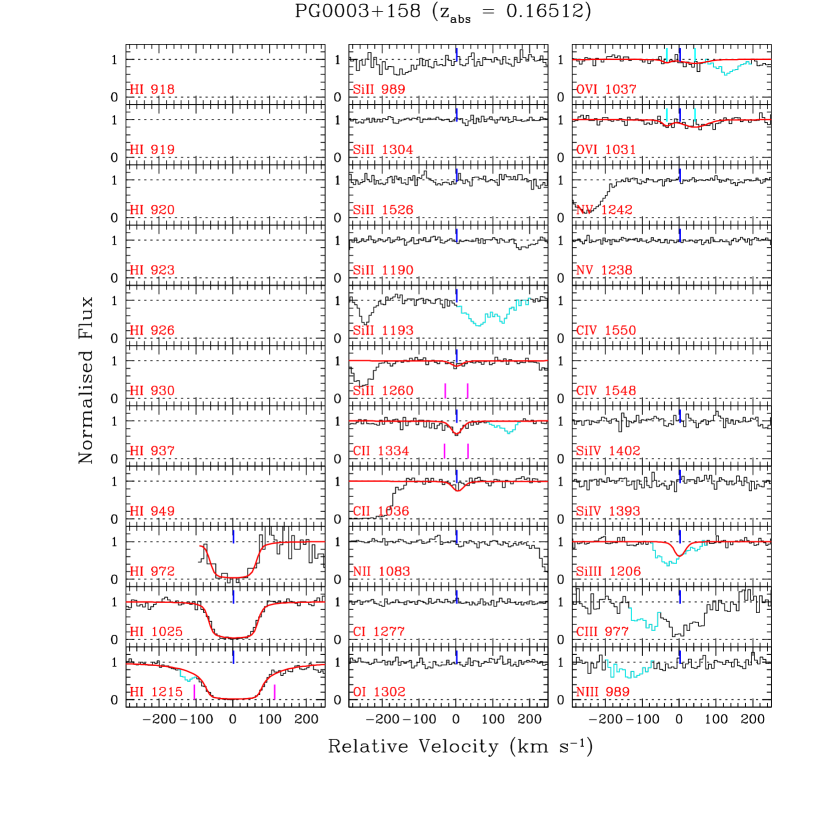
Figure 12: Velocity plot of the $z_{\rm abs}$ $=0.16512$ system towards QSO PG 0003$+$158. Relevant parts of the COS spectrum covering various important transitions from the absorber are shown on a velocity scale. The zero velocity corresponds to the absorption redshift, mentioned on the top. The smooth red curves overplotted on top of the data (black histogram) are the best fitting Voigt profile models. No data are displayed when a line is not covered by the COS spectrum. The blue vertical ticks mark the line centroids of the model Voigt profiles and the pairs of vertical magenta lines in Ly$\alpha$, Si ii$\lambda$1260, and C ii $\lambda$1334 panels mark the region over which $W_{r}$ of the corresponding line is measured. Unrelated absorption lines are shown in cyan. Very weak Si ii$\lambda 1260$ and C ii$\lambda 1334$ absorption lines are seen. The Si iii$\lambda 1206$ line is heavily blended with the Ly$\beta$ from the $z_{\rm abs}$ $=0.37037$ system. The Ly$\gamma$ and C iii$\lambda 977$ lines fall at the blue edge of the spectrum. Both the lines require a velocity shift of $\sim+30$ km s^-1 in order to be properly aligned with the other lines. The Ly$\beta$, C ii$\lambda 1036$, and O vi doublets, on the other hand, require a velocity shift of $\sim-10$ km s^-1. The C ii and Si ii lines are fitted simultaneously keeping the $z$ and Doppler-parameter ($b$) tied to each other. Since the Si iii line is blended, we estimate the maximum allowed column density, using a $z$ and $b$-parameter same as the C ii/Si ii line, that do not exceed the observed profile. The simultaneous and single component fit to the Lyman series lines explains the observed profiles adequately. We believe that the $N(\mbox{H\,{\sc i}})$ of $10^{18.16\pm 0.03}$ cm^-2 is adequately constrained from the wing of the Ly$\alpha$ line along with the Ly$\beta$ and Ly$\gamma$ profiles. We thus assign a quality factor of $Q=3$ for this system.

Our sample of 34 weak Mg ii absorber analogs at $z<0.3$ represents a substantial increase over the sample of 6 absorbers found by Narayanan et al. (2005) at low redshift. However, the value of $dN/dz=0.8\pm 0.2$ that we have derived is consistent with that earlier study, and a factor of a few smaller than what would be expected if static populations of weak Mg ii and C iv absorbers were simply evolved to the present era subject to the decreasing UVB. Narayanan et al. (2005) noted that both pc-scale structures that produce weak Mg ii absorption at $z\approx 1$ and kpc-scale structures that are detected in C iv absorption, but not in low ionization transitions, would evolve from $z\approx 1$ to produce weak low ionization absorption at $z\approx 0.1$. To some extent, both populations must be less abundant at low redshift than they were at $z\approx 1$. The present sample of 34 absorbers is large enough that we can attempt to determine how the low redshift population compares to the $z\approx 1$ population, however Narayanan et al. (2005) warned that “hidden phases” would in some cases make it impossible to extract accurate physical properties (see their Figs. 10–12).

We begin by noting that 7/34 of our weak absorbers are very small ($<32$ pc) structures with solar or super-solar metallicity and with derived densities $\log n_{\rm H}/\rm cm^{-3}\approx-2.6$ in the upper half of our sample. Although these overlap with the densities derived by Narayanan et al. (2008) for weak Mg ii absorbers (using coverage of Fe ii to constrain density), they are at the low end of the range. All but one of these seven small absorbers has only one low ionization component, and C iv is either not detected at all (in 4/7) or it could be in the same phase with, and centered on the low ionization absorption. Even these absorbers, for which the metallicity is inferred to be quite high, could have two phases that contribute roughly equally to the Si ii/C ii absorption, as in the simulated system in Fig. 11 of Narayanan et al. (2005). However, it is still clear that there is a smaller, higher density phase which has a surprisingly high metallicity.

Furthermore, many of the remaining 27/34 absorbers, though they have larger derived line of sight thicknesses based on our conservative estimates, are likely to have a hidden phase. The inferred density of that phase would be higher than we estimate if some of the Si iii is in fact in a lower density phase that produced C iv absorption. The inferred metallicity of that phase would be higher if some of the H i is associated with the higher ionization transitions, C iv and/or O vi.

Thus, despite our larger sample, the situation remains unclear. We can, however, affirm that there are fewer weak, low ionization absorbers at present than we would expect if we took the absorber population at $z\approx 1$ and simply evolved the same structures to the present day subject to a lower UVB. However, as we discuss below, it seems more likely that the weak absorbers are transient, and that the processes that create these small, high metallicity structures faraway from galaxies are less active at present than they were in the past.

5.2 Cosmological Importance

If the comoving number density of the weak absorbers at $z\approx 0.1$ is $n_{cl}$ and the proper cross-section is typically $\pi R_{cl}^{2}$ then $d\mathcal{N}/dz$ can be expressed as:

$$\frac{d\mathcal{N}}{dz}=n_{cl}\pi R_{cl}^{2}\frac{c}{H_{0}}\frac{(1+z)^{2}}{\sqrt{(1+z)^{3}\Omega_{\rm M}+\Omega_{\Lambda}}}\leavevmode\nobreak\ .$$ (3)

If we assume a spherical geometry for the weak absorbers with a characteristic radius of $R_{cl}\equiv L/2$, where $L\approx 500$ pc is the median line of sight thickness we obtained from PI model, then the comoving number density becomes $n_{cl}\sim 8\times 10^{2}$ Mpc^-3 for the observed $d\mathcal{N}/dz$ of $\approx 0.8$. Integrating the $r$-band luminosity function of $z=0.1$ galaxies in SDSS (Blanton et al., 2003b), the number density of galaxies down to $0.01L_{*}$ is $n_{\rm gal}\sim 2\times 10^{-2}h^{3}$ Mpc^-3. Therefore, the population of weak absorber clouds must have been huge, and outnumbered bright galaxies by tens of thousands to one. Similar conclusions have been drawn for the weak absorber population at high-$z$ (Rigby et al., 2002), for metal-rich C iv absorbers at $z\approx 2.3$ (Schaye et al., 2007), and for Ne viii absorbers at $z\approx 0.7$ (Meiring et al., 2013).

Under the assumption of spherical geometry, the cloud mass can be expressed as:

$$M_{cl}=\frac{4\pi}{3}\leavevmode\nobreak\ R_{cl}^{3}\leavevmode\nobreak\ n_{\rm H}\leavevmode\nobreak\ \mu m_{p}\leavevmode\nobreak\ ,$$ (4)

where, $\mu\approx 1.4$ is the mean atomic weight. Using the median $L$ and $n_{\rm H}$ values we derived from the PI models, we obtain $<M_{cl}>\sim 10^{3}$ $M_{\odot}$. The cosmic mass density of the weak absorbers at $z\approx 0.1$ is then $\Omega\equiv n_{cl}M_{cl}/\rho_{cr}\sim 10^{-6}$, where $\rho_{cr}\approx 2\times 10^{11}$ $M_{\odot}$ Mpc^-3 is the critical density of the universe. Clearly, the weak absorbers at $z\approx 0.1$ carry a negligible fraction of cosmic baryons ($\Omega_{b}\approx 0.04$).

If the weak absorber clouds are associated with the CGM of a galaxy population with comoving number density $n_{\rm gal}$ at $z\approx 0.1$, then the derived $d\mathcal{N}/dz$ can, alternatively, be used to estimate the characteristic radius of the halo using the following relation:

$$R_{h}\approx{\rm 130\leavevmode\nobreak\ kpc}\left(\frac{d\mathcal{N}/dz}{0.8}\right)^{1/2}\left(\frac{n_{\rm gal}}{10^{-2}\rm Mpc^{-3}}\right)^{-1/2}C_{f}^{-1/2}\leavevmode\nobreak\ .$$ (5)

Here $C_{f}$ is the covering fraction of the weak absorbers. Note that the halo radius can be much larger if the covering fraction of the weak absorbers is significantly lower than unity. Following the prescription detailed in Section 5 of Richter et al. (2016b), Eqn. 5 can inversely be used to obtain $C_{f}$. Assuming that the absorber’s population extends out to the virial radii of galaxies with $L/L_{*}>0.001$, they have derived a relation: $d\mathcal{N}/dz=3.6C_{f}$. The observed $d\mathcal{N}/dz$ for weak absorbers, thus, corresponds to a covering fraction of $\approx 0.3$. This is roughly half of the covering fraction derived for the Si iii population studied in Richter et al. (2016b). This is expected since they have noted that about half of the Si iii absorber population with $\log n_{\rm H}/\rm cm^{-3}\gtrsim-3.0$ is associated with Si ii absorption.

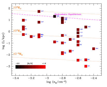
Figure 8: The line of sight thickness versus gas density as obtained from the PI models. Each data point is color-coded by the corresponding metallicity. The dashed line marks the relationship under local hydrostatic equilibrium (Schaye, 2001). High metallicity systems are too small to be self-gravitating. The dotted lines indicate the lines of constant masses. The majority of the systems contain gas masses of $\lesssim 10^{5}M_{\odot}$.

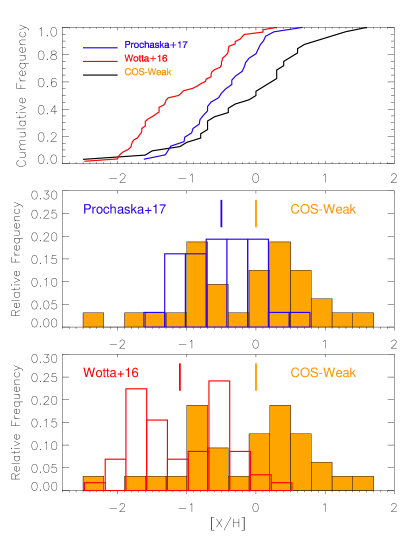
Figure 9: Bottom: Metallicity distribution of the weak absorbers in our sample (black histogram with orange shade). The red histogram in the bottom panel shows the bimodal metallicity distribution of H i-selected low-$z$ Lyman limit systems studied by Wotta et al. (2016). The blue histogram in the middle panel shows the metallicity distribution of the COS-Halos (galaxy-selected) sample from Prochaska et al. (2017). The top panel shows the cumulative distributions of all three sample with respective colors. Both the galaxy-selected and H i-selected absorbers show very different metallicity distributions when compared to the weak absorbers. Our sample shows the highest fraction ($\approx 50$%) of solar/super-solar metallicity absorbers.

Following Stocke et al. (2013), the number of metal-rich clouds inside the characteristic radius is $N_{cl}=C_{f}S(\frac{R_{h}}{R_{cl}})^{2}\approx 3\times 10^{5}$, assuming the “shadowing factor” ($S$) and $C_{f}$ to be of order unity. The volume filling factor of these clouds is then $N_{cl}(R_{cl}/R_{h})^{3}\approx 0.002$ (i.e. only $\approx 0.2$%). The total gas mass ($M_{\rm gas}=N_{cl}<M_{cl}>$) associated with these absorbers is $\sim 3\times 10^{8}$ $M_{\odot}$. This mass estimate is significantly lower compared to the COS-Halos sample (i.e., $>6\times 10^{10}$ $M_{\odot}$; Werk et al., 2014) but roughly matches with the calculation of Stocke et al. (2013) for their sample of dwarf galaxies. The mass in Silicon ($N_{cl}<M_{cl}>\rm<[Si/H]>(Si/H)_{\odot}$) is $\sim 10^{4}$ $M_{\odot}$. It corresponds to an Oxygen mass of $M_{O}\sim 10^{5}$ $M_{\odot}$, assuming solar relative abundance. This Oxygen mass estimate is $\approx 2$ orders of magnitude lower than the estimate of Tumlinson et al. (2011) for the O vi absorbing gas in the COS-Halos sample. Here we note that, all our mass estimates are lower limits in the sense that we do not take the possible contribution from the high-ionization gas phase into account.

From the discussion above, it is clear that the weak absorbers may stem from extended gaseous halos that are filled with large numbers of pc–kpc-scale clouds. Given the high metallicities of the majority of the weak absorbers, it is most natural to think that they arise in large scale galactic outflows. An important question in this context is the stability of the absorbing clouds. Self-gravity and external pressure due to an ambient medium are generally thought to be the two main channels that can confine the small, metal-rich clouds (see e.g. Schaye et al., 2007). The typical size for an optically thin, self-gravitating, purely gaseous cloud with density $\sim 10^{-2.8\pm 0.5}\rm cm^{-3}$ is $\sim$10–30 kpc (see Eqn. 7 in Schaye et al., 2007), whereas, the median line of sight thickness of our sample is $\approx 500$ pc. As demonstrated in Fig. 8, a vast majority of the weak absorbers in our sample are too tiny to be supported by self-gravity unless they are significantly dark matter dominated structures.

The presence of another gas phase, giving rise to the high-ionization metal lines, particularly the O vi, is almost certain (see Section 4.4). This phase, presumably with lower density and higher temperature, can, in principle, confine the low-ionization gas phase. However, in cases where detailed ionization modelling has been done the two phases are not found to be in pressure equilibrium (e.g. Meiring et al., 2013; Muzahid, 2014; Muzahid et al., 2015b; Hussain et al., 2015). But the high-ionization gas phase traced by O vi could arise from the mixing layers of cool and an ambient medium too hot for UV line diagnostics. This hotter unobserved gas, e.g., hot halo created via accretion shocks and/or shocks due to large-scale galactic outflows, might well be the confining medium (e.g., Mulchaey & Chen, 2009; Narayanan et al., 2011). Indeed, X-ray observations have revealed the presence of such a medium with $T>10^{6}$ K in the halo of Milky Way (Gupta et al., 2012). In the absence of any confining agent, the clouds will expand freely until they reach pressure equilibrium or will eventually be evaporated. For a $\sim 10^{4}$ K gas cloud with $R_{cl}\sim 10^{2}$ pc, the free expansion time scale is $R_{cl}/c_{s}\sim 10^{7}$ yr, much shorter than the Hubble time. This suggests that the high metallicity weak absorbers could be transient in nature.

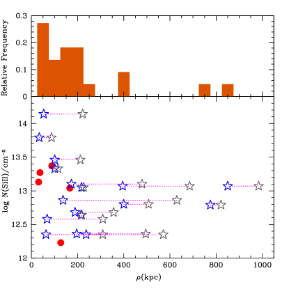
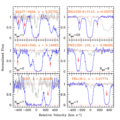
Figure 10: Left: The distribution of impact parameters of nearest known galaxies (top) for 22 of the weak absorbers. The impact parameter ranges from 31–850 kpc with a median value of 166 kpc. Only 3/22 absorbers show host-galaxy impact parameters $<50$ kpc. In 17/22 cases at least 2 galaxies are found within 1 Mpc from the QSO sightline and within a velocity window of $\pm$500 km s^-1 around the absorption redshift. In the bottom panel, the Si ii column densities are plotted against the impact parameters of the nearest galaxies (blue star) and the second nearest galaxies (grey star) connected by the dotted (magenta) line. The (red) filled circles represent the galaxies that do not have a known companion. No significant correlation is seen between $N(\mbox{Si\,{\sc ii}})$ and $\rho$. Right: The H i absorption profiles of 6 weak absorbers around which different number of galaxies ($N_{\rm gal}=$ 0–23) have been identified. No galaxy information is available for the system towards 3C57. The C ii absorption profiles are shown in grey. Note that all of them show additional H i absorption within $\pm$500 km s^-1 of the absorption redshift (0 km s^-1) indicated by the arrows. The presence of additional absorption clouds further suggests that they arise from a group environment (see text).

5.3 Metal Abundance

The most interesting physical properties of the weak absorbers is their unusual high metallicities. The median value of the $\rm[Si/H]$ distribution of $0.0$ indicates that $\approx$50% of the weak absorbers in our sample show a solar/super solar $\rm Si$ abundance. Moreover, 27/32 absorbers ($\approx 85$%) show $\rm[Si/H]>-1.0$. If we consider only $Q>2$ systems, then the fraction of absorbers showing $\rm[Si/H]\geq 0.0$ ($\geq-1.0$) is $\approx 44$% ($\approx 87$%). Here we note that the fraction of weak absorbers showing high metallicity is significantly higher compared to the H i-selected sample of Wotta et al. (2016) and the galaxy-selected sample of Prochaska et al. (2017). In Fig. 9 we compare the metallicity distributions of these three samples. The cumulative metallicity distribution, shown in the top panel, of our low-$z$ sample is significantly different compared to that of Wotta et al. (2016). A two-sided KS-test gives $D_{\rm KS}=0.51$ and $P_{\rm KS}=2.1\times 10^{-5}$ confirming that the difference has a 99.99% significance. The significance is somewhat lower ($\approx 98$%) with a $D_{\rm KS}=0.37$ when compared with the COS-Halos sample (Prochaska et al., 2017). The median metallicities of Wotta et al. (2016) and Prochaska et al. (2017) samples, i.e., $-1.1$ and $-0.5$ dex respectively, are much lower than our sample. Only 3/58 ($\approx$5%) of the absorbers in Wotta et al. (2016) and 7/31 ($\approx$22%) of the absorbers in Prochaska et al. (2017) have solar/super-solar metallicities. Clearly, the weak absorbers are significantly more metal-rich when compared to the galaxy-selected and H i-selected samples of absorbers probing the CGM at, by and large, similar redshifts .

Here we point out that both Wotta et al. (2016) and Prochaska et al. (2017) have used an UVB calculated by Haardt & Madau (2012, HM12 hereafter). The intensity of the HM12 UVB is somewhat lower than that of the KS15 UVB used in this study, for energies $>1$ Ryd (see e.g., Fig. 1 of Hussain et al., 2017). In order to assess the effect of the UVB on our metallicity estimates, we model an imaginary cloud at $z=0.1$ with column densities of H i, Si ii, and Si iii equal to the corresponding median values we obtained for our sample (i.e. $10^{16.0}$, $10^{12.9}$, and $10^{13.2}$ cm^-2, respectively). Grids of constant density cloudy models were run with a solar metallicity and with a stopping $N(\mbox{H\,{\sc i}})$ of $10^{16.0}$ cm^-2. The density derived for the HM12 UVB (i.e., $10^{-3.3}\rm cm^{-3}$) is $\approx 0.4$ dex lower than that obtained for the KS15 UVB. However, the metallicity obtained for the HM12 UVB (i.e., $\rm[Si/H]=-0.14$) is only $\approx 0.1$ dex lower than that derived for the KS15 UVB. Thus, overall, our metallicity estimates are consistent with those expected from the HM12 UVB.

Next, we evaluate the effect on the derived metallicity of the imaginary cloud, if some amount of Si iii is contributed by the high ionization gas phase, as it might be the case for some of the absorbers studied here. We found that even if 90% of the $N(\mbox{Si\,{\sc iii}})$ is contributed by the high ionization phase (i.e. using $\log N(\mbox{Si\,{\sc iii}})/\rm cm^{-2}$ of 12.2 instead of 13.2 in the model), the derived metallicity changes only by $\approx 0.1$ dex for both KS15 and HM12 incident continua. The density in such a situation is increases by $\approx 0.6$ dex, as expected.

In order to investigate whether the inferred abundances of $\rm[Si/H]>0.301$ ($>2$ times solar) for the 10 systems in our sample remain as high, we recalculate the metallicities and densities using a new cloudy grid with a super-solar metallicity of $\rm[X/H]=0.699$ (5 times solar). We find that the $\rm[Si/H]$ values are consistent within 0.2 dex. The densities, however, decrease by $\approx 0.6$ dex leading to an increase in $N_{\rm H}$ by 0.3 dex and in line-of-sight thickness by 0.9 dex. The decrease in density for the super-solar cloudy grid increases the column densities for the high-ions (i.e., C iv, N v, and O vi). Nonetheless, the predicted high-ions column densities, particularly the $N(\mbox{O\,{\sc vi}})$ and $N(\mbox{N\,{\sc v}})$, are still very low (e.g., $\log N/\rm cm^{-2}<13.5$). The predicted $N(\mbox{C\,{\sc iv}})$ values, although increased by 0.8–1.0 dex, are still consistent with the $3\sigma$ upper limits or are lower than the observed values except for the two systems ($z_{\rm abs}$ $=0.00575$ towards RXJ1230.8+0115 and $z_{\rm abs}$ $=0.09784$ towards SDSSJ1357+1704) as already noted in Section 4.4.

Finally, besides the absolute abundances, the measurements of $N(\mbox{C\,{\sc ii}})$ allow us to calculate the relative abundance of $\rm Si$ relative to $\rm C$, i.e., the $\rm[C/Si]$. We find $\rm[C/Si]=0.13\pm 0.18$(std), which is somewhat higher albeit consistent with solar value. Our estimates of $\rm[C/Si]$ are generally comparable to the $\rm[C/\alpha]$ measurements in solar-type stars in the Galactic disk (Gustafsson et al., 1999).

5.4 Galaxy Environments

[t] QSO $z_{\rm abs}$ Galaxy $z_{\rm gal}$ $\rho$(kpc) Comments/References PG0003+158 0.16512 SDSSJ000600.63+160908.1 0.16519 127 SDSS+ 2 Photo-z objects at 678 kpc and 876 kpc Q0107-025A 0.22722 17.56667,-2.32678 0.2272 166 Crighton et al. (2010) + 2 Photo-z objects at 170 kpc and 921 kpc HE0153-4520 0.22597 … … … Outside SDSS 3C57 0.32338 … … … Outside SDSS SDSSJ0212-0737 0.01603 SDSSJ021213.92-073500.9 0.017471 53 SDSS SDSSJ021202.56-074747.7 0.016501 222 SDSS SDSSJ021315.80-073942.6 0.015942 278 SDSS SDSSJ021323.81-074355.5 0.016087 340 SDSS SDSSJ021327.79-074150.0 0.016701 358 SDSS SDSSJ021529.88-071741.5 0.016032 994 SDSS SDSSJ0212-0737 0.13422 … … … 2 Photo-z objects at 796 kpc and 827 kpc UKS-0242-724 0.06376 … … … Outside SDSS Q0349-146 0.07256 … … … Outside SDSS PKS0405-123 0.16710 61.95084, -12.18361 0.1670 101 Prochaska et al. (2006) 61.83833, -12.19389 0.1670 115 Prochaska et al. (2006) IRAS-F04250-5718 0.00369 … … … Outside SDSS FBQS-0751+2919 0.20399 … … … … VV2006J0808+0514 0.02930 SDSSJ080839.55+051725.9 0.030795 101 SDSS SDSSJ080816.43+051258.0 0.030754 212 SDSS SDSSJ080901.35+051832.7 0.028036 227 SDSS SDSSJ080857.48+052138.0 0.030555 303 SDSS SDSSJ080758.11+051223.6 0.029165 360 SDSS SDSSJ081009.39+051749.6 0.028946 783 SDSS SDSSJ080811.31+053514.4 0.030753 790 SDSS PG0832+251 0.02811 SDSSJ083720.73+245627.2 0.027126 775 SDSS SDSSJ083720.63+250915.8 0.026954 821 SDSS SDSSJ083726.34+250338.8 0.028623 862 SDSS SDSSJ083736.98+245959.1 0.028897 943 SDSS SDSSJ0929+4644 0.06498 SDSSJ092855.37+464345.9 0.065031 189 SDSS SDSSJ092849.63+464057.5 0.064019 356 SDSS SDSSJ092849.95+463912.0 0.064096 454 SDSS SDSSJ092841.92+463841.5 0.064556 548 SDSS PMNJ1103-2329 0.08352 … … … Outside SDSS PG1116+215 0.13850 169.77779, 21.30785 0.13814 137 Tripp et al. (1998), SDSS 169.77117, 21.25083 0.13736 630 Tripp et al. (1998) 169.70834, 21.26972 0.13845 776 Tripp et al. (1998) SDSSJ1122+5755 0.05319 SDSSJ112225.88+580147.3 0.052616 400 SDSS SDSSJ112248.77+580358.3 0.053144 507 SDSS SDSSJ112359.26+575248.2 0.052292 622 SDSS SDSSJ112227.55+580614.2 0.053132 661 SDSS SDSSJ112207.40+580604.3 0.052983 703 SDSS PG1121+422 0.19238 SDSS J112428.67+420543.8 0.193994 850 SDSS SDSS J112445.06+415641.9 0.192222 984 SDSS 3C263 0.06350 175.02154, 65.80042 0.06322 63 Savage et al. (2012) 174.73408, 65.87654 0.06281 571 Savage et al. (2012) 174.74136, 65.88236 0.06285 576 Savage et al. (2012) 175.52030, 65.81338 0.06498 956 Savage et al. (2012) PG1202+281 0.13988 … … … 1 Photo-z object at 912 kpc PG-1206+459 0.21439 NA 0.2144 31 Rosenwasser et. al, Submitted SDSSJ1210+3157 0.05974 SDSS J121028.01+315838.1 0.059548 173 SDSS SDSS J121012.30+320137.3 0.059628 479 SDSS SDSS J121004.05+320115.2 0.060117 567 SDSS SDSS J120957.35+320024.6 0.058957 619 SDSS SDSS J121013.63+320501.4 0.060975 657 SDSS SDSS J121015.27+320854.7 0.059088 862 SDSS SDSS J120942.22+320258.8 0.058983 888 SDSS SDSSJ1210+3157 0.14964 … … … 1 Photo-z object at 832 kpc SDSSJ1214+0825 0.07407 SDSSJ121425.17+082251.8 0.073271 217 SDSS SDSSJ121431.23+082225.6 0.074042 226 SDSS SDSSJ121428.14+082225.5 0.072431 227 SDSS SDSSJ121439.76+082157.4 0.073442 324 SDSS SDSSJ121511.53+082444.3 0.073495 842 SDSS SDSSJ121511.14+082556.7 0.073064 831 SDSS

Table 4: List of galaxies around weak absorbers.

[t] QSO $z_{\rm abs}$ Galaxy $z_{\rm gal}$ $\rho$(kpc) Comments/References RXJ1230.8+0115 0.00575 SDSSJ123246.60+013408.1 0.005088 215 SDSS SDSSJ123246.10+013407.8 0.005166 218 SDSS SDSSJ123320.76+013117.7 0.005557 227 SDSS SDSSJ122950.57+020153.7 0.005924 353 SDSS SDSSJ123227.94+002326.2 0.005051 354 SDSS SDSSJ123013.38+023730.5 0.00544 549 SDSS SDSSJ123014.49+023717.6 0.005494 553 SDSS SDSSJ123821.70+011207.5 0.004152 574 SDSS SDSSJ122902.17+024323.8 0.005221 587 SDSS SDSSJ123422.01+021931.4 0.005871 596 SDSS SDSSJ123238.38+024015.6 0.005692 619 SDSS SDSSJ123236.14+023932.5 0.005867 632 SDSS SDSSJ123251.28+023741.6 0.005911 633 SDSS SDSSJ122803.19+025449.7 0.004871 642 SDSS SDSSJ122658.50+022939.4 0.005645 649 SDSS SDSSJ122803.67+025434.9 0.004994 657 SDSS SDSSJ123434.98+023407.7 0.006155 727 SDSS SDSSJ123902.48+005058.9 0.005316 815 SDSS SDSSJ123805.17+012839.9 0.006158 832 SDSS SDSSJ123642.07+030630.3 0.004861 842 SDSS SDSSJ122329.97+020029.0 0.006051 878 SDSS SDSSJ122815.88+024202.9 0.007397 885 SDSS SDSSJ122323.40+014854.1 0.006295 895 SDSS PKS1302-102 0.09495 196.38375, -10.56555 0.09358 68 Cooksey et al. (2008) 196.34417, -10.58000 0.09328 309 Cooksey et al. (2008) 196.33708, -10.58083 0.09393 350 Cooksey et al. (2008) 196.34874, -10.50694 0.09331 386 Cooksey et al. (2008) 196.30041, -10.57250 0.09531 548 Cooksey et al. (2008) 196.28833, -10.61417 0.09523 715 Cooksey et al. (2008) 196.31500, -10.46389 0.09442 728 Cooksey et al. (2008) 196.42292, -10.44000 0.09332 756 Cooksey et al. (2008) 196.36833, -10.42083 0.09402 852 Cooksey et al. (2008) SDSSJ1322+4645 0.21451 NA 0.2142 37 Werk et al. (2014) + 2 Photo-z objects at 395 kpc and 821 kpc SDSSJ1357+1704 0.09784 … … … 2 Photo-z objects at 303 kpc and 491 kpc SDSSJ1419+4207 0.17885 NA 0.1792 88 Werk et al. (2014) PG1424+240 0.12126 SDSSJ142701.72+234630.9 0.121177 196 SDSS SDSSJ142714.52+235007.4 0.119514 495 SDSS PG1424+240 0.14683 … … … 2 Photo-z objects at 940 kpc and 950 kpc PG-1630+377 0.17388 SDSSJ163155.09+373556.5 0.175373 395 SDSS SDSSJ163149.79+373438.7 0.17391 685 SDSS PHL1811 0.07774 J215450.8-092235 0.078822 237 Keeney et al. (2017) J215447.5-092254 0.077671 309 Keeney et al. (2017) SDSSJ215506.02-091627.0 0.078655 526 SDSS SDSSJ215453.14-091559.2 0.077813 584 SDSS SDSSJ215434.62-091632.7 0.078369 766 SDSS SDSSJ215536.27-092017.7 0.077963 766 SDSS SDSSJ215437.22-091534.4 0.078117 787 SDSS PHL1811 0.08091 J21545996-0922249 0.0808 34 Jenkins et al. (2005) J21545870-0923061 0.0804 87 Jenkins et al. (2005)

Table 4: Cont.

Notes– The impact parameters from the literature are corrected for the adopted cosmology.

In what types of galaxy environments do the low-$z$ weak absorbers reside? In order to investigate, we have searched for galaxies around these absorbers in SDSS and in the literature. We have found host-galaxy information for 22/34 absorbers. In our SDSS search we have queried for galaxies with spectroscopic redshifts consistent within $\pm 500$ km s^-1 of $z_{\rm abs}$ and within 1 Mpc projected separation from the QSO sightline. The SDSS spectroscopic database is 90% complete down to an $r$-band apparent magnitude, $m_{r}$, of 17.77 (Strauss et al., 2002; Blanton et al., 2003a). This corresponds to a luminosity of $>1.2L_{*}$ at $z=0.1$ (Blanton et al., 2003b, no K-correction has been applied). The details of the galaxies around the weak absorbers are listed in Table 4. In the left panel of Fig. 10 we show the impact parameter distribution of the nearest known galaxies which varies from 31–850 kpc. Interestingly, the median impact parameter of 166 kpc is in agreement with the halo radius ($R_{h}$) we estimated in Section 5.2. Albeit having high metallicities, only $\approx 14$% (3/22) of the absorbers have nearest known bright galaxies within 50 kpc. However, for $\approx 70$% of the cases a galaxy is detected within 200 kpc. We did not find any trend between $N(\mbox{Si\,{\sc ii}})$, metallicity (or density) and the impact parameter of the nearest known galaxy.

There are 26/34 fields that are covered in the SDSS footprint. We have found 75 galaxies in total in these fields ($<1$ Mpc) around the weak absorbers ($\pm 500$ km s^-1) in contrast to only 6 galaxies detected in random 26 fields. It indicates a significant galaxy-overdensity around the low-$z$ weak absorbers. Furthermore, in about $\approx 80$% (17/22) of the cases we find 2 or more galaxies within 1 Mpc from the sightline and within a velocity window of $\pm 500$ km s^-1 (see Table 4). All these facts suggest that the majority of the weak absorbers live in galaxy groups. Interestingly, as many as 23 galaxies are found around the absorber at $z_{\rm abs}$ $=0.00575$ towards RXJ1230.8+0115, in which the sightline passes through the Virgo cluster (Yoon & Putman, 2017). In 6/26 cases the SDSS search did not yield even one galaxy that satisfied our criteria. Nonetheless, galaxies with consistent photometric redshifts are identified in all but one case. A detail study of all the galaxies listed in Table 4 will be presented in future.

If a line of sight passes through multiple galaxy halos in a group, then it is more likely to observe more than one absorption clump within the characteristic group velocity. We, thus, re-examine the $\pm 500$ km s^-1 velocity range around the Ly$\alpha$ absorption in each of the weak absorbers to investigate any such possible signs of group environment. The total redshift path-length covered by this velocity range is $\approx 0.127$. From the observed $d\mathcal{N}/dz$ (Danforth et al., 2016), the expected number of random IGM H i clouds with $N(\mbox{H\,{\sc i}})>10^{13.5}$ at $z\approx 0.1$ is 24. Intriguingly, we have found nearly 60 H i absorbers (including the 34 weak absorbers) which is $\approx 2.5$ times higher than the number expected from random chance coincidence. As an example, the $\pm 500$ km s^-1 spectral ranges for 6 of the weak absorbers are shown in the right panel of Fig. 10. For all of the 6 cases additional H i absorption has been detected, even when no galaxies have been identified or known in the field. It possibly suggests that all of these weak absorbers may reside in group environments even if the group environment is not apparent from the existing galaxy data. We recall here that the SDSS spectroscopic database is sensitive only to bright ($>1.2L_{*}$) galaxies. A systematic survey of galaxies around these fields is thus essential.

Alternatively, or in addition, a group environment may be conducive to processes that give rise to these high metallicity clouds far from galaxy centers. A clue about the processes at work in galaxy groups is provided by the study of O vi absorbers by Pointon et al. (2017). They find that O vi is weaker and has a narrower velocity distribution for lines of sight through groups than for those near isolated galaxies. They interpret this to mean that a group is heated beyond the point where individual O vi halos would be superimposed to produce stronger absorption. They suggest that the O vi that is observed is at the interface between the hot, X-ray gas and the cooler CGM. Weak, low-ionization absorption could also be related to such an interface via thermal/hydrodynamical instabilities.

5.5 Possible Origin(s)

The high metallicity ($\rm[Si/H]\approx 0.0$) and solar relative abundances of heavy elements ($\rm[C/Si]\approx 0.13\pm 0.18$) strongly suggest that the absorbing clouds are related to star-forming regions. The impact parameters of the nearest galaxies of $>50$ kpc imply that mechanisms such as galactic/AGN winds and/or tidal/ram pressure stripping of the ISM of satellite galaxies at early epochs could give rise to the cool clouds seen in absorption. Recall that the majority of the weak absorbers seems to live in a group environment in which interactions are common, and gas is often stripped from individual galaxies.

The metal-enriched, cool clouds can form in outflows predominantly via two different channels. First, metal-rich ISM clouds can be swept-up by hot wind material to the CGM by means of ram pressure and radiation pressure (e.g., Zubovas & Nayakshin, 2014; McCourt et al., 2015; Schneider & Robertson, 2017; Heckman et al., 2017). Second, the clouds can form in-situ, condensing out of the hot wind due to thermal instabilities (e.g., Field, 1965; Costa et al., 2015; Voit et al., 2016; Ferrara & Scannapieco, 2016; Thompson et al., 2016). Recently, McCourt et al. (2016) have suggested that an optically thin, $T\sim 10^{6}$ K cooling perturbation with an initial size $\gg c_{s}t_{\rm cool}$ ($c_{s}$ is the internal sound speed, $t_{\rm cool}$ is the cooling time) will be fragmented quickly to a large number of cloudlets due a process called “shattering”, giving rise to a “fog” like structure. These fragments are found to have a characteristic length-scale of $l_{\rm cloudlet}\sim 0.1\rm pc\leavevmode\nobreak\ (n_{\rm H}/\rm cm^{-3})^{-1}$ as they reach a temperature of $\sim 10^{4}$ K. The column density of an individual cloudlet is then $N_{\rm cloudlet}=n_{\rm H}l_{\rm cloudlet}\sim 10^{17.5}$ cm^-2. It is interesting to note that the median $N_{\rm H}$ of our sample, $\approx 10^{18.1}$ cm^-2, is broadly in agreement with their prediction. Here we also recall that a large number of such clouds is indeed required to match the observed $d\mathcal{N}/dz$ (see Section 5.2). These facts indicate that the “fog” like structure as suggested by McCourt et al. (2016) is consistent with the properties of the weak absorbers.

In both the situations discussed above the clouds will be metal-rich but will be subject to hydrodynamical (e.g., Rayleigh–Taylor, Kelvin–Helmholtz) instabilities (Klein et al., 1994). Moreover, cloud-wind interactions will also disrupt/shred the clouds on a “crushing” time-scale which is roughly similar to the time-scales of hydrodynamical instabilities. Radiative cooling and the presence of magnetic field can extend the lifetime of the cloud considerably (e.g., Cooper et al., 2009; McCourt et al., 2015). Next generation cosmological hydrodynamical simulations that can resolve pc-scale structures are essential for better theoretical understanding of the origins of these exciting absorbers.

6 summary

Using archival $HST/$COS spectra we have conducted a survey (“COS-Weak”) of low-ionization weak metal line absorbers, with $W_{r}(\mbox{C\,{\sc ii}}\lambda 1334)<0.3$ Å and $W_{r}(\mbox{Si\,{\sc ii}}\lambda 1260)<0.2$ Å at $z<0.3$, that are analogous to weak Mg ii absorbers which are mostly studied at high-$z$. We have constructed the largest sample of weak absorber analogs that comprises of 34 absorbers, increasing the number of known/reported weak absorbers by a factor of $>5$ at low-$z$. We have measured column densities of low- and high-ionization metal lines and of H i, performed simple photoionization models using cloudy, and have discussed the implications of the observed and inferred properties of these absorbers and their galaxy environments. Our main findings are as follows:

• We estimate $d\mathcal{N}/dz=0.8\pm 0.2$ for our survey at $z<0.3$, consistent with the previous study of Narayanan et al. (2005). This implies that the processes that produce the weak absorber clouds are less active at low-$z$ than at $z\approx 1$ (Section 3.1 & 5.1).

• Our simple photoionization models assumed Si iii and Si ii arise in the same phase, and that most/all of the H i absorption is also in this phase. Absorber densities range from $10^{-3.3}$ to $10^{-2.4}$ cm^-3, with a median of $10^{-2.8}$ cm^-3. Metallicities, represented as $\rm[Si/H]$, ranged from $-2.5$ to $1.6$, with a median of $0.0$. The line of sight thicknesses of the clouds ranged from 1 pc to 53 kpc. The neutral hydrogen column densities range from $\log N(\mbox{H\,{\sc i}})/\rm cm^{-2}$ of 14–18, and the total hydrogen column densities $\log N_{\rm H}/\rm cm^{-2}$ from 16–20. There is an anti-correlation between $\rm[Si/H]$ and $N(\mbox{H\,{\sc i}})$. Although this is partly a selection effect for small $N(\mbox{H\,{\sc i}})$, it is clear that the highest metallicities do arise in environments that do not have a large amount of neutral hydrogen nearby to dilute the metals (Fig. 7).

• At least two thirds of the absorbers have a separate, hotter and/or higher ionization phase with C iv and/or O vi absorption detected. In several cases C iv can arise in the same phase with the Si ii/C ii, but generally when it is detected a separate phase is needed. O vi must always arise in a different phase (Section 4.4).

• We find that the highest metallicity systems are the tiniest in size (Fig. 8). The majority of these absorbers have (gas) masses ($<10^{5}M_{\odot}$) too small to be in local hydrostatic equilibrium unless they are significantly dark matter dominated structures. In the absence of any confining medium these absorbers will be evaporated on the free expansion time-scale of $\sim 10^{7}$ yr.

• The weak absorbers outnumber bright galaxies by tens of thousands in one, suggesting that the population must be huge. Nonetheless, they carry a negligible fraction of cosmic baryons. Adopting the geometrical model for CGM absorbers prescribed by Richter et al. (2016a), we obtain a covering fraction of $\approx$30% for the weak absorbers, assuming that the population extends out to the virial radii of galaxies with $L/L_{*}>0.001$ (Section 5.2).

• The weak absorber population is found to be significantly more metal-rich compared to the H i-selected (Wotta et al., 2016) and galaxy-selected (Prochaska et al., 2017) samples of absorbers probing the CGM at similar redshift (Section 5.3).

• We have searched for galaxies around these absorbers in SDSS and in the literature and found that they live in regions of significant galaxy over-density. In about 80% of the cases, more than one galaxy is detected within 1 Mpc from the QSO sightline and within $\pm 500$ km s^-1 of the absorber’s redshift. The impact parameters of the nearest known galaxies range from $\approx$31–850 kpc with a median of 166 kpc. In $\approx$70% of the cases the nearest galaxy is detected within 200 kpc. It implies that the weak absorbers are abundant in the halos of galaxies that are in group environments (Section 5.4).

  The origin of these metal-rich, compact structures, apart from galaxies, remains unclear, but we suggest that they are transient structures in the halos of galaxies most of which live in group environments and they are related to outflows and/or to stripping of metal-rich gas from the galaxies. A systematic search for galaxies in these fields and next generation cosmological simulations with the capability of resolving pc-scale structures are essential for further insights into the nature and origin of these fascinating cosmic structures.

Acknowledgements: Support for this research was provided by NASA through grants HST AR-12644 from the Space Telescope Science Institute, which is operated by the Association of Universities for Research in Astronomy, Inc., under NASA contract NAS5-26555. SM thanks Tiago Costa for stimulating discussion on the theoretical aspects of galaxy outflows. SM thankfully acknowledges IUCAA (India) for providing hospitality while a part of the work was done. SM also acknowledges support from the European Research Council (ERC), Grant Agreement 278594-GasAroundGalaxies. This work is benefited from the SDSS. Funding for the Sloan Digital Sky Survey IV has been provided by the Alfred P. Sloan Foundation, the U.S. Department of Energy Office of Science, and the Participating Institutions. SDSS-IV acknowledges support and resources from the Center for High-Performance Computing at the University of Utah. The SDSS web site is www.sdss.org.

SDSS-IV is managed by the Astrophysical Research Consortium for the Participating Institutions of the SDSS Collaboration including the Brazilian Participation Group, the Carnegie Institution for Science, Carnegie Mellon University, the Chilean Participation Group, the French Participation Group, Harvard-Smithsonian Center for Astrophysics, Instituto de Astrofísica de Canarias, The Johns Hopkins University, Kavli Institute for the Physics and Mathematics of the Universe (IPMU) / University of Tokyo, Lawrence Berkeley National Laboratory, Leibniz Institut für Astrophysik Potsdam (AIP), Max-Planck-Institut für Astronomie (MPIA Heidelberg), Max-Planck-Institut für Astrophysik (MPA Garching), Max-Planck-Institut für Extraterrestrische Physik (MPE), National Astronomical Observatories of China, New Mexico State University, New York University, University of Notre Dame, Observatário Nacional / MCTI, The Ohio State University, Pennsylvania State University, Shanghai Astronomical Observatory, United Kingdom Participation Group, Universidad Nacional Autónoma de México, University of Arizona, University of Colorado Boulder, University of Oxford, University of Portsmouth, University of Utah, University of Virginia, University of Washington, University of Wisconsin, Vanderbilt University, and Yale University.

Appendix A Connection to weak Mg ii absorbers

In this Appendix we revisit the connection between Si ii and Mg ii absorption and confirm that our selection criteria are indeed well suited for studying the weak Mg ii absorbers at $z<0.3$ in the absence of spectral coverage for the Mg ii doublet.

In Section 1, we have argued that Si ii is a good proxy for Mg ii. The top panel of Fig. 11 further strengthens our argument. For typical $N(\mbox{H\,{\sc i}})$ and $\rm[X/H]$ it shows that Si ii traces Mg ii for a wide range of densities relevant for these absorbers. In the bottom panel, the $N(\mbox{Mg\,{\sc ii}})$ values predicted by our adopted PI models are plotted against the observed $N(\mbox{Si\,{\sc ii}})$. As expected, a statistically significant correlation is seen between these two quantities. The predicted $N(\mbox{Mg\,{\sc ii}})$ values are in the range of $10^{11.6-13.8}$ cm^-2 with a median of $10^{12.3}$ cm^-2. An equivalent width of 0.3 Å corresponds to a column density of $10^{12.84}$ cm^-2 (indicated by the red horizontal line) for the Mg ii$\lambda 2796$ line on the linear part of the COG. A vast majority (28/32) of the systems show $N(\mbox{Mg\,{\sc ii}})<12.84$, indicating that these are truly analogous to the weak Mg ii absorbers that are primarily studied at high-$z$.

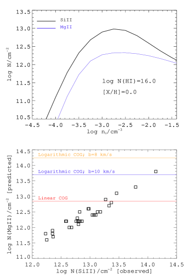
Figure 11: Top: cloudy predicted column densities of Si ii (black) and Mg ii (blue) as a function of density. The model is run with a stopping $N(\mbox{H\,{\sc i}})$ of $10^{16}$ cm^-2 and with a solar metallicity. Si ii and Mg ii closely follow each other for a wide range in density. Bottom: The model predicted Mg ii column densities, listed in the last column of Table 2, against the observed Si ii column densities. As expected from the top panel, a tight correlation ($\rho_{s}=0.92,\rho_{s}/\sigma=5.2$) between $N(\mbox{Mg\,{\sc ii}})$ and $N(\mbox{Si\,{\sc ii}})$ is seen. The horizontal lines correspond to the maximum $N(\mbox{Mg\,{\sc ii}})$ for an weak Mg ii absorber with $W_{r}(\mbox{Mg\,{\sc ii}}\lambda 2796)<0.3$ Å, provided the line falls on the linear part of the COG or logarithmic part of the COG with $b=$ 10 and 8 km s^-1. Clearly, all of these absorbers are consistent with being weak Mg ii absorbers’ analogs.

Appendix B Supplementary Lists

Table 1: List of QSO spectra with $\rm S/N>5$ per pixel searched for weak Mg ii analogs. The full list is available as “online only” material.

QSO	RA	Dec	$z_{\rm qso}$	Gratings	$z_{\rm min}$	$z_{\rm max}$	$(\rm S/N)_{G130M}$	$(\rm S/N)_{G160M}$	Flag	PID
(1)	(2)	(3)	(4)	(5)	(6)	(7)	(8)	(9)	(10)	(11)
PHL2525	0.10167	-12.76333	0.199	3	0.000	0.179	12	8	1	12604
PG0003+158	1.49683	16.16361	0.451	3	0.000	0.343	15	9	1	12038
MRK335	1.58125	20.20278	0.025	3	0.000	0.008	16	11	1	11524
SDSSJ0012-1022	3.10004	-10.37403	0.228	3	0.000	0.208	5	3	0	12248
QSO-B0026+129	7.30712	13.26778	0.142	1	0.000	0.086	11	-1	1	12569
HS-0033+4300	9.09575	43.27786	0.120	3	0.025	0.101	6	6	1	11632
SDSSJ0042-1037	10.59287	-10.62883	0.424	3	0.000	0.343	6	5	0	11598
PG0044+030	11.77458	3.33194	0.623	1	0.000	0.099	6	-1	1	12275
IO-AND	12.07908	39.68656	0.134	3	0.025	0.115	8	7	1	11632
QSO-B0050+124	13.39567	12.69331	0.059	1	0.000	0.040	10	-1	1	12569
HE0056-3622	14.65567	-36.10133	0.164	3	0.000	0.145	17	13	1	12604
RBS144	15.11296	-51.23172	0.062	3	0.000	0.044	13	10	1	12604
J0101+4229	15.37971	42.49322	0.190	3	0.025	0.170	6	5	1	11632
Q0107-025A	17.55475	-2.33136	0.960	3	0.000	0.347	10	12	1	11585
Q0107-0232	17.56012	-2.28267	0.728	2	0.135	0.349	-1	10	1	11585
Q0107-025B	17.56771	-2.31417	0.956	3	0.000	0.346	9	11	1	11585
B0117-2837	19.89871	-28.35872	0.349	3	0.000	0.345	15	17	1	12204
TONS210	20.46463	-28.34939	0.116	3	0.000	0.097	28	18	1	12204
B0120-28	20.65317	-28.72258	0.436	3	0.086	0.342	12	8	1	12204
FAIRALL9	20.94071	-58.80578	0.047	3	0.000	0.030	27	26	1	12604

Table 2: List of QSO spectra with $\rm S/N<5$ per pixel that are not used in this study. The full list is available as “online only” material.

QSO	RA	Dec	$z_{\rm qso}$	Gratings	$z_{\rm min}$	$z_{\rm max}$	$(\rm S/N)_{G130M}$	$(\rm S/N)_{G160M}$	Fl ag	PID
(1)	(2)	(3)	(4)	(5)	(6)	(7)	(8)	(9)	(10)	(11)
QSO-B0007+107	2.62925	10.97486	0.089	1	0.000	0.071	2	-1	1	12569
SDSSJ0242-0759	40.71188	-7.98728	0.172	3	0.000	0.152	4	4	0	12248
SDSSJ0843+4117	130.95620	41.29489	0.990	3	0.000	0.330	3	3	0	12248
VV2006J0852+0313	133.24675	3.22239	0.297	1	0.000	0.099	4	-1	0	12603
J0904P4007	136.09713	40.11797	0.411	2	0.108	0.323	-1	4	1	13423
SDSSJ0910+1014	137.62396	10.23711	0.463	3	0.000	0.345	4	4	0	11598
SDSSJ0912+2957	138.14758	29.95706	0.305	3	0.000	0.283	4	3	0	12248
VV2006J0914+0837	138.63238	8.62853	0.648	1	0.000	0.100	4	-1	0	12603
SDSSJ0930+2848	142.50791	28.81622	0.487	1	0.000	0.102	3	-1	0	12603
SDSSJ0935+0204	143.82578	2.07097	0.650	3	0.000	0.345	4	3	0	11598
VV2000J0936+3207	144.01617	32.11925	1.150	1	0.000	0.097	2	-1	0	12603
SDSSJ0937+1700	144.27854	17.00597	0.506	1	0.000	0.098	4	-1	0	12603
SDSSJ0943+0531	145.88170	5.52539	0.564	3	0.000	0.344	4	4	0	11598
SDSSJ0951+3307	147.78800	33.12939	0.644	1	0.000	0.102	3	-1	1	12486
BZBJ1001+2911	150.29254	29.19375	0.558	3	0.000	0.324	3	3	1	13008
VV96J1002+3240	150.72713	32.67753	0.829	1	0.000	0.100	3	-1	0	12603
2MASXJ1005-2417	151.38628	-24.28781	0.154	3	0.000	0.135	3	2	0	13347
J1010P2559	152.62725	25.99706	0.512	2	0.108	0.319	-1	4	1	13423
2MASSJ1013+0500	153.32487	5.00950	0.266	1	0.000	0.101	3	-1	0	12603
2MASSJ1015-2748	153.99683	-27.80800	0.102	3	0.000	0.084	4	2	0	13347

[t] QSO RA Dec $z_{\rm qso}$ $z_{\rm abs}$ Gratings $z_{\rm min}$ $z_{\rm max}$ $(\rm S/N)_{G130M}$ $(\rm S/N)_{G160M}$ Flag PID (1) (2) (3) (4) (5) (6) (7) (8) (9) (10) (11) (12) SDSSJ0012-1022 3.10004 -10.37403 0.228 0.22936 3 0.000 0.208 5 3 0 12248 SDSSJ0042-1037 10.59287 -10.62883 0.424 0.09487 3 0.000 0.343 6 5 0 11598 B0120-28 20.65317 -28.72258 0.436 0.18538 3 0.086 0.342 12 8 1 12204 PHL1226 28.61662 4.80519 0.404 0.01795 1 0.000 0.101 8 -1 1 12536 SDSSJ0155-0857 28.87509 -8.95111 0.165 0.16412 3 0.000 0.146 6 5 0 12248 VV2006J0159+1345 29.97067 13.76511 0.503 0.04419 1 0.000 0.100 6 -1 0 12603 Q0244-303 41.70779 -30.12814 0.530 0.00461 1 0.000 0.099 5 -1 1 12988 PG0832+251 128.89917 24.99472 0.329 0.01750 3 0.000 0.307 7 8 1 12025 Q0850+440 133.39266 43.81730 0.515 0.16368 3 0.000 0.329 13 6 0 13398 SDSSJ0925+4004 141.47793 40.07058 0.471 0.24766 3 0.000 0.344 4 5 0 11598 SDSSJ0928+6025 142.15824 60.42250 0.295 0.15384 3 0.000 0.273 4 5 0 11598 SDSSJ0930+2848 142.50791 28.81622 0.487 0.02284 1 0.000 0.102 3 -1 0 12603 SDSSJ0950+4831 147.50304 48.52481 0.589 0.21168 3 0.000 0.345 7 5 0 11598 SDSSJ0951+3307 147.78800 33.12939 0.644 0.00534 1 0.000 0.102 3 -1 1 12486 2MASSJ0951+3542 147.84971 35.71361 0.398 0.04435 1 0.009 0.103 7 -1 0 12603 SDSSJ0959+0503 149.81521 5.06531 0.162 0.05888 3 0.000 0.143 6 5 0 12248 SDSSJ1001+5944 150.26062 59.73730 0.746 0.30358 3 0.000 0.345 10 5 0 12248 SDSSJ1009+0713 152.25858 7.22883 0.456 0.11398 3 0.000 0.345 5 5 0 11598 J1010P2559 152.62725 25.99706 0.512 0.24464 2 0.108 0.319 -1 4 1 13423 SDSSJ1016+4706 154.09417 47.11203 0.821 0.16582 3 0.000 0.345 5 5 0 11598 SDSSJ1016+4706 154.09417 47.11203 0.821 0.25257 3 0.000 0.345 5 5 0 11598 Q1022+393 155.65591 39.53069 0.603 0.25225 2 0.121 0.328 4 -1 0 12593 SDSSJ1047+1304 161.79096 13.08183 0.400 0.00279 1 0.000 0.079 4 -1 1 12198 SDSSJ1112+3539 168.16296 35.65783 0.653 0.02480 3 0.000 0.345 4 4 0 11598 SDSSJ1117+2634 169.47630 26.57128 0.421 0.04747 3 0.000 0.326 6 5 0 12248 VV2006J1120+0413 170.02078 4.22314 0.544 0.04993 1 0.000 0.101 5 -1 0 12603 SDSSJ1133+0327 173.36576 3.45531 0.524 0.23733 3 0.000 0.345 5 3 0 11598 PG1216+069 184.83720 6.64403 0.331 0.00634 3 0.000 0.309 14 7 1 12025 SDSSJ1233+4758 188.39613 47.96678 0.381 0.22193 3 0.000 0.344 8 4 0 11598 SDSSJ1241+2852 190.37350 28.87000 0.589 0.06667 1 0.000 0.098 5 -1 0 12603 SDSSJ1241+5721 190.47508 57.35203 0.583 0.20558 3 0.000 0.345 7 6 0 11598/13033 VV2006J1305+0357 196.35108 3.95858 0.545 0.00144 1 0.000 0.101 7 -1 0 12603 CSO-0873 199.98433 27.46894 1.015 0.28899 2 0.252 0.329 10 -1 0 11667 SDSSJ1330+2813 202.68813 28.22261 0.417 0.19227 3 0.000 0.345 6 5 0 11598 SDSSJ1342+0505 205.52733 5.08994 0.266 0.13943 3 0.000 0.245 7 5 0 12248 SDSSJ1342-0053 205.71500 0.89592 0.326 0.07133 3 0.000 0.304 7 6 0 11598 SDSSJ1342-0053 205.71500 0.89592 0.326 0.22745 3 0.000 0.304 7 6 0 11598 SDSSJ1407+5507 211.88437 55.12378 1.026 0.00477 1 0.000 0.101 8 -1 1 12486 SDSSJ1410+2304 212.66001 23.07978 0.795 0.20962 3 0.000 0.340 7 6 1 12958 QSO-B1411+4414 213.45137 44.00389 0.089 0.08286 1 0.000 0.071 13 -1 1 12569 SDSSJ1415+1634 213.92876 16.57050 0.742 0.00770 1 0.000 0.085 10 -1 1 12486 SDSSJ1435+3604 218.79803 36.07700 0.428 0.20267 3 0.000 0.345 5 3 0 11598 SDSSJ1512+0128 228.15438 1.47944 0.265 0.02938 1 0.000 0.100 3 -1 0 12603 SDSSJ1553+3548 238.27050 35.80795 0.721 0.08292 3 0.000 0.344 7 4 0 11598 SDSSJ1555+3628 238.76830 36.48000 0.714 0.18915 3 0.000 0.345 5 3 0 11598 SDSSJ1616+4154 244.20590 41.90453 0.440 0.32098 3 0.077 0.345 6 5 0 11598 SDSSJ1619+3342 244.81894 33.71067 0.470 0.09638 3 0.000 0.345 10 10 0 11598 IRAS-F22456-5125 342.17165 -51.16475 0.100 0.09937 3 0.000 0.082 32 16 1 11686

Table 3: List of strong C ii$/$Si ii systems. These systems are not part of the sample studied here.

• Notes– (1) QSO name; (2) Right-ascension (J2000); (3) Declination (J2000); (4) QSO redshift; (5) Absorption redshift; (6) COS gratings used for observations, 1: G130M, 2: G160M, 3: G130M+160M; (7) Minimum search redshift; (8) Maximum search redshift; (9) S$/$N of the G130M data estimated near 1400 Å; (10) S$/$N of the G160M data estimated near 1600 Å. S$/$N is $-1$ when data are not available; (11) Spectrum flag, 1: part of the statistical sample, 0: not part of the statistical sample; (12) $HST$ proposal ID.

[t] QSO RA Dec $z_{\rm qso}$ $z_{\rm abs}$ Gratings $z_{\rm min}$ $z_{\rm max}$ $(\rm S/N)_{G130M}$ $(\rm S/N)_{G160M}$ Flag PID (1) (2) (3) (4) (5) (6) (7) (8) (9) (10) (11) (12) SDSSJ0012-1022 3.10004 -10.37403 0.228 0.22936 3 0.000 0.208 5 3 0 12248 SDSSJ0155-0857 28.87509 -8.95111 0.165 0.16412 3 0.000 0.146 6 5 0 12248 QSO-B1411+4414 213.45137 44.00389 0.089 0.08286 1 0.000 0.071 13 – 1 12569 IRAS-F22456-5125 342.17165 -51.16475 0.100 0.09937, 0.09592 3 0.000 0.082 32 16 1 11686

Table 4: List of weak Mg ii analogs that are intrinsic to the background QSO. These systems are not part of the sample studied here.

• Notes– (1) QSO name; (2) Right-ascension (J2000); (3) Declination (J2000); (4) QSO redshift; (5) Absorption redshift; (6) COS gratings used for observations, 1: G130M, 2: G160M, 3: G130M+160M; (7) Minimum search redshift; (8) Maximum search redshift; (9) S$/$N of the G130M data estimated near 1400 Å; (10) S$/$N of the G160M data estimated near 1600 Å (blank when data are not available); (11) Spectrum flag, 1: part of the statistical sample, 0: not part of the statistical sample; (12) $HST$ proposal ID.

Appendix C Velocity plots and system descriptions

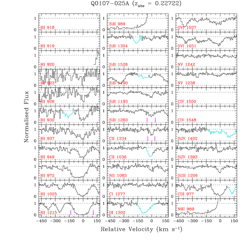
Figure 13: Similar to Fig. 12 but for the $z_{\rm abs}$ $=0.22722$ system towards Q0107–025A. The Lyman series lines below H i$\lambda 937$ fall at the blue edge of the spectrum. These lines require 10–20 km s^-1 velocity shifts in order to be properly aligned with other members of the Lyman series lines. The blue wing of the Ly$\gamma$ line is blended with Galactic Si ii$\lambda 1193$ absorption. The wavelength range corresponding to the Si ii$\lambda 989$ and N iii$\lambda 989$ is affected by geo-coronal Ly$\alpha$ emission. A full-blown multiphase analysis of this absorber is presented in Muzahid (2014). Here we adopt the column densities of relevant ions from Table 1 of Muzahid (2014). Since several unsaturated higher order Lyman series lines are available for this system, the measured $\log N(\mbox{H\,{\sc i}})=15.92\pm 0.08$ has the highest quality factor of $Q=5$.

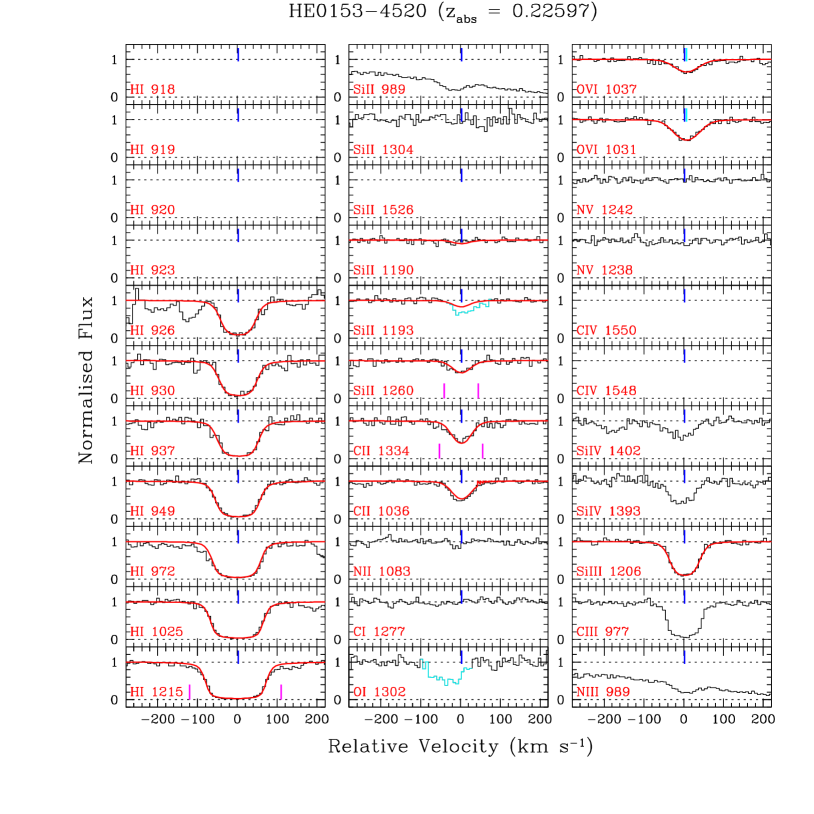
Figure 14: Similar to Fig. 12 but for the $z_{\rm abs}$ $=0.22597$ system towards HE0153–4520. The wavelength range corresponding to the Si ii$\lambda 989$ and N iii$\lambda 989$ is affected by Galactic Ly$\alpha$ absorption. The Si ii$\lambda 1193$ line is blended with an unknown contaminant. The H i$\lambda 937$, $\lambda 930$, and $\lambda 926$ lines fall at the extreme edge of the spectrum. These lines require $\sim$$7$, $\sim$$15$, and $\sim$$30$ km s^-1 velocity shifts, respectively, in order to be aligned with the other Lyman series lines. Voigt profile fitting of the metal lines (i.e., C ii$\lambda 1036$, $\lambda 1334$, Si ii$\lambda 1260$, and Si iii$\lambda 1206$) is performed simultaneously by keeping the $z$ and $b$-parameter of each line tied to the others. Note that the Si iii$\lambda 1206$ line is strongly saturated. We consider the measured $N(\mbox{Si\,{\sc iii}})$ to be a lower limit. A full-blown multiphase analysis of this absorber is presented in Savage et al. (2011). The column densities we obtained for the metal lines are consistent with the values reported in Savage et al. (2011). From the partial Lyman limit break seen in the FUSE spectrum they have constrained $\log N(\mbox{H\,{\sc i}})=16.61^{+0.12}_{-0.17}$. Our single-component, simultaneous fit to the available Lyman series line provides a somewhat higher $N(\mbox{H\,{\sc i}})$ value (i.e., $\log N(\mbox{H\,{\sc i}})=16.83\pm 0.07$) but the two values are consistent within $1.6\sigma$. We thus assign a quality factor of $Q=4$ for the $N(\mbox{H\,{\sc i}})$ that we obtained.

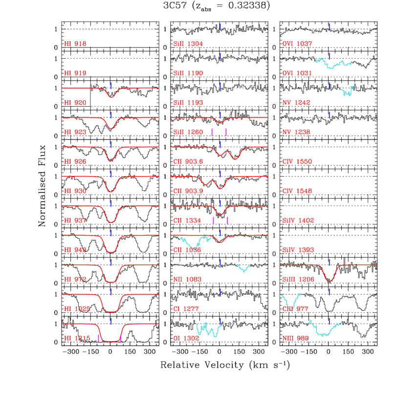
Figure 15: Similar to Fig. 12 but for the $z_{\rm abs}$ $=0.32338$ system towards 3C57. The presence of several unsaturated Lyman series lines permits an accurate $N(\mbox{H\,{\sc i}})$ measurement for the component that shows weak Si ii and C ii absorption. We assign a quality factor of $Q=5$ for this system. The lack of any detectable absorption in the O vi$\lambda 1037$ line near $0$ km s^-1 indicates that the absorption seen in the O vi$\lambda 1031$ must be a blend. Voigt profile fitting for the metal lines is done simultaneously keeping the $z$ and $b$-parameter tied. Note that the Si iii line is strongly saturated and hence the measured $N(\mbox{Si\,{\sc iii}})$ is considered to be a conservative lower limit.

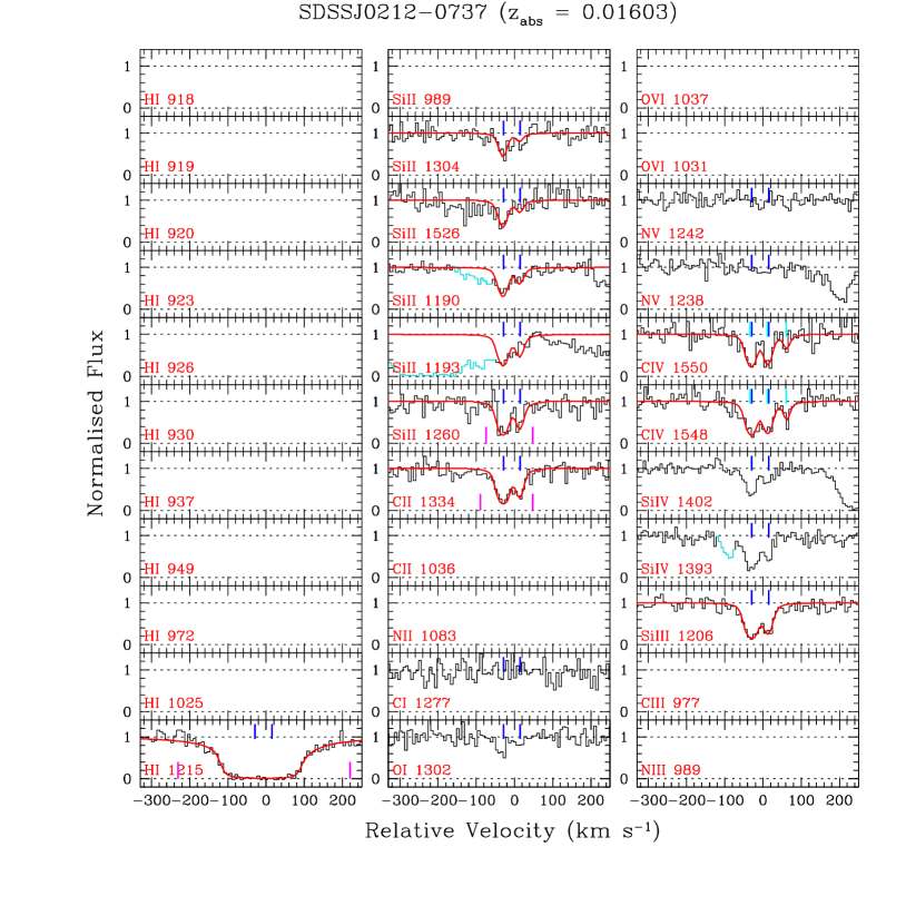
Figure 16: Similar to Fig. 12 but for the $z_{\rm abs}$ $=0.01603$ system towards SDSSJ0212–0737. Besides low-ions, strong C iv and Si iv lines are detected. The Si ii$\lambda 1193$ line is blended with the strong O vi $\lambda 1031$ absorption at $z_{\rm abs}$ $=0.17403$, intrinsic to the background QSO. We note that the Si ii$\lambda 1304$ and O i$\lambda 1302$ lines require a velocity shift of $\sim-7$ km s^-1 with respect to the Si iii. Additionally, the C ii$\lambda 1334$ line is shifted by $\sim-3$ km s^-1. All the metal lines are fitted simultaneously using two Voigt profile components. The component at $\sim-30$ km s^-1 is strongly saturated for both the C ii$\lambda 1334$ and Si iii$\lambda 1206$ lines. In fact, the C ii$\lambda 1334$ line is heavily saturated in both components. However, $N(\mbox{Si\,{\sc ii}})$ is adequately determined due to the presence of weaker Si ii lines (e.g. $\lambda 1304$). The Ly$\alpha$ profile and the presence of the O i$\lambda 1302$ line indicate a high $N(\mbox{H\,{\sc i}})$. We believe that the estimated $N(\mbox{H\,{\sc i}})$, using a two-component fit, is reasonably constrained from the wings of the Ly$\alpha$ absorption. We assign $Q=3$ for this system.

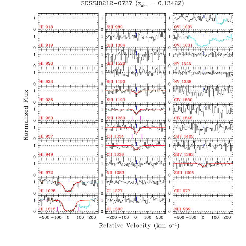
Figure 17: Similar to Fig. 12 but for the $z_{\rm abs}$ $=0.13422$ system towards SDSSJ0212–0737. The absorption seen in the O vi$\lambda 1031$ panel is actually Ly$\beta$ from the $z_{\rm abs}$ $=0.14107$ system. We note that there is a velocity offset of $\sim$$10$ km s^-1 between the Ly$\alpha$ and Ly$\beta$ absorption lines. The metal lines are fitted simultaneously keeping $z$ and $b$-parameter tied. Similarly, we perform a simultaneous fit to the Ly$\alpha$ and Ly$\beta$ lines. Because the Ly$\beta$ absorption is only mildly saturated, with total $\log N(\mbox{H\,{\sc i}})=14.95\pm 0.08$, we assign a quality factor of $Q=3$.

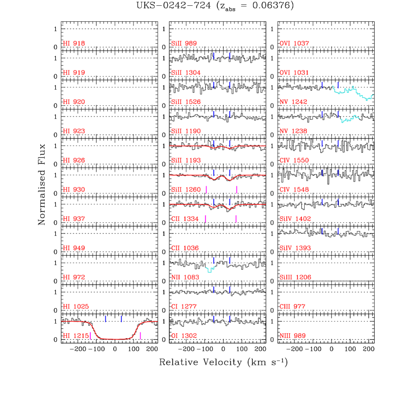
Figure 18: Similar to Fig. 12 but for the $z_{\rm abs}$ $=0.06376$ system towards UKS–0242–724. The Si iii$\lambda 1206$ line falls on a spectral gap. Both the Si ii and C ii lines show a two-component structure. All three metal transitions are fitted simultaneously keeping the $z$ and $b$-parameter tied to each other. Apart for Ly$\alpha$, no other Lyman series lines are covered by the spectrum. We have used two components to fit the Ly$\alpha$ line using component redshifts obtained from the metal line fitting. Since the Ly$\alpha$ profile is heavily saturated and no higher order Lyman series lines are available, the estimated $N(\mbox{H\,{\sc i}})$ is assigned the lowest quality factor of $Q=1$.

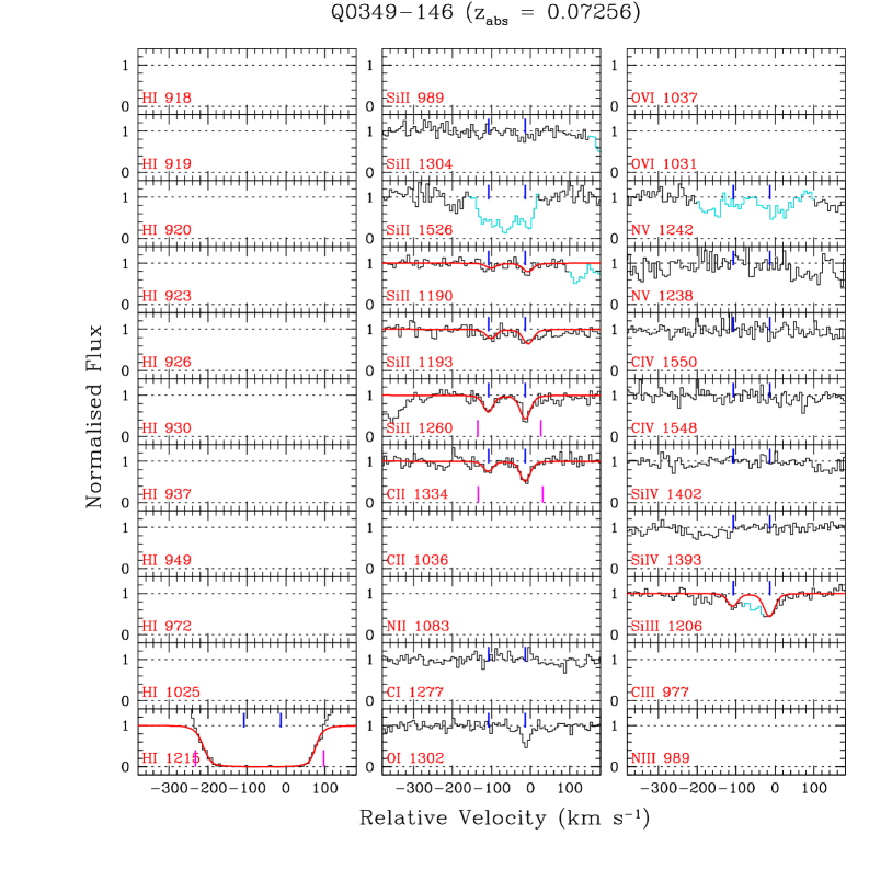
Figure 19: Similar to Fig. 12 but for the $z_{\rm abs}$ $=0.07256$ system towards Q0349–146. The absorption seen in the Si ii$\lambda 1526$ panel is the Si iii$\lambda 1206$ line of the $z_{\rm abs}$ $=0.35687$ system. The Si ii$\lambda 1260$ and C ii$\lambda 1334$ lines are $\sim+8$ km s^-1 and $\sim-13$ km s^-1 offset with respect to the Si iii line, respectively. The Si ii and C ii lines show two-component absorption kinematics. There is some absorption in-between the two components in the Si iii line which is likely to be a blend. All the metal lines are fitted simultaneously. The presence of narrow O i line in the stronger component indicates a high $N(\mbox{H\,{\sc i}})$ value. The Ly$\alpha$ line falls in between the geo-coronal O i$\lambda 1302$ and Si ii$\lambda 1304$ emission lines. We used two Voigt profile components, as seen in the C ii/Si ii lines, with redshifts locked at the values obtained from the metal-line fitting, in order to fit the Ly$\alpha$ profile. This system is assigned a quality factor of $Q=1$, since we could not determine the H i column density adequately.

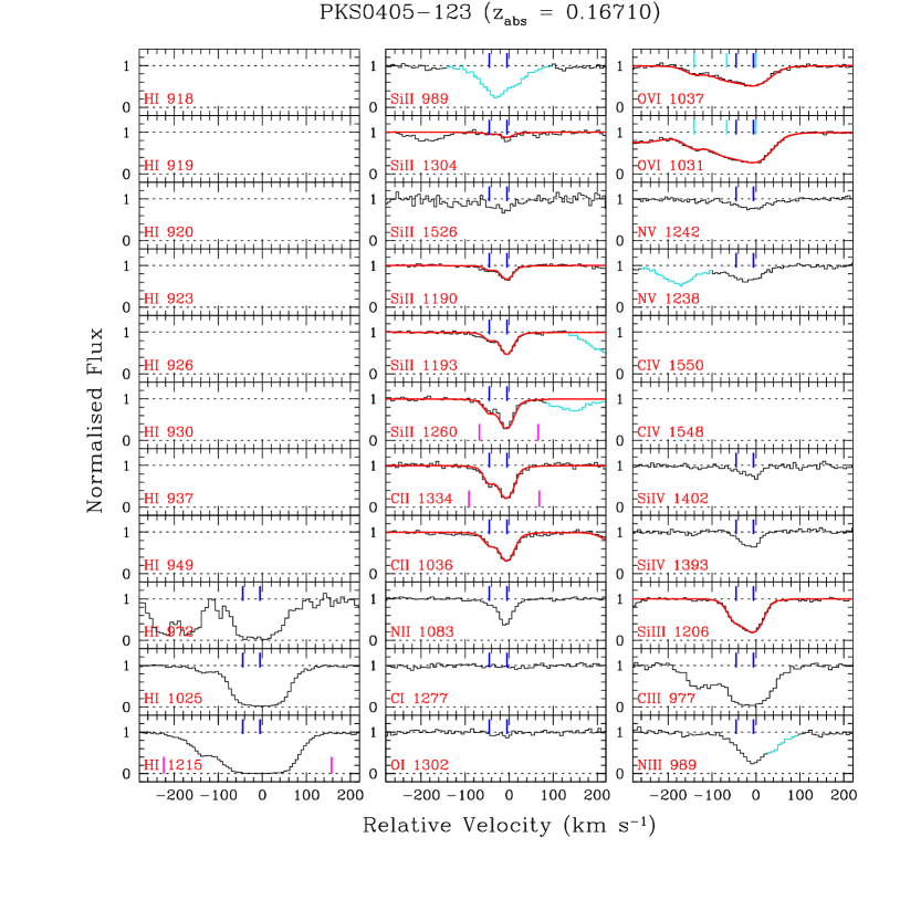
Figure 20: Similar to Fig. 12 but for the $z_{\rm abs}$ $=0.16710$ system towards PKS0405–123. This system has been studied by several authors (e.g., Prochaska et al., 2004; Savage et al., 2010). A full-blown multiphase analysis of this absorber is presented in Savage et al. (2010). This particular spectrum has a serious wavelength-alignment problem. However, the high spectral $\rm S/N$, and relatively simple and uncontaminated absorption kinematics make it easy to understand the nature of the wavelength calibration uncertainty. From the partial Lyman limit break observed in a fuse spectrum, Prochaska et al. (2004) have constrained the total $\log N(\mbox{H\,{\sc i}})=16.45\pm 0.05$. Here we adopt this $N(\mbox{H\,{\sc i}})$ value and do not attempt to estimate $N(\mbox{H\,{\sc i}})$ from the COS spectrum since all three Lyman series lines are heavily saturated. We assign $Q=5$ for this absorber. The different transitions of C ii and Si ii are fitted simultaneously keeping $z$ and $b$-parameters tied. Si iii, however, requires somewhat higher $b$-values. The total column densities we estimate for the metal lines are consistent with the measurements of Savage et al. (2010). Both the C ii and Si iii lines are strongly saturated. We consider both $N(\mbox{C\,{\sc ii}})$ and $N(\mbox{Si\,{\sc iii}})$ as conservative lower limits (see also Savage et al., 2010).

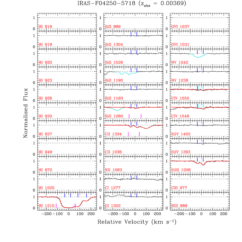
Figure 21: Similar to Fig. 12 but for the $z_{\rm abs}$ $=0.00369$ system towards IRAS–F04250–5718. Very weak C ii$\lambda 1334$, Si ii$\lambda 1260$, Si iii, and C iv doublet lines are detected. The red wing of the C ii$\lambda 1334$ line is blended, possibly with the Ly$\alpha$ of an associated absorber at $z_{\rm abs}$ $=0.10220$. Our fit to the C ii$\lambda 1334$ line is corrected for the contaminating absorption. Except for the Ly$\alpha$, no other Lyman series lines are covered. We use the line centroids and $b$-parameters of the Si iii lines to fit the main Ly$\alpha$ absorption clump. In addition, two weak Ly$\alpha$ components are required to fit the red wing. Since the main Ly$\alpha$ absorption clump which is related to the metal lines is heavily saturated, we assign a quality factor of $Q=1$ for this system.

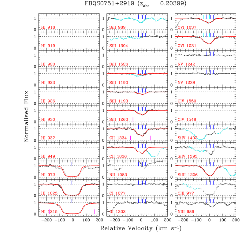
Figure 22: Similar to Fig. 12 but for the $z_{\rm abs}$ $=0.20399$ system towards FBQS 0751+2919. Besides several weak low-ionization lines, strong O vi is detected, however, no N v is present. The N ii$\lambda 1083$ absorption is severely affected by the geo-coronal O i emission. The blue wing of the C iii line is possibly blended with the Ly$\beta$ of the $z_{\rm abs}$ $=0.14644$ system. The strong absorption redward of the C ii$\lambda 1036$ line is the Ly$\alpha$ from the $z_{\rm abs}$ $=0.02673$ system. The blue wings of the Si iv$\lambda 1393$ and $\lambda 1402$ are blended by the higher order Lyman series lines (i.e., H i$\lambda 917$ and $\lambda 923$, respectively) from the $z_{\rm abs}$ $=0.82912$ system. We note that the lines with rest-frame wavelength $\lesssim 1050$ Å require a velocity shift of $\sim-12$ km s^-1. A minimum of three components is required to fit the C ii and Si ii lines simultaneously. The Si iii line is strongly saturated and required larger component $b$-values compared to the singly ionized metal ions, suggesting an additional contribution from other gas phase(s). The measured $N(\mbox{Si\,{\sc iii}})$ should be treated as a lower limit. The available Lyman series lines are heavily saturated. We have performed both single-component and three-component fits to the Lyman series lines. A single-component fit gives $\log N(\mbox{H\,{\sc i}})=17.77\pm 0.05$ and $b(\mbox{H\,{\sc i}})=24$ km s^-1. A three-component fit, on the other hand, gives an order of magnitude lower $N(\mbox{H\,{\sc i}})$ of $10^{16.67\pm 0.08}$ cm^-2. We adopted the single component fit results keeping in mind that the true $N(\mbox{H\,{\sc i}})$ could only be less. We assign a quality factor of $Q=2$ for the system.

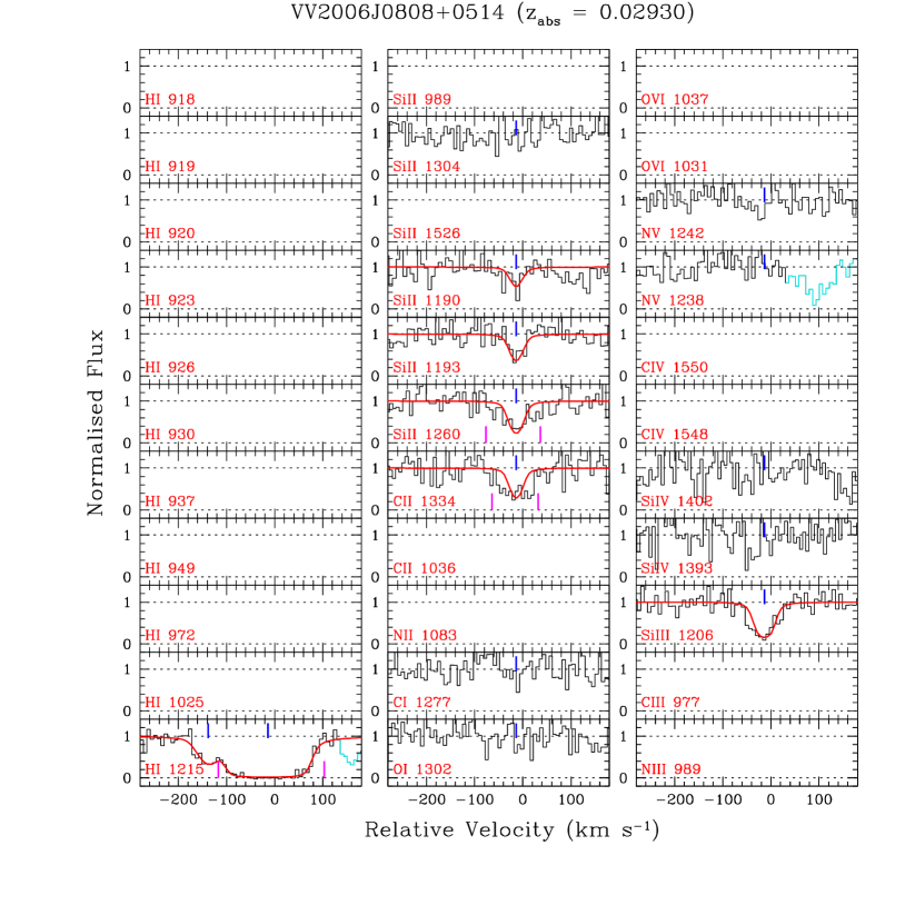
Figure 23: Similar to Fig. 12 but for the $z_{\rm abs}$ $=0.02930$ system towards VV2006 J0808+0514. The C iv doublet is not covered since the spectrum is taken only with the G130M grating covering up to $1460$ Å (observed). The spectrum looks noisy, however, consistent metal absorption lines are detected. First we fit the Si ii lines ($\rm\lambda 1190,\lambda 1193,and\lambda 1260$) simultaneously. We then use the best-fitting $z$ and $b$-parameter to fit the C ii$\lambda 1334$ and Si iii$\lambda 1206$ lines. The C ii line might have contributions from other unknown and unrelated absorption. We consider the measured $N(\mbox{C\,{\sc ii}})$ as a conservative upper limit. The Si iii line is heavily saturated and hence $N(\mbox{Si\,{\sc iii}})$ should be treated as a lower limit. The $N(\mbox{H\,{\sc i}})$ we estimate from the Ly$\alpha$ profile alone ($\log N(\mbox{H\,{\sc i}})=17.57\pm 0.43$) is highly uncertain. We assign a quality factor of $Q=1$ for this system.

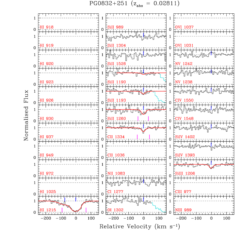
Figure 24: Similar to Fig. 12 but for the $z_{\rm abs}$ $=0.02811$ system towards PG 0832+251. This is a very weak metal line absorber. Except for the C ii$\lambda 1334$, which requires a velocity shift of $\sim+5$ km s^-1, all other lines are well aligned. The Ly$\alpha$ line, which is only mildly saturated, exhibits an extra broad, weak component in the blue wing. Since the Ly$\alpha$ is not heavily saturated we assign a quality factor of $Q=2$ for this system.

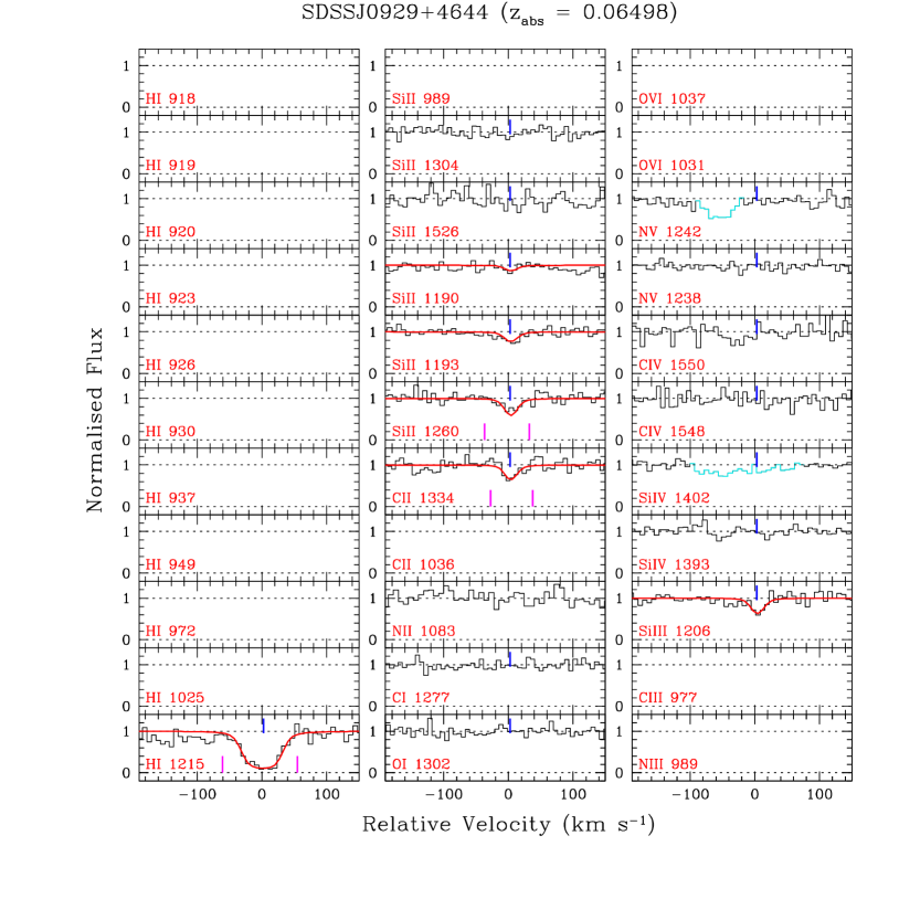
Figure 25: Similar to Fig. 12 but for the $z_{\rm abs}$ $=0.06498$ system towards SDSS J0929+4644. Single-component, weak metal lines are fitted simultaneously keeping $z$ and $b$-parameter tied. The Ly$\alpha$ is narrow, only mildly saturated, and off center by 8 km s^-1 with respect to C ii/Si ii. We assign a quality factor of $Q=2$ for this system.

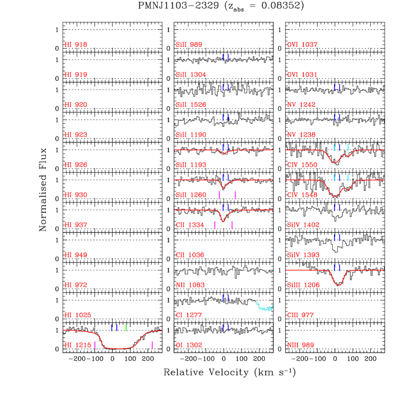
Figure 26: Similar to Fig. 12 but for the $z_{\rm abs}$ $=0.08352$ system towards PMNJ1103–2329. Besides the low-ionization lines, multi-component, strong C iv and Si iv lines are present. The spectrum at $\sim-200$ km s^-1 in the Si iii$\lambda 1206$ panel is affected by the geo-coronal O i+Si ii emission lines. A minimum of two components is required to fit the metal lines simultaneously. The strength of the Si iii absorption indicates that the line is heavily saturated. Therefore, the $N(\mbox{Si\,{\sc iii}})$ should treated as a lower limit. In addition to the two components seen in the low-ionization lines, the heavily saturated Ly$\alpha$ line requires a broad component at $\sim+80$ km s^-1, corresponding to the C iv$/$Si iv component seen at the same velocity. Some amount of Si iii may be present in this component as indicated by the spiky absorption we ignored in our analysis. However, the contribution of such a weak component to the total $N(\mbox{Si\,{\sc iii}})$ would be negligible. A free $b$-parameter fit to the Ly$\alpha$ profile was unstable. Thus, for estimating $N(\mbox{H\,{\sc i}})$ associated with the two components that are aligned with the low-ions, we assumed $b(\mbox{H\,{\sc i}})=18.2$, corresponding to $T=2\times 10^{4}$ K, for each component and determined the maximum $N(\mbox{H\,{\sc i}})$ that can be accommodated within the observed profile, one-by-one. This allow us to put an upper limit on the $N(\mbox{H\,{\sc i}})$. Due to the absence of the higher order Lyman series lines, we assign the lowest quality factor (i.e. $Q=1$) for this system.

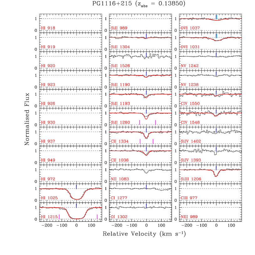
Figure 27: Similar to Fig. 12 but for the $z_{\rm abs}$ $=0.13850$ system towards PG1116+215. This is a narrow, weak, single component system. We note that the lines with rest-frame wavelength $<1040$ Å require a $\sim-9$ km s^-1 velocity shift. The metal lines are fitted simultaneously keeping the $z$ and $b$-parameter tied. We notice that the Si ii$\lambda 1260$ line falls on top of the QSO’s Ly$\alpha$+N v emission line. The apparent mismatch between the data and the model profile for the Si ii$\lambda 1260$ line could be due to the fact that the absorber is not fully covering the broad emission line region of the background QSO (i.e., the partial coverage effect, see e.g., Muzahid et al. (2012)). This would indicate that the size of the absorber is very small. However, the possibility of unresolved saturation of the Si ii$\lambda 1260$ line and/or uncertainty in the continuum placement also cannot be ruled out. The constraint on $N(\mbox{Si\,{\sc ii}})$ comes from the other weaker transitions, in particular, from the Si ii$\lambda 1190$ line. FUSE and STIS observations of the full Lyman series lines (i.e., Ly$\alpha$–H i$\lambda 916$) are presented by Sembach et al. (2004). Here we adopted their best-fitting COG value of $\log N(\mbox{H\,{\sc i}})=16.20\pm 0.05$ and assign the highest quality factor of $Q=5$.

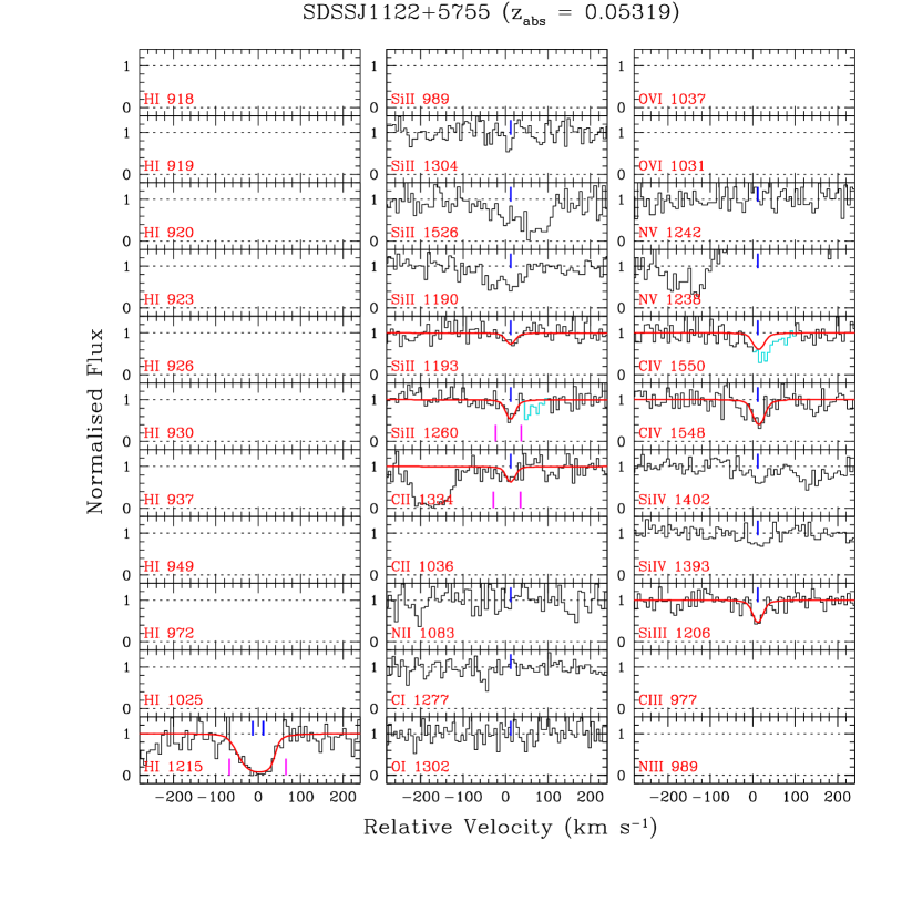
Figure 28: Similar to Fig. 12 but for the $z_{\rm abs}$ $=0.05319$ system towards SDSSJ1122+5755. The absorption seen in the Si ii$\lambda 1190$ and $\lambda 1526$ panels actually arise from the Galactic S ii$\lambda 1253$ and Fe ii$\lambda 1608$ lines, respectively. The wavelength rage of N v$\lambda 1238$ is affected by the geo-coronal O i+Si ii emission lines. The single component, weak metal lines are fitted simultaneously keeping $z$ and $b$-parameters tied. Besides the weak low-ionization lines, strong C iv and weaker Si iv lines are detected. The Ly$\alpha$ absorption shows an asymmetric profile indicating the presence of more than one component. We used two components to fit the Ly$\alpha$ profile. vpfit returns a large error ($\sim 1.5$ dex) in $N(\mbox{H\,{\sc i}})$. We assigned $Q=1$ for this system.

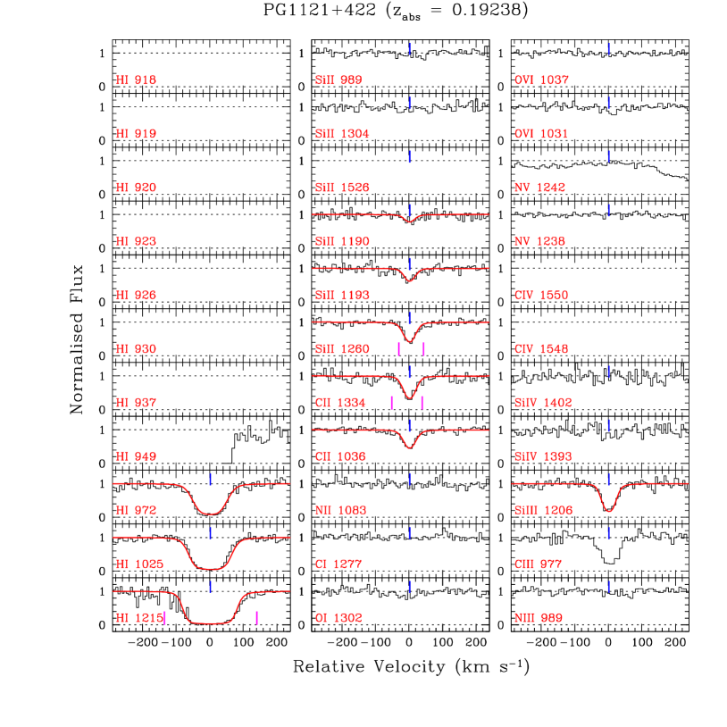
Figure 29: Similar to Fig. 12 but for the $z_{\rm abs}$ $=0.19238$ system towards PG1121+422. Single-component metal lines are fitted simultaneously keeping $z$ and $b$-parameters tied with each other. The Si iii line is mildly saturated. We note that the C ii$\lambda 1036$ and Ly$\beta$ lines require a velocity shift of $\sim-11$ km s^-1 in order to be aligned with the other metal lines. All three Lyman series lines are heavily saturated. We obtained a solution with $\log N(\mbox{H\,{\sc i}})=15.64\pm 0.05$ and $b(\mbox{H\,{\sc i}})=37\pm 1$ km s^-1 using a simultaneous, single-component fit. Since all three Lyman series lines are saturated we assign $Q=2$ for this system.

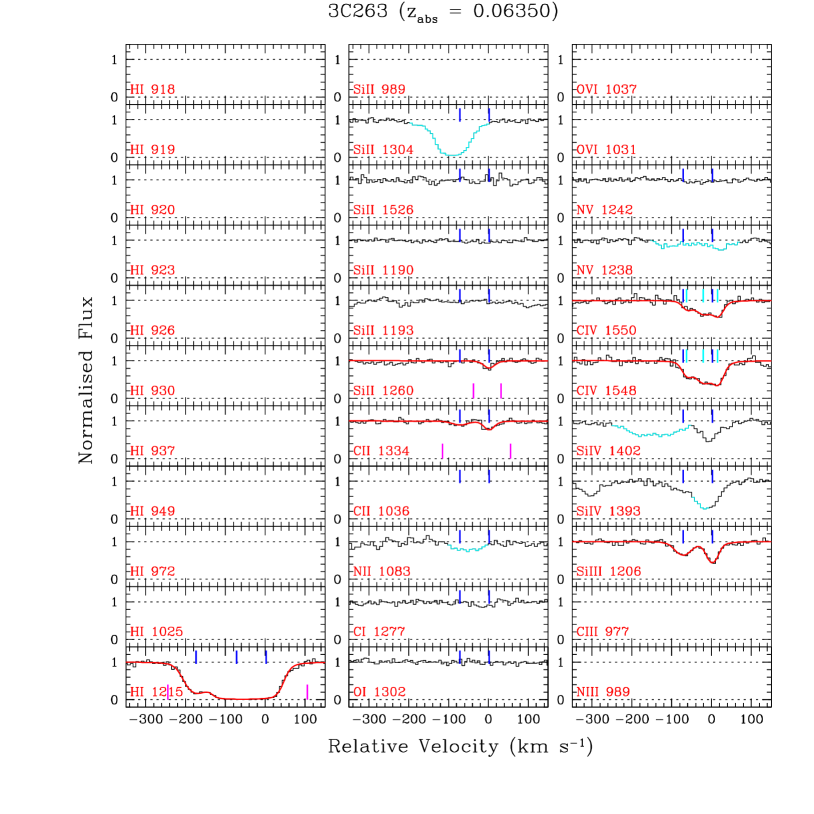
Figure 30: Similar to Fig. 12 but for the $z_{\rm abs}$ $=0.06350$ system towards 3C263. Both the Si iii and C ii$\lambda 1334$ lines clearly show a two-component structure. The component at $\sim-70$ km s^-1, however, is not detected in the Si ii$\lambda 1260$ line. Strong C iv$\lambda\lambda 1548,1550$ lines are present along with Si iv$\lambda\lambda 1393,1402$. The Si iv$\lambda 1393$ line is possibly blended with the Ly$\alpha$ of the $z_{\rm abs}$ $=0.21926$ system. The blue wing of the Si iv$\lambda 1402$ line is blended with the Ly$\beta$ of the $z_{\rm abs}$ $=0.45374$ system. Metal lines are fitted simultaneously. The Ly$\alpha$ line is fitted using three components, with two of them locked at the redshifts of the metal line components. An extra H i component is required to fit the weak absorption seen at $\sim-180$ km s^-1. However, we adopted the total $\log N(\mbox{H\,{\sc i}})=15.40\pm 0.12$ as measured by the Savage et al. (2012) from the unsaturated Ly$\gamma$ profile using FUSE data. We thus assign a quality factor of $Q=4$ for this system.

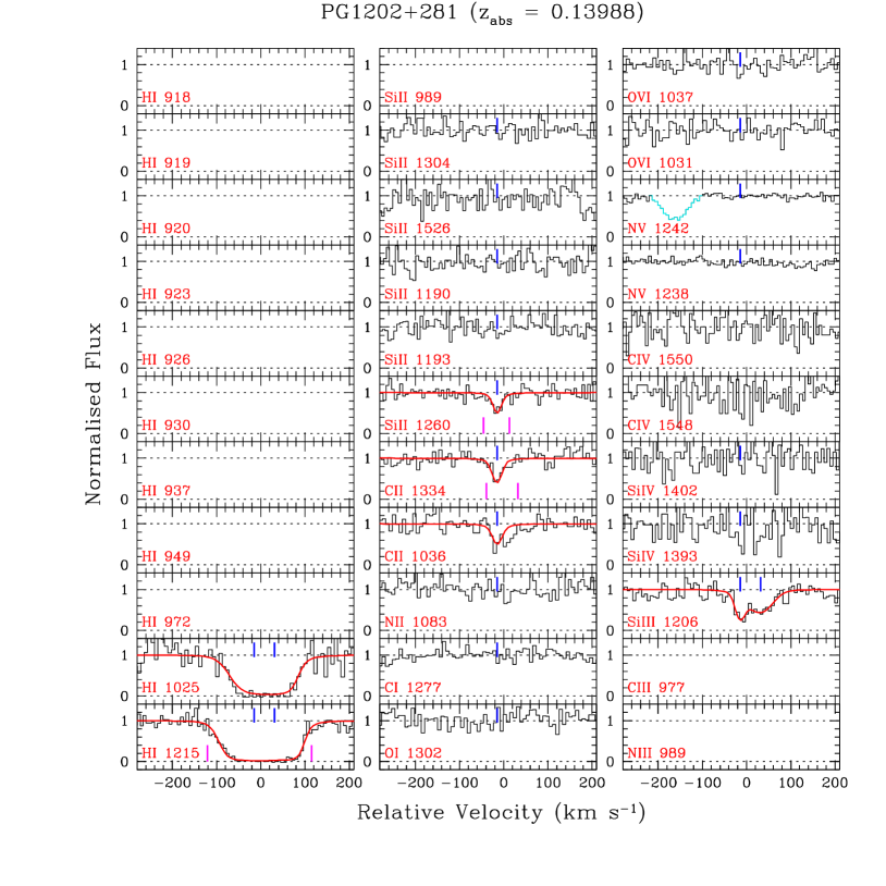
Figure 31: Similar to Fig. 12 but for the $z_{\rm abs}$ $=0.13988$ system towards PG 1202+281. None of the high ionization lines are detected. The Si iii line shows a two component absorption kinematics. The component at $+40$ km s^-1 is not detected in the Si ii$\lambda 1260$, C ii$\lambda 1334$, and C ii$1036$ lines. We note that the C ii$\lambda 1334$ line is offset by $\sim+10$ km s^-1 with respect to the Ly$\alpha$/Si iii line whereas the Ly$\beta$ and C ii$\lambda 1036$ lines are offset by $\sim+20$ km s^-1. The metal lines are fitted simultaneously keeping $z$ and $b$ tied for the component present in all of the transitions. A simultaneous fit is also performed for the Ly$\alpha$ and Ly$\beta$ lines using two Voigt profile components. The redshifts of the components are locked at the values obtained from the Si iii fit. Since both the lines are heavily saturated we assign a quality factor of $Q=1$.

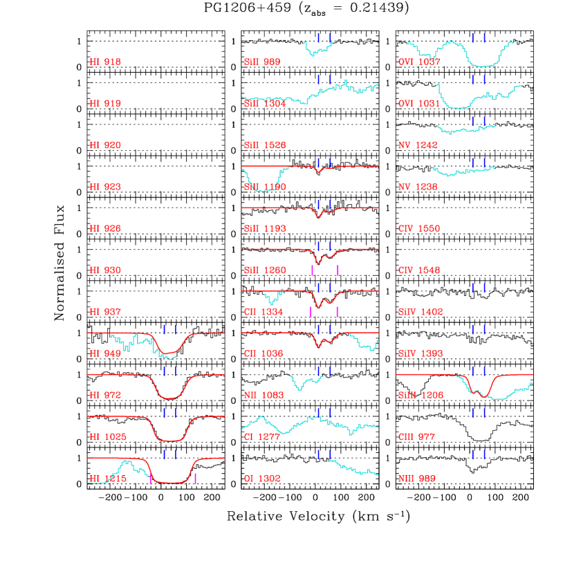
Figure 32: Similar to Fig. 12 but for the $z_{\rm abs}$ $=0.21439$ system towards PG 1206+459. The narrow absorption seen in the blue wing of the Ly$\alpha$ line is the S ii$\lambda 765$ from the $z_{\rm abs}$ $=0.9276$ system. The absorption seen in the N v$\lambda 1238$ panel is actually the Ne viii $\lambda 780$ line from the same system (see Tripp et al., 2011, for details). The Si iii$\lambda 1206$ line is severely blended with the Ly$\alpha$ from the $z_{\rm abs}$ $=0.20575$ system. The absorption in the Si ii$\lambda 1304$ panel is actually the Ne viii $\lambda 780$ line from a known intrinsic absorber at $z_{\rm abs}$ $1.028$ studied by Muzahid et al. (2013). The O vi $\lambda 1031$ line is blended with the Galactic S ii$\lambda 1253$ line and the Ly$\beta$ of the $z_{\rm abs}$ $=0.22156$ system. The absorption in the O vi $\lambda 1037$ panel is the Galactic Si ii $\lambda 1260$ line. So we could not confirm the presence/absence of O vi absorption in this system. This spectrum suffers from a complex velocity alignment problem. However the clean two component structure makes it possible to gauge the uncertainty. The two components seen in the weak metal lines are fitted simultaneously. Since the Si iii line is heavily blended, we have estimated the maximum column density allowed by the profile by keeping the $z$ and $b$-parameters locked at the values we obtained from the fitting of Si ii and C ii lines. The Lyman series lines are also fitted simultaneously using two components with the redshifts locked at the values we obtained for the metal lines. The H i $\lambda 949$ line is partially blended by an unknown contaminant. However, we believe we have an adequate $N(\mbox{H\,{\sc i}})$ measurement for this system with $Q=3$.

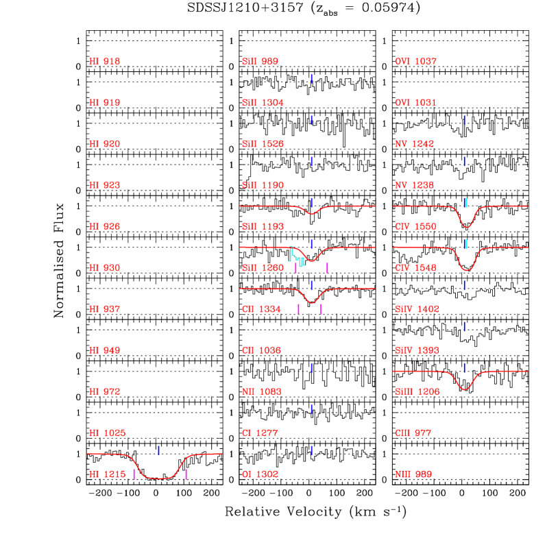
Figure 33: Similar to Fig. 12 but for the $z_{\rm abs}$ $=0.05974$ system towards SDSSJ1210+3157. In addition to the low-ionization lines, strong C iv, and weaker Si iv, and N v lines are detected. The blue wing of the Si ii$\lambda 1260$ is blended with the Galactic C ii*$\lambda 1335$ absorption. The equivalent width of the Si ii line is, thus, calculated from the model profile. The spectrum is very noisy at the position of the Si ii$\lambda 1193$ line. A single component, simultaneous fit is performed for all the metal line transitions. The Ly$\alpha$ line is fitted with a single component with redshift locked with the metal line component. Due to the lack of higher order unsaturated Lyman series lines, we assign $Q=1$ for this system.

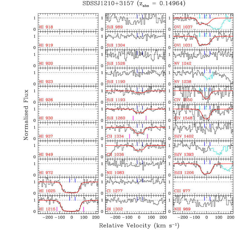
Figure 34: Similar to Fig. 12 but for the $z_{\rm abs}$ $=0.14964$ system towards SDSSJ1210+3157. Besides several low-ionization lines, strong O vi and C iv lines are detected. The O vi$\lambda 1037$ line is blended with the Galactic Si ii$\lambda 1193$ absorption. The absorption seen in the N v$\lambda 1238$ panel is the Ly$\beta$ from the $z_{\rm abs}$ $=0.38854$ associated system. Though the spectrum is noisy, a two component absorption kinematics is clearly seen in the Si iii line. Note that the Si iii line is strongly saturated. Thus the $N(\mbox{Si\,{\sc iii}})$ we obtained from vpfit should be considered as lower limit. Both the Lyman series lines are heavily saturated. We performed simultaneous fitting keeping both $z$ and $b$-parameters locked at the values we obtained from metal line fit. Since both the lines are heavily saturated we assign $Q=1$ for this system.

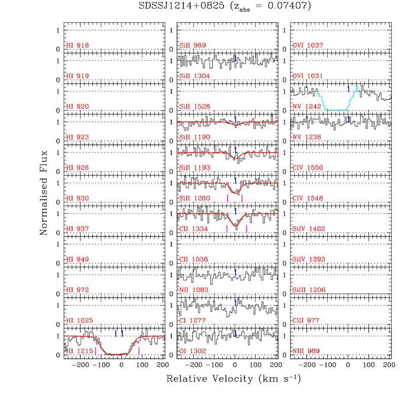
Figure 35: Similar to Fig. 12 but for the $z_{\rm abs}$ $=0.07407$ system towards SDSSJ1214+0825. Only G130M data are available. Si iii falls in the spectral gap. Ly$\alpha$ falls on top of galactic O i+Si ii emission lines. We combined the “night-only" data separately for the Ly$\alpha$ absorption. The C ii and Si ii lines can be fitted simultaneously using only one component. The Ly$\alpha$ absorption require one more component at $\sim-28$ km s^-1. Note that for the component at $0$ km s^-1 we determine the maximum column density allowed by the profile to be $\log N(\mbox{H\,{\sc i}})=15.0$, using a Doppler-parameter that we obtained for the metal lines ($b=22$ km s^-1). We assign a quality factor of $Q=1$ for the $N(\mbox{H\,{\sc i}})$ upper limit. Because of the lack of Si iii coverage, we do not consider this system for PI modeling.

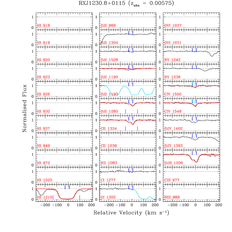
Figure 36: Similar to Fig. 12 but for the $z_{\rm abs}$ $=0.00575$ system towards RXJ 1230.8+0115. Besides low-ions, high-ionization metal lines (C iv and Si iv) are also detected. The Si ii$\lambda 1260$ and C ii$\lambda 1334$ lines are $\sim+6$ and $+4$ km s^-1 offset, respectively, with respect to the Si iii line. The Si ii$\lambda 1193$ line is lost due to the strong Galactic N i$\lambda 1200$ line. The strong line seen in the O i panel is actually Ly$\alpha$ absorption from the $z_{\rm abs}$ $=0.07770$ system. A clear two-component kinematics is seen in the low-ionization metal lines. The metal lines are fitted simultaneously. The Ly$\alpha$ line is fitted using two components with redshifts locked at the values obtained from the metal line fitting. Due to the lack of unsaturated, higher order Lyman series lines, the estimated $N(\mbox{H\,{\sc i}})$ is uncertain, and we assign a quality factor of $Q=1$.

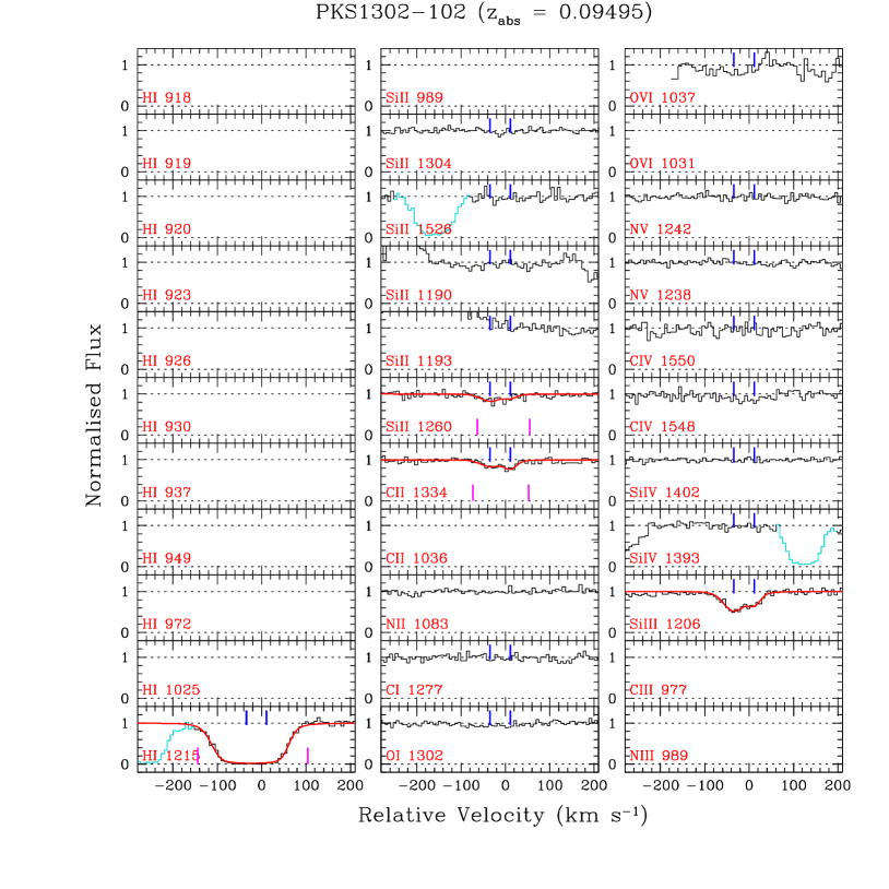
Figure 37: Similar to Fig. 12 but for the $z_{\rm abs}$ $=0.09495$ system towards PKS 1302–102. The presence of high-ionization lines (e.g. C iv/O vi) is not obvious. A minimum of two components is required to fit the low-ionization lines. The C ii$\lambda 1334$ line shows a velocity offset of $\sim-7$ km s^-1 with respect to the other lines. The metal lines (C ii/Si ii) are fitted simultaneously. We use two Voigt profile components to fit the Ly$\alpha$ absorption with line centroids locked at the values we obtained from the metal line fit. This is a partial-Lyman-limit system with $\log N(\mbox{H\,{\sc i}})=16.88\pm 0.03$ as measured by Cooksey et al. (2008) from the COG analysis of the full Lyman series lines using FUSE data. We adopted their $N(\mbox{H\,{\sc i}})$ value and assign the highest quality factor of $Q=4$.

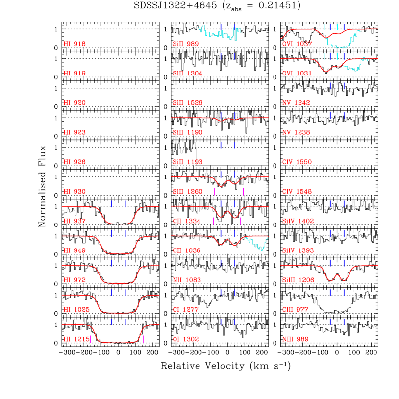
Figure 38: Similar to Fig. 12 but for the $z_{\rm abs}$ $=0.21451$ system towards SDSSJ1322+4645. The Si ii$\lambda 1193$ line falls in the spectral gap. The O vi$\lambda 1031$ line is blended with the Galactic S ii$\lambda 1253$ line, whereas, the O vi$\lambda 1037$ line is lost in the strong Galactic Si ii$\lambda 1260$ absorption. The spectrum is noisy. We used two components to fit the metal lines simultaneously. Both the C ii$\lambda 1334$ and $\lambda 1036$ lines are shifted by $\sim-10$ km s^-1 with respect to the Si iii/Si ii lines. We consider $N(\mbox{Si\,{\sc iii}})$ as upper limit since the Si iii line is strongly saturated. The H i$\lambda 937$ line falls at the extreme blue end of the spectrum. The line require a velocity shift of $\sim+12$ km s^-1. The Lyman series lines are also fitted simultaneously using two components by keeping redshifts locked but allowing $b$-parameters to vary. We, however, adopt the $N(\mbox{H\,{\sc i}})$ value obtained from the Lyman limit break by Prochaska et al. (2017). We assign $Q=4$ for this system.

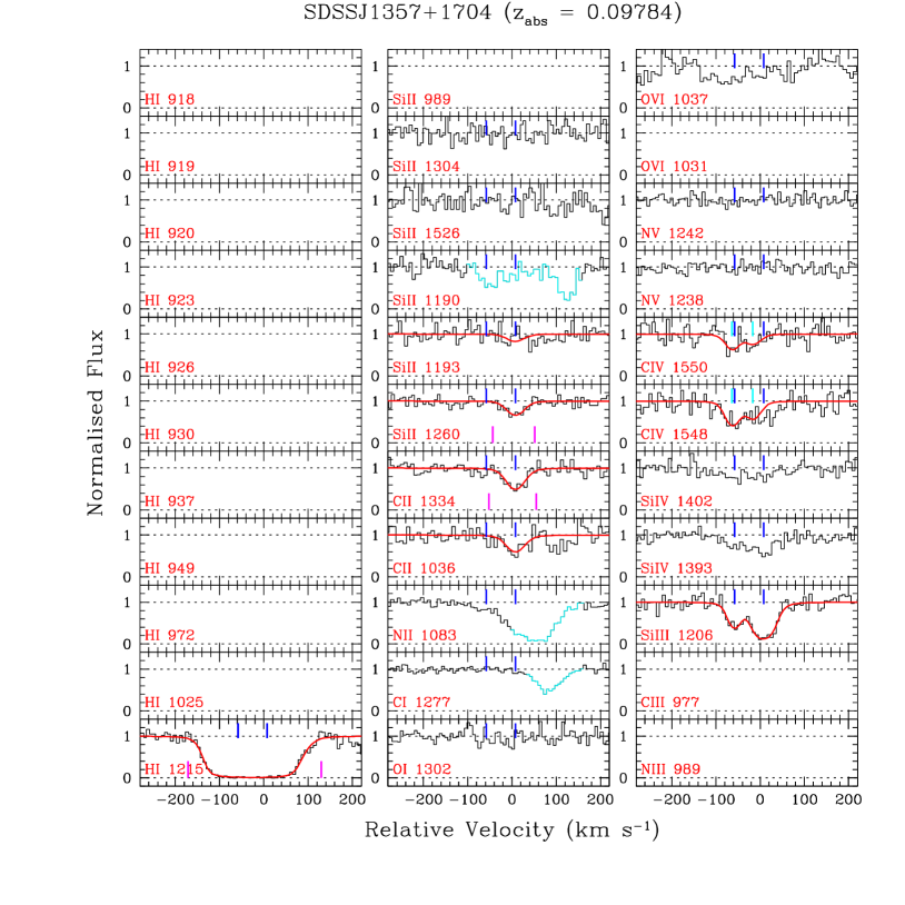
Figure 39: Similar to Fig. 12 but for the $z_{\rm abs}$ $=0.09784$ system towards SDSSJ1357+1704. A two-component absorption kinematics, as seen in the Si iii line, is also present in the Si iv and C iv doublets. However the N v doublet is not detected. The O vi$\lambda 1031$ is not covered. Both C ii$\lambda 1036$ and O vi$\lambda 1037$ fall at the extreme blue end of the spectrum. We note that the C ii$\lambda 1036$ (and hence the O vi$\lambda 1037$) line require a velocity shift of $\sim+15$ km s^-1. Although some absorption is seen in the O vi$\lambda 1037$ panel, we could not confirm its association with this system. The N ii$\lambda 1083$ line is blended with the Galactic Si ii$\lambda 1190$ line. Note that the Si iii component at $\sim 0$ km s^-1 is strongly saturated. The other component is not detected in the singly ionized carbon and silicon lines. The component at $\sim 0$ km s^-1 is fitted simultaneously keeping $z$ and $b$-parameter tied. Due to saturation, we consider $N(\mbox{Si\,{\sc iii}})$ as a lower limit. The Ly$\alpha$ line is fitted with two components as seen in the Si iii line. We note that the Ly$\alpha$ line is contaminated with Galactic C ii$\lambda 1334$. Therefore, the $N(\mbox{H\,{\sc i}})$ in this system is highly uncertain. We thus assign $Q=1$ for this system.

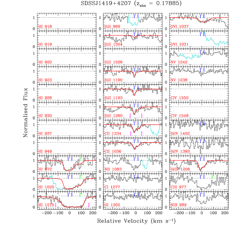
Figure 40: Similar to Fig. 12 but for the $z_{\rm abs}$ $=0.17885$ system towards SDSSJ1419+4207. The Si iii and Ly$\alpha$ lines fall at the red edge of the G130M grating data. Both these lines require a velocity shift of $\sim-11$ km s^-1. The Si iii, C ii$\lambda 1036$ and $\lambda 1334$ lines show one narrow and one broad component. The presence of the broad component is not obvious in the Si ii lines, particularly in the weaker lines. Metal lines are fitted simultaneously using two Voigt profile components. Note that we did not use the Si ii$\lambda 1304$ and $\lambda 989$ lines for fitting, because of blends. The Si ii$\lambda 989$ is blended with the N iii$\lambda 989$ line. The blue wing of the Ly$\beta$ line is blended with the H i$\lambda 937$ line of another intervening system at $z_{\rm abs}$ $=0.28901$. The narrow component is saturated in the C ii and Si iii lines. Thus, both $N(\mbox{C\,{\sc ii}})$ and $N(\mbox{Si\,{\sc iii}})$ are considered as lower limits. Besides the two components seen in the metal lines, the Lyman series lines require an extra component at $\sim+80$ km s^-1, as indicated by the green tick. This additional component may be present in the C iii line. Recently, Prochaska et al. (2017) have published new $N(\mbox{H\,{\sc i}})$ measurement for this system using the Lyman limit break seen in the G140L spectrum. We adopt their $N(\mbox{H\,{\sc i}})$ value of $10^{16.63^{+0.09}_{-0.30}}$ cm^-2 and assign $Q=4$.

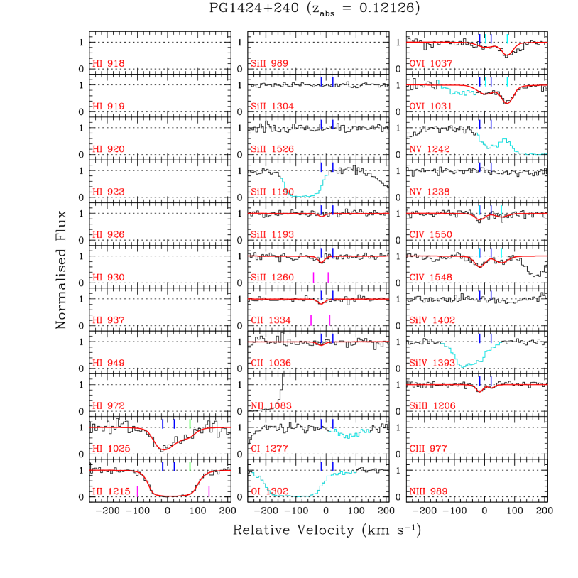
Figure 41: Similar to Fig. 12 but for the $z_{\rm abs}$ $=0.12126$ system towards PG 1424+240. Two very weak components are detected in the Si iii absorption. The weaker component at $\sim+20$ km s^-1, however, is not present in the C ii/Si ii absorption. We note that the C ii$\lambda 1334$ line requires a $\sim-10$ km s^-1 velocity shift. Metal lines are fitted simultaneously keeping $z$ and $b$-parameters tied for the component seen in all three transitions. Besides the weak low-ionization metal lines, C iv and O vi are also detected in this system, but Si iv is not detected. The absorption seen in the Si iv$\lambda 1393$ panel is the Ly$\alpha$ of the $z_{\rm abs}$ $=0.28523$ system. The N ii$\lambda 1083$ line is lost due to geo-coronal Ly$\alpha$ emission. In addition to the two low-ionization metal line components, one more component, shown by the green tick, is required to fit the Ly$\alpha$ and Ly$\beta$ lines simultaneously. This additional component is also evident in the O vi absorption. Since the Ly$\beta$ line is only mildly saturated we assign $Q=3$ for this system.

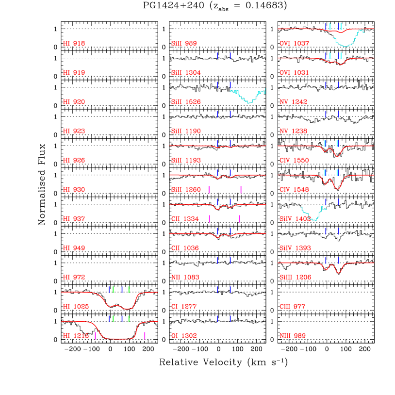
Figure 42: Similar to Fig. 12 but for the $z_{\rm abs}$ $=0.14683$ system towards PG 1424+240. This is a very weak metal line system with high-ionization lines (Si iv, C iv, and O vi) detected. The O vi$\lambda 1031$ line is blended with the Galactic Si ii$\lambda 1190$ line. Two-component absorption kinematics is evident from the Si iii  line. Metal lines are fitted simultaneously by keeping $z$ and $b$-parameters tied. Interestingly, the centroids of the metal line components are not centered around the Ly$\alpha$ and Ly$\beta$ lines. In fact, they are shifted towards the blue wings. This is not due to the wavelength calibration uncertainty since the C ii$\lambda 1036$ (close to the Ly$\beta$ wavelength) and the Si iii (close to the Ly$\alpha$ wavelength) lines are properly aligned. Consequently, the Ly$\alpha$/Ly$\beta$ lines require two additional components, as marked by the green ticks, for an adequate fit. Since there are not enough Lyman series lines to constrain our four-component fit, we assign $Q=1$ for this system.

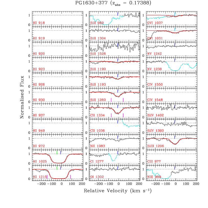
Figure 43: Similar to Fig. 12 but for the $z_{\rm abs}$ $=0.17388$ system towards PG 1630+377. In addition to low-ionization metal lines, O vi is detected. The O vi$\lambda 1031$ (and C ii$\lambda 1036$) line is affected by Galactic Ly$\alpha$ absorption. The strong absorption seen in the N v$\lambda 1238$ panel is the Ly$\beta$ of the $z_{\rm abs}$ $=0.41778$ system. We note that the Ly$\beta$ and O vi lines require a $\sim-20$ km s^-1 velocity shift for properly alignment with the Ly$\alpha$ line. The metal lines are fitted simultaneously. The Doppler parameter of $35$ km s^-1 for our adopted single-component fit probably indicates the presence of multiple unresolved components. Two components are required to fit the Ly$\alpha$ and Ly$\beta$ absorption simultaneously. One of them is locked at the redshift corresponding to the low-ionization metal line component. The other component is possibly arising from the O vi bearing gas phase as indicated by the green vertical tick. Since both the Lyman series lines are heavily saturated we assign $Q=1$ for this system.

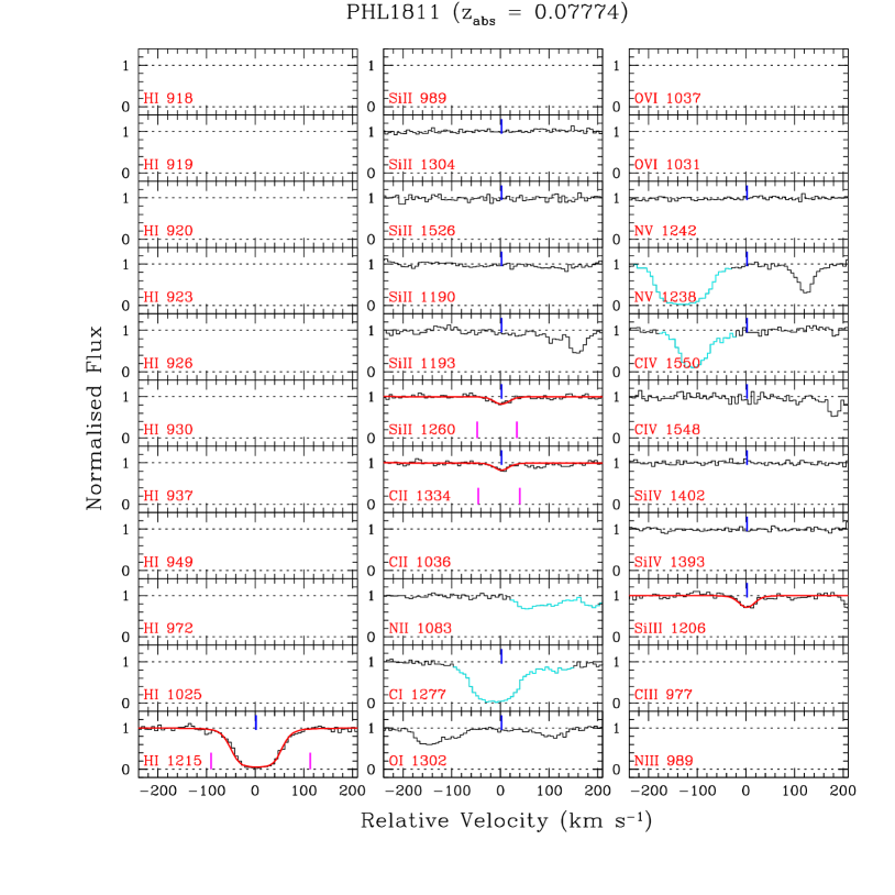
Figure 44: Similar to Fig. 12 but for the $z_{\rm abs}$ $=0.07774$ system towards PHL1811. The low ionization metal lines are very weak. No high ionization metal lines are detected. Using unsaturated higher-order Lyman series lines (up to H i$\lambda 923$) covered by FUSE data and Ly$\alpha$ from STIS data, Lacki & Charlton (2010) have derived $\log N(\mbox{H\,{\sc i}})=16.00\pm 0.05$. Here we adopt their value and assign $Q=5$ for this system.

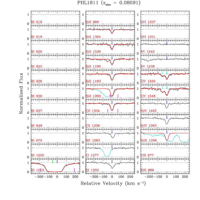
Figure 45: Similar to Fig. 12 but for the $z_{\rm abs}$ $=0.08091$ system towards PHL1811. The Si iii line is blended with Galactic Si ii$\lambda 1304$. The Si ii$\lambda 1260$ line is blended with the Ly$\alpha$ of the $z_{\rm abs}$ $=0.12051$ system. The single component C ii and Si ii lines are fitted simultaneously. We did not use the Si ii$\lambda 1260$ line for fitting because of the blend; but the model profile corresponding to the best fitting parameters is shown. The C ii$\lambda 1034$ line is heavily saturated. The Si ii$\lambda 1193$ also shows an unresolved saturation effect. However the weaker, unsaturated Si ii$\lambda 1304$ line gives an accurate $N(\mbox{Si\,{\sc ii}})$ estimate. Due to a severe blend in the Si iii line we use the best fitting metal line parameters and estimate the maximum $N(\mbox{Si\,{\sc iii}})$ allowed by the observed profile. In addition to the component seen in the low ionization metal lines, Ly$\alpha$ requires another component at $\sim-50$ km s^-1. This component is seen in the high-ionization C iv lines and is indicated by the green ticks. A strong Lyman limit break corresponding to this system is seen in a FUSE spectrum (see Fig. 1 of Jenkins et al., 2003). Ignoring the blue component Jenkins et al. (2005) have derived $\log N(\mbox{H\,{\sc i}})=17.98\pm 0.05$ for the red component at $0$ km s^-1. It is consistent with our measurement (i.e. $\log N(\mbox{H\,{\sc i}})=17.94\pm 0.07$) for that component. We therefore assign $Q=4$ for this system.

References

- Adelberger et al. (2005) Adelberger K. L., Shapley A. E., Steidel C. C., Pettini M., Erb D. K., Reddy N. A., 2005, ApJ, 629, 636
- Asplund et al. (2009) Asplund M., Grevesse N., Sauval A. J., Scott P., 2009, ARA&A, 47, 481
- Becker et al. (2012) Becker G. D., Sargent W. L. W., Rauch M., Carswell R. F., 2012, ApJ, 744, 91
- Bergeron (1986) Bergeron J., 1986, A&A, 155, L8
- Bergeron & Boissé (1991) Bergeron J., Boissé P., 1991, A&A, 243, 344
- Blanton et al. (2003a) Blanton M. R., Lin H., Lupton R. H., Maley F. M., Young N., Zehavi I., Loveday J., 2003a, AJ, 125, 2276
- Blanton et al. (2003b) Blanton M. R., et al., 2003b, ApJ, 592, 819
- Bond et al. (2001) Bond N. A., Churchill C. W., Charlton J. C., Vogt S. S., 2001, ApJ, 562, 641
- Bordoloi et al. (2014) Bordoloi R., et al., 2014, ApJ, 796, 136
- Bosman et al. (2017) Bosman S. E. I., Becker G. D., Haehnelt M. G., Hewett P. C., McMahon R. G., Mortlock D. J., Simpson C., Venemans B. P., 2017, MNRAS, 470, 1919
- Bouché et al. (2012) Bouché N., Hohensee W., Vargas R., Kacprzak G. G., Martin C. L., Cooke J., Churchill C. W., 2012, MNRAS, 426, 801
- Charlton & Churchill (1998) Charlton J. C., Churchill C. W., 1998, ApJ, 499, 181
- Charlton et al. (2003) Charlton J. C., Ding J., Zonak S. G., Churchill C. W., Bond N. A., Rigby J. R., 2003, ApJ, 589, 111
- Chen & Mulchaey (2009) Chen H.-W., Mulchaey J. S., 2009, ApJ, 701, 1219
- Chen et al. (2010) Chen H.-W., Helsby J. E., Gauthier J.-R., Shectman S. A., Thompson I. B., Tinker J. L., 2010, ApJ, 714, 1521
- Chen et al. (2016) Chen S.-F. S., et al., 2016, preprint, (arXiv:1612.02829)
- Churchill et al. (1999) Churchill C. W., Rigby J. R., Charlton J. C., Vogt S. S., 1999, ApJS, 120, 51
- Churchill et al. (2003) Churchill C. W., Vogt S. S., Charlton J. C., 2003, AJ, 125, 98
- Churchill et al. (2005) Churchill C. W., Kacprzak G. G., Steidel C. C., 2005, in Williams P., Shu C.-G., Menard B., eds, IAU Colloq. 199: Probing Galaxies through Quasar Absorption Lines. pp 24–41, doi:10.1017/S1743921305002401
- Churchill et al. (2012) Churchill C. W., Kacprzak G. G., Steidel C. C., Spitler L. R., Holtzman J., Nielsen N. M., Trujillo-Gomez S., 2012, ApJ, 760, 68
- Codoreanu et al. (2017) Codoreanu A., Ryan-Weber E. V., Crighton N. H. M., Becker G., Pettini M., Madau P., Venemans B., 2017, preprint, (arXiv:1708.00304)
- Cooksey et al. (2008) Cooksey K. L., Prochaska J. X., Chen H.-W., Mulchaey J. S., Weiner B. J., 2008, ApJ, 676, 262
- Cooper et al. (2009) Cooper J. L., Bicknell G. V., Sutherland R. S., Bland-Hawthorn J., 2009, ApJ, 703, 330
- Costa et al. (2015) Costa T., Sijacki D., Haehnelt M. G., 2015, MNRAS, 448, L30
- Crighton et al. (2010) Crighton N. H. M., Morris S. L., Bechtold J., Crain R. A., Jannuzi B. T., Shone A., Theuns T., 2010, MNRAS, 402, 1273
- Danforth et al. (2010) Danforth C. W., Stocke J. T., Shull J. M., 2010, ApJ, 710, 613
- Danforth et al. (2016) Danforth C. W., et al., 2016, ApJ, 817, 111
- Dutta et al. (2017) Dutta R., Srianand R., Gupta N., Joshi R., 2017, MNRAS, 468, 1029
- Fang et al. (2014) Fang T., Danforth C. W., Buote D. A., Stocke J. T., Shull J. M., Canizares C. R., Gastaldello F., 2014, ApJ, 795, 57
- Ferland et al. (2013) Ferland G. J., et al., 2013, Rev. Mexicana Astron. Astrofis., 49, 137
- Ferrara & Scannapieco (2016) Ferrara A., Scannapieco E., 2016, ApJ, 833, 46
- Field (1965) Field G. B., 1965, ApJ, 142, 531
- Furniss et al. (2013) Furniss A., et al., 2013, ApJ, 768, L31
- Gaikwad et al. (2016) Gaikwad P., Khaire V., Choudhury T. R., Srianand R., 2016, preprint, (arXiv:1605.02738)
- Gauthier (2013) Gauthier J.-R., 2013, MNRAS, 432, 1444
- Green et al. (2012) Green J. C., et al., 2012, ApJ, 744, 60
- Gupta et al. (2012) Gupta A., Mathur S., Krongold Y., Nicastro F., Galeazzi M., 2012, ApJ, 756, L8
- Gustafsson et al. (1999) Gustafsson B., Karlsson T., Olsson E., Edvardsson B., Ryde N., 1999, A&A, 342, 426
- Haardt & Madau (1996) Haardt F., Madau P., 1996, ApJ, 461, 20
- Haardt & Madau (2012) Haardt F., Madau P., 2012, ApJ, 746, 125
- Heckman et al. (2017) Heckman T., Borthakur S., Wild V., Schiminovich D., Bordoloi R., 2017, preprint, (arXiv:1707.05933)
- Herenz et al. (2013) Herenz P., Richter P., Charlton J. C., Masiero J. R., 2013, A&A, 550, A87
- Hussain et al. (2015) Hussain T., Muzahid S., Narayanan A., Srianand R., Wakker B. P., Charlton J. C., Pathak A., 2015, MNRAS, 446, 2444
- Hussain et al. (2017) Hussain T., Khaire V., Srianand R., Muzahid S., Pathak A., 2017, MNRAS, 466, 3133
- Jenkins et al. (2003) Jenkins E. B., Bowen D. V., Tripp T. M., Sembach K. R., Leighly K. M., Halpern J. P., Lauroesch J. T., 2003, AJ, 125, 2824
- Jenkins et al. (2005) Jenkins E. B., Bowen D. V., Tripp T. M., Sembach K. R., 2005, ApJ, 623, 767
- Johnson et al. (2015) Johnson S. D., Chen H.-W., Mulchaey J. S., 2015, MNRAS, 449, 3263
- Joshi et al. (2017) Joshi R., Srianand R., Petitjean P., Noterdaeme P., 2017, preprint, (arXiv:1706.03075)
- Kacprzak et al. (2008) Kacprzak G. G., Churchill C. W., Steidel C. C., Murphy M. T., 2008, AJ, 135, 922
- Kacprzak et al. (2012a) Kacprzak G. G., Churchill C. W., Steidel C. C., Spitler L. R., Holtzman J. A., 2012a, MNRAS, 427, 3029
- Kacprzak et al. (2012b) Kacprzak G. G., Churchill C. W., Nielsen N. M., 2012b, ApJ, 760, L7
- Kacprzak et al. (2015) Kacprzak G. G., Muzahid S., Churchill C. W., Nielsen N. M., Charlton J. C., 2015, ApJ, 815, 22
- Keeney et al. (2012) Keeney B. A., Danforth C. W., Stocke J. T., France K., Green J. C., 2012, PASP, 124, 830
- Keeney et al. (2017) Keeney B. A., et al., 2017, ApJS, 230, 6
- Khaire & Srianand (2015a) Khaire V., Srianand R., 2015a, MNRAS, 451, L30
- Khaire & Srianand (2015b) Khaire V., Srianand R., 2015b, ApJ, 805, 33
- Klein et al. (1994) Klein R. I., McKee C. F., Colella P., 1994, ApJ, 420, 213
- Kriss (2011) Kriss G. A., 2011, Technical report, Improved Medium Resolution Line Spread Functions for COS FUV Spectra
- Lacki & Charlton (2010) Lacki B. C., Charlton J. C., 2010, MNRAS, 403, 1556
- Lanzetta et al. (1987) Lanzetta K. M., Turnshek D. A., Wolfe A. M., 1987, ApJ, 322, 739
- Lynch & Charlton (2007) Lynch R. S., Charlton J. C., 2007, ApJ, 666, 64
- Matejek & Simcoe (2012) Matejek M. S., Simcoe R. A., 2012, ApJ, 761, 112
- Mathes et al. (2017) Mathes N. L., Churchill C. W., Murphy M. T., 2017, preprint, (arXiv:1701.05624)
- McCourt et al. (2015) McCourt M., O’Leary R. M., Madigan A.-M., Quataert E., 2015, MNRAS, 449, 2
- McCourt et al. (2016) McCourt M., Oh S. P., O’Leary R. M., Madigan A.-M., 2016, preprint, (arXiv:1610.01164)
- Meiring et al. (2013) Meiring J. D., Tripp T. M., Werk J. K., Howk J. C., Jenkins E. B., Prochaska J. X., Lehner N., Sembach K. R., 2013, ApJ, 767, 49
- Milutinović et al. (2006) Milutinović N., Rigby J. R., Masiero J. R., Lynch R. S., Palma C., Charlton J. C., 2006, ApJ, 641, 190
- Misawa et al. (2008) Misawa T., Charlton J. C., Narayanan A., 2008, ApJ, 679, 220
- Morton (2003) Morton D. C., 2003, ApJS, 149, 205
- Mulchaey & Chen (2009) Mulchaey J. S., Chen H.-W., 2009, ApJ, 698, L46
- Muzahid (2014) Muzahid S., 2014, ApJ, 784, 5
- Muzahid et al. (2012) Muzahid S., Srianand R., Savage B. D., Narayanan A., Mohan V., Dewangan G. C., 2012, MNRAS, 424, L59
- Muzahid et al. (2013) Muzahid S., Srianand R., Arav N., Savage B. D., Narayanan A., 2013, MNRAS, 431, 2885
- Muzahid et al. (2015a) Muzahid S., Srianand R., Charlton J., 2015a, MNRAS, 448, 2840
- Muzahid et al. (2015b) Muzahid S., Kacprzak G. G., Churchill C. W., Charlton J. C., Nielsen N. M., Mathes N. L., Trujillo-Gomez S., 2015b, ApJ, 811, 132
- Narayanan et al. (2005) Narayanan A., Charlton J. C., Masiero J. R., Lynch R., 2005, ApJ, 632, 92
- Narayanan et al. (2007) Narayanan A., Misawa T., Charlton J. C., Kim T.-S., 2007, ApJ, 660, 1093
- Narayanan et al. (2008) Narayanan A., Charlton J. C., Misawa T., Green R. E., Kim T.-S., 2008, ApJ, 689, 782
- Narayanan et al. (2010) Narayanan A., Savage B. D., Wakker B. P., 2010, ApJ, 712, 1443
- Narayanan et al. (2011) Narayanan A., et al., 2011, ApJ, 730, 15
- Nestor et al. (2005) Nestor D. B., Turnshek D. A., Rao S. M., 2005, ApJ, 628, 637
- Nestor et al. (2007) Nestor D. B., Turnshek D. A., Rao S. M., Quider A. M., 2007, ApJ, 658, 185
- Nielsen et al. (2013a) Nielsen N. M., Churchill C. W., Kacprzak G. G., Murphy M. T., 2013a, ApJ, 776, 114
- Nielsen et al. (2013b) Nielsen N. M., Churchill C. W., Kacprzak G. G., 2013b, ApJ, 776, 115
- Osterman et al. (2011) Osterman S., et al., 2011, Ap&SS, 335, 257
- Petitjean & Bergeron (1990) Petitjean P., Bergeron J., 1990, A&A, 231, 309
- Pettini et al. (1999) Pettini M., Ellison S. L., Steidel C. C., Bowen D. V., 1999, ApJ, 510, 576
- Pettini et al. (2002) Pettini M., Ellison S. L., Bergeron J., Petitjean P., 2002, A&A, 391, 21
- Pointon et al. (2017) Pointon S. K., Nielsen N. M., Kacprzak G. G., Muzahid S., Churchill C. W., Charlton J. C., 2017, ApJ, 844, 23
- Prochaska et al. (2004) Prochaska J. X., Chen H.-W., Howk J. C., Weiner B. J., Mulchaey J., 2004, ApJ, 617, 718
- Prochaska et al. (2006) Prochaska J. X., Weiner B. J., Chen H.-W., Mulchaey J. S., 2006, ApJ, 643, 680
- Prochaska et al. (2017) Prochaska J. X., et al., 2017, ApJ, 837, 169
- Prochter et al. (2006) Prochter G. E., Prochaska J. X., Burles S. M., 2006, ApJ, 639, 766
- Ribaudo et al. (2011) Ribaudo J., Lehner N., Howk J. C., Werk J. K., Tripp T. M., Prochaska J. X., Meiring J. D., Tumlinson J., 2011, ApJ, 743, 207
- Richter et al. (2016a) Richter P., et al., 2016a, preprint, (arXiv:1611.07024)
- Richter et al. (2016b) Richter P., Wakker B. P., Fechner C., Herenz P., Tepper-García T., Fox A. J., 2016b, A&A, 590, A68
- Rigby et al. (2002) Rigby J. R., Charlton J. C., Churchill C. W., 2002, ApJ, 565, 743
- Savage et al. (2010) Savage B. D., et al., 2010, ApJ, 719, 1526
- Savage et al. (2011) Savage B. D., Narayanan A., Lehner N., Wakker B. P., 2011, ApJ, 731, 14
- Savage et al. (2012) Savage B. D., Kim T.-S., Keeney B., Narayanan A., Stocke J., Syphers D., Wakker B. P., 2012, ApJ, 753, 80
- Schaye (2001) Schaye J., 2001, ApJ, 562, L95
- Schaye et al. (2007) Schaye J., Carswell R. F., Kim T., 2007, MNRAS, 379, 1169
- Schneider & Robertson (2017) Schneider E. E., Robertson B. E., 2017, ApJ, 834, 144
- Sembach et al. (2004) Sembach K. R., Tripp T. M., Savage B. D., Richter P., 2004, ApJS, 155, 351
- Shull et al. (2015) Shull J. M., Moloney J., Danforth C. W., Tilton E. M., 2015, ApJ, 811, 3
- Steidel & Sargent (1992) Steidel C. C., Sargent W. L. W., 1992, ApJS, 80, 1
- Steidel et al. (2010) Steidel C. C., Erb D. K., Shapley A. E., Pettini M., Reddy N., Bogosavljević M., Rudie G. C., Rakic O., 2010, ApJ, 717, 289
- Stocke et al. (2013) Stocke J. T., Keeney B. A., Danforth C. W., Shull J. M., Froning C. S., Green J. C., Penton S. V., Savage B. D., 2013, ApJ, 763, 148
- Strauss et al. (2002) Strauss M. A., et al., 2002, AJ, 124, 1810
- Thompson et al. (2016) Thompson T. A., Quataert E., Zhang D., Weinberg D. H., 2016, MNRAS, 455, 1830
- Tripp et al. (1998) Tripp T. M., Lu L., Savage B. D., 1998, ApJ, 508, 200
- Tripp et al. (2011) Tripp T. M., et al., 2011, Science, 334, 952
- Tumlinson et al. (2011) Tumlinson J., et al., 2011, ApJ, 733, 111
- Turner et al. (2014) Turner M. L., Schaye J., Steidel C. C., Rudie G. C., Strom A. L., 2014, MNRAS, 445, 794
- Voit et al. (2016) Voit G. M., Meece G., Li Y., O’Shea B. W., Bryan G. L., Donahue M., 2016, preprint, (arXiv:1607.02212)
- Werk et al. (2013) Werk J. K., Prochaska J. X., Thom C., Tumlinson J., Tripp T. M., O’Meara J. M., Peeples M. S., 2013, ApJS, 204, 17
- Werk et al. (2014) Werk J. K., et al., 2014, ApJ, 792, 8
- Wotta et al. (2016) Wotta C. B., Lehner N., Howk J. C., O’Meara J. M., Prochaska J. X., 2016, ApJ, 831, 95
- Yoon & Putman (2017) Yoon J. H., Putman M. E., 2017, ApJ, 839, 117
- Zahedy et al. (2017) Zahedy F. S., Chen H.-W., Gauthier J.-R., Rauch M., 2017, MNRAS, 466, 1071
- Zhu & Ménard (2013) Zhu G., Ménard B., 2013, ApJ, 770, 130
- Zibetti et al. (2007) Zibetti S., Ménard B., Nestor D. B., Quider A. M., Rao S. M., Turnshek D. A., 2007, ApJ, 658, 161
- Zubovas & Nayakshin (2014) Zubovas K., Nayakshin S., 2014, MNRAS, 440, 2625