Learning with Bounded Instance- and Label-dependent Label Noise

Abstract

Instance- and Label-dependent label Noise (ILN) widely exists in real-world datasets but has been rarely studied. In this paper, we focus on Bounded Instance- and Label-dependent label Noise (BILN), a particular case of ILN where the label noise rates—the probabilities that the true labels of examples flip into the corrupted ones—have upper bound less than $1$. Specifically, we introduce the concept of distilled examples, i.e. examples whose labels are identical with the labels assigned for them by the Bayes optimal classifier, and prove that under certain conditions classifiers learnt on distilled examples will converge to the Bayes optimal classifier. Inspired by the idea of learning with distilled examples, we then propose a learning algorithm with theoretical guarantees for its robustness to BILN. At last, empirical evaluations on both synthetic and real-world datasets show effectiveness of our algorithm in learning with BILN.

1 Introduction

In the traditional classification task, we always expect and assume a perfectly labeled training sample. However, there is a strong possibility that we will be confronted with label noise, which means labels in the training sample are likely to be erroneous, especially in the era of big data. The reasons are as follows. On the one hand, to circumvent costly human labeling, many inexpensive approaches are employed to collect labeled data, such as data mining on social media and search engines (Fergus et al., 2010; Schroff et al., 2011), which inevitably involve label noise; on the other hand, even labels made by human experts are likely to be noisy due to confused patterns and perceptual errors. Overall, label noise is ubiquitous in real-world datasets and will undermine the performance of many machine learning models (Long & Servedio, 2010; Frénay & Verleysen, 2014). Therefore, designing learning algorithms robust to label noise is of significant value to the machine learning community (Han et al., 2020; Yao et al., 2020; Liu & Guo, 2020; Xia et al., 2020; Wu et al., 2020).

There are several methods proposed to model label noise. The random classification noise (RCN) model, in which each label is flipped independently with a constant probability $\rho$, and the class-conditional random label noise (CCN) model, in which the flip probabilities (noise rates) $\rho_{y}$ are the same for all labels from one certain class $y$, have been widely-studied (Angluin & Laird, 1988; Kearns, 1998; Long & Servedio, 2010; Gao et al., 2016; Han et al., 2018a). A more generalized model is the instance- and label-dependent noise (ILN), in which the flip rate $\rho_{y}(\mathbf{x})$ is dependent on both the instance $\mathbf{x}$ and the corresponding true label $y$. Obviously, the ILN model is more realistic and applicable. For example, in real-world datasets, an instance whose feature contains less information or is of poorer quality may be more prone to be labeled wrongly. Unfortunately, the case of ILN has not yet been extensively studied.

In this paper, label noise is defined to be Bounded Instance- and Label- dependent Noise (BILN) if the noise rates for instances are upper bounded by some values smaller than $1$, and we focus on this situation. We propose an algorithm for learning with BILN and theoretically establish the statistical consistency and a performance bound. To the best of our knowledge, we are not aware of any other specially designed algorithms robust to such general label noise with theoretical guarantees. Empirical evaluations on synthetic and real-world datasets demonstrate the effectiveness of the proposed learning algorithm. In addition, we believe the proposed algorithm is promising to handle instance-dependent complementary label learning (Ishida et al., 2017; Yu et al., 2018; Xu et al., 2020; Feng et al., 2020; Chou et al., 2020).

Related Works: Learning with label noise has been widely investigated (Frénay & Verleysen, 2014). There are lots of methods designed for learning with label noise. Some methods attempt to identify mislabeled training examples and then filter them out (Brodley & Friedl, 1999; Zhu et al., 2003; Angelova et al., 2005; Malach & Shalev-Shwartz, 2017; Jiang et al., 2018; Han et al., 2018b; Kim et al., 2019; Huang et al., 2019; Li et al., 2020); some methods aim to modify existing learning models, e.g., deep learning models, without filtering the mislabeled examples out (Bylander, 1994; Jin et al., 2003; Khardon & Wachman, 2007; Bootkrajang & Kaban, 2012, 2013; Goldberger & Ben-Reuven, 2017; Ma et al., 2018; Ren et al., 2018; Tanaka et al., 2018; Hendrycks et al., 2018; Wang et al., 2018; Zhang & Sabuncu, 2018; Xu et al., 2019; Li et al., 2019; Yi & Wu, 2019; Wang et al., 2019; Nguyen et al., 2020; Hu et al., 2020); some methods treat the unobservable true labels of training examples as hidden variables and learn them by maximum likelihood estimation (Lawrence & Scholkopf, 2001; Bootkrajang & Kaban, 2012; Vahdat, 2017). Most of these methods are heuristic and are not provided with theoretical guarantee for their robustness to label noise.

Many methods theoretically robust to RCN or CCN have been put forward with theoretical guarantees: Natarajan et al. (2013) proposed two methods (the method of unbiased estimator and the method of label-dependent costs) to modify the surrogate loss and provided theoretical guarantees for the robustness to CCN of the modified loss; Ghosh et al. (2015) proved a sufficient condition for a loss function to be robust to symmetric CCN; Ghosh et al. (2017) extended the results in Ghosh et al. (2015) to multiclass classification. van Rooyen et al. (2015) proved that the unhinged loss is the only convex loss that is robust to symmetric CCN; Patrini et al. (2016) introduced linear-odd losses and proved that every linear-odd loss is approximately robust to CCN; Liu & Tao (2016) proved that by importance reweighting, any loss function can be robust to CCN. Northcutt et al. (2017) proposed the method of rank pruning to estimate noise rates and remove mislabeled examples prior to training. Many methods (Natarajan et al., 2013; Yu et al., 2020) employ noise rates (transition probabilities) to produce noise-robust loss functions. Liu & Tao (2016); Menon et al. (2015); Ramaswamy et al. (2016) and Scott (2015) provided consistent estimators for the noise rates and the inversed noise rates, respectively. Patrini et al. (2017) extended the estimators of Liu & Tao (2016); Menon et al. (2015) to the multi-class setting. Xia et al. (2019) proposed a noise rate estimator for which anchor points are no longer necessary. Recently, Liu & Guo (2020) presented peer loss functions that operate with noisy labels without the need of specifying the class-conditional noise rates.

Especially, many advances have been achieved in learning halfspaces in the presence of different degrees of label noise (Awasthi et al., 2015, 2016; Zhang et al., 2017; Yan & Zhang, 2017; Diakonikolas et al., 2019). These works often assume examples of two classes to be linearly separable under the clean distribution and the marginal over $\mathbf{X}$ to have some special structures (e.g. uniform over the unit sphere).

Learning with more realistic label noise has also been studied in recent years (Xiao et al., 2015; Li et al., 2017; Lee et al., 2018; Tanaka et al., 2018; Seo et al., 2019; Han et al., 2019). These works have been evaluated on real-world label noise, but theoretical guarantees for noise-robustness have not been provided.

For ILN, Menon et al. (2018) proved that, in the special case where $\rho_{+1}(\mathbf{x})=\rho_{-1}(\mathbf{x})$, the Bayes optimal classifiers under the clean and noisy distributions coincide, implying that any algorithm consistent for the classification under the noisy distribution is also consistent for the classification under the clean distribution. Xia et al. (2020) tried to address the instance-dependent label noise by exploiting the the parts-dependence assumption. To the best of our knowledge, we are not aware of any algorithm prior to this work dealing with ILN with theoretical guarantees.

Organization: The rest of this paper is structured as follows. In Sec. 2, we formalize our research problem. In Sec. 3, our algorithm for learning with BILN is presented in detail. In Sec. 4, we provide empirical evaluations of our learning algorithm. In Sec. 5, we conclude our paper. All the proofs are presented in the supplementary material.

2 Problem Setup

In the task of binary classification with label noise, we consider a feature space $\mathcal{X}\subset\mathbb{R}^{d}$ and a label space $\mathcal{Y}=\{-1,+1\}$. Formally, we assume that random variables $(\mathbf{X},Y,\widetilde{Y})\in\mathcal{X}\times\mathcal{Y}\times\mathcal{Y}$ are jointly distributed according to an unknown distribution $P$, where $\mathbf{X}$ is the observation, $Y$ is the uncorrupted but unobserved label and $\widetilde{Y}$ is the observed but noisy label. In specific, we use $D$ and $D_{\rho}$ to denote the clean distribution $P(\mathbf{X},Y)$ and the noisy distribution $P(\mathbf{X},\widetilde{Y})$, respectively. With label noise, we observe a sequence of pairs $\{(\mathbf{x}_{i},\widetilde{y}_{i})\}_{i=1}^{n}$ sampled i.i.d. from $D_{\rho}$ and our goal is to construct a discriminant function $f$ : $\mathcal{X}\rightarrow\mathbb{R}$, such that the classifier $g(\mathbf{x})=\operatorname{sgn}(f(\mathbf{x}))$ is an accurate prediction of the label of $\mathbf{x}$, where $\operatorname{sgn}(\cdot)$ denotes the sign function. Some criteria are necessary to measure the performance of $f$ and $g$. In the first place, we have the 0-1 risk of $g$ as

$$R_{D}(g)=\mathbb{E}_{(\mathbf{X},Y)\sim D}[\mathds{1}[g(\mathbf{X})\neq Y]]$$

where $\mathbb{E}$ denotes expectation and its subscript indicates the random variables and the distribution w.r.t. which the expectation is taken, and $\mathds{1}[\cdot]$ denotes the indicator function. Then we can define the Bayes optimal classifier under $D$ as $g_{D}^{*}=\mathop{\arg\min}_{g}R_{D}(g)$ and the Bayes risk $R_{D}^{*}=\mathop{\min}_{g}R_{D}(g)$. Since the distribution $D$ is unknown to us, we cannot directly compute $R_{D}(g)$. So we need the empirical 0-1 risk and a sample $\{(\mathbf{x}_{i},{y}_{i})\}_{i=1}^{n}$ sampled i.i.d. from $D$ to estimate $R_{D}(g)$:

$$\widehat{R}_{D}(g)=\frac{1}{n}\sum^{n}_{i=1}\mathds{1}[g(\mathbf{x}_{i})\neq y_{i}].$$

NP-hardness of minimizing the 0-1 risk, which is neither convex nor smooth, forces us to adopt surrogate loss functions (Bartlett et al., 2006; Scott et al., 2012). When the surrogate loss function $L(f(\mathbf{X}),Y)$ is used, we define the $L$-risk of $f$ as

$$R_{D,L}(f)=\mathbb{E}_{(\mathbf{X},Y)\sim D}[L(f(\mathbf{X}),Y)].$$

If $L$ is classification-calibrated, the minimizer of $L$-risk (if it exists) $f^{*}_{D,L}=\mathop{\arg\min}_{f}R_{D,L}(f)$ will also minimizes the 0-1 risk, i.e., $R_{D}(\operatorname{sgn}(f^{*}_{D,L}))=R_{D}^{*}$ (Bartlett et al., 2006). Likewise, the empirical L-risk is defined to estimate the $L$-risk:

$$\widehat{R}_{D,L}(f)=\frac{1}{n}\sum^{n}_{i=1}L(f(\mathbf{x}_{i}),y_{i}).$$

Risks under the noisy distribution can be defined similarly as risks under the clean distribution.

As for label noise, we employ the noise rate $\rho_{y}(\mathbf{x})\!=\!P(\widetilde{Y}\!=\!-y|\mathbf{X}\!=\!\mathbf{x},Y\!=\!y)$ to model it. The noise is said to be random classification noise (RCN) if $\rho_{+1}(\mathbf{x})\!=\!\rho_{-1}(\mathbf{x})\!=\!\rho$ or class-conditional random label noise (CCN) if $\rho_{y}(\mathbf{x})$ is independent on $\mathbf{x}$ but dependent on $y$. A more general model of label noise is instance- and label-dependent noise (ILN). For ILN, $\rho_{y}(\mathbf{x})$ is dependent on both the observation $X$ and the true label $Y$. The model of ILN is more realistic and applicable because, e.g., observations with misleading contents are more likely to be annotated with wrong labels.

This paper focus on a particular case of ILN where noise rates have upper bounds. Formally, the noise is said to be bounded instance- and label- dependent noise (BILN) if the following assumption holds.

Assumption 1.

$\forall\mathbf{x}\in\mathcal{X}$, we have

$$\left\{\begin{aligned} 0\leq&\rho_{+1}(\mathbf{x})\leq\rho_{\text{{+1max}}}<1,\\ 0\leq&\rho_{-1}(\mathbf{x})\leq\rho_{\text{{-1max}}}<1,\\ 0\leq&\rho_{+1}(\mathbf{x})+\rho_{-1}(\mathbf{x})<1.\\ \end{aligned}\right.$$

The bounded noise rate assumption $0\leq\rho_{+1}(\mathbf{x})+\rho_{-1}(\mathbf{x})<1$ encodes that for each example, the noisy label and clean label must agree on average (Menon et al., 2018). Especially when noise rates are only dependent on labels, $\rho_{\text{+1}}+\rho_{\text{-1}}<1$ is a standard condition for analysis under CCN (Blum & Mitchell, 1998; Natarajan et al., 2013). In the rest of this paper, we always suppose Assumption 1 holds.

Notice that our BILN model is different from the bounded noise model (a.k.a. the Massart noise model (Massart & Nédélec, 2006)), which assumes that $P_{D}(\mathbf{X}=\mathbf{x}|Y\!=\!+1)$ and $P_{D}(\mathbf{X}=\mathbf{x}|Y\!=\!-1)$ have non-overlapping supports and that noise rates are upper bounded by a constant smaller than 0.5.

3 Learning with BILN

In this section, we propose an algorithm, inspired by the idea of learning with distilled examples (explained in the following subsection, i.e., examples whose labels are identical with the labels assigned for them by $g_{D}^{*}$, the Bayes optimal classifier under the clean distribution), for learning with bounded instance- and label-dependent label noise. Recently, a similar idea has been applied for learning with class-conditional noise (Zheng et al., 2020).

This section is structured as follows. In Sec. 3.1, we prove that under certain conditions classifier learnt on distilled examples converge to $g^{*}_{D}$. In Sec. 3.2, an automatic approach is proposed to collect distilled examples out of noisy examples utilizing the knowledge of $\rho_{\text{+1max}}$ and $\rho_{\text{-1max}}$. In Sec. 3.3, we discuss the necessity of actively labeling a small fraction of noisy examples for our learning algorithm to be statistically consistent. In Sec. 3.4, we further employ importance reweighting to prevent our learning algorithm from suffering from sample selection bias. In Sec. 3.5, an approach to collect distilled examples without knowledge of $\rho_{\text{{+1max}}}$ and $\rho_{\text{{-1max}}}$ is proposed.

Note that, to simplify analysis, in this section we assume upper bounds of noise rates $\rho_{\text{{+1max}}},\rho_{\text{{-1max}}}$ to be known to us until Sec. 3.5. We propose an approach to collect distilled examples without knowledge of $\rho_{\text{+1max}},\rho_{\text{-1max}}$ in Sec. 3.5 which can be easily integrated into our algorithm, and empirical results in Sec. 4.1 and Sec. 4.2 demonstrate that our algorithm can work well with or without knowing $\rho_{\text{{+1max}}}$ and $\rho_{\text{{-1max}}}$.

3.1 Learning with Distilled Examples

We formally introduce the concept of distilled example first.

Definition 1.

An example $(\mathbf{x},y)$ is defined to be a distilled example if its label is identical to the one assigned by the Bayes optimal classifier under the clean data, i.e., $y=g_{D}^{*}(\mathbf{x})$.

Denote by $D^{*}$ the distribution of distilled examples. In the empirical risk minimization (ERM) frame, a discriminant function $\hat{f}_{D^{*},L}$ can be learnt by

$$\hat{f}_{D^{*},L}=\mathop{\arg\min}_{f\in\mathcal{F}}\widehat{R}_{D^{*},L}(f),$$

where $\mathcal{F}$ is the learnable function class. We will show that under certain conditions, $\operatorname{sgn}(\hat{f}_{D^{*},L})$ converges to $g_{D}^{*}$, the Bayes optimal classifier under the clean distribution. Before presenting the main theoretical results, we introduce the following lemma and theorem.

Lemma 1.

Denote by $\eta(\mathbf{x})$ the conditional probability $P_{D}(Y\!=\!+1|\mathbf{X}=\mathbf{x})$. The Bayes optimal classifier under $D$ is given by $g^{*}_{D}(\mathbf{x})=\operatorname{sgn}\left(\eta(\mathbf{x})-\frac{1}{2}\right)$.

Theorem 1.

Given the target distribution $D$ and the distilled examples’ distribution $D^{*}$. If marginal distributions $P_{D}(\mathbf{x})$ and $P_{D^{*}}(\mathbf{x})$ share the same support, then the Bayes optimal classifier under $D^{*}$ coincides with the Bayes optimal classifier under $D$, i.e. $g^{*}_{D^{*}}=g^{*}_{D}$.

Combining the aforementioned results with the basic Rademacher bound (Bartlett & Mendelson, 2002), we have the following proposition.

Proposition 1.

Under the condition of Theorem 1, assume that $\{(\mathbf{x}_{i},y_{i})\}^{m}_{i=1}$ are i.i.d. sampled from $D^{*}$. If $L$ is $[0,b]$-valued and $f^{*}_{D^{*},L}=\mathop{\arg\min}_{f}R_{D^{*},L}(f)\in\mathcal{F}$, then for any $\delta$, with probability at least $1-\delta$, we have

$$R_{D^{*},L}(\hat{f}_{D^{*},L})-R_{D^{*},L}(f^{*}_{D^{*},L})$$

$$\leq 2\mathfrak{R}(L\circ\mathcal{F})+2b\sqrt{\frac{log(1/\delta)}{2m}},$$

where the Rademacher complexity $\mathfrak{R}(L\circ\mathcal{F})\!=\!\mathbb{E}_{D^{*},\sigma}[\mathop{\sup}_{f\in\mathcal{F}}\frac{2}{m}\sum\limits_{i=1}^{m}\sigma_{i}L(f(\mathbf{x}_{i},y_{i}))].$ ($\sigma_{1},\cdots,\sigma_{m}$ are independent Rademacher variables.)

The above proposition implies that $R_{D^{*},L}(\hat{f}_{D^{*},L})$ converges to $R_{D^{*},L}(f^{*}_{D^{*},L})$, as $m\to\infty$. Further, if $L$ is classification-calibrated and the Bayes optimal classifier is within the predefined $\mathcal{F}$, $\operatorname{sgn}(\hat{f}_{D^{*},L})$ will converge to the Bayes optimal classifier under $D^{*}$, which is also the Bayes optimal classifier under $D$, as the number of distilled examples approaches infinity.

Motivated by above results, we discuss how to collect distilled examples out of noisy examples and learn a well-performing classifier with distilled examples in the following subsections.

3.2 Collecting Distilled Examples out of Noisy Examples Automatically

Then we propose an approach to automatically collect distilled examples out of noisy examples according to the following theorem and its immediate corollary.

Theorem 2.

Denote by $\tilde{\eta}(\mathbf{x})$ the conditional probability $P_{D_{\rho}}(\widetilde{Y}\!=\!+1|\mathbf{X}\!=\!\mathbf{x})$. $\forall\mathbf{x}\in\mathcal{X}$, given that $UB(\rho_{\pm 1}(\mathbf{x}))$ is an upper bound of $\rho_{\pm 1}(\mathbf{x})$, we have
$\tilde{\eta}(\mathbf{x})<\frac{1-UB(\rho_{+1}(\mathbf{x}))}{2}\implies(\mathbf{x},Y\!=\!-1)$ is distilled;
$\tilde{\eta}(\mathbf{x})>\frac{1+UB(\rho_{-1}(\mathbf{x}))}{2}\implies(\mathbf{x},Y\!=\!+1)$ is distilled.

Corollary 1.

$\forall\mathbf{x}\in\mathcal{X}$, we have
$\tilde{\eta}(\mathbf{x})<\frac{1-\rho_{\text{+1max}}}{2}\implies(\mathbf{x},Y\!=\!-1)$ is distilled;
$\tilde{\eta}(\mathbf{x})>\frac{1+\rho_{\text{-1max}}}{2}\implies(\mathbf{x},Y\!=\!+1)$ is distilled.

According to Corollary 1, we can obtain distilled examples by picking out every noisy example $(\mathbf{x}_{i},\widetilde{y}_{i})$ whose $\mathbf{x}_{i}$ satisfies $\tilde{\eta}(\mathbf{x}_{i})>\frac{1+\rho_{\text{-1max}}}{2}$ or $\tilde{\eta}(\mathbf{x}_{i})<\frac{1-\rho_{\text{+1max}}}{2}$ and then assigning the label $+1$ or $-1$ to it.

Indeed, in practice $\tilde{\eta}$ is inaccessible to us, but it is feasible for us to obtain an estimator $\hat{\tilde{\eta}}$ for $\tilde{\eta}$. Note that the estimation of $\tilde{\eta}$ is a traditional probability estimation problem which can be addressed by several methods, such as the probabilistic classification methods (e.g., logistic regression, deep neural networks), the kernel density estimation methods, and the density ratio estimation methods.

3.3 Labeling Noisy Examples Actively

The collection of distilled examples in the last subsection is inevitably biased, because examples whose observations are in $\left\{\mathbf{x}\in\mathcal{X}|\frac{1-\rho_{\text{{+1max}}}}{2}\leq\tilde{\eta}(\mathbf{x})\leq\frac{1+\rho_{\text{{-1max}}}}{2}\right\}$ will not be collected. To put it more formally, we let $D^{*}_{\text{auto}}$ denote the distribution of these distilled examples automatically collected via Corollary 1. Then we have

$$\mathrm{supp}\left(P_{D^{*}_{\text{auto}}}(\mathbf{x})\right)$$

$$= \left\{\mathbf{x}\!\in\!\mathcal{X}|\tilde{\eta}(\mathbf{x})\in\left[0,\frac{1-\rho_{\text{+1max}}}{2}\right)\bigcup\left(\frac{1+\rho_{\text{-1max}}}{2},1\right]\right\}$$

which leads to $\mathrm{supp}(P_{D^{*}_{\text{auto}}}(\mathbf{x}))\neq\mathrm{supp}(P_{D}({\mathbf{x}}))$ and does not hold the condition of Theorem 1. Consequently, learning with automatically-collected distilled examples only is not statistically consistent.

Our strategy to address this issue is to perform active learning. Formally, learning algorithms which actively choose unlabeled examples, manually acquire their labels and then use labeled examples to perform supervised learning are called active learning methods (Settles, 2010). Active learning has been successfully applied in many fields, e.g., text classification (Tong & Koller, 2001) and compound classification (Lang et al., 2016). Also, it is applicable to our case, where we treat the automatically-collected distilled examples as labeled data and the remaining noisy examples as unlabeled data since their labels are noisy and unreliable. We will have some of the remaining noisy examples labeled by human experts and train the classifier using the automatically-collected and actively-labeled distilled examples together. Here we made a reasonable assumption that actively-labeled examples are distilled as well, i.e., manual labels by human experts are the same with labels given by the Bayes optimal classifier under clean distribution.

As for how to determine which examples to be actively labeled, we adopt a simple but widely-used strategy: Choose unlabeled examples at random, which ensures that $\mathrm{supp}\left(P_{D^{*}}(\mathbf{x})\right)=\mathrm{supp}\left(P_{D}(\mathbf{x})\right)$, and further makes our learning algorithm consistent.

3.4 Covariate Shift Correction by Importance Reweighting

In previous subsections, we introduced our approach to construct a sample of distilled examples $\{(\mathbf{x}_{i}^{\text{distilled}},y_{i}^{\text{distilled}})\}^{m}_{i=1}$ and show that learning on the distilled sample is consistent. However, in practice, we noticed that the performance of the classifier directly learnt on the distilled examples is likely to be comprised by the problem of sample selection bias, because the distribution of distilled examples $D^{*}$ does not exactly match the target distribution $D$.

Technically, the sample selection bias can be divided into the difference between $P_{D}(\mathbf{x})$ and $P_{D^{*}}(\mathbf{x})$ and the difference between $P_{D}(y|\mathbf{\mathbf{x}})$ and $P_{D^{*}}(y|\mathbf{x})$. Here we focus on the former for the following reasons. First, according to our analysis in Sec. 3.1, the bias in $P(y|\mathbf{x})$ in our case does not change the Bayes optimal classifier. Second, the bias in $P(\mathbf{x})$ in our case is severe because the number of actively-labeled examples is usually extremely limited since manual labeling is costly. Consequently, the proportion of examples whose observations are in $\{\mathbf{x}\in\mathcal{X}|\tilde{\eta}(\mathbf{x})\in[\frac{1-\rho_{\text{{+1max}}}}{2},\frac{1+\rho_{\text{{-1max}}}}{2}]\}$ in our distilled sample is significantly smaller compared to that in a sample from $D$. Hence, we make the following assumption.

Assumption 2.

$P_{D}(\mathbf{x},y)$ and $P_{D^{*}}(\mathbf{x},y)$ only differ in the marginal distribution $P(\mathbf{x})$.

Then the issue of sample selection bias is simplified as covariate shift. Importance reweighting is a method to handle this problem as follows.

$$R_{D,L}(f) =\mathbb{E}_{(\mathbf{X},Y)\sim D}[L(f(\mathbf{X}),Y)]$$

$$=\mathbb{E}_{(\mathbf{X},Y)\sim D^{*}}[\frac{P_{D}(\mathbf{X},Y)}{P_{D^{*}}(\mathbf{X},Y)}L(f(\mathbf{X}),Y)]$$

$$=\mathbb{E}_{(\mathbf{X},Y)\sim D^{*}}[\frac{P_{D}(\mathbf{X})}{P_{D^{*}}(\mathbf{X})}L(f(\mathbf{X}),Y)]$$

$$=\mathbb{E}_{(\mathbf{X},Y)\sim D^{*}}[\beta(\mathbf{X})L(f(\mathbf{X}),Y)]\$$

$$=R_{D^{*},\beta L}(f),$$ (1)

where the second equality follows by Assumption 2 and the importance $\beta(\mathbf{x})=\frac{P_{D}(\mathbf{x})}{P_{D^{*}}(\mathbf{x})}$. Eq. (1) implies that given $\beta$, we can minimize $R_{D,L}(f)$ by minimizing $R_{D^{*},\beta L}(f)$ which can be estimated as

$$\widehat{R}_{D^{*},\beta L}(f)=\frac{1}{m}\sum^{m}_{i=1}\beta(\mathbf{x}^{\text{distilled}}_{i})L(f(\mathbf{x}^{\text{distilled}}_{i}),y^{\text{distilled}}_{i}).$$

Further, $\hat{f}_{D^{*},\beta L}$ can be learnt by

$$\hat{f}_{D^{*},\beta L}=\mathop{\arg\min}\limits_{f\in\mathcal{F}}\widehat{R}_{D^{*},\beta L}(f).$$ (2)

A performance bound for $\hat{f}_{D^{*},\beta L}$ is provided in Proposition 2.

Proposition 2.

Assume that Assumption 2 holds and $\{(\mathbf{x}_{i},y_{i})\}^{m}_{i=1}$ are i.i.d. sampled from $D^{*}$, which satisfies that $\mathrm{supp}{\left(P_{D*}(\mathbf{x})\right)}=\mathrm{supp}{\left(P_{D}(\mathbf{x})\right)}$. If $\beta(\mathbf{x})L(f(\mathbf{x}),y)$ is [0,b]-valued and $f^{*}_{D,L}=\mathop{\arg\min}_{f}R_{D,L}(f)\in\mathcal{F}$, then for any $\delta>0$, with probability at least $1-\delta$, we have

$$R_{D,L}(\hat{f}_{D^{*},\beta L})-R_{D,L}(f^{*}_{D,L})\leq$$

$$2\mathfrak{R}(\beta\circ L\circ\mathcal{F})+2b\sqrt{\frac{log(1/\delta)}{2m}},$$

where the Rademacher complexity $\mathfrak{R}(\beta\circ L\circ\mathcal{F})=\mathbb{E}_{D^{*},\sigma}[\mathop{\sup}_{f\in\mathcal{F}}\frac{2}{m}\sum\limits_{i=1}^{m}\sigma_{i}\beta(\mathbf{x}_{i})L(f(\mathbf{x}_{i}),y_{i})].$

The method of empirical kernel mean matching (KMM) (Huang et al., 2007) can be employed to estimate the importance. By KMM, given two sets of observations $\{\mathbf{x}_{i}\}^{n}_{i=1}$ and $\{\mathbf{x}^{\text{distilled}}_{i}\}^{m}_{i=1}$ sampled from $P_{D}(\mathbf{x})$ and $P_{D^{*}}(\mathbf{x})$ respectively, we can obtain proper importance $\bm{\beta}=[\beta_{1},\cdots,\beta_{m}]=\left[\beta(\mathbf{x}^{\text{distilled}}_{1}),\cdots,\beta(\mathbf{x}^{\text{distilled}}_{m})\right]$ via solving

$$\mathop{\text{minimize}}_{\beta} \frac{1}{2}\bm{\beta}^{T}\bm{K}\bm{\beta}-\bm{\kappa}^{T}\bm{\beta},$$ (3)

subject to $$\forall i,\beta_{i}\in[0,B] |\sum_{i=1}^{m}\beta_{i}-m|\leq m\epsilon$$ and ,

where $\bm{K}_{ij}\!=\!k\left(\mathbf{x}^{\text{distilled}}_{i},\mathbf{x}^{\text{distilled}}_{j}\right)$, $\bm{\kappa}_{i}\!=\!\frac{m}{n}\sum_{j=1}^{n}k(\mathbf{x}^{\text{distilled}}_{i},\mathbf{x}_{j})$ and $k$ is a universal kernel. Optimization problem (3) is a quadratic program which can be solved efficiently using interior point methods or any other successive optimization procedure.

Finally, our learning algorithm is summarized in Algorithm 1. The proposed framework can be easily extended to multiclass classification (cf. Supplementary Material B).

Admittedly, in order for the analysis in this subsection to be simplified, the target distribution $D$ is required to satisfy Assumption 2, which might not be valid in certain cases. In addition, the time complexity of the KMM procedure might be a potential concern. Remind that our learning algorithm is consistent, no matter whether Assumption 2 is satisfied and whether importance reweighting is performed. We present covariate shift correction by importance reweighting as a part of our algorithm mainly because we observed that it usually boosts the algorithm performance in practice.

3.5 Collecting Distilled Examples Without Knowledge of $\rho_{\text{{+1max}}}$ and $\rho_{\text{{-1max}}}$

In the previous subsections we assumed $\rho_{+1\text{max}},\rho_{-1\text{max}}$ to be known to us, which is a strong assumption and seldom holds in real-world tasks. In order to make our algorithm more practical, we propose an approach to collect distilled examples without knowledge of $\rho_{+1\text{max}}$ and $\rho_{-1\text{max}}$ in this section.

To collect distilled examples without knowledge of $\rho_{\pm 1\text{max}}$ by Theorem 2, we need to find $UB(\rho_{\pm 1}(\mathbf{x}))$ using only noisy examples. We have the following theorem that provides an upper bound for $\rho_{\pm 1}(\mathbf{x})$.

Theorem 3.

$\forall\mathbf{x}\in\mathcal{X}$, we have $\rho_{\text{+1}}(\mathbf{x})\leq 1-\tilde{\eta}(\mathbf{x})$ and $\rho_{\text{-1}}(\mathbf{x})\leq\tilde{\eta}(\mathbf{x})$.

Algorithm 1 Learning with BILN

Input: the noisy sample $S_{\text{noisy}}\!=\!\{(\mathbf{x}_{i},\tilde{y}_{i})\}^{n}_{i=1}$, the upper bounds of noise rates $\rho_{\text{{+1max}}}$, $\rho_{\text{{-1max}}}$, the number of examples to be actively labeled $n_{\text{act}}$;

1:  Initialize the distilled sample $S_{\text{distilled}}=\emptyset$;

2:  Learn $\hat{\tilde{\eta}}$ on $S_{\text{noisy}}$;

3:  for $(\mathbf{x}_{i},\tilde{y}_{i})$ in $S_{\text{noisy}}$ do

4:     if $\hat{\tilde{\eta}}(\mathbf{x}_{i})>\frac{1+\rho_{\text{{-1max}}}}{2}$ then

5:        $S_{\text{distilled}}\leftarrow S_{\text{distilled}}\!\cup\!\{(\mathbf{x}_{i},y^{\text{distilled}}_{i}=+1)\}$; $S_{\text{noisy}}\leftarrow S_{\text{noisy}}\!\setminus\!\{(\mathbf{x}_{i},\tilde{y}_{i})\}$;

6:     end if

7:     if $\hat{\tilde{\eta}}(\mathbf{x}_{i})<\frac{1-\rho_{\text{{+1max}}}}{2}$ then

8:        $S_{\text{distilled}}\leftarrow S_{\text{distilled}}\!\cup\!\{(\mathbf{x}_{i},y^{\text{distilled}}_{i}=-1)\}$; $S_{\text{noisy}}\leftarrow S_{\text{noisy}}\!\setminus\!\{(\mathbf{x}_{i},\tilde{y}_{i})\}$;

9:     end if

10:  end for

11:  Randomly sample $n_{\text{act}}$ examples $\{(\mathbf{x}^{\text{act}}_{i},\tilde{y}^{\text{act}}_{i})\}_{i=1}^{n_{\text{act}}}$ from $S_{\text{noisy}}$;

12:  for $i=1$ to $n_{\text{act}}$ do

13:     Query $\mathbf{x}^{\text{act}}_{i}$ for its distilled label $y^{\text{act}}_{i}$;

14:     $S_{\text{distilled}}\leftarrow S_{\text{distilled}}\!\cup\!\left\{(\mathbf{x}^{\text{act}}_{i},y^{\text{act}}_{i})\right\}$;

15:  end for

16:  Obtain importance of distilled examples in $S_{\text{distilled}}$ via solving (3);

17:  Learn $\hat{f}$ on the distilled sample $S_{\text{distilled}}$ by (2);

Note that $1-\tilde{\eta}(\mathbf{x})$ and $\tilde{\eta}(\mathbf{x})$ cannot be directly used as $UB(\rho_{+1}(\mathbf{x}))$ and $UB(\rho_{-1}(\mathbf{x}))$ for collecting distilled examples by Theorem 2, since $\tilde{\eta}(\mathbf{x})<\frac{\tilde{\eta}(\mathbf{x})}{2}$ and $\tilde{\eta}(\mathbf{x})>\frac{1+\tilde{\eta}(\mathbf{x})}{2}$ can never be satisfied.

Our strategy is to consider the $k$-nearest neighborhood $\mathcal{N}_{k}(\mathbf{x})$ of a given example $\mathbf{x}$ in the feature space, and use $\sum_{\mathbf{x}_{j}\in\mathcal{N}_{k}(\mathbf{x})}\frac{\tilde{\eta}(\mathbf{x}_{j})}{k}$ and $\sum_{\mathbf{x}_{j}\in\mathcal{N}_{k}(\mathbf{x})}\frac{1-\tilde{\eta}(\mathbf{x}_{j})}{k}$, which can be estimated using $\hat{\tilde{\eta}}$, as approximate upper bounds of $\rho_{+1}(\mathbf{x})$ and $\rho_{-1}(\mathbf{x})$. Experimental results demonstrate that integrating this approach of collecting distilled examples into Algorithm 1 can achieve decent results and it is robust to the selection of $k$.

4 Empirical Evaluations

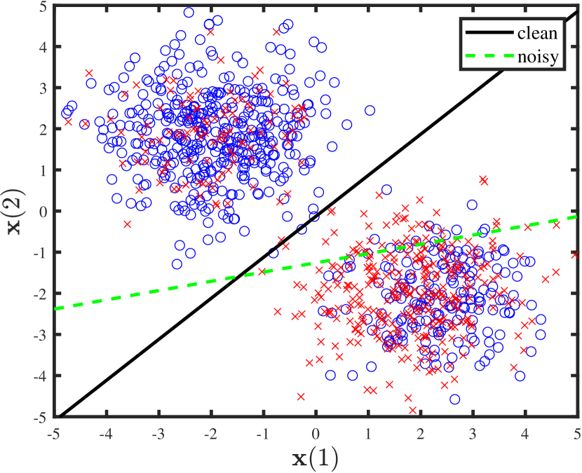
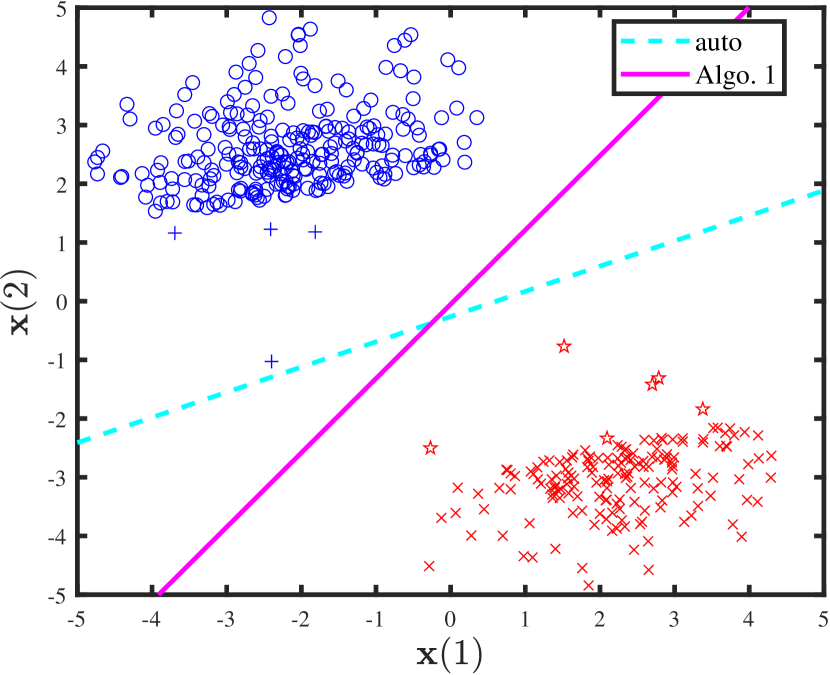
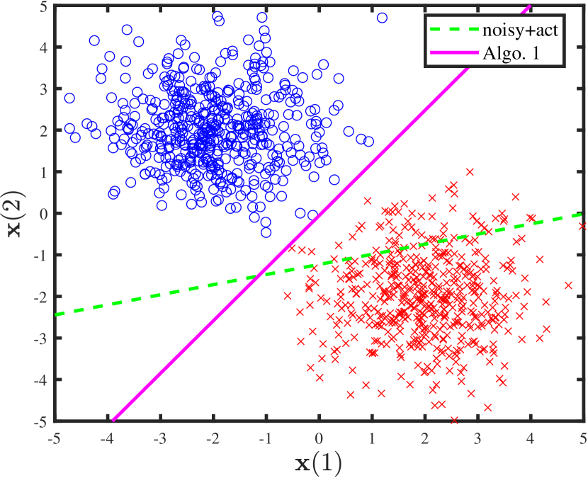
Figure 1: Visualization of the procedure of our Algorithm 1 (best viewed in color). In this trial, ($\rho_{\text{+1max}}$, $\rho_{\text{-1max}}$, $n_{\text{act}}$)=(0.25, 0.49, 10) and $\mathbf{w}_{+1}=[-0.2723,-0.8796,0.4133]^{\top}$, $\mathbf{w}_{-1}=[-0.6758,1.3259,0.1472]^{\top}$. 1: The noisy sample consisting of examples with noisy labels $+1$/$-1$ (blue circles/red x-marks) and the classification boundaries. 1: Our training sample consisting of automatically-collected positive/negative examples (blue circles/red x-marks) and actively-labeled positive/negative examples (blue plus/red pentagrams). Observe that most of automatically-collected distilled examples are correctly collected. 1: A contour plot showing distilled examples’ importance $\beta$, in which warmer color indicates greater importance. It demonstrates that actively-labeled examples are given greater importance than automatically-collected distilled examples, which is consistent with our analysis. 1: The test sample and classification boundaries.

Evaluations of our algorithm are conducted on both synthetic and real-world datasets. In our experiments, logistic regression is used for both training $\hat{f}$ and estimating $\tilde{\eta}$. For KMM, we always use the Gaussian kernel $k(\mathbf{x}_{i},\mathbf{x}_{j})=\exp(-\sigma\|\mathbf{x}_{i}-\mathbf{x}_{j}\|^{2})$ and the value of $\sigma$ is set as $\sigma=1$ for evaluations on synthetic datasets and $\sigma=0.01$ for evaluations on real-world datasets. The setup of parameters $\epsilon$ and $B$ is the same as that of Huang et al. (2007), i.e., $\epsilon=(\sqrt{m}-1)/\sqrt{m}$ and $B=1000$. In this section, each entry in the tables is the result averaged over 1000 trials.

4.1 The Case Where $\rho_{\text{+1max}}$ and $\rho_{\text{-1max}}$ Are Known

In this subsection, $\rho_{\text{+1max}}$ and $\rho_{\text{-1max}}$ are assumed to be known, and the evaluated methods are as follows:

1. “clean”: Train the classifier with clean examples.

2. “noisy”: Train the classifier with noisy examples.

3. “auto”: Train the classifier with automatically-collected distilled examples.

4. “auto+act”: Train the classifier with automatically-collected and manually-labeled distilled examples without importance reweighting. This can be viewed as a simplified version of our Algorithm 1.

5. “Algo. 1”: Train the classifier by our Algorithm 1.

6. “noisy+act”: Add the $n_{\text{act}}$ examples actively-labeled by “auto+act” into the noisy training sample and remove the corresponding noisy ones, and then train the classifier.

Note that “noisy+act” is used as a baseline for comparisons with our “auto+act”. The share of actively-labeled examples is to make comparisons fair.

4.1.1 Evaluations on Synthetic Datasets

Table 1: Means and Standard Deviations (Percentage) of Classification Accuracies of Different Classifiers

dataset	($\rho_{\text{+1max}}$, $\rho_{\text{-1max}}$,$n_{\text{act}}$ )	clean	noisy	auto	noisy+act	auto+act (ours)	Algo. 1 (ours)
Synthetic Dataset	(0.25, 0.25, 3)	99.73$\pm$0.17	98.55$\pm$1.28	99.13$\pm$0.83	98.56$\pm$1.27	99.28$\pm$0.70	99.30$\pm$0.68
	(0, 0.49, 3)		90.06$\pm$9.43	97.42$\pm$2.75	90.06$\pm$9.43	97.75$\pm$2.38	98.01$\pm$2.10
	(0.25, 0.49, 3)		92.59$\pm$8.64	97.95$\pm$2.70	92.60$\pm$8.63	98.69$\pm$1.67	98.90$\pm$1.37
	(0.49, 0.49, 3)		88.57$\pm$10.74	89.52$\pm$18.96	88.74$\pm$10.60	98.16$\pm$2.57	98.43$\pm$2.29
UCI Image	(0.1, 0.3, 20)	83.10$\pm$1.36	81.16$\pm$2.21	81.39 $\pm$1.83	81.15$\pm$2.21	81.78$\pm$1.72	82.09$\pm$1.71
	(0.3, 0.1, 20)		78.88$\pm$3.07	79.82$\pm$2.76	79.09$\pm$2.99	80.69$\pm$2.47	81.60$\pm$2.15
	(0.2, 0.4, 20)		78.94$\pm$3.10	77.96$\pm$3.16	78.98$\pm$3.12	79.46$\pm$2.72	81.08$\pm$2.32
	(0.4, 0.2, 20)		75.80$\pm$4.08	76.30$\pm$3.67	76.14$\pm$3.96	78.44$\pm$3.37	80.35$\pm$2.70
	(0.3, 0.3, 20)		79.02$\pm$2.90	77.48$\pm$3.23	79.21$\pm$2.82	79.16$\pm$2.88	80.97$\pm$2.34
	(0.4, 0.4, 20)		74.72$\pm$4.06	71.86$\pm$5.22	75.03$\pm$3.97	76.27$\pm$4.11	78.31$\pm$3.63
	(0.5, 0.5, 20)		68.72$\pm$5.91	64.49$\pm$7.39	69.19$\pm$5.80	73.64$\pm$4.95	75.64$\pm$4.69
USPS (6vs8)	(0.1, 0.3, 20)	98.07$\pm$0.52	89.00$\pm$1.84	93.55$\pm$1.47	89.01$\pm$1.82	93.72$\pm$1.43	93.74$\pm$1.44
	(0.3, 0.1, 20)		89.15$\pm$1.78	93.64$\pm$1.50	89.30$\pm$1.77	93.82$\pm$1.41	93.83$\pm$1.44
	(0.2, 0.4, 20)		86.40$\pm$2.31	91.45$\pm$1.91	86.46$\pm$2.31	91.65$\pm$1.85	91.67$\pm$1.86
	(0.4, 0.2, 20)		86.45$\pm$2.27	91.51$\pm$1.92	86.67$\pm$2.20	91.74$\pm$1.86	91.77$\pm$1.88
	(0.3, 0.3, 20)		87.01$\pm$2.13	91.74$\pm$1.83	87.15$\pm$2.08	91.97$\pm$1.73	91.98$\pm$1.77
	(0.4, 0.4, 20)		82.84$\pm$2.81	87.77$\pm$2.74	83.08$\pm$2.77	88.36$\pm$2.55	88.31$\pm$2.60
	(0.5, 0.5, 20)		77.73$\pm$3.96	82.22$\pm$4.20	78.06$\pm$3.88	83.35$\pm$3.90	83.19$\pm$3.92

First, we perform evaluations on 2D synthetic datasets that are linearly inseparable.

In each trial, positive examples and negative examples are sampled from two 2D normal distributions $\mathcal{N}_{1}(\mathbf{u},\mathbf{I})$ and $\mathcal{N}_{2}(-\mathbf{u},\mathbf{I})$ respectively, where $\mathbf{u}=[-2,2]^{\top}$ and $\mathbf{I}\in\mathbb{R}^{2\times 2}$ is the identity matrix. Each 2D datapoint $\left(\mathbf{x}(1),\mathbf{x}(2)\right)$’s feature vector is $[1,\mathbf{x}(1),\mathbf{x}(2)]^{\top}$ where $1$ act as an intercept term. We generate bounded instance- and label-dependent label noise at random via

$$\left\{\begin{aligned} \rho_{+1}(\mathbf{x})=\rho_{+1\text{max}}\cdot S\left(\mathbf{w}_{+1}^{\top}\mathbf{x}\right),\\ \rho_{-1}(\mathbf{x})=\rho_{-1\text{max}}\cdot S\left(\mathbf{w}_{-1}^{\top}\mathbf{x}\right),\\ \end{aligned}\right.$$ (4)

where elements of $\mathbf{w}_{+1},\mathbf{w}_{-1}$ are i.i.d. sampled from the standard normal distribution in each trial and $S(\cdot)$ denotes the sigmoid function $S(x)=\frac{1}{1+\exp{(-x)}}$.

The performances of evaluated methods under different ($\rho_{\text{{+1max}}}$, $\rho_{\text{{-1max}}}$, $n_{\text{act}}$) are shown in Table 1. Note that the standard deviations of some results are large, since in different trials label noise is generated by different noise rates functions. It is shown that our “auto+act” does not only always significantly outperform the baseline in terms of average classification accuracies, but also achieves smaller standard deviations compared to “noisy” and “noisy+act”.

The procedure of Algorithm 1 is visualized in Fig. 1.

Table 2: Means and Standard Deviations (Percentage) of Classification Accuracies of Different Classifiers

dataset	$\left(\rho_{\text{+1max}},\rho_{\text{-1max}},n_{\text{act}}\right)$	auto w/o $\rho_{\text{$\pm$1max}}$	noisy+act w/o $\rho_{\text{$\pm$1max}}$	Algo. 1 w/o $\rho_{\text{$\pm$1max}}$
Synthetic Dataset	(0.25, 0.25, 3)	99.54$\pm$0.31	98.62$\pm$1.25	99.61$\pm$0.33
	(0, 0.49, 3)	98.20$\pm$1.35	89.67$\pm$9.67	99.16$\pm$0.72
	(0.25, 0.49, 3)	99.10$\pm$2.24	92.54$\pm$9.00	99.41$\pm$0.74
	(0.49, 0.49, 3)	92.36$\pm$19.09	89.10$\pm$9.62	99.23$\pm$1.02
UCI Image	(0.1, 0.3, 20)	78.65$\pm$2.64	81.19$\pm$2.16	81.35$\pm$2.45
	(0.3, 0.1, 20)	75.00$\pm$3.84	79.25$\pm$3.06	80.38$\pm$2.85
	(0.2, 0.4, 20)	75.52$\pm$4.42	78.96$\pm$2.97	79.51$\pm$3.18
	(0.4, 0.2, 20)	71.38$\pm$5.03	76.26$\pm$3.79	78.63$\pm$3.56
	(0.3, 0.3, 20)	73.90$\pm$5.11	79.06$\pm$2.74	79.30$\pm$3.30
	(0.4, 0.4, 20)	69.20$\pm$5.64	75.01$\pm$3.78	76.85$\pm$4.52
	(0.5, 0.5, 20)	64.61$\pm$6.87	69.45$\pm$5.91	74.51$\pm$5.43
USPS (6vs8)	(0.1, 0.3, 20)	94.96$\pm$1.24	89.03$\pm$1.82	95.12$\pm$1.20
	(0.3, 0.1, 20)	95.02$\pm$1.28	89.34$\pm$1.79	95.15$\pm$1.26
	(0.2, 0.4, 20)	92.44$\pm$1.76	86.34$\pm$2.29	92.73$\pm$1.69
	(0.4, 0.2, 20	92.55$\pm$1.89	86.55$\pm$2.21	92.83$\pm$1.78
	(0.3, 0.3, 20)	93.15$\pm$1.69	87.03$\pm$1.95	93.46$\pm$1.63
	(0.4, 0.4, 20)	88.87$\pm$2.71	83.00$\pm$2.78	89.35$\pm$2.61
	(0.5, 0.5, 20)	82.52$\pm$4.06	77.95$\pm$3.86	83.40$\pm$3.87

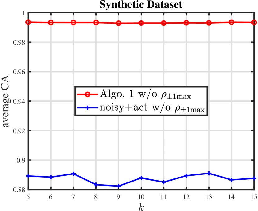
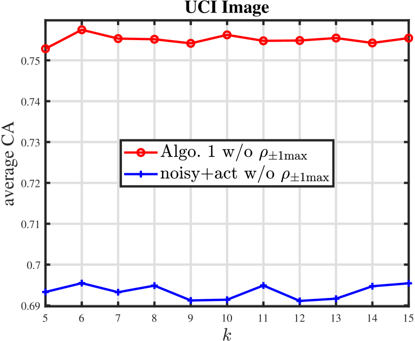
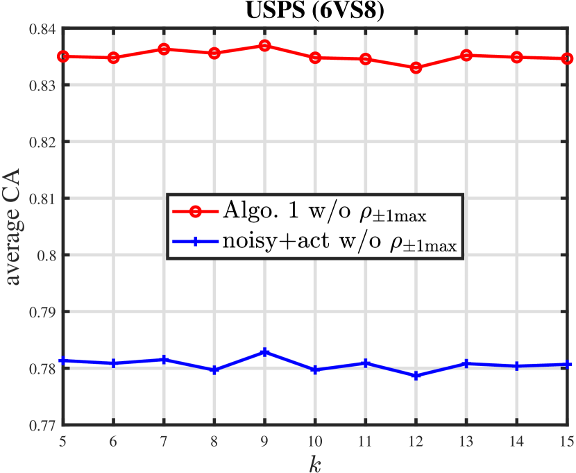
Figure 2: Curves illustrating the average classification accuracy (CA) of different classifiers learned without knowledge of $\rho_{+1\text{max}}$ and $\rho_{-1\text{max}}$ versus the hyperparameter $k$ on three datasets. The settings of ($\rho_{+1\text{max}}$, $\rho_{-1\text{max}},n_{\text{act}}$) in 2 and 2/2 are respectively (0.49, 0.49, 5) and (0.5, 0.5, 20). Each result in this figure is averaged over $1000$ trials.

4.1.2 Evaluations on Real-World Datasets

Second, we conduct evaluations on two public real-world datasets: the image dataset from the UCI repository provided by Gunnar Rätsch and the USPS handwritten digits dataset (Hull, 1994). The UCI Image dataset is composed of 1188 positive examples and 898 negative examples. As for the USPS dataset, We use images of “6” and “8” as positive and negative examples respectively, and each class has 1100 examples. In each trial, all feature vectors are standardized so that each element has roughly zero mean and unit variance, and examples are randomly split, $75\%$ for training and $25\%$ for testing. Label noise is generated in the same way with evaluations on synthetic datasets by Eq. (4).

Evaluation results are shown in Table 1. It is shown that our algorithm still outperforms the baselines.

4.2 The Case Where $\rho_{\text{+1max}}$ and $\rho_{\text{-1max}}$ Are Unknown

In this section, we evaluate variants of “auto”, “noisy+act” and “Algo. 1”, which employ the approach proposed in Sec. 3.5 to collect distilled example without knowledge of $\rho_{\pm 1\text{max}}$, on both synthetic and real-world datasets. The evaluated methods are denoted as “auto w/o $\rho_{\pm 1\text{max}}$”, “noisy+act w/o $\rho_{\pm 1\text{max}}$” and “Algo. 1 w/o $\rho_{\pm 1\text{max}}$”.

The setup of experiments is same with setup in Sec. 4.1. The only newly introduced hyperparameter is $k$. We set $k=10$ for all evaluations on three datasets, and avoid dataset specific tuning.

Results are listed in Table 2 and show that our “Algo. 1 w/o $\rho_{\pm 1\text{max}}$” outperforms the baseline. Comparing results in Table 2 and results in Sec. 4.1, we are surprised to observe that the performance of “Algo. 1 w/o $\rho_{\pm 1\text{max}}$” is comparable with and sometimes even better than that of “Algo. 1”.

To investigate the sensitivity of our algorithm to $k$, we plot the performance curves w.r.t. the variation of $k$ on three datasets in Fig. 2. It is shown that our algorithm is robust to the selection of $k$ on different datasets.

5 Conclusion

In this paper, we focus on learning with BILN, which is a more general case of label noise than those have been well-studied. We propose a learning algorithm and theoretically establish its statistical consistency and a performance bound. Empirical evaluations on synthetic and real-world datasets show effectiveness of the proposed algorithm.

In future, we will explore the combination of our algorithm and more complicated models (e.g., deep neural networks) for real-world label noise tasks.

References

- Angelova et al. (2005) Angelova, A., Abu-Mostafam, Y., and Perona, P. Pruning training sets for learning of object categories. In CVPR, 2005.
- Angluin & Laird (1988) Angluin, D. and Laird, P. Learning from noisy examples. Machine Learning, 2(4):343–370, 1988.
- Awasthi et al. (2015) Awasthi, P., Balcan, M.-F., Haghtalab, N., and Urner, R. Efficient learning of linear separators under bounded noise. In COLT, 2015.
- Awasthi et al. (2016) Awasthi, P., Balcan, M.-F., Haghtalab, N., and Zhang, H. Learning and 1-bit compressed sensing under asymmetric noise. In COLT, 2016.
- Bartlett & Mendelson (2002) Bartlett, P. L. and Mendelson, S. Rademacher and gaussian complexities: Risk bounds and structural results. Journal of Machine Learning Research (JMLR), 3(Nov):463–482, 2002.
- Bartlett et al. (2006) Bartlett, P. L., Jordan, M. I., and McAuliffe, J. D. Convexity, classification, and risk bounds. Journal of the American Statistical Association, 101(473):138–156, 2006.
- Blum & Mitchell (1998) Blum, A. and Mitchell, T. Combining labeled and unlabeled data with co-training. In COLT, 1998.
- Bootkrajang & Kaban (2012) Bootkrajang, J. and Kaban, A. Label-noise robust logistic regression and its applications. In ECML/PKDD, 2012.
- Bootkrajang & Kaban (2013) Bootkrajang, J. and Kaban, A. Boosting in the presence of label noise. In UAI, 2013.
- Brodley & Friedl (1999) Brodley, C. E. and Friedl, M. A. Identifying mislabeled training data. Journal of Artificial Intelligence Research (JAIR), 11(1):131–167, 1999.
- Bylander (1994) Bylander, T. Learning linear threshold functions in the presence of classification noise. In COLT, 1994.
- Chou et al. (2020) Chou, Y.-T., Niu, G., Lin, H.-T., and Sugiyama, M. Unbiased risk estimators can mislead: A case study of learning with complementary labels. In ICML, 2020.
- Diakonikolas et al. (2019) Diakonikolas, I., Gouleakis, T., and Tzamos, C. Distribution-independent pac learning of halfspaces with massart noise. arXiv preprint arXiv:1906.10075, 2019.
- Feng et al. (2020) Feng, L., Kaneko, T., Han, B., Niu, G., An, B., and Sugiyama, M. Learning with multiple complementary labels. In ICML, 2020.
- Fergus et al. (2010) Fergus, R., Fei-Fei, L., Perona, P., and Zisserman, A. Learning object categories from internet image searches. Proceedings of the IEEE, 98(8):1453–1466, 2010.
- Frénay & Verleysen (2014) Frénay, B. and Verleysen, M. Classification in the presence of label noise: A survey. IEEE Transactions on Neural Networks and Learning Systems (TNNLS), 25(5):845–869, 2014.
- Gao et al. (2016) Gao, W., Niu, X., and Zhou, Z. On the consistency of exact and approximate nearest neighbor with noisy data. arXiv: Learning, 2016.
- Ghosh et al. (2015) Ghosh, A., Manwani, N., and Sastry, P. Making risk minimization tolerant to label noise. Neurocomputing, 160:93–107, 2015.
- Ghosh et al. (2017) Ghosh, A., Kumar, H., and Sastry, P. Robust loss functions under label noise for deep neural networks. In AAAI, 2017.
- Goldberger & Ben-Reuven (2017) Goldberger, J. and Ben-Reuven, E. Training deep neural-networks using a noise adaptation layer. In ICLR, 2017.
- Han et al. (2018a) Han, B., Yao, J., Niu, G., Zhou, M., Tsang, I., Zhang, Y., and Sugiyama, M. Masking: A new perspective of noisy supervision. In NeurIPS, 2018a.
- Han et al. (2018b) Han, B., Yao, Q., Yu, X., Niu, G., Xu, M., Hu, W., Tsang, I., and Sugiyama, M. Co-teaching: Robust training of deep neural networks with extremely noisy labels. In NeurIPS, 2018b.
- Han et al. (2020) Han, B., Niu, G., Yu, X., Yao, Q., Xu, M., Tsang, I., and Sugiyama, M. Sigua: Forgetting may make learning with noisy labels more robust. In ICML, 2020.
- Han et al. (2019) Han, J., Luo, P., and Wang, X. Deep self-learning from noisy labels. In ICCV, 2019.
- Hendrycks et al. (2018) Hendrycks, D., Mazeika, M., Wilson, D., and Gimpel, K. Using trusted data to train deep networks on labels corrupted by severe noise. In NeurIPS, 2018.
- Hu et al. (2020) Hu, W., Li, Z., and Yu, D. Simple and effective regularization methods for training on noisily labeled data with generalization guarantee. In ICLR, 2020.
- Huang et al. (2007) Huang, J., Gretton, A., Borgwardt, K. M., Schölkopf, B., and Smola, A. J. Correcting sample selection bias by unlabeled data. In NeurIPS, 2007.
- Huang et al. (2019) Huang, J., Qu, L., Jia, R., and Zhao, B. O2u-net: A simple noisy label detection approach for deep neural networks. In ICCV, 2019.
- Hull (1994) Hull, J. J. A database for handwritten text recognition research. IEEE Transactions on pattern analysis and machine intelligence (TPAMI), 16(5):550–554, 1994.
- Ishida et al. (2017) Ishida, T., Niu, G., Hu, W., and Sugiyama, M. Learning from complementary labels. In NeurIPS, 2017.
- Jiang et al. (2018) Jiang, L., Zhou, Z., Leung, T., Li, L.-J., and Fei-Fei, L. Mentornet: Learning data-driven curriculum for very deep neural networks on corrupted labels. In ICML, 2018.
- Jin et al. (2003) Jin, R., Liu, Y., Si, L., Carbonell, J. G., and Hauptmann, A. G. A new boosting algorithm using input-dependent regularizer. In ICML, 2003.
- Kearns (1998) Kearns, M. J. Efficient noise-tolerant learning from statistical queries. Journal of the ACM, 45(6):983–1006, 1998.
- Khardon & Wachman (2007) Khardon, R. and Wachman, G. Noise tolerant variants of the perceptron algorithm. Journal of Machine Learning Research (JMLR), 8:227–248, 2007.
- Kim et al. (2019) Kim, Y., Yim, J., Yun, J., and Kim, J. Nlnl: Negative learning for noisy labels. In ICCV, 2019.
- Lang et al. (2016) Lang, T., Flachsenberg, F., von Luxburg, U., and Rarey, M. Feasibility of active machine learning for multiclass compound classification. Journal of Chemical Information and Modeling, 56(1):12–20, 2016.
- Lawrence & Scholkopf (2001) Lawrence, N. D. and Scholkopf, B. Estimating a kernel fisher discriminant in the presence of label noise. In ICML, 2001.
- Lee et al. (2018) Lee, K.-H., He, X., Zhang, L., and Yang, L. Cleannet: Transfer learning for scalable image classifier training with label noise. In CVPR, 2018.
- Li et al. (2019) Li, J., Wong, Y., Zhao, Q., and Kankanhalli, M. S. Learning to learn from noisy labeled data. In CVPR, 2019.
- Li et al. (2020) Li, J., Socher, R., and Hoi, S. C. Dividemix: Learning with noisy labels as semi-supervised learning. In ICLR, 2020.
- Li et al. (2017) Li, Y., Yang, J., Song, Y., Cao, L., Luo, J., and Li, L.-J. Learning from noisy labels with distillation. In ICCV, 2017.
- Liu & Tao (2016) Liu, T. and Tao, D. Classification with noisy labels by importance reweighting. IEEE Transactions on Pattern Analysis and Machine Intelligence (TPAMI), 38(3):447–461, 2016.
- Liu & Guo (2020) Liu, Y. and Guo, H. Peer loss functions: Learning from noisy labels without knowing noise rates. In ICML, 2020.
- Long & Servedio (2010) Long, P. M. and Servedio, R. A. Random classification noise defeats all convex potential boosters. Machine learning, 78(3):287–304, 2010.
- Ma et al. (2018) Ma, X., Wang, Y., Houle, M. E., Zhou, S., Erfani, S. M., Xia, S.-T., Wijewickrema, S., and Bailey, J. Dimensionality-driven learning with noisy labels. In ICML, 2018.
- Malach & Shalev-Shwartz (2017) Malach, E. and Shalev-Shwartz, S. Decoupling” when to update” from” how to update”. In NeurIPS, 2017.
- Massart & Nédélec (2006) Massart, P. and Nédélec, É. Risk bounds for statistical learning. The Annals of Statistics, 34(5):2326–2366, 2006.
- Menon et al. (2015) Menon, A. K., Rooyen, B. V., Ong, C. S., and Williamson, R. C. Learning from corrupted binary labels via class-probability estimation. In ICML, 2015.
- Menon et al. (2018) Menon, A. K., van Rooyen, B., and Natarajan, N. Learning from binary labels with instance-dependent noise. Machine Learning, 107(8-10):1561–1595, 2018.
- Natarajan et al. (2013) Natarajan, N., Dhillon, I. S., Ravikumar, P. K., and Tewari, A. Learning with noisy labels. In NeurIPS, 2013.
- Nguyen et al. (2020) Nguyen, D. T., Mummadi, C. K., Ngo, T. P. N., Nguyen, T. H. P., Beggel, L., and Brox, T. Self: Learning to filter noisy labels with self-ensembling. In ICLR, 2020.
- Northcutt et al. (2017) Northcutt, C. G., Wu, T., and Chuang, I. L. Learning with confident examples: Rank pruning for robust classification with noisy labels. In UAI, 2017.
- Patrini et al. (2016) Patrini, G., Nielsen, F., Nock, R., and Carioni, M. Loss factorization, weakly supervised learning and label noise robustness. In ICML, 2016.
- Patrini et al. (2017) Patrini, G., Rozza, A., Menon, A. K., Nock, R., and Qu, L. Making deep neural networks robust to label noise: A loss correction approach. In CVPR, 2017.
- Ramaswamy et al. (2016) Ramaswamy, H., Scott, C., and Tewari, A. Mixture proportion estimation via kernel embeddings of distributions. In ICML, 2016.
- Ren et al. (2018) Ren, M., Zeng, W., Yang, B., and Urtasun, R. Learning to reweight examples for robust deep learning. In ICML, 2018.
- Schroff et al. (2011) Schroff, F., Criminisi, A., and Zisserman, A. Harvesting image databases from the web. IEEE Transactions on Pattern Analysis and Machine Intelligence (TPAMI), 33(4):754–766, 2011.
- Scott (2015) Scott, C. A rate of convergence for mixture proportion estimation, with application to learning from noisy labels. In AISTATS, 2015.
- Scott et al. (2012) Scott, C. et al. Calibrated asymmetric surrogate losses. Electronic Journal of Statistics, 6:958–992, 2012.
- Seo et al. (2019) Seo, P. H., Kim, G., and Han, B. Combinatorial inference against label noise. In Advances in Neural Information Processing Systems, pp. 1171–1181, 2019.
- Settles (2010) Settles, B. Active learning literature survey. University of Wisconsin, Madison, 52(55-66):11, 2010.
- Tanaka et al. (2018) Tanaka, D., Ikami, D., Yamasaki, T., and Aizawa, K. Joint optimization framework for learning with noisy labels. In CVPR, 2018.
- Tong & Koller (2001) Tong, S. and Koller, D. Support vector machine active learning with applications to text classification. Journal of Machine Learning Research (JMLR), 2(Nov):45–66, 2001.
- Vahdat (2017) Vahdat, A. Toward robustness against label noise in training deep discriminative neural networks. In NeurIPS, 2017.
- van Rooyen et al. (2015) van Rooyen, B., Menon, A., and Williamson, R. C. Learning with symmetric label noise: The importance of being unhinged. In NeurIPS, 2015.
- Wang et al. (2018) Wang, Y., Liu, W., Ma, X., Bailey, J., Zha, H., Song, L., and Xia, S.-T. Iterative learning with open-set noisy labels. In CVPR, 2018.
- Wang et al. (2019) Wang, Y., Ma, X., Chen, Z., Luo, Y., Yi, J., and Bailey, J. Symmetric cross entropy for robust learning with noisy labels. In ICCV, 2019.
- Wu et al. (2020) Wu, S., Xia, X., Liu, T., Han, B., Gong, M., Wang, N., Liu, H., and Niu, G. Class2simi: A new perspective on learning with label noise. arXiv preprint arXiv:2006.07831, 2020.
- Xia et al. (2019) Xia, X., Liu, T., Wang, N., Han, B., Gong, C., Niu, G., and Sugiyama, M. Are anchor points really indispensable in label-noise learning? In NeurIPS, 2019.
- Xia et al. (2020) Xia, X., Liu, T., Han, B., Wang, N., Gong, M., Liu, H., Niu, G., Tao, D., and Sugiyama, M. Parts-dependent label noise: Towards instance-dependent label noise. arXiv preprint arXiv:2006.07836, 2020.
- Xiao et al. (2015) Xiao, T., Xia, T., Yang, Y., Huang, C., and Wang, X. Learning from massive noisy labeled data for image classification. In CVPR, 2015.
- Xu et al. (2019) Xu, Y., Cao, P., Kong, Y., and Wang, Y. L_dmi: A novel information-theoretic loss function for training deep nets robust to label noise. In NeurIPS, 2019.
- Xu et al. (2020) Xu, Y., Gong, M., Chen, J., Liu, T., Zhang, K., and Batmanghelich, K. Generative-discriminative complementary learning. In AAAI, 2020.
- Yan & Zhang (2017) Yan, S. and Zhang, C. Revisiting perceptron: Efficient and label-optimal learning of halfspaces. In NeurIPS, 2017.
- Yao et al. (2020) Yao, Q., Yang, H., Han, B., Niu, G., and Kwok, J. Searching to exploit memorization effect in learning from noisy labels. In ICML, 2020.
- Yi & Wu (2019) Yi, K. and Wu, J. Probabilistic end-to-end noise correction for learning with noisy labels. In CVPR, 2019.
- Yu et al. (2018) Yu, X., Liu, T., Gong, M., and Tao, D. Learning with biased complementary labels. In ECCV, 2018.
- Yu et al. (2020) Yu, X., Liu, T., Gong, M., Zhang, K., Batmanghelich, K., and Tao, D. Label-noise robust domain adaptation. In ICML, 2020.
- Zhang et al. (2017) Zhang, Y., Liang, P., and Charikar, M. A hitting time analysis of stochastic gradient langevin dynamics. In COLT, 2017.
- Zhang & Sabuncu (2018) Zhang, Z. and Sabuncu, M. R. Generalized cross entropy loss for training deep neural networks with noisy labels. In NeurIPS, 2018.
- Zheng et al. (2020) Zheng, S., Wu, P., Goswami, A., Goswami, M., Metaxas, D., and Chen, C. Error-bounded correction of noisy labels. In ICML, 2020.
- Zhu et al. (2003) Zhu, X., Wu, X., and Chen, Q. Eliminating class noise in large datasets. In ICML, 2003.