Analysing and Understanding Parallel Speedups

Techniques for Empirical Analysis of Memory Effects in Parallel Programs

Parallel Work Inflation, Memory Effects, and their Empirical Analysis

Abstract

In this paper, we propose an empirical method for evaluating the performance of parallel code. Our method is based on a simple idea that is surprisingly effective in helping to identify causes of poor performance, such as high parallelization overheads, lack of adequate parallelism, and memory effects. Our method relies on only the measurement of the run time of a baseline sequential program, the run time of the parallel program, the single-processor run time of the parallel program, and the total amount of time processors spend idle, waiting for work.

In our proposed approach, we establish an equality between the observed parallel speedups and three terms that we call parallel work, idle time, and work-inflation, where all terms except work inflation can be measured empirically, with precision. We then use the equality to calculate the difficult-to-measure work-inflation term, which includes increased communication costs and memory effects due to parallel execution. By isolating the main factors of poor performance, our method enables the programmer to assign blame to certain properties of the code, such as parallel grain size, amount of parallelism, and memory usage.

We present a mathematical model, inspired by the work-span model, that enables us to justify the interpretation of our measurements. We also introduce a method to help the programmer to visualize both the relative impact of the various causes of poor performance and the scaling trends in the causes of poor performance. Our method fits in a sweet spot in between state-of-the-art profiling and visualization tools. We illustrate our method by several empirical studies and we describe a few experiments that emphasize the care that is required to accurately interpret speedup plots.

1 Introduction

In the current state of the art, implementing a parallel algorithm on a multicore machine requires more than translating the algorithm to a parallel program by using a language or a parallelism API, such as OpenMP openmp , TBB ThreadingBuildingBlocksManual , X10 x10-2005 , or Cilk Plus IntelCilkPlus . During the development cycle, the programmer will likely have to tune their implementation by experimenting with several important parameters and optimizations in order to elicit decent performance. To this end, the programmer typically compares the performance of the parallel code with multiple processors to the performance of a sequential baseline and computes the speedup achieved as the ratio of the time for the baseline to the time for the multiprocessor run. It is well known that, for this comparison to be meaningful, the baseline has to be selected carefully and must be an optimal sequential algorithm and an optimized implementation.

After an initial implementation, speedup curves that the programmer obtains usually resemble those that are shown in Figure 1. Three of the speedup curves are taken from runs of three different configurations of the Cilksort benchmark  FrigoLeRa98 , and the other speedup is taken from one run of the Maximal Independent Set benchmark Blelloch:2012:IDP:2145816.2145840 . These speedups scale poorly, deviating significantly from the linear optimum. Faced with such results, the programmer has to study the performance of the code to identify and eliminate causes of suboptimal performance.

There are four main non-overlapping factors that contribute to suboptimal parallel performance.

• Algorithmic overheads, which correspond to the difference in the amount of work performed by the sequential baseline program and the sequential execution of the parallel program.

• Scheduling overheads, which consists of the cost of creating threads plus the cost of performing load balancing.

• Lack of parallelism in the application, that leads to idling processors which are starving for work.

• Work inflation, which we define as the increase in the cost of the operations performed in a parallel run compared with a single-processor run, when executing the parallel code.

Note that the first and the last factors are different. On the one hand, algorithmic overheads result primarily from the fact that a parallel algorithm is usually more complex than a sequential algorithm for the same problem. On the other hand, work inflation measures the increase in the work of the parallel implementation as we increase the number of processors. Work inflation includes memory subsystem effects, and the costs for communication, synchronization such as memory fences and atomic operations, false sharing, maintenance of cache coherency, contention at the memory bus, and memory consistency protocol. Because work inflation occurs at the hardware level, the overall impact of work inflation is difficult, if not impossible, to measure directly.

A key step in the tuning process is that of identifying which of the four factors are significant. For example, as we will see, each of the speedup curves in Figure 1 is poor due to just one or two of the four factors. By just looking at the speedup curves, it is not possible to determine which factors harm scalability and by how much. In general, despite their ability to show scaling trends, speedup curves can, by themselves, provide only vague hints into what factors harm scalability.

Although there are several performance tools to analyze parallel applications, there are currently neither tools nor widely-known methods that enable programmers to analyze the relative impact on scalability of the different factors, such as those listed above. The Cilkview analyzer can be used to predict the scalability of an application based on the logical parallelism expressed in control structure of the code HeLeiserson10 . However, if the code expresses plenty of parallelism, Cilkview analyzer is unlikely to provide additional insights into the causes of poor performance. Tools such as Intel Thread Profiler IntelParallelAdvisor , Intel Parallel Amplifier IntelParallelAmplifier , HPCToolkit TallentMellorCrummey07 , Kismet JeonGarciaLouie11 and Kremlim GarciaJeonDonghwan11 can provide detailed information on the utilization of the processors over time and on the breakdown of the relative importance of the subroutines of the program. Predator LiuBergerPredator can detect false sharing in instrumented runs of application code. Each of these tools fills an important gap in the toolkit of a parallel programmer. Nevertheless, none of these tools are suitable for analyzing all types of performance issues.

A separate issue relates to profiling instrumentation. Cilkview relies on binary instrumentation and analyzes only instruction counts. The other tools rely on various other forms of instrumentation. Such instrumentation increases the risk that instrumentation-specific overheads will themselves influence performance, and the overheads will do so in ways that obscure the performance issues of interest. Although it is sometimes essential to understand certain aspects of performance, heavyweight instrumentation causes interference that can obscure the global picture, that is, the performance of the production binary, which typically has little or no instrumentation.

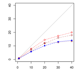
Figure 1: Traditional speedup curve showing four poor speedups. The y axis represents the speedup and the x axis the number of processors.

In this paper, we present an experimental method for diagnosing observed performance and scalability problems. Our proposal rests on some simple observations but it provides a surprisingly effictive and non-intrusive approach.

Our approach relies on the following measurements:

• the sequential execution time of the baseline program,

• the sequential execution time of the parallel program (i.e., the running time of the parallel program using a single processor),

• the parallel execution time of the parallel program (with different numbers of cores),

• the total time that processors spend idling (waiting for work).

Using these measures, we show that it is possible to derive the amount of work inflation, a quantity that is difficult to measure directly. More generally, we are able to calculate the amount of speedups lost due to overheads associated with the parallel algorithm, the amount of speedups lost due to idle time, and the amount of speedups lost due to the work inflation. By measuring and calculating these values for various number of processors, we can study scalability trends, and the factors contributing the observed results. As we describe (§2.1), these quantities can be measured unintrusively, without heavy instrumentation of the binary, and are therefore representative of the actual, observed performance (they are not based on simulations or profiling information).

Using such measurements, we propose an approach to visulazing important performance information in the form of factored speedup plots that include three additional speedup curves, all of which are calculated with respect to the optimized sequential baseline. These plots enable studying the different contributing factors to the speedups.

• A maximal speedup plot shows the speedups that the program would obtain if we ignore work inflation and idle time. In other words, the maximal speedup plot shows the speedups that would be achieved if the speedup of the parallel program were scaling up linearly with the number of processors.

• An idle-time-specific speedup plot takes into account idle time but ignores work inflation. In other words, idle-time-specific speedups represent the speedups that would be obtained if only the idle time and algorithmic overheads (the overheads of the parallel program with respect to the baseline) were preventing the program from achieving maximal speedups.

• An inflation-specific speedup plot shows the speedups that the program would obtain if we ignore idle time. In other words, the inflation-specific speedup represents the speedup that would be achieved if only the work inflation and the algorithmic overheads were preventing the program from achieving maximal speedups.

Figure 2 shows the factored speedup curves for the Cilksort benchmark with one specific configuration. Our factored speedup plot enables the programmer to visualize all three curves at once. The plot conveys three types of information: (1) the absolute position of the curves, (2) the relative position of the curves (i.e., the gaps between the curves), (3) the shapes of the curves (i.e., curvature), which informs on the scaling of specific speedup curves.

Workflow.

Our factored speedup plot plays a complementary role to the parallel-performance analyzers. If the factored speedup plot suggests lack of parallelism in the application, then the programmer may choose to find the bottleneck using a tool such as Cilkview. If the program is large and it is not clear which pieces of the code to blame for lack of parallelism, the programmer may search for the most significant regions of code using one of the tools, such as HPCToolkit and Kremlin. If work inflation is high, the programmer may choose to look for potential false sharing with Predator, for example. After a problematic region of code is identified, the programmer may synthesize from the region a smaller benchmark program and repeat the process from above.

Unlike many other other methods for analyzing performance of parallel codes, ours enables the programmer to observe their production code directly. As such, our method fits into a gap that we believe exists between traditional speedup plots and existing parallel performance tools, such as Cilkview. The close correspondence between the production binary and our lightweight profiling binary is possible thanks to the property that instrumentation we insert into the program has no noticable impact on the performance of the parallel code.

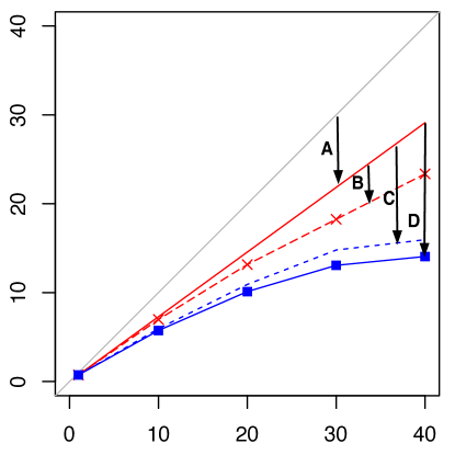
Figure 2: Factored speedup curves (top to bottom): linear, maximal, idle-time specific, inflation specific, and actual speedups for Cilksort. The arrows indicate gaps between the speedup curves that helps identify the contribution of each factor.

While developing algorithms and studying their efficiency with the help of factored speedup plots, we have often been impressed by how much work inflation (and thus speedups) could be affected, in counterintuitive ways, by the degree of optimization of the program code, and by the size of input data with respect to the size of the cache. In order to illustrate the extent to which speedups can be affected by these two aspects, we complete our paper with microbenchmark studies demonstrating how seemingly minor changes in the parameters can significantly affect the speedups measured.

Our contributions are as follows.

• We present a model, inspired by the work-span model, which accounts for work inflation, even though work inflation cannot be predicted by any theory and cannot be measured directly.

• We introduce factored speedup plots as a practical technique for visualizing the relative contribution of each of the three main sources of slowdown considered by our model: overheads, idle time and work inflation.

• We describe two artifacts that may significantly affect the interpretation of speedup curves. Although the existence of these effects is well know, we believe that the degree to which they can impact work inflation is often underappreciated.

2 A Method for Diagnosing Performance Problems

We describe a method for diagnosing problems with performance and scalability by identfying the contributions of the factors that mentioned in the introduction. For the purposes of mathematical simplicity, at first, we do not consider scheduling overheads, and we assume that our measurements (programs and schedulers) are deterministic. We later describe how to account for non-determinism (Section 2.7) and scheduling overheads (Section 2.8).

2.1 Measures

Given a parallel program, and given an associated sequential baseline program, our approach relies on the four following measures.

• $T_{s}$, the execution time of the sequential baseline.

• $T_{P}$, the execution time of the parallel program with $P$ cores.

• $I_{P}$, the total idle time associated with the parallel program (measured by instrumenting the scheduler).

• $T_{1}$, the 1-core execution time of the parallel program. We call $T_{1}$ the “parallel work with 1 core”.

Measuring $T_{s}$, $T_{P}$ and $T_{1}$ is achieved by querying the system time at the beginning and at the end of the executions. In particular, it does not require any instrumentation of the code being benchmarked. Measuring $I_{P}$ is just slightly more complex. We measure the total idle time by instrumenting the main loop of the scheduler code that is executed by each core, and which handles load balancing operations. We compute for each core the sum of the duration of the periods of time during which the core is waiting to acquire work. We call such periods idle phases, and we measure their duration using unobtrusive cycle-counter instructions, which are provided by modern multicore machines.

The total cost of our instrumentation of the scheduler is negligible in front of the execution time of the program. For each idle phase, we perform two queries to the cycle counters, and update one field from the thread-local storage. To end an idle phase, the processor needs to receive at least one task, and the time required to complete the execution of this task is in general a lot greater than the cost of measuring the duration of the idle phase.

Moreover, when a work-stealing scheduler is used, the total number of idle phases is relatively small. More precisely, the number of idle phases is bounded by $P-1$ plus the number of steals, because initially all cores are idle but one, and each idle phase can only end as a result of a successful steal. Analysis of work stealing shows that, for all programs that exhibit sufficient parallelism, the number of steals is, with high probability; relatively small in front of the total number of tasks acarchra13 . In summary, the overhead of our instrumentation is, for all practical purposes, negligible in front of the total execution time.

2.2 Definitions

Using the four measurements stated above, we derive two additional quantities.

• $W_{P}$, the parallel work with $P$ cores.

• $F_{P}$, the work inflation with $P$ cores.

To see how to calculate these additional quantities, we start with a simple fact.

Fact 2.1 (time decomposition).

The total amount of time available to the $P$ cores during a run that lasts $T_{P}$ time decomposes in work time and idle time.

$$P\cdot T_{P}\,=\,W_{P}+I_{P}.$$

This fact makes it immediately possible to calculate $W_{P}$.

Recall that we define work inflation to be the increase in work as a result of parallel execution. This leads to the following fact.

Fact 2.2 (definition of work inflation).

Work inflation (at $P$ cores) is the difference between the work performed by the parallel program when using $P$ cores and the work performed by the same program when using a single core. We therefore have:

$$F_{P}\,=\,W_{P}-T_{1}.$$

As shown by the fact below, we can calculate the work inflation $F_{P}$

Fact 2.3 (formula for work inflation).

$$F_{P}\,=\,P\cdot T_{P}-I_{P}-T_{1}.$$

For the purpose of analysing speedups (Section 2.3) and of comparison with the work-span model (Section 2.6), we combine the previous facts so as to obtain a reformulation of the parallel execution time in terms of the values of $T_{1}$ (1-core execution time of the parallel program), $I_{P}$ (idle time) and $F_{P}$ (work inflation).

Fact 2.4 (reformulation of parallel time).

The parallel execution time can be expressed as follows:

$$T_{P}\,=\,\frac{T_{1}+I_{P}+F_{P}}{P}.$$

2.3 Factored speedup plots

In order to better understand the effect of work inflation and idle time on the speedup values achieved by parallel programs, we reformulate, using Fact 2.4, the expression of speedup values, which is defined as the baseline time divided by the parallel time.

Fact 2.5 (reformulation of speedups).

The speedup at $P$ cores can be reformulated as follows:

$$\textsf{speedup}\,=\,\frac{T_{s}}{T_{P}}\,=\,\frac{P\cdot T_{s}}{T_{1}+I_{P}+F_{P}}$$

Starting with this formula, we propose four speedup measures that offer upper bounds of varying degrees of precision. Analyzing these speedups and the gaps between them we can determine the effects of work inflation and other characteristics of the computation on the performance.

Linear speedups.

When using $P$ cores to perform a computation, we generally do not expect the parallel execution to be more than $P$ times faster than the sequential baseline. Therefore, the linear speedup at $P$ cores is equal to the value $P$.

Maximal speedups.

We define the quantity

$$\frac{P\cdot T_{s}}{T_{1}}$$

as the maximal speedup because it assumes the work inflation and the idle time to be zero. Maximal speedups offer a realistic upper bound on the parallel speedup by taking into account the (possibly) additional work that must be performed by the parallel run in relation to the sequential run.

Idle-time-specific speedup.

We define the quantity

$$\frac{P\cdot T_{s}}{T_{1}+I_{P}}$$

as the idle-time-specific speedup because it assumes work inflation to be zero but takes into account available parallelism (as measured by the idle time).

Inflation-specific speedup.

We define the quantity

$$\frac{P\cdot T_{s}}{T_{1}+F_{P}}$$

as the inflation-specific speedup because it assumes idle time to be zero but takes into account work inflation. In the formula above, since we cannot measure $F_{P}$ directly, we deduce it from $T_{P}$ and $I_{P}$. More precisely, the inflation-specific speedup is computed as ${(P\cdot T_{s})}/{(P\cdot T_{P}-I_{P})}$.

Actual Speedups.

By definition, the actual speedup is:

$$\frac{T_{s}}{T_{P}}$$

2.4 Minding the gap

The three forms of speedups help analyze the empirical behavior of a parallel algorithm by isolating several different effects into different curves. Figure 2 shows an example. The linear speedup is drawn as the diagonal. Right below it is the maximal speedup, drawn with a solid black line.

The gap labelled A between the linear and the maximal speedups shows the amount of the algorithmic overheads that can be expected from parallelization and the overhead of thread creation. In other words, we can expect to match maximal speedups if the computation is fully parallel and only on parallel hardware that is able to support all operations with excellent scalability.

Right below the maximal speedup curve lies the idle-time-specific speedup curve, which takes into account the amount of parallelism but excludes work inflation. The gap labelled B between idle-time-specific speedup and the maximal speedup shows the idle time, which, assuming an close-to-greedy scheduler and a sufficiently-fine granularity of the tasks, reflects the scarcity of parallelism in the computation: the larger the gap, the scarcer is parallelism. We can expect to match idle-time-specific speedups only on parallel hardware that exhibits no noticable communication overheads and is able to scale memory operations well.

Right below the idle-time-specific speedup curve lies the inflation-specific speedup curve. The gap labelled C between the maximal speedup and the inflation-specific speedup illustrates the amount of work inflation: the larger the gap, the greater the work inflation.

At the bottom, the actual speedup curve reports on the speedups actually measured. The speedups include all measured factors (algorithmic overheads, idle-time, and work inflation. The gap labelled D illustrates the amount of speedup lost to idle time and work inflation combined. Finally, note that the gap between the actual speedup curve and idle-time-specific speedup curve indicates the amount of work inflation, and that the gap between the actual speedup curve and the inflation-specific curve speedup indicates the amount of idle time.

2.5 Minding the curvature

In addition to studying the space between the curves, it is often also possible to deduce useful information from the curvature of the curves. A few features are particularly informative.

If the maximal speedup curve is not a straight line but instead tends to flatten, then this curve indicates that the amount of overhead increases with the number of cores. In such case, the algorithm presumably would not scale up well with the number of cores.

Let us assume that the overhead curve appears as a straight line. If the idle-time-specific curve flattens towards a horizontal line, then this curve indicates that the additional computation time provided by using more cores is mostly wasted as idle time. Presumably, the program lacks parallelism.

If the inflation-specific curve flattens towards a horizontal line, then this curve indicates that the additional computation time provided by using more cores is almost entirely converted into work inflation. This situation is generally characteristic of a memory bottleneck that limits the throughtput of the operations performed on the main memory.

If the inflation-specific curve ends up slopping downwards, then this curve indicates that using more cores actually degrades the performance of the parallel program. This situation is typically caused by synchronization, in particular extensive use of either atomic operations or false sharing or both.

2.6 Work-span model versus inflation model

Comparing our proposed model with the work-span model brings out interesting similarities and differences between the two approaches. Consider a parallel program with work $T_{1}$ and span $T_{\infty}$, and whose parallel time is $T_{P}$ on $P$ processors. In the work span model (based on Brent’s theorem Brent74 , using a greedy scheduler), the parallel time, ignoring scheduling costs, is bounded as

$$T_{P}\,\leq\,\frac{T_{1}}{P}+T_{\infty}.$$

By comparison, our model does not provide an upper bound, but instead the following exact equality that involves (measured) idle time and (derivable) work inflation (Fact 2.4),

$$T_{P}\,=\,\frac{T_{1}}{P}+\frac{I_{P}}{P}+\frac{F_{P}}{P}.$$

If we ignore scheduling costs, then there are two important differences between the work-span model and our approach. First, our proposal relies on the measurement of the actual average amount of idle time per core (that is, ${I_{P}}/{P}$), rather than an upper bound computed as a property of the computation (that is, the span $T_{\infty}$). Second, our proposal includes a term for work inflation, whereas the work-span model does not account for differences between the uniprocessor work and multiprocessor work.

2.7 Generalization to non-deterministic executions

In this section, we justify that our approach naturally extends to non-deterministic executions. We call run a particular instance of a program execution. In particular, for a parallel execution, the run describes the schedule, that is, for each instruction, the time at which and the core on which it gets executed. We let $\mathcal{R}_{s}$ denote the set of runs of the sequential baseline, $\mathcal{R}_{P}$ the set of runs of the parallel program with $P$ cores, and $\mathcal{R}_{1}$ the set of runs of the parallel program with $1$ core. We let $R$ be a random variable ranging over one of these three sets of runs.

• Given a run $R$ in $\mathcal{R}_{s}$, we let $T_{s}(R)$ denote the execution time of this run.

• Given a run $R$ in $\mathcal{R}_{P}$, we let $T_{P}(R)$ denote the execution time of this run.

• Given a run $R$ in $\mathcal{R}_{P}$, we let $I_{P}(R)$ denote the total idle time involved in this run.

• Given a run $R$ in $\mathcal{R}_{1}$, we let $T_{1}(R)$ denote the execution time of this run.

We then define the parallel work of a run as follows:

$$W_{P}(R)\,\equiv\,P\cdot T_{P}(R)-I_{P}(R)$$

We define the work inflation of a run as the difference between the parallel work of this run and the expected work of a 1-core run. Regarding the latter, we write $\operatorname{\mathbb{E}}[T_{1}(R^{\prime})]$ the expected execution time of a random run $R^{\prime}$ in $\mathcal{R}_{1}$. The formal definition of work inflation is thus:

$$F_{P}(R)\,\equiv\,W_{P}(R)-\operatorname{\mathbb{E}}[T_{1}(R^{\prime})].$$

We write $T_{s}$ the expected value of $T_{s}(R)$, for $R$ in $\mathcal{R}_{s}$. Similary, we write $T_{P}$ and $I_{P}$ the expected values of $T_{P}(R)$ and $I_{P}(R)$, respectively, for $R$ in $\mathcal{R}_{P}$, and write $T_{1}$ the expected value of $T_{1}(R)$ for $R$ in $\mathcal{R}_{1}$. (Note that $T_{1}$ is the same as $\operatorname{\mathbb{E}}[T_{1}(R)]$.) With this notation, the earlier definitions given for the deterministic case can be applied without any modification. In particular, we define:

• Ideal speedup, as the value $P$.

• Maximal speedup, as the value $\frac{P\cdot T_{s}}{T_{1}}$.

• Idle-time-specific speedup, as the value $\frac{P\cdot T_{s}}{T_{1}+I_{P}}$.

• Inflation-specific speedup, as the value $\frac{P\cdot T_{s}}{P\cdot T_{P}-I_{P}}$.

• Actual speedup, as the value $\frac{T_{s}}{T_{P}}$.

Observe that, in the formulae above, we have chosen to compute the ratios of expected values, as opposed to the expected values of ratios. For example, we define actual speedup as $\frac{\operatorname{\mathbb{E}}[T_{s}(R)]}{\operatorname{\mathbb{E}}[T_{P}(R^{\prime})]}$ and not as $\operatorname{\mathbb{E}}[\frac{T_{s}(R)}{T_{P}(R^{\prime})}]$. The alternative choice would also be possible. However, we believe that, given a sample of measured runs, it makes more sense to report the speedup associated with the average execution time, rather than to report the average speedup value, because speedups are only a tool for analysing performance, whereas the execution time is what we ultimately care to minimize.

2.8 Accounting for scheduling costs

In this section, we explain how our approach smoothly generalizes to take scheduling costs into account. We start by introducing the following additional variables:

• $S_{1}$, the scheduling work of a 1-core run of the parallel program.

• $S_{P}$, the scheduling work of a P-core run of the parallel program.

• $W_{1}$, the user work of a 1-core the parallel program. We call “user work” the work performed by the user code as opposed to that performed by the scheduler.

• $W_{P}$, the computation work of a P-core the parallel program. Here, $W_{P}$ plays has the same role as before, but it explicitly excludes the scheduling work, which is no longer neglected.

Even though the 4 quantities above are hard to measure directly, we can use them to help us to provide valuable interpretation to the curves from factored speedup plots.

We define the scheduling work inflation, written $F_{P}^{\textsf{sched}}$, as the difference between the scheduling work performed by $P$ cores and that performed by a single core. Symmetrically, we define the user work inflation, written $F_{P}^{\textsf{user}}$, as the difference between the user work performed by $P$ cores and that performed by a single core. Finally, we define the work inflation to be the sum of the user work inflation and the scheduling work inflation.

$$\begin{array}[]{l@{\;\,}l@{\;\,}l}F_{P}^{\textsf{sched}}&{\equiv}&S_{P}-S_{1}\vspace{3pt}\\ F_{P}^{\textsf{user}}&{\equiv}&W_{P}-W_{1}\vspace{3pt}\\ F_{P}&{\equiv}&F_{P}^{\textsf{user}}+F_{P}^{\textsf{sched}}\end{array}$$

As we are going to establish next, the value of $F_{P}$, which denotes the total work inflation, can be computed from the same four measures as before. To prove it, we begin with two simple observations.

Fact 2.6 (decomposition of $1$-core execution times).

The execution time of $1$-core run of the parallel program decomposes as user work plus scheduling work.

$$T_{1}\,=\,W_{1}+S_{1}.$$

Fact 2.7 (decomposition of $P$-core execution times).

The execution time of a $P$-core run of the parallel program decomposes as user work, plus scheduling work, plus idle time.

$$P\cdot T_{P}\,=\,W_{P}+S_{P}+I_{P}.$$

Combining these two facts and the three definitions above shows that the total work inflation can be computed using exactly the same formula as before (recall Fact 2.3), when we ignored all scheduling costs.

Fact 2.8 (formula for work inflation, with scheduling costs).

$$F_{P}\,=\,P\cdot T_{P}-I_{P}-T_{1}.$$

When taking into account scheduling costs, we continue using exactly the same formulae for constructing factored speedup plots. Only the interpretation of these plots needs to be refined slightly.

• The 1-core work ($T_{1}$) now includes the scheduling work at 1-core ($S_{1}$). So, the maximal speedup curves includes not just the algorithmic overheads but also the scheduling work at 1-core.

• The idle-time specific is, as before, based on the maximal speedup, so it includes the scheduling work at 1-core.

• The inflation-specific speedup also includes the scheduling work, but also the scheduling work inflation. As we explain next, the scheduling work inflation is typically negligible.

When using a work stealing scheduler, the scheduling work inflation only includes the cost of performing load balancing and, if using concurrent deques, the possible increase in the cost of accessing the deques due to concurrent accesses to the same cache lines. For most practial applications, the number of steals is relatively small and the accesses to the deques are relatively cheap in front of the work performed by the threads, so the scheduling work inflation ($F_{P}^{\textsf{sched}}$) is negligible. In such a case, the work inflation ($F_{P}$) can be considered equivalent to the user work inflation ($F_{P}^{\textsf{user}}$).

As a concluding remark, we observe that the scheduling work at 1-core ($S_{1}$) can be estimated by running the sequential elision of the parallel program. This elision consists of a copy of the parallel code in which all parallelism constructs are replaced with sequential constructs. For example, fork-join operations are replaced with simple sequences. Let $T_{\textsf{elision}}$ denote the execution time of the sequential elision. We can estimate $S_{1}$ by considering the difference with the 1-core execution time of the parallel program. In other words, $S_{1}\,\approx\,T_{1}-T_{\textsf{elision}}$. When the sequential elision program is available, we can extend the factored speedup plot to report its execution time. To that end, we add an extra curve, located above the maximal speedup curve, showing the points at height: ${(P\cdot T_{s})}/{T_{\textsf{elision}}}$. This additional curve is useful in particular to easily spot issues related to granularity control, whereby the creation of too-small tasks imposes significant scheduling overheads. When granularity control is performed properly and an efficient scheduler is used, the new curve should collapse with that of maximal speedups, reflecting the fact that scheduling costs ($S_{1}$) are neglible.

3 Case studies

This section illustrates the application of our method on a multicore machine with several different runs of a few benchmark programs. We ported these programs from well-established benchmark suites, such as the Cilk benchmarks and the Problem Based Benchmark Suite, to our scheduling library. Although we selected only a few benchmark programs, we emphasize that the methods we use are readily applicable to any of the other benchmark programs in the respective suites and, more generally, to any Cilk program.

Experimental setup.

We conducted all the experiments described on our 40-core test machine. The machine hosts 4 Intel E7-4870 chips running at 2.4GHz and has 1Tb of RAM. Each chip has 10 cores and shares a 30Mb L3 cache. Each core has 256Kb of L2 cache and 32Kb of L1 cache, and hosts 2 SMT threads, giving a total of 80 hardware threads, but to avoid complications with hyperthreading we did not use more than 40 threads. The system runs Ubuntu Linux (kernel version 3.2.0-43-generic). We also ran the same experiments on a 48-core AMD machinewhich features a deeper memory hierarchy, and observed similar results. All our programs are implemented in C++, compiled with GCC 4.8, and rely on the scheduling library PASL, which itself relies on a work stealing scheduler. PASL provides two schedulers: one implemented with concurrent deques (like in Cilk), and another one implemented using private deques (see acarchra13 ). Both schedulers gave similar results on the benchmarks described in the present paper.

3.1 Case study 1: typical factored speedup plots

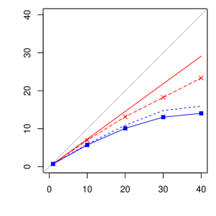
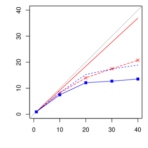
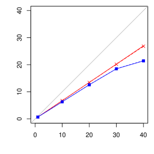
(a) small cutoff, small array	(b) very large cutoff, small array	(c) small cutoff, large array

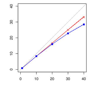
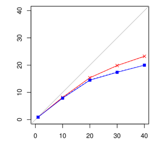
(d) large cutoff, large array	(e) large cutoff, huge array	(f) cutoff in $O(\frac{1}{P})$, large array

Figure 3: Case study 2: factored speedup curves for Cilksort benchmark. The straight, black curve represents the maximal speedup curve, the dotted, crossed one the idle-time specific curve, the dotted, blue one the inflation-specific curve, and the solid, blue one the actual speeedup curve.

To illustrate the utility of factored speedup plots in practice, we consider a classic benchmark program, namely Cilksort, and use factored speedup plots to analyze its performance. Cilksort sorts an array of 32-bit integers, using a variant of merge-sort that relies on a parallel merge operation, and relying on insertion-sort for sorting sub-arrays of 20 elements or fewer. When the input is smaller than a user specified cutoff, Cilksort reverts to sequential execution. Sequentialized sorting uses the quicksort algorithm. Quicksort is also used to measure the sequential baseline, used when computing speedup values.

In our experiment, we control the size of the input array, and the cutoff, to determine how Cilksort behaves under different settings. (We use the same cutoff for both the sort phase and the merge phase.) The goal of our experiments is to illustrate various typical type of factored speedup plots that one observe in practice.

In Chart (3.a), we consider a small array, containing 200k items, and a small cutoff, of 200 items. This chart indicates that our program suffers simultaneously from three problems: large parallel work as indicated by the gap between the linear and the maximal speedup curves, scarce parallelism as indicated by the gap between the maximal and the idle-time-specific speedup curves, and work inflation as indicated by the idle-time-specific and actual speedup curves.

In Chart (3.b), we attempt to reduce the thread-creation overheads by increasing the cutoff size to 10k items. The gap between the maximal speedup and the linear speedup closes indicating that we have successfully reduced parallel work. Actual speedups, however, have not improved—there are actually slightly worse—because parallelism reduced as indicated by the increased gap between the maximal and the idle-time-specific speedup curves. This suggests the cutoff is too large for this input, pinpointing exactly the source of the problem. Remark: the fact that the inflation-specific and idle-time-specific speedups are at about the same height indicates that both work inflation and idle time contribute to roughtly the same amount of lost speedups.

In Chart (3.c), we revert to the smaller cutoff of 200 items and try instead to address the lack of parallelism, by increasing the array size to 10 million items. The overheads in Chart (3.c) are similar to those of Chart (3.a), which is expected since we used the same cutoff value. The idle time has been reduced significantly, thanks to the increase in the amount of parallelism available. In this chart and the subsequent ones, the amount of idle time is negligible, so idle-specific curves collapse onto maximal speedup curves, and inflation-specific curves collapse onto actual speedup curves.

In Chart (3.d), we target a large array of 10m items and use a not-too-small cutoff of 1000 items. The chart reports decent speedups (28.5x at 40 cores), and the trend of the speedup curve suggests good scalability.

In Chart (3.e), we increase further the array size, up of 100m items, while keeping the same cutoff of 1000 items. The results are very similar to Chart (3.d), only with slightly better speedups (29.8x at 40 cores), showing that beyond a certain point, creating more parallelism no longer reduces the idle time. In fact, from the position of the overhead curve, which reaches 33.1x at 40 cores, we can deduce that, no matter the array size, it is highly unlikely to ever exceed a speedup of 33.1x on our test machine.

With Chart (3.f), we complete our case study with a last experiment which aims at illustrating a situation where the amount of work varies with the number of processors. To that end, we provide to Cilksort a cutoff inversely proportional to the number of processors. Note that adapting the number of subtasks generated to the number of processors is a classic technique, used for example in Cilk’s compilation of for-loops.

For this last experiment, we consider an array of size 10m and a cutoff of $8000/P$. As the value of $T_{1}$ actually depends on $P$, we write it $T_{1}^{P}$. To obtain the values of $T_{1}^{P}$, we perform, for each value of $P$, a single-processor run using the cutoff value $8000/P$. The results, shown in Chart (3.f), indicate that the idle time is negligible, that the memory effects are very limited, and that overheads are responsible for most of the lost speedups. Furthermore, on the chart we are able to observe the curvature of the overhead curve. The fact that the overhead curve is not a straight line but instead bends downwards indicates that the amount of overhead increases with the number of processors.

In summary, by looking at the curvature of the curves and the space between the curves of factored speedup plots, we are able to visualize, all at once, the relative contribution to the loss in speedups of each of the three possible sources of slowdown identified by our model, and also to visualize the trends of these contributions as the number of processors vary.

3.2 Case study 2: effect of NUMA allocation policies

We now describe how our factored speedup plot can be used to diagnose memory bottlenecks. For this study, we consider the Maximal Independent Set benchmark from the Problem Based Benchmark Suite. The maximal independent set problem is the following: given a connected undirected graph $G=(V,E)$ and find a subset of the vertices $U\subset V$ such that no vertices in $U$ are neighbors in $G$ and all vertices in $V\,\backslash\,U$ have a neighbor in $U$. For input to the benchark, we used the 2-d grid with $140$m vertices. For the baseline measurement, we use the sequential solution that is provided by the Problem Based Benchmark Suite. The performance issue we consider came to our attention when we ported the program from the Cilk Plus dialect of C++ to be compatible with our native C++ scheduling library, namely PASL acarchra13 .

The plots in Figure 4 show two factored speedup plots representing two different NUMA configurations of the same application. The runs of plot (a) and (b) use the default and the interleaved NUMA configurations respectively. We describe the meanings of the two configurations after first considering the results we observe from the default configuration. In plot (a), we notice that the actual speedup curve starts to flatten by ten processors and completely flattens by twenty. The flattening of this curve happens even though there is clearly no lack of parallelism: we know there is sufficient parallelism because the idle-time specific curve hugs the maximal curve. The inflation-specific curve shows that the most significant factor harming scalability is work inflation.

Knowledge of our machine led us to the next step, that is, to conjecture that significant work inflation is imposed by effects relating to non-uniform memory access (a.k.a, NUMA). NUMA implies that memory-access time depends on the memory location relative to which processor makes the access. Our benchmarking machine has four banks of RAM, with one bank assigned to each physical chip in the machine. Each bank of RAM is close to the ten cores on its corresponding chip and is far from all the other cores. We suspected NUMA effects because scaling drops significantly only when the number of cores exceeds ten. This point is the point at which at least some of the cores have to make remote accesses to access main memory.

We investigated the NUMA policies that are supported by our machine and found that there are two of interest. In the default configuration, namely the local or “first-touch” configuration, a page in virtual memory is assigned a page in physical memory when the page is first accessed. The page is assigned in physical memory to memory bank of the core that makes the first access. The other configuration of interest is the interleaved configuration, in which pages are assigned to memory banks in round-robin fashion. Although the interleaved configuration increases cross-bank traffic relative to the first-touch configuration, the interleaved configuration reduces the chance of a bottleneck situation, in which much more memory traffic goes through a few banks of RAM than through other banks.

Suspicious of such a bottleneck, we tried the interleaved NUMA configuration. The actual speedup we get from this configuration is shown in Figure 4(b). Note that we can compare the spedups of the two plots because all of the speedup curves use the same baseline. The speedup achieved by the configuration is much better than before, suggesting that, in the default configuration, there was significant imbalance of NUMA assignments leading to contention at the memory bus.

With these plots side by side, we can see additional patterns in the respective curves. Observe that, even though it shows relatively poor actual speedup, the first plot shows better maximal speedup. The reason is that the single-processor run of the program runs faster with the local than with the interleaved NUMA configuration. In other words, the same NUMA configuration that harms the performance of the sequential run helps the performance of the parallel run. Moreover, this particular improvement comes into effect when the number of cores exceeds ten, because the effect is a NUMA effect.

To summarize, while the factored speedups provided all the information we needed to diagnose the NUMA issue, the curves gave us a clear picture of where to start looking. In particular, the fact that the curve flattens between ten and twenty processors gave us a strong hint that the issue is NUMA related.

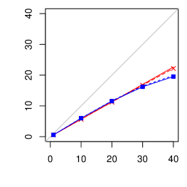
(a) default	(b) interleaved

Figure 4: Factored speedup curves for Maximal Independent Set benchmark. The straight, black curve represents the maximal speedup curve, the dotted, crossed one the idle-time specific curve, the dotted, blue one the inflation-specific curve, and the solid, blue one the actual speeedup curve.

4 Sources of Work Inflation

In this section, we present what we believe to be two particularly striking and subtle causes of work inflation. To simplify their presentation, we distill the causes of the work inflation in simplified benchmarks. Our measurements show that work inflation can affect speedups by nearly a factor two. In particular, we show that the speedups achieved may greatly vary with the size of the input data considered, and that they may greatly vary with the degree of optimizations that applies to pieces of code involved both in the baseline program and in the parallel program. In such circumstances, a higher degree of optimizations (which leads to reduced absolute execution time) may lead to smaller speedup values.

The benchmark.

To illustrate work inflation, we use a simple array microbenchmark, which is controlled by three parameters: array size $M$, a computation load $L$, a gap size $G$, and a number of repetition $R$. Given a set of values, the benchmark starts by allocating $M$ cells each of which contain a single 64-bit integer. The program then processes every cell of the array once, and repeats this entire process $R$ times. To process a cell $c$, the benchmark performs $L$ integer additions using the value at $c$ and writes the resulting value back into $c$. We implement the parallel for-loop by dividing the total range until a sufficiently small range of 1000 items, which are then processed sequentially.

When the gap size $G$ is equal to $1$, each thread processes a group of 1000 consecutive array items sequentially. When the gap size $G$ is more than $1$, threads still process groups of 1000 items, but acting over items spaced out by $G$ cells, in such a way that, ultimately, each array cell gets processed exactly once. To be precise, the $i$-th cell processed is that at index “$(iG+\lfloor\frac{iG}{M}\rfloor)\textsf{mod}M$” in the array. By considering values of $G$ greater than $1$, for example $32$, we are able to greatly increase the number of cache misses.

Input size and work inflation.

Our first experiments illustrate an interesting relationship between input data size speedups. On the one hand, it is well-known that, with small inputs, parallel programs may not generate sufficient parallelism to result in good speedups. On the other hand, large inputs that do not fit in the L3 cache lead to numerous cache misses, and they are typically associated with important levels of work inflation because the main memory becomes the bottleneck. As we show, however, there can be a range of input instances large enough to generate abundant parallelism, and nevertheless small enough to avoid significant work inflation. With such input instances, one is able to measure speedup values much greater than speedups that could be achieved when scaling to a larger number of cores or to larger input instances.

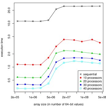
Figure 5: Runtime (top) and speedup (bottom) versus array size illustrated.

Figure 5 illustrates the runtime and speedup for our microbenchmark with different array sizes $M$ and different numbers of processors. In these experiments, we set the gap size to be $G=32$, and set the repeat count $R$ to be $\frac{4\cdot 10^{8}}{M}$ so that the total number of operations (a measure of the complexity of the benchmark) remains the same for all input sizes (i.e., $4\cdot 10^{8}$). The runtime curve (Figure 5, top) shows that compared with small input sizes, a sequential run, the topmost curve, is 2.2 times slower for inputs larger than $16\cdot 10^{6}$ —increasing from 11.3 seconds to 24.9 seconds. This outcome is expected, because the 30MB L3 cache of this processor approximately $4\cdot 10^{6}$ (64-bit) integers. What is interesting is that the slowdown is amplified in parallel runs. For example with $30$ cores, larger arrays are $3.7$ times slower compared with the smaller —increasing from 0.37 seconds to up to 1.37 seconds. While it is generally known that higher number of cache misses slow down a program execution, what is interesting here is that this slow down affects performance differently at different sizes. This behavior is likely due to the saturation of the memory bus at high parallel loads.

The fact that, when increasing the array size, parallel runs are slowed down more than sequential runs indicates that the work inflation increases with the array size. A direct consequence is that, as shown by the curve at the bottom in Figure 5, speedups can decrease significantly when operating on larger arrays. For example, with 40 cores, the speedup for small array is close to 35x, but with larger arrays it drops below 20x.

In summary, while with small inputs, the benchmark achives nearly perfect speedups, at large input sizes, the speedups decrease significantly. This suggests that work inflation can be significant and it should be accounted for by considering a range of input sizes, not just those input sizes that provide sufficient parallelism.

Work inflation and optimization.

Since speedups are calculated with respect to a baseline sequential program by calculating the ratio of the runtime of the sequential baseline to the runtime of the parallel code, it might be concluded that optimizing both programs to the same degree would suffice to perform a fair evaluation. In fact, the parallel code is often written by using the pieces of the sequential code, as this is often the easy and the natural thing to do. As we show next, speedups can be highly sensitive optimizations, not just because optimizations can improve the baseline performance—which is generally known and understood—but also because optimizations can impact serial and parallel code in different ways, by leading to different amounts of work inflation.

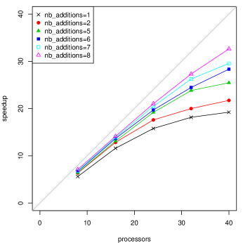
Figure 6: Impact of the computational load (number of additions performed between memory operations with gap size $1$.

To demonstrate the effect of optimization on work inflation, we consider our simple microbenchmark and run it with $M=600\cdot 10^{6}$ (that is, a 4.8Gb array), $R=1$, and different values of computational load $L$ ranging from $1$ to $8$. Recall that the microbenchmark performs $L$ additions after reading a cell and writes back the computed value to the memory. The differing values of $L$ suggest what can happen with highly optimized code $L=1$ and poorly optimized code $L=8$.

The plot Figure 6 shows the curves for different values of $L$ that we consider. The measurements show that the more the additions, the better the speedups. The implication is that additional work due to more additions creates relatively less work inflation. This implication is likely true because in parallel runs, all computation becomes memory bound, waiting for the memory operations to complete, during which time, cores can perform the addition operations (which commute) locally, without having the value of the cell being updated until it finally arrives. This property implies that the addition operations are parallelized by the hardware to overlap with the memory operations, reducing the relative significance of work inflation. We tested this hypothesis in two ways. First, we changed the addition operations to operations to commute with the reads; this change reduced the relative work inflation, ultimately improving the speedups. Second, we ran the benchmark with larger values of $L$, thereby increasing the memory latency for the sequential run, and thereby decreasing the relative work inflation.

In summary, when memory operations become a bottleneck in the parallel run, increased computational load due to non-agressive optimization can artifically increase speedup by reducing relative work inflation. It is therefore not sufficient to optimize the sequential baseline and the parallel code to the same degree. The baseline as well as the parallel code should be highly optimized in order to make sure that the effects of work inflation are not masked.

5 Related work

Prediction of parallel speedup.

Cilkview HeLeiserson10 , Intel Parallel Advisor IntelParallelAdvisor , Intel Parallel Amplifier IntelParallelAmplifier , and Kismet JeonGarciaLouie11 are software tools whose purpose is to profile and to analyze the potential scalability of programs on an arbitrary number of cores. Cilkview, Intel Parallel Advisor, and Intel Parallel Amplifier rely on user-supplied annotations, whereas Kismet tries to automatically detect parallelism in the application. Our method focuses instead on identifying the causes of suboptimal speedup of a given parallel program on a given machine with a fixed set of cores.

Modeling parallel performance.

Our techniques and those used for Cilkview share a common basis in the DAG model of computation. However, we use the DAG model in different ways to achieve different goals. On the one hand, the Cilkview profiler measures the work and span during the instrumented run of a parallel application on a single processor. The Cilkview analyzer predicts from the work and span the upper and lower bounds on the speedup curves that can be achieved by the application on an arbitrary number of processors. On the other hand, based on a mix of sequential and parallel runs, our analyzer plots, next to the actual speedup curve, a synthetic speedup curve that projects the amount of speedup lost due to idle time and parallelism overheads, allowing to visualize the amount of speedups lost due to memory effects.

In Cilkview, work and span are measured by number of instructions issued by the program, as opposed to wall-clock time. By considering instruction counts, the scalability prediction of Cilkview is completely oblivious to memory effects that could substantially harm scalability. Our work, although it is limited in that it considers only typical execution paths as opposed to worst-case execution paths, is able to deduce the amount of memory effects that impact the parallel runs.

Cilkview, being based on the work-span model, tries to evaluate the span. To that end, it considers a “burdened-dag model”, where the weight of fork nodes is burdened with an estimate of the cost of thread migration. The span measured in this burdened DAG gives a worst-case estimation of the span. In our work, we do not try to measure the span at all. Instead, we rely on the measure of the actual idle time, as explained in §2.6. Cilkview may nevertheless provide a complementary role in helping to estimate worst-case bounds on the idle time.

Identifying sequential bottlenecks in big programs.

The HPCToolkit TallentMellorCrummey07 ; TallentMellorCrummey09 is a software tool for profiling big parallel software that consists of many functions. HPCToolkit reports, on a per-function basis, estimated values of parallel idle time and parallelism overheads. Kremlin GarciaJeonDonghwan11 is another software tool whose purpose is to help guide the parallelization of large preexisting sequential programs. Kremlin, like HPCToolkit, focuses on the question: what parts of the program are most profitable to parallelize? As such, the primary focus of these tools is to assign blame to pieces of code that are imposing bottlenecks to parallelization.

In contrast, our focus is to analyze the performance of algorithms individually rather than to try to analyze the relative performance of multiple algorithms in the same program. Put another way, our focus concerns the stage after the programmer has identified a bottleneck code. At this point, the goal is to isolate the code and benchmark it independently to try and improve its scalability.

Often, blame-assigning tools, such as HPCToolkit and Kremlin, neglect to report in a synthetic way complementary pieces of information that would be helpful for understanding causes of poor speedup. Our factored speedup plots show a global view of the actual parallel performance of the optimized, production-ready code. In addition to providing a synthetic view of the data, our factored speedup plots show the speedup trends as the number of processors vary. The trends are useful, among other things, for extrapolating the ability of an algorithm to scale up to larger number of cores.

Profiling techniques.

The aforementioned profilers, as well as other related ones Reed93scalableperformance ; MohrAllenShendeWolf02 ; MooreWolfDongarraShendeAllenMohr05 , collect rich profiling data from instrumented runs of an application. Although sometimes useful, rich profiling data is not necessarily the best approach. Problematically, the instrumentation itself may affect the performance of the application being profiled. On the contrary, our approach relies on practically zero-overhead instrumentation and as such can be applied to production-ready user code.

In our approach, the required instrumentation consists of measurement of run time of the sequential baseline program, single-processor run time of the parallel program, run times of the parallel program on different subsets of the available processors, and total parallel idle time for each parallel run. All of these metrics are trivial to measure and can be readily measured in almost any platform. Many other profilers require substantial implementation effort in the form of compiler support or binary instrumentation.

To summarize, while we acknowledge the interest of full-program analysis and of rich instrumentation, we have found that our approach, despite being very lightweight, is able to report a large amount of useful information helping to analyse the scalability issues affecting a particular parallel algorithm.

6 Conclusion

On modern hardware, the impact of memory effects on the performance of parallel program is too important to be neglected. While these effects have shown difficult to model accurately, developers of parallel programs could greatly benefit of tools for analysing the relative impact of memory effects. In this paper, we have presented a simple model for the analysis of parallel computations. Our model is tailored for the analysis of experimental performance results, and it aims an analysing samples of executions. In that respect, it contrasts with the traditional work-span model, which provides a theory for computing bounds for worst-case executions.

Our model is based on the simple observation that, by sampling the execution time of single-processor runs and measuring idle time in parallel runs, we are able to deduce the amount of memory effects. Moreover, we have shown how to plot charts for visualizing the amount of speedups lost due to overheads, that lost due to idle time, and that lost due to memory effects. These charts allow to visualize not only the relative contribution of each source of slowdown, but also their trend as the number of processors grow. Although we have not seen such charts appear previously in the literature, they are, in our experience, helpful for the day-to-day development of parallel algorithms.

References

- [1] PREDATOR: Predictive False Sharing Detection, PPoPP ’14, New York, NY, USA, 2014. ACM.
- [2] Umut A. Acar, Arthur Charguéraud, and Mike Rainey. Scheduling parallel programs by work stealing with private deques. In Proceedings of the 19th ACM SIGPLAN Symposium on Principles and Practice of Parallel Programming, PPoPP ’13, 2013.
- [3] Guy E. Blelloch, Jeremy T. Fineman, Phillip B. Gibbons, and Julian Shun. Internally deterministic parallel algorithms can be fast. In Proceedings of the 17th ACM SIGPLAN symposium on Principles and Practice of Parallel Programming, PPoPP ’12, pages 181–192, 2012.
- [4] Richard P. Brent. The parallel evaluation of general arithmetic expressions. J. ACM, 21(2):201–206, 1974.
- [5] Philippe Charles, Christian Grothoff, Vijay Saraswat, Christopher Donawa, Allan Kielstra, Kemal Ebcioglu, Christoph von Praun, and Vivek Sarkar. X10: an object-oriented approach to non-uniform cluster computing. In Proceedings of the 20th annual ACM SIGPLAN conference on Object-oriented programming, systems, languages, and applications, OOPSLA ’05, pages 519–538. ACM, 2005.
- [6] Matteo Frigo, Charles E. Leiserson, and Keith H. Randall. The implementation of the Cilk-5 multithreaded language. In PLDI, pages 212–223, 1998.
- [7] Saturnino Garcia, Donghwan Jeon, Christopher M. Louie, and Michael Bedford Taylor. Kremlin: rethinking and rebooting gprof for the multicore age. In Proceedings of the 32nd ACM SIGPLAN conference on Programming language design and implementation, PLDI ’11, pages 458–469, New York, NY, USA, 2011. ACM.
- [8] Yuxiong He, Charles E. Leiserson, and William M. Leiserson. The cilkview scalability analyzer. In Proceedings of the 22nd ACM symposium on Parallelism in algorithms and architectures, SPAA ’10, pages 145–156, New York, NY, USA, 2010. ACM.
- [9] Intel. Cilk Plus. http://www.cilkplus.org/.
- [10] Intel. Intel Parallel Advisor 2011. http://software.intel.com/en-us/articles/intel-parallel-advisor/.
- [11] Intel. Intel Parallel Amplifier. http://software.intel.com/en-us/intel-vtune-amplifier-xe.
- [12] Intel. Intel threading building blocks, 2011. https://www.threadingbuildingblocks.org/.
- [13] Donghwan Jeon, Saturnino Garcia, Chris Louie, and Michael Bedford Taylor. Kismet: parallel speedup estimates for serial programs. SIGPLAN Not., 46(10):519–536, October 2011.
- [14] Bernd Mohr, Allen D. Malony, Sameer Shende, and Felix Wolf. Design and prototype of a performance tool interface for openmp. J. Supercomput., 23(1):105–128, August 2002.
- [15] Shirley Moore, Felix Wolf, Jack Dongarra, Sameer Shende, Allen Malony, and Bernd Mohr. A scalable approach to mpi application performance analysis. In Beniamino Martino, Dieter Kranzlmüller, and Jack Dongarra, editors, Recent Advances in Parallel Virtual Machine and Message Passing Interface, volume 3666 of Lecture Notes in Computer Science, pages 309–316. Springer Berlin Heidelberg, 2005.
- [16] OpenMP Architecture Review Board. OpenMP application program interface.
- [17] Daniel A. Reed, Ruth A. Aydt, Roger J. Noe, Phillip C. Roth, Keith A. Shields, Bradley W. Schwartz, and Luis F. Tavera. Scalable performance analysis: The pablo performance analysis environment. In In Proceedings of the Scalable parallel libraries conference, pages 104–113. IEEE Computer Society, 1993.
- [18] Nathan R. Tallent and John M. Mellor-Crummey. Effective performance measurement and analysis of multithreaded applications. In Proceedings of the 14th ACM SIGPLAN symposium on Principles and practice of parallel programming, PPoPP ’09, pages 229–240, New York, NY, USA, 2009. ACM.
- [19] Nathan R. Tallent, John M. Mellor-Crummey, and Michael W. Fagan. Binary analysis for measurement and attribution of program performance. In Proceedings of the 2009 ACM SIGPLAN conference on Programming language design and implementation, PLDI ’09, pages 441–452, New York, NY, USA, 2009. ACM.