Manifold Learning Using Kernel Density Estimation and Local Principal Components Analysis
Abstract
We consider the problem of recovering a dimensional manifold when provided with noiseless samples from . There are many algorithms (e.g., Isomap) that are used in practice to fit manifolds and thus reduce the dimensionality of a given data set. Ideally, the estimate of should be an actual manifold of a certain smoothness; furthermore, should be arbitrarily close to in Hausdorff distance given a large enough sample. Generally speaking, existing manifold learning algorithms do not meet these criteria. Fefferman, Mitter, and Narayanan (2016) have developed an algorithm whose output is provably a manifold. The key idea is to define an approximate squared-distance function (asdf) to . Then, is given by the set of points where the gradient of the asdf is orthogonal to the subspace spanned by the largest eigenvectors of the Hessian of the asdf. As long as the asdf meets certain regularity conditions, is a manifold that is arbitrarily close in Hausdorff distance to . In this paper, we define two asdfs that can be calculated from the data and show that they meet the required regularity conditions. The first asdf is based on kernel density estimation, and the second is based on estimation of tangent spaces using local principal components analysis.
Keywords: manifold learning, KDE, local PCA, ridges
1 Introduction
It is often the case that high-dimensional data sets have lower-dimensional structure taking the form of a manifold. Manifold learning consists of algorithms that take a high-dimensional data set as input and output a fit of the manifold structure. Many of these algorithms (such as Isomap, Laplacian eigenmaps, locally linear embedding, etc.) are used in practice and have a theoretical literature supporting them. Ma and Fu (2011) give a concise overview of these methods.
A drawback of most manifold learning algorithms is that if we are given data from a manifold, their output is not an actual manifold that is close to the original manifold. Fefferman, Mitter, and Narayanan (2016) develop an algorithm whose output is provably a manifold of certain smoothness. They start by defining an approximate squared-distance function (asdf) from the data in a manner that uses exhaustive search, utilizing the data only indirectly. Thus, a very large number of potential asdfs are examined before an approximately optimal one is chosen. In this paper, we do away with the exhaustive search, albeit in the specific case of noiseless data that is sampled uniformly from a manifold. Fefferman et al. (2016) prove a key theorem that states that as long as we are able to define an asdf meeting certain general conditions, their algorithm outputs a set that is a manifold with bounded smoothness and Hausdorff distance to the original manifold. We demonstrate two different methods of estimating the true manifold via asdfs that can be calculated from the data. The two asdfs in our paper are based on 1) kernel density estimation, and 2) approximating the manifold using tangent planes which are in turn approximated with local principal components analysis (PCA).
Ozertem and Erdogmus (2011) learn manifolds by forming a kernel density estimator (KDE) from the data points and finding its -dimensional ridges. We give a more precise definition later, but a ridge is essentially a higher-dimensional analog of the mode and is related to the output set from the algorithm of Fefferman et al. (2016). Ozertem and Erdogmus (2011) give a practical method for finding the ridges through a variant of gradient descent where the descent is constrained to the subspace spanned by the largest eigenvectors of the Hessian of the KDE. We state their algorithm in Section 5 of our paper and use it to produce simulation results. Although they only apply subspace-constrained gradient descent to find ridges of the KDE, the method is more general and can be used to find ridges of both of our asdfs.
1.1 Related work
Manifold learning has existed as an area of statistics and machine learning since the early 2000s. Some classical manifold learning algorithms are Isomap (Tenenbaum, De Silva, and Langford, 2000), locally linear embedding (Roweis and Saul, 2000), and Laplacian eigenmaps (Belkin and Niyogi, 2003). Many of these early algorithms rely on spectral graph theory and start off by constructing a graph which is then used to produce a lower-dimensional embedding of the data set. The theoretical guarantees are centered around proving that asymptotically, certain values such as the geodesic distance can be approximated to arbitrary precision.
More recently, there have been quite a few papers combining ridge estimation with manifold learning (including the work of Ozertem and Erdogmus, 2011). Some early results on ridge estimation are due to Eberly (1996), Hall, Qian, and Titterington (1992), and Cheng, Hall, Hartigan, et al. (2004). Ridge sets can be constructed to estimate a probability density or an embedded submanifold. Theoretical guarantees in this setting have been given by Genovese, Perone-Pacifico, Verdinelli, Wasserman, et al. (2012b), Genovese, Perone-Pacifico, Verdinelli, and Wasserman (2012a), Genovese, Perone-Pacifico, Verdinelli, Wasserman, et al. (2014), and Chen, Genovese, Wasserman, et al. (2015). Of these, the most relevant results for us are from Genovese et al. (2014). They prove that as the sample size goes to infinity, their ridge set gets arbitrarily close to an underlying manifold in Hausdorff distance. Fefferman et al. (2016) also define a procedure related to ridge estimation methods that can be used to estimate an underlying manifold. For our purposes, the major advances of their work are twofold. First, their method is general; as long as a function meets a few conditions, it can be used to define an estimator that can be made arbitrarily close to an underlying manifold in Hausdorff distance. Furthermore, they show that this estimator is itself a manifold with bounded reach (which measures how rough a submanifold can be). Second, their proofs rely on using the implicit function theorem concretely, allowing them to make quantitative statements about the bounds of interest.
1.2 Outline
Section 2 contains the technical background required to read our main results and proofs. This section starts off with background material on submanifolds, including key definitions, conventions regarding coordinates and projection operators, and important geometric results. Section 2.2 contains the model assumptions. Section 2.3 summarizes the major theorems we use from Fefferman et al. (2016). In Section 2.4, we summarize the algorithm from Ozertem and Erdogmus (2011) that we use to actually compute the putative manifold. Section 2.5 lists a few key concepts from empirical process theory. We include these because a few of our proofs are simpler when we work in the continuous setting and then argue that a similar result holds for a finite sample from the manifold. Sections 3 and 4 contain the main results of our paper. We provide the precise definition of the asdfs and prove that they do indeed meet the conditions required to apply the theorems contained in Section 2.3. Finally, we end with simulation results in Section 5 and a brief discussion in Section 6.
2 Technical background and assumptions
We now provide the definitions and major theorems that we rely on in the rest of the paper. The results we use the most often are Theorems 1, 2, 5, and 6; the rest of this section can be referred to as necessary.
2.1 Manifolds
This subsection is adapted from Fefferman et al. (2016). In the current paper, we use the terms manifold and submanifold interchangeably with compact imbedded -manifold. A closed subset is a compact imbedded -manifold if the following conditions hold. First, is compact. Next, there exists such that for every there exists a dimensional subspace of such that for a patch over of radius , centered at and tangent to at . A patch of radius over is a subset of where is a -function that is zero at the origin.
The tangent space can be defined in the usual way (corresponding to ) or by using the following definition which applies to arbitrary closed sets . At a point , is the set of vectors such that for all , there exists such that and . Let the tangent space be the set of all such that .
The geometric quantities of a submanifold that we are most concerned with are the -dimensional volume and the reach . The reach is the largest number such that all points within of have a unique closest point on . Intuitively, the reach governs how “rough” an embedded submanifold is. For example, the reach of a line with a sharp cusp is zero, and the reach of a linear subspace is infinite.
The following theorem due to Federer (1959) is useful for bounding the distance from a point on a manifold to the tangent space at a nearby point.
Theorem 1 (Federer’s reach condition).
Let be an embedded submanifold of . Then
In this paper, we assume regularity conditions on the manifold we draw samples from. We assume it is in , where is the family of boundaryless -submanifolds of the unit ball of with dimension , volume less than or equal to , and reach at least .
Let the tubular neighborhood be the set of all points within a distance of of . Now, for points and , denote the projection onto the tangent plane at by
A number of our proofs rely on defining the following sets:
is a cylinder centered at , and and are nearby regions of the manifold and tangent space, respectively. can also be defined as the projection of the cylinder onto the tangent space; i.e., as . These sets are especially useful because, as long as , they allow us to work with a local parametrization of the manifold. As mentioned earlier, manifolds can be defined locally as functions from the tangent space to the normal space. The functions we are working with are in the class ; i.e., they are once continuously differentiable and have a Lipschitz gradient. This is summarized in the next theorem.
Theorem 2.
Let . Let and . When is sufficiently small, there exists a function
such that
Additionally, there exists a constant such that .
The next theorem is from Krantz and Parks (2012). It states that has positive reach as long as it is embedded in a Euclidean space with strictly higher dimension.
Theorem 3.
Let be a -dimensional submanifold of . If , then has positive reach.
Now, suppose we want a discrete approximation of a manifold at a certain resolution. Let be an -net for if for every there is a such that . The following theorem states that the size of an net depends on the geometry of .
Theorem 4.
Let , and let be equipped with the Euclidean metric from . For any , there exists an net of consisting of at most points, where is a universal constant.
How well a manifold approximates a point set can be quantified through the empirical loss, which is defined as
where is the length of the projection from onto .
Given two subsets and of Euclidean space, we can measure the distance between them using the Hausdorff distance . This is defined as
It can be shown that, given adequate sampling density, two manifolds that are close in empirical risk to a given point set are also close in Hausdorff distance.
2.2 Model
We assume that we are provided with noiselessly sampled from the uniform distribution on . We take this approach to simplify calculations. The analysis would be similar if the sample came from a (potentially Lipschitz) density bounded away from zero.
2.3 Approximate squared-distance functions
For our purposes the most important results from Fefferman et al. (2016) are Theorem 13 and Lemma 14. We reproduce them below as Theorems 5 and 6, and give an adapted proof of the latter. It is beyond the scope of this paper to discuss the proof of Theorem 5. We merely note that it relies on the implicit function theorem, so there are concrete bounds on the constants and that control the geometry of the putative manifold.
Theorem 5 states that an approximate squared-distance function can be used to recover a manifold with arbitrary precision (with increasing sample size) as long as , a scaled version of the asdf, meets three conditions related to smoothness and curvature. The notation means that given a set of vectors , the partial derivative is computed successively in the directions . The third condition is the reason for the term asdf: for a small constant , is bounded both above and below by a multiple of , the approximate squared distance to the manifold.
Note that the function always has as its domain the unit ball (or a ball whose radius is not dependent on sample size). is not the asdf itself, but a related function applied locally after the coordinate system has been scaled up by a constant. This constant is usually a kind of bandwidth parameter that we decrease in order to get a more precise estimate of the manifold. For example, in Section 3, we have a scheme to decrease the bandwidth of the kernel density estimator, and is the KDE applied to coordinates scaled up by .
The output set from Theorem 5 is locally a smooth graph that lies within a tubular neighborhood of the manifold. Theorem 6 uses bounds on the smoothness of to show that it lies away from the boundary of the tubular neighborhood, and so it is itself a manifold. We show that it is in fact very close to the original manifold, giving a bound on the Hausdorff distance in terms of a constant that can be made as small as desired.
Theorem 5.
Suppose the following conditions hold for a function :
-
1.
is -smooth.
-
2.
, where and .
-
3.
For , and
for , where is an arbitrarily small constant depending only on and .
Then there are constants and depending only on and such that:
-
1.
For , let be the subspace of spanned by the top eigenvectors of . Let be the orthogonal projection from to . Then for and .
-
2.
There is a map
such that and for . The set of all such that
is a -smooth graph.
Theorem 6.
Let , and be the constants appearing in Theorem 5. Assume that is sufficiently small compared to . Define the putative submanifold
Then, is a submanifold of which has a reach greater than , where depends only on and . Furthermore, the Hausdorff distance is bounded above by .
The statement of this theorem assumes that we are provided with the output set from Theorem 5; that is, we are working in the scaled-up coordinates. In the original coordinate system, is contained in , where is the bandwidth. In this case, the reach is bounded below by , and is bounded above by .
Proof.
is locally the graph of a -smooth function . To prove that it is a manifold, it is sufficient to show that it does not intersect the boundary of the tubular neighborhood . Since Theorem 5 gives bounds on , we can show by contradiction of the mean value theorem that every point on is within of .
Suppose there exists a point on which is at a distance greater than from . Let . By Theorem 5, there is a point such that . Let be the vector . Let define a curve on whose endpoints are and . The existence and smoothness of are guaranteed by , the -smooth function that locally defines . The mean value theorem states that there exists a point such that
Since is sufficiently small compared to , can be made as large as desired. This contradicts the bound and shows that lies away from the boundary of . In fact, the expression in the third line above must be less than , which shows that . Theorem 5 states that every point on is within of , so we have the desired bound on the Hausdorff distance.
By Theorem 1, the reach of is defined as follows:
Let be a constant depending on and . If , then
Now, suppose . If and are close together, this quantity is controlled by the second derivative of the function locally defining . That is, is on the order of , implying that
for some constant . Therefore,
∎
2.4 Ridges and gradient descent
To actually find a putative manifold using an approximate squared-distance function , we can use a method introduced by Ozertem and Erdogmus (2011). Let and be the gradient and Hessian of , respectively. At a point , let be the eigenvectors of associated with the eigenvalues (listed in decreasing order). Let be the subspace of spanned by the top eigenvectors of . Recall that is the orthogonal projection from to . Note that , where is a matrix whose columns are .
Ozertem and Erdogmus (2011) give an algorithm to compute the set
which is termed the -dimensional ridge of . This is, of course, the local definition of from Theorems 5 and 6. In order to find a ridge, an initial set of points is chosen and then iteratively shifted in the direction until a tolerance condition is met. This is essentially a subspace-constrained variant of gradient descent.
2.5 Empirical processes
In Section 3, we need to bound various quantities that are functions of the kernel density estimator. This is difficult to do because they are empirical averages over a finite number of samples. It is easier to bound the expectation of these quantities and then bound their difference using results from empirical processes, which we summarize here.
Let be a class of functions from . If consists of bounded functions, the empirical Rademacher average is given by
where is an i.i.d. sample from the distribution and is a vector of Rademacher random variables. (Rademacher random variables take the values with equal probability). Letting denote the empirical distribution on , the following holds for :
It is usually difficult to calculate directly from the definition. However, the next theorem states an upper bound that is dependent on the size of , which is often easy to estimate. Let the covering number be the minimum number of elements in an -net of with respect to the norm . Let the metric entropy be defined as . The Rademacher complexity can be bounded using a modified form of Dudley’s entropy integral (Sridharan and Srebro, 2010):
Theorem 7 (Modified Dudley’s integral).
3 Kernel density estimation
Consider the kernel density estimator
where and (the tubular neighborhood of with width ). The denominator of has raised to the power and not because we are trying to estimate a -dimensional surface. In Theorem 16, we show that a function based on can recover a manifold when we are given noiseless samples from .
3.1 Definition of the asdf
Recall that Theorem 5 must actually be applied in a coordinate system scaled by a bandwidth parameter that becomes more precise with increasing sample size. For the kernel density estimator, this parameter is, of course, . (If we do not scale by , it is clear that is bounded above by an increasing function of instead of a universal constant ). To this purpose, make the following transformations:
Note that the geometric properties of change in the obvious ways: the reach becomes and the volume is . In the transformed case, let , , and denote the analogs of the obvious quantities. For the projection of onto , let and . Recall that these are regions of and , respectively, which are near the point . Define the normalizing factor
The appropriate estimator to analyze is any convenient function of , where
We choose to work with as our potential asdf. The first condition from Theorem 5 follows immediately, as seen in the following lemma.
Lemma 8.
is -smooth.
Proof.
is -smooth, so by linearity, is -smooth. By the chain rule, is -smooth. ∎
3.2 Selecting the bandwidth
The procedure we assume is that a fixed value of is chosen by the experimenter as well as a value of that depends on . Without making any claims about optimality, we choose . We prove that there exists a lower bound for given . We then use empirical processes to show that concentrates around , and is within of with high probability. Since is a decreasing function of the sample size , we can increase until giving us a lower bound for . This allows us to derive an upper bound for . We also find an expression for in terms of and use this to show that condition 3 of Theorem 5 holds. If is not small enough, we can repeat this procedure using a fixed value of in each subsequent iteration.
3.3 Bounding in expectation
To prove the second and third conditions, we need upper and lower bounds for . It is more convenient to work initially in the continuous setting, which amounts to bounding . This is the Gaussian kernel integrated against , the measure that is uniform with respect to the volume form. Explicitly,
Points on that are far away from do not contribute very much to the value of this integral. In fact, the value of is very close to
where is the projection of onto . Define its approximation
where is the -dimensional Lebesgue measure on .
Decreasing corresponds to estimating with greater precision. Even though this expands the unit ball, leading to , the ratio . This implies that and are shrinking relatively closer and closer to , and is very close to an affine space. Thus, we expect and to grow closer together. To prove this, we first need to show that the pushforward of the uniform measure on the manifold has a density that is close to the uniform density on . Of course, we don’t want this to be a proper density on ; we want it to have the same total measure as . In the following lemma, we quantify how much can deviate from on .
Lemma 9.
Let , and let . The pushforward of to has density on with respect to such that
Proof.
Assume that is the origin and the first coordinates lie in . is a submanifold of defined locally by the function that maps . Recall from Theorem 2 that is a function whose Jacobian has a Lipschitz constant bounded above by . evaluated at is 0 since is tangent to at ; this implies within a radius of , where is the Frobenius norm. We can find the desired bound on by finding the ratio of the volume elements of and , normalizing this so it integrates to one over , and multiplying by . has Jacobian , allowing us to write
Let be the eigenvalues of . is positive semidefinite, so . Then,
Since the map from to is a contraction, . Clearly, we also have
which is enough to show the lemma. ∎
We can use this bound on to simplify the integration of functions over . As we mentioned earlier, is a function of an integral whose major contribution comes from the region . (A crude bound suffices for the contribution from the region ). In the following lemma, we show that and are very close together. By using the pushforward we can perform both integrals over using Lebesgue measure. To do so we need a bound on the ratio of to (which we have) as well as a bound on the ratio between the integrands. We find that and are within a constant of each other. By decreasing , can be made as small as desired.
Lemma 10.
Let , and let be the projection of onto . Then, , where
Proof.
Assume that is the origin and is identified with the first coordinates. The following chain of inequalities holds, where , is a point on the manifold, and is the Jacobian of :
The first term in the last line comes from Lemma 9. A Taylor expansion (valid for ) shows that
Therefore,
as long as is smaller than a controlled constant. To bound the other term, we use the law of cosines in conjunction with Theorem 1, which shows that
Let be the angle between and . Then, we have:
Thus, , where is defined in the statement of the lemma. ∎
To actually find the lower bound for , we bound in the next lemma by using a -dimensional Gaussian concentration inequality. The upper bound is much simpler to derive; we include it as well. These bounds are important in verifying the second and third conditions of Theorem 5. The third condition essentially says that our function is an approximate squared-distance function. That is, given a point and its projection , we should have upper and lower bounds that are close to . Since our putative asdf is , we need bounds for that are within a multiplicative factor of . In the proof of the following lemma we find these pointwise bounds.
The second condition requires that we find an upper bound for . This derivative consists of terms that have powers of in the denominator and combinations of powers of partial derivatives of in the numerator. Thus, we need a uniform lower bound for over ; this follows by taking the infimum of the pointwise bound over the tubular neighborhood. We also need bounds for , but we defer these to the proof of Lemma 13.
Lemma 11.
is bounded in expectation. More precisely, , where
furthermore, , where
Proof.
Let be the projection of onto , and let .
where the second inequality is due to Lemma 10. By orthogonality, , so we rewrite the integral over as follows:
where the probability is with respect to a dimensional multivariate Gaussian with covariance . Letting be the origin for simplicity, we know from standard Gaussian concentration results (Boucheron, Lugosi, and Massart, 2013) that
for . We can calculate and then get a bound for by using Jensen’s inequality.
Make the substitutions
and let
We have
The product in the third line telescopes to ; simplifying yields the fourth line.
It follows that . Setting (and assuming that is small enough so ), we see that
Consequently,
The first part of the lemma follows by taking the infimum over .
To find an upper bound, first write the expectation as
The first term can be bounded as follows:
Now consider . Since and , we have . This gives us the following bound for the second term as long as is large enough:
Thus, for ,
∎
Note that the values we chose for and are appropriate given our calculations in this section. For decreasing , we would like for to grow closer to in Lemma 9 and for to tend to zero in Lemma 10; we also need , the Gaussian concentration probability, to grow closer to 1 in the previous lemma. Our choice of is appropriate given these constraints. For small enough, and . Thus, and .
3.4 Finite sample bounds for and
In Lemma 11, we proved a statement about whereas we really need a statement about . We can use methods from empirical processes to relate these quantities. Let consist of functions where each has the form with . Here, is fixed, and each corresponds to a different . Note that is equivalent to and is equivalent to . We have the tools to prove that for ,
where is a function of and . We rewrite the form of the probability bound in part (a) of Lemma 12 so that it is in terms of and .
In part (b) of Lemma 12, we prove a similar concentration bound for particular derivatives of . Let consist of functions where each is of the form with , , and . These functions are involved in finding an upper bound for .
Lemma 12.
Let be the class of functions consisting of indexed by . For a given and , let be the class of functions consisting of indexed by .
-
(a)
For ,
where
and
-
(b)
For ,
where
and
Proof.
We can bound through a method from empirical processes by first determining the covering number of and then using Dudley’s integral. Since is a class of Lipschitz functions parametrized by points in , we can relate its covering number to the covering number of this parameter space.
From empirical process theory, we know that
is the Rademacher complexity of , which can be bounded using Theorem 7. Let be the covering number at scale with respect to norm . Then,
The second inequality is well-known. Each is parametrized by and is at most -Lipschitz in this parameter. If we can calculate , we can also bound the covering number of by relating it to the covering number of the tubular neighborhood.
That is,
where the second line follows from taking a 1/100-net of , placing unit -balls at each net point, and then finding an -net of those.
Now we find . For simplicity, assume has coordinates that have been centered around any point on the manifold. By the symmetry of , we only need to consider one coordinate.
Since ranges between 0 and 1, . Define ; then,
Using the monotonicity of and the square root,
Thus, with high probability,
which proves (a).
The proof of part (b) is nearly the same, with the only difference being in the covering number of the parameter space. If each is at most -Lipschitz, then
where . Since
we have
In the third line, are the components of . The final line follows by the Cauchy-Schwarz inequality, which shows that and . Differentiating with respect to and setting equal to zero shows that the supremum is achieved at . We can substitute this back in to set
∎
It follows directly that with high probability. For large enough , . In the next lemma, we prove that a corresponding result holds for (which is exactly the second condition from Theorem 5). The derivation is more technical but the intuition is based on the arguments in Section 3.3.
Lemma 13.
for , , and depending only on and .
Proof.
Start by defining
where is the projection of onto . Then,
A result due to Nemirovski (2004) shows that
for -smooth , implying that we do not need to bound mixed partials.
It is straightforward to calculate . (The supremum is also over ). To get an upper bound for , we first write it as an expression involving powers of and partials of . For example, if ,
Faa di Bruno’s formula is an explicit representation of this expression; the number of terms and the coefficients depend on . We can find a suitable if we can calculate a lower bound for and an upper bound for where . The first bound follows from two previous lemmas. Lemma 11 shows that , and Lemma 12 shows that is within of its expectation with high probability. Since and can be made smaller than , with high probability for sufficiently large. is a function of , and is a function of .
To bound the partials of , we start off by using the second part of Lemma 12, which shows
Let be the origin and let the first coordinates lie in . We can write the expectation as
We first bound the integral over . For large enough, the local extrema of with respect to lie within . Since
is decreasing with increasing in . The following holds, where :
The integral over can be bounded by relating it to the corresponding integral over . Let be the projection of onto . Then,
The third line comes from relating and (Lemma 9) and bounding the change in the integrand due to projecting onto . We do not project because it can equal zero. The fourth line follows by noting that by orthogonality and that by Federer’s reach condition. The reach condition also shows that is a polynomial whose terms either lie in or have arbitrarily small coefficients. This can be used to bound the integral. Starting off by applying the triangle inequality for integrals and then the Cauchy-Schwarz inequality, we have
The second line holds because and can be bounded using the triangle inequality. The third line follows after expanding , substituting in the bound for , and rearranging. Each term in the summation can be made arbitrarily small, which gives the fourth line. This integral is a function of the moments (of order or less) of a -dimensional Gaussian with covariance . We can calculate it using spherical coordinates, following the calculation of in Lemma 11. We have
Therefore, for large enough ,
If is large enough, will be smaller than with high probability, implying that . Let be the value of for which this is maximized. Each term of is bounded above in absolute value by a multiple of raised to a power less than or equal to . Therefore, using the triangle inequality and letting , , a constant. The factors of in and cancel each other out, so is a function of and . Setting yields the lemma. ∎
3.5 is an asdf
In the next two lemmas, we prove that the third condition of Theorem 5 holds. Recall from the proof of Lemma 11 that can be bounded above and below to within a multiplicative factor of . By taking logarithms and defining a suitable constant , we show in Lemma 14 that the third condition holds for . In Lemma 15, we show that this condition also holds for as long as we modify to take into account the concentration bound from Lemma 12.
Lemma 14.
For and the projection of onto ,
for , with depending on .
Proof.
Let and let be its projection onto . Then we can bound by calculating the expectation separately over and :
The first term can be bounded as follows:
Now consider . Since and , we have . This gives us the following bound for the second term:
Thus, letting
we have
The second inequality holds because is arbitrarily small for small , so we can use the Taylor expansion
Next, we find a lower bound for as in Lemma 11.
Now, let and . We have shown the following:
Since , we can add to the left-hand side, to the middle, and to the right-hand side while preserving these inequalities. Let , , and . Then, we have
∎
Lemma 15.
With high probability, for and the projection of onto ,
for , with depending on .
Proof.
We have proven all the conditions necessary in order to show that is an asdf. We summarize this in the next theorem, which is the major result of this section. We also prove that the constants we have defined are small enough to apply Theorem 6 and state that is a manifold with desirable properties.
Theorem 16.
is an approximate squared-distance function that meets the conditions in Theorem 5. Consider the output set
in the original coordinate system (i.e., the coordinates not scaled by , where is the bandwidth of the KDE). By Theorem 6, is a manifold whose reach is bounded below by , where is a constant depending on and . converges to in Hausdorff distance for increasing ; more specifically, .
Proof.
Since is a constant, the first two conditions from Theorem 5 hold by Lemmas 8 and 13. The third condition holds by Lemma 15. Thus, is an asdf.
For to be a manifold, must be sufficiently small with respect to . We will show that for a small enough and large enough , (our choice of ) can be made as small as needed. Recall that and . This implies
which can be made as small as desired. and can be bounded by using the fact that if is sufficiently small. For a small enough ,
which gives the bound
Similarly,
As tends to zero, so do these quantities. Finally, for large enough , is sufficiently small such that is as small as necessary. For a small enough and a large enough , . This is sufficient to apply Theorem 6, which implies that is a manifold with bounded reach that converges to in Hausdorff distance. The Hausdorff distance is , which is . ∎
4 Local principal components analysis
A manifold can be approximated by a finite collection of tangent spaces centered at a sufficiently dense set of points sampled from . Fefferman et al. (2016) use this as motivation to define the concept of a cylinder packet; they also define a function and show that it is an asdf when coupled with a suitably constructed cylinder packet. In this section we show that we can estimate tangent spaces directly from the data to create a cylinder packet; this leads to the construction of an approximate squared-distance function that satisfies Theorems 5 and 6 and produces a putative manifold.
4.1 Definition of the asdf and selection of the bandwidth
Let be a collection of cylinders with centers . Each cylinder is isometric to . We choose so that it tends to zero but remains large compared to the distance between a sample point and its nearest neighbors. Since we are assuming uniform support on , for large we can choose on the order of for a small value of .
Let be a proper rotation of , a translation, and a composition of a proper rotation and translation that moves the origin to and rotates the -dimensional cross-section of to . Define
where , , is the squared distance from to the -dimensional cross-section of and is a bump function such that
-
1.
for
-
2.
for and or
-
3.
, a controlled constant for all
-
4.
for .
Note that whether or not satisfies Theorem 5 depends on our choice of ; for convenience, we refer to the pair as a putative asdf. measures the squared distances to the central cross-section of each cylinder containing a given point , and averages them using the bump function . Let be a related function defined by , where is an isometry that fixes the origin at and identifies the first coordinates with . is essentially analyzed in a coordinate system scaled up by . This is analogous to our analysis of the kernel density estimator in the previous section, where we scaled the coordinate system by .
4.2 Cylinder packets
In order for to be an asdf, needs to be a cylinder packet, which is a collection of cylinders that satisfies the geometric constraints given below in Definition 17. These conditions ensure that a cylinder packet doesn’t contain pairs of cylinders that overlap too much or intersect at too great of an angle. This is motivated by our desire to estimate a manifold with bounded reach.
Definition 17 (Cylinder packet).
Let be a collection of cylinders as above. is a cylinder packet if it satisfies the following conditions:
-
1.
The number of cylinders is less than or equal to a constant factor times .
-
2.
Consider the set of cylinders that intersect and perform the rigid-body motion . For each , there exists a translation and a proper rotation fixing so that
-
(a)
For , is a translation of by a vector with norm at least .
-
(b)
forms a net of the -dimensional cross-section of .
-
(c)
For and , .
-
(d)
For , .
-
(a)
In Lemmas 16 and 17 due to Fefferman et al. (2016), it is shown that satisfies Theorem 5 when is a cylinder packet, meaning that is an asdf. We include this towards the end of this section as Theorem 23 and provide a sketch of the proof.
In the next lemma we construct a collection of cylinders whose central cross sections are derived from the tangent planes of the manifold and show that it is indeed a cylinder packet. The putative manifold actually has reach , so the right-hand sides of conditions 2(c) and (d) in Definition 17 can be within a constant factor of what is given above.
Lemma 18.
First, construct a set of centers. Assume the sample size is large enough to contain a net of such that no two net points are within of each other. Let be the collection of cylinders with centers and central cross sections contained in . Then, is a cylinder packet; we call it an ideal cylinder packet.
Proof.
We show that the conditions in Definition 17 hold. Fix an and consider the set of cylinders that intersect . Perform the rigid-body motion so that we are working in a convenient coordinate system. For each , define as a rotation fixing and rotating the central cross section of so that it is parallel to . Also, define as the translation that subsequently moves the central cross section so that it lies in . Lemma 4 implies the first condition.
Let be the projection of onto . Federer’s reach condition implies that
Condition 2(d) holds since the right hand side must be less than . Since , we also have
where the last line follows by a Taylor expansion. Since this can be made arbitrarily close to , and Condition 2(a) is satisfied. Condition 2(b) follows from the fact that we started off with a net of the manifold; projecting onto contracts interpoint distances so we end up with a net of the tangent space.
To show the bound in 2(c), we need an expression for the angle between two nearby tangent spaces (in this case and ). In Lemma B.3 from a paper by Boissonnat, Dyer, and Ghosh (2013), it is shown that the sine of the largest principal angle between and is less than or equal to , which is in our setup. Now, translate the origin to and translate so that it contains . Without loss of generality, let . Let and be orthonormal bases for and , respectively, so that the angle between and is the principal angle . Define as the rotation that maps onto . Let be the components of and with respect to the appropriate bases. Then we have the following:
Using the law of cosines, . From the bound on and a Taylor expansion of , we can show
for large enough . Thus,
which shows 2(c). ∎
Corollary 19.
First, construct a set of centers. Assume the sample size is large enough to contain a net of such that no two net points are within of each other. The collection of cylinders with centers and central cross sections within of in operator norm is a cylinder packet; we call it an admissible cylinder packet.
4.3 Constructing an admissible cylinder packet with local PCA
Usually we only have access to points sampled from the manifold and not their associated tangent spaces. It is easy to see that we can also construct a cylinder packet if we can estimate the tangent spaces accurately enough (as stated in Corollary 19). Let be a collection of cylinders constructed by using the same net points as in Lemma 18 and performing local PCA to estimate the -dimensional cross-sections. In this section, we show that is an admissible cylinder packet. The -dimensional cross-sections are estimated as follows. Given a sample point , we construct the PCA matrix , where has columns consisting of the sample points lying within . (We are using a coordinate system centered at whose first coordinates lie in ). Using the eigenvectors of , we can get an estimate of the tangent space at . We show that this is close to the true tangent space by using the Davis-Kahan theorem. The version stated below is due to Yu, Wang, and Samworth (2015).
Let denote the Frobenius norm of a matrix. Suppose both have orthonormal columns. Theorem 20 gives an upper bound on , where is the diagonal matrix whose diagonal consists of the principal angles between the column spaces of and and is defined entrywise. The principal angles are given by , where are the singular values of .
Theorem 20 (Davis-Kahan Theorem).
Let be symmetric, with eigenvalues and respectively. Let and assume . Let and have orthonormal columns satisfying and for . Then
We also make use of the following concentration inequality due to Ahlswede and Winter (2002). Let mean that is positive semidefinite.
Theorem 21.
Let be i.i.d. random positive semidefinite matrices with expected value and . Then for all ,
We now prove the key result of this section.
Theorem 22.
Let be a point sampled from . Translate to the origin, and let the first coordinates lie in . Let be a matrix whose columns consist of the sample points lying within . Let be a matrix whose columns are the projections of onto . Construct the matrices and , and let and be their respective matrices of eigenvectors. Then, w.h.p.,
where .
Proof.
Clearly, increases with . We can assume the matrices in the statement of the theorem can be defined. We apply Theorem 20 with and corresponding to and , respectively.
We start off by bounding the numerator . This is easiest if we consider as a perturbation of by the matrix since we can control using Federer’s reach condition. This gives:
Therefore,
Because each column of X has norm less than or equal to , . By Federer’s reach condition, we have
which implies that . Thus,
Now we need to bound . Let be the eigenvalues of , and let be the eigenvalues of . We see that . So, we only need a lower bound for , which we can get by relating its value to through a concentration inequality. Assuming the first coordinates are aligned with the eigenvectors of , is the variance in the direction . is the population covariance matrix of the probability measure on that is the pushforward of the uniform measure on . From Lemma 9, we know has a density that is greater than or equal to multiplied by a normalizing factor, which in this case is just .
We have the following bound for :
The third line follows by a change of coordinates. Substitute
and let
The integral in the fourth line can be evaluated by noting that , , and for . We can simplify (by telescoping)
Therefore,
and are zero outside the upper left block. Call their nonzero blocks and , respectively; clearly these matrices have eigenvalues and . can be written as the empirical average , where the are the first coordinates of the . Note that . For large enough, this implies . Additionally, since is the smallest eigenvalue of , we have . This is sufficient to apply Theorem 21. So, for all ,
The matrix interval is in terms of the positive semidefinite ordering, so w.h.p. This implies .
4.4 is an asdf
In Theorem 23, we sketch a proof that is an asdf for an arbitrary cylinder packet ; we also show that Theorem 6 applies. Since we showed that is an admissible cylinder packet, it follows immediately that is an asdf.
Theorem 23.
Assume that we are given a cylinder packet . is an approximate squared-distance function that meets the conditions in Theorem 5. Furthermore, by Theorem 6, the output set (in the original coordinate system)
is a manifold whose reach is bounded below by , where is a constant depending on and . converges to in Hausdorff distance for increasing ; more specifically, .
Proof.
is -smooth by the chain rule and the smoothness of the projection, distance, and bump functions. for , , and depending only on and . This is true by the chain rule since the bounds on the derivatives of the bump function and the distance function can be directly calculated. After rescaling by , these depend only on and .
The third condition is satisfied by setting equal to , where is a constant depending on the geometry of . Let . If is a cylinder packet, the distance from to the central cross-section of any cylinder containing is on the order of . is a rescaled convex combination of the squared distance between and the central cross section of the cylinders containing it. That is, is essentially , where and the depend on . Thus, setting to satisfies the third condition of Theorem 5 for appropriate values of and :
where , with depending on .
For Theorem 6 to apply, must be sufficiently small with respect to . This is clearly true because , which can be made as small as desired. The Hausdorff distance is , which is . ∎
Theorem 24.
, where is a cylinder packet constructed using local PCA is an approximate squared-distance function that meets the conditions in Theorem 5. Furthermore, by Theorem 6, the output set
is a manifold whose reach is bounded below by , where is a constant depending on and . converges to in Hausdorff distance for increasing ; more specifically, .
5 Simulations
In this section, we present simulation results showing that the two asdfs considered in this paper can be used to find a discretized version of a putative manifold. All simulations were performed using the following gradient descent algorithm based on subspace-constrained mean shift (Ozertem and Erdogmus, 2011).
-
1.
Initialize a mesh of points on which to perform gradient descent. They can be sample points with or without added noise.
-
2.
Perform the following for each mesh point :
-
(a)
Calculate the gradient and the Hessian of the asdf .
-
(b)
Let be a matrix whose columns are the eigenvectors corresponding to the largest eigenvalues of .
-
(c)
Calculate and take a step in this direction.
-
(d)
Go to step (a) until a tolerance condition is met.
-
(a)
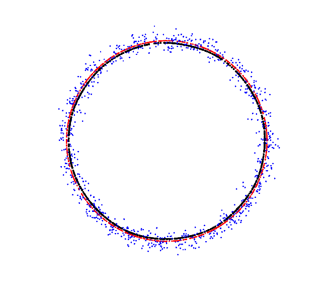
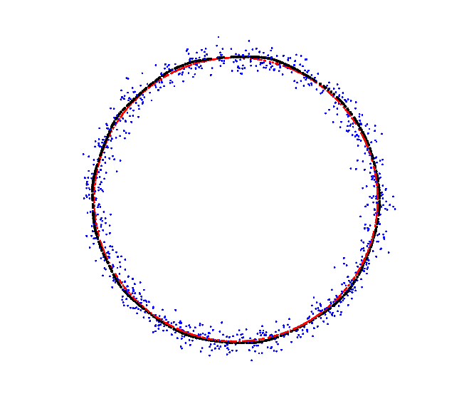
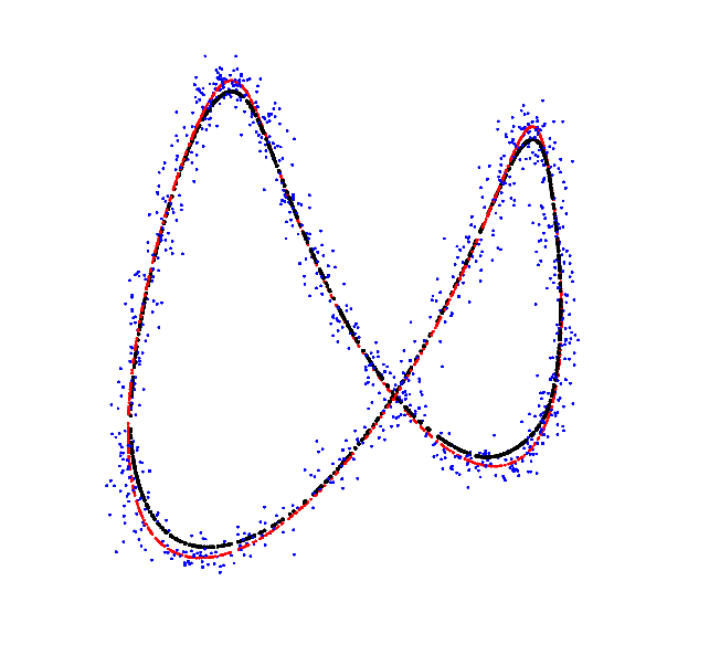
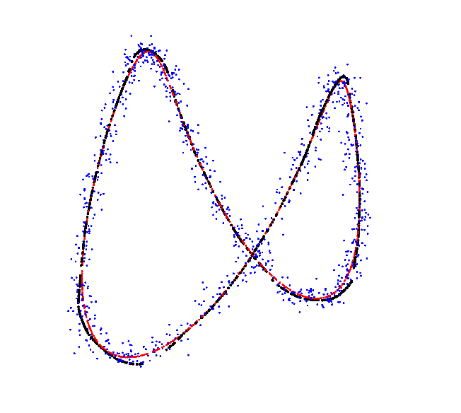
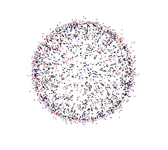
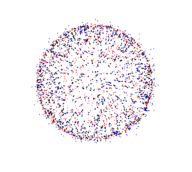
We applied this algorithm to data points sampled from three different manifolds contained in the unit ball of a Euclidean space: a circle embedded in , a closed curve embedded in , and a sphere embedded in . We sampled 1000 points from each manifold and used this data to construct asdfs based on KDE and local PCA. We then sampled 1000 additional points and added Gaussian noise with a standard deviation of 0.05; these were used as the starting mesh points. Finally, we ran the algorithm and took the final output to be points lying on the putative manifold. Figure 1 shows an example of each of the three manifolds for each asdf. To get a sense of the accuracy of this procedure, we found the RMS distance of each putative manifold to a 10000 point sample (i.e., an approximate net) derived from the original manifolds. The average RMS distance from 100 trials is given in Table 1.
| Circle | Curve | Sphere | |
|---|---|---|---|
| KDE | 0.000433 | 0.000990 | 0.00221 |
| Local PCA | 0.000146 | 0.000453 | 0.000603 |
6 Discussion
In this paper, we showed that if we are provided with data sampled from a manifold , we can use two different asdfs to construct an estimator of . The asdfs are based on kernel density estimation and local PCA, which are conceptually easy to understand and mainstays of nonparametric estimation. The estimator is a manifold itself, and there are concrete bounds on its geometry (for example, its reach). These bounds are derived from an application of the implicit function theorem and are given in a key theorem of Fefferman, Mitter, and Narayanan (2016). Our contribution in this paper is to create asdfs that can be calculated directly from the data as well as to give bounds on the reach and Hausdorff distance that depend on the sample size and properties of the asdfs. In the future, we aim to work on several natural extensions of our results. It remains to be seen what can be said about an estimator derived from a sample contaminated with noise (potentially bounded or sub-Gaussian). Additionally, it would be of theoretical interest to see how precise we can make the constants in this paper, including the ones derived from Fefferman et al. (2016).
Acknowledgments
We are grateful to Charlie Fefferman and Sanjoy Mitter for several illuminating discussions on local PCA. We would also like to thank Charlie for discussing the main results from Fefferman et al. (2016) with us, especially Theorem 13 and Lemma 14. We are also grateful to Marina Meila, Johannes Lederer, Emo Todorov, and Yen-Chi Chen. Their comments on a preliminary draft of this paper were very helpful. We would further like to thank Yen-Chi for advice that we used in constructing the simulation studies used in this paper. Finally, both authors were partially supported by NSF grant DMS 1620102.
References
- Ahlswede and Winter (2002) Rudolf Ahlswede and Andreas Winter. Strong converse for identification via quantum channels. IEEE Transactions on Information Theory, 48(3):569–579, 2002.
- Belkin and Niyogi (2003) Mikhail Belkin and Partha Niyogi. Laplacian eigenmaps for dimensionality reduction and data representation. Neural Computation, 15(6):1373–1396, 2003.
- Boissonnat et al. (2013) Jean-Daniel Boissonnat, Ramsay Dyer, and Arijit Ghosh. Constructing intrinsic Delaunay triangulations of submanifolds. arXiv preprint arXiv:1303.6493, 2013.
- Boucheron et al. (2013) Stéphane Boucheron, Gábor Lugosi, and Pascal Massart. Concentration Inequalities: A Nonasymptotic Theory of Independence. OUP Oxford, 2013.
- Chen et al. (2015) Yen-Chi Chen, Christopher R Genovese, Larry Wasserman, et al. Asymptotic theory for density ridges. The Annals of Statistics, 43(5):1896–1928, 2015.
- Cheng et al. (2004) Ming-Yen Cheng, Peter Hall, John A Hartigan, et al. Estimating gradient trees. In A Festschrift for Herman Rubin, pages 237–249. Institute of Mathematical Statistics, 2004.
- Eberly (1996) David Eberly. Ridges in Image and Data Analysis, volume 7. Springer Science & Business Media, 1996.
- Federer (1959) Herbert Federer. Curvature measures. Transactions of the American Mathematical Society, pages 418–491, 1959.
- Fefferman et al. (2016) Charles Fefferman, Sanjoy Mitter, and Hariharan Narayanan. Testing the manifold hypothesis. Journal of the American Mathematical Society, 2016.
- Genovese et al. (2012a) Christopher R Genovese, Marco Perone-Pacifico, Isabella Verdinelli, and Larry Wasserman. Minimax manifold estimation. The Journal of Machine Learning Research, 13(1):1263–1291, 2012a.
- Genovese et al. (2012b) Christopher R Genovese, Marco Perone-Pacifico, Isabella Verdinelli, Larry Wasserman, et al. Manifold estimation and singular deconvolution under Hausdorff loss. The Annals of Statistics, 40(2):941–963, 2012b.
- Genovese et al. (2014) Christopher R Genovese, Marco Perone-Pacifico, Isabella Verdinelli, Larry Wasserman, et al. Nonparametric ridge estimation. The Annals of Statistics, 42(4):1511–1545, 2014.
- Hall et al. (1992) Peter Hall, Wei Qian, and DM Titterington. Ridge finding from noisy data. Journal of Computational and Graphical Statistics, 1(3):197–211, 1992.
- Krantz and Parks (2012) Steven G Krantz and Harold R Parks. The Implicit Function Theorem: History, Theory, and Applications. Springer Science & Business Media, 2012.
- Ma and Fu (2011) Yunqian Ma and Yun Fu. Manifold Learning Theory and Applications. CRC press, 2011.
- Nemirovski (2004) Arkadi Nemirovski. Interior Point Polynomial Time Methods in Convex Programming. http://www2.isye.gatech.edu/~nemirovs/Lect_IPM.pdf, 2004.
- Ozertem and Erdogmus (2011) Umut Ozertem and Deniz Erdogmus. Locally defined principal curves and surfaces. The Journal of Machine Learning Research, 12:1249–1286, 2011.
- Roweis and Saul (2000) Sam T Roweis and Lawrence K Saul. Nonlinear dimensionality reduction by locally linear embedding. Science, 290(5500):2323–2326, 2000.
- Sridharan and Srebro (2010) Karthik Sridharan and Nathan Srebro. Note on refined Dudley integral covering number bound, 2010.
- Tenenbaum et al. (2000) Joshua B Tenenbaum, Vin De Silva, and John C Langford. A global geometric framework for nonlinear dimensionality reduction. Science, 290(5500):2319–2323, 2000.
- Yu et al. (2015) Yi Yu, Tengyao Wang, and Richard J Samworth. A useful variant of the Davis–Kahan theorem for statisticians. Biometrika, 102(2):315–323, 2015.