A stochastic approach to reconstruction of faults in elastic half space

Abstract

We introduce in this study an algorithm for the imaging of faults and of slip fields on those faults. The physics of this problem are modeled using the equations of linear elasticity. We define a regularized functional to be minimized for building the image. We first prove that the minimum of that functional converges to the unique solution of the related fault inverse problem. Due to inherent uncertainties in measurements, rather than seeking a deterministic solution to the fault inverse problem, we then consider a Bayesian approach. In this approach the geometry of the fault is assumed to be planar, it can thus be modeled by a three dimensional random variable whose probability density has to be determined knowing surface measurements. The randomness involved in the unknown slip is teased out by assuming independence of the priors, and we show how the regularized error functional introduced earlier can be used to recover the probability density of the geometry parameter. The advantage of the Bayesian approach is that we obtain a way of quantifying uncertainties as part of our final answer. On the downside, this approach leads to a very large computation since the slip is unknown. To contend with the size of this computation we developed an algorithm for the numerical solution to the stochastic minimization problem which can be easily implemented on a parallel multi-core platform and we discuss techniques aimed at saving on computational time. After showing how this algorithm performs on simulated data, we apply it to measured data. The data was recorded during a slow slip event in Guerrero, Mexico.

1 Introduction

Subduction zones around the world are periodically prone to devastating earthquakes. The 2011 Tohoku Oki earthquake in Japan was a stark reminder of that occurrence. Experts are now warning the public and policy makers that in North America, the Pacific Northwest is in great danger of being struck by a massive earthquake in the near future partly because there is strong evidence of such events in the recent past [3]. Of course it is not possible at this stage to say when this may happen again. A better knowledge of the structure of the subduction zone and the interface between oceanic and continental crusts in the Pacific Northwest, together with an assessment of the mechanical stress budget will undoubtedly help geophysicists make progress in predictive skills. Deformations in the vicinity of major subduction zones have been continuously recorded for some time using geodetic networks (GPS, tiltmeters) as well as broadband seismological networks. GPS networks have revealed the existence of periods of reversed motion relative to the interseismic motions in many subduction zones worldwide [8, 9]. These reversals of movement are interpreted as aseismic slow slip events (SSE) occurring deep beneath the subduction zone below the locked seismogenic zone. Prior to two recent studies [28, 30], the geometry profiles of subduction zones have been derived for the most part from seismology and are therefore poorly constrained. In a separate step, using these geometry profiles, investigators have studied slip distributions for SSE’s from GPS time series, occasionally augmented by InSAR data.
In this paper, we introduce and analyze error functionals for the reconstruction of fault geometries based on surface measurements of displacement fields, and we derive a stochastic inversion procedure which relies on these functionals. The physics of our problem are modeled using the equations of linear elasticity and the data for the fault inverse problem consists of measurements of surface displacements. Evidently, GPS surface measurements are inherently tainted by errors. There are also errors due to using a PDE model, which of course can only give a simplified sketch of complex geophysical processes occurring in subduction zones. In this paper we take into account these errors by seeking to determine probability densities for the geometry thanks to a Bayesian formulation. We assume that the fault is planar which is a common assumption in geophysics, at least for the active part of a fault (the part where the slip is non zero) during a slow slip event. With this assumption only the joint probability density of three scalar parameters giving the equation of the plane containing the fault has to be determined, thanks to the assumption that the geometry parameters and the slip field on the fault are independent.
This paper is organized as follows. In section 2 we introduce a mathematical formulation for modeling slow slip events on faults. This model relies on the equations of linear isotropic elasticity in half space. We review existence and uniqueness results for the forward problem and a uniqueness result for the fault inverse problem. This result ensures that if surface displacement fields are known on an open set of the top boundary then it is possible to reconstruct the fault and the slip on that fault. In section 3 we introduce a regularized functional for reconstructing faults and slip fields from surface measurements. We prove that as the regularization constant $C$ tends to zero, the reconstructed profile and slip field obtained by minimizing that functional converge to the actual profile and slip that produced the surface displacements. Let us point out here that this result is not trivial since, although this inverse problem is linear in the slip field, it is non -linear in the geometry of the fault. In section 4 we define another reconstruction functional which involves only a finite number of surface measurements and slip fields in a finite dimensional subspace. In that case it is not possible to invoke the uniqueness result for the inverse problem proved in earlier work. However, we are able to prove that if the number of measurement points is sufficiently large, if the subspace over which this functional is minimized is large enough, and if the regularization constant is sufficiently small, then the solution to this discrete minimization problem can be arbitrarily close to the actual profile and slip that produced the surface displacements.
In section 5 we take into consideration that the number $N$ of surface displacement measurements is low and these measurements are uncertain, so rather than seeking a deterministic solution to the fault inverse problem, we consider a Bayesian approach to solving the fault inverse problem. As customary in Bayesian modeling of inverse problems, the difference between measured data and predicted surface displacements for a given geometry of the fault and a given slip is assumed to be a Gaussian random variable with mean zero. The random slip field is also assumed to be Gaussian and we make the assumption that the prior geometry parameters and the prior slip field are independent. Thanks to this independence assumption, recovering only the probability density of the geometry parameters becomes a computationally tractable problem, albeit by use of advanced computational techniques discussed further. As further motivation for this Bayesian approach, we prove in section 5 that the recovered probability density of the geometry parameters tends to zero for all geometry parameters different from those of the true profile as the number of measurement points grows large and the variance of the measurements and the regularization parameter for the reconstructed slip field become small.
Our proposed algorithm is amenable to implementation on a parallel multi-core computational platform. The combination of relevant linear algebra techniques and parallel implementation led to great savings in computational time. In section 6 we apply this reconstruction algorithm to the case of the 2007 Guerrero, Mexico SSE. We first examine three test cases with numerically generated data for the inverse problem. The surface points for the test cases are the same as those where geophysicists sampled real world measurements. All length scales and noise levels have same order of magnitude as those observed in the real world. Different geometries are considered and in one case we add a systematic error due to imperfections in the model. Our last numerical computation involves real world measurements and results in the reconstruction of the part of the subduction interface beneath the Guerrero region which was active during the 2007 SSE. In this last simulation the only benchmarks for our calculation are geometries estimated by other authors (in most cases, based on other physical processes). We observe that many of the profiles found by other authors fall in the plus or minus one standard deviation envelope of the profile derived in this present study.

2 Mathematical model and uniqueness result

2.1 Forward problem

Using the standard rectangular coordinates ${\itbf x}=(x_{1},x_{2},x_{3})$ of $\mathbb{R}^{3}$, we define $\mathbb{R}^{3-}$ to be the open half space $x_{3}<0$. The derivative in the $i$-th coordinate will be denoted by $\partial_{i}$. In this paper we only consider the case of linear, homogeneous, isotropic elasticity; the two Lamé constants $\lambda$ and $\mu$ will be two positive constants. For a vector field ${\itbf u}=(u_{1},u_{2},u_{3})$, the stress and strain tensors will be denoted as follows,

$$\sigma_{ij}({\itbf u})=\lambda\,\mbox{div }{\itbf u}\,\delta_{ij}+\mu\,(\partial_{i}u_{j}+\partial_{j}u_{i}),$$

$$\epsilon_{ij}({\itbf u})=\frac{1}{2}(\partial_{i}u_{j}+\partial_{j}u_{i}),$$

and the stress vector in the normal direction ${\itbf n}$ will be denoted by

$$T_{n}{\itbf u}=\sigma({\itbf u}){\itbf n}.$$

Let $\Gamma$ be a Lipschitz open surface which is strictly included in $\mathbb{R}^{3-}$. Let ${\itbf u}$ be the displacement field solving

$$\mu\Delta{\itbf u}+(\lambda+\mu)\nabla\mbox{div }{\itbf u}=0\mbox{ in }\mathbb{R}^{3-}\setminus\Gamma,$$ (2.1)

$$T_{{\itbf e}_{3}}{\itbf u}=0\mbox{ on the surface }x_{3}=0,$$ (2.2)

$$T_{{\itbf n}}{\itbf u}\mbox{ is continuous across }\Gamma,$$ (2.3)

$$\mbox{$[$}{\itbf u}\mbox{$]$}={\itbf g}\mbox{ is a given jump across }\Gamma,$$ (2.4)

$${\itbf u}({\itbf x})=O(\frac{1}{|{\itbf x}|^{2}}),\nabla{\itbf u}({\itbf x})=O(\frac{1}{|{\itbf x}|^{3}}),\mbox{ uniformly as }|{\itbf x}|\rightarrow\infty,$$ (2.5)

where ${\itbf e}_{3}$ is the vector $(0,0,1)$. In [30], we defined the functional space $\cal{V}$ of vector fields ${\itbf u}$ defined in $\mathbb{R}^{3-}\setminus{\overline{\Gamma}}$ such that $\nabla{\itbf u}$ and $\displaystyle\frac{{\itbf u}}{(1+r^{2})^{\frac{1}{2}}}$ are in $L^{2}(\mathbb{R}^{3-}\setminus{\overline{\Gamma}})$. Let $\partial D$ be a closed Lipschitz surface containing $\Gamma$. We define the Sobolev space $\tilde{H}^{\frac{1}{2}}(\Gamma)^{2}$ to be the set of restrictions to $\Gamma$ of tangential fields in $H^{\frac{1}{2}}(\partial D)^{2}$ supported in $\Gamma$. We proved in [30] the following theorem

Theorem 2.1

Let ${\itbf g}$ be in $\tilde{H}^{\frac{1}{2}}(\Gamma)^{2}$. The problem (2.1-2.4) has a unique solution in ${\cal V}$. In addition, the solution ${\itbf u}$ satisfies the decay conditions (2.5).

In this paper we will only consider forcing terms ${\itbf g}$ which are tangential to $\Gamma$. Physically, this reflects that the fault $\Gamma$ is not opening or starting to self intersect: only slip is allowed. We recall that if ${\itbf g}$ is continuous, the support of ${\itbf g}$, $\mbox{supp }{\itbf g}$, is equal to the closure of the set of points in $\Gamma$ where ${\itbf g}$ is non zero; in general $\mbox{supp }{\itbf g}$ is defined in the sense of distributions.

2.2 Fault inverse problem

Can we determine both ${\itbf g}$ and $\Gamma$ from the data ${\itbf u}$ given only on the plane $x_{3}=0$? Many investigators have studied uniqueness and stability results for inverse boundary problems. Earlier studies include papers such as Sylvester and Uhlmann’s, [26], regarding the isotropic conductivity equation where it is proved that the knowledge of the Dirichlet to Neumann boundary operator uniquely determines smooth conductivities. In [19], Lee and Uhlmann showed that this is still true in the anisotropic case, up to a diffeomorphism. On the subject of cracks, Friedman and Vogelius [10] proved that, in dimension 2, it suffices to apply two adequately chosen forcing terms on the boundary to uniquely determine cracks in the framework of the conductivity equation. The case of the two dimensional elasticity equation was considered by Beretta et al. in [5]. Stability results for linear cracks were derived; Beretta et al. proposed in [4] a MUSIC type algorithm for determining the position of these linear cracks from boundary measurements.
We note, however, that the case of interest in our present paper is substantially different for two main reasons: first, the forcing term ${\itbf g}$ is given on the fault $\Gamma$, and second, our problem is three dimensional. In [30], we proved the following result:

Theorem 2.2

Let $\Gamma_{1}$ and $\Gamma_{2}$ be two bounded open surfaces, with smooth boundary, such that each of them is included in a rectangle strictly contained in $\mathbb{R}^{3-}$. For $i$ in $\{1,2\}$, assume that ${\itbf u}^{i}$ solves (2.1-2.5) for $\Gamma_{i}$ in place of $\Gamma$ and ${\itbf g}^{i}$, a tangential field in $\tilde{H}^{\frac{1}{2}}(\Gamma_{i})^{2}$, in place of ${\itbf g}$. Assume that ${\itbf g}^{i}$ has full support in $\Gamma_{i}$, that is, $\mbox{supp }{\itbf g}_{i}=\overline{\Gamma_{i}}$. Let $V$ be a non empty open subset in $\{x_{3}=0\}$. If ${\itbf u}^{1}$ and ${\itbf u}^{2}$ are equal in $V$, then $\Gamma_{1}=\Gamma_{2}$ and ${\itbf g}^{1}={\itbf g}^{2}$.

There is a Green’s tensor ${\itbf H}$ such that the solution ${\itbf u}$ to problem (2.1-2.4) can also be written out as the convolution on $\Gamma$

$$\int_{\Gamma}{\itbf H}({\itbf x},{\itbf y}){\itbf g}({\itbf y})\,d\sigma({\itbf y}),$$ (2.6)

The practical determination of this adequate half space Green’s tensor ${\itbf H}$ was first studied in [21] and later, more rigorously, in [27]. Due to formula (2.6) we can define a continuous mapping ${\cal M}$ from tangential fields ${\itbf g}$ in $\tilde{H}^{\frac{1}{2}}(\Gamma)^{2}$ to surface displacement fields ${\itbf u}(x_{1},x_{2},0)$ in $L^{2}(V)$ where ${\itbf u}$ and ${\itbf g}$ are related by (2.1-2.5). Theorem (2.2) asserts that this mapping is injective, so an inverse operator can be defined. It is well known, however, that such an operator ${\cal M}$ is compact, therefore its inverse is unbounded. It is thus clear that any stable numerical method for reconstructing ${\itbf g}$ from ${\itbf u}(x_{1},x_{2},0)$ will have to use some regularization process. In fact, in practice, our problem is even more challenging due to the fact that the geometry of the fault $\Gamma$ is also unknown. A numerical solution to determining $\Gamma$ and ${\itbf g}$ from ${\itbf u}(x_{1},x_{2},0)$ will have to use a priori regularizing assumptions on ${\itbf g}$ and must be tested for robustness to noise.

3 A functional for the regularized reconstruction of planar faults

Let $R$ be a closed rectangle in the plane $x_{3}=0$. Let $B$ be a set of $(a,b,d)$ such that the set

$$\{(x_{1},x_{2},ax_{1}+bx_{2}+d):(x_{1},x_{2})\in R\}$$

is included in the half-space $x_{3}<0$. We introduce the notations

$$m=(a,b,d),$$

$$\Gamma_{m}=\{(x_{1},x_{2},ax_{1}+bx_{2}+d):(x_{1},x_{2})\in R\}.$$

We assume that $B$ is a closed and bounded subset of $\mathbb{R}^{3}$. It follows that that

$$\begin{array}[]{l}\mbox{\sl the distance between $\Gamma_{m}$ and the plane $x_{3}=0$ is bounded below}\\ \mbox{\sl by the same positive constant for all $m$ in $B$.}\end{array}$$ (3.3)

In this section we assume that slips are supported in such sets $\Gamma_{m}$ (meaning that their supports are included in $\Gamma_{m}$, but they could be different from $\Gamma_{m}$). We can then map all these fields into the rectangle $R$. We thus obtain displacement vectors for ${\itbf x}$ in $V$ by the integral formula

$${\itbf u}({\itbf x},{\itbf g},m)=\int_{R}{\itbf H}_{m}({\itbf x},y_{1},y_{2}){\itbf g}(y_{1},y_{2})\sigma dy_{1}dy_{2},$$ (3.4)

for any ${\itbf g}$ in $H^{1}_{0}(R)$ and $m$ in $B$, where $\sigma$ is the surface element on $\Gamma_{m}$ and ${\itbf H}_{m}({\itbf x},y_{1},y_{2})$ is derived from the Green’s tensor ${\itbf H}$ for ${\itbf y}$ on $\Gamma_{m}$. We now assume that $V$ is a bounded open subset of the plane $x_{3}=0$ and for a fixed $\tilde{{\itbf u}}$ be in $L^{2}(V)$, and a fixed $m$ in $B$ we define the functional

$$F_{m,C}({\itbf g})=\int_{V}({\itbf u}({\itbf x},{\itbf g},m)-\tilde{{\itbf u}}({\itbf x}))^{\prime}{\cal C}^{-1}({\itbf x})({\itbf u}({\itbf x},{\itbf g},m)-\tilde{{\itbf u}}({\itbf x}))d{\itbf x}+C\int_{R}|\nabla{\itbf g}|^{2},$$ (3.5)

where ${\cal C}({\itbf x})$ is a diagonal positive definite 3 by 3 matrix for ${\itbf x}$ in $\overline{V}$, which is continuous in ${\itbf x}$, and $C$ is a positive constant. In formula (3.5) we intentionally used ${\cal C}^{-1}$ rather than ${\cal C}$ because we will later view it as a covariance term. Define the operator

$$A_{m} : H^{1}_{0}(R)\rightarrow L^{2}(V)$$ (3.6)

$${\itbf g}\rightarrow\int_{R}{\itbf H}_{m}({\itbf x},y_{1},y_{2}){\itbf g}(y_{1},y_{2})\sigma dy_{1}dy_{2}.$$

It is clear that $A_{m}$ is linear, continuous, and compact. The functional $F_{m,C}$ can also be written as,

$$F_{m,C}({\itbf g})=\|A_{m}{\itbf g}-\tilde{{\itbf u}}\|^{2}_{L^{2}(V)}+C\|{\itbf g}\|^{2}_{H^{1}_{0}(R)},$$ (3.7)

where in $L^{2}(V)$ we use the norm

$$\|{\itbf u}\|_{L^{2}(V)}=(\int_{V}{\itbf u}({\itbf x})^{\prime}{\cal C}^{-\frac{1}{2}}({\itbf x}){\itbf u}({\itbf x})d{\itbf x})^{\frac{1}{2}},$$ (3.8)

and in $H^{1}_{0}(R)$ we use the norm

$$\|{\itbf g}\|_{H^{1}_{0}(R)}=(\int_{R}|\nabla{\itbf g}|^{2})^{\frac{1}{2}}.$$ (3.9)

In the remainder of this paper, for the sake of simplifying notations, both $\|\quad\|_{L^{2}(V)}$ and $\|\quad\|_{H^{1}_{0}(R)}$ will be abbreviated by $\|\quad\|$; context will eliminate any risk of confusion.

Proposition 3.1

For any fixed $m$ in $B$ and $C>0$, $F_{m,C}$ achieves a unique minimum ${\itbf h}_{m,C}$ in $H^{1}_{0}(R)$.

Proof:
The result holds thanks to classic Tikhonov regularization theory (for example, see [18], Theorem 16.4).

For ${\itbf h}_{m,C}$ as in the statement of Proposition 3.1 we set,

$$f_{C}(m)=F_{m,C}({\itbf h}_{m,C}).$$ (3.10)

Proposition 3.2

$f_{C}$ is a Lipschitz continuous function on $B$. It achieves its minimum value on $B$.

Proof:
We first note that the term ${\itbf H}_{m}({\itbf x},y_{1},y_{2})$ and all its derivatives are uniformly bounded for ${\itbf x}$ in $V$, $(y_{1},y_{2})$ in $R$ and $m$ in $B$ thanks to (3.3). It follows that ${\itbf H}_{m}({\itbf x},y_{1},y_{2})$ is Lipschitz continuous in for $m$ in $B$ with uniform Lipschitz constants for $(y_{1},y_{2})$ in $R$ and ${\itbf x}$ in $V$, so there is a positive constant $L$ such that

$$|{\itbf H}_{m}({\itbf x},y_{1},y_{2})-{\itbf H}_{m^{\prime}}({\itbf x},y_{1},y_{2})|\leq L|m-m^{\prime}|,$$

for any $m$ and $m^{\prime}$ in $B$, for all $(y_{1},y_{2})$ in $R$, and all ${\itbf x}$ in $V$. It follows that there is a constant ${\cal F}$ such that

$$|F_{m,C}({\itbf h}_{m,C})-F_{m^{\prime},C}({\itbf h}_{m,C})|\leq{\cal F}|m-m^{\prime}|,$$

for all $m$ and $m^{\prime}$ in B. By minimality for ${\itbf h}_{m^{\prime},C}$, $F_{m^{\prime},C}({\itbf h}_{m^{\prime},C})\leq F_{m^{\prime},C}({\itbf h}_{m,C})$, so

$$F_{m^{\prime},C}({\itbf h}_{m^{\prime},C})\leq F_{m,C}({\itbf h}_{m,C})+{\cal F}|m-m^{\prime}|,$$

and given that we can switch the roles of $m$ and $m^{\prime}$, we found that

$$|F_{m^{\prime},C}({\itbf h}_{m^{\prime},C})-F_{m,C}({\itbf h}_{m,C})|\leq{\cal F}|m-m^{\prime}|.$$

Finally we just recall that $B$ is compact to claim that $f_{C}$ achieves its minimum value.

The following theorem explains in what sense the argument of the minimum of the functional $F_{m,c}$ converges to the slip solving the fault inverse problem, and how the argument of the minimum of $f_{C}$ converges to the geometry parameter solving the fault inverse problem.

Theorem 3.1

Assume that $\tilde{{\itbf u}}=A_{\tilde{m}}\tilde{{\itbf h}}$ for some $\tilde{m}$ in $B$ and some $\tilde{{\itbf h}}$ in $H_{0}^{1}(R)$. Let $C_{n}$ be a sequence of positive numbers converging to zero. Let $m_{n}$ be any sequence in $B$ such that $f_{C_{n}}(m_{n})$ minimizes $f_{C_{n}}(m)$ for $m$ in $B$ and set $f_{C_{n}}(m_{n})=F_{m_{n},C_{n}}({\itbf h}_{m_{n},C_{n}})$. Then $m_{n}$ converges to $\tilde{m}$, ${\itbf h}_{m_{n},C_{n}}$ converges to $\tilde{{\itbf h}}$ in $H^{1}_{0}(R)$, and $A_{m_{n}}{\itbf h}_{m_{n},C_{n}}$ converges to $\tilde{{\itbf u}}$ in $L^{2}(V)$.

Proof:
We first note that

$$\int_{V}|{\cal C}^{-\frac{1}{2}}(A_{m_{n}}{\itbf h}_{m_{n},C_{n}}-\tilde{{\itbf u}})|^{2}+C_{n}\int_{R}|\nabla{\itbf h}_{m_{n},C_{n}}|^{2}=f_{C_{n}}(m_{n})$$

$$\leq f_{C_{n}}(\tilde{m})\leq F_{\tilde{m},C_{n}}(\tilde{{\itbf h}})=C_{n}\int_{R}|\nabla\tilde{{\itbf h}}|^{2}.$$ (3.11)

Arguing by contradiction, assume that $m_{n}$ does not converge to $\tilde{m}$. After possibly extracting a subsequence, we may assume that $m_{n}$ converges to $m^{*}$ in $B$ with $m^{*}\neq\tilde{m}$. By (3.11) ${\itbf h}_{m_{n},C_{n}}$ is bounded in $H^{1}_{0}(R)$: after possibly extracting a subsequence, we may assume that ${\itbf h}_{m_{n},C_{n}}$ is weakly convergent to some ${\itbf h}^{*}$ in $H^{1}_{0}(R)$. Next we observe that $A_{m_{n}}$ is norm convergent to $A_{m^{*}}$ and we recall that $A_{m^{*}}$ is compact: it follows that $A_{m_{n}}{\itbf h}_{m_{n},C_{n}}$ converges strongly to $A_{m^{*}}{\itbf h}^{*}$, thus we may take the limit as $n$ approaches infinity of (3.11) to find

$$\int_{V}|{\cal C}^{-\frac{1}{2}}(A_{m^{*}}{\itbf h}^{*}-\tilde{{\itbf u}})|^{2}=0.$$

As $m^{*}\neq\tilde{m}$, this contradicts uniqueness Theorem 2.2. The same argument can be carried out to show that $A_{m_{n}}{\itbf h}_{m_{n},C_{n}}$ converges to $\tilde{{\itbf u}}$.
We now show that ${\itbf h}_{m_{n},C_{n}}$ converges to $\tilde{{\itbf h}}$ in $H^{1}_{0}(R)$. Since $A_{m_{n}}{\itbf h}_{m_{n},C_{n}}$ converges to $\tilde{{\itbf u}}$, $A_{m_{n}}$ is convergent to $A_{\tilde{m}}$ in norm, and by (3.11) ${\itbf h}_{m_{n},C_{n}}$ is bounded, we can claim that $A_{\tilde{m}}{\itbf h}_{m_{n},C_{n}}$ converges to $\tilde{{\itbf u}}$. Let ${\itbf v}$ be in $L^{2}(\Gamma)$. The dot product in $L^{2}(V)$ and in $H^{1}_{0}(R)$ associated with the norms (3.8) and (3.9) will be denoted by $(\quad,\quad)$. As

$$({\itbf h}_{m_{n},C_{n}}-\tilde{{\itbf h}},A_{\tilde{m}}^{*}{\itbf v})=(A_{\tilde{m}}{\itbf h}_{m_{n},C_{n}}-\tilde{{\itbf u}},{\itbf v})\rightarrow 0,$$

and $A_{\tilde{m}}$ is injective (due to theorem 2.2, so the range of $A_{\tilde{m}}^{*}$ is dense), this shows that ${\itbf h}_{m_{n},C_{n}}$ converges weakly to $\tilde{{\itbf h}}$ in $H^{1}_{0}(\Gamma)$. To obtain strong convergence we recall that due to (3.11), $\|{\itbf h}_{m_{n},C_{n}}\|\leq\|\tilde{{\itbf h}}\|$ and we write

$$\|{\itbf h}_{m_{n},C_{n}}-\tilde{{\itbf h}}\|^{2} = \|{\itbf h}_{m_{n},C_{n}}\|^{2}-2({\itbf h}_{m_{n},C_{n}},\tilde{{\itbf h}})+\|\tilde{{\itbf h}}\|^{2}$$ (3.12)

$$\leq 2(\tilde{{\itbf h}}-{\itbf h}_{m_{n},C_{n}},\tilde{{\itbf h}}),$$

which tends to zero due to the weak convergence of ${\itbf h}_{m_{n},C_{n}}$ to $\tilde{{\itbf h}}$.

4 A functional for the reconstruction of planar faults from a finite set of surface measurements

For $j=1,..,N$, let $P_{j}$ be points on the surface $x_{3}=0$ and $\tilde{{\itbf u}}(P_{j})$ be measured displacements at these points. Let ${\cal F}_{p}$ be an increasing sequence of finite-dimensional subspaces of $H_{0}^{1}(R)$ such that $\bigcup_{p=1}^{\infty}{\cal F}_{p}$ is dense. For ${\itbf g}$ in ${\cal F}_{p}$ and $m$ in $B$, define the functional

$$F^{disc}_{m,C}({\itbf g})=\sum_{j=1}^{N}C^{\prime}(j,N)|{\cal C}^{-\frac{1}{2}}((A_{m}{\itbf g})-\tilde{{\itbf u}})(P_{j})|^{2}+C\int_{R}|\nabla{\itbf g}|^{2},$$ (4.1)

where $A_{m}$ was defined in (3.6), $C>0$ is a constant. As to the constants $C^{\prime}(j,N)$, simply put, they relate $F^{disc}_{m,C}$ to $F_{m,C}$ as $N$ tends to infinity. More precisely we assume that $\cal C$ is smooth and that for all positive integer $k$, and for all $\varphi$ in $C^{k}(\overline{V})$, there is a constant $C(k)$ such that

$$|\int_{V}\varphi-\sum_{j=1}^{N}C^{\prime}(j,N)\varphi(P_{j})|\leq C(k)N^{-\beta}\sup_{V}\sum_{|l|\leq k}|D^{l}\varphi|,$$ (4.2)

where $D^{l}\varphi$ is a partial derivative of $\varphi$ with total order $l$ and $\beta$ is a positive integer depending on $k$. We also assume that $C^{\prime}(j,N)>0$ for all positive integer $N$ and all $j=1,..,N$.

Proposition 4.1

The functional $F^{disc}_{m,C}$ achieves a unique minimum on ${\cal F}_{p}$.

Proof:
This results again from Tikhonov regularization theory (see [18], Theorem 16.4).

According to Proposition 4.1, $F^{disc}_{m,C}$ achieves its minimum at some ${\itbf h}^{disc}_{m,C}$ in ${\cal F}_{p}$. We set

$$f^{disc}_{C}(m)=F^{disc}_{m,C}({\itbf h}^{disc}_{m,C}).$$ (4.3)

Proposition 4.2

$f^{disc}_{C}$ is a Lipschitz continuous function on $B$ and achieves its minimum value on $B$.

Proof:
The proof is similar to that of Proposition 3.2.

We now discuss the connection between the continuous and the discrete reconstruction functionals. We will assume that the surface data $\tilde{{\itbf u}}$ is given by $\tilde{{\itbf u}}=A_{\tilde{m}}\tilde{{\itbf h}}$, for some slip $\tilde{{\itbf h}}$ in $H^{1}_{0}(R)$ and $\tilde{m}$ in $B$. Evidently, in the extreme case where the number of measurement points is $N=1$, we should expect no relation between ${\itbf h}^{disc}_{m,C}$ and $\tilde{{\itbf h}}$. In this section we want to analyze the convergence properties of ${\itbf h}^{disc}_{m,C}$ and the minimizer of $f^{disc}_{C}$ as the number of measurement points $N$ tends to infinity, $p$ tends to infinity, and $C$ tends to zero. Related proofs are rather intricate and technical, so we placed them in Appendix.

Theorem 4.1

Assume that $\tilde{{\itbf u}}=A_{\tilde{m}}\tilde{{\itbf h}}$ for some $\tilde{m}$ in $B$ and some $\tilde{{\itbf h}}$ in $H_{0}^{1}(R)$. Let $m^{disc}$ be such that

$$f_{C}^{disc}(m^{disc})=\min_{B}f^{disc}_{C}.$$

Then for all $\eta>0$, there is an $N_{0}$ in $\mathbb{N}$, a $p_{0}$ in $\mathbb{N}$, and two positive constants $C_{0}$ and $C_{1}$ such that if $N>N_{0}$, $p>p_{0}$, and $C_{0}N^{-\beta}<C<C_{1}$ then

$$|m^{disc}-\tilde{m}|\leq\eta.$$ (4.4)

Proof:
The proof is given in Appendix.

Remarks:
Note that $m^{disc}$ depends implicitly on $N$, $C$, and $p$.
To interpret the condition $C_{0}N^{-\beta}<C$ in Theorem 4.1, we recall that as $C$ tends to zero, intuitively speaking, the functional $F^{disc}_{m,C}$ tends to an error (or misfit) calculated on the $N$ surface measurements $\tilde{{\itbf u}}(P_{j})$. Theorem 4.1 states that a sufficient requirement for the reconstructed geometry parameter $m^{disc}$ to approach the real geometry parameter $\tilde{m}$ is for the regularization parameter $C$ to tend to zero and the subspace ${\cal F}_{p}$ to become large, all the while the number of measurement points $N$ tends to infinity with a rate such that $C_{0}N^{-\beta}<C$. Roughly speaking, this means that $N$ should not tend to infinity too slowly as $C$ tends to zero.

5 Stochastic model

5.1 Model derivation

In our stochastic model we assume that the geometry parameter $m=(a,b,d)$ in $B$, the slip field ${\itbf g}$ in ${\cal F}_{p}$, and the measurements $\tilde{{\itbf u}}(P_{j})$, are related by

$$(\tilde{{\itbf u}}(P_{1}),...,\tilde{{\itbf u}}(P_{N}))=(A_{m}{\itbf g}(P_{1}),...,A_{m}{\itbf g}(P_{N}))+{\cal E},$$ (5.1)

where $A_{m}$ is given by (3.6), $m$ and ${\itbf g}$ are now random variables, and ${\cal E}$ in $\mathbb{R}^{3N}$ is additive noise, which is also assumed to be a random variable. We assume that ${\cal E}$ has a normal probability density $\rho_{noise}$ with mean zero and diagonal covariance matrix such that

$$\rho_{noise}({\itbf v}_{1},...,{\itbf v}_{N})\propto\exp(-\frac{1}{2}\sum_{j=1}^{N}C^{\prime}(j,N)|{\cal C}^{-\frac{1}{2}}{\itbf v}_{j}|^{2})$$ (5.2)

Accordingly, the probability density of the measurement $\tilde{{\itbf u}}_{meas}$ knowing the geometry parameter $m$ and the slip field ${\itbf g}$ is

$$\rho(\tilde{{\itbf u}}_{meas}|m,{\itbf g})\propto\exp(-\frac{1}{2}\sum_{j=1}^{N}C^{\prime}(j,N)|{\cal C}^{-\frac{1}{2}}(A_{m}{\itbf g}-\tilde{{\itbf u}}_{meas})(P_{j})|^{2}).$$ (5.3)

Next, we assume that the random variables $m$ in $B$ and ${\itbf g}$ in ${\cal F}_{p}$ are independent. The prior distribution of $m$, $\rho_{prior}$ is assumed to be uninformative, that is, $\rho_{prior}(m)\propto 1_{B}(m)$ and the prior distribution of ${\itbf g}$ is assumed to be Gaussian with mean zero and given by

$$\rho_{{\cal F}_{p}}({\itbf g})\propto\exp(-\frac{1}{2}C\int_{R}|\nabla{\itbf g}|^{2}).$$ (5.4)

Applying the Bayesian theorem and independence of the priors of $m$ and ${\itbf g}$, we write

$$\rho(m,{\itbf g}|\tilde{{\itbf u}}_{meas})\propto\displaystyle\rho(\tilde{{\itbf u}}_{meas}|m,{\itbf g})\rho_{{\cal F}_{p}}({\itbf g})\rho_{prior}(m).$$ (5.5)

In this work we are only interested in recovering the posterior probability density of $m$, so we integrate formula (5.5) in ${\itbf g}$ over ${\cal F}_{p}$ to obtain the marginal posterior density of $m$. It turns out that this can be done explicitly thanks to the Gaussian formulation. Introducing the $3N$ by $3N$ diagonal matrix ${\cal D}$ such that

$${\cal C}^{-\frac{1}{2}}(C^{\prime}(1,N)^{\frac{1}{2}}{\itbf u}(P_{1}),...,C^{\prime}(N,N)^{\frac{1}{2}}{\itbf u}(P_{N}))={\cal D}({\itbf u}(P_{1}),...,{\itbf u}(P_{N})),$$ (5.6)

we can state,

Proposition 5.1

Integrating in ${\itbf g}$ over ${\cal F}_{p}$ the right hand side of formula (5.5), we find

$$\rho(m|\tilde{{\itbf u}}_{meas})\propto\exp(-\frac{1}{2}F^{disc}_{m,C}({\itbf h}^{disc}_{m,C}))\frac{\rho_{prior}(m)}{\sqrt{\det((2\pi)^{-1}(A_{m}^{\prime}{\cal D}^{2}A_{m}+CI_{q}))}},$$ (5.7)

where $F^{disc}_{m,C}$ is given by (4.1), ${\itbf h}_{m,C}^{disc}$ is defined by (4.3), $I_{q}$ is the identity operator of the $q$ dimensional subspace ${\cal F}_{p}$, $A_{m}$, initially defined by (3.6), is here restricted to a linear operator from ${\cal F}_{p}$ to $\mathbb{R}^{3N}$.

Proof:
The proof is given in Appendix.

5.2 Proof of convergence of stochastic model to the unique solution of the deterministic inverse problem as covariance tends to zero

Investigators have examined the limit probability laws for inverse problems as the number of measurement points grows large [1] or as the random fluctuations of the media are small [6] but these studies pertained to source location in media with propagating waves, so the connection to our framework is non trivial and a detailed mathematical analysis is likely to be involved. We can still state and prove the following result regarding the pointwise convergence of the posterior distribution $\rho(m|\tilde{{\itbf u}}_{meas})$ for small noise covariance. The proof relies on estimates shown in the previous two sections. Formally, the limit case where the covariance defined by ${\cal C}$ tends to zero can be interpreted in light of Theorem 4.1. Suppose that the measurements $\tilde{{\itbf u}}_{meas}(P_{j})$ were produced by a slip on a fault whose geometry was given by $\tilde{m}$. As ${\cal C}$ tends to zero, $\rho(m|\tilde{{\itbf u}}_{meas})$ tends formally to the Dirac measure centered at $\tilde{m}$, so the probability density $\rho(m|\tilde{{\itbf u}}_{meas})$ will achieve its maximum arbitrarily close to $\tilde{m}$. More precisely, we now set

$$\rho_{\tau}(m|\tilde{{\itbf u}}_{meas})={\cal I}_{\tau}\exp(-\frac{\tau}{2}F^{disc}_{m,C}({\itbf h}^{disc}_{m,C}))\frac{1_{B}(m)}{\sqrt{\det((2\pi)^{-1}\tau(A_{m}^{\prime}{\cal D}^{2}A_{m}+CI_{q}))}},$$ (5.8)

where $\tau>0$ is a constant that will tend to infinity, $1_{B}$ is the indicator function of $B$, and ${\cal I}_{\tau}$ is a normalizing constant. Note the new surface covariance is ${\tau^{-1}\cal C}$, so letting $\tau\rightarrow\infty$ will make this rescaled covariance tend to zero. Observe also that in this formulation, since both ${\cal C}^{-1}$ and $C$ are both rescaled by $\tau$, ${\itbf h}^{disc}_{m,C}$ is independent of $\tau$.

Proposition 5.2

Suppose that the probability density of $m$ knowing surface measurements is given by (5.8) where $\tilde{{\itbf u}}$ in the definition (4.1) of $F^{disc}_{m,C}$ is given by $\tilde{{\itbf u}}=A_{\tilde{m}}\tilde{{\itbf h}}$ for some $\tilde{m}$ in $B$ and $\tilde{{\itbf h}}$ in $H^{1}_{0}(R)$ and ${\itbf h}_{m,C}^{disc}$ is as in (4.3). Let $m_{0}$ be in $B$ such that $m_{0}\neq\tilde{m}$. Then for all large enough $N$ and $p$, and small enough $C$, the posterior distribution $\rho_{\tau}(m|\tilde{{\itbf u}}_{meas})$ evaluated at $m_{0}$ converges to zero as $\tau\rightarrow\infty$. Additionally, this convergence is uniform in $m_{0}$, as long as $m_{0}$ remains bounded away from $\tilde{m}$.

Proof:
Fix $m_{0}$ different from $\tilde{m}$. It is clear that the exponential and the fraction in formula (5.8) converges to zero as $\tau$ tends to infinity, so the crux of the proof is to account for the normalizing constant ${\cal I}_{\tau}$. According to Theorem 4.1, for a fixed $N$, $p$, and $C$, provided $N$ and $p$ are large enough and $C$ is small enough, the minimum of $f_{C}^{disc}$ will occur in the ball with center $\tilde{m}$ and radius $\frac{|\tilde{m}-m_{0}|}{2}$. We now fix such an $N$, $p$, and $C$. Let $m^{\prime}$ be a point where $f_{C}^{disc}$ will achieve its minimum in this ball. Let ${\itbf h}_{m_{0}}$ be the element in ${\cal F}_{p}$ where $F_{m_{0},C}^{disc}$ achieves its minimum and ${\itbf h}_{m}^{\prime}$ be the element in ${\cal F}_{p}$ where $F_{m^{\prime},C}^{disc}$ achieves its minimum. Set $\gamma=F_{m_{0},C}^{disc}({\itbf h}_{m_{0}})-F_{m^{\prime},C}^{disc}({\itbf h}_{m}^{\prime})$. We must have $\gamma>0$ since $m_{0}$ is not in the ball with center $\tilde{m}$ and radius $\frac{|\tilde{m}-m_{0}|}{2}$. But by continuity, there is a positive $\alpha$ such that if $|m-m^{\prime}|\leq\alpha$,

$$F_{m_{0},C}^{disc}({\itbf h}_{m_{0}})-F_{m,C}^{disc}({\itbf h}_{m}^{\prime})\geq\frac{\gamma}{2}.$$ (5.9)

Let ${\itbf h}_{m}$ be the element in $H^{1}_{0}(R)$ where $F_{m,C}^{disc}$ achieves its minimum. Necessarily, if $|m-m^{\prime}|\leq\alpha$,

$$F_{m_{0},C}^{disc}({\itbf h}_{m_{0}})-F_{m,C}^{disc}({\itbf h}_{m})\geq\frac{\gamma}{2}.$$ (5.10)

We can now estimate the normalizing constant ${\cal I}_{\tau}$. Now letting $\alpha$ be the maximum of the largest eigenvalue of $A_{m}^{\prime}{\cal D}^{2}A_{m}$ for $m$ in $B$,

$$\frac{1}{\sqrt{\det((2\pi)^{-1}\tau(A_{m}^{\prime}{\cal D}^{2}A_{m}+CI_{q}))}}\geq\frac{1}{((2\pi)^{-1}\tau(C+\alpha)^{\frac{q}{2}}},$$

where $q=\dim{\cal F}_{p}$. Since we have

$$\int_{B}\exp(-\frac{\tau}{2}F_{m,C}^{disc}({\itbf h}_{m}))\frac{1}{\sqrt{\det((2\pi)^{-1}\tau(A_{m}^{\prime}{\cal D}^{2}A_{m}+CI_{q}))}}dm$$

$$\geq\frac{1}{((2\pi)^{-1}\tau(C+\alpha))^{\frac{q}{2}}}\int_{B\cap\{|m^{\prime}-m|\leq\alpha\}}\exp(\tau\frac{\gamma}{4}-\frac{\tau}{2}F_{m_{0},C}^{disc}({\itbf h}_{m_{0}}))dm,$$

and we have,

$${\cal I}_{\tau}=O(\exp(-\tau\frac{\gamma}{4}+\frac{\tau}{2}F_{m_{0},C}^{disc}({\itbf h}_{m_{0}}))((2\pi)^{-1}\tau(C+\alpha))^{\frac{q}{2}}).$$

It follows that

$$\rho_{\tau}(m_{0}|\tilde{{\itbf u}}_{meas})=O(\exp(-\tau\frac{\gamma}{4})(1+\frac{\alpha}{C})^{\frac{q}{2}}),$$

which tends to zero as $\tau\rightarrow\infty$. We note that this convergence is uniform in $m_{0}$, as long as $m_{0}$ remains bounded away from $\tilde{m}$: this is due to Theorem 4.1.

5.3 Discrete problem and size of computation

As mentioned earlier, $H^{1}_{0}(R)$ is approximated by the $q$ -dimensional vector space over $\mathbb{R}$, ${\cal F}_{p}$. The slip field ${\itbf g}$ will be approximated by $g^{(p)}$ and the term $\nabla{\itbf g}$ in (4.1) will be approximated by $Dg^{(p)}$ for $\partial_{y_{1}}{\itbf g}$ and $Eg^{(p)}$ for $\partial_{y_{2}}{\itbf g}$ where $D$ and $E$ are two invertible $q$ by $q$ matrices. The term $(A_{m}{\itbf g})(P_{j})$, $j=1,..,N$, in (4.1) is approximated by $Ag^{(p)}$, where $A$ is a $3N\times q$ matrix (the reader should bear in mind that this matrix depends on $m$). The singular values of the continuous operator $A_{m}$ are known to decrease very fast, [11]. Accordingly, the singular values of $A$ decrease fast too. The discrete equivalent of minimizing (4.1) is to minimize

$$\|{\cal D}(Ag^{(p)}-u^{(3N)})\|^{2}+C(\|Dg^{(p)}\|^{2}+\|Eg^{(p)}\|^{2}),$$ (5.11)

where we use the usual Euclidean norms on $\mathbb{R}^{3N}$ and on $\mathbb{R}^{q}$ and $u^{(3N)}$ in $\mathbb{R}^{3N}$ stands for the data $\tilde{{\itbf u}}_{meas}(P_{j})$, $j=1,..,N$. If $C>0$ is known, this amounts to solving the following linear equation

$$A^{\prime}{\cal D}^{2}Ag^{(p)}+C(D^{\prime}D+E^{\prime}E)g^{(p)}=A^{\prime}{\cal D}^{2}u^{(3N)}.$$ (5.12)

In practice this inverse problem is vastly underdetermined since $3N<<q$. Even if $3N$ was greater or equal than $q$, it would not be possible to set $C=0$ since the singular values of $A$ decay very fast. We set a grid of points in $B$

$$(a_{i_{1}},b_{i_{2}},d_{i_{3}}),(i_{1},i_{2},i_{3})\in I.$$

Thus all together, if $C$ is known the $q\times q$ linear system (5.12) has to be solved $|I|$ times. Here we recall $R$ is two dimensional; in our practical calculations $q$ was $50^{2}$ or $100^{2}$, while $|I|$ was about $50^{3}$. Finally, an appropriate value for $C$ had to be computed by iterations, so for each value of $(i_{1},i_{2},i_{3})$ the linear system (5.12) had to be solved multiple times (the number of iterations depended on $(i_{1},i_{2},i_{3})$, it was on a range from 5 to 50, so all together linear system (5.12) had to be solved about $10^{6}$ to $10^{7}$ times). In fact our calculation was only possible to perform thanks to the use of adequate linear algebra techniques and a parallel multi core implementation which are described in details in subsequent paragraphs.

5.4 Algorithm for selecting the regularizing constant $C$

Some general suggestions for selecting the regularizing constant $C$ can be found in the literature, [12, 13, 16]. We note, however, that some well known methods (for example, truncated SVD) are inapplicable since we are not within the framework of $L^{2}$ regularization. The additional challenge in our case is that we have as many matrices $A$ as different points $(a_{i_{1}},b_{i_{2}},d_{i_{3}})$ for the chosen grid of $B$. Our method for selecting a constant $C$ uses the following lemma.

Lemma 5.1

Let ${\cal D}v^{(3N)}$ be the orthogonal projection of ${\cal D}u^{(3N)}$ on the range of ${\cal D}A$. Assume that $v^{(3N)}$ is non-zero. Let $g^{(p)}$ solve (5.12). Then $\|{\cal D}(Ag^{(p)}-u^{(3N)})\|$ is a continuous function of $C$ in $(0,\infty)$ with range $(\|{\cal D}(u^{(3N)}-v^{(3N)})\|,\|{\cal D}u^{(3N)}\|)$.

Proof:
The proof is given in Appendix.

Definition 5.1

With the same notations as in Lemma 5.1, set $\mathrm{{\bf Err}}$ be a number in $(0,\|{\cal D}u^{3N}\|)$. For every $(i_{1},i_{2},i_{3})\in I$ we set $C(i_{1},i_{2},i_{3})=0$, if $\mathrm{{\bf Err}}\leq\|{\cal D}(u^{(3N)}-v^{(3N)})\|$, otherwise we set

$$C(i_{1},i_{2},i_{3})=\sup\{C>0:\|{\cal D}(Ag^{(p)}-u^{(3N)})\|\leq\mathrm{{\bf Err}}\}.$$

Solving for $C(i_{1},i_{2},i_{3})$ for $(i_{1},i_{2},i_{3})\in I$ is expensive since in practice $I$ has a large cardinality, and for each $(i_{1},i_{2},i_{3})$ in $I$ a non-linear inequality has to be solved where at each iterative step a large linear system has to be solved.

We employed several techniques for cutting down computational time.

1. The Green’s tensor for half space linear elasticity ${\itbf H}({\itbf x},{\itbf y})$ is notoriously expensive to compute. It is possible, however, to use a simplified form since we know that $x_{3}=0$. Formulas that reduce the number of operations were given in [27]. Additional savings in computational time were achieved for the fault inverse problem as we computed values ${\itbf H}({\itbf x},{\itbf y})$ by passing a single, large array.

2. Woodbury’s formula is remarkably helpful for a fast computation of
   $(A^{\prime}{\cal D}^{2}A+C(D^{\prime}D+E^{\prime}E))^{-1}A^{\prime}{\cal D}^{2}u^{(3N)}$: this is because $(D^{\prime}D+E^{\prime}E)^{-1}$ can be pre-computed and stored, and $3N<<q$, so computing the SVD of ${\cal D}A$ is cheap, and $A^{\prime}{\cal D}^{2}A$ has low rank.

3. Finally, since the set of indices $I$ is typically large, it is greatly beneficial to use a multi-core parallel implementation. After pre-computing a few variables, matrices, and tables, computing all the constants $C(i_{1},i_{2},i_{3})$ can be done in parallel.

This led us to the following algorithm.

Algorithm for computing $C(i_{1},i_{2},i_{3})$, $(i_{1},i_{2},i_{3})\in I$

Compute and save $(D^{\prime}D+E^{\prime}E)^{-1}$

For each $(i_{1},i_{2},i_{3})\in I$

XX Compute $A$

XX Compute the SVD of ${\cal D}A$

XX if $\|{\cal D}(u^{(3N)}-v^{(3N)})\|<\mathrm{{\bf Err}}$

XX XX use a non-linear iterative solver to find $C(i_{1},i_{2},i_{3})$

XX XX % at each iteration use Woodbury’s formula for computing $(A^{\prime}{\cal D}^{2}A+C(D^{\prime}D+E^{\prime}E))^{-1}A^{\prime}{\cal D}^{2}u^{(3N)}$

XX else

XX XX $C(i_{1},i_{2},i_{3})=0$

XX end

end

We are now able to define a uniform regularization constant $C$ by setting

$${\bf C}=\max_{(i_{1},i_{2},i_{3})\in I}{C(i_{1},i_{2},i_{3})}.$$ (5.13)

To justify this choice, first we note that for each $(i_{1},i_{2},i_{3})$ in $I$, intuitively speaking, $C(i_{1},i_{2},i_{3})$ will give rise to the most regular (or the least energy) pseudo-solution to the equation $Ag^{(p)}=u^{(3N)}$ with error tolerance $\mathrm{{\bf Err}}$. This is in line with previous studies of de-stabilization of faults [7, 14, 29] and general minimum energy principles in physics. Next, picking the same ${\bf C}$ for all $(i_{1},i_{2},i_{3})\in I$ will make it possible to find the geometry $m$ that will best replicate the surface measurements $\tilde{{\itbf u}}_{meas}(P_{j})$ with a uniform control of energy exerted by the slip.

5.5 Algorithm for computing the probability density $\rho(m|u^{(3N)})$

The probability density of $\rho(m|u^{(3N)})$ is given by

$${\cal I}\exp(-\frac{1}{2}\|{\cal D}(Ag^{(p)}-u^{(3N)})\|^{2}-\frac{1}{2}{\bf C}(\|Dg^{(p)}\|^{2}+\|Eg^{(p)}\|^{2}))$$

$$\frac{\rho_{prior}(m)}{\sqrt{\det((2\pi)^{-1}(A^{\prime}{\cal D}^{2}A+{\bf C}I_{q}))}},$$ (5.14)

where ${\cal I}$ is a normalizing constant (which is unknown at the beginning of the calculation) and

$$g^{(p)}=(A^{\prime}{\cal D}^{2}A+{\bf C}(D^{\prime}D+E^{\prime}E))^{-1}A^{\prime}{\cal D}^{2}u^{(3N)}.$$

Again, since the cardinality of $I$ is rather large, we are careful to pre-compute and store adequate terms. This led us to the following algorithm.

Algorithm for computing the probability density $\displaystyle\rho(u^{(3N)}|m(i_{1},i_{2},i_{3}))$, $(i_{1},i_{2},i_{3})\in I$

Compute and save $(D^{\prime}D+E^{\prime}E)^{-1}$

For each $(i_{1},i_{2},i_{3})\in I$

XX Compute $A$

XX Compute the SVD of ${\cal D}A$

XX Use the singular values of ${\cal D}A$ to compute $\det((2\pi)^{-1}(A^{\prime}{\cal D}^{2}A+{\bf C}I_{q}))$

XX Solve $A^{\prime}{\cal D}^{2}Ag^{(p)}+{\bf C}(D^{\prime}D+E^{\prime}E)g^{(p)}=A^{\prime}{\cal D}^{2}u^{(3N)}$

XX Evaluate $\displaystyle\rho(m|u^{(3N)})/{\cal I}$ by using formula (5.5)

end

After applying the algorithm, there only remains to compute the normalizing constant ${\cal I}$. Since $A_{m}$ is a smooth function of $m$ it follows that $g^{(p)}$ is in turn smooth in $m$, and so is $\displaystyle\rho(m|u^{(3N)})/{\cal I}$. The exponential in formula (5.5) shows that $\displaystyle\rho(m|u^{(3N)})/{\cal I}$ is also rapidly decaying way from its maximum, so $\int\displaystyle\rho(m|u^{(3N)})/{\cal I}dm$ can be efficiently evaluated by the three dimensional trapezoidal rule.

6 Numerical results

We present in this section numerical results for the recovery of the fault geometry parameter $m$ from surface measurements. Ultimately, we will show results pertaining to the specific case of the 2007 Slow Slip Event (SSE) which occurred in the Guerrero region of Central Mexico.

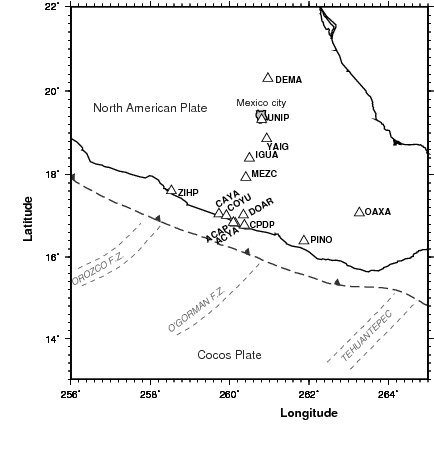
Figure 1: The Guerrero gap region of Mexico. The subduction zone studied in this paper meets the sea floor of the Pacific ocean along a nearly linear course called the Middle American Trench: it appears on this figure as a dashed line. The large triangles mark the locations of GPS stations that were used to record the 2006 Guerrero SSE.

Figure 1 shows locations where surface displacements have been recorded. Over time, some recording stations have closed while others have opened: it is therefore preferable not to use all these stations in the training step. Specifically, we will use measurements from the stations ACAP, ACYA, CAYA, COYU, CPDP, DEMA, DOAR, IGUA, MEZC, UNIP, YAIG. In effect, these will be the points $P_{j}$ in our computations, for $j=1,..,N$, and $N$ is equal to 11. We use a rectangular system of coordinates $x_{1},x_{2},x_{3}$ centered at ACAP: the $x_{1}$ direction runs West-East, the $x_{2}$ direction runs South-North, and the $x_{3}$ direction runs down-up. In effect, this assumes that the Earth is locally flat. Units for distances will be kilometers. Local geography is ignored, so $x_{3}=0$ at each of these 11 stations. The medium Lamé coefficients $\lambda$ and $\mu$ will be set to 1, which results in a Poisson ratio 0.25, a commonly agreed upon value for Earth’s rocks. We refer to [28, 30] for an account of how raw displacement data was collected day after day. The data was then completed and smoothed, as explained in [28]. The error bar on the data can be estimated by comparing the smoothed data to the raw data. Here we have to emphasize that finding the most optimal and accurate estimates of the average and the standard deviation of displacement fields is beyond the scope of our work. However, satisfactory estimates are easy to find and provide a good starting point for addressing the stochastic fault inverse problem. The effective maximum of $|\tilde{{\itbf u}}(P_{j})|$ is about 100 mm. The standard deviation on measurements of horizontal displacements can be estimated to .8 mm, and 2 mm for the standard deviation of vertical displacements. We will show in this section three test cases before covering the real world case. In the test cases, the surface points $P_{j}$ will be the same as the ones used in the real world data case. We simulated data and added gaussian noise with same covariance as the one estimated in the real world data case. In the test cases we made sure to set faults with depths that are consistent with what geophyscists expect to find in that region (in general, these depths are not deeper than 80 km, due to the thickness of Earth’s crust) and to produce surface displacements with the same order of magnitude as those observed for the 2007 Guerrero SSE.
In each case we set the center of the rectangle $R$ to be the average of the coordinates of $P_{j}$ weighted by $|\tilde{{\itbf u}}(P_{j})|$. The lengths of the sides of the rectangle $R$ can be set by first examining a large area which includes all the $P_{j}$s and then re-focusing it from a reconstructed ${\itbf h}$. Alternatively, the size of rectangle $R$ can be estimated by applying the quasi constant slip method presented in section 3.1 of [28].

6.1 First test case

In our first example, $\tilde{m}$ is such that $a=-0.3,\,b=-0.15,\,d=-14$. A sketch of the fault $\Gamma$, of the slip field $\tilde{{\itbf h}}$, and the resulting surface measurements $\tilde{{\itbf u}}(P_{j})$ is shown in Figure 2. After surface displacements were computed following formula (3.4), Gaussian noise with zero mean was added. We picked a covariance matrix with diagonal terms equal to $(.5\mbox{ mm})^{2}$ for horizontal displacements and $(1.5\mbox{ mm})^{2}$ for vertical displacements. In Figure 3 we show computed selected values of $C(i_{1},i_{2},i_{3})$ near ${\bf C}$ for different values of $\mathrm{{\bf Err}}$, see definitions 5.1 and (5.13). It is not possible to point to a single preferred value for $\mathrm{{\bf Err}}$, but we should expect it to be at least twice the standard deviation of the measurements. In Figure 3 we show selected values of $C(i_{1},i_{2},i_{3})$ for the relative error $\mathrm{{\bf Err}}/\|u^{(3N)}\|$ between 0.01 and 0.2. Since there is no preferred value of $\mathrm{{\bf Err}}$, we choose several possible ${\bf C}$: in this particular case $k\cdot 10^{-4}$, for $k=1..10$. In Figure 4 we show computed marginal distributions for the geometry parameters $a$, $b$, and $d$ for the value ${\bf C}=10^{-3}$ and three different assumed values of $\sigma_{hor}$ and $\sigma_{ver}$, the standard deviation for horizontal and vertical measurements.

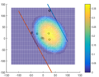
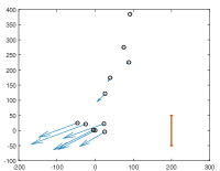
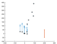
Figure 2: Test case 1. Top left: the fault $\Gamma$ and the slip field $\tilde{{\itbf h}}$. The red line is $x_{3}=-2$, the blue line is $x_{3}=-40$, on the plane $x_{3}=ax_{1}+bx_{2}+d$. The circles stand for the surface measurement points $P_{j}$. They appear on the map in Figure 1. Units for surface distances are kilometers. Color bar shows $|\tilde{{\itbf h}}|$, in meters. $\tilde{{\itbf h}}$ points in the direction of steepest ascent. The next two panels show the resulting surface displacements at the $P_{j}$s. The red line segment indicates the scale: 100 mm.

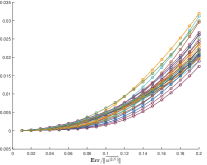
Figure 3: Test case 1. Examples of plots of $C(i_{1},i_{2},i_{3})$ against $\mathrm{{\bf Err}}/\|u^{(3N)}\|$.

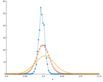
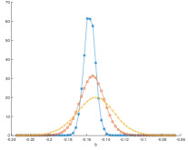
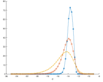
Figure 4: Test case 1. Computed marginal distributions for the geometry parameters $a$, $b$, and $d$. The blue star curve corresponds to the assumption $\sigma_{hor}=1,\sigma_{ver}=3$, the red circle curve corresponds to the assumption $\sigma_{hor}=2,\sigma_{ver}=6$, and the orange cross curve corresponds to the assumption $\sigma_{hor}=3,\sigma_{ver}=9$.

6.2 Second test case

In our second test, $\tilde{m}$ is such that $a=-0.3,b=0.15,d=-25$. The slip field for producing the surface data is sketched in Figure 5. This is a more challenging case since this field is non-convex. In addition, for this combination of geometry and slip field only a few points $P_{j}$ contribute valuable information for the surface displacement field. In theory, with continuous data on an open set of the surface $x_{3}=0$ this should not be a problem, but in practice, with a limited number of observation points our algorithm does not perform as well as previously. The most likely recovered values for $m$ are about $-0.2,\,0.1,\,-27$, this is not as close to the correct values as in the previous case. In Figure 7 we show the reconstructed slip field for this most likely geometry. Note how one of the two connected components of $\tilde{{\itbf h}}$ is better reconstructed than the other one.

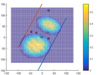
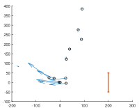
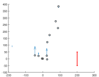
Figure 5: Test case 2. Legend is the same as in Figure 2.

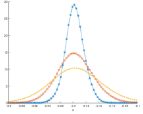
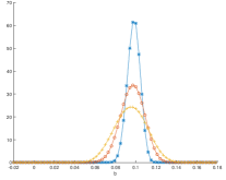
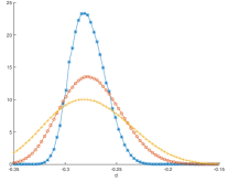
Figure 6: Test case 2: computed marginal distributions for the geometry parameters $a$, $b$, and $d$. Same caption as in Figure 4.

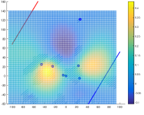
Figure 7: Test case 2. Reconstructed slip field.

6.3 Third test case

In our third test, $\tilde{m}$ is such that $a=0.1,b=-0.15,d=-24$. In this case we illustrate how (modest) modeling errors may impact the reconstruction algorithm. Here, the direction of slip is not in line with the direction of steepest ascent, while in the reconstruction step we wrongly assume that these two directions are the same. These two directions and the fault are sketched in Figure 8. In addition, noise was added to the surface measurements as in the previous two cases. In Figure 9 we show computed marginal distributions for the geometry parameters $a$, $b$, and $d$. The computed maximum likelihood for $m$ are achieved at .12, -.14, -20, so in this ”wrong model” case these values are not as close to the original values that were used to produce data as they were in the first test case.

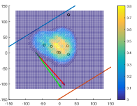
Figure 8: Test case 3. Legend is the same as in the top left panel of Figure 2. The direction of steepest ascent is indicated by the green arrow while the red arrow indicates the direction of slip.

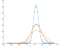
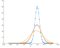
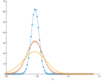
Figure 9: Test case 3: computed marginal distributions for the geometry parameters $a$, $b$, and $d$. Same caption as in Figure 4.

6.4 Application to the case of measured surface displacements during the 2007 SSE in Guerrero, Mexico

We now show the most interesting case as far as applications are concerned. We start from measurements relative to the 2007 SSE in Guerrero, Mexico, which were processed as described earlier: both ${\itbf u}(P_{j})$ and standard deviation on these measurements were estimated. We show in Figure 10 computed marginal distributions for the geometry parameters $a$, $b$, and $d$ for the constant ${\bf C}$ set to $6\cdot 10^{-4}$. Next we fix (approximate) most likely values for the geometry parameters $a,b,d$ to $-.13,\,-.19,\,-18$, and we compute expected slip on the fault and standard deviation: results are shown in Figure 11. Here we need to point out that once the geometry of the fault is fixed, we only need to solve a linear stochastic inverse problem: this is rather trivial since there is a linear relationship between the covariance matrix of the data and the covariance matrix of the slip on the field.
In the case of measured data, we can only validate our calculation by comparing our reconstructed fault to those offered by earlier studies: see [17, 22, 25] for the geometry of the fault (these studies were based on seismicity and gravity), [23, 24] for the profile of the slip on the fault, and [28, 30] for combined (deterministic) studies of simultaneous reconstruction of geometry and slip fields. In Figure 11, the computed line with depth $x_{3}=-2$ on the fault is shown in red. Note how close to the Middle American Trench sketched in Figure 1 this line is. With $\sigma_{hor}=1,\sigma_{ver}=3$, the standard deviations for $m$ are $0.020,\,0.023,\,1.7$, so the depth below ACAP is approximately between 16 and 20 km, and 50 km in the direction of steepest descent the depth is between 27 km and 33 km (these are plus or minus 1 standard deviation intervals). This is comparable and rather on the high side of depths found in other studies, see Figure 10 in [30].

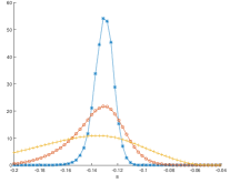
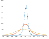
Figure 10: The 2007 Guerrero SSE. Computed marginal distributions for the geometry parameters $a$, $b$, and $d$. The blue star curve corresponds to the assumption that $\sigma_{hor}=.5,\sigma_{ver}=1.5$, the red circle curve corresponds to the assumption that $\sigma_{hor}=1,\sigma_{ver}=3$, and the orange cross curve corresponds to the assumption that $\sigma_{hor}=2,\sigma_{ver}=6$.

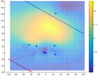
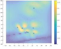
Figure 11: Computed average slip (left) and standard deviation (right) for the Guerrero 2007 SSE. Note the change of scale for the color bars between the two figures.

7 Appendix

The following two lemmas are needed for the proof of Theorem 4.1.

Lemma 7.1

Let ${\itbf h}^{disc}_{m,C}$ be the unique point where $F^{disc}_{m,C}$ achieves its minimum in ${\cal F}_{p}$. There are two positive constants $C_{0}$ and $C_{1}$ such that ${\itbf h}^{disc}_{m,C}$ is uniformly bounded in $H^{1}_{0}(R)$ for all $m$ in $B$, $p$ in $\mathbb{N}$, $N$ in $\mathbb{N}$ and $C$ such that $C_{0}N^{-\beta}<C<C_{1}$.

Proof:
With $\tilde{{\itbf h}}$ as in the statement of Theorem 3.1, let $\tilde{{\itbf h}}_{p}$ be the orthogonal projection of $\tilde{{\itbf h}}$ on ${\cal F}_{p}$. As

$$F^{disc}_{m,C}({\itbf h}_{m,C}^{disc})\leq F^{disc}_{m,C}(\tilde{{\itbf h}}_{p}),$$

we have

$$C\int_{R}|{\itbf h}_{m,C}^{disc}|^{2}\leq\sum_{j=1}^{N}C^{\prime}(j,N)|{\cal C}^{-\frac{1}{2}}(A_{m}\tilde{{\itbf h}}_{p}-\tilde{{\itbf u}})(P_{j})|^{2}+C\int_{R}|\tilde{{\itbf h}}_{p}|^{2}.$$ (7.1)

Since $\|\tilde{{\itbf h}}_{p}\|\leq\|\tilde{{\itbf h}}\|$, given that $A_{m}$ is continuous in $m$, $B$ is compact, and $A_{m}$ continuously maps $H^{1}_{0}(R)$ into smooth functions on $V$, by (4.2),

$$\sum_{j=1}^{N}C^{\prime}(j,N)|{\cal C}^{-\frac{1}{2}}(A_{m}\tilde{{\itbf h}}_{p}-\tilde{{\itbf u}})(P_{j})|^{2}=O(N^{-\beta}),$$

thus

$$\int_{R}|{\itbf h}_{m,C}^{disc}|^{2}=O(1+C^{-1}N^{-\beta}),$$ (7.2)

uniformly for all $m$ in $B$, $p$ in $\mathbb{N}$, $N$ in $\mathbb{N}$ and $C>0$.

Lemma 7.2

Assume that $\tilde{{\itbf u}}=A_{\tilde{m}}\tilde{{\itbf h}}$ for some $\tilde{m}$ in $B$ and some $\tilde{{\itbf h}}$ in $H_{0}^{1}(R)$. Fix $m$ in $B$ such that $m\neq\tilde{m}$ and $M>0$. Set

$$\gamma=\inf_{{\itbf g}\in H^{1}_{0}(R),\|{\itbf g}\|\leq M}\int_{V}|{\cal C}^{-\frac{1}{2}}(A_{m}{\itbf g}-\tilde{{\itbf u}})|^{2}.$$

Then $\gamma>0$.

Proof:
Arguing by contradiction, assume that $\gamma=0$. Then there is a sequence ${\itbf g}_{n}$ in $H^{1}_{0}(R)$ such that $\|{\itbf g}_{n}\|\leq M$ and $\int_{V}|{\cal C}^{-\frac{1}{2}}(A_{m}{\itbf g}_{n}-\tilde{{\itbf u}})|^{2}$ converges to zero as $n\rightarrow\infty$. A subsequence of ${\itbf g}_{n}$ is weakly convergent in $H^{1}_{0}(R)$ to some ${\itbf h}^{*}$. It will still be denoted by ${\itbf g}_{n}$ for the sake of simpler notations. As the operator $A_{m}$ is compact, we find at the limit that $\int_{V}|{\cal C}^{-\frac{1}{2}}(A_{m}{\itbf h}^{*}-\tilde{{\itbf u}})|^{2}=0$. Since $m\neq\tilde{m}$, this contradicts uniqueness Theorem 2.2.

Proof of Theorem 4.1:
Arguing by contradiction, assume that there exist an $\eta>0$ and three sequences $N_{n}$ in $\mathbb{N}$, $p_{n}$ in $\mathbb{N}$, and $C_{n}$ in $(0,1)$ such that $N_{n}\rightarrow\infty$, $p_{n}\rightarrow\infty$ and $C_{n}\rightarrow 0$ while $C_{n}^{-1}N_{n}^{-\beta}$ is bounded above and denoting

$$f^{disc}_{C_{n}}(m_{n})=\min_{m\in B}\min_{{\itbf g}\in{\cal F}_{p_{n}}}\sum_{j=1}^{N_{n}}C^{\prime}(j,N_{n})|{\cal C}^{-\frac{1}{2}}(A_{m}{\itbf g}-\tilde{{\itbf u}})(P_{j})|^{2}+C_{n}\int_{R}|\nabla{\itbf g}|^{2},$$

we have that $|m_{n}-\tilde{m}|>\eta$. As $B$ is compact, after possibly extracting a subsequence, we may assume that $m_{n}$ converges to some $m^{*}$ in $B$, with $m^{*}\neq\tilde{m}$. Since $C_{n}$ tends to zero, applying Theorem 3.1, there is a sequence $m_{n}^{\prime}$ which converges to $\tilde{m}$ and such that

$$\int_{V}|{\cal C}^{-\frac{1}{2}}(A_{m_{n}^{\prime}}{\itbf h}_{m_{n}^{\prime},C_{n}}-\tilde{{\itbf u}})|^{2}\rightarrow 0,\quad{\itbf h}_{m_{n}^{\prime},C_{n}}\rightarrow\tilde{{\itbf h}}$$ (7.3)

where $\displaystyle F_{m_{n}^{\prime},C_{n}}({\itbf h}_{m_{n}^{\prime},C_{n}})=\min_{{\itbf g}\in H^{1}_{0}(R)}F_{m_{n}^{\prime},C_{n}}({\itbf g})$, so $F_{m_{n}^{\prime},C_{n}}({\itbf h}_{m_{n}^{\prime},C_{n}})$ converges to zero. Fix $\epsilon>0$. Set $\displaystyle F_{m_{n},C_{n}}^{disc}({\itbf h}_{m_{n},C_{n}}^{disc})=\min_{{\itbf g}\in{\cal F}_{p_{n}}}F^{disc}_{m_{n},C_{n}}({\itbf g})$. Let ${\itbf h}_{m_{n}^{\prime},C_{n},p}$ be the orthogonal projection of ${\itbf h}_{m_{n}^{\prime},C_{n}}$ on ${\cal F}_{p}$. We first note that the convergence of ${\itbf h}_{m_{n}^{\prime},C_{n}}$ to ${\itbf h}$ implies that ${\itbf h}_{m_{n}^{\prime},C_{n},p}$ converges to ${\itbf h}_{m_{n}^{\prime},C_{n}}$ as $p\rightarrow\infty$, uniformly in $n$. Thus, using minimality of ${\itbf h}_{m_{n},C_{n}}^{disc}$,

$$F^{disc}_{m_{n},C_{n}}({\itbf h}_{m_{n},C_{n}}^{disc})\leq F^{disc}_{m_{n}^{\prime},C_{n}}({\itbf h}_{m_{n}^{\prime},C_{n},p_{n}})\leq F^{disc}_{m_{n}^{\prime},C_{n}}({\itbf h}_{m_{n}^{\prime},C_{n}})+\epsilon,$$

for all $n$ large enough. Using again the boundedness of ${\itbf h}_{m_{n}^{\prime},C_{n}}$, we can write that for all $n$ large enough,

$$F^{disc}_{m_{n}^{\prime},C_{n}}({\itbf h}_{m_{n}^{\prime},C_{n}})\leq F_{m_{n}^{\prime},C_{n}}({\itbf h}_{m_{n}^{\prime},C_{n}})+\epsilon,$$

and since $F_{m_{n}^{\prime},C_{n}}({\itbf h}_{m_{n}^{\prime},C_{n}})$ converges to zero we infer that for all $n$ large enough,

$$F^{disc}_{m_{n},C_{n}}({\itbf h}_{m_{n},C_{n}}^{disc})\leq 3\epsilon.$$ (7.4)

By Lemma 7.1, ${\itbf h}_{m_{n},C_{n}}^{disc}$ is bounded by a constant that only depends on $\tilde{{\itbf h}}$, so for all large enough $n$

$$\int_{V}|{\cal C}^{-\frac{1}{2}}(A_{m^{*}}{\itbf h}_{m_{n},C_{n}}^{disc}-\tilde{{\itbf u}})|^{2}\leq 4\epsilon.$$ (7.5)

This contradicts Lemma 7.2 for $\epsilon$ small enough.

Proof of Proposition 5.1:
First we combine the exponentials in (5.3) and (5.4) to find

$$\rho(\tilde{{\itbf u}}_{meas}|m,{\itbf g})\rho_{{\cal F}}({\itbf g})\propto\exp(-\frac{1}{2}\sum_{j=1}^{N}C^{\prime}(j,N)|({\cal C}^{-\frac{1}{2}}A_{m}{\itbf g}-\tilde{{\itbf u}}_{meas})(P_{j})|^{2}-\frac{1}{2}C\int_{R}|\nabla{\itbf g}|^{2}),$$ (7.6)

which needs to be integrated in ${\itbf g}$ over ${\cal F}_{p}$. With ${\itbf h}^{disc}_{m,C}$ is as in (4.3) and the adjoint defined as in the statement of Proposition 5.1, ${\itbf h}^{disc}_{m,C}$ satisfies

$$A_{m}^{\prime}{\cal D}^{2}A_{m}{\itbf h}^{disc}_{m,C}+C{\itbf h}^{disc}_{m,C}=A_{m}^{\prime}{\cal D}^{2}\tilde{{\itbf u}}_{meas}.$$

Setting ${\itbf g}={\itbf h}^{disc}_{m,C}+{\itbf h}$, it follows that

$$\|{\cal D}A_{m}{\itbf g}-{\cal D}\tilde{{\itbf u}}_{meas}\|^{2}+C\|{\itbf g}\|^{2}=\|{\cal D}A_{m}{\itbf h}^{disc}_{m,C}-{\cal D}\tilde{{\itbf u}}\|^{2}+C\|{\itbf h}^{disc}_{m,C}\|^{2}+\|{\cal D}A_{m}{\itbf h}\|^{2}+C\|{\itbf h}\|^{2},$$

Next we set $q=\dim{\cal F}_{p}$ and we introduce an orthonormal basis ${\itbf e}_{1},...,{\itbf e}_{q}$ of ${\cal F}_{p}$ which diagonalizes $A_{m}^{\prime}{\cal D}^{2}A_{m}$. Let $\mu_{j}^{2}$ be such that $A_{m}^{\prime}{\cal D}^{2}A_{m}{\itbf e}_{j}=\mu_{j}^{2}{\itbf e}_{j}$. We can now integrate $\exp(-\frac{1}{2}\|{\cal D}A_{m}{\itbf h}\|^{2}-\frac{1}{2}C\|{\itbf h}\|^{2})$ for ${\itbf h}$ over ${\cal F}_{p}$ by just rotating the natural basis of ${\cal F}_{p}$ to the orthonormal basis ${\itbf e}_{1},...,{\itbf e}_{q}$ to obtain

$$\prod_{j=1}^{q}\int_{-\infty}^{\infty}\exp(-\frac{1}{2}(\mu_{j}^{2}+C)t^{2})dt=\prod_{j=1}^{q}\frac{\sqrt{2\pi}}{\sqrt{\mu_{j}^{2}+C}}=\frac{1}{\sqrt{\det((2\pi)^{-1}(A_{m}^{\prime}{\cal D}^{2}A_{m}+CI_{q}))}}.$$

Proof of Lemma 5.1:
Due to the minimization property (5.11) it is clear that $\|{\cal D}(Ag^{(p)}-u^{(3N)})\|\leq\|{\cal D}u^{(3N)}\|$ for all $C>0$. As ${\cal D}(Ag^{(p)}-v^{(3N))}$ is orthogonal to ${\cal D}(u^{(3N)}-v^{(3N)})$, by the Pythagorean theorem,

$$\|{\cal D}(Ag^{(p)}-u^{(3N)})\|^{2}=\|{\cal D}(Ag^{(p)}-v^{(3N)})\|^{2}+\|{\cal D}(u^{(3N)}-v^{(3N)})\|^{2},$$ (7.7)

so $\|{\cal D}(Ag^{(p)}-u^{(3N)})\|\geq\|{\cal D}(u^{(3N)}-v^{(3N)})\|$. If we assume that $\|{\cal D}(Ag^{(p)}-u^{(3N)})\|=\|{\cal D}u^{(3N)}\|$ for some $C>0$, then the minimum of (5.11) is achieved for $g^{(p)}=0$, so $A^{\prime}{\cal D}^{2}u^{(3N)}=0$ due to (5.12) which contradicts the assumption that $v^{(3N)}$ is non-zero. If we assume that $\|{\cal D}(Ag^{(p)}-u^{(3N)})\|=\|{\cal D}(u^{(3N)}-v^{(3N)})\|$ for some $C>0$, then $\|{\cal D}(Ag^{(p)}-v^{(3N)})\|=0$ due to the Pythagorean theorem, so $C(D^{\prime}D+E^{\prime}E)g^{(p)}=A^{\prime}{\cal D}^{2}(u^{(3N)}-v^{(3N)})$, but $A^{\prime}{\cal D}^{2}(u^{(3N)}-v^{(3N)})$ by definition of $v^{(3N)}$, thus $g^{(p)}=0$ due to (5.12), leading to a contradiction.
In [30], Appendix B, we showed how $D$ and $E$ can be chosen assuming that we use a regular grid on $R$. For that particular choice, $\|D\|$ and $\|E\|$ are equal to 2 while $\|D^{-1}\|$ and $\|E^{-1}\|$ are bounded by $\sqrt{q}$. (we used $q$ for an upper bound for $\|D\|$ and $\|E\|$ but that bound can be improved to $\sqrt{q}$ by observing that the block matrix $M$ defined in appendix B of [30] is the sum of the identity and a $m$- nilpotent matrix with norm 1, where $m=\sqrt{q}$). As for any $x$ in $\mathbb{R}^{q}$

$$x^{T}(A^{\prime}{\cal D}^{2}Ag^{(p)}+C(D^{\prime}D+E^{\prime}E))x\geq C\|Dx\|^{2}+C\|Ex\|^{2}\geq\frac{4C}{q}\|x\|^{2},$$ (7.8)

$(A^{\prime}{\cal D}^{2}A+C(D^{\prime}D+E^{\prime}E))^{-1}$ exists for all $C>0$ and is a continuous function of $C$. Since $g^{(p)}$ solves (5.12), $g^{(p)}$ and $\|{\cal D}(Ag^{(p)}-v^{(3N)})\|$ are also continuous functions of $C$ in $(0,\infty)$.
Left multiplying (5.12) by $g^{p}$ and applying the Cauchy Schwartz inequality we find

$$\|{\cal D}Ag^{(p)}\|^{2}+C\|Dg^{(p)}\|^{2}+C\|Eg^{(p)}\|^{2}\leq\|{\cal D}u^{(3N)}\|\|{\cal D}Ag^{(p)}\|,$$

thus

$$\frac{1}{2}\|{\cal D}Ag^{(p)}\|^{2}+C\|Dg^{(p)}\|^{2}+C\|Eg^{(p)}\|^{2}\leq\frac{1}{2}\|{\cal D}u^{(3N)}\|^{2}.$$

Recalling (7.8) we find

$$\|g^{(p)}\|^{2}\leq\frac{q}{8C}\|{\cal D}u^{(3N)}\|^{2},$$

thus $\displaystyle\lim_{C\rightarrow\infty}g^{(p)}=0$, so $\displaystyle\lim_{C\rightarrow\infty}\|{\cal D}(Ag^{(p)}-u^{(3N)})\|=\|{\cal D}u^{(3N)}\|$.
To find the limit of $Ag^{(p)}-u^{(3N)}$ as $C$ tends to zero we first recall that $A^{\prime}{\cal D}^{2}(u^{(3N)}-v^{(3N)})=0$. By definition there is an $x$ in $\mathbb{R}^{p}$ such that ${\cal D}Ax={\cal D}v^{(3N)}$. From (5.12),

$$A^{\prime}{\cal D}^{2}A(g^{(p)}-x)+C(D^{\prime}D+E^{\prime}E)(g^{(p)}-x)=-C(D^{\prime}D+E^{\prime}E)x$$

thus

$$\|{\cal D}A(g^{(p)}-x)\|^{2}+\frac{1}{2}C\|D(g^{(p)}-x)\|^{2}+\frac{1}{2}C\|E(g^{(p)}-x)\|^{2}\leq\frac{1}{2}C\|Dx\|^{2}+\frac{1}{2}C\|Ex\|^{2},$$

so $\displaystyle\lim_{C\rightarrow 0}\|{\cal D}A(g^{(p)}-x)\|=0$ and by the Pythagorean formula (7.7)

$$\lim_{C\rightarrow 0}\|{\cal D}(Ag^{(p)}-u^{(3N)})\|=\|{\cal D}(u^{(3N)}-v^{(3N)})\|.$$

References

- [1] Habib Ammari, Josselin Garnier, Hyonbae Kang, Won-Kwang Park, and Knut Solna. Imaging schemes for perfectly conducting cracks. SIAM Journal on Applied Mathemat- ics, 71(1):68-91, 2011.
- [2] Eiichiro Araki, Demian M Saffer, Achim J Kopf, Laura M Wallace, Toshinori Kimura, YuyaMachida, Satoshi Ide, Earl Davis, IODP Expedition, et al. Recurring and triggered slow-slip events near the trench at the nankai trough subduction megathrust. Science, 356(6343):1157-1160, 2017.
- [3] Brian F Atwater, Alan R Nelson, John J Clague, Gary A Carver, David K Yamaguchi, Peter T Bobrowsky, Joanne Bourgeois, Mark E Darienzo, Wendy C Grant, Eileen Hemphill-Haley, et al. Summary of coastal geologic evidence for past great earthquakes at the cascadia subduction zone. Earthquake spectra, 11(1):1-18, 1995.
- [4] Elena Beretta, Elisa Francini, Eunjoo Kim, and June-Yub Lee. Algorithm for the determination of a linear crack in an elastic body from boundary measurements. Inverse Problems, 26(8):085015, 2010.
- [5] Elena Beretta, Elisa Francini, and Sergio Vessella. Determination of a linear crack in an elastic body from boundary measurements-lipschitz stability. SIAM Journal on Mathematical Analysis, 40(3):984-1002, 2008.
- [6] Liliana Borcea, George Papanicolaou, and Chrysoula Tsogka. Theory and applications of time reversal and interferometric imaging. Inverse Problems, 19(6):S139, 2003.
- [7] Cristian Dascalu, Ioan R Ionescu, and Michel Campillo. Fault niteness and initiation of dynamic shear instability. Earth and Planetary Science Letters, 177(3):163-176, 2000.
- [8] H. Dragert, K. Wang, and G. Rogers. Geodetic and seismic signatures of episodic tremor and slip in the northern Cascadia subduction zone. Earth Planets and Space, 56(12):1143-1150, 2004.
- [9] H. Dragert, K. L. Wang, and T. S. James. A silent slip event on the deeper Cascadia subduction interface. Science, 5521:1525-1528, 2001.
- [10] Avner Friedman and Michael Vogelius. Determining cracks by boundary measurements, 1989. http://conservancy.umn.edu/bitstream/handle/11299/4926/476.pdf.
- [11] I. Gohberg and M. G. Krein. Introduction to the theory of linear nonselfadjoint operators. American Mathematical Soc., 18, 1969.
- [12] Gene H Golub, Michael Heath, and Grace Wahba. Generalized cross-validation as a method for choosing a good ridge parameter. Technometrics, 21(2):215-223, 1979.
- [13] Per Christian Hansen. Analysis of discrete ill-posed problems by means of the L-curve. SIAM review, 34(4):561-580, 1992.
- [14] Ioan R Ionescu and Darko Volkov. Earth surface effects on active faults: An eigenvalue asymptotic analysis. Journal of Computational and Applied Mathematics, 220(1):143- 162, 2008.
- [15] Jari Kaipio and Erkki Somersalo. Statistical and computational inverse problems, volume 160. Springer Science & Business Media, 2006.
- [16] Misha E Kilmer and Dianne P O’Leary. Choosing regularization parameters in iterative methods for ill-posed problems. SIAM Journal on matrix analysis and applications, 22(4):1204-1221, 2001.
- [17] V. Kostoglodov, W. Bandy, J. Dominguez, and M. Mena. Gravity and seismicity over the Guerrero seismic gap, Mexico. Geophys. Res. Lett., 23(23):3385-3388, 1996.
- [18] Rainer Kress, V Maz’ya, and V Kozlov. Linear integral equations, volume 17. Springer, 1989.
- [19] John M Lee and Gunther Uhlmann. Determining anisotropic real-analytic conductivities by boundary measurements. Communications on Pure and Applied Mathematics, 42(8):1097-1112, 1989.
- [20] Youssef M Marzouk, Habib N Najm, and Larry A Rahn. Stochastic spectral methods for efficient bayesian solution of inverse problems. Journal of Computational Physics, 224(2):560-586, 2007.
- [21] Y. Okada. Internal deformation due to shear and tensile faults in a half-space. Bulletin of the Seismological Society of America, vol. 82 no. 2:1018-1040, 1992.
- [22] J. F. Pacheco and S. K. Singh. Seismicity and state of stress in Guerrero segment of the Mexican subduction zone. J. Geophys. Res., 115, 2010.
- [23] M. Radiguet, F. Cotton, M. Vergnolle, M. Campillo, B. Valette, V. Kostoglodov, and N. Cotte. Spatial and temporal evolution of a long term slow slip event: the 2006 Guerrero Slow Slip Event. Geophysical Journal International, 2010.
- [24] M. Radiguet, F. Cotton, M. Vergnolle, M. Campillo, A. Walpersdorf, N. Cotte, , and V. Kostoglodov. Slow slip events and strain accumulation in the Guerrero gap, Mexico. JOURNAL OF GEOPHYSICAL RESEARCH, 2012.
- [25] G. Suarez, T. Monfret, G. Wittlinger, and C. David. Geometry of subduction and depth of the seismogenic zone in the Guerrero gap, Mexico. Nature, 345(6273):336-338, 1990.
- [26] John Sylvester and Gunther Uhlmann. A global uniqueness theorem for an inverse boundary value problem. Annals of mathematics, pages 153-169, 1987.
- [27] D. Volkov. A double layer surface traction free green’s tensor. SIAM J. APPL. MATH., 69 (5):1438-1456, 2009.
- [28] D. Volkov, C. Voisin, and Ionescu I.R. Determining fault geometries from surface displacements. Pure and Applied Geophysics, 174(4):1659-1678, 2017.
- [29] Darko Volkov. An eigenvalue problem for elastic cracks in free space. Mathematical Methods in the Applied Sciences, 33(5):607-622, 2010.
- [30] Darko Volkov, Christophe Voisin, and Ioan Ionescu. Reconstruction of faults in elastic half space from surface measurements. Inverse Problems, 33(5), 2017.