Modeling and identification of uncertain-input systems

Abstract

In this work, we present a new class of models, called uncertain-input models, that allows us to treat system-identification problems in which a linear system is subject to a partially unknown input signal. To encode prior information about the input or the linear system, we use Gaussian-process models. We estimate the model from data using the empirical Bayes approach: the input and the impulse responses of the linear system are estimated using the posterior means of the Gaussian-process models given the data, and the hyperparameters that characterize the Gaussian-process models are estimated from the marginal likelihood of the data. We propose an iterative algorithm to find the hyperparameters that relies on the EM method and results in simple update steps. In the most general formulation, neither the marginal likelihood nor the posterior distribution of the unknowns is tractable. Therefore, we propose two approximation approaches, one based on Markov-chain Monte Carlo techniques and one based on variational Bayes approximation. We also show special model structures for which the distributions are treatable exactly. Through numerical simulations, we study the application of the uncertain-input model to the identification of Hammerstein systems and cascaded linear systems. As part of the contribution of the paper, we show that this model structure encompasses many classical problems in system identification such as classical PEM, Hammerstein models, errors-in-variables problems, blind system identification, and cascaded linear systems. This allows us to build a systematic procedure to apply the algorithms proposed in this work to a wide class of classical problems.

1 Introduction

In most system identification problems, the input signal—that is, the independent variable—is perfectly known [24]. Often, the input signal is the result of an identification experiment, where a signal with certain characteristics is designed and applied to the system to measure its response. However, in some applications, the hypothesis that the input signal is known may be too restrictive. In this work, we propose a new model structure that accounts for partial knowledge about the input signal and we show how many classical system identification problems can be seen as problems of identifying instances of this model structure.

The proposed model structure, which we call uncertain-input model, is composed of a linear time-invariant dynamical system (the linear system) and of a signal of which partial information is available (the unknown input). In the next section, we characterize formally the unknown input; before that, we give some examples of classical models that can be seen as uncertain-input models. The Hammerstein model is a cascade composition of a static nonlinear function followed by a linear time-invariant dynamical system [3, 20, 39]. In the Hammerstein model, the (perfectly known) input signal passes through the unknown static nonlinear function. After the nonlinear transformation, the signal which is fed to the linear system, is completely unknown. However, some characteristics of the signal may be known; for instance, we may known that the nonlinear function is smooth or we may have a set of candidate basis functions to choose among. Another instance of a model where the input is not perfectly known is the errors-in-variables model [45]. In the errors-in-variables formulation, the input in known up to noisy measurements. The noise in the input introduces many difficulties and special techniques have been developed to deal with it [43, 44]. Closely related to errors-in-variables models, blind system identification methods are used when the input signal is completely unknown [1]. These are particularly useful in telecommunications, image reconstruction, and biomedical applications [31, 30, 27]. Blind system identification problems are generally ill posed, and certain assumptions on the input signal are needed to recover a solution [2]. Similar to blind problems are the problems of system identification with missing data. In these cases, the missing data are estimated, together with a description of the system, by making hypotheses on the mechanism that generated the missing data [47, 26, 34, 42, 23].

In all the applications we have outlined, we can identify the common thread of a linear system fed by a signal about which we have limited prior information. This leads us naturally to consider a Bayesian framework where we can use prior distributions to encode beliefs about the unknown quantities [8, Section 2.4]. Within the vast framework of Bayesian methods, we concentrate on Gaussian processes [38]. These enable us to compute many quantities in closed form and to reason about identification in terms of a limited number of sufficient statistics. For these reasons, Gaussian-process modeling has become a popular approach in system identification [36, 17, 46]. Although Gaussian processes are typically analytically convenient, the structure of the uncertain-input problem leads to an intractable inference problem: even though we model the system and the input as Gaussian processes, the output of the system depends on their convolution and therefore does not admit a Gaussian description. To perform the inference—that is find the posterior distribution of the unknowns given the observations—we need approximation methods. We propose two different approximation methods for the posterior distribution of the unknowns: one Markov Chain Monte Carlo (MCMC, see [19]) method and one variational approximation [6] method. In the MCMC method, we use the Gibbs sampler [18] to draw particles from the posterior distribution and we approximate expectations as averages computed with the particles. In the variational method, we find the factorized distribution that best approximates the posterior distribution in Kullback-Leibler distance.

To give flexibility to the model, we allow the Gaussian priors to depend on certain parameters (called hyperparameters) that need to be estimated from data together with the measurement noise variances. To estimate these parameters, we use the empirical Bayes method which requires maximizing the marginal distribution of the data (sometimes called evidence, see [25]). To this end, we propose an iterative algorithm based on the Expectation-Maximization (EM) method [14]. The EM method alternates between the computation of the expected value of the joint likelihood of the data, of the unknown system, and of the input (E-step), and the maximization of this expected value with respect to the unknown parameters (M-step). We show that the E-step can be computed using the same approximations of the posterior distributions that are used in the inference and that the M-step consists in a series of simple and independent optimization problems that can be solved easily.

As mentioned above, the uncertain-input model encompasses several classical model structures that have been object of research in the system-identification community for decades. Two important contributions of this work are as follows.

1. We unify the problems of identifying systems that are usually regarded as belonging to different model classes into a single identification framework.

2. We formalize a method to apply the new tools of Gaussian processes and Bayesian inference to classical system identification problems.

To support the validity of the proposed methods, we present identification experiments on synthetic datasets of cascaded linear systems and of Hammerstein systems.

1.1 Notation

The notation $[A]{}_{i,j}$ indicates the element of matrix $A$ in position $i,j$ (single subscripts are used for vectors). “$\mathrm{T}_{N\times n}(v)$” denotes the $N$ by $n$ lower-triangular Toeplitz matrix of the $m$ dimensional vector $v$:

$$\mathinner{\left[\mathrm{T}_{N\times n}(v)\right]}_{i,j}=\begin{cases}v_{i-j+1}&0\leq i-j+1\leq m\\ 0&\text{otherwise}\end{cases}$$ (1)

If $v$ is a vector, then $V$ is the $N$ by $N$ Toeplitz matrix whose elements are given by $v$. The notation “$\|a\|^{2}_{M}$” is shorthand for $a^{T}Ma$. The notation “$\mathcal{N}(\alpha,\Sigma)$” indicates the Gaussian distribution with mean vector $\alpha$ and covariance matrix $\Sigma$. The notation “$\mathcal{GP}(\mu,\Sigma)$” indicate a Gaussian process with mean function $\mu$ and covariance function $\Sigma$. Random variables and their realizations have the same symbol. The notation “$x;\theta$” indicates that the random variable $x$ depends on the parameter $\theta$. If $x$ is a random variable, $\mathrm{p}(x)$ denotes its density. The symbol “$\cong$” indicates equality up to an additive constant and “$\delta$” is the Dirac density.

2 Uncertain-input systems

In this work, we propose a new model structure called the uncertain-input model. Consider the block scheme in Figure 1. Many system identification tasks can be formulated as the identification of a linear system $S$, subject to an input sequence $\{w_{t}\}$. In this work, we consider problems in which we have partial information about the input sequence, and this partial information depends on the specific problem at hand.

Figure 1: A block scheme of the general uncertain input system.

We assume that the linear system $S$ is time invariant, stable, and causal. Therefore, it is uniquely described by the sequence $\{g_{t}\}$ of its impulse response samples, and the output of the system generated by an input $\{w_{t}\}$ can be represented as the discrete convolution of the system impulse response with the input signal—that is, at time $t$, the measurements of the output can be written as the noise-corrupted discrete convolution

$$y_{t}=\mathinner{\left(w\ast g\right)}_{t}+\varepsilon_{t},$$ (2)

where $\{\varepsilon_{t}\}$ is a stochastic process that describes additive measurement noise, and where “$\ast$” denotes the discrete time convolution

$$\mathinner{\left(w\ast g\right)}_{t}=\sum_{k=1}^{\infty}g_{k}w_{t-k}.$$ (3)

In the uncertain-input model, we consider that the input signal is measured with additive white noise described by a stochastic processes $\{\eta_{t}\}$. This assumption allows us to write, for the input measurements, the model

$$v_{t}=w_{t}+\eta_{t}.$$ (4)

We assume that the noise processes $\{\eta_{t}\}$ and $\{\varepsilon_{t}\}$ are independent Gaussian white-noise processes. This means that every noise sample has a Gaussian distribution,

$$\eta_{t}\sim\mathcal{N}(0,\sigma_{v}^{2}),\quad\varepsilon_{t}\sim\mathcal{N}(0,\sigma_{y}^{2}),$$ (5)

and that $\varepsilon_{t}$ is independent of $\varepsilon_{s}$, for $s\neq t$, and of $\eta_{s}$ for any $s$. To allow for models where some observations are missing, we assume infinite variance for those noise components that correspond to the missing samples.

To encode the prior information we have about the input signal and about the linear system, we use Gaussian process models. We model the unknown input signal and the impulse response of the linear system as a realization of a joint Gaussian processes with suitable mean and covariance functions,

$$\mathinner{\Biggl{[}\begin{matrix}w\\ g\end{matrix}\Biggr{]}}\!\!\sim\!\mathcal{GP}\!\mathinner{\left(\!\!\mathinner{\Biggl{[}\begin{matrix}\mu_{w}(\cdot;\theta)\\ \mu_{g}(\cdot;\rho)\end{matrix}\Biggr{]}}\!\!,\!\mathinner{\Biggl{[}\begin{matrix}K_{w}(\cdot;\theta)&{K_{gw}(\cdot,\cdot;\rho,\theta)}^{T}\\ K_{gw}(\cdot,\cdot;\rho,\theta)&K_{g}(\cdot,\cdot;\rho)\end{matrix}\Biggr{]}}\right)}\!.$$ (6)

The mean functions of the Gaussian processes, $\mu_{g}(\cdot\,;\theta)$ and $\mu_{w}(\cdot\,;\rho)$, may depend on the parameter vectors $\theta$ and $\rho$, called hyperparameter vectors, which can be used to shape the prior information to the specific application. The same goes for the covariance functions $K_{w}(\,\cdot\,,\,\cdot\,;\theta)$, $K_{g}(\,\cdot\,,\,\cdot\,;\rho)$, and $K_{gw}(\,\cdot\,,\,\cdot\,;\rho,\theta)$ which may depend on (possibly different) hyperparameters.

For notational convenience, we present the explicit computations in the case of independent Gaussian process models for $g$ and $w$—that is, we consider the case where

$$\begin{split}w&\sim\mathcal{GP}\big{(}\mu_{w}(\,\cdot\,\,;\theta),K_{w}(\,\cdot\,,\,\cdot\,;\theta)\big{)},\\ g&\sim\mathcal{GP}\big{(}\mu_{g}(\,\cdot\,;\rho),K_{g}(\,\cdot\,,\,\cdot\,;\rho)\big{)},\end{split}$$ (7)

and the cross-covariance of processes is zero. However, all results we show hold also in the more general case.

We assume that we have collected $N$ measurements of the processes $\{v_{t}\}$ and $\{y_{t}\}$ and, for sake of simplicity, we also assume that $w_{t}=0$ for $t<0$ (see [41] for a way to extend the proposed framework to unknown initial conditions). From (2), we see that the output measurements only depend on the values of the impulse response at the discrete time instants $t=1,2,\ldots,N$; therefore, we can consider the joint distribution of the samples $g_{t}$ for $t=1,2,\ldots,N$. From the Gaussian process model (7), we have that, if we collect the samples of $\{g_{t}\}$ into an $N$-dimensional column vector $g$, this vector has a joint Gaussian distribution given by

$$g\sim\mathcal{N}\big{(}\mu_{g}(\rho),K_{g}(\rho)\big{)},$$ (8)

where we have defined the mean vector and the covariance matrix induced by (7) as

$${\big{[}\mu_{g}(\rho)\big{]}}_{j}\mathrel{\mathop{\mathchar 58\relax}}=\mu_{g}(j\,;\rho),\quad{\big{[}K_{g}(\rho)\big{]}}_{i,j}\mathrel{\mathop{\mathchar 58\relax}}=K_{g}(i,j\,;\rho).$$ (9)

From (4) and (2), we have that the $N$ measurements of the input and output only depend on the samples $w_{t}$ for $t=1,\ldots,N$; therefore, we can consider the joint distribution of these samples, collected in an $N$-dimensional vector $w$. This distribution is Gaussian, and it is given by

$$w\sim\mathcal{N}\big{(}\mu_{w}(\theta),K_{w}(\theta)\big{)},$$ (10)

where we have defined the mean vector and the covariance matrix induced by (7) as

$${\big{[}\mu_{w}(\theta)\big{]}}_{j}\mathrel{\mathop{\mathchar 58\relax}}=\mu_{w}(j\,;\theta),\quad{\big{[}K_{w}(\theta)\big{]}}_{i,j}\mathrel{\mathop{\mathchar 58\relax}}=K_{w}(i,j\,;\theta).$$ (11)

Assembling the models for the different components, given by (2), (4), (5), (8), and (10), we arrive at the following definition of the uncertain-input model:

$$\left\{\begin{aligned} y&=Wg+\varepsilon\\ v&=w+\eta\\ g&\sim\mathcal{N}\big{(}\mu_{g}(\rho),K_{g}(\rho)\big{)}\\ w&\sim\mathcal{N}\big{(}\mu_{w}(\theta),K_{w}(\theta)\big{)}\\ \varepsilon&\sim\mathcal{N}\big{(}0,\sigma_{y}^{2}I_{N}\big{)}\\ \eta&\sim\mathcal{N}\big{(}0,\sigma_{v}^{2}I_{N}\big{)}\\ g,\,&w,\,\varepsilon,\,\eta\text{ mutually independent}\end{aligned}\right.$$ (12)

where we have collected the output measurements $\{y_{t}\}$ in a vector $y$ and where $\varepsilon$ and $\eta$ are the vectors of the first $N$ input and output noise samples. The matrix $W$ is the $N\times N$ Toeplitz matrix of the input, $W\mathrel{\mathop{\mathchar 58\relax}}=\mathrm{T}_{N\times N}(w)$, which represents the discrete-time convolution (3) as the product $Wg$. If we define the $N\times N$ Toeplitz matrix of the impulse response samples, $G\mathrel{\mathop{\mathchar 58\relax}}=\mathrm{T}_{N\times N}(g)$, then we have the property

$$Wg=Gw.$$ (13)

In the next section, we give examples of some classical system identification problems that can be cast as uncertain-input identification problems.

3 Examples of uncertain-input models

The uncertain-input framework is a generalization of many classical system-identification problems. All these classical problems can be analyzed using the tools of uncertain-input models; furthermore, under the right conditions, the identification approach that we propose for uncertain-input models reduces to classical system-identification approaches.

3.1 Linear predictor model

Consider the output-error transfer-function model [24],

$$y_{t}=\frac{B(q;\rho)}{F(q;\rho)}u_{t}+\varepsilon_{t},$$ (14)

where $B(q;\rho)$ and $F(q;\rho)$ are polynomials in the one-step shift operator $q$ and $\varepsilon_{t}$ is Gaussian white noise. If we consider the parametric predictor of the output-error model, we can write it as

$$\hat{y}_{t|t-1}=\frac{B(q;\rho)}{F(q;\rho)}u_{t}=\mathinner{\left(g(\rho)\ast u\right)}_{t},$$ (15)

where $g_{t}(\rho)$ is the impulse response of the predictor transfer function. We can see this model as a degenerate uncertain-input model with

$${[\mu_{g}(\rho)]}_{i} =g_{i}(\rho), {[K_{g}(\rho)]}_{i,j} =0,$$ (16)

$${[\mu_{w}(\theta)]}_{i} =u_{i}, {[K_{w}(\theta)]}_{i,j} =0.$$

We can also incorporate the framework of Bayesian identification of finite impulse-response models with first order stable-spline kernels (for a survey, see [35]) with the choice

$${[\mu_{g}(\rho)]}_{i} =0, {[K_{g}(\rho)]}_{i,j} =\rho_{1}\,\rho_{2}^{\max(i,j)},$$ (17)

$${[\mu_{w}(\theta)]}_{i} =u_{i}, {[K_{w}(\theta)]}_{i,j} =0,$$

where $\rho_{1}\geq 0$ is a scaling parameter and $\rho_{2}\in\mathinner{\left[0,1\right]}$ regulates the decay rate of $g$ (see, [37]). Note that, in this formulation, any kernel can be used to model $g$ (see, for instance, [13, 15]).

3.2 Errors-in-variables system identification

Errors-in-variables models are often described by the set of equations [44],

$$y_{t} =\mathinner{\left(g\ast w\right)}_{t}+\eta_{t},$$ (18)

$$v_{t} =w_{t}+\varepsilon_{t}.$$ (19)

It is clear that this type of models naturally fit into the uncertain-input framework of (12). In particular, we can consider the classical errors-in-variables problem of identifying a parametric model of $S$ when $w_{t}$ is the realization of a stationary stochastic signal with a rational spectrum [12]. In this case, we can write $\{w_{t}\}$ as the filtered white noise process

$$w_{t}=\frac{C(q;\theta)}{D(q;\theta)}e_{t},$$ (20)

where $e_{t}$ is unitary variance Gaussian white noise, and $C(q;\theta)$ and $D(q;\theta)$ are complex polynomials in the one-step shift operator $q$.

From this expression, we see that $w$ is a Gaussian process with zero mean and covariance matrix $\Sigma_{w}(\rho)$ that depends on the parameterization of the input filter. Using a parametric model for the system, we obtain an uncertain-input system with

$${[\mu_{g}(\rho)]}_{i} =g_{i}(\rho), {[K_{g}(\rho)]}_{i,j} =0,$$ (21)

$${[\mu_{w}(\rho)]}_{i} =0, {[K_{w}(\rho)]}_{i,j} =\Sigma_{w}(\rho).$$

Alternatively, we could estimate all samples of the input signal with the choice ${[\mu_{w}(\rho)]}_{i}=\theta_{i}$ and $[K_{w}(\rho)]=0$, even though this may lead to nonidentifiability of the model [43, 51, 42].

3.3 Blind system identification

Blind system identification can also be cast as the problem of identifying an uncertain-input model by setting the input noise variance to $\sigma_{v}^{2}=\infty$ (this indicates that no input measurements are available). In this case, different parameterizations of the input lead to different models for the input process. For instance, we can consider the parameterization of the input as a switching signal with known switching instants $T_{0}<T_{1}<\cdots<T_{p}$; in this case we can choose ${[\mu_{w}(\rho)]}_{i}=h_{i}^{t}\theta$, where $h_{i}$ is a selection vector that is nonzero in the $i$th interval:

$$\begin{cases}{}{[h_{i}]}_{j}=1&\text{if}\;\;T_{i-1}<t\leq T_{i},\\ {[h_{i}]}_{j}=0&\text{otherwise}.\end{cases}$$ (22)

Models similar to this one were used, for instance, in [33] and [10].

3.4 Cascaded system identification

In cascaded linear systems, the output of one linear system is used as the input to a second linear system (see Figure 2).

Figure 2: Cascaded linear systems.

For sake of argument, we consider nonparametric models for both linear systems (the reasoning also holds for parametric models):

$$g_{1}\sim\mathcal{N}\big{(}0,K_{1}(\theta)\big{)},\qquad g_{2}\sim\mathcal{N}\big{(}0,K_{2}(\rho)\big{)}.$$ (23)

Because $g_{1}$ is a Gaussian vector, the intermediate variable $w$ is also a Gaussian vector, with zero mean and covariance matrix given by

$$K_{w}(\theta)=UK_{1}(\theta)U^{T},$$ (24)

where $U\mathrel{\mathop{\mathchar 58\relax}}=\mathrm{T}_{N\times N}(u)$ is the Toeplitz matrix of the input signal $u_{t}$. Therefore, we can model the linear cascade as an uncertain-input model with input modeled as a zero-mean process with covariance matrix given by (24) where, for instance, we use the first-order stable spline kernel introduced in (17). The same choice of kernel can be made for $K_{2}(\rho)$.

3.5 Hammerstein model identification

The Hammerstein model is a cascade of a static nonlinear function followed by a linear dynamical system (see Figure 3).

Figure 3: The Hammerstein model.

In the Hammerstein model, the intermediate variable $w_{t}$ is not observed (which, symbolically, corresponds to an infinite $\sigma_{v}^{2}$). If we consider models for the input block that are combinations of known basis functions [3], according to

$$w_{t}=\sum_{j=1}^{p}\theta_{j}\,\varphi_{j}(u_{t})$$ (25)

we can collect the values of the unknown input $w$ and the parameters in a vector such that

$$w=\Phi\theta,\qquad{[\Phi]}_{i,j}=\varphi_{j}(u_{i}).$$ (26)

This can be modeled as an uncertain-input model with $\mu_{w}(\theta)=\Phi\theta$ and $K_{w}(\theta)=0$.

The uncertain-input framework also encompasses nonparametric models for the input nonlinearity. For instance, we can model the Hammerstein cascade as the uncertain-input model with the Gaussian radial-basis-function kernel as input model:

$${[K_{w}(\theta)]}_{i,j}=\theta_{1}\exp\left\{-\frac{1}{\theta_{2}}{(u_{i}-u_{j})}^{2}\right\}.$$ (27)

As for the linear system, we can use either parametric or nonparametirc modeling approaches (see [3, 40]).

4 Estimation of uncertain-input models

As discussed in Section 2, we suppose that we have collected $N$ samples of the output $y_{t}$ and, possibly, $N$ samples of the noisy input signal $v_{t}$ (in some applications, such as Hammerstein models and blind system identification, these samples are not available). Whenever present, we assume that the external input $u_{t}$ is completely known. We consider the following identification problem.

Problem 1.

Given the $N$-dimensional vectors of measurements $y$ and $v$, generated according to (12), estimate the impulse response $g$, the unknown input $w$, and the hyperparameters $\tau=\{\rho,\theta,\sigma_{y}^{2},\sigma_{v}^{2}\}$.

Because we are using the Gaussian process model (7), we have natural candidates for the estimates of $g$ and $w$. Interpreting (8) and (10) as prior distributions of the unknowns, we know that the best estimates given the data (in the minimum mean-square error sense) are the conditional expectations

$$g^{\star}=\mathbf{E}\big{[}g\big{|}y,v\big{]},\quad w^{\star}=\mathbf{E}\big{[}w\big{|}y,v\big{]}.$$ (28)

However, these conditional expectations depend on the value of the hyperparameter vector $\tau$. Because this value is not available, we follow an empirical Bayes approach [25] and we approximate the true conditional expectations—that correspond to the true values of the hyperparameters $\tau$—with the conditional expectations

$$\hat{g}\mathrel{\mathop{\mathchar 58\relax}}=\int g\,\mathrm{p}(g|y,v\,;\hat{\tau})\operatorname{d\!}g,\qquad\hat{w}\mathrel{\mathop{\mathchar 58\relax}}=\int w\,\mathrm{p}(w|y,v\,;\hat{\tau})\operatorname{d\!}w,$$ (29)

where we are using estimated values $\hat{\tau}$ of the hyperparameters. In the empirical Bayes approach, the estimates of the hyperparameters are chosen by maximizing the marginal likelihood of the data,

$$\hat{\tau}\mathrel{\mathop{\mathchar 58\relax}}=\arg\max_{\tau}\log\mathrm{p}(y,v\,;\tau),$$ (30)

where $\mathrm{p}(y,v\,;\tau)$ is the marginal distribution of the measurements according to the model in (12).

Solving (30) yields the marginal likelihood estimate of the hyperparameters that can be used to find the empirical Bayesian estimates of $g$ and $w$ in (29). However, this approach requires distributions that, in general, are not available in closed form. Furthermore, (30) is possibly a high-dimensional optimization problem that does not admit an analytical expression. To address this last problem, we use the EM method to derive an iterative algorithm that solves (30). We start by rewriting the marginal likelihood as

$$\mathrm{p}(y,v\,;\tau)=\int\mathrm{p}(y,v,g,w\,;\tau)\operatorname{d\!}g\operatorname{d\!}w.$$ (31)

With this observation, we can see (30) as a maximum likelihood problem with latent variables, where the latent variables are $g$ and $w$. Appealing to the theory of the EM method, we have that iterating the two steps

E-step:

Given an estimate $\hat{\tau}^{(k)}$ of $\tau$, construct the following lower bound of the marginal likelihood

$$Q(\tau,\hat{\tau}^{(k)})\!=\!\int\!\log\mathrm{p}(y,v,g,w\,;\tau)\mathrm{p}(g,w|y,v\,;\hat{\tau}^{(k)})\operatorname{d\!}g\operatorname{d\!}w;$$ (32)

M-step:

Update the hyperparameter estimates as

$$\hat{\tau}^{(k+1)}=\arg\max_{\tau}Q(\tau,\hat{\tau}^{(k)});$$ (33)

from an arbitrary initial condition $\hat{\tau}^{(0)}$, we obtain a sequence of estimates $\{\hat{\tau}^{(k)}\}$ of increasing likelihood, which converges to a stationary point of the marginal likelihood of the data. In practice, this stationary point will always be a local maximum: saddle points are numerically unstable and minimal perturbations will drive the sequence of updates away from them [28].

Using the EM method, we have transformed the problem of maximizing the marginal likelihood into a sequence of optimization problems. The whole point of the EM method is that these problems should be simpler to solve than the original optimization problem.

In addition to using the EM method to solve the marginal likelihood problem, we can rewrite (29) as

$$\hat{g}\mathrel{\mathop{\mathchar 58\relax}}=\int g\,\mathrm{p}(g,w|y,v\,;\hat{\tau})\operatorname{d\!}w\operatorname{d\!}g,\qquad\hat{w}\mathrel{\mathop{\mathchar 58\relax}}=\int w\,\mathrm{p}(g,w|y,v\,;\hat{\tau})\operatorname{d\!}g\operatorname{d\!}w.$$ (34)

Comparing (34) and the $Q$ function in the E-step, we see that the solution of Problem 1 using the procedure we have described depends on expectations with respect to the distribution $\mathrm{p}(g,w\,|y,v\,;\tau)$. This distribution is, in general, not available in closed form. In the next section we present three special cases when this distribution can be computed in closed form and we present the resulting estimation algorithms. In Section 6, we show two different ways to approximate this joint posterior distribution in the general case.

5 Cases with degenerate prior distributions

There are cases where the integrals (32) and (34), required to estimate uncertain-input systems, admit closed-form solutions. This happens when either the prior for $g$ or for $w$ (or both) are degenerate distributions. This means that, symbolically, we let the covariances $K_{g}(\rho)$ and $K_{w}(\theta)$ go to zero and, respectively,

$$\mathrm{p}(g;\rho)\to\delta\mathinner{\left(g-\mu_{g}(\rho)\right)},\quad\mathrm{p}(w;\theta)\to\delta\mathinner{\left(w-\mu_{w}(\theta)\right)}.$$ (35)

From these expressions, we see that the models of the unknown quantities $g$ and $w$ are uniquely determined by the parameter vector $\tau$ (there is no uncertainty or variability): therefore, we refer to these kind of models as parametric models. We now present three cases of parametric models that admit closed form expressions for the EM algorithm.

5.1 Semiparametric model

The first model is called semiparametric. It is obtained when $K_{w}(\theta)\to 0$. This effectively means that the prior density (10) collapses into the Dirac density centered around the mean function, and the posterior distributions of the unknowns admit closed form expressions:

Lemma 1.

Consider the uncertain-input system (12). In the limit when $K_{w}(\theta)\to 0$, we have that $\mathrm{p}(w|y,v;\tau)=\delta\mathinner{\left(w\!-\!\mu_{w}(\theta)\right)}$.

Proof.

When $K_{w}(\theta)\to 0$, the prior density becomes the degenerate normal distribution $\mathrm{p}(w;\theta)=\delta\big{(}w-\mu_{w}(\theta)\big{)}$. From the law of conditional expectation, we have

$$\mathrm{p}(w|y,v;\tau)=\frac{\mathrm{p}(y,v|w;\tau)\delta(w-\mu_{w}(\theta))}{\mathrm{p}(y,v;\tau)};$$ (36)

in addition, the evidence becomes

$$\mathrm{p}(y,v;\tau)=\int\mathrm{p}(y,v|w;\tau)\mathrm{p}(w;\theta)\operatorname{d\!}w=p(y,v|\mu_{w}(\theta);\tau).$$ (37)

Plugging this expression into (36) we have the result. ∎

Lemma 2.

Consider the uncertain-input system (12). In the limit when $K_{w}(\theta)\to 0$, the posterior distribution $\mathrm{p}(g|y,v;\tau)$ is Gaussian with covariance matrix and mean vector given by

$$P_{g}=\mathinner{\left(\frac{1}{\sigma_{y}^{2}}{M_{w}(\theta)}^{T}M_{w}(\theta)+{K_{g}(\rho)}^{-1}\right)}^{-1},\qquad m_{g}=P_{g}\mathinner{\left(\frac{1}{\sigma_{y}^{2}}{M_{w}(\theta)}^{T}y+{K_{g}(\rho)}^{-1}\mu_{g}(\rho)\right)},$$ (38)

where $M_{w}(\theta)\mathrel{\mathop{\mathchar 58\relax}}=\mathrm{T}_{N\times N}\big{(}\mu_{w}(\theta)\big{)}$.

(39)

Proof.

Note that $y|g,w,v;\tau$ is an affine transformation of the Gaussian random variable $\varepsilon$; hence, it is Gaussian. By the law of conditional expectation and ignoring terms independent of $g$, we have that

$$\log\,\mathrm{p}(g|w,y,v;\tau) \cong\log p(y|g,w;\tau)+\log p(g;\rho)\cong-\frac{1}{2\sigma_{y}^{2}}\mathinner{\!\left\lVert y-M_{w}(\theta)g\right\rVert}^{2}-\frac{1}{2}\mathinner{\!\left\lVert g\right\rVert}^{2}_{{K_{g}(\rho)}^{-1}}$$ (40)

$$\cong-\frac{1}{2}\mathinner{\!\left\lVert g\right\rVert}_{P_{g}^{-1}}+g^{T}m_{g}\cong-\frac{1}{2}\mathinner{\!\left\lVert g-m_{g}\right\rVert}^{2}_{{P_{g}}^{-1}}$$

where $P_{g}$ and $m_{g}$ are defined in (38). Because it is quadratic, the posterior distribution of $g$ is Gaussian, with the indicated covariance matrix and mean vector. ∎

Thanks to Lemma 1 and Lemma 2, the E-step can be computed analytically when $K_{w}(\theta)=0$, and the function $Q(\tau,\hat{\tau}^{(k)})$ admits a closed-form expression. To this end, let $\Delta^{k}$ be the $N$ by $N$ matrix given by

$${[\Delta^{k}]}_{i,j}=\begin{cases}{}1&\text{if }i+j-1=k\\ 0&\text{otherwise}\end{cases}$$ (41)

and let

$$R=\begin{bmatrix}\Delta^{1}&\Delta^{2}&\Delta^{3}&\cdots&\Delta^{N}\end{bmatrix}.$$ (42)

Then, we have the following result.

Theorem 1.

Consider a semiparametric uncertain-input model with $K_{w}(\theta)=0$. Let $\hat{\tau}^{(k)}$ be estimates of the hyperparameters at the $k$th iteration of the EM method and let $\hat{g}^{(k)}$ and $\hat{P}_{g}^{(k)}$ be the moments in (38) when $\tau=\hat{\tau}^{(k)}$. Define

$$\hat{R}_{y}(\theta) =\mathinner{\!\bigl{\lVert}y-\hat{G}^{(k)}\mu_{w}(\theta)\bigr{\rVert}}^{2},$$ (43)

$$\hat{R}_{v}(\theta) =\mathinner{\!\bigl{\lVert}v-\mu_{w}(\theta)\bigr{\rVert}}^{2},$$

$$\hat{S}_{g}^{(k)} =R^{T}\mathinner{\bigl{(}I_{N}\otimes\hat{P}_{g}^{(k)}\bigr{)}}R;$$

where $\hat{G}^{(k)}=T_{N\times N}(\hat{g}^{(k)})$. Then, the function $Q(\tau,\hat{\tau}^{(k)})$ is given by

$$Q(\tau,\hat{\tau}^{(k)}) =-\frac{1}{2\sigma_{v}^{2}}\hat{R}_{v}(\theta)-\frac{N}{2}\log\sigma_{v}^{2}-\frac{1}{2\sigma_{y}^{2}}\mathinner{\left(\hat{R}_{y}(\theta)+\mathinner{\!\left\lVert\mu_{w}(\theta)\right\rVert}_{\hat{S}_{g}^{(k)}}^{2}\right)}-\frac{N}{2}\log\sigma_{y}^{2}$$ (44)

$$-\frac{1}{2}\mathinner{\!\left\lVert\hat{g}^{(k)}-\mu_{g}(\rho)\right\rVert}^{2}_{{K_{g}(\rho)}^{-1}}-\frac{1}{2}\operatorname{\mathrm{Tr}\!}\mathinner{\left\{{K_{g}(\rho)}^{-1}\hat{P}_{g}^{(k)}\right\}}-\frac{1}{2}\log\det K_{g}(\rho).$$

Proof.

See Appendix A.1. ∎

From (44), we see that the optimization with respect to $\theta$ is not independent of $\sigma_{y}^{2}$ and $\sigma_{v}^{2}$. Therefore, to update the hyperparameter $\theta$, we use a conditional-maximization step [29], where we keep the noise variances fixed to their values at the previous iterations. The use of the conditional maximization step allows us to write the updates of the EM method in closed form:

Corollary 1.

At the $k$th iteration of the EM method, the parameters can be updated as

$$\hat{\rho}^{(k+1)} =\arg\min_{\rho}\operatorname{\mathrm{Tr}\!}\mathinner{\bigl{\{}{K_{g}(\rho)}^{-1}\hat{P}_{g}^{(k)}\bigr{\}}}+\log\det K_{g}(\rho)$$ (45)

$$+\mathinner{\!\bigl{\lVert}\hat{g}^{(k)}-\mu_{g}(\rho)\bigr{\rVert}}^{2}_{K_{g}^{-1}(\rho)},$$

$$\hat{\theta}^{(k+1)} =\arg\min_{\theta}\!\frac{\hat{R}_{v}(\theta)}{2\hat{\sigma}_{v}^{(k)\,2}}+\frac{1}{2\hat{\sigma}_{y}^{(k)\,2}}\!\mathinner{\Bigl{(}\!\hat{R}_{y}(\theta)\!+\!\mathinner{\!\left\lVert\mu_{w}(\theta)\right\rVert}^{2}_{\hat{S}_{g}^{(k)}}\!\Bigr{)}}\!,$$

$$\hat{\sigma}_{y}^{(k+1)} =\frac{1}{N}\mathinner{\left(\hat{R}_{y}(\hat{\theta}^{(k+1)})+\mathinner{\!\bigl{\lVert}\mu_{w}(\hat{\theta}^{(k+1)})\bigr{\rVert}}^{2}_{S_{g}^{(k)}}\right)},$$

$$\hat{\sigma}_{v}^{(k+1)} =\frac{1}{N}\hat{R}_{v}(\hat{\theta}^{(k+1)})\,.$$

Proof.

Follows from the two-step maximization of (44): first, maximize with respect to $\theta$ and $\rho$ keeping $\sigma_{y}^{2}$ and $\sigma_{v}^{2}$ fixed to their values at the previous iteration; then, maximize with respect to $\sigma_{y}^{2}$ and $\sigma_{v}^{2}$ using the updated values of the hyperparameters. ∎

Thanks to Corollary 1, we have a simple way to compute the EM estimates of the kernel hyperparameters and of the noise variances for semiparametric models with $K_{w}(\theta)=0$: starting from an initial value of the unknown parameters, we first update the hyperparameters $\rho$ and $\theta$, then we use the new values to update the noise variances $\sigma_{y}^{2}$ and $\sigma_{v}^{2}$. Under mild regularity conditions, this procedure yields a sequence of estimates that converges to a local maximum of the marginal likelihood (it is a Generalized EM sequence, see [50]).

Remark 1.

In this section, we have presented the case when $K_{w}(\theta)\to 0$. However, thanks to the symmetry of the model assured by (13), the same kind of algorithm works when $K_{g}(\rho)\to 0$ (by exchanging the roles of $g$ and $w$).

5.2 Parametric model

In case we let both the input and the system covariance matrices go to zero, all the variability in the model is removed, and we are left with classical parametric models. In this case, the marginal likelihood of the data collapses into the likelihood where the impulse response and the input are replaced with the parametric models $\mu_{g}(\rho)$ and $\mu_{w}(\theta)$

$$\mathrm{p}(y,v;\rho,\theta,\sigma^{2})=\int\!\!\mathrm{p}(y,v|g,w;\sigma^{2})\mathrm{p}(g;\rho)\mathrm{p}(w;\theta)\operatorname{d\!}g\operatorname{d\!}w=\mathrm{p}(y,v|\,g\!=\!\mu_{g}(\rho),\,w\!=\!\mu_{w}(\theta);\,\sigma^{2}).$$ (46)

In other words, the marginal likelihood of the data is the distribution of the data conditioned on the events $g=\mu_{g}(\rho)$ and $w=\mu_{w}(\theta)$. This distribution is given in closed form by

$$\log\mathrm{p}(y,v|\mu_{g}(\rho),\mu_{w}(\theta);\sigma^{2})=-\frac{1}{2\sigma_{y}^{2}}\mathinner{\!\left\lVert y-M_{w}(\theta)\mu_{g}(\rho)\right\rVert}^{2}-\frac{N}{2}\log\sigma_{y}^{2}-\frac{1}{2\sigma_{v}^{2}}\mathinner{\!\left\lVert v-\mu_{w}(\theta)\right\rVert}^{2}-\frac{N}{2}\log\sigma_{v}^{2}.$$ (47)

where $M_{w}(\theta)$ is the Toeplitz matrix of $\mu_{w}(\theta)$.

In this parametric-model case, we have that the posterior means reduce to the prior means and the maximum marginal-likelihood criterion collapses into the classical maximum-likelihood or prediction-error estimation method. To estimate the system, we first maximize (47) to find the parameter values $\hat{\tau}$; then, we estimate the system with

$$\hat{g}=\mu_{g}(\hat{\rho}),\quad\hat{w}=\mu_{w}(\hat{\theta}).$$ (48)

The strategy to maximize (47) depends on the specific structure of the problem. In some applications, concentrated-likelihood or integrated-likelihood approaches have been proposed (for a review, see [7]). An interesting consistent approach, for the parametric EIV case, has been proposed in [51]. In [4], the authors show that if $g$ and $w$ are linearly parameterized, alternating between estimation of $g$ and of $w$ leads to the minimum of (47).

Remark 2.

The EM based algorithm presented in Section 4 cannot be used in the parametric model case because of the impulsive posterior distributions: during the M-step, the method is overconfident in the current value of the parameters and no update occurs. However, the EM method can be used in the parametric case by considering a covariance matrix that shrinks toward zero at every iteration.

6 Approximations of the joint posterior distribution

In the previous section, we have shown three cases in which the collapse of the prior distribution allows us to express the marginal likelihood of the data and the posterior distributions in closed form. In general, however, these distributions do not have a closed form expression. Therefore, in this section, we present two ways to approximate the joint posterior distribution $\mathrm{p}(g,w\,|y,v\,;\tau)$. In the first, we make a particle approximation. The particles are drawn from the joint posterior using an MCMC method. In the second, we make a variational approximation of the joint posterior.

6.1 Markov Chain Monte Carlo integration

Monte Carlo methods are built around the concept of particle approximation. In a particle approximation method, a density with a complicated functional form is approximated with a set of point probabilities—that is, we approximate a density $\mathrm{p}(x)$ according to

$$\mathrm{p}(x)\approx\frac{1}{M}\sum_{j=1}^{M}\delta(x-x_{j}).$$ (49)

If the particle locations $x_{j}$ are drawn from $\mathrm{p}(x)$, and the number of particles $M$ is large enough, the expectation of any measurable function $f(x)$ over any set can be approximated as

$$\mathbf{E}\{f(x)\}=\int\!f(x)\,\mathrm{p}(x)\operatorname{d\!}x\approx\frac{1}{M}\sum_{j=1}^{M}f(x_{j}),$$ (50)

where $\{x_{j}\}$ are drawn from $\mathrm{p}(x)$. This result comes directly from the sampling property of the Dirac density $\delta(\,\cdot\,)$. From a different perspective, we can see (50) as an estimation of the true expectation. With this interpretation, we have that this estimator is unbiased,

$$\mathbf{E}\Bigg{\{}\frac{1}{M}\sum_{j=1}^{M}f(x_{j})\Bigg{\}}=\mathbf{E}\{f(x)\},$$ (51)

and its covariance is inversely proportional to the number of samples used,

$$\mathbf{cov}\Bigg{\{}\frac{1}{M}\sum_{j=1}^{M}f(x_{j})\Bigg{\}}=\frac{1}{M}\mathbf{cov}\{f(x)\}.$$ (52)

In practice, the number of samples needed depends on the specific application: in certain applications, few particles (say 10 or 20) may suffice; in other applications, we might need a much larger number of particles (in the order of thousands; for a complete treatment, see [9, Chapter 11]).

When implementing Monte Carlo integrations, a common approach is MCMC. In these methods, we set up a Markov chain whose stationary distribution is the distribution we want to approximate and we run it to collect samples [19].

One convenient way to create a Markov chain is Gibbs sampling. Using this method, we obtain a particle approximation of a joint distribution (called the target distribution) by sampling from all the full conditional distributions—the distribution of one random variable conditioned on all other variables—in sequence. This procedure results in a Markov chain that has the target distribution as its stationary distribution. Contrary to many other sampling methods, Gibbs sampling does not include a rejection step; this means that the samples proposed at every step are accepted as samples from the chain. This may lead to faster mixing and decorrelation of the chain compared to other MCMC methods [9, Chapter 11].

The main drawback with Gibbs sampling is that we must sample the full conditional distributions of all variables. Therefore, it is only applicable if these distributions have a functionally convenient form. In the case at hand, we have the following results.

Lemma 3.

Consider the uncertain-input model (12). The density $\mathrm{p}(g|y,w;\tau)$ is Gaussian with covariance matrix and mean vector given by

$$P_{g}={\left(\frac{W^{T}W}{\sigma_{y}^{2}}+{K_{g}(\rho)}^{-1}\right)}^{-1},\qquad m_{g}=P_{g}\left(\frac{W^{T}y}{\sigma_{y}^{2}}+{K_{g}(\rho)}^{-1}\mu_{g}(\rho)\right).$$ (53)

Proof.

The proof follows along the same line of reasoning as the proof of Lemma 2. ∎

Lemma 4.

Consider the uncertain-input model (12). The density $\mathrm{p}(w|y,v,g;\tau)$ is Gaussian with covariance matrix and mean given by

$$P_{w}={\left(\frac{G^{T}G}{\sigma_{y}^{2}}+\frac{I_{N}}{\sigma^{2}_{v}}+{K_{w}(\theta)}^{-1}\right)}^{-1},\qquad m_{w}=P_{w}\left(\frac{G^{T}y}{\sigma_{y}^{2}}+\frac{v}{\sigma_{v}^{2}}+{K_{w}(\theta)}^{-1}\mu_{w}(\theta)\right).$$ (54)

Proof.

Because $y$ and $v$ are conditionally independent given $w$ and $g$, we have that

$$\log\mathrm{p}(w|y,v,g;\tau)\cong\log\mathinner{\left(\mathrm{p}(y|g,w;\sigma_{y}^{2})\mathrm{p}(v|w;\sigma_{v}^{2})\mathrm{p}(w;\theta)\right)}$$ (55)

$$\cong-\frac{1}{2\sigma_{y}^{2}}\mathinner{\!\left\lVert y\!-\!Gw\right\rVert}^{2}\!\!-\!\frac{1}{2\sigma_{v}^{2}}\mathinner{\!\left\lVert v\!-\!w\right\rVert}^{2}\!\!-\!\frac{1}{2}\mathinner{\!\left\lVert w\!-\!\mu_{w}(\theta)\right\rVert}^{2}_{{K_{w}(\theta)}^{-1}}$$

$$\cong-\frac{1}{2}\mathinner{\!\left\lVert w\right\rVert}^{2}_{P_{w}^{-1}}+w^{T}m_{w}\cong-\frac{1}{2}\mathinner{\!\left\lVert w-m_{w}\right\rVert}_{P_{w}^{-1}}^{2}$$

where $P_{w}$ and $m_{w}$ are given in (54). The log-density of $w|y,v,g,w;\tau$ is quadratic and, hence, it is Gaussian with the indicated mean vector and covariance matrix. ∎

Remark 3.

In case we consider the more general Gaussian process model (6), where $g$ and $w$ are a priori dependent, Lemma 3 and Lemma 4 still hold with slightly modified expressions for the mean vectors and covariance matrices (to account for the prior correlation). For instance, the conditional density of $g$ is Gaussian with covariance matrix and mean vector given by

$$P_{g}\!=\!{\left(\frac{W^{T}W}{\sigma_{y}^{2}}+\Lambda_{g}(\rho,\theta)\right)}^{-1},\qquad m_{g}\!=\!P_{g}\!\left(\!\frac{W^{T}y}{\sigma_{y}^{2}}+\Lambda_{g}(\rho,\theta)\mu_{g}(\rho)+\Lambda_{gw}(\rho,\theta)(w\!-\!\mu_{w}(\theta))\!\right)\!,$$ (56)

where $\Lambda_{gw}(\rho,\theta)$ and $\Lambda_{g}(\rho,\theta)$ are, respectively, the lower left and right blocks of the inverse of the prior covariance matrix.

In view of Lemma 3 and Lemma 4, we can easily set up the Gibbs sampler to draw from the joint posterior distribution: from any initialization of the impulse response $g^{(0)}$ and of the input signal $w^{(0)}$, we sample

$$g^{(j+1)} |w^{(j)},y,v;\tau\sim\mathcal{N}(m_{g}^{(j)},P_{g}^{(j)}),$$ (57)

$$w^{(j+1)} |g^{(j+i)},y,v;\tau\sim\mathcal{N}(m_{w}^{(j)},P_{w}^{(j)}).$$

where $m_{g}^{(j)}$ and $P_{g}^{(j)}$ are the mean and covariance in (53) when $w=w^{(j)}$, and where $m_{w}^{(j)}$ and $P_{w}^{(j)}$ are the mean and covariance in (54) when $g=g^{(j+1)}$.

Because it is a Markov chain, the samples drawn using (57) are correlated, and subsequent samples have memory about the initial conditions and are far away from the stationary distribution (which is equal to the target distribution). Therefore, we discard the first samples of the Markov chain, and we only retain the $M$ samples after a burn-in of $B$ samples:

$$\bar{g}^{(j)}=g^{(j+B)},\quad\bar{w}^{(j)}=w^{(j+B)},\quad j=1,\ldots,M.$$ (58)

If the burn-in is large enough, the Markov chain has lost its memory about the initial conditions and is producing samples that come form the stationary distribution. The choice of the length of the burn-in is a difficult problem, and some heuristic algorithms have been proposed (see [19, Section 1.4.6]).

When we have drawn enough samples from the Markov chain, we compute the Monte Carlo estimate of the function $Q$; in other words, we replace the E-step in the EM method with a Monte Carlo E-step (this is sometimes known as the MCEM method; see [49]). We create the approximate lower bound (at the $k$th iteration of the EM method) by setting

$$Q^{\text{{mc}}}(\tau,\hat{\tau}^{(k)})=\frac{1}{M_{k}}\sum_{j=1}^{M_{k}}\log\mathrm{p}(y,v,\bar{g}^{(j,k)},\bar{w}^{(j,k)};\tau)$$ (59)

where $\bar{g}^{(j,k)}$ and $\bar{w}^{(j,k)}$ are samples from the stationary distribution of (57) at the $k$th iteration of the EM method. In the uncertain-input case, the function $Q^{\text{{mc}}}$ is available in closed form as a function of the sample moments of $g$ and $w$.

Theorem 2.

Let $\mathinner{\bigl{\{}\bar{g}^{(j,k)}\bigr{\}}}_{j=1}^{M_{k}}$ and $\mathinner{\bigl{\{}\bar{w}^{(j,k)}\bigr{\}}}_{j=1}^{M_{k}}$ be samples from the stationary distribution of the Gibbs sampler (57) at the $k$th iteration of the EM method and define

$$\hat{g}^{(k)} =\frac{1}{M_{k}}\sum_{j=1}^{M_{k}}\bar{g}^{(j,k)},\quad\hat{w}^{(k)}=\frac{1}{M_{k}}\sum_{j=1}^{M_{k}}\bar{w}^{(j,k)},$$ (60)

$$\hat{P}_{g}^{(k)} =\frac{1}{M_{k}}\sum_{j=1}^{M_{k}}\mathinner{\left(\bar{g}^{(j,k)}-\hat{g}^{(k)}\right)}\mathinner{\left(\bar{g}^{(j,k)}-\hat{g}^{(k)}\right)}^{T}$$

$$\hat{P}_{w}^{(k)} =\frac{1}{M_{k}}\sum_{j=1}^{M_{k}}\mathinner{\left(\bar{w}^{(j,k)}-\hat{w}^{(k)}\right)}\mathinner{\left(\bar{w}^{(j,k)}-\hat{w}^{(k)}\right)}^{T}$$

$$\hat{R}_{v}^{(k)} =\frac{1}{M_{k}}\sum_{j=1}^{M_{k}}\mathinner{\!\left\lVert v-\bar{w}^{(j,k)}\right\rVert}^{2},$$

$$\hat{R}_{y}^{(k)} =\frac{1}{M_{k}}\sum_{j=1}^{M_{k}}\mathinner{\!\left\lVert y-\bar{G}^{(j,k)}\bar{w}^{(j,k)}\right\rVert}^{2}.$$

Then, the function $Q^{\text{{mc}}}(\tau,\hat{\tau}^{(k)})$ is given by

$$\!Q^{\text{{mc}}}(\tau,\hat{\tau}^{(k)}) =\!-\frac{\hat{R}_{v}^{(k)}}{2\sigma_{v}^{2}}\!-\!\frac{N}{2}\log\sigma_{v}^{2}\!-\!\frac{\hat{R}_{y}^{(k)}}{2\sigma_{y}^{2}}\!-\!\frac{N}{2}\log\sigma_{y}^{2}\!-\!\frac{1}{2}\operatorname{\mathrm{Tr}\!}\mathinner{\left\{{K_{g}(\rho)}^{-1}\hat{P}_{g}^{(k)}\right\}}$$ (61)

$$-\!\frac{1}{2}\mathinner{\!\left\lVert\hat{g}^{(k)}\!-\!\mu_{g}(\rho)\right\rVert}^{2}_{{K_{g}(\rho)}^{-1}}\!-\!\frac{1}{2}\operatorname{\mathrm{Tr}\!}\mathinner{\left\{{K_{w}(\theta)}^{-1}\hat{P}_{w}^{(k)}\right\}}\!-\!\frac{1}{2}\mathinner{\!\left\lVert\hat{w}^{(k)}\!-\!\mu_{w}(\theta)\right\rVert}^{2}_{{K_{w}(\theta)}^{-1}}$$

$$\!-\!\frac{1}{2}\log\det K_{g}(\rho)\!-\!\frac{1}{2}\log\det K_{w}(\theta).$$

Proof.

See Appendix A.2. ∎

In the M-step, we update the hyperparameters $\hat{\tau}^{(k)}$ by maximizing the approximate lower bound of the marginal likelihood, $Q^{\text{{mc}}}$. Because of the closed form expression in Theorem 2, the M-step splits into the decoupled optimization problems for the kernel hyperparameters and the noise variances according to the following:

Corollary 2.

At the $k$th iteration of the EM method, the kernel hyperparameters can be updated as

$$\hat{\rho}^{(k+1)} =\arg\min_{\rho}\mathinner{\!\left\lVert\hat{g}^{(k)}-\mu_{g}(\rho)\right\rVert}^{2}_{{K_{g}(\rho)}^{-1}}+\operatorname{\mathrm{Tr}\!}\mathinner{\left\{{K_{g}(\rho)}^{-1}\hat{P}^{(k)}_{g}\right\}}+\log\det K_{g}(\rho),$$ (62)

$$\hat{\theta}^{(k+1)} =\arg\min_{\theta}\mathinner{\!\left\lVert\hat{w}^{(k)}-\mu_{w}(\theta)\right\rVert}^{2}_{{K_{w}(\theta)}^{-1}}+\operatorname{\mathrm{Tr}\!}\mathinner{\left\{{K_{w}(\theta)}^{-1}\hat{P}^{(k)}_{w}\right\}}+\log\det K_{w}(\theta),$$

and the noise variances can be updated as

$$\hat{\sigma}_{v}^{2\,(k+1)}=\frac{\hat{R}_{v}^{(k)}}{N},\qquad\hat{\sigma}_{y}^{2\,(k+1)}=\frac{\hat{R}_{y}^{(k)}}{N}.$$ (63)

Proof.

Follows from direct maximization of (61). ∎

Thanks to Theorem 2 and Corollary 2, we have a simple way to compute the MCEM estimates of the kernel hyperparameters and of the noise variances; starting from an initial value of the hyperparameters, we iterate the following three steps:

1. Run a Gibbs sampler according to (57).

2. Collect the samples according to (58) and compute the moments according to (60).

3. Update the parameters according to Corollary 2.

Under mild regularity conditions, these iterations yield a sequence of parameter estimates that converges to a stationary point of the marginal likelihood of the data (under the condition that the number of particles $M_{k}$ at iteration $k$ is such that that $\sum_{k=1}^{\infty}M_{k}^{-1}=\infty$; see [32]). Then, using the estimated hyperparameters, we can run a new Gibbs sampler and approximate the integrals in (34) with averages over the samples:

$$\hat{g}\approx\frac{1}{M}\sum_{j=1}^{M}\bar{g}^{(j)},\quad\hat{w}\approx\frac{1}{M}\sum_{j=1}^{M}\bar{w}^{(j)}.$$ (64)

6.2 Variational Bayes approximation

The second method we present is a variational approximation method. Instead of approximating the unknown joint posterior density using sampling, we propose an analytically tractable family of distributions and we look for the best approximation of the unknown posterior density within that family.

The variational Bayes method hinges on the fact that

$$\log\mathrm{p}(y,v,g,w;\tau)=\log(g,w|y,v;\tau)+\log\mathrm{p}(y,v;\tau).$$ (65)

Hence, for any proposal distribution $\mathrm{q}$ in some family of distributions $\mathcal{Q}$, we can write

$$\log\mathrm{p}(y,v;\tau)=\log\frac{\mathrm{p}(y,v,g,w;\tau)}{\mathrm{q}(g,w)}-\log\frac{\mathrm{p}(g,w|y,v;\tau)}{\mathrm{q}(g,w)}.$$ (66)

Taking the expectation with respect to $\mathrm{q}$ and observing that the left hand side is independent of $g$ and $w$, we get that

$$\log\mathrm{p}(y,v;\tau)=L(\mathrm{q})+KL(\mathrm{q}),$$ (67)

where we have defined the functional

$$L(\mathrm{q})=\int\log\left(\frac{\mathrm{p}(y,v,g,w;\tau)}{\mathrm{q}(g,w)}\right)\mathrm{q}(g,w)\operatorname{d\!}g\operatorname{d\!}w,$$ (68)

and the Kullback-Leibler (KL) distance [22]

$$KL(\mathrm{q})=\int\log\left(\frac{\mathrm{q}(g,w)}{\mathrm{p}(g,w|y,v;\tau)}\right)\mathrm{q}(g,w)\operatorname{d\!}g\operatorname{d\!}w.$$ (69)

Although the KL distance is not a metric—it is not symmetric and it does not satisfy the triangle inequality—it is a useful measure of similarity between probability distributions (see [9, Section 1.6.1]).

Because the left hand side of (67) is independent of $\mathrm{q}$, we can find the distribution $\mathrm{q}^{\star}$ with minimum distance (in the KL sense) to the target distribution by maximizing the functional $L(\mathrm{q})$ with respect to $\mathrm{q}\in\mathcal{Q}$,

$$\mathrm{q}^{\star}(g,w)=\arg\min_{\mathrm{q}\in\mathcal{Q}}KL(\mathrm{q})=\arg\max_{\mathrm{q}\in\mathcal{Q}}L(\mathrm{q}).$$ (70)

This technique allows us to use the known functional $L(\mathrm{q})$ to find the $\mathrm{q}$ with minimum KL distance to the unknown joint posterior distribution.

To use the variational approximation, we need to fix a family of distributions $\mathcal{Q}$ among which to look for $\mathrm{q}^{\star}$. In this work, we use a mean-field approximation, meaning that we look for an approximation of the posterior distribution where $g$ and $w$ are independent given the data; in other words we consider proposal distributions that factorize into two independent factors according to

$$\mathrm{q}(g,w)=\mathrm{q}_{g}(g)\mathrm{q}_{w}(w).$$ (71)

After choosing the family of proposal distributions, we need to find the best approximation $\mathrm{q}^{\star}$ in terms of KL distance to the unknown posterior distribution; in view of (70), the solution is given by

$$\mathrm{q}^{\star}(g,w)=\arg\max_{\mathrm{q}_{g},\,\mathrm{q}_{w}}L(\mathrm{q}_{g}\mathrm{q}_{w}).$$ (72)

Consider first the factor $\mathrm{q}_{g}$. We have that

$$L (\mathrm{q}_{g}\mathrm{q}_{w})=\int\log\left(\frac{\mathrm{p}(y,v,g,w;\tau)}{\mathrm{q}_{g}(g)\mathrm{q}_{w}(w)}\right)\mathrm{q}_{g}(g)\mathrm{q}_{w}(w)\operatorname{d\!}g\operatorname{d\!}w,$$ (73)

$$\!\cong\!\int\!\mathinner{\left[\log\mathrm{p}(y,v,g,w;\tau)\mathrm{q}_{w}(w)\operatorname{d\!}w-\log\mathrm{q}_{g}(g)\right]}\mathrm{q}_{g}(g)\operatorname{d\!}g,$$

ignoring terms independent of $\mathrm{q}_{g}$. If we define the distribution $\mathrm{p}_{w}(y,v,g;\tau)$ such that

$$\log\mathrm{p}_{w}(y,v,g;\tau)=\int\log\mathrm{p}(y,v,g,w;\tau)\mathrm{q}_{w}(w)\operatorname{d\!}w,$$ (74)

we have that, again ignoring terms independent of $\mathrm{q}_{g}(g)$,

$$L(\mathrm{q}_{g}\mathrm{q}_{w})\cong-\int\log\mathinner{\left(\frac{\mathrm{p}_{w}(y,v,g;\tau)}{\mathrm{q}_{g}(g)}\right)}\mathrm{q}_{g}(g)\operatorname{d\!}g,$$ (75)

which is the negative KL distance between the factor $\mathrm{q}_{g}$ and the density $\mathrm{p}_{w}(y,v,g;\tau)$. Because the KL distance is nonnegative, by choosing $\mathrm{q}_{g}^{\star}(g)=\mathrm{p}_{w}(y,v,g;\tau)$ (where the KL distance is zero) we are maximizing the functional $L$ with respect to $\mathrm{q}_{g}$. Considering now $\mathrm{q}_{w}(w)$, we can trace the same argument and find that the optimal choice is

$$\log\mathrm{q}^{\star}_{w}(w)=\int\log p(y,v,g,w;\tau)\mathrm{q}^{\star}_{g}(g)\operatorname{d\!}g,$$ (76)

where $\mathrm{q}^{\star}_{g}(g)$ is the solution of

$$\log\mathrm{q}^{\star}_{g}(g)=\int\log p(y,v,g,w;\tau)\mathrm{q}^{\star}_{w}(w)\operatorname{d\!}w.$$ (77)

The maximum of $L(\mathrm{q}_{g}\mathrm{q}_{w})$ is, therefore, the simultaneous solution of (76) and (77). The solution can be found with the following iterative procedure: from an initialization $\mathrm{q}^{(0)}_{g}$ and $\mathrm{q}_{w}^{(0)}$ of the densities, compute

$$\!\log\mathrm{q}^{(j+1)}_{w}(w) =\int\log p(y,v,g,w;\tau)\mathrm{q}^{(j)}_{g}(g)\operatorname{d\!}g,$$ (78)

$$\!\log\mathrm{q}^{(j+1)}_{g}(g) =\int\log p(y,v,g,w;\tau)\mathrm{q}^{(j+1)}_{w}(w)\operatorname{d\!}w.$$

This iterative procedure will converge to the simultaneous solution of (77) and (76) (see [9, Chapter 10]; see also [11]).

As was the case for the Gibbs sampler, which can be used only if it easy to sample from the full conditional distributions, the variational approximation of the joint posterior is only useful if it is possible to compute the expectations in (76) and (77). In the uncertain-input case, we have the following result.

Theorem 3.

Let $\mathrm{q}_{g}^{\star}\mathrm{q}^{\star}_{w}$ be the factorized density with minimum KL distance to posterior density $\mathrm{p}(g,w|y,v;\tau)$, for a fixed value of the hyperparameters. Then, $\mathrm{q}^{\star}_{g}$ and $\mathrm{q}^{\star}_{w}$ are Gaussian distributions.

Proof.

See Appendix A.3. ∎

Theorem 3 allows us to compute expectations with respect to $\mathrm{q}^{\star}_{g}$ and $\mathrm{q}^{\star}_{w}$ easily. In addition, at every iteration of (78) the approximating densities remain Gaussian. This allows us to write the update (78) in terms of the first and second moments of the approximating densities:

Corollary 3.

Let $w^{(j)}$ and $g^{(j)}$ be the mean vectors of $\mathrm{q}_{w}^{(j)}$ and $\mathrm{q}_{g}^{(j)}$ at the $j$th iteration of (78) and let $P_{w}^{(j)}$ and $P_{g}^{(j)}$ be the covariance matrices. Let $g^{(j+1)}$, $w^{(j+1)}$, $P^{(j+1)}_{g}$, and $P_{w}^{(j+1)}$ be the mean vectors and covariance matrices at the $(j+1)$th iteration. Let

$$T_{g}^{(j)} =R\mathinner{\left(I_{N}\otimes\mathinner{\left[P_{g}^{(j)}+g^{(j)}g^{(j)\,^{T}}\right]}\right)}R^{T},$$ (79)

$$T_{w}^{(j+1)} =R\mathinner{\left(I_{N}\otimes\mathinner{\left[P_{w}^{(j+1)}+w^{(j+1)}w^{(j+1)\,T}\right]}\right)}R^{T}.$$

where the matrix $R$ is defined in (42). Then,

$$\!P_{w}^{(j+1)} \!=\!\mathinner{\biggl{(}\frac{1}{\sigma_{y}^{2}}T_{g}^{(j)}+\frac{1}{\sigma^{2}_{v}}I_{n}+{K_{w}(\theta)}^{-1}\biggr{)}}^{-1},$$ (80)

$$\!w^{(j+1)} \!=\!P_{w}^{(j+1)}\!\mathinner{\biggl{(}\frac{G^{(j)\,T}}{\sigma_{y}^{2}}y+\frac{1}{\sigma_{v}^{2}}v+{K_{w}(\theta)}^{-1}\mu_{w}(\theta)\biggr{)}}\!,$$

$$\!P_{g}^{(j+1)} =\mathinner{\biggl{(}\frac{1}{\sigma_{y}^{2}}T_{w}^{(j+1)}+{K_{g}(\rho)}^{-1}\biggr{)}}^{-1},$$

$$\!g^{(j+1)} =P_{g}^{(j+1)}\mathinner{\biggl{(}\frac{W^{(j+1)\,T}}{\sigma_{y}^{2}}y+{K_{g}(\rho)}^{-1}\mu_{g}(\rho)\biggr{)}}.$$

Proof.

See Appendix A.4. ∎

Thanks to Corollary 3, we can iteratively update the moments of the Gaussian factors, and the iterations will converge to the moments of optimal variational approximation of the joint posterior distribution.

Remark 4.

In case we consider the more general Gaussian process model (6), the results of Theorem 3 and of Corollary 3 still hold with minor modifications (similarly to what is presented in Remark 3). However, the approximation of posterior independence may not make sense when using a-priori dependent Gaussian process models.

Using the factorized approximation of the joint distribution, we can approximate the E-step in the EM method with a variational E-step (this is sometimes known as the VBEM method, see [6]). We create the variational approximation of the lower bound (at the $k$th iteration of the EM method) by setting

$$Q^{\text{{vb}}}(\tau,\hat{\tau}^{(k)})\!\mathrel{\mathop{\mathchar 58\relax}}=\!\int\!\log\mathrm{p}(y,v,g,w;\tau)\hat{\mathrm{q}}_{g}^{(k)}(g)\hat{\mathrm{q}}_{w}^{(k)}(w)\operatorname{d\!}w\operatorname{d\!}g,$$ (81)

where $\hat{\mathrm{q}}_{g}^{(k)}$ and $\hat{\mathrm{q}}_{w}^{(k)}$ are the limits of the variational Bayes iterations with the hyperparameters set to $\hat{\tau}^{(k)}$.

Because the complete-data likelihood is quadratic in $g$ and $w$, the approximation $Q^{\text{{vb}}}$ admits the closed form expression in function of the moments of $g$ and $w$.

Theorem 4.

Let $\hat{g}^{(k)}$ and $\hat{w}^{(k)}$ be the mean vectors of $\hat{\mathrm{q}}_{g}^{(k)}$ and of $\hat{\mathrm{q}}_{w}^{(k)}$, respectively, and let $\hat{P}^{(k)}$ and $\hat{P}^{(k)}$ be their covariance matrices. Define

$$\hat{S}_{w}^{(k)} =R\mathinner{\bigl{(}I_{n}\otimes\hat{P}_{g}^{(k)}\bigr{)}}R^{T}, \hat{T}_{w}^{(k)} =\hat{S}_{w}^{(k)}\!+\!\hat{W}^{(k)T}\hat{W}^{(k)},$$ (82)

$$\hat{R}_{v}^{(k)} =\mathinner{\!\bigl{\lVert}v-\hat{w}^{(k)}\bigr{\rVert}}^{2}, \hat{R}_{y}^{(k)} =\mathinner{\!\bigl{\lVert}y-\hat{W}^{(k)}\hat{g}^{(k)}\bigr{\rVert}}^{2},$$

where $R$ is defined in (42). Then,

$$Q^{\text{{vb}}}(\tau,\hat{\tau}^{(k)})=-\frac{\hat{R}_{v}^{(k)}}{2\sigma_{v}^{2}}-\frac{N}{2}\log\sigma_{v}^{2}-\frac{N}{2}\log\sigma_{y}^{2}-\frac{1}{2\sigma_{y}^{2}}\mathinner{\left(\hat{R}_{y}^{(k)}-\mathinner{\!\bigl{\lVert}\hat{g}^{(k)}\bigr{\rVert}}^{2}_{\hat{S}_{w}^{(k)}}-\operatorname{\mathrm{Tr}\!}\mathinner{\left\{\hat{T}_{w}^{(k)}P_{g}^{(k)}\right\}}\right)}$$ (83)

$$-\frac{1}{2}\operatorname{\mathrm{Tr}\!}\mathinner{\left\{{K_{g}(\rho)}^{-1}\hat{P}_{g}^{(k)}\right\}}-\frac{1}{2}\mathinner{\!\left\lVert\hat{g}^{(k)}-\mu_{g}(\rho)\right\rVert}^{2}_{{K_{g}(\rho)}^{-1}}-\frac{1}{2}\operatorname{\mathrm{Tr}\!}\mathinner{\left\{{K_{w}(\theta)}^{-1}\hat{P}_{w}^{(k)}\right\}}$$

$$-\frac{1}{2}\mathinner{\!\left\lVert\hat{w}^{(k)}-\mu_{w}(\theta)\right\rVert}^{2}_{{K_{w}(\theta)}^{-1}}-\frac{1}{2}\log\det K_{g}(\rho)-\frac{1}{2}\log\det K_{w}(\theta).$$

Proof.

See Appendix A.5. ∎

Thanks to the structure of the function $Q^{\text{{vb}}}(\tau,\hat{\tau}^{(k)})$, the M-step splits into decoupled optimization problems for the kernel hyperparameters and for the noise variances.

Corollary 4.

At the $k$th iteration of the EM method, the kernel hyperparameters can be updated as

$$\hat{\rho}^{(k+1)} =\arg\min_{\rho}\mathinner{\!\left\lVert\hat{g}^{(k)}-\mu_{g}(\rho)\right\rVert}^{2}_{{K_{g}(\rho)}^{-1}}+\operatorname{\mathrm{Tr}\!}\mathinner{\left\{{K_{g}(\rho)}^{-1}\hat{P}^{(k)}_{g}\right\}}+\log\det K_{g}(\rho),$$ (84)

$$\hat{\theta}^{(k+1)} =\arg\min_{\theta}\mathinner{\!\left\lVert\hat{w}^{(k)}-\mu_{w}(\theta)\right\rVert}^{2}_{{K_{w}(\theta)}^{-1}}+\operatorname{\mathrm{Tr}\!}\mathinner{\left\{{K_{w}(\theta)}^{-1}\hat{P}^{(k)}_{w}\right\}}+\log\det K_{w}(\theta),$$

and the noise variances can be updated as

$$\hat{\sigma}_{v}^{(k+1)} =\frac{\hat{R}^{(k)}_{v}}{N},$$ (85)

$$\hat{\sigma}_{y}^{(k+1)} =\frac{\hat{R}_{y}^{(k)}\!+\!\mathinner{\!\bigl{\lVert}\hat{g}^{(k)}\bigr{\rVert}}^{2}_{\hat{S}_{w}^{(k)}}\!+\!\operatorname{\mathrm{Tr}\!}\mathinner{\left\{\hat{T}_{w}^{(k)}P_{g}^{(k)}\right\}}}{N}.$$

Proof.

Follows from direct maximization of (83). ∎

Thanks to Theorem 4 and Corollary 4, we have a simple iterative proceduce to compute the VBEM estimates of the kernel hyperparameters and of the noise variances; starting from an inital value of the hyperparameters, we iterate the following two steps:

1. Compute the moments of the variational approximation according to Corollary 3.

2. Update the hyperparameters according to Corollary 4.

Under mild regularity conditions, these iterations yield a sequence of parameter estimates that converges to a stationary point of the marginal likelihood of the data (see [6, Section 2.2]). Then, we can run the iterations in Corollary 3 again to find the posterior mean estimates of $g$ and $w$.

7 Simulations

In this section, we evaluate the methods proposed on some problems that can be cast as problems of identifying uncertain-input systems.

7.1 Cascaded linear systems

In this numerical experiment, we estimate cascaded systems with the structure presented in Section 3.4. We perform a Monte Carlo experiment consisting of 500 runs. In each run, we generate two systems by randomly sampling 40 poles and 40 zeros, in complex conjugate pairs, using the following technique. We sample the poles randomly, with magnitudes uniformly between 0.4 and 0.8 and phases uniformly between 0 and $\pi$. We sample the zeros randomly, with magnitudes uniformly between 0 and 0.92 and phases uniformly between 0 and $\pi$. All systems are generated with unitary static gain. The noise variances on the input and output measurements are $1$, respectively $1/100$, times the variance of the corresponding noiseless signals; this means that the sensor at the output of $S_{2}$ is considerably more accurate than the sensor at the output of $S_{1}$.

We simulate the responses of the systems with a Gaussian white-noise input with variance 1. We collect $N=200$ samples of the output, from zero initial conditions, and we estimate the samples of the impulse responses of the two systems.

As described in Section 3.4, the systems are modeled as zero-mean Gaussian processes with first order stable-spline kernels. All the methods are initialized with the choices $\rho_{1}=\theta_{1}=1$ and $\rho_{2}=\theta_{2}=0.6$. The noise variances are initialized from the sample variances of the errors of the linear least squares estimates of $g_{1}$ and $g_{2}$ from the noisy data.

In the experiment, we compare the following estimators.

C-MCEM

The method described in Section 6.1. It uses an MCMC approximation of the joint posterior with $B=400$ and $M=2000$. The EM iterations are stopped once the relative change in the parameter values is below $10^{-2}$.

C-VBEM

The method described in Section 6.2. It uses a variational approximation of the joint posterior. The EM iterations are stopped once the relative change in the parameter values is below $10^{-2}$.

C-2Stage

A kernel-based two-stage method. First, it estimates the first system in the cascade from $u$ and $v$. Then, it simulates the intermediate signal $\hat{w}$ as the response of the estimated system to $u$ and uses $\hat{w}$ and $y$ to estimate the second system in the cascade.

C-Naive

A naive kernel-based estimation method. It estimates the first system in the cascade from $u$ and $v_{t}$ and the second system from $v_{t}$ and $y_{t}$. It corresponds to using the noisy signal $v_{t}$ as if it were the noiseless input to the second system in the cascade.

To evaluate the performance of the estimators, we use the following goodness-of-fit metric

$$\mathrm{Fit}^{g}_{j}=1-\frac{\mathinner{\!\left\lVert g_{j}-\hat{g}_{j}\right\rVert}}{\mathinner{\!\left\lVert g_{j}-\mathrm{mean}(g_{j})\right\rVert}}$$ (86)

where $g_{j}$ is the impulse response of the system at the $j$th Monte Carlo run, and $\hat{g}_{j}$ is an estimate of the same impulse response.

The results of the experiment are presented in Figure 4. The figure shows the boxplots of the fit of the estimated impulse responses of the two blocks in the cascade over the systems in the dataset.

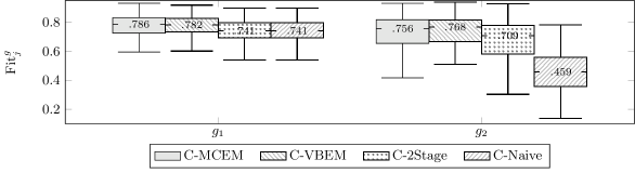
Figure 4: Results of the estimation of cascaded linear systems.

From the figure, it appears that the proposed approximation methods are able to reconstruct the cascaded model with higher accuracy than the alternative approaches we have considered. Furthermore, there seems to be no clear disadvantage in using the variational Bayes approximation as compared to the, more correct, sampling-based approximation. Regarding the performance of the methods in estimating $g_{1}$, we see that the methods C-MCEM and C-VBEM perform better than the other methods (which give the same result). Both C-2Stage and C-Naive only use the information in $v$ to estimate $g_{1}$, whereas C-MCEM and C-VBEM use the full joint distribution of $v$ and $y$ to estimate $g_{1}$. Given that in our setting the noise on $y$ is much lower than the noise on $v$, there is information in $y$ that the joint methods are able to leverage to improve the estimate of $g_{1}$ (similar phenomena were already observed in [21], and in [16]). This allows C-MCEM and C-VBEM to better estimate $g_{1}$.

7.2 Hammerstein systems

In this numerical experiment, we estimate Hammerstein systems with the structure presented in Section 3.5. We perform four Monte Carlo experiments consisting of 500 runs. In each run, we generate a stable transfer-function model by sampling poles and zeros in the complex plane. We sample the poles, uniformly in magnitude and phase, in the annulus of radii 0.4 and 0.8. We sample the zeros uniformly in the disk of radius 0.92. We generate the nonlinear transformation as a finite combination of Legendre polynomials defined as

$$\varphi_{j}(x)=2^{j}\cdot\sum_{k=0}^{j}x^{k}\binom{j}{x}\binom{\tfrac{j+k-1}{2}}{j}.$$ (87)

We sample the coefficients of the combination independently and uniformly in the interval $\mathinner{\left[-1,1\right]}$.

In each Monte Carlo experiment, we consider Hammerstein systems with different orders for both the nonlinear system and the polynomial nonlinearity. In Table 1, we present the orders of the systems considered in the various experiments.

Table 1: Orders of the Hammerstein systems used in the simulations.

Dataset	$S$	$f(\cdot)$
LOLO (Low-Low)	$\{3,\ldots,5\}$	$\{5,\ldots,10\}$
HILO (High-Low)	$\{9,\ldots,20\}$	$\{5,\ldots,10\}$
LOHI (Low-High)	$\{3,\ldots,5\}$	$\{15,\ldots,20\}$
HIHI (High-High)	$\{9,\ldots,20\}$	$\{15,\ldots,20\}$

We simulate the responses of the systems in the datasets to a uniform white noise input in the interval $\mathinner{\left[-1,1\right]}$. We collect $N=200$ samples of the output, from zero initial conditions, and we estimate the static nonlinearity and the impulse response.

As described in Section 3.5, the linear blocks are modeled as zero-mean Gaussian processes with first order stable-spline kernels. We consider both a parametric model and a nonparametric model for the static nonlinearity. All the methods are initialized with $\rho_{1}=1$, $\rho_{2}=0.6$. The noise variances are initialized from the prediction error of an overparameterized least-squares estimate (see [3, 40]).

In the simulation, we compare the performance of the following estimators:

H-P

A semiparametric model for the Hammerstein system. It uses the Legendre polynomial basis to construct a linear parameterization (with the correct order) of the input:

$$\mu_{w}(\theta)=\Phi\theta,\qquad\mathinner{\bigl{[}\Phi\bigr{]}}_{i,j}=\varphi_{j}(u_{i}).$$ (88)

The dynamical system is modeled as a zero-mean Gaussian process with covariance matrix given by the first order stable-spline kernel.

H-MCEM

A nonparametric model for the Hammerstein system with Gibbs sampling from the joint posterior with $B=200$ and $M=500$. It uses the radial-basis-function kernel (27) to model the input nonlinearity. Note that, because the Hammerstein system is not identifiable, we fix $\theta_{1}=1$ in the algorithm.

H-VBEM

A nonparametric model for the Hammerstein system with variational-Bayes approximation of the joint posterior. It uses the same kernel as H-MCEM to model the input nonlinearity.

NLHW

The parametric model in Matlab with the default parameters. It corresponds to the maximum-likelihood estimator of the model with the correct parameterization.

In all methods, the EM iterations are stopped once the relative change in the parameter values is below $10^{-2}$.

To evaluate the performance of the methods, we use the standard goodness-of-fit criterion (86) for the impulse response of the linear system. For the input nonlinearity, we compute the estimated value $\hat{w}_{j}$ on a uniform grid of 300 values between -1 and 1 and we compare it to the true value $w_{j}$ according to

$$\mathrm{Fit}^{f}_{j}=1-\frac{\mathinner{\!\left\lVert w_{j}-\hat{w}_{j}\right\rVert}}{\mathinner{\!\left\lVert w_{j}-\mathrm{mean}(w_{j})\right\rVert}},$$ (89)

where $w_{j}$ is the vector of values of the true nonlinearity ot the $j$th Monte Carlo run, and $\hat{w}_{j}$ is an estimate of the same vector of values.

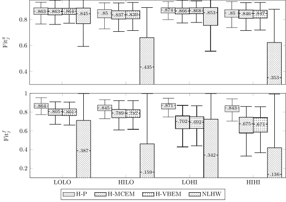
Figure 5: Boxplot of the estimation result

The result of the experiment are presented in Figure 5. The figure shows the boxplots of the fit of the estimated impulse responses (upper pane) and of the static nonlinearities (lower pane) over the systems in the datasets.

From this simulation, it appears that the proposed nonparametric models are capable of recovering the system better than the fully parametric NLHW. In addition, it appears that using the correct parametric model for the input nonlinearity is beneficial in terms of accuracy. As was the case in the cascaded-system estimation problem, the two approximation methods have comparable performance.

8 Conclusions

In this work, we have proposed a new model structure, which we have called the uncertain-input model. Uncertain-input models describe linear systems subject to inputs about which we have limited information. To encode the information we have available about the input and the system, we have used Gaussian-process models.

We have shown how classical problems in system identification can be seen as uncertain-input estimation problems. Among these applications we find classical PEM, errors-in-variables and blind system-identification problems, identification of cascaded linear systems, and identification of Hammerstein models.

We have proposed an iterative algorithm to estimate the uncertain-input model. We estimate the impulse response of the linear system and the input nonlinearity as the posterior means of the Gaussian-process models given the data. The hyperparameters of the Gaussian-process models are estimated using the marginal-likelihood method. To solve the related optimization problem, we have proposed an iterative method based on the EM method.

In the general formulation, the model depends on the convolution of two Gaussian processes. Therefore, the joint distribution of the data is not available in closed form. To circumvent this issue, we have proposed specialized models, namely the semiparametric and the parametric models, for which the integrals defining the posterior distributions are available. In the more general case, we have proposed two approximation methods for the joint posterior distribution. In the first method, we have used a particle approximation of the posterior distribution. The particles are drawn using the Gibbs sampler from Gaussian full-conditional distributions. In the second method, we have used the variational-Bayes approach to approximate the posterior distribution. Using a mean-field approximation, we have found that the posterior distribution can be approximated as a product of two independent Gaussian random variables.

We have tested the proposed model on two problems: the estimation of cascaded linear systems and of Hammerstein models. In both cases, the proposed uncertain-input formulation is able to capture the systems and to provide good estimates.

Although hinged on the EM method (which is guaranteed to converge under certain smoothness assumptions) the approximate methods we have proposed do not have general convergence guarantees: in the formulation given by (12), there may instances of uncertain-input models for which the assumptions required for convergence may not hold. In future publications, we plan to analyze whether there exists general conditions on the uncertain-input model such that the algorithms are guaranteed to converge to optimal solutions.

In addition, the uncertain-input model can be nonidentifiable in certain configurations (for instance, consider the general errors-in-variables problem). We plan to further explore this nonidentifiability. Connections with other problems sharing the same bilinear structure [5, 48] outside of the system identification framework are also under investigation.

Appendix A Proofs of the main results

A.1 Proof of Theorem 1

We consider the complete-data likelihood $\mathrm{p}(y,w,g;\tau)$ where $g$ acts as latent variables. We have that

$$\mathrm{p}(y,v,g;\tau) =\int\mathrm{p}(y,v,g,w;\tau)\operatorname{d\!}w=\int\mathrm{p}(y|g,w;\sigma_{y}^{2})\mathrm{p}(v|w;\sigma_{v}^{2})\mathrm{p}(g;\rho)\mathrm{p}(w;\theta)\operatorname{d\!}w$$ (90)

$$=\mathrm{p}(y|g,w=\mu_{w}(\theta);\sigma_{y}^{2})\mathrm{p}(v|w=\mu_{w}(\theta);\sigma_{v}^{2})\mathrm{p}(g;\rho),$$

where we have used the sampling property of the Dirac density. Hence,

$$\log\mathrm{p}(y,v,g;\tau) =-\frac{1}{2\sigma_{y}^{2}}\mathinner{\!\left\lVert y-G\mu_{w}\right\rVert}^{2}-\frac{N}{2}\log\sigma_{y}^{2}-\frac{1}{2\sigma_{v}^{2}}\mathinner{\!\left\lVert v-\mu_{w}\right\rVert}^{2}-\frac{N}{2}\log\sigma_{v}^{2}$$ (91)

$$-\frac{1}{2}\mathinner{\!\left\lVert g-\mu_{g}\right\rVert}_{{K_{g}}^{-1}}^{2}-\frac{1}{2}\log\det K_{g}\,,$$

where we have dropped explicit dependencies on the hyperparameters. Taking expectations with respect to $\mathrm{p}(g|y,v;\hat{\theta}^{(k)})$, we have that $\mathbf{E}\mathinner{\bigl{\{}\mathinner{\!\left\lVert y-G\mu_{w}\right\rVert}^{2}\!\bigr{\}}}\!=\!y^{T}y-2y^{T}\mathbf{E}\mathinner{\left\{G\right\}}\mu_{w}+\mu_{w}^{T}\mathbf{E}\mathinner{\bigl{\{}G^{T}G\bigr{\}}}\mu_{w}$. The matrix $R$ in (42) is such that $G^{T}=R(I_{N}\otimes g)$; hence, we have that

$$\mathbf{E}\{G^{T}\} =\mathbf{E}\{R(I_{N}\otimes g)\}=R(I_{N}\otimes\hat{g}^{(k)})=\hat{G}^{(k)T},$$ (92)

$$\mathbf{E}\mathinner{\bigl{\{}G^{T}G\bigr{\}}} =\mathbf{E}\mathinner{\left\{R(I_{N}\otimes g)(I_{N}\otimes g^{T})R\right\}}=R(I_{N}\otimes\mathbf{E}\{gg^{T}\})R^{T}=R(I_{N}\otimes\hat{P}_{g}^{(k)}+\hat{g}^{(k)}\hat{g}^{(k)T})R^{T}$$

$$=R(I_{N}\otimes\hat{P}_{g}^{(k)})R+R(I_{N}\otimes\hat{g}^{(k)}\hat{g}^{(k)T})R^{T}=\hat{S}_{g}^{(k)}+R(I_{N}\otimes\hat{g}^{(k)})(I_{N}\otimes\hat{g}^{(k)T})R^{T}$$

$$=\hat{S}_{g}^{(k)}+\hat{G}^{(k)T}\hat{G}^{(k)};$$

hence, $\mathbf{E}\mathinner{\bigl{\{}\mathinner{\!\left\lVert y-G\mu_{w}\right\rVert}^{2}\!\bigr{\}}}\!=\!\mathinner{\!\bigl{\lVert}y-\hat{G}^{(k)}\mu_{w}\bigr{\rVert}}^{2}+\mathinner{\!\left\lVert\mu_{w}\right\rVert}^{2}_{\hat{S}_{g}^{(k)}}$.

Similarly,

$$\mathbf{E} \mathinner{\left\{\mathinner{\!\left\lVert g-\mu_{g}\right\rVert}^{2}\!\right\}}\!\!=\!\operatorname{\mathrm{Tr}\!}\mathinner{\Bigl{\{}K_{g}^{-1}\!\!\mathinner{\left[\mathbf{E}\{gg^{T}\}\!-\!2\mu_{g}\mathbf{E}\{g^{T}\}\!+\!\mu_{g}\mu_{g}^{T}\right]}\!\Bigr{\}}}$$ (93)

$$=\operatorname{\mathrm{Tr}\!}\mathinner{\Bigl{\{}K_{g}^{-1}\mathinner{\left[\hat{P}_{g}^{(k)}+\hat{g}^{(k)}g^{(k)T}-2\mu_{g}\hat{g}^{(k)T}+\mu_{g}\mu_{g}^{T}\right]}\Bigr{\}}}$$

$$=\mathinner{\!\left\lVert\hat{g}^{(k)}-\mu_{g}\right\rVert}^{2}_{K_{g}^{-1}}+\operatorname{\mathrm{Tr}\!}\mathinner{\Bigl{\{}K_{g}^{-1}\hat{P}_{g}^{(k)}\Bigr{\}}}.$$

Plugging these expressions into the expectation of (91) we find (44).

A.2 Proof of Theorem 2

Let $\bar{g}^{(j)}$ and $\bar{w}^{(j)}$ be samples draw from the stationary distribution of the Gibbs sampler with hyperparameters $\hat{\tau}$. Now, consider the complete-data likelihood

$$\log\mathrm{p}(y,v|w,g;\tau)\mathrm{p}(g;\rho)\mathrm{p}(w;\theta)=-\frac{1}{2\sigma_{v}^{2}}\mathinner{\!\left\lVert v-w\right\rVert}^{2}-\frac{N}{2}\log\sigma_{v}^{2}-\frac{1}{2\sigma_{y}^{2}}\mathinner{\!\left\lVert y-Wg\right\rVert}^{2}-\frac{N}{2}\log\sigma_{y}^{2}$$ (94)

$$\quad-\frac{1}{2}\mathinner{\!\left\lVert g-\mu_{g}\right\rVert}_{K_{g}}^{2}-\frac{1}{2}\log\det K_{g}-\frac{1}{2}\mathinner{\!\left\lVert w-\mu_{w}\right\rVert}_{K_{w}}^{2}-\frac{1}{2}\log\det K_{w}\,,$$

where we have dropped the explicit dependencies on the hyperparameters. We have that

$$Q^{\text{{mc}}}(\tau,\hat{\tau})\mathrel{\mathop{\mathchar 58\relax}}=-\frac{1}{2M\sigma_{v}^{2}}\sum_{j=1}^{M}\mathinner{\!\left\lVert v-\bar{w}^{(j)}\right\rVert}^{2}-\frac{N}{2}\log\sigma_{v}^{2}-\frac{1}{2M\sigma_{y}^{2}}\sum_{j=1}^{M}\mathinner{\!\left\lVert y-\bar{W}^{(j)}\bar{g}^{(j)}\right\rVert}^{2}-\frac{N}{2}\log\sigma_{y}^{2}$$ (95)

$$\quad-\frac{1}{2M}\sum_{j=1}^{M}\mathinner{\!\left\lVert\bar{g}^{(j)}-\mu_{g}\right\rVert}_{{K_{g}}^{-1}}^{2}-\frac{1}{2}\log\det K_{g}-\frac{1}{2M}\sum_{j=1}^{M}\mathinner{\!\left\lVert\bar{w}^{(j)}-\mu_{w}\right\rVert}_{{K_{w}}^{-1}}^{2}-\frac{1}{2}\log\det K_{w}\,.$$

Using the definitions in (60), we have that

$$\sum_{j=1}^{M} \mathinner{\!\bigl{\lVert}\bar{g}^{(j)}\!-\!\mu_{g}\bigr{\rVert}}^{2}_{{K_{g}}^{-1}}\!=\!\sum_{j=1}^{M}\operatorname{\mathrm{Tr}\!}\mathinner{\left\{K_{g}^{-1}(\bar{g}^{(j)}\!-\!\mu_{g}){(\bar{g}^{(j)}\!\!-\!\mu_{g})}^{T}\right\}}$$ (96)

$$=\sum_{j=1}^{M}\operatorname{\mathrm{Tr}\!}\mathinner{\left\{K_{g}^{-1}(\bar{g}^{(j)}\!-\!\hat{g}\!+\!\hat{g}\!-\!\mu_{g}){(\bar{g}^{(j)}\!-\!\hat{g}\!+\!\hat{g}\!-\!\mu_{g})}^{T}\right\}}$$

$$=\sum_{j=1}^{M}\operatorname{\mathrm{Tr}\!}\mathinner{\left\{K_{g}^{-1}(\bar{g}^{(j)}\!-\!\hat{g})(\bar{g}^{(j)}\!-\!\hat{g})\right\}}+M\mathinner{\!\left\lVert\hat{g}\!-\!\mu_{g}\right\rVert}_{K_{g}^{-1}}^{2}$$

$$=\operatorname{\mathrm{Tr}\!}\mathinner{\left\{K_{g}^{-1}\sum_{j=1}^{M}(\bar{g}^{(j)}\!-\!\hat{g})(\bar{g}^{(j)}\!-\!\hat{g})\right\}}+M\mathinner{\!\left\lVert\hat{g}\!-\!\mu_{g}\right\rVert}_{K_{g}^{-1}}^{2}$$

$$=M\operatorname{\mathrm{Tr}\!}\mathinner{\left\{K_{g}^{-1}\hat{P}_{g}\right\}}+M\mathinner{\!\left\lVert\hat{g}\!-\!\mu_{g}\right\rVert}_{K_{g}^{-1}}^{2};$$

similarly,

$$\sum_{j=1}^{M}\mathinner{\!\bigl{\lVert}\bar{w}^{(j)}\!-\!\mu_{w}\bigr{\rVert}}^{2}_{{K_{w}}^{-1}}\!=\!M\operatorname{\mathrm{Tr}\!}\mathinner{\left\{K_{w}^{-2}\hat{P}_{w}\right\}}+M\mathinner{\!\left\lVert\hat{w}\!-\!\mu_{w}\right\rVert}_{K_{w}^{-1}}^{2};$$ (97)

Plugging these expressions into (95) we obtain (60).

A.3 Proof of Theorem 3

Consider the complete-data likelihood (94). From (76) we have that $\log\mathrm{q}_{w}^{\star}=\mathbf{E}\mathinner{\left\{\log p(y,v,g,w;\tau)\right\}}$, where the expectation is taken with respect to $\mathrm{q}_{g}^{\star}$. Then, disregarding terms independent of $w$, we have that

$$\log\mathrm{q}_{w}^{\star}\cong\mathbf{E}\mathinner{\left\{-\frac{\mathinner{\!\left\lVert y-Gw\right\rVert}^{2}}{2\sigma_{y}^{2}}-\frac{\mathinner{\!\left\lVert v-w\right\rVert}^{2}}{2\sigma_{v}^{2}}-\mathinner{\!\left\lVert w-\mu_{w}\right\rVert}_{{K_{w}}^{-1}}^{2}\right\}}\cong-\frac{1}{2}\mathinner{\!\left\lVert w\right\rVert}_{P_{w}^{-1}}^{2}+w^{T}m_{w},$$ (98)

where

$$P_{w}=\mathinner{\left(\frac{1}{\sigma_{y}^{2}}\mathbf{E}\{G^{T}G\}+\frac{1}{\sigma_{v}^{2}}I_{n}+K_{w}^{-1}\right)}^{-1},\qquad m_{w}=P_{w}\mathinner{\left(\frac{1}{\sigma_{y}^{2}}\mathbf{E}\{G^{T}\}y+\frac{1}{\sigma_{v}^{2}}v+K_{w}^{-1}\mu_{w}\right)}.$$ (99)

Because it is quadratic in $w$, $\mathrm{q}_{w}$ is a Gaussian distribution. Similarly,

$$\log\mathrm{q}_{g}^{\star}\cong\mathbf{E}\mathinner{\left\{-\frac{\mathinner{\!\left\lVert y-Wg\right\rVert}^{2}}{2\sigma_{y}^{2}}-\mathinner{\!\left\lVert g-\mu_{g}\right\rVert}_{{K_{g}}^{-1}}^{2}\right\}}\cong-\frac{1}{2}\mathinner{\!\left\lVert g\right\rVert}_{P_{g}^{-1}}^{2}+g^{T}m_{g},$$ (100)

where

$$P_{g}=\mathinner{\left(\frac{1}{\sigma_{y}^{2}}\mathbf{E}\{W^{T}W\}+K_{g}^{-1}\right)}^{-1},\qquad m_{g}=P_{g}\mathinner{\left(\frac{1}{\sigma_{y}^{2}}\mathbf{E}\{W^{T}\}y+K_{g}^{-1}\mu_{g}\right)}.$$ (101)

and where all expectations are taken with respect to $\mathrm{q}^{\star}_{w}$. Because it is quadratic in $g$, $\mathrm{q}_{g}$ is also a Gaussian distribution.

A.4 Proof of Corollary 3

Tracing the proof of Theorem 3, we have that $\mathrm{q}_{w}^{(j+1)}$ is a Gaussian distribution with covariance matrix and mean given by (99) where the expectations are taken with respect to $\mathrm{q}_{g}^{(j)}$. Using the matrix $R$ in (42), we have

$$\mathbf{E}\{G^{T}G\} =\mathbf{E}\{R(I_{N}\otimes g)(I_{N}\otimes g^{T})R^{T}\}=R(I_{N}\otimes\mathbf{E}\{gg^{T}\})R^{T}=T_{g}^{(j)},$$ (102)

$$\mathbf{E}\{G^{T}\} =\mathbf{E}\{R(I_{N}\otimes g)\}=R(I_{N}\otimes g^{(j+1)})=G^{(j)T}.$$

Similarly, $\mathrm{q}_{g}^{(j+1)}$ is a Gaussian distribution with covariance matrix and mean given by (101), where the expectations are taken with respect to $\mathrm{q}_{w}^{(j+1)}$. We have that

$$\mathbf{E}\{W^{T}W\} =\mathbf{E}\{R(I_{N}\otimes w)(I_{N}\otimes w^{T})R^{T}\}=R(I_{N}\otimes\mathbf{E}\{ww^{T}\})R^{T}=T_{w}^{(j+1)},$$ (103)

$$\mathbf{E}\{W^{T}\} =R(I_{N}\otimes w^{(j+1)})=W^{(j+1)T}.$$

Plugging these expectations into (101) and (99) we obtain (80).

A.5 Proof of Theorem 4

We consider again the complete-data likelihood (94). Taking the expectation with respect to the independent Gaussian densities $\mathrm{q}_{g}^{(k)}$ and $\mathrm{q}_{w}^{(k)}$, we have that

$$\mathbf{E}\mathinner{\left\{\mathinner{\!\left\lVert v-w\right\rVert}^{2}\right\}}=\hat{R}_{v}^{(k)}+\operatorname{\mathrm{Tr}\!}\,\{\hat{P}^{(k)}\},$$ (104)

$$\mathbf{E}\mathinner{\left\{\mathinner{\!\left\lVert g-\mu_{g}\right\rVert}_{{K_{g}}^{-1}}^{2}\right\}}=\mathinner{\!\bigl{\lVert}\hat{g}^{(k)}-\mu_{g}\bigr{\rVert}}^{2}_{{K_{g}}^{-1}}+\operatorname{\mathrm{Tr}\!}\,\{K_{g}^{-1}\hat{P}_{g}^{(k)}\},$$ (105)

$$\mathbf{E}\mathinner{\left\{\mathinner{\!\left\lVert w-\mu_{w}\right\rVert}_{{K_{w}}^{-1}}^{2}\right\}}=\mathinner{\!\bigl{\lVert}\hat{w}^{(k)}-\mu_{w}\bigr{\rVert}}^{2}_{{K_{w}}^{-1}}+\operatorname{\mathrm{Tr}\!}\,\{K_{w}^{-1}\hat{P}_{w}^{(k)}\}.$$ (106)

Note that $\mathbf{E}\{W^{T}W\}=R^{T}(I_{N}\otimes\hat{P}_{w}^{(k)}+\hat{w}^{(k)}\hat{w}^{(k)T})R=R^{T}(I_{N}\otimes\hat{P}_{w}^{(k)})R+R^{T}(I_{N}\otimes\hat{w}^{(k)}\hat{w}^{(k)T})R=\hat{S}_{w}^{(k)}+\hat{W}^{(k)T}\hat{W}^{(k)}=\hat{T}_{w}^{(k)}$, and that $\mathbf{E}\{g^{T}W^{T}Wg\}=\operatorname{\mathrm{Tr}\!}\{\hat{T}_{w}^{(k)}(P_{g}^{(k)}+\hat{g}^{(k)}\hat{g}^{(k)T})=\mathinner{\!\bigl{\lVert}\hat{W}^{(k)}\hat{g}^{(k)}\bigr{\rVert}}^{2}+\mathinner{\!\bigl{\lVert}\hat{g}^{(k)}\bigr{\rVert}}_{S_{w}^{(k)}}^{2}+\operatorname{\mathrm{Tr}\!}\{\hat{T}_{w}^{(k)}\hat{P}_{g}^{(k)}\}$, Hence, $\mathbf{E}\mathinner{\left\{\mathinner{\!\left\lVert y-Wg\right\rVert}^{2}\right\}}=y^{T}y-2y^{T}\mathbf{E}\{Wg\}+\mathbf{E}\{g^{T}W^{T}Wg\}=\hat{R}y^{(k)}+\mathinner{\!\bigl{\lVert}\hat{g}^{(k)}\bigr{\rVert}}_{S_{w}^{(k)}}^{2}+\operatorname{\mathrm{Tr}\!}\,\{\hat{T}_{w}^{(k)}\hat{P}_{g}^{(k)}\}$. Plugging the terms in the expression of the complete likelihood, we get (83).

Appendix B Acknowledgment

This work was supported by the Swedish Research Council via the projects NewLEADS (contract number: 2016-06079) and System identification: Unleashing the algorithms (contract number: 2015-05285), and by the European Research Council under the advanced grant LEARN (contract number: 267381).

References

• [1] K. Abed-Meraim, W. Qiu, and Y. Hua. Blind system identification. Proc. IEEE, 85(8):1310–1322, 1997.
• [2] A. Ahmed, B. Recht, and J. Romberg. Blind deconvolution using convex programming. IEEE Trans. Inform. Theory, 60(3):1711–1732, 2014.
• [3] E. W. Bai. An optimal two-stage identification algorithm for Hammerstein–Wiener nonlinear systems. Automatica, 34(3):333–338, 1998.
• [4] E. W. Bai and D. Li. Convergence of the iterative Hammerstein system identification algorithm. IEEE Trans. Autom. Control, 49(11):1929–1940, 2004.
• [5] E. W. Bai and Y. Liu. On the least squares solutions of a system of bilinear equations. In Proc. IEEE Conf. Decis. Control (CDC). IEEE, 2005.
• [6] M. J. Beal. Variational Algorithms for Approximate Bayesian Inference. PhD thesis, Gatsby Computational Neuroscience Unit, University College London, 2003.
• [7] J. O. Berger, B. Liseo, and R. L. Wolpert. Integrated likelihood methods for eliminating nuisance parameters. Statist. Sci., 14(1):1–28, 1999.
• [8] J. M. Bernardo and A. F. M. Smith. Bayesian Theory. JOHN WILEY & SONS INC, 2000.
• [9] C. M. Bishop. Pattern Recognition and Machine Learning. Springer, 2006.
• [10] G. Bottegal, R. S. Risuleo, and H. Hjalmarsson. Blind system identification using kernel-based methods. In Proc. IFAC Symp. System Identification (SYSID), volume 48, pages 466–471, 2015.
• [11] S. Boyd and L. Vandenberghe. Convex Optimization. Cambridge University Press, 2004.
• [12] P. Castaldi and U. Soverini. Identification of dynamic errors-in-variables models. Automatica, 32(4):631–636, 1996.
• [13] T. Chen and L. Ljung. Constructive state space model induced kernels for regularized system identification. In Proc. IFAC World Cong., volume 19, pages 1047–1052, 2014.
• [14] A. P. Dempster, N. M. Laird, and D. B. Rubin. Maximum likelihood from incomplete data via the em algorithm. J. R. Stat. Soc. Ser. B. Stat. Methodol., pages 1–38, 1977.
• [15] F. Dinuzzo. Kernels for linear time invariant system identification. SIAM J. Control Optim., 53(5):3299–3317, 2015.
• [16] N. Everitt, C. Rojas, and H. Hjalmarsson. A geometric approach to variance analysis of cascaded systems. In Proc. IEEE Conf. Decis. Control (CDC), 2013.
• [17] R. Frigola, F. Lindsten, T. B. Schön, and C. E. Rasmussen. Identification of gaussian process state-space models with particle stochastic approximation EM. IFAC Proc. Vol., 47(3):4097–4102, 2014.
• [18] S. Geman and D. Geman. Stochastic relaxation, Gibbs distributions, and the Bayesian restoration of images. IEEE Trans. Pattern Anal. Mach. Intell., (6):721–741, 1984.
• [19] W. R. Gilks, S. Richardson, and D. J. Spiegelhalter. Markov Chain Monte Carlo in Practice. Chapman and Hall London, 1996.
• [20] F. Giri and E. W. Bai. Block-oriented nonlinear system identification. Springer, 2010.
• [21] H. Hjalmarsson. System identification of complex and structured systems. Eur. J. Control, 15(3-4):275–310, 2009.
• [22] S. Kullback and R. A. Leibler. On information and sufficiency. Ann. Math. Statist., 22(1):79–86, 1951.
• [23] J. Linder and M. Enqvist. Identification of systems with unknown inputs using indirect input measurements. International Journal of Control, 90(4):729–745, 2017.
• [24] L. Ljung. System Identification, Theory for the User. Prentice Hall, 1999.
• [25] J. Maritz and T. Lwin. Empirical bayes methods. Chapman and Hall London, 1989.
• [26] I. Markovsky and K. Usevich. Structured low-rank approximation with missing data. SIAM J. Matrix Anal. & Appl., 34(2):814–830, 2013.
• [27] D. B. McCombie, A. T. Reisner, and H. H. Asada. Laguerre-model blind system identification: Cardiovascular dynamics estimated from multiple peripheral circulatory signals. IEEE Trans. Biomed. Eng., 52(11):1889–1901, 2005.
• [28] G. McLachlan and T. Krishnan. The EM algorithm and extensions, volume 382. John Wiley and Sons, 2007.
• [29] X. L. Meng and D. B. Rubin. Maximum likelihood estimation via the ECM algorithm: A general framework. Biometrika, 80(2):267–278, 1993.
• [30] E. Moulines, P. Duhamel, J. F. Cardoso, and S. Mayrargue. Subspace methods for the blind identification of multichannel FIR filters. IEEE Trans. Signal Process., 43(2):516–525, 1995.
• [31] N. Nakajima. Blind deconvolution using the maximum likelihood estimation and the iterative algorithm. Opt. Commun., 100(1-4):59–66, 1993.
• [32] R. C. Neath. On convergence properties of the Monte Carlo EM algorithm. In Advances in Modern Statistical Theory and Applications: A Festschrift in honor of Morris L. Eaton, pages 43–62. Institute of Mathematical Statistics, 2013.
• [33] H. Ohlsson, L. J. Ratliff, R. Dong, and S. S. Sastry. Blind identification via lifting. In Proc. IFAC World Cong., 2014.
• [34] G. Pillonetto and A. Chiuso. A Bayesian learning approach to linear system identification with missing data. In Proc. IEEE Conf. Decis. Control (CDC), pages 4698–4703, 2009.
• [35] G. Pillonetto, F. Dinuzzo, T. Chen, G. De Nicolao, and L. Ljung. Kernel methods in system identification, machine learning and function estimation: A survey. Automatica, 50(3):657–682, 2014.
• [36] G. Pillonetto, M. H. Quang, and A. Chiuso. A new kernel-based approach for nonlinear system identification. IEEE Trans. Autom. Control, 56(12):2825–2840, 2011.
• [37] Gianluigi Pillonetto and Giuseppe De Nicolao. A new kernel-based approach for linear system identification. Automatica, 46(1):81–93, 2010.
• [38] C. Rasmussen and C. Williams. Gaussian processes for machine learning. the MIT Press, 2006.
• [39] R. S. Risuleo, G. Bottegal, and H. Hjalmarsson. A kernel-based approach to Hammerstein system identication. In Proc. IFAC Symp. System Identification (SYSID), volume 48, pages 1011–1016, 2015.
• [40] R. S. Risuleo, G. Bottegal, and H. Hjalmarsson. A new kernel-based approach to overparameterized Hammerstein system identification. In Proc. IEEE Conf. Decis. Control (CDC), pages 115–120, 2015.
• [41] R. S. Risuleo, G. Bottegal, and H. Hjalmarsson. On the estimation of initial conditions in kernel-based system identification. In Proc. IEEE Conf. Decis. Control (CDC), pages 1120–1125, 2015.
• [42] R. S. Risuleo, G. Bottegal, and H. Hjalmarsson. Kernel-based system identification from noisy and incomplete input-output data. In Proc. IEEE Conf. Decis. Control (CDC). Institute of Electrical and Electronics Engineers (IEEE), 2016.
• [43] T. Söderström. Why are errors-in-variables problems often tricky? In Proc. European Control Conf. (ECC), pages 802–807, 2003.
• [44] T. Söderström. Errors-in-variables methods in system identification. Automatica, 43(6):939–958, 2007.
• [45] T. Söderström. System identification for the errors-in-variables problem. In Proc. UKACC Int. Conf. Control, pages 1–14, 2010.
• [46] A. Svensson and T. B. Schön. A flexible state–space model for learning nonlinear dynamical systems. Automatica, 80:189–199, 2017.
• [47] R. Wallin and A. Hansson. Maximum likelihood estimation of linear SISO models subject to missing output data and missing input data. Int. J. Control, pages 1–11, 2014.
• [48] J. Wang, Q. Zhang, and L. Ljung. Revisiting the two-stage algorithm for hammerstein system identification. In Proc. IEEE Conf. Decis. Control (CDC). IEEE, 2009.
• [49] G. C. G. Wei and M. A. Tanner. A Monte Carlo implementation of the EM algorithm and the poor man’s data augmentation algorithms. Journal of the American Statistical Association, 85(411):699–704, 1990.
• [50] C. F. J. Wu. On the convergence properties of the EM algorithm. Ann. Statist., 11(1):95–103, 1983.
• [51] E. Zhang and R. Pintelon. Errors-in-variables identification of dynamic systems in general cases. In Proc. IFAC Symp. System Identification (SYSID), volume 48, pages 309–313, 2015.