Clustering dark energy and halo abundances

Abstract

Within the standard paradigm, dark energy is taken as a homogeneous fluid that drives the accelerated expansion of the universe and does not contribute to the mass of collapsed objects such as galaxies and galaxy clusters. The abundance of galaxy clusters – measured through a variety of channels – has been extensively used to constrain the normalization of the power spectrum: it is an important probe as it allows us to test if the standard $\Lambda$CDM model can indeed accurately describe the evolution of structures across billions of years. It is then quite significant that the Planck satellite has detected, via the Sunyaev-Zel’dovich effect, less clusters than expected according to the primary CMB anisotropies. One of the simplest generalizations that could reconcile these observations is to consider models in which dark energy is allowed to cluster, i.e., allowing its sound speed to vary. In this case, however, the standard methods to compute the abundance of galaxy clusters need to be adapted to account for the contributions of dark energy. In particular, we examine the case of clustering dark energy – a dark energy fluid with negligible sound speed – with a redshift-dependent equation of state. We carefully study how the halo mass function is modified in this scenario, highlighting corrections that have not been considered before in the literature. We address modifications in the growth function, collapse threshold, virialization densities and also changes in the comoving scale of collapse and mass function normalization. Our results show that clustering dark energy can impact halo abundances at the level of 10%–30%, depending on the halo mass, and that cluster counts are modified by about 30% at a redshift of unity.

1 Introduction

The abundance of galaxy clusters is a powerful tool to study the late time evolution of the universe. These objects are formed at low redshifts and strongly depend on the properties of dark matter, baryons and the physics of cosmic acceleration. Analyses of cluster counts depend crucially on the knowledge of the halo mass function. Thanks to the approximate universality of the mass function, the latter can be calibrated once and for all using large-scale high-resolution $N$-body simulations [1]. However, these computationally very expensive simulations address only the simple standard $\Lambda$CDM model or, at most, a smooth dark energy (DE) with constant equation of state parameter (EoS), $w=\bar{p}_{de}/\bar{\rho}_{de}$. This limits the possible analyses of cluster counts to these very standard models.

Cluster counts have been extensively used to constraint the matter density parameter $\Omega_{m}$ and the normalization $\sigma_{8}$ of the power spectrum, see, e.g., [2, 3, 4, 5]. The abundance of clusters is an important probe in cosmology as it allows us to test the evolution of structures across billions of years. It was then unexpected that the Planck satellite detected via the Sunyaev-Zel’dovich effect less clusters than predicted according to the primary CMB anisotropies [5]. This tension could be due to a poor knowledge of the scaling relation calibration or to a non-standard energy component in the universe. The latter possibility motivates us to extend state-of-the-art mass functions to the case of a dark energy that can cluster and so participate in the formation of collapsed objects such as galaxies and galaxy clusters. The new mass function can then be used to analyze the Planck clusters and see if a clustering dark energy can help in alleviating the tension from Planck [6].

Within General Relativity, the simplest extension with respect to the cosmological constant $\Lambda$ is a dark energy with a time varying equation of state. In this case, DE fluctuations are inevitably present, giving rise to at least a new degree of freedom: the sound speed (in the rest frame of the fluid) $c_{s}=\sqrt{\delta p_{de}/\delta\rho_{de}}$. In quintessence models, DE is represented by a canonical scalar field with a potential, which determines the evolution of the EoS in the range $-1<w\left(t\right)<1$. However, quintessence models always have $c_{s}=1$. This fact implies that quintessence perturbations are very small compared to matter perturbations on small scales (see though [7]). This gives support to the common practice of neglecting DE perturbations in structure formation studies such as $N$-body simulations.

However, there exists many DE models which can be described by a perfect fluid with varying sound speed. Models that show this behavior include the tachyon field [8, 9] and, in general, the whole class of minimally coupled $K$-essence scalar fields [10, 11], in which the sound speed can be freely chosen. Models with negligible sound speed can also be constructed with two scalar fields [12] and effective field theory [13].

When DE has negligible sound speed, its perturbations have no pressure support and can grow at the same pace as matter perturbations. Therefore, they can evolve nonlinearly and impact the formation of galaxy clusters. As cosmological simulations that include DE fluctuations have not yet been conducted, one has to resort to semi-analytical approaches such the spherical collapse model (SCM) [14] together with Press-Schechter (PS) or Sheth-Tormen (ST) mass functions [15, 16] in order to explore the impact of clustering DE in the abundances of halos. In fact, the SCM was generalized to study clustering DE and it was shown that DE fluctuations can indeed become nonlinear, impact matter growth and the critical density threshold for collapse, $\delta_{c}$, and contribute to the mass of the clusters [17, 18, 19, 20, 21, 22, 23, 24, 25]. The impact of clustering DE was also studied in higher order perturbation theory [26, 27, 28].

In this work we carefully examine how the halo mass function is modified in the presence of clustering DE – a dark energy fluid with negligible sound speed – with a redshift-dependent equation of state, highlighting corrections that have not been considered in the literature before. We reanalyze some modifications that were already considered in the literature, such as the growth function, collapse threshold and virialization densities. Moreover, we also consider two new modifications: the comoving scale of collapse and mass function normalization. Section 2 is devoted to the study of the SCM in the case of clustering DE, while Section 3 discusses how the halo mass function is modified in order to take into account the contribution of DE fluctuations to the halo virialization. In Section 4 we show that clustering dark energy can impact halo abundances at the level of 10%–30%, depending on the halo mass, and that cluster counts are modified by about 30% at a redshift of unity. We draw our conclusions in Section 5.

Throughout this work we adopt the following fiducial values of the cosmological parameters: $h=0.7$, $\Omega_{m}=0.3$, $\Omega_{k}=0$, $\Omega_{b}\,h^{2}=0.0223$, $\sigma_{8}=0.8,n_{s}=0.966$.

2 Spherical collapse in the fluid and radius approach

The SC model can be generalized to treat fluids other than pressureless matter using the Pseudo-Newtonian Cosmology approach [19, 20, 21]. This framework is particularly useful to study clustering DE ($c_{s}=0$), in which case the equations are:

$$\dot{\delta}_{m}+3\frac{\theta}{a}\left(1+\delta_{m}\right)=0\,,$$ (2.1)

$$\dot{\delta}_{de}-3wH\delta_{de}+3\frac{\theta}{a}\left(1+w+\delta_{de}\right)=0\,,$$ (2.2)

$$\dot{\theta}+H\theta+\frac{\theta^{2}}{3a}=-4\pi Ga\left(\bar{\rho}_{m}\delta_{m}+\bar{\rho}_{de}\delta_{de}\right)\,,$$ (2.3)

where $\theta$ is the divergence of the peculiar velocity, $\delta_{m}=\delta\rho_{m}/\bar{\rho}_{m}$ and $\delta_{de}=\delta\rho_{de}/\bar{\rho}_{de}$. In this approach, the redshift of collapse, $z_{c}$, is determined when $\delta_{m}\rightarrow\infty$, which is numerically implemented as certain threshold that reproduces the EdS results. As we will show, although this method is widely used to study the nonlinear evolution, the determination of the critical threshold might not be the best approach when DE fluctuations are present.

In order to understand the issue, let us now consider the radial approach. The original SC model, which determines the evolution of a spherical shell of physical radius $R$, only considers pressureless matter and can be solved analytically. When DE with negligible $c_{s}$ is present, the dynamical equation for $R$ can be written as

$$\frac{\ddot{R}}{R}=-\frac{4\pi G}{3}\left[\bar{\rho}_{m}\left(1+\delta_{m}\right)+\bar{\rho}_{de}\left(1+3w+\delta_{de}\right)\right]\,.$$ (2.4)

We also need equations for the contrasts of matter and DE. For matter, we assume that the total mass inside the shell with radius $R$ is conserved, then we have

$$\dot{\delta}_{m}+3\left(\frac{\dot{R}}{R}-\frac{\dot{a}}{a}\right)\left(1+\delta_{m}\right)=0.$$ (2.5)

Comparing with Eq. (2.1), we identify

$$\frac{\theta}{a}=3\left(\frac{\dot{R}}{R}-\frac{\dot{a}}{a}\right).$$ (2.6)

Note that deriving Eq. (2.6) with respect to time and using Eq. (2.4), we recover Eq. (2.3). The radial approach itself can not determine the evolution of DE fluctuations – note that the evolution of matter fluctuations is given by the assumption that the total matter within $R$ is conserved, which is not valid for DE. It is possible to derive an equation for DE fluctuations using the relation between $\theta$ and $R$, and Eq. (2.2), which yields

$$\dot{\delta}_{de}-3wH\delta_{de}+3\left(\frac{\dot{R}}{R}-\frac{\dot{a}}{a}\right)\left(1+w+\delta_{de}\right)=0.$$ (2.7)

Hence, the system of Eqs. (2.4), (2.5) and (2.7) determines the evolution of the shell radius, matter and DE fluctuations. The dynamical evolution in the two approaches is identical, however, as we will show, the commonly used collapse criteria in the two approaches are not equivalent.

In the radius approach, the redshift of collapse, $z_{c}$, is given when $R\rightarrow 0$. In the EdS model, the RHS of Eq. (2.4) only has matter quantities and the critical density of collapse takes the standard value $\delta_{c}=\delta_{m}^{{\rm lin}}\left(z_{c}\right)\simeq 1.686$. In the presence of DE, however, Eq. (2.4) shows that DE fluctuations also contribute to the collapse, hence the density contrast that gives the threshold density contrast has to be modified to take this new contribution into account. Therefore, instead of determining the collapse threshold only with the matter contribution, the natural quantity to use is the weighted total fluctuation:

$$\delta_{{\rm tot}}\left(z\right)=\delta_{m}\left(z\right)+\frac{\Omega_{de}\left(z\right)}{\Omega_{m}\left(z\right)}\delta_{de}\left(z\right).$$ (2.8)

At high-z, when DE is subdominant in the background, the contribution of DE fluctuations to $\delta_{{\rm tot}}$ is very small, regardless of the magnitude of $\delta_{de}$. Conversely, at low-z, DE dominates the background and even relatively small DE fluctuations impact $\delta_{{\rm tot}}$. So, the definition of $\delta_{{\rm tot}}$ reflects the fact the gravitational potential, which drives the evolution of $R$, is sourced by densities fluctuations, $\bar{\rho}\delta$. The same quantify was used to study higher order perturbation theory in clustering quintessence models [26].

The critical contrast is then given by the linearly evolved total fluctuation:

$$\delta_{c}\left(z_{c}\right)=\delta_{{\rm tot}}^{{\rm lin}}\left(z_{c}\right)\,,$$ (2.9)

where $z_{c}$ is the redshift at which $\delta_{{\rm tot}}$ is above a certain numerical threshold. In the same fashion, the normalized growth function is given by

$$G_{{\rm tot}}\left(z\right)=\frac{\delta^{{\rm lin}}_{{\rm tot}}\left(z\right)}{\delta^{{\rm lin}}_{{\rm tot}}\left(0\right)}.$$ (2.10)

Another interesting point about the relation between these two approaches is the error in $\delta_{c}$ when using the fluid approach, as reported in [29] (see also [30]). The authors show that the numerical collapse threshold is not the same for different redshifts, which in turn generates a spurious increase of $\delta_{c}$ with $z$. This can be corrected by calibrating the numerical threshold as a function of the redshift in order to reproduce some known $\delta_{c}$ and demanding that it approaches the EdS value at high-$z$. Once this calibration is done, we verified that both approaches give essentially the same results for the models under consideration in this work. However, the radial approach is more robust because it does not demand any redshift-dependent calibration and for this reason it will be used here.

2.1 Background evolution and growth function

In order to show the impact of DE fluctuations on the halo collapse, we adopt a DE with a linear parametrization of the equation of state, $w=w_{0}+\left(1-a\right)w_{a}$. In this work we do not consider models with $w<-1$ because in such case, during the nonlinear regime, the dynamical evolution can generate $\delta_{de}<-1$, which implies a non-physical negative energy density. In fact, we observed this happens around virialization densities for $1+w\simeq-0.1$. Hence we prefer to focus on the less problematic region of parameter space of non-phantom equations of state in order to clearly show the modifications in the mass function.

The latter happens because in Eq. (2.2) the coupling between the density contrast and gravitational force is proportional to $\left(1+w+\delta_{de}\right)$. Hence, already at the linear regime, matter overdensities will create DE underdensities if $w<-1$. Indeed, in the matter dominated era and for constant $w$ one has [20, 23]:

$$\delta_{de}=\frac{1+w}{1-3w}\delta_{m}\,.$$ (2.11)

In the nonlinear regime, $\delta_{de}$ continues to decrease as $\delta_{m}$ grows, but the coupling does not vanish as $\delta_{de}\rightarrow-1$ negative energy densities can appear. To better understand this behavior, bear in mind that voids of matter always have $\delta_{m}>-1$ because the coupling between its density contrast and gravitational force is $\left(1+\delta_{m}\right)$, so as $\delta_{m}\rightarrow-1$ the coupling vanishes and the decrease in $\delta_{m}$ is halted. In the phantom case, $\left(1+w+\delta_{de}\right)$ is always negative inside matter halos, therefore $\delta_{de}$ continues to decrease as $\delta_{m}$ grows. This pathological behavior might be an indication of a flaw in phantom models with negligible sound speed. This issue is not present for $w>-1$ because in this case matter halos induce positive $\delta_{de}$ and, even in the case of an extreme matter void with $\delta_{m}\simeq-1$, $\delta_{de}$ is smaller in magnitude than $\delta_{m}$ for $w\apprge-1$.

	$w_{0}$	$w_{a}$
S1	-0.9	0.2
S2	-0.9	0.1
S3	-0.9	0
S4	-0.9	-0.1

Table 1: The four sets of parameters $w_{0}$ and $w_{a}$ used in this work.

We choose the four sets of parameters shown in Table 1. As initial conditions, we assume that only the growing mode of matter is present and $\delta_{de}$ is given by Eq. (2.11).

In Figure 1 we show, for each set of parameters, the ratios of the total growth function, $G_{{\rm tot},c_{s}=0}$ (left panel) and the usual matter only growth function, $G_{m,c_{s}=0}$, (right panel) to the matter growth function for the case of negligible DE perturbations, $G_{m,c_{s}=1}$, as a function of redshift. As we can see, the impact of DE perturbations on $G_{{\rm tot}}$ is much larger. Given this fact, we already expect that our proposed growth function will strongly impact the abundance of galaxy clusters. Since all functions are normalized at $z=0$, we can see that clustering DE enhances the growth of perturbations because they grow from smaller values in the past to reach the same value as the homogeneous case today.

Also note that the greatest impact of DE perturbations appear for S1. This happens because S1 has the largest value of $w$ at high-$z$, hence both $\delta_{de}$ and $\Omega_{de}\left(z\right)/\Omega_{m}\left(z\right)$ are enhanced. This kind of behavior is responsible for large deviations of the growth factor with respect to the so called GR value [31].

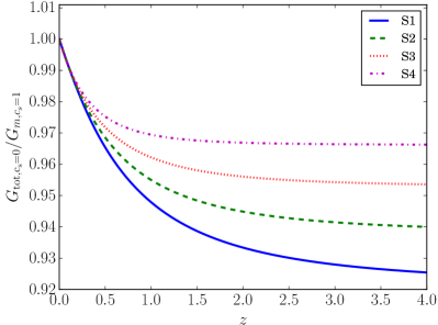
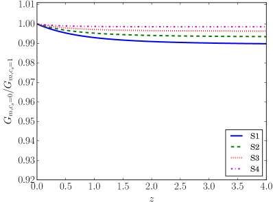
Figure 1: Ratios $G_{{\rm tot},c_{s}=0}/G_{m,c_{s}=1}$ (left panel) and $G_{m,c_{s}=0}/G_{m,c_{s}=1}$ (right panel) as a function of redshift for each set of parameters given in Table 1.

2.2 Virialization

Now we consider the nonlinear evolution of the fluctuations. First we compute the virialization time, which will be used to define the critical density threshold for collapse, the virial mass and virial overdensity.

If $c_{s}=0$, DE fluctuations have no pressure support and follow matter trajectories. Their order of magnitude can be estimated using Eq. (2.11), which also shows that overdensities in matter create overdensities in DE for $w>-1$. Moreover, as DE fluctuations grow in the nonlinear regime, its local equation, $w_{c}=\left(\bar{\rho}+\delta\rho\right)/\left(\bar{p}+\delta p\right)=w\left[1-\delta_{de}/\left(1+\delta_{de}\right)\right]$, tends to zero for $w>-1$, thus indicating that its properties become more similar to matter, see [17, 32].

Therefore, the total mass, $M_{{\rm tot}}$, is expected to have an extra contribution due to DE:

$$M_{{\rm tot}}=M_{m}+M_{{\rm de}}\,.$$ (2.12)

The mass associated with matter is

$$M_{m}=\frac{4\pi}{3}R^{3}\bar{\rho}_{m}\left(z\right)\left[1+\delta_{m}\left(z\right)\right]\,,$$ (2.13)

and is conserved. It is very debatable how to include DE contribution from a phenomenological point of view. Since only DE fluctuations with negligible sound speed are subjected to the same forces that act on matter particles, we define

$$M_{de}=\frac{4\pi}{3}R^{3}\bar{\rho}_{de}\left(z\right)\delta_{de}\left(z\right)\,,$$ (2.14)

which is not conserved throughout the evolution. Note that we are not including the contribution from the homogeneous energy density $\bar{\rho}_{de}$ (that we did include in the case of $M_{m}$). This is choice is also helpful to connect to the case of homogeneous dark energy, whose uniform contribution is not usually taken into account when calculating the halo mass.

In order to determine the virialization time, we use the method described in Ref. [33], which takes into account the non-conservation of $M_{{\rm tot}}$ caused by the inclusion $M_{de}$. In this approach the virialization time is defined when the moment of inertia of a sphere of non-relativistic particles is in steady state, which yields the equation

$$\frac{1}{2M_{{\rm tot}}}\frac{d^{2}M_{{\rm tot}}}{dt^{2}}+\frac{2}{M_{{\rm tot}}R}\frac{dM_{{\rm tot}}}{dt}\frac{dR}{dt}+\frac{1}{R^{2}}\left(\frac{dR}{dt}\right)^{2}+\frac{1}{R}\frac{d^{2}R}{dt^{2}}=0\,.$$ (2.15)

In EdS, $R_{{\rm vir}}=\frac{1}{2}R_{{\rm ta}}$, and $\delta_{m}\left(z_{{\rm v}}\right)\simeq 145.8$, see Ref. [34] for a discussion about this quantity and its impact on the mass function.

In Fig. 2 we show $R_{{\rm v}}/R_{{\rm ta}}$ for each set of parameters and for $c_{s}=0$ and $c_{s}=1$. DE fluctuations affect both the time variation of $M_{\rm tot}$ and $R$. The general modification is that time derivatives of $M_{\rm tot}$ delay the moment of virialization, so $R_{{\rm v}}/R_{{\rm ta}}$ is smaller when DE fluctuations are present.

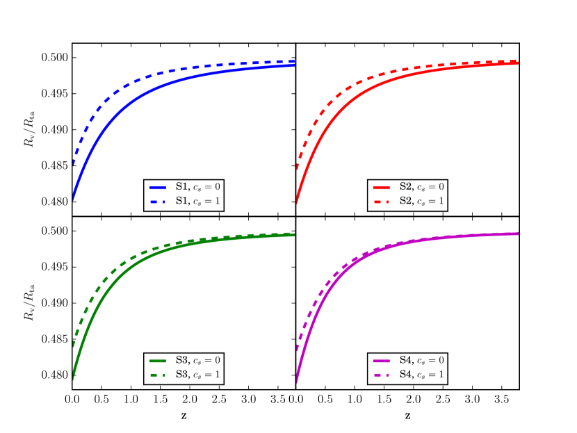
Figure 2: $R_{{\rm v}}/R_{{\rm ta}}$ as a function of the virialization redshift for the set of parameters given in Table 1.

In Fig. 3 (left panel) we show

$$\epsilon\equiv\frac{M_{de}\left(z_{{\rm v}}\right)}{M_{m}\left(z_{\rm{v}}\right)}$$ (2.16)

as a function of virialization redshift. This quantity is important because, as we will show, it is related to the normalization of mass functions and also represents the fraction of DE mass in the halo. It is clear that the contribution of DE increases as DE dominates the background evolution. Since $M_{de}$ gives rise to the non-conservation of total mass, the largest impact of DE fluctuations on quantities computed at virialization is present at very low redshifts. It is important to note that, the larger is $1+w$ at high-$z$, the larger is $\epsilon$. As we can see, DE fluctuations can account for a few % of the total mass of the halo.

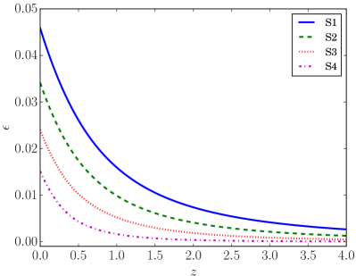
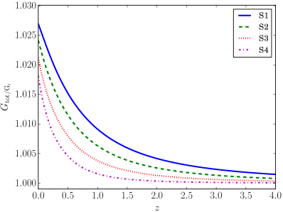
Figure 3: Left Panel: Fraction of DE mass with respect to matter mass, $\epsilon=M_{de}/M_{m}$, as a function of the virialization redshift for the set of parameters given in Table 1. Right Panel: Plot of $G_{\rm tot}/G_{\epsilon}$, see Section 2.2.

As $\epsilon$ gives us the fractional contribution of DE with respect to matter, it should be linked to the contribution of the DE perturbation to $G_{\rm tot}$. It turns out that the function

$$G_{\epsilon}=G_{m,c_{s}=0}\left(1+\epsilon\right)\,,$$ (2.17)

where $G_{m}$ is the matter growth function in the presence of clustering DE, is very similar to $G_{\rm tot}$. As one can see from Fig. 3 (right panel), these two quantities differ at most by $2.6\%$ at very low redshifts. This is a important consistency check between linear and nonlinear quantities that we have defined in this work.

Expressing the total mass of the halo in the form $M_{{\rm tot}}=\frac{4\pi}{3}R_{{\rm vir}}^{3}\bar{\rho}_{c}\Delta_{{\rm v}}$, the virialization overdensity is given by

$$\Delta_{{\rm v}}=\Omega_{m}\left(z_{{\rm v}}\right)\left[1+\delta_{m}\left(z_{{\rm v}}\right)\right]+\Omega_{de}\left(z_{{\rm v}}\right)\delta_{de}\left(z_{{\rm v}}\right)\,.$$ (2.18)

In Fig. 4 we show the evolution of $\Delta_{{\rm v}}$ as a function of redshift for the four different EoS evolution studied. In all cases $\Delta_{{\rm v}}$ becomes smaller at low-$z$, as $\Omega_{m}$ decreases. The presence of DE fluctuations increases $\Delta_{{\rm v}}$, which is a consequence of the delayed virialization that we discussed in the case of $R_{{\rm v}}/R_{{\rm ta}}$.

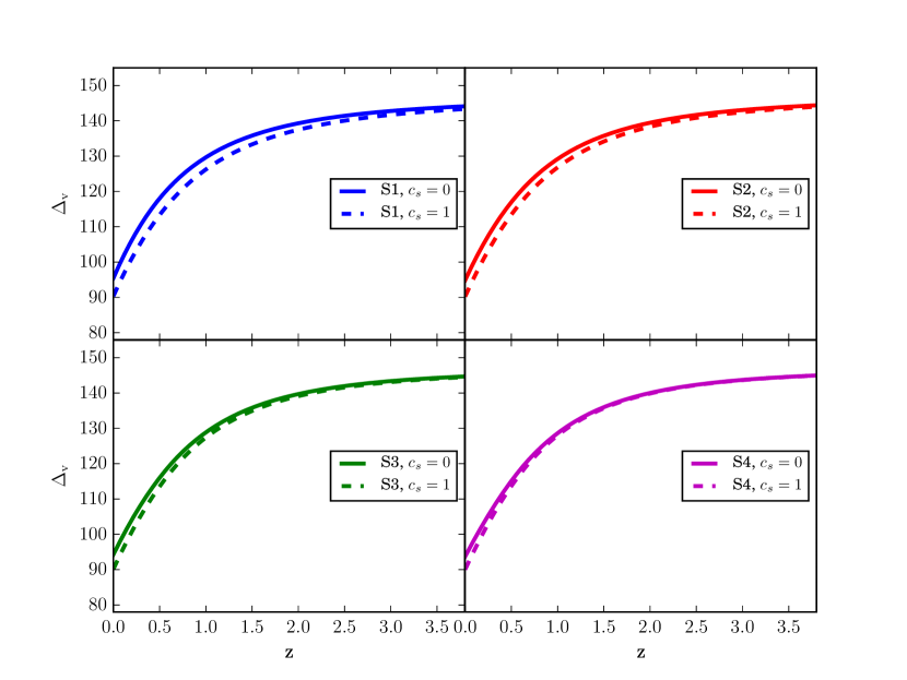
Figure 4: Virialization overdensity $\Delta_{{\rm v}}$ of Eq. (2.18) as function of redshift for the four sets of $w_{0}$ and $w_{a}$ given in Table 1.

2.3 Critical density threshold

Usually PS and ST mass functions make use of $\delta_{c}$ as the critical density threshold that defines collapsed regions. However, when DE perturbations are important, mass is not conserved and the sensible choice is to define the halo properties at the virialization time. Consequently, it seems inappropriate to use $\delta_{c}$ for the collapse threshold as in this case the mass function would depend on properties determined at the two different redshifts $z_{c}$ and $z_{{\rm v}}$. Therefore, we believe that the most natural quantity to use in the presence of DE fluctuations is the extrapolated linear contrast $\delta_{{\rm tot}}^{{\rm lin}}$ at the moment of virialization,

$$\delta_{{\rm v}}\left(z_{{\rm v}}\right)=\delta_{{\rm tot}}^{{\rm lin}}\left(z_{{\rm v}}\right)\,.$$ (2.19)

which we define as $\delta_{{\rm v}}$ in order to avoid confusion with the usual $\delta_{c}$. In Sec. 3 we show that this change can be absorbed into a redefinition of one parameter of the ST mass function.

In Fig. 5 we show the evolution of $\delta_{{\rm v}}$ as a function of $z$. As for the other quantities, the largest impact of DE fluctuations occur for S1. Note that, for both homogeneous and clustering DE, $\delta_{{\rm v}}$ grows as function of $z$, which is opposite to the usual behavior of $\delta_{c}$ (see, e.g., [35, 21, 22, 23]). The impact of DE fluctuations in $\delta_{{\rm v}}$ can be as large as 7% for S1, whereas the impact in the usual $\delta_{c}$ is at most 1% [23]. These results are valid only for DE with negligible $c_{s}$. For some range of small but non-negligible $c_{s}$, DE fluctuations are not negligible and can be treated linearly, [22]. In this case, the impact of DE fluctuations is smaller, but induces mass dependence, $\delta_{c}(z)\rightarrow\delta_{c}(z,M)$, which is not considered in this work.

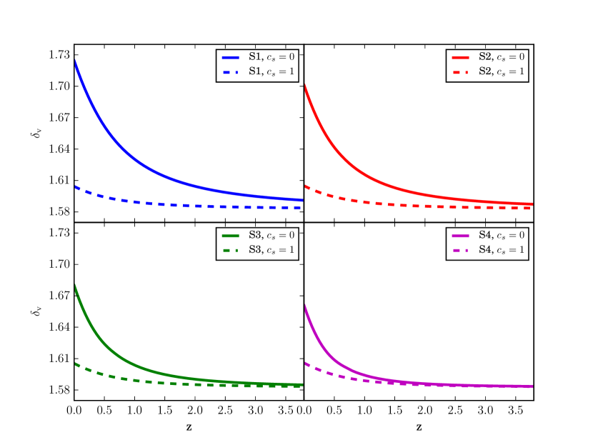
Figure 5: Critical contrast at virialization, $\delta_{{\rm v}}$, given by Eq. (2.18), as a function of redshift for the four sets of $w_{0}$ and $w_{a}$ given in Table 1. See Section 2.3 for more details.

3 Halo mass function

The halo mass function $f(M,z)$ gives the fraction of the total mass in halos of mass $M$ at redshift $z$. It is related to the (comoving) number density $n(M,z)$ by:

$$n(M,z)dM=\frac{\rho_{cc}(z)}{M}f(M,z)dM\,,$$ (3.1)

where $\rho_{cc}$ is the comoving average of the energy density that makes up the collapsed halos.

In the usual case of homogeneous DE $\rho_{cc}(z)=\rho_{mc}\equiv a^{3}\bar{\rho}_{m}$, where the latter is the constant matter density in a comoving volume and $a$ is the background scale factor.

The halo mass function acquires an approximate universality when expressed with respect to the variance of the mass fluctuations on a comoving scale $r$ at a given redshift $z$, $\Delta(r,z)$. The latter is given by:

$$\Delta^{2}(r,z)\,=\,\int_{0}^{\infty}\frac{dk}{k}\tilde{\Delta}^{2}(k,z)W^{2}(kr)\,,$$ (3.2)

where $W(kr)$ is the Fourier transform of the top-hat window function and $\tilde{\Delta}^{2}(k,z)$ is the dimensionless power spectrum extrapolated using linear theory to the redshift $z$:

$$\tilde{\Delta}^{2}(k,z)\equiv\frac{k^{3}}{2\pi^{2}}P(k,z)=\delta_{H0}^{2}\left(\frac{ck}{H_{0}}\right)^{3+n_{s}}T^{2}(k)\,G_{{\rm tot}}^{2}(z)\,.$$ (3.3)

In the previous equation $P(k,z)$ is the power spectrum, $n_{s}$ is the spectral index, $\delta_{H0}$ is the amplitude of perturbations on the horizon scale today, $G_{{\rm tot}}(z)$ is the normalized linear growth function given in Eq. (2.10) and $T(k)$ is the transfer function [36]. Note that the use of $G_{{\rm tot}}(z)$ accounts for the contribution of DE to the power spectrum. Since we are considering only the cases of $c_{s}=1$ and $c_{s}=0$, the transfer function shape should remain the same because DE perturbations are either negligible or have the same scale dependence of matter perturbations, thus changing only the overall normalization which is fixed via

$$\Delta(r=8h^{-1}\text{Mpc},z=0)=\sigma_{8}\,,$$ (3.4)

where $\sigma_{8}$ takes the fiducial value given earlier. Note that we are normalizing all the models to the same present-day value of $\sigma_{8}$. For the impact of general $c_{s}$ in the power spectrum see [37].

We model the mass function according to the functional form proposed by Sheth and Tormen (ST) [38]:

$$f_{{\rm ST}}(\Delta)=A\sqrt{\frac{2}{\pi}}\left[1+\left(\frac{\Delta^{2}}{a\delta_{c}^{2}}\right)^{p}\right]\frac{\sqrt{a}\delta_{c}}{\Delta}\exp\left[-\frac{a\delta_{c}^{2}}{2\Delta^{2}}\right].$$ (3.5)

In the previous equation $a$ and $p$ are free parameters while $A$ is fixed by the normalization condition $\int fdM=1$, according to which:

$$A=\left[1+\frac{2^{-p}}{\sqrt{\pi}}\Gamma(1/2-p)\right]^{-1}\,.$$ (3.6)

We adopt here the original values from [38], which are $a=0.707$ and $p=0.3$ and are expected to be approximately universal (see, however, [39]). In the case of clustering DE this is justified by the fact that for $c_{s}=0$ the shape of the power spectrum is not changed. However, we should point out that, to our knowledge, a numerical simulation that includes clustering DE has not yet been run and, therefore, the ST parameters $a$ and $p$ may depend on the DE properties. A possible change will likely increase the impact of inhomogeneous DE on the halo abundances. Consequently, by neglecting this effect our results will be more conservative.

We adopted the ST mass function as it depends on the peak height parameter $\nu=\delta_{c}/\Delta$ and not on $\Delta$ alone, as in the case of the precise mass function proposed by [1]. This makes the ST function more sensitive to the physics that goes into the halo collapse that we are studying in this paper. In order to obtain a more precise mass function, the usual approach – adopted, for example, in the context of non-Gaussianities [40] and baryonic feedback [41] – is to multiply the more precise but less cosmology-dependent mass functions by a correcting factor, which in our case is:

$$\frac{n(M,z)|_{c_{s}=0}}{n(M,z)|_{c_{s}=1}}=\frac{\rho_{cc}(z)f(M,z)|_{c_{s}=0}}{\rho_{mc}\,f(M,z)|_{c_{s}=1}}\,.$$ (3.7)

We shall then focus on this correcting factor when presenting our results.

As previously discussed, we define halos’ properties at the moment of virialization. The ST mass function, however, uses the critical contrast at collapse, $\delta_{c}$. Therefore, we need to adjust the parameter $a$ – which is degenerated with $\delta_{c}$ – in order to account for the different critical contrast used:

$$\tilde{a}\equiv a\frac{\delta_{c}^{2}}{\delta_{{\rm v}}^{2}}\simeq 0.803\,,$$ (3.8)

where within the EdS mode it is $\delta_{\rm v}\simeq 1.583$ and $\delta_{c}\simeq 1.686$. The ST mass function becomes:

$$f_{{\rm ST}}(\Delta)=A\sqrt{\frac{2}{\pi}}\left[1+\left(\frac{\Delta^{2}}{\tilde{a}\delta_{{\rm v}}^{2}}\right)^{p}\right]\frac{\sqrt{\tilde{a}}\delta_{{\rm v}}}{\Delta}\exp\left[-\frac{\tilde{a}\delta_{{\rm v}}^{2}}{2\Delta^{2}}\right].$$ (3.9)

Note that, because of the change of variable, $f_{{\rm ST}}$ is related to our original definition of $f$ by:

$$f(M,z)\,=\,f_{{\rm ST}}(\Delta)\frac{d\ln\Delta(M,z)^{-1}}{dM}\,.$$ (3.10)

In the latter, we have $\Delta(M,z)=\Delta(r(M,z),z)$, where the function $r(M,z)$ relates the comoving scale that collapsed to form the halo with the actual halo mass. Within homogeneous DE this relation is simply:

$$M=\frac{4\pi}{3}r^{3}\rho_{mc}\left(1+\delta_{m}\right)=\frac{4\pi}{3}r^{3}a^{3}\bar{\rho}_{m}\left(1+\delta_{m}\right)\,,$$ (3.11)

that is, thanks to mass conservation, one can take the mass corresponding to the collapsing sphere at early times when the perturbation is negligible and $\rho_{m}\approx\bar{\rho}_{m}$. Therefore, one get a “background level” relation $r=r(M)$ and it is not necessary to know the virialization time and the corresponding overdensity and halo radius.

As discussed in Section 2.2, when dark energy perturbations are present the total mass $M_{{\rm tot}}$ is not conserved. Hence, we need to define the actual halo mass and the radius at the virialization and the relation $r(M,z)$ is given by:

$$M_{{\rm tot}}=\frac{4\pi}{3}r^{3}b_{{\rm v}}^{3}(z)\Delta_{{\rm v}}(z)\bar{\rho}_{c}(z)\,,$$ (3.12)

where the physical halo radius is $R_{{\rm v}}\equiv r\,b_{{\rm v}}$, $b_{{\rm v}}(z)$ is independent of the comoving scale $r$ and so of the halo mass $M$. Considering $R_{i}=b_{i}r\simeq a_{i}r$, $b_{{\rm v}}$ can be computed using:

$$b_{{\rm v}}=\frac{R_{{\rm v}}a_{i}}{R_{i}}\,.$$ (3.13)

If only matter contributes to the mass, $M_{{\rm tot}}=M_{m}\left(z_{i}\right)=M_{m}\left(z_{{\rm v}}\right)$ is conserved and we can define the conserved $b_{{\rm v}}$ according to

$$\frac{4\pi}{3}r^{3}\rho_{mc}\left(1+\delta_{m}\left(z_{i}\right)\right)=\frac{4\pi}{3}r^{3}b_{{\rm v}}^{3}a^{-3}\rho_{mc}\left(1+\delta_{m}\left(z_{{\rm v}}\right)\right)$$

so that

$$b_{{\rm v}}^{{\rm cons}}=a_{{\rm v}}\left(\frac{1+\delta_{m}\left(z_{i}\right)}{1+\delta_{m}\left(z_{{\rm v}}\right)}\right)^{1/3}\,,$$ (3.14)

which is equal to the general case of Eq. (3.13) if dark energy fluctuations are negligible. We note that the common practice of neglecting $\delta_{m}\left(z_{i}\right)$ in (3.11) induces an error $\sim 0.1\%$ in $b_{{\rm v}}^{{\rm cons}}$. In Fig. 6 we show the evolution of the ratio $b_{{\rm v},c_{s}=0}/b_{{\rm v},c_{s}=1}$ for each set of parameterizations. In all cases, the modifications with respect to $b_{{\rm v}}^{{\rm cons}}$ grow with redshift. The largest differences occur for S3 and S4, a direct consequence of the impact of DE fluctuations on $R_{{\rm v}}$ as shown in Fig. 2.

Fig. 7 shows how different is the non-standard $r=r(M,z)$ relation with respect to the background relation $r=r(M)$ (left panel) and the impact of the non-standard $r=r(M,z)$ relation on the logarithmic derivative of (3.10). Here we only show the results for the case S1, which suffers the largest modifications. As one can see, the impact of clustering DE in the mass-scale relation is around 1% at $z=0$ (left panel of Fig. 7), however the actual impact on the mass function is one order of magnitude smaller because it depends on a logarithmic derivative (right panel of Fig. 7) and can be safely neglected.

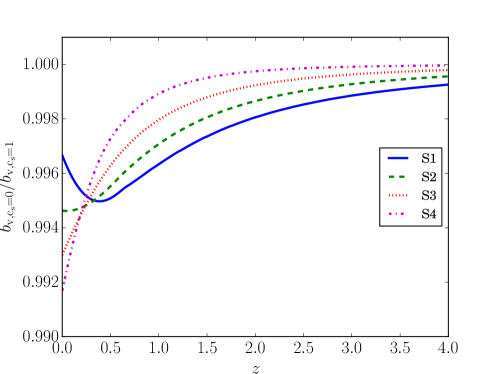
Figure 6: Plot of the ratio $b_{{\rm v},c_{s}=0}/b_{{\rm v},c_{s}=1}$ as function of redshift for the four sets of $w_{0}$ and $w_{a}$ given in Table 1. See Section 3 for more details.

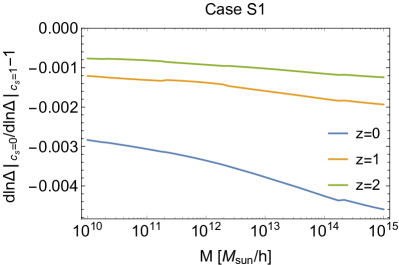
Figure 7: Left Panel: Fractional difference of the non-standard $r=r(M,z)$ relation from equation (3.12) with respect to the background relation $r=r(M)$. Right Panel: Impact of the non-standard $r=r(M,z)$ relation on the logarithmic derivative of (3.10). These plots refer to the set S1 given in Table 1.

Finally, the last quantity that we need to evaluate is $\rho_{cc}$. The total average mass density in halos at redshift $z$ can be obtained from the following equation:

$$\rho_{cc}(z) =\int M\,n(M,z){\rm d}M=\int M_{m}\,n(M,z){\rm d}M+\int M_{de}\,n(M,z){\rm d}M$$

$$=\int M_{m}\,n(M,z){\rm d}M+\epsilon(z)\int M_{m}\,n(M,z){\rm d}M=\rho_{mc}\,[1+\epsilon(z)]\,,$$ (3.15)

where it has been assumed that, at redshift $z$, all halos have the same ratio $\epsilon(z)$ given in Eq. (2.16). This neglects the fact that large halos are produced by the mergers of smaller halos that have virialized earlier and so with a different virialization overdensity and DE contribution. As we can see, the impact on the mass function is linear in $\epsilon$ (left panel of Fig. 3), so it increases abundances as much as 5% on all mass scales.

4 Results

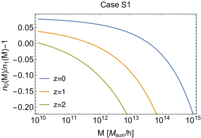
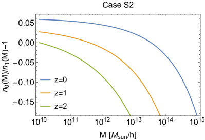
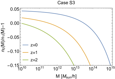
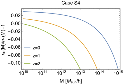
Figure 8: Fractional change in the mass function due to dark energy perturbations. $n_{0}(M)$ refers to dark energy with sound speed $c_{s}=0$, and similarly for $n_{1}(M)$. Perturbations are normalized today so that all models have the same $\sigma_{8}$. The four sets S1-4 of $w_{0}$ and $w_{a}$ are given in Table 1.

We show in Fig. 8 the quantity $\frac{n(M,z)|_{c_{s}=0}}{n(M,z)|_{c_{s}=1}}$ for the four sets of $w_{0}$ and $w_{a}$ given in Table 1 and at three different redshifts. As one can see, DE perturbations can impact halo abundances at the level of 10%–30%, depending on the halo mass and redshift. Bear in mind that all models have the same $\sigma_{8}$. In this case, clustering DE always diminishes the abundance of massive clusters $M>10^{14}M_{\odot}$. Interestingly, the number of small halos, $10^{10}M_{\odot}<M<10^{12}M_{\odot}$, is enhanced at $z=0$ and $z=1$. The main impact of clustering DE for large masses comes from the modifications in the quantity $\delta_{\rm{v}}/G_{{\rm tot}}$, which is always larger than in the homogeneous case and strongly reduces the number of halos around the exponential tail of the mass function. For small masses, the main impact is related to the density normalization of mass function, Eq. (3.15).

Had we normalized the amplitude of fluctuations at the redshift of CMB decoupling, clustering DE would have generated more massive clusters in comparison to homogeneous DE, therefore worsening the Planck Clusters tension. Clustering DE models alleviate this tension only if $w<-1$, in which case the impact of DE fluctuations is opposite to the case $w>-1$. However, as we discussed in Sect. 2.1, phantom clustering DE can generate negative energy densities, $\delta_{de}<-1$. We will address this problem in a forthcoming paper  [6].

There are numerous ongoing and planned surveys (e.g., DES [42, 43], J-PAS [44, 45], Euclid [46, 47, 48]) which will count the number of high-mass systems on the sky in an effort to better constrain the cosmological parameters that control the growth rate of structure. As we have seen the impact of DE perturbations on the mass function is greatest at large masses. Therefore, it is interesting to quantify how much cluster counts are affected by such perturbations.

Here, we neglect the effect of the mass-observable relation and we do not bin in mass. We will carry out survey-specific analyses in a forthcoming work. We define a cluster as an object with mass $M\geq M_{\rm thr}\equiv 10^{14}h^{-1}M_{\odot}$, a figure in agreement with the expected sensitivity from Euclid. The total number of clusters at the redshift $z$ and within the redshift bin $\Delta z$ is then:

$$N(z)\Delta z=\Delta z\frac{{\rm d}V}{{\rm d}z}\int_{M_{\rm thr}}^{\infty}{\rm d}M\,n(M,z)\,,$$ (4.1)

where the quantity ${\rm d}V/{\rm d}z$ is the cosmology-dependent comoving volume element per unit redshift interval which is given by:

$$\frac{{\rm d}V}{{\rm d}z}=4\pi(1+z)^{2}\,\frac{d_{A}^{2}(z)}{c^{-1}H(z)}\,,$$ (4.2)

where $d_{A}$ is the angular diameter distance and $H(z)$ is the Hubble rate at redshift $z$.

Figure 9 shows that cluster counts are modified by about 30% at a redshift of unity. Therefore, cluster counts is a very promising observable if one is to constrain models of dark energy that feature negligible sound speeds.

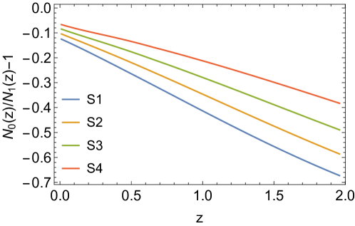
Figure 9: Fractional change in cluster number counts due to dark energy perturbations. $N(z)$ is computed using (4.1) and $N_{0}(z)$ refers to dark energy with sound speed $c_{s}=0$, and similarly for $N_{1}(z)$. Perturbations are normalized today so that all models have the same $\sigma_{8}$. The four sets S1-4 of $w_{0}$ and $w_{a}$ are given in Table 1.

5 Conclusions

In this paper we have discussed in detail how the halo mass function is modified when dark energy has a negligible sound speed that causes its perturbations to collapse. We have developed a consistent framework according to which the halo properties are defined at the moment of virialization and that takes into account the non-conservation of the mass relative to the dark-energy fluctuations.

To summarize, the corrections that directly impact the mass function due to the presence of DE fluctuations are :

• Growth function: based on the spherical collapse model in the radius approach, we have argued that the total perturbation density should be used, Eqs. (2.8) and (2.10). This new function differs from matter growth function in the homogeneous case by 3% to 8% for the equations of state we have analyzed.

• Threshold density for collapse: by demanding consistency in the definition of halo mass and the mass function quantities, we have argued that most natural threshold density to be used is the total linear perturbation density at the moment of virialization, $\delta_{{\rm v}}$, Eq. (2.19). The impact of clustering DE on this quantity is similar to the one on the growth function, but has a distinct redshift evolution in comparison with the usual $\delta_{c}$.

• Mass-scale relation: since the total mass of a halo with some fraction of DE fluctuation is not conserved, one can not use the background mass-scale relation for matter only. The corrected relation is given by Eqs. (3.12) and (3.13). This, however, is a sub-percent correction and can be safely neglected.

• Normalization density: also because DE fluctuations induce non-conservation of total mass, the mean energy density that normalizes the mass function has to be corrected, Eq. (3.15). This is a linear modification of the order of the DE mass fraction $\epsilon$ and so it changes the mass function by a few % on all mass scales.

We have then computed the impact of clustering dark energy considering all the mentioned modifications on the mass function and found that halo abundances can be altered at the level of 10%–30%, depending on the halo mass and redshift. As the change is largest at the high masses of galaxy clusters, we have then computed the impact on cluster number counts and obtained that they are modified by about 30% at a redshift of unity, as big an effect as the one that comes from including baryons within cosmological simulations [41]. A comprehensive analysis that takes into account the nuisances from the scaling relations will be the subject of forthcoming work [6].

References

- [1] J. L. Tinker, A. V. Kravtsov, A. Klypin, K. Abazajian, M. S. Warren, G. Yepes et al., Toward a halo mass function for precision cosmology: The Limits of universality, Astrophys. J. 688 (2008) 709–728, [0803.2706].
- [2] E. Rozo, R. H. Wechsler, B. P. Koester, T. A. McKay, A. E. Evrard et al., Cosmological constraints from sdss maxbcg cluster abundances, Astrophys.J. (2007) , [astro-ph/0703571].
- [3] A. Mantz, S. W. Allen, H. Ebeling and D. Rapetti, New constraints on dark energy from the observed growth of the most X-ray luminous galaxy clusters, Mon. Not. Roy. Astron. Soc. 387 (2008) 1179–1192, [0709.4294].
- [4] A. Vikhlinin et al., Chandra cluster cosmology project iii: Cosmological parameter constraints, Astrophys. J. 692 (2009) 1060–1074, [0812.2720].
- [5] Planck collaboration, P. A. R. Ade et al., Planck 2015 results. XXIV. Cosmology from Sunyaev-Zeldovich cluster counts, Astron. Astrophys. 594 (2016) A24, [1502.01597].
- [6] R. C. Batista and V. Marra, Clustering dark energy and Planck cluster counts, in preparatiion (2017) .
- [7] M. A. Amin, P. Zukin and E. Bertschinger, Scale-Dependent Growth from a Transition in Dark Energy Dynamics, Phys.Rev. D85 (2012) 103510, [1108.1793].
- [8] T. Padmanabhan, Accelerated expansion of the universe driven by tachyonic matter, Phys. Rev. D66 (2002) 021301, [hep-th/0204150].
- [9] J. S. Bagla, H. K. Jassal and T. Padmanabhan, Cosmology with tachyon field as dark energy, Phys. Rev. D67 (2003) 063504, [astro-ph/0212198].
- [10] J. Garriga and V. F. Mukhanov, Perturbations in k-inflation, Phys. Lett. B458 (1999) 219–225, [hep-th/9904176].
- [11] C. Armendariz-Picon, V. F. Mukhanov and P. J. Steinhardt, Essentials of k essence, Phys.Rev. D63 (2001) 103510, [astro-ph/0006373].
- [12] E. A. Lim, I. Sawicki and A. Vikman, Dust of Dark Energy, JCAP 1005 (2010) 012, [1003.5751].
- [13] P. Creminelli, G. D’Amico, J. Norena and F. Vernizzi, The effective theory of quintessence: the w<-1 side unveiled, JCAP 0902 (2009) 018, [0811.0827].
- [14] J. E. Gunn and J. R. I. Gott, On the infall of matter into cluster of galaxies and some effects on their evolution, Astrophys. J. 176 (1972) 1–19.
- [15] W. H. Press and P. Schechter, Formation of galaxies and clusters of galaxies by selfsimilar gravitational condensation, Astrophys. J. 187 (1974) 425–438.
- [16] R. K. Sheth, H. J. Mo and G. Tormen, Ellipsoidal collapse and an improved model for the number and spatial distribution of dark matter haloes, Mon. Not. Roy. Astron. Soc. 323 (2001) 1, [astro-ph/9907024].
- [17] D. F. Mota and C. van de Bruck, On the spherical collapse model in dark energy cosmologies, Astron. Astrophys. 421 (2004) 71–81, [astro-ph/0401504].
- [18] M. Manera and D. F. Mota, Cluster number counts dependence on dark energy inhomogeneities and coupling to dark matter, Mon. Not. Roy. Astron. Soc. 371 (2006) 1373, [astro-ph/0504519].
- [19] L. Abramo, R. Batista, L. Liberato and R. Rosenfeld, Structure formation in the presence of dark energy perturbations, JCAP 0711 (2007) 012, [0707.2882].
- [20] L. Abramo, R. Batista, L. Liberato and R. Rosenfeld, Physical approximations for the nonlinear evolution of perturbations in inhomogeneous dark energy scenarios, Phys.Rev. D79 (2009) 023516, [0806.3461].
- [21] P. Creminelli, G. D’Amico, J. Norena, L. Senatore and F. Vernizzi, Spherical collapse in quintessence models with zero speed of sound, JCAP 1003 (2010) 027, [0911.2701].
- [22] T. Basse, O. E. Bjaelde and Y. Y. Y. Wong, Spherical collapse of dark energy with an arbitrary sound speed, JCAP 1110 (2011) 038, [1009.0010].
- [23] R. Batista and F. Pace, Structure formation in inhomogeneous Early Dark Energy models, JCAP 1306 (2013) 044, [1303.0414].
- [24] F. Pace, R. C. Batista and A. Del Popolo, Effects of shear and rotation on the spherical collapse model for clustering dark energy, Mon.Not.Roy.Astron.Soc. 445 (2014) 648, [1406.1448].
- [25] C. Heneka, D. Rapetti, M. Cataneo, A. B. Mantz, S. W. Allen and A. von der Linden, Cold dark energy constraints from the abundance of galaxy clusters, 1701.07319.
- [26] E. Sefusatti and F. Vernizzi, Cosmological structure formation with clustering quintessence, JCAP 1103 (2011) 047, [1101.1026].
- [27] M. Fasiello and Z. Vlah, Nonlinear fields in generalized cosmologies, Phys. Rev. D94 (2016) 063516, [1604.04612].
- [28] M. Fasiello and Z. Vlah, On Observables in a Dark Matter-Clustering Quintessence System, 1611.00542.
- [29] D. Herrera, I. Waga and S. E. Jorás, Calculation of the critical overdensity in the spherical-collapse approximation, Phys. Rev. D95 (2017) 064029, [1703.05824].
- [30] F. Pace, S. Meyer and M. Bartelmann, On the implementation of the spherical collapse model for dark energy models, 1708.02477.
- [31] R. C. Batista, Impact of dark energy perturbations on the growth index, Phys.Rev. D89 (2014) 123508, [1403.2985].
- [32] L. R. W. Abramo, R. Batista, L. Liberato and R. Rosenfeld, Dynamical Mutation of Dark Energy, Phys.Rev. D77 (2008) 067301, [0710.2368].
- [33] T. Basse, O. E. Bjaelde, S. Hannestad and Y. Y. Y. Wong, Confronting the sound speed of dark energy with future cluster surveys, 1205.0548.
- [34] S. Lee and K.-W. Ng, Spherical collapse model with non-clustering dark energy, JCAP 1010 (2010) 028, [0910.0126].
- [35] F. Pace, J. C. Waizmann and M. Bartelmann, Spherical collapse model in dark energy cosmologies, arXiv:1005.0233 [astro-ph.CO] (2010) .
- [36] D. J. Eisenstein and W. Hu, Baryonic features in the matter transfer function, Astrophys. J. 496 (1998) 605, [astro-ph/9709112].
- [37] M. Kunz, S. Nesseris and I. Sawicki, Using dark energy to suppress power at small scales, Phys. Rev. D92 (2015) 063006, [1507.01486].
- [38] R. K. Sheth and G. Tormen, Large-scale bias and the peak background split, MNRAS 308 (Sept., 1999) 119–126, [arXiv:astro-ph/9901122].
- [39] T. Castro, V. Marra and M. Quartin, Constraining the halo mass function with observations, Mon.Not.Roy.Astron.Soc. 463 (2016) 1666–1677, [1605.07548].
- [40] M. LoVerde, A. Miller, S. Shandera and L. Verde, Effects of Scale-Dependent Non-Gaussianity on Cosmological Structures, JCAP 0804 (2008) 014, [0711.4126].
- [41] M. Velliscig, M. P. van Daalen, J. Schaye, I. G. McCarthy, M. Cacciato, A. M. C. Le Brun et al., The impact of galaxy formation on the total mass, mass profile and abundance of haloes, Mon. Not. Roy. Astron. Soc. 442 (2014) 2641–2658, [1402.4461].
- [42] Dark Energy Survey collaboration, T. Abbott et al., The dark energy survey, astro-ph/0510346.
- [43] DES collaboration, T. M. C. Abbott et al., Dark Energy Survey Year 1 Results: Cosmological Constraints from Galaxy Clustering and Weak Lensing, 1708.01530.
- [44] J-PAS collaboration, N. Benitez et al., J-PAS: The Javalambre-Physics of the Accelerated Universe Astrophysical Survey, 1403.5237.
- [45] B. Ascaso et al., An Accurate Cluster Selection Function for the J-PAS Narrow-Band wide-field survey, Mon. Not. Roy. Astron. Soc. 456 (2016) 4291–4304, [1601.00656].
- [46] EUCLID collaboration, R. Laureijs et al., Euclid Definition Study Report, 1110.3193.
- [47] B. Sartoris et al., Next Generation Cosmology: Constraints from the Euclid Galaxy Cluster Survey, Mon. Not. Roy. Astron. Soc. 459 (2016) 1764–1780, [1505.02165].
- [48] L. Amendola et al., Cosmology and Fundamental Physics with the Euclid Satellite, 1606.00180.