Conjugate gradient based acceleration for inverse problems

Abstract

The conjugate gradient method is a widely used algorithm for the numerical solution of a system of linear equations. It is particularly attractive because it allows one to take advantage of sparse matrices and produces (in case of infinite precision arithmetic) the exact solution after a finite number of iterations. It is thus well suited for many types of inverse problems. On the other hand, the method requires the computation of the gradient. Here difficulty can arise, since the functional of interest to the given inverse problem may not be differentiable. In this paper, we review two approaches to deal with this situation: iteratively reweighted least squares and convolution smoothing. We apply the methods to a more generalized, two parameter penalty functional. We show advantages of the proposed algorithms using examples from a geotomographical application and for synthetically constructed multi-scale reconstruction and regularization parameter estimation.

1 Introduction

Consider the linear system $Ax=b$, where $A\in\mathbb{R}^{m\times n}$ and $b\in\mathbb{R}^{m}$. Often, in linear systems arising from physical inverse problems, we have more unknowns than data: $m\ll n$ [19] and the right hand side of the system corresponding to the observations or measurements is noisy. In such a setting, it is common to use regularization by introducing a constraint on the solution, both to account for the possible ill-conditioning of $A$ and noise in $b$ and for the lack of data with respect to the number of unknown variables in the linear system. A commonly used constraint is imposed via a penalty on the norm of the solution, either forcing the sum of certain powers of the absolute values of coefficients to be bounded or for many of the coefficients to be zero, i.e. sparsity: to require the solution $x$ to have few nonzero elements compared to the dimension of $x$. To account for different kinds of scenarios, we consider here the generalized functional:

$$F_{l,p}(x)=\|Ax-b\|_{l}^{l}+\lambda\|x\|_{p}^{p}=\displaystyle\sum_{i=1}^{m}\left|\displaystyle\sum_{j=1}^{n}A_{ij}x_{j}-b_{i}\right|^{l}+\lambda\sum_{k=1}^{n}|x_{k}|^{p},$$ (1.1)

for $1\leq l,p\leq 2$. For example, when $l=p=2$, the familiar Tikhonov regularization is recovered. When $l=2$ and $p=1$, we obtain the least squares problem with the convex $\ell_{1}$ regularizer, governed by the regularization parameter $\lambda>0$ [5], commonly used for sparse signal recovery. In addition, (1.1) allows us to impose a non-standard penalty on the residual vector, $r=Ax-b$. This is useful e.g. in cases, where we want to impose a higher penalty on any outliers which may be present in $b$. (Since the $l=2$ case is commonly utilized, we denote $\tilde{F}_{p}(x):=F_{2,p}(x)$). For any $p\geq 1$, the map $\|x\|_{p}:=\left(\sum_{k=1}^{n}|x_{k}|^{p}\right)^{\frac{1}{p}}$ (for any $x\in\mathbb{R}^{n}$) is called the $\ell_{p}$-norm on $\mathbb{R}^{n}$. For $p=1$, the $\|\cdot\|_{1}$ norm is called an $\ell_{1}$ norm and is convex. As $p\to 0$, the right term of this functional approximates the count of nonzeros or the so-called $\ell_{0}$ “norm”:

$$\|x\|_{0}=\lim_{p\to 0}\|x\|_{p}=\lim_{p\to 0}\left(\sum_{k=1}^{n}|x_{k}|^{p}\right)^{1/p}.$$

For different $p$ values this measure is plotted in Figure 1.

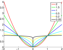
Figure 1: $|x|^{p}$ plotted for different values of $p$; as $p\to 0$, the plot approaches an indicator function.

The non-smoothness of the family of functionals $F_{l,p}(x)$ complicates their minimization from an algorithmic point of view. The non-smooth part of (1.1) is due to the absolute value function $g(x_{k})=|x_{k}|$ or of $h(r_{k})=|(Ax-b)_{k}|$, or both, depending on the values of $l$ and $p$. Because the gradient of $F_{l,p}(x)$ cannot be obtained when $l$ or $p$ are less than $2$, different minimization techniques such as sub-gradient methods are frequently used [18]. For the convex $l=2,p=1$ case in (1.1), various thresholding based methods have become popular. A particularly successful example is the soft thresholding based method FISTA [2]. This algorithm is an accelerated version of a soft thresholded Landweber iteration [11]:

$$x^{n+1}=\mathbb{S}_{\frac{\lambda}{2}}(x^{n}+A^{T}b-A^{T}Ax^{n}).$$ (1.2)

The soft thresholding function $\mathbb{S}_{\lambda}:\mathbb{R}^{n}\to\mathbb{R}^{n}$ [5] is defined by

$$\left(\mathbb{S}_{\lambda}(x)\right)_{k}=\operatorname{sgn}(x_{k})\max{\{0,|x_{k}|-\lambda\}},\ \forall\,k=1,\ldots,n,\ \forall\,x\in\mathbb{R}^{n}.$$

The scheme (1.2) is known to converge from some initial guess, but slowly, to the $\ell_{1}$ minimizer [5]. The thresholding in (1.2) is performed on $x^{n}-\nabla_{x}(\frac{1}{2}\|Ax^{n}-b\|_{2}^{2})=x^{n}-A^{T}(Ax^{n}-b)$, which is a very simple gradient based scheme with a constant line search [8]. The thresholding based schemes typically require many iterations to converge and this is costly (due to the many matrix-vector mults required) when $A$ is large. Moreover, the regularization parameter $\lambda$ is often not known in advance. Instead, it is frequently estimated using a variant of the L-curve technique [10] together with a continuation scheme, where $\lambda$ is iteratively decreased, reusing the previous solution as the initial guess at the next lower $\lambda$. This requires many iterations.

In this article, we discuss two approaches to obtaining approximate solutions to (1.1) using an accelerated conjugate gradient approach, with a specific focus on the case of large matrix $A$, where the use of thresholding based techniques is expensive, due to the many iterations required. In contrast, our methods accomplish similar work in fewer iterations, because each iteration is more powerful than that of a thresholding scheme. We consider specifically the case $1\leq l,p\leq 2$ since for $0<l,p<1$, (1.1) is not convex. However, the minimization of non-smooth non-convex functions has been shown to produce good results in some compressive sensing applications [4] and our methods can be applied also to the non-convex case, as long as care is taken to avoid local minima.

The first approach is based on the conjugate gradient acceleration of the reweighted least squares idea developed in [20] with further developments and analysis given in [9]. The approach is based on a two norm approximation of the absolute value function:

$$|x_{k}|=\frac{x_{k}^{2}}{|x_{k}|}=\frac{x_{k}^{2}}{\sqrt{x_{k}^{2}}}\approx\frac{x_{k}^{2}}{\sqrt{x_{k}^{2}+\epsilon^{2}}}$$

where in the rightmost term, a small $\epsilon\neq 0$ is used, to insure the denominator is finite, regardless of the value of $x_{k}$. Thus, at the $n$-th iteration, a reweighted $\ell_{2}$-approximation to the $\ell_{1}$-norm of $x$ is of the form:

$$\|x\|_{1}\approx\displaystyle\sum_{k=1}^{N}\frac{x_{k}^{2}}{\sqrt{(x^{n}_{k})^{2}+\epsilon_{n}^{2}}}=\displaystyle\sum_{k=1}^{N}\tilde{w}^{n}_{k}x_{k}^{2}$$

where the right hand side is a reweighted two-norm with weights:

$$\tilde{w}^{n}_{k}=\frac{1}{\sqrt{(x^{n}_{k})^{2}+\epsilon_{n}^{2}}}.$$

It follows that $\sum_{k}\tilde{w}^{n}_{k}(x^{n}_{k})^{2}$ is a close approximation to $\|x^{n}\|_{1}$, which proceeds to $\|x\|_{1}$ as $n\to\infty$. Given the smooth approximation resulting from the reweighted two norm, the gradient acceleration idea is then built on top of the least squares approximations. A slight generalization of the weights makes the approach applicable to (1.1) with $l=2$. With the aid of results from [16] and the assumption that the residuals are nonzero, we are able to extend the algorithm to the general case in (1.1).

The second approach is based on smooth approximations to the non-smooth absolute value function $g(t)=|t|$, computed via convolution with a Gaussian function, described in detail in [22]. Starting from the case $l=2$, we replace the non-smooth objective function $\tilde{F}_{p}(x)$ by a smooth functional $H_{p,\sigma}(x)$, which is close to $\tilde{F}_{p}(x)$ in value (as the parameter $\sigma\to 0$). Since the approximating functional $H_{p,\sigma}(x)$ is smooth, we can compute its gradient vector $\nabla_{x}H_{p,\sigma}(x)$ and Hessian matrix $\nabla^{2}_{x}H_{p,\sigma}(x)$. We are then able to use gradient based algorithms such as conjugate gradients to approximately minimize $\tilde{F}_{p}(x)$ by working with the approximate functional and gradient pair. We also apply the approach to the general case (where we may have $l\neq 2$) in (1.1), with the assumption that the residuals are nonzero.

In this paper, we describe the use of both acceleration approaches and the generalized functional, and give some practical examples from Geophysics and of wavelet based model reconstructions.

2 Iteratively Reweighted Least Squares

The iteratively reweighted least squares (IRLS) method, was originally presented in [6]. The algorithm presented here is from the work in [20]. Several new developments have recently emerged. In particular, [9] provides the derivations for the practical implementation of the IRLS CG scheme (without running the CG algorithm to convergence at each iteration) while [3] provides some stability and convergence arguments in the presence of noise. In this article, we survey the method and present the extension of the algorithm to (1.1), without going into the mathematical details for the convergence arguments, which are provided in the above references and can be extended to (1.1) with our assumptions. The basic idea of IRLS consists of a series of smooth approximations to the absolute value function:

$$\|x\|_{1}\approx\displaystyle\sum_{k=1}^{N}\frac{x_{k}^{2}}{\sqrt{(x^{n}_{k})^{2}+\epsilon_{n}^{2}}}=\displaystyle\sum_{k=1}^{N}\tilde{w}^{n}_{k}x_{k}^{2}$$

where the right hand side is a reweighted two-norm with weights:

$$\tilde{w}^{n}_{k}=\frac{1}{\sqrt{(x^{n}_{k})^{2}+\epsilon_{n}^{2}}}.$$ (2.1)

In [21], the non-CG version of the IRLS algorithm is considered with the generalized weights:

$$w^{n}_{k}=\frac{1}{\left[(x^{n}_{k})^{2}+\epsilon_{n}^{2}\right]^{\frac{2-p}{2}}}.$$ (2.2)

This results in the iterative scheme:

$$x^{n+1}_{k}=\frac{1}{1+\frac{1}{2}\lambda pw^{n}_{k}}\left(x^{n}_{k}+(A^{T}b)_{k}-(A^{T}Ax^{n})_{k}\right)\quad\mbox{for}\quad k=1,\dots,N,$$ (2.3)

which converges to the minimizer of (1.1) for $l=2$ and $1\leq p\leq 2$. The iteratively reweighted least squares (IRLS) algorithm given by scheme (2.3) with weights (2.2) follows from the construction of a surrogate functional (2.5), as per Lemma 2.1 below.

Lemma 2.1

Define the surrogate functional:

$$\quad G(x,a,w,\epsilon) = \|Ax-b\|_{2}^{2}-\|A(x-a)\|_{2}^{2}+\|x-a\|_{2}^{2}$$ (2.4)

$$+ \displaystyle\sum\frac{1}{2}\lambda\left(pw_{k}\left((x_{k})^{2}+\epsilon^{2}\right)+(2-p)(w_{k})^{\frac{p}{p-2}}\right)$$ (2.5)

where $\epsilon_{n}=\min\left(\epsilon_{n-1},(\|x^{n}-x^{n-1}\|_{2}+\alpha)^{\frac{1}{2}}\right)$ with $\alpha\in(0,1)$. Then the minimization procedure $~{}w^{n}=\arg\min_{w}G(x^{n},a,w,\epsilon_{n})~{}$ defines the iteration dependent weights:

$$w^{n}_{k}=\frac{1}{\left[(x^{n}_{k})^{2}+\epsilon_{n}^{2}\right]^{\frac{2-p}{2}}}.$$ (2.6)

In addition, the minimization procedure $x^{n+1}=\arg\min_{x}G(x,x^{n},w^{n},\epsilon_{n})$, produces the iterative scheme:

$$x^{n+1}_{k}=\frac{1}{1+\frac{1}{2}\lambda pw^{n}_{k}}\left((x^{n})_{k}-(A^{T}Ax^{n})_{k}+(A^{T}b)_{k}\right).$$ (2.7)

which converges to the minimizer of (1.1) for $l=2$ and $1\leq p\leq 2$.

The proof of the lemma is given in [21]. The construction of the non-increasing sequence $(\epsilon_{n})$ is important for convergence analysis. On the other hand, different choices can be used for implementations. The auxiliary $G(\dots)$ function is also used for the convergence proof and for the derivation of the algorithm. In particular, it is chosen to yield $\|x^{n}-x^{n-1}\|\to 0$ and to conclude the boundedness of the sequence of iterates $(x^{n})$. In the same paper, the FISTA style acceleration of the scheme is shown. In practice, however, a large number of iterations may be required for convergence and so the CG acceleration of the above scheme is of particular interest.

2.1 Conjugate gradient acceleration

Acceleration via CG is accomplished by modifying the auxiliary functional (2.4). If we instead set,

$$G(x,w,\epsilon)=\|Ax-b\|_{2}^{2}+\lambda\displaystyle\sum_{k=1}^{N}\left[pw_{k}\left(x_{k}^{2}+\epsilon^{2}\right)+(2-p)w_{k}^{\frac{p}{p-2}}\right],$$

then the two minimization problems:

$$w^{n+1}=\arg\min_{w}G(x^{n+1},w,\epsilon_{n+1})\quad;\quad x^{n+1}=\arg\min_{x}G(x,w^{n},\epsilon_{n})$$

give the same iteration dependent weights in (2.6) and the iterative scheme:

$$x^{n+1}=\arg\min_{x}\left\{\|Ax-b\|_{2}^{2}+\frac{1}{2}\lambda p\displaystyle\sum_{k=1}^{N}w^{n}_{k}x_{k}^{2}\right\}.$$ (2.8)

The details of convergence are given in [20]. The choice of the non-increasing $(\epsilon_{n})$ sequence is again crucial for convergence analysis, although simpler choices (e.g. $\epsilon_{n}=\|x^{n}-x^{n-1}\|$ can be programmed in practice). The choice

$$\epsilon^{n}=\min\left(\epsilon^{n-1},|G(x^{n-2},w^{n-2},\epsilon_{n-2})-G(x^{n-1},w^{n-1},\epsilon_{n-1})|^{\frac{\gamma}{2}}+\alpha^{n}\right),$$ (2.9)

with $\alpha\in(0,1)$ and $0<\gamma<\frac{2}{4-p^{2}}$ is taken for showing convergence to the minimizer in [20].

We now look more closely at the optimization problem in (2.8) above. In particular, notice that we can write:

$$\sum_{k=1}^{N}\frac{1}{2}\lambda pw^{n}_{k}x_{k}^{2}=\displaystyle\sum_{k=1}^{N}(D^{n}_{kk})^{2}x_{k}^{2}=\|D^{n}x\|_{2}^{2}$$

where $D^{n}$ is an iteration dependent diagonal matrix with elements $D^{n}_{kk}=\sqrt{\frac{1}{2}\lambda pw^{n}_{k}}$. This observation allows us to write the solution to the optimization problem at each iteration in terms of a linear system:

$$x^{n+1}=\arg\min_{x}\left\{\|Ax-b\|_{2}^{2}+\|D^{n}x\|_{2}^{2}\right\}\implies\left(A^{T}A+(D^{n})^{T}(D^{n})\right)x^{n+1}=A^{T}b.$$ (2.10)

In turn, the system in (2.10) can be solved using CG iterations. In practice, we need only an approximate solution to the above linear system at each iteration so the amount of CG iterations can be less than $5$ at each iteration $n$. In [9], it is shown that this procedure (involving inexact CG solutions) gives convergence to the minimizer. Notice also that it is not necessary to build up the $D^{n}$ matrix. Instead, the matrix is applied to vectors at each iteration, which can be done using an array computation. In [20], the application of the Woodbury matrix identity is explored, which can aid in cases where IRLS is applied to short and wide or tall and thin matrices.

2.2 Application to generalized residual penalty

Next, we consider the application of the IRLS scheme to (1.1). In [16] an IRLS algorithm for the minimization of $\min_{x}\displaystyle\sum_{i=1}^{m}\left|\displaystyle\sum_{j=1}^{n}A_{ij}x_{j}-b_{i}\right|^{l}$ was developed. The generalized IRLS equations resulting from this problem are $A^{T}R^{n}Ax^{n+1}=A^{T}R^{n}b$, where $R^{n}$ is a diagonal matrix with elements $l|r^{n}_{i}|^{l-2}$, where $r^{n}_{i}=(Ax^{n}-b)_{i}=\displaystyle\sum_{j=1}^{n}A_{ij}x_{j}-b_{i}$. This system was derived by setting the gradient to zero where it was assumed that $r_{i}\neq 0$ for all $i$. In this case [16]:

$$\frac{\partial}{\partial x_{k}}\displaystyle\sum_{i=1}^{m}|r_{i}(x)|^{l}=\displaystyle\sum_{i=1}^{m}l\operatorname{sgn}(r_{i})|r_{i}|^{l-1}A_{ik}=\displaystyle\sum_{i=1}^{m}r_{i}l|r_{i}|^{l-2}A_{ik}=[A^{T}R(Ax-b)]_{k}$$ (2.11)

where we make use of $\operatorname{sgn}(r_{i})=\frac{r_{i}}{|r_{i}|}$. When $l=2$, the familiar normal equations are recovered. Notice that $r_{i}\neq 0$ for all $i$ is a strong but plausible assumption to make (for example, to enforce this, we can add a very small amount of additive noise to the right hand side; the effect of noise on stability and convergence of IRLS has been analyzed in [3]). However, the same cannot be said of $x_{i}$ e.g. for sparse solutions, where many components can equal zero. If, with the assumption $r_{i}\neq 0$ for all $i$, we use the surrogate functional,

$$\tilde{G}(x,w,\epsilon)=\displaystyle\sum_{i=1}^{m}\left|\displaystyle\sum_{j=1}^{n}A_{ij}x_{j}-b_{i}\right|^{l}+\lambda\displaystyle\sum_{k=1}^{N}\left[pw_{k}\left(x_{k}^{2}+\epsilon^{2}\right)+(2-p)w_{k}^{\frac{p}{p-2}}\right]$$

it then follows that the resulting algorithm for the minimization of (1.1) can be written as:

$$\left(A^{T}R^{n}A+(D^{n})^{T}(D^{n})\right)x^{n+1}=A^{T}R^{n}b$$ (2.12)

with the same diagonal matrix $D^{n}$ as before and with the diagonal matrix $R^{n}$ with diagonal elements $|r^{n}_{i}|^{l-2}$ (for $i$ where $|r^{n}_{i}|<\epsilon$, we can set the entry to $\epsilon^{l-2}$ with the choice of $\epsilon$ user controllable, tuned for a given application). As before, at each iteration $n$, the system in (2.12) can be solved (approximately) using a few iterations of the CG algorithm (or some variant of the method, such as LSQR [13]). Below, we present the basic version of the IRLS CG algorithm. In practice, the parameter sequence $\epsilon_{n}$ for $D$ can be set to e.g. $\|x^{n}-x^{n-1}\|$ or the update in (2.9) can be used. Fixing $\epsilon$ for $R$ is common. Varying it may be useful in the case that $p$ or $l$ less than $1$ are chosen, resulting in a non-convex problem. For large problems it is important not to form $D$ and $R$ matrices explicitly. Instead vectors $\vec{d}$ and $\vec{r}$ can be used to hold their diagonal elements (i.e. $D^{n}x=\vec{d}^{n}\circ x$).

Input : An $m\times n$ matrix $A$, an initial guess $n\times 1$ vector $x^{0}$, a parameter $\lambda<\|A^{T}b\|_{\infty}$, a parameter $l\in[1,2]$, a parameter $p\in[1,2]$, a parameter $\epsilon\in(0,1)$, a maximum number of iterations to perform $N$ and a maximum number of local CG iterations to perform $N_{l}$.

Output : A vector $\bar{x}$, close to either the global or local minimum of $F_{l,p}(x)$, depending on choice of $p,l$.

Set $\epsilon_{1}=\epsilon$.

for $n=1,\dots N$ do

       Set weights $w^{n}_{k}=\frac{1}{\left[(x^{n}_{k})^{2}+\epsilon_{n}^{2}\right]^{\frac{2-p}{2}}}$.

       Initialize vectors $\vec{d}^{n}$ and $\vec{r}^{n}$ for the diagonal elements of diagonal matrices $D^{n}$ and $R^{n}$, with $\vec{d}^{n}_{k}=\sqrt{\frac{1}{2}\lambda pw^{n}_{k}}$ and $\vec{r}^{n}_{k}=l|r_{k}|^{l-2}$, with $r_{k}=(Ax^{n}-b)_{k}$, for $|r_{k}|>\epsilon$; and $r^{n}_{k}=l|\epsilon|^{l-2}$ for $|r_{k}|<\epsilon$.

       Run $N_{l}$ iterations of CG on the system $\left(A^{T}R^{n}A+(D^{n})^{T}(D^{n})\right)x^{n+1}=A^{T}R^{n}b$.

       Compute $\epsilon_{n+1}$.

end for

Algorithm 1 IRLS CG Algorithm

3 Approximate mollifier approach via convolution

In mathematical analysis, a smooth function $\psi_{\sigma}:\mathbb{R}\to\mathbb{R}$ is said to be a (non-negative) mollifier if it has finite support, is non-negative $(\psi\geq 0)$, and has area $\int_{\mathbb{R}}\psi(t)\mathrm{d}t=1$ [7]. For any mollifier $\psi$ and any $\sigma>0$, define the parametric function $\psi_{\sigma}:\mathbb{R}\to\mathbb{R}$ by: $\psi_{\sigma}(t):=\frac{1}{\sigma}\psi\left(\frac{t}{\sigma}\right)$, for all $t\in\mathbb{R}$. Then $\{\psi_{\sigma}:\sigma>0\}$ is a family of mollifiers, whose support decreases as $\sigma\to 0$, but the volume under the graph always remains equal to one. We then have the following important lemma for the approximation of functions, whose proof is given in [7].

Lemma 3.1

For any continuous function $g\in L^{1}(\Theta)$ with compact support and $\Theta\subseteq\mathbb{R}$, and any mollifier $\psi:\mathbb{R}\to\mathbb{R}$, the convolution $\psi_{\sigma}*g$, which is the function defined by:

$$(\psi_{\sigma}*g)(t):=\int_{\mathbb{R}}\psi_{\sigma}(t-s)g(s)\mathrm{d}s=\int_{\mathbb{R}}\psi_{\sigma}(s)g(t-s)\mathrm{d}s,\ \forall\,t\in\mathbb{R},$$

converges uniformly to $g$ on $\Theta$, as $\sigma\to 0$.

3.1 Smooth approximation to the absolute value function

Motivated by the above results, we will use convolution with approximate mollifiers to approximate the absolute value function $g(t)=|t|$ (which is not in $L^{1}(\mathbb{R})$) with a smooth function. We start with the Gaussian function $K(t)=\frac{1}{\sqrt{2\pi}}\exp\left(-\frac{t^{2}}{2}\right)$ (for all $t\in\mathbb{R}$), and introduce the $\sigma$-dependent family:

$$K_{\sigma}(t):=\frac{1}{\sigma}K\left(\frac{t}{\sigma}\right)=\frac{1}{\sqrt{2\pi\sigma^{2}}}\exp\left(-\frac{t^{2}}{2\sigma^{2}}\right),\quad\forall\,t\in\mathbb{R}.$$ (3.1)

This function is an approximate mollifier since strictly speaking, it does not have finite support. However, this function is coercive, that is, for any $\sigma>0$, $K_{\sigma}(t)\to 0$ as $|t|\to\infty$. In addition, we have that $\int_{-\infty}^{\infty}K_{\sigma}(t)\,\mathrm{d}t=1$ for all $\sigma>0$:

$$\int_{-\infty}^{\infty}\!K_{\sigma}(t)\,\mathrm{d}t = \frac{1}{\sqrt{2\pi\sigma^{2}}}\int_{\mathbb{R}}\exp\left(-\frac{t^{2}}{2\sigma^{2}}\right)\,\mathrm{d}t=\frac{2}{\sqrt{2\pi\sigma^{2}}}\int_{0}^{\infty}\exp\left(-\frac{t^{2}}{2\sigma^{2}}\right)\,\mathrm{d}t$$

$$= \frac{2}{\sqrt{2\pi\sigma^{2}}}\int_{0}^{\infty}\exp(-u^{2})\sqrt{2}\sigma\,\mathrm{d}u=\frac{2}{\sqrt{2\pi\sigma^{2}}}\sqrt{2}\sigma\frac{\sqrt{\pi}}{2}=1.$$

Figure 2 below presents a plot of the function $K_{\sigma}$ in relation to the particular choice $\sigma=0.01$. We see that $K_{\sigma}(t)\geq 0$ and $K_{\sigma}(t)$ is very close to zero for $|t|>4\sigma$. In this sense, the function $K_{\sigma}$ is an approximate mollifier.

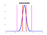
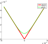
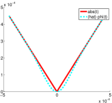
Figure 2: $K_{\sigma}(t)$ and vertical lines at $(-\sigma,\sigma)$ and $(-4\sigma,4\sigma)$ for $\sigma=0.01$. Convolution based approximations to $|t|$.

Let us now compute the limit $\lim_{\sigma\to 0}K_{\sigma}(t)$. For $t=0$, it is immediate that $\lim_{\sigma\to 0}K_{\sigma}(0)=\infty$. For $t\neq 0$, we use l’Hôpital’s rule:

$$\lim_{\sigma\to 0}K_{\sigma}(t)=\lim_{\sigma\to 0}\frac{1}{\sqrt{2\pi\sigma^{2}}}\exp\left(-\frac{t^{2}}{2\sigma^{2}}\right)=\lim_{\gamma\to\infty}\frac{\gamma}{\sqrt{2\pi}\exp\left(\frac{\gamma^{2}t^{2}}{2}\right)}=\frac{1}{\sqrt{2\pi}}\lim_{\gamma\to\infty}\frac{1}{\gamma\,t^{2}\exp\left(\frac{\gamma^{2}t^{2}}{2}\right)}=0,$$

with $\gamma=\frac{1}{\sigma}$. We see that $K_{\sigma}(t)$ behaves like a Dirac delta function $\delta_{0}(x)$ with unit integral over $\mathbb{R}$ and the same pointwise limit. Thus, for small $\sigma>0$, we expect that the absolute value function can be approximated by its convolution with $K_{\sigma}$, i.e.,

$$|t|\approx\phi_{\sigma}(t),\quad\forall\,t\in\mathbb{R},$$ (3.2)

where the function $\phi_{\sigma}:\mathbb{R}\to\mathbb{R}$ is defined as the convolution of $K_{\sigma}$ with the absolute value function:

$$\phi_{\sigma}(t):=(K_{\sigma}*|\cdot|)(t)=\frac{1}{\sqrt{2\pi\sigma^{2}}}\int_{-\infty}^{\infty}|t-s|\exp\left(-\frac{s^{2}}{2\sigma^{2}}\right)\mathrm{d}s,\quad\forall\,t\in\mathbb{R}.$$ (3.3)

We show in Proposition 3.3 below, that the approximation in (3.2) converges in the $L^{1}$ norm (as $\sigma\to 0$). The advantage of using this approximation is that $\phi_{\sigma}$, unlike the absolute value function, is a smooth function.

Before we state the convergence result in Proposition 3.3, we express the convolution integral and its derivative in terms of the well-known error function [1].

Lemma 3.2

For any $\sigma>0$, define $\phi_{\sigma}:\mathbb{R}\to\mathbb{R}$ as in (3.3) Then we have that for all $t\in\mathbb{R}$:

$$\phi_{\sigma}(t)\,= \ t\operatorname{erf}\left(\frac{t}{\sqrt{2}\sigma}\right)+\sqrt{\frac{2}{\pi}}\sigma\exp\left(-\frac{t^{2}}{2\sigma^{2}}\right),$$ (3.4)

$$\frac{\mathrm{d}}{\mathrm{d}t}\,\phi_{\sigma}(t)\,= \ \operatorname{erf}\left(\frac{t}{\sqrt{2}\sigma}\right),$$ (3.5)

where the error function is defined as:

$$\operatorname{erf}(t)=\frac{2}{\sqrt{\pi}}\int_{0}^{t}\exp(-u^{2})\mathrm{d}u\quad\forall\,t\in\mathbb{R}.$$

• $\Box$

The above lemma is proved in [22]. Next, using the fact that the error function $\operatorname{erf}(t)=\frac{2}{\sqrt{\pi}}\int_{0}^{t}\exp(-s^{2})\mathrm{d}s$ satisfies the bounds:

$$\bigl{(}1-\exp(-t^{2})\bigr{)}^{\frac{1}{2}}\leq\operatorname{erf}(t)\leq\bigl{(}1-\exp(-2t^{2})\bigr{)}^{\frac{1}{2}},\quad\forall\,t\geq 0,$$ (3.6)

the following convergence result can be established:

Proposition 3.3

Let $g(t):=|t|$ for all $t\in\mathbb{R}$, and let the function $\phi_{\sigma}:=K_{\sigma}*g$ be defined as in (3.3), for all $\sigma>0$. Then:

$$\lim_{\sigma\to 0}\left\|\phi_{\sigma}-g\right\|_{L^{1}}=0.$$

The proof is again given in [22]. While $g=|\cdot|\not\in L^{1}$ (since $g(t)\to\infty$ as $t\to\infty$), the approximation in the $L^{1}$ norm still holds. It is likely that the convolution approximation converges to $g$ in the $L^{1}$ norm for a variety of non-smooth coercive functions $g$, not just for $g(t)=|t|$.

3.2 Approximation at zero

Note from (3.2) that while the approximation $\phi_{\sigma}(t)=K_{\sigma}*|t|$ is indeed smooth, it is positive on $\mathbb{R}$ and in particular $(K_{\sigma}*|\cdot|)(0)=\sqrt{\frac{2}{\pi}}\sigma>0$, although $(K_{\sigma}*|\cdot|)(0)$ does go to zero as $\sigma\to 0$. To address this, we can use different approximations based on $\phi_{\sigma}(t)$ which are zero at zero. Below, we describe several different alternatives which are possible. The first is formed by subtracting the value at $0$:

$$\tilde{\phi}_{\sigma}(t)=\phi_{\sigma}(t)-\phi_{\sigma}(0)\,=\,t\operatorname{erf}\left(\frac{t}{\sqrt{2}\sigma}\right)+\sqrt{\frac{2}{\pi}}\sigma\exp\left(\frac{-t^{2}}{2\sigma^{2}}\right)-\sqrt{\frac{2}{\pi}}\sigma.$$ (3.7)

An alternative is to use $\tilde{\phi^{(2)}}_{\sigma}(t)=\phi_{\sigma}(t)-\sqrt{\frac{2}{\pi}}\sigma\exp\left(-t^{2}\right)$ where the subtracted term decreases in magnitude as $t$ becomes larger and only has much effect for $t$ close to zero. We could also simply drop the second term of $\phi_{\sigma}(t)$ to get:

$$\hat{\phi}_{\sigma}(t)=\phi_{\sigma}(t)-\sqrt{\frac{2}{\pi}}\sigma\exp\left(\frac{-t^{2}}{2\sigma^{2}}\right)\,=\,t\operatorname{erf}\left(\frac{t}{\sqrt{2}\sigma}\right)$$ (3.8)

which is zero when $t=0$. The behavior is plotted in Figure 2.

3.3 Gradient Computations and Algorithms

We now discuss algorithms for the approximate minimization of (1.1) using the ideas we have developed. In particular, we will focus on the case $l=2$ resulting in the one parameter functional:

$$\tilde{F}_{p}(x)=\|Ax-b\|^{2}_{2}+\lambda\left(\sum_{k=1}^{n}|x_{k}|^{p}\right).$$ (3.9)

We obtain the smooth approximation functional to $\tilde{F}_{p}(x)$:

$$\begin{array}[]{rcl}H_{p,\sigma}(x)&:=&\displaystyle\|Ax-b\|^{2}_{2}+\lambda\left(\sum_{k=1}^{n}\phi_{\sigma}(x_{k})^{p}\right)\\ &=&\displaystyle\|Ax-b\|^{2}_{2}+\lambda\left(\sum_{k=1}^{n}\left(x_{k}\operatorname{erf}\left(\frac{x_{k}}{\sqrt{2}\sigma}\right)+\sqrt{\frac{2}{\pi}}\sigma\exp\left(\frac{-x_{k}^{2}}{2\sigma^{2}}\right)\right)^{p}\right).\end{array}$$ (3.10)

which is of similar form considered in detail in [22]. To compute the gradient of the smooth functional it is enough to consider the function $G_{p}(x)=\displaystyle\sum_{k=1}^{n}\phi_{\sigma}(x_{k})^{p}$. Taking the derivative with respect to $x_{j}$ yields:

$$\frac{\partial}{\partial x_{j}}\phi_{\sigma}(x_{j})^{p}=p\phi_{\sigma}(x_{j})^{p-1}\phi_{\sigma}^{\prime}(x_{j})=p\phi_{\sigma}(x_{j})^{p-1}\operatorname{erf}\left(\frac{x_{j}}{\sqrt{2}\sigma}\right).$$

Taking the second derivative yields:

$$\frac{\partial^{2}}{\partial x_{i}\partial x_{j}}G_{p}(x)=0,$$

when $i\neq j$ and when $i=j$ we have:

$$\frac{\partial^{2}}{\partial x_{j}^{2}}G_{p}(x) = \frac{\partial}{\partial x_{j}}\left\{\left[p\phi_{\sigma}(x_{j})^{p-1}\right]\left[\operatorname{erf}\left(\frac{x_{j}}{\sqrt{2}\sigma}\right)\right]\right\}$$

$$= p(p-1)\phi_{\sigma}(x_{j})^{p-2}\operatorname{erf}^{2}\left(\frac{x_{j}}{\sqrt{2}\sigma}\right)+\left[p\phi_{\sigma}(x_{j})^{p-1}\right]\frac{2}{\sqrt{2}\sqrt{\pi}\sigma}\exp\left(-\frac{x_{j}^{2}}{2\sigma^{2}}\right).$$

The following results follow.

Lemma 3.4

Let $H_{p,\sigma}(x)$ be as defined in (3.10) where $p>0$ and $\sigma>0$. Then the gradient is given by:

$$\nabla{H_{p,\sigma}}(x)=2A^{T}(Ax-b)+\lambda p\bigl{(}\vec{v}(x)\bigr{)},$$ (3.11)

and the Hessian is given by:

$$\nabla^{2}H_{p,\sigma}(x)=2A^{T}A+\lambda p\operatorname{Diag}\bigl{(}\vec{w}(x)\bigr{)},$$ (3.12)

where the functions $\vec{v}:\mathbb{R}^{n}\to\mathbb{R}^{n}$ and $\vec{w}:\mathbb{R}^{n}\to\mathbb{R}^{n}$ are defined for all $x\in\mathbb{R}^{n}$:

$$\vec{v}(x):=\left\{v(x_{j})\right\}_{j=1}^{n}= \ \left\{\phi_{\sigma}(x_{j})^{p-1}\operatorname{erf}\left(\frac{x_{j}}{\sqrt{2}\sigma}\right)\right\}_{j=1}^{n}$$

$$\vec{w}(x):=\left\{w(x_{j})\right\}_{j=1}^{n}= \ \left\{(p-1)\phi_{\sigma}(x_{j})^{p-2}\operatorname{erf}^{2}\left(\frac{x_{j}}{\sqrt{2}\sigma}\right)+\left[\phi_{\sigma}(x_{j})^{p-1}\right]\sqrt{\frac{2}{\pi\sigma^{2}}}\exp\left(-\frac{x_{j}^{2}}{2\sigma^{2}}\right)\right\}_{j=1}^{n}.$$

Given $H_{p,\sigma}(x)\approx\tilde{F}_{p}(x)$ and $\nabla H_{p,\sigma}(x)$, we can apply a number of gradient based methods for the minimization of $H_{p,\sigma}(x)$ (and hence for the approximate minimization of $\tilde{F}_{p}(x)$), which take the following general form:

Pick an initial point $x^{0}$;

for $n=0,1,\ldots$, maxiter do

       Compute search direction $s^{n}$ based on gradient $\nabla H_{p,\sigma}(x^{n})$. ;

       Compute step size parameter $\mu$ via line search. ;

       Update the iterate: $x^{n+1}=x^{n}+\mu s^{n}$. ;

       Check if the termination conditions are met. ;

      

end for

Record final solution: $\bar{x}=x^{n+1}$. ;

Algorithm 2 Generic Gradient Method for finding $\arg\min H_{p,\sigma}(x)$.

Note that in the case of $p<1$, the functional $F_{p}(x)$ is not convex, so such an algorithm may not converge to the global minimum in that case. The generic algorithm above depends on the choice of search direction $s^{n}$, which is based on the gradient, and the line search, which can be performed in several different ways.

3.4 Line Search Techniques

Gradient based algorithms differ based on the choice of search direction vector $s^{n}$ and line search techniques for parameter $\mu$. In this section we describe some suitable line search techniques. Given the current iterate $x^{n}$ and search direction $s^{n}$, we would like to choose $\mu$ so that:

$$H_{p,\sigma}(x^{n+1})=H_{p,\sigma}(x^{n}+\mu s^{n})\leq H_{p,\sigma}(x^{n}),$$

where $\mu>0$ is a scalar which measures how long along the search direction we advance from the previous iterate. Ideally, we would like a strict inequality and the functional value to decrease. Exact line search would solve the single variable minimization problem:

$$\bar{\mu}=\arg\min_{\mu}H_{p,\sigma}(x^{n}+\mu s^{n}).$$

The first order necessary optimality condition (i.e., $\nabla H_{p,\sigma}(x+\mu s)^{T}s=0$) can be used to find a candidate value for $\mu$, but it is not easy to solve the gradient equation. Instead, using the second order Taylor approximation of $n(t):=H_{p,\sigma}(x+ts)$ at any given $x,s\in\mathbb{R}^{n}$, we have that

$$n^{\prime}(t)=n^{\prime}(0)+tn^{\prime\prime}(0)+o(t)\approx n^{\prime}(0)+tn^{\prime\prime}(0)$$ (3.13)

using basic matrix calculus:

$$n^{\prime}(t) = \left(\nabla H_{p,\sigma}(x+ts)\right)^{T}s\implies n^{\prime}(0)=\nabla H_{p,\sigma}(x)^{T}s$$

$$n^{\prime\prime}(t) = \left[\left(\nabla^{2}H_{p,\sigma}(x+ts)\right)^{T}s\right]^{T}s=s^{T}\nabla^{2}H_{p,\sigma}(x+ts)s\implies n^{\prime\prime}(0)=s^{T}\nabla^{2}H_{p,\sigma}(x)s,$$

we get that $n^{\prime}(0)+\mu n^{\prime\prime}(0)=0$ if and only if

$$\mu=-\frac{\nabla H_{p,\sigma}(x)^{T}s}{s^{T}\nabla^{2}H_{p,\sigma}(x)s}.$$ (3.14)

An alternative approach is to use a backtracking line search to get a step size $\mu$ that satisfies one or two of the Wolfe conditions [12]. This update scheme can be slow since several evaluations of $H_{p,\sigma}(x)$ may be necessary, which are relatively expensive when the dimension $n$ is large. The Wolfe condition scheme also necessitates the choice of further parameters.

3.5 Nonlinear Conjugate Gradient Algorithm

We now present the conjugate gradient scheme in Algorithm 3, which can be used for sparsity constrained regularization. In the basic (steepest) descent algorithm, we simply take the negative of the gradient as the search direction. For nonlinear conjugate gradient methods, several different search direction updates are possible. We find that the Polak-Ribière scheme often offers good performance [14, 15, 17]. In this scheme, we set the initial search direction $s^{0}$ to the negative gradient, as in steepest descent, but then do a more complicated update involving the gradient at the current and previous steps:

$$\beta^{n+1} = \max\left\{\frac{\nabla H_{p,\sigma_{n}}(x^{n+1})^{T}\left(\nabla H_{p,\sigma_{n}}(x^{n+1})-\nabla H_{p,\sigma_{n}}(x^{n})\right)}{\nabla H_{p,\sigma_{n}}(x^{n})^{T}\nabla H_{p,\sigma_{n}}(x^{n})},0\right\},$$

$$s^{n+1} = -\nabla H_{p,\sigma_{n}}(x^{n+1})+\beta^{n+1}s^{n}.$$

One extra step we introduce in Algorithm 3 is a thresholding which sets small components to zero. That is, at the end of each iteration, we retain only a portion of the largest coefficients. This is necessary, as otherwise the solution we recover will contain many small noisy components and will not be sparse. In our numerical experiments, we found that soft thresholding works well when $p=1$ and that hard thresholding works better when $p<1$. The component-wise soft and hard thresholding functions with parameter $\lambda>0$ are given by:

$$\left(\mathbb{S}_{\lambda}(x)\right)_{k}=\left\{\begin{array}[]{ll}x_{k}-\lambda,&\hbox{$x_{k}>\lambda$}\\ 0,&\hbox{$-\lambda\leq x_{k}\leq\lambda$;}\\ x_{k}+\lambda,&\hbox{$x_{k}<-\lambda$ }\\ \end{array}\right.\quad\left(\mathbb{H}_{\lambda}(x)\right)_{k}=\left\{\begin{array}[]{ll}x_{k},&\hbox{$|x_{k}|>\lambda$}\\ 0,&\hbox{$-\lambda\leq x_{k}\leq\lambda$}\end{array},\right.\quad\forall\,x\in\mathbb{R}^{n}.$$ (3.15)

For $p=1$, an alternative to thresholding at each iteration at $\lambda$ is to use the optimality condition of the $F_{1}(x)$ functional [5]. After each iteration (or after a block of iterations), we can evaluate the vector

$$v^{n}=A^{T}(b-Ax^{n}).$$ (3.16)

We then set the components (indexed by $k$) of the current solution vector $x^{n}$ to zero for indices $k$ for which $|v^{n}_{k}|\leq\frac{\lambda}{2}$.

Note that after each iteration, we also vary the parameter $\sigma$ in the approximating function to the absolute value $\phi_{\sigma}$, starting with $\sigma$ relatively far from zero at the first iteration and decreasing towards $0$ as we approach the iteration limit. The decrease can be controlled by a parameter $\alpha\in(0,1)$ so that $\sigma_{n+1}=\alpha\sigma_{n}$. The choice $\alpha=0.8$ worked well in our experiments. Comments on the computational cost relative to the FISTA algorithm are discussed in [22], where it is shown that the most expensive matrix-vector multiplication operations are present in both algorithms. On the other hand, the overhead with using CG iterations is significant and each iteration does take more time than that of a thresholding method. The algorithm is designed to be run for a small number of iterations.

In Algorithm 3, we present a nonlinear Polak-Ribière conjugate gradient scheme to approximately minimize $\tilde{F}_{p}$ [14, 15, 17]. The function $\mathtt{Threshold}(\cdot,\tau)$ in the algorithms which enforces sparsity refers to either one of the two thresholding functions defined in (3.15) or to the strategy using the $v^{n}$ vector in (3.16). The update rule for $\sigma$ can be varied. In particular, it can again be tied to the distance between two successive iterates (e.g. $\sigma_{n+1}=\min\left(\sigma_{0},\alpha*\|x^{n+1}-x^{n}\|\right)$), although care must be taken not to make $\sigma$ too small, which has the effect of introducing a nearly sharp corner. Another possibility, given access to both gradient and Hessian, is to use a higher order root finding method, such as Newton’s method [12] as discussed in [22].

Input : An $m\times n$ matrix $A$, an initial guess $n\times 1$ vector $x^{0}$, a parameter $\tau<\|A^{T}b\|_{\infty}$, a parameter $p\in[1,2]$, a parameter $\sigma_{0}>0$, a parameter $0<\alpha<1$, the maximum number of iterations $N$, and a routine to evaluate the gradient $\nabla H_{p,\sigma}(x)$ (and possibly the Hessian $\nabla^{2}H_{p,\sigma}(x)$ depending on choice of line search method).

Output : A vector $\bar{x}$, close to either the global or local minimum of $\tilde{F}_{p}(x)$, depending on choice of $p$.

$s^{0}=-\nabla H_{p,\sigma_{0}}(x^{0})$ ;

for $n=0,1,\ldots$,N do

       use line search to find $\mu>0$;

       $x^{n+1}=\mathtt{Threshold}(x^{n}+\mu s^{n},\tau)$ ;

       $\beta^{n+1}=\max\left\{\frac{\nabla H_{p,\sigma_{n}}(x^{n+1})^{T}(\nabla H_{p,\sigma_{n}}(x^{n+1})-\nabla H_{p,\sigma_{n}}(x^{n}))}{\nabla H_{p,\sigma_{n}}(x^{n})^{T}\nabla H_{p,\sigma_{n}}(x^{n})},0\right\}$ ;

       $s^{n+1}=-\nabla H_{p,\sigma_{n}}(x^{n+1})+\beta^{n+1}s^{n}$ ;

       $\sigma_{n+1}=\alpha\sigma_{n}$ ;

      

end for

$\bar{x}=x^{n+1}$;

Algorithm 3 CONV CG Algorithm

3.6 Application to generalized residual penalty and wavelet representations

First, we comment on the application of the CONV CG method to (1.1). In this case, the change of variables $y=Ax-b$ gives the constrained minimization problem:

$$\min_{y,x}\left\{\|y\|_{l}^{l}+\lambda\|x\|_{p}^{p}\right\}\quad\mbox{s.t.}\quad y=Ax-b.$$

This can be accomplished via e.g. an alternative variable minimization scheme combined with the Lagrange multiplier method, in which case we get the minimization problem:

$$\min_{y,x,s}\left\{\|y\|_{l}^{l}+\lambda\|x\|_{p}^{p}+s^{T}(Ax-b-y)\right\}$$

where $s$ is a vector of Lagrange multipliers. We can use the alternate minimization method to minimize with respect to each variable in a loop. Let us now assume that $l\in(1,2)$ and that all $y_{i}\neq 0$. In this case, minimizing with respect to $y$ by setting the gradient to zero:

$$l\left\{y_{i}^{l-1}\right\}_{i=1}^{m}-s=0.$$

Next, for minimizing with respect to $x$, we will use the convolution based approximation, since some entries of $x$ can indeed be zero. We get, for each component:

$$\frac{\partial}{\partial x_{i}}\left[\displaystyle\sum_{k=1}^{n}\phi_{\sigma}(x_{k})^{p}+s^{T}Ax\right]=p\phi_{\sigma}(x_{i})^{p-1}\operatorname{erf}\left(\frac{x_{i}}{\sqrt{2}\sigma}\right)+\left[A^{T}s\right]_{i}=0,$$

which is a nonlinear system to be solved for each component $i$. (The derivative with respect to $s$ simply yields $Ax-b-y=0$). A more efficient approach is to again assume that all $r_{i}=(Ax-b)_{i}\neq 0$ and utilize the same result from [16], yielding in place of (3.11), the gradient:

$$\nabla{H_{l,p,\sigma}}(x)=A^{T}R(Ax-b)+\lambda p\bigl{(}\vec{v}(x)\bigr{)},$$

with $R=\operatorname{diag}(l|r_{i}(x)|^{l-2})$ as before. In practice, $R$ would be iteration dependent, as in the IRLS scheme. The Hessian can also be computed using the results from (2.11), taking care of the fact that $R$ depends on $x$.

Secondly, we comment on the application of our methods in a transformed basis. This is useful when for example, we are dealing with images, which are not outright sparse, but can indeed be efficiently represented by the use of wavelet transforms. In this case, we would like to apply the sparse penalty to $w=Wx$, where $W$ is the wavelet transformed matrix. While $w$ may not be sparse, we can remove many of the smaller magnitude coefficients of $w$, such that the resulting vector $\tilde{w}$ satisfies, $W^{-1}\tilde{w}\approx x$. We can consider the minimization of the functional:

$$\|Ax-b\|_{l}^{l}+\lambda\|w\|_{p}^{p},$$

which with the substitution $x=W^{-1}w$ becomes a function of a single variable $w$. Both algorithms can then be applied to this formulation, using the matrix $AW^{-1}$ (in practice, we only need to be able to apply the transform and not to form the $W^{-1}$ matrix explicitly). For values of $p$ closer to $1$ this formulation often yields better results then the inversion in the default basis for signals which are approximately sparse under $W$ in the above sense. For image deconvolution and other formulations, we can also introduce a smoothing term into the regularization. For instance, we can minimize:

$$\|Ax-b\|_{2}^{2}+\lambda_{1}\|w\|_{p}^{p}+\lambda_{2}\|Lx\|_{2}^{2},$$

with $L$ a tridiagonal “Laplacian” kind of matrix. We can again plug in $x=W^{-1}w$ or extend this using the Lagrange multiplier formulation, obtaining the optimization problem:

$$\min_{x,w,s}P(x,w,s)=\min_{x,w,s}\left\{\|Ax-b\|_{2}^{2}+\lambda_{1}\|w\|_{p}^{p}+\lambda_{2}\|Lx\|_{2}^{2}+s^{T}(Wx-w)\right\}.$$

The minimization with respect to $s$ (yielding $Wx=w$) and with respect to $x$ yielding:

$$2A^{T}(Ax-b)+2\lambda_{2}L^{T}Lx+W^{T}s=0,$$

to be solved for $s$ are straightforward. On the other hand, the minimization with respect to $w$ (making use of the convolution gradient result), produces again a nonlinear system. For instance, taking $p=1$, $\frac{\partial P}{\partial w}=0$ gives:

$$(AW^{-1})^{T}(AW^{-1}w-b)+\lambda_{1}\operatorname{erf}\left(\frac{w_{j}}{\sqrt{2}\sigma}\right)|_{j=1}^{n}-s=0$$

which is a nonlinear system for each $j$. When the dimensionality ($n$) is large, solving such systems at each iteration is very expensive. We aim to investigate more efficient formulations for such problems (e.g. deconvolution) as part of upcoming work.

4 Numerical Experiments

First, we aim to carry out a synthetic (2–D) seismic tomography experiment to quantify the usefulness of the functional (1.1) which we consider. In particular, we will use our IRLS CG algorithm to approximately minimize this functional with different choices of $l$.

We take a linear, tomographic system $Ax=b$, where the model parameters, $x$, are shear-wave velocity perturbations (dlnVs) and the model parametrization consists of $n=1024$ square-pixels (see Fig. 3(a)). In the framework of ray theory, data represent onset time-residuals of direct S waves, whose ray paths are straight lines from one black dot to another (see Fig. 3(a)). The total number of data that we consider is $m=400$ (i.e., $m\ll n$). Each element $A_{ij}$ of the sensitivity matrix represents the length of the $i$-th ray inside the $j$-th pixel.

For a given input, true model, $x^{\text{true}}$, the noisy (outlier-free) data set is computed as: $b\leftarrow Ax^{\text{true}}+n$, for realistic, random noise $n$ (see Fig. 3(b)). Here, we consider the ‘checkerboard’ true model displayed in Fig. 3(c). The damped least-squares (DLS) model solution, obtained from LSQR inversion of the (outlier-free) data set $b$ is shown in Fig. 3(d).

Let us consider the previous (outlier-free) data set, $b$, to which we add some ‘outlier’ time-residuals, $n^{\text{outliers}}$, that is: $b^{\text{outliers}}\leftarrow b+n^{\text{outliers}}$ (see Fig. 3(e)). The DLS solution, obtained from LSQR inversion of the outlier data set, $b^{\text{outliers}}$, is then displayed in Fig. 3(f). Moreover, the corresponding solutions obtained from the same outlier data set, $b^{\text{outliers}}$, using our IRLS CG scheme with $l=1.0$ and $l=1.8$ are shown in Figs. 3(g) and (h), respectively.

We see that: 1) DLS is fine for outlier-free data, but not so for outlier data; 2) Our IRLS CG algorithm proves to give better results than DLS for outlier data – when using $l$ values close to unity. That is, keeping $l$ close to $2$ gives a big effect in the solution, due to the inclusion of outlier time-residuals. On the other hand, $l$ closer to $1$ imposes a bigger penalty on the outlier residual terms and produces a solution closer to the (DLS) case of outlier-free data.

As this synthetically constructed example shows, the ability to control the $l$ parameter in the functional allows to mitigate the effects of outlier residuals in the data. As a remark, automatically removing outliers (e.g., related to mis-picking of seismic phases) in massive data sets may be a very difficult task, so that most data sets in (geo)physics shall come with outliers.

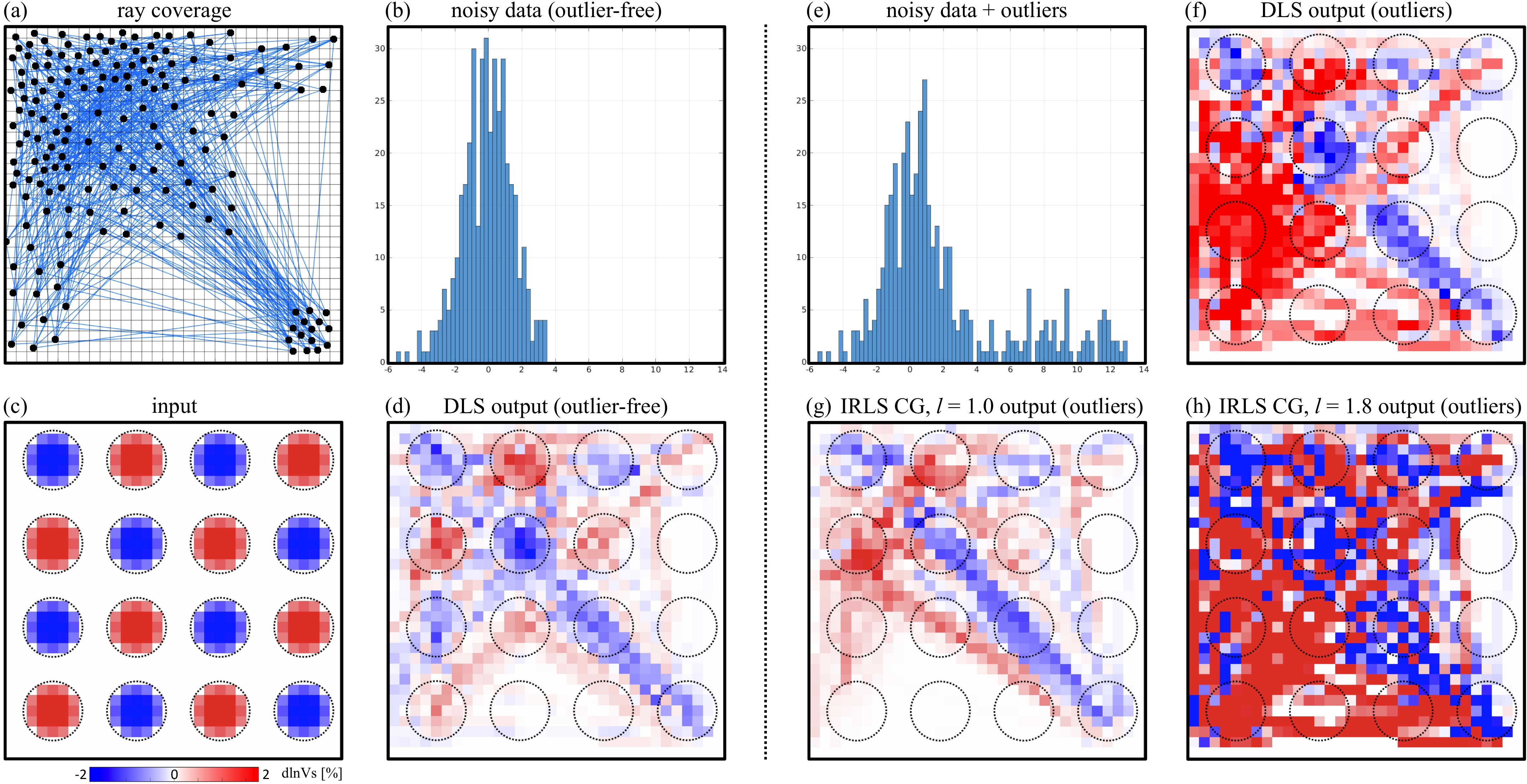
Figure 3: Tomographic experiment – (a) Ray coverage and model parametrization (square-pixels); (b) Histogram of the outlier-free data set, $b$; (c) Input model, $x^{\text{true}}$; (d) DLS output solution for (univariant) data set $b$; (e) Histogram of the outlier data set, $b^{\text{outlier}}$; (f) IRLS CG output solution, with $l=1.0$, for data set $b^{\text{outlier}}$; (g) IRLS CG output solution, with $l=1.8$, for data set $b^{\text{outlier}}$.

In our second experiment, we compare the power of the different methods in decreasing the cost functional we are trying to minimize, per iteration. We run each algorithm along an L-curve, decreasing the regularization parameter $\lambda$ and reusing the previous solution as the initial guess at the next $\lambda$. Typically, we stop the procedure, either when the noise level is approximately matched (e.g. when $\|Ax_{\lambda}-b\|_{2}\approx\|\text{noise}\|_{2}$, if the noise norm value is known) or at some optimal trade-off point along the curve. This point is often estimated by taking the region of maximum curvature between the terms $\log\|Ax_{\lambda}-b\|_{l}$ and $\|x_{\lambda}\|_{p}$ (or of $\|w_{\lambda}\|_{p}$, if a transformed basis is used).

In Figure 4, we compare the cost reduction power of the different algorithms along the L curve. To compare with FISTA, we set $l=2,p=1$. We use $1000\times 1000$ test matrices with two different rates of logarithmic singular value decay ($logspace(0,-0.5,k)$ and $logspace(0,-2.5,k)$ with $k=\min(m,n)=1000$ in Octave notation). At each value of $\lambda$ we use $3$ iterations. From the figure, we observe that each iteration of IRLS CG and CONV CG is more powerful than that of a thresholding scheme, in the sense that it results in greater functional reduction along the initial parts of the L curve. In particular, while each iteration of the CONV CG is more expensive than that of other schemes, just a few iterations of the method would be enough to yield a good warm start solution, or build an estimate of the shape of the L curve. As can be observed in Figure 4, the effect becomes more pronounced as the matrix condition worsens.

In Figure 5, we present the results of a wavelet based reconstruction experiment using a CDF97 wavelet basis and a simple multi-scale model. In this experiment, a complete L curve is constructed. In the first row, we illustrate the L curve based reconstruction with the CONV CG algorithm using a well conditioned matrix $A$. Using $5$ iterations at each value of $\lambda$ (on a logarithmic scale of $50$ values from $\frac{\|(AW^{-1})^{T}b\|_{\infty}}{1.2}$ to $\frac{\|(AW^{-1})^{T}b\|_{\infty}}{10^{6}}$), we run the CONV CG scheme to minimize $\|Ax-b\|_{2}^{2}+\lambda\|w\|_{1}$ (applying the sparsity constraint in the Wavelet basis) and reuse the solution as the initial guess at each next iteration. We reconstruct the solution in the original basis by applying the inverse transform. We plot the tradeoff curve of the quantities $\log\|Ax_{\lambda}-b\|_{2}$ and $\log\|w_{\lambda}\|_{1}$ and a plot of the curvature of these quantities as a function of $\lambda$, estimated using finite differences. As we can see from the error vs parameter plot, the reconstruction error drops as we approach the point of maximum curvature along the L curve. In the subsequent two rows, we compare the performance of FISTA and CG schemes for such a reconstruction, using $5$ iterations at each value of $\lambda$. Now however, we use a worse conditioned matrix with logspaced singular values ($logspace(0,-1.5,k)$), for which the problem is more challenging. We see that the CONV CG algorithm produces lower percent errors and hence, a closer reconstruction for the same number of iterations used. This example illustrates the utility of the CONV CG scheme for efficient model reconstruction and for parameter (optimal $\lambda$ value) estimation.

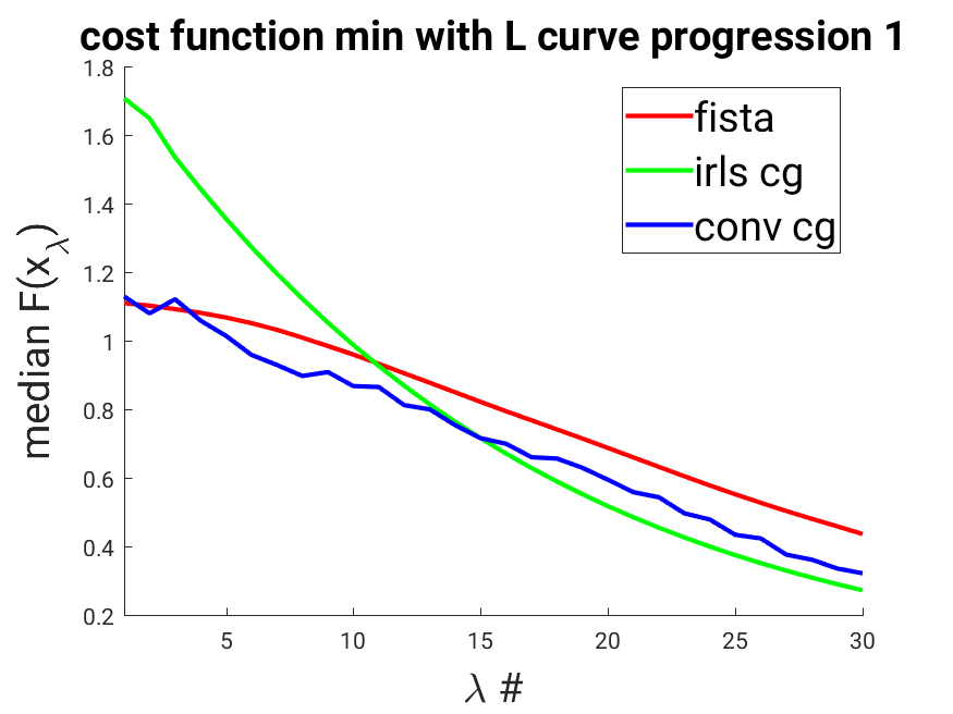
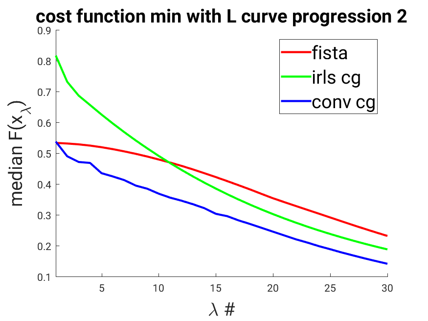
Figure 4: Comparison of cost function reduction (over 10 trials) along L-curve progression by FISTA, IRLS CG, and CONV CG schemes over better and worse conditioned matrices.

.

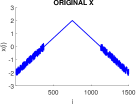
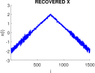
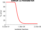
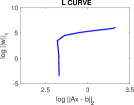
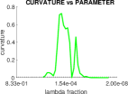
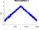
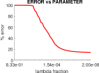
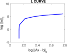
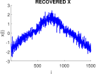
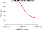
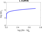
Figure 5: Comparison of L-curve construction by CONV CG and FISTA schemes. Row 1: L curve illustration with a well conditioned matrix. Row 2: CONV CG solution for the worse conditioned matrix. Row 3: FISTA solution for the worse conditoned matrix.

5 Conclusions

In this paper we present two algorithms based on the CG algorithm, useful in a variety of inverse problems. One merit in the methods is in the ability to approximately minimize a more general functional, controlled via two parameters $l$ and $p$. The functional is useful in a variety of applications, with the $l$ parameter controlling the behavior of the residual term (and e.g. the influence of data value variations and outliers on the solution) and with $p$ controlling the type of penalty on the components of the solution vector (allowing either a minimum norm based penalty or a sparsity promoting penalty term). The other merit is in the increased power of the methods per iteration, compared to e.g. thresholding based methods, via the use of the heavily researched CG algorithm (and its many possible variants) at each iteration. This allows for the construction of approximate regularized solutions as defined by the minimization problem in (1.1), at fewer iterations.

References

- [1] Milton Abramowitz and Irene A. Stegun, editors. Handbook of mathematical functions with formulas, graphs, and mathematical tables. A Wiley-Interscience Publication. John Wiley & Sons, Inc., New York; National Bureau of Standards, Washington, DC, 1984.
- [2] Amir Beck and Marc Teboulle. A fast iterative shrinkage-thresholding algorithm for linear inverse problems. SIAM J. Imaging Sci., 2(1):183–202, 2009.
- [3] Demba Ba Behtash Babadi, Patrick L Purdon, and Emery N Brown. Convergence and stability of a class of iteratively re-weighted least squares algorithms for sparse signal recovery in the presence of noise. IEEE transactions on signal processing: a publication of the IEEE Signal Processing Society, 62(1):183, 2013.
- [4] Rick Chartrand. Fast algorithms for nonconvex compressive sensing: Mri reconstruction from very few data. In Int. Symp. Biomedical Imaing, 2009.
- [5] I. Daubechies, M. Defrise, and C. De Mol. An iterative thresholding algorithm for linear inverse problems with a sparsity constraint. Communications on Pure and Applied Mathematics, 57(11):1413–1457, 2004.
- [6] Ingrid Daubechies, Ronald DeVore, Massimo Fornasier, and C Sinan Güntürk. Iteratively reweighted least squares minimization for sparse recovery. Communications on Pure and Applied Mathematics, 63(1):1–38, 2010.
- [7] Zdzisław Denkowski, Stanisław Migórski, and Nikolas S. Papageorgiou. An introduction to nonlinear analysis: theory. Kluwer Academic Publishers, Boston, MA, 2003.
- [8] Heinz W. Engl, Martin Hanke, and A. Neubauer. Regularization of Inverse Problems. Springer, 2000.
- [9] Massimo Fornasier, Steffen Peter, Holger Rauhut, and Stephan Worm. Conjugate gradient acceleration of iteratively re-weighted least squares methods. Computational Optimization and Applications, 65(1):205–259, 2016.
- [10] Per Christian Hansen. The L-curve and its use in the numerical treatment of inverse problems. IMM, Department of Mathematical Modelling, Technical Universityof Denmark, 1999.
- [11] L. Landweber. An iteration formula for Fredholm integral equations of the first kind. Amer. J. Math., 73:615–624, 1951.
- [12] Jorge Nocedal and Stephen J. Wright. Numerical optimization. Springer Series in Operations Research and Financial Engineering. Springer, New York, second edition, 2006.
- [13] Christopher C Paige and Michael A Saunders. Lsqr: An algorithm for sparse linear equations and sparse least squares. ACM transactions on mathematical software, 8(1):43–71, 1982.
- [14] E. Polak and G. Ribière. Note sur la convergence de méthodes de directions conjuguées. Rev. Française Informat. Recherche Opérationnelle, 3(16):35–43, 1969.
- [15] B.T. Polyak. The conjugate gradient method in extremal problems. {USSR} Computational Mathematics and Mathematical Physics, 9(4):94 – 112, 1969.
- [16] John A Scales, Adam Gersztenkorn, and Sven Treitel. Fast lp solution of large, sparse, linear systems: Application to seismic travel time tomography. Journal of Computational Physics, 75(2):314–333, 1988.
- [17] J. R. Shewchuk. An Introduction to the Conjugate Gradient Method Without the Agonizing Pain. Technical report, Pittsburgh, PA, USA, 1994.
- [18] N. Z. Shor, Krzysztof C. Kiwiel, and Andrzej Ruszcayǹski. Minimization Methods for Non-differentiable Functions. Springer-Verlag New York, Inc., New York, NY, USA, 1985.
- [19] Albert Tarantola and Bernard Valette. Inverse Problems = Quest for Information. Journal of Geophysics, 50:159–170, 1982.
- [20] Sergey Voronin. Regularization of linear systems with sparsity constraints with applications to large scale inverse problems. PhD thesis, 2012.
- [21] Sergey Voronin and Ingrid Daubechies. An iteratively reweighted least squares algorithm for sparse regularization. arXiv preprint arXiv:1511.08970, 2015.
- [22] Sergey Voronin, Gorkem Ozkaya, and Davis Yoshida. Convolution based smooth approximations to the absolute value function with application to non-smooth regularization. arXiv preprint arXiv:1408.6795, 2014.