Qubit absorption refrigerator at strong coupling

Abstract

We demonstrate that a quantum absorption refrigerator can be realized from the smallest quantum system, a qubit, by coupling it in a non-additive (strong) manner to three heat baths. This function is un-attainable for the qubit model under the weak system-bath coupling limit, when the dissipation is additive. In an optimal design, the reservoirs are engineered and characterized by a single frequency component. We obtain then closed expressions for the cooling window and refrigeration efficiency, as well as bounds for the maximal cooling efficiency and the efficiency at maximal power. Our results agree with macroscopic designs and with three-level models for quantum absorption refrigerators, which are based on the weak system-bath coupling assumption. Beyond the optimal limit, we show with analytical calculations and numerical simulations that the cooling efficiency varies in a non-universal manner with model parameters. Our work demonstrates that strongly-coupled quantum machines can exhibit function that is un-attainable under the weak system-bath coupling assumption.

I Introduction

An autonomous absorption refrigerator transfers thermal energy from a cold ($c$) bath to a hot ($h$) bath without input power, by utilizing heat from an additional heat bath, a so-called work ($w$) reservoir. Classical, large-scale absorption refrigerators were realized in the 19th century AR19 , playing an important role in the development of the theory of irreversible thermodynamics. Proposals for quantum, nanoscale analogues of such machines aspire to establish the theory of thermodynamics from quantum principles review1 ; kos13 ; reviewARPC14 .

Quantum thermodynamical machines differ from their classical counterparts in two central aspects. First, their performance relies on quantum phenomena such as the discreteness of the energy spectrum of the working medium and quantum statistics. Moreover, nontrivial quantum effects such as quantum coherence in the system, scully0 ; scully1 ; scully2 ; HuberC ; Anders or in the bath Lutz ; Alicki15 ; Bijay-squeeze ; manzano2016a , quantum correlations Huber ; Alickientang , non-locality, measurement Kur ; Alicki13 , and quantum driving and control jacobs2009a ; strasberg2013b , may offer new principles for thermal machines. Beyond quantum resources, a second, fundamental aspect of nanoscale heat machines is that they may operate beyond the weak system-bath coupling limit DavidS ; Kosloff ; Cao ; Gernot ; Eisert-strong ; Jarzynski ; esposito17 ; Nazir ; Celardo . Classical-macroscopic thermodynamics is a weak-coupling theory; the impact of the system-bath interface is small relative to the bulk behavior. In contrast, small systems can strongly couple to their surroundings, in the sense that the interaction energy between the system and the bath becomes comparable to frequencies of the isolated system.

The goal of the present paper is to demonstrate that strongly-coupled system-bath quantum machines can exhibit function that is un-attainable under the weak coupling assumption. We do so by analyzing additive and non-additive system-bath interaction models, i.e., where the generator may or may not be additively decomposed into individual generators from the connected reservoirs. In the additive case, the system (working medium) separately-independently exchanges energy with the hot, cold and work reservoirs. In the non-additive model, the reservoirs inseparably interact with the system, thus acting in a concerted-cooperative manner.

Specifically, we show that a two-level system (TLS) cannot operate as an autonomous quantum absorption refrigerator (QAR) under the weak system-bath coupling approximation with additive dissipators. However, the same system does function as a QAR once it is allowed to couple to its surrounding reservoirs in a non-additive manner—representing strong coupling. Moreover, the qubit QAR can be optimized to perform at the maximal Carnot efficiency, and its performance is compatible with previous designs using three-level models, which were constrained to operate under Lindblad dynamics with additive dissipators jose13 ; joseSR ; jose14 . The smallest possible QAR described here relies on quantum principles and strong system-bath coupling effects. These unique aspects are inherent to nanoscale devices.

This work is organized as follows: We first introduce our model, showing that a QAR mode is impossible in the additive case (Sec. II.1), and afterwards present the non-additive model (Sec. II.2), for which we present the basic definitions of energy currents for two and three reservoirs. Next, we present analytical results for the non-additive model, first on the cooling window and efficiency for specific spectral densities in Sec. III.1 and then on the cooling efficiency at maximum power in Sec. III.2. For rectangular spectral densities we confirm these results by numerical simulations in Sec. IV. Finally, we show explicitly how such a non-additive dissipator may arise in the strong-coupling limit in Sec. V.

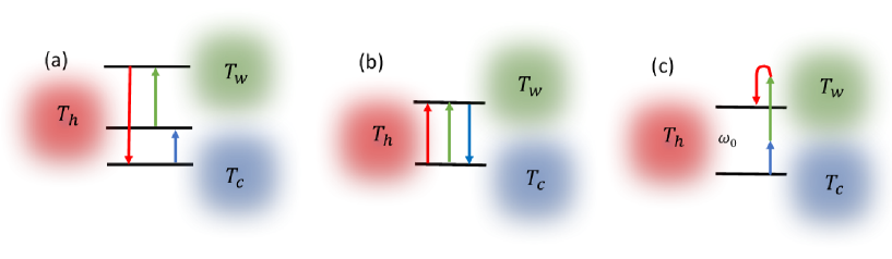
Figure 1: (a) A three-level quantum system, with each transition thermalized separately with respect to an independent bath, hot (h), cold (c) and work (w). This model, which can operate as an absorption refrigerator reviewARPC14 ; joseSR , is not examined in the present work. (b) A two-level system with an additive interaction model, Eq.  (1). This system cannot act as a QAR under the weak-coupling approximation. (c) A two-level system with an inseparable interaction model to the baths, Eq. (4). The concerted action of the baths is represented by the arrows, acting together to e.g., excite the qubit. This model is examined in the present work. When optimized, it performs as a QAR under conditions analogous to the three-level QAR of panel (a).

II Model

A common design of an autonomous QAR consists of a three-level quantum system and three independent thermal reservoirs reviewARPC14 . Each transition between a pair of levels is weakly coupled to only one of the three heat baths, $c$, $h$ and $w$, where $T_{w}>T_{h}>T_{c}$, see Fig. 1a. In the steady state limit, the (ultra-hot) work bath provides energy to the system. This allows the extraction of energy from the cold bath, to be dumped into the hot reservoir. The opposite heating process, from the hot bath to the cold, takes place as well, but it can be minimized by manipulating the frequencies of the system. The three-level QAR was discussed in details in several recent studies, see e.g. Refs. reviewARPC14 ; joseSR ; jose14 . It is designed to perform optimally under the weak coupling approximation, when each bath individually couples to a different transition. Quantum coherent and strong coupling effects are expected to reduce the cooling performance of a three-level QAR.

In this paper we focus on a QAR made of a two-level system coupled to three independent thermal baths. When the baths couple to the qubit in an additive manner (Fig. 1b) we prove next that it is impossible to cool down the cold bath when the system-bath coupling is weak. By allowing for cooperative system-bath interaction between the qubit and the reservoirs (Fig. 1c), we are able to receive a cooling condition, as well as derive bounds for the maximal efficiency of the QAR and its maximal power efficiency.

II.1 Un-attainability of cooling for an additive dissipation model

The additive model comprises a two-level system (spin, qubit) and three independent thermal reservoirs $\nu=c,h,w$, $T_{w}>T_{h}>T_{c}$, $\beta_{\nu}=1/T_{\nu}$ with $k_{B}=1$. The generic Hamiltonian is written as

$$\hat{H}=\frac{\omega_{0}}{2}\hat{\sigma}_{z}+\sum_{\nu}\hat{H}_{B,\nu}+\frac{\hat{\sigma}_{x}}{2}\otimes\left(\hat{A}_{c}+\hat{A}_{h}+\hat{A}_{w}\right).$$ (1)

Here, $\hat{\sigma}$ are the Pauli spin matrices. $\hat{H}_{B,\nu}$ is the Hamiltonian of the $\nu$-th reservoir. It includes, for example, a collection of harmonic oscillators of frequencies $\omega_{j,\nu}$, $\hat{H}_{B,\nu}=\sum_{j}\omega_{j,\nu}\hat{b}_{j,\nu}^{\dagger}\hat{b}_{j,\nu}$ with $b^{\dagger}$ ($\hat{b}$) as bosonic creation (annihilation) operators. The bath operator $\hat{A}_{\nu}$ is assumed to be hermitian. It couples the bath $\nu$ to the spin, where e.g. $\hat{A}_{\nu}=\sum_{j}\lambda_{j,\nu}\left(\hat{b}_{j,\nu}^{\dagger}+\hat{b}_{j,\nu}\right)$ with coupling strength $\lambda_{j,\nu}$.

Assuming a factorized-product initial state, $\langle\hat{A}_{\nu}\rangle=0$ with the average performed over the initial-canonical state of the bath, weak system-bath coupling and Markovian dynamics, we obtain a second order perturbative, Markovian quantum master equation Breuer . This standard Born-Markov scheme results in the stationary populations of the excited and ground state, respectively,

$$p_{e}=\frac{k_{u}}{k_{d}+k_{u}},\,\,\,\,p_{g}=\frac{k_{d}}{k_{d}+k_{u}},$$ (2)

with $k_{d,u}=\sum_{\nu}k_{d,u}^{(\nu)}$. The decay ($d$) and excitation ($u$) rate constants $k_{d,u}^{(\nu)}$, induced by the $\nu$-th bath, depend on the details of the model. The detailed balance relation dictates local thermal equilibrium, $k_{u}^{(\nu)}/k_{d}^{(\nu)}=e^{-\beta_{\nu}\omega_{0}}$. The energy current, defined positive when flowing towards the qubit, can be similarly derived from the Born-Markov approximation, and it is given by $J_{c}=-\omega_{0}\left(k_{d}^{(c)}p_{e}-k_{u}^{(c)}p_{g}\right)$ segal-nitzan ; segal-master ; segal-nicolin ; nazim . Substituting the steady state population (2) we obtain

$$J_{c}=-\frac{\omega_{0}}{k_{d}+k_{u}}\left[k_{d}^{(c)}k_{d}^{(h)}\left(\frac{k_{u}^{(h)}}{k_{d}^{(h)}}-\frac{k_{u}^{(c)}}{k_{d}^{(c)}}\right)+k_{d}^{(c)}k_{d}^{(w)}\left(\frac{k_{u}^{(w)}}{k_{d}^{(w)}}-\frac{k_{u}^{(c)}}{k_{d}^{(c)}}\right)\right].$$ (3)

Using the detailed-balance relation and the fact that $(e^{-\beta_{h,w}\omega_{0}}-e^{-\beta_{c}\omega_{0}})>0$, we conclude that $J_{c}<0$ irrespective of the details of the model. Equation (3) reveals that under the additive model at weak coupling, every two reservoirs exchange energy independently. The prefactor in the denominator, $k_{d}+k_{u}$, which includes contributions from the three baths, only renormalizes the current. Since every two baths separately communicate, thermal energy always flows towards the colder bath, and a chiller performance is un-attainable.

It should be pointed out that time-dependent, driven or stochastic models can realize refrigeration based on a qubit as a working medium even at weak coupling, see e.g. Refs. kos0 ; kos1 ; kos2 ; kos3 ; segal1 ; segal2 ; segal3 ; kur13 . These type of driven machines are beyond the scope of our work.

II.2 Non-additive (strong) coupling model

It is evident that to realize a QAR with a qubit as the working substance, we must go beyond the model Hamiltonian (1), or the weak-coupling approximation. Our starting point is a revised Hamiltonian with a built-in strong-coupling characteristic, a non-additive system-bath interaction operator,

$$\hat{H}=\frac{\omega_{0}}{2}\hat{\sigma}_{z}+\sum_{\nu}\hat{H}_{B,\nu}+\gamma\frac{\hat{\sigma}_{x}}{2}\otimes\left(\hat{B}_{c}\otimes\hat{B}_{h}\otimes\hat{B}_{w}\right).$$ (4)

Here, $\hat{B}_{\nu}$ are bath operators, assumed to be hermitian, and $\gamma$ is an energy parameter characterizing the interaction energy. The non-additivity of our model is assumed to arise from a more fundamental Hamiltonian with strong interactions between the quantum system and individual reservoirs segal-nitzan ; segal-master ; segal-nicolin , see Sec. V. Non-additive models such as (4) can be also accomplished by engineering many-body Hamiltonians based on e.g. resonant conditions and selection rules.

We emphasize that our model (4) differs in a fundamental way from the QAR model analyzed theoretically in e.g. Refs. Levy12 ; reviewARPC14 ; plenio and realized experimentally in a recent study QAR-exp . In Refs. Levy12 ; reviewARPC14 ; plenio ; QAR-exp , the working medium includes three degrees of freedom such as three harmonic oscillators, which interact via a three-body interaction term. Each oscillator is independently coupled to its own thermal bath, taken into account by introducing additive Lindblad dissipators into the time evolution equation. In contrast, in our model (4) the quantum system is as simple as it can be, a qubit. Nonlinearity is encoded into the model by assuming a non-additive interaction Hamiltonian with the three baths. This inseparability prevents us from arriving at standard perturbative quantum master equations with additive dissipators (standard multi-terminal Lindblad or Redfield).

Back to Eq. (4), we study the system’s dynamics assuming a fully factorized initial state by using the Born-Markov approximation with the perturbative parameter $\gamma$. While this is analogous to a weak coupling treatment, we emphasize again that the model is defined with an inherent strong-coupling feature, the non-additivity of the interaction.

II.2.1 Two-bath model

Equations of motion for the spin polarization, as well as the energy current, were derived in Refs. segal-nicolin ; hava for the model (4) with two baths (hot and cold). The derivation relies on the assumption $\langle\hat{B}_{\nu}\rangle=0$, which could be satisfied exactly or under conditions such as strong coupling or high temperature segal-nicolin . Further, this assumption can be relaxed by re-defining the model Hamiltonian to add and subtract the thermal average of the interaction Hamiltonian, re-diagonalizing then the system’s Hamiltonian and proceeding with the perturbative treatment Ren1 ; Ren2 . The population dynamics segal-nitzan ; segal-master ; segal-nicolin satisfies

$$\dot{p}_{e}=-M(\omega_{0})p_{e}(t)+M(-\omega_{0})p_{g}(t),$$ (5)

with rate constants

$$M(\omega_{0}) = \left(\frac{\gamma}{2}\right)^{2}\int_{-\infty}^{\infty}e^{i\omega_{0}t}M_{h}(t)M_{c}(t)dt$$ (6)

$$= \frac{1}{2\pi}\left(\frac{\gamma}{2}\right)^{2}\int_{-\infty}^{\infty}M_{h}(\omega_{0}-\omega)M_{c}(\omega)d\omega.$$

Here, $M_{\nu}(t)=\langle\hat{B}_{\nu}(t)\hat{B}_{\nu}(0)\rangle$ is the two-time correlation function with the average performed with respect to the canonical (initial) state of the $\nu$ thermal bath. In Fourier space we introduce $M_{\nu}(\omega)=\int_{-\infty}^{\infty}e^{i\omega t}M_{\nu}(t)dt$. In what follows, we refer to this function as the “Fourier bath-correlation function” (FBCF). This function is real valued and positive. In our work, the FBCF has a physical dimension of inverse energy ($\hbar=1$). Formally similar to $P(E)$ theory ingold1992a , the detailed-balance condition is satisfied for the individual components, $\frac{M_{\nu}(\omega)}{M_{\nu}(-\omega)}=e^{\beta_{\nu}\omega}$, but we do not have such a relation for the convoluted rate constant $M(\pm\omega_{0})$. Within the same treatment, the thermal energy current, flowing from the cold bath to the system, is given by a rather intuitive expression segal-nicolin ; hava ,

$$J_{c}=-p_{e}\int_{-\infty}^{\infty}d\omega\omega M_{c}(\omega)M_{h}(\omega_{0}-\omega)+p_{g}\int_{-\infty}^{\infty}d\omega\omega M_{c}(-\omega)M_{h}(\omega-\omega_{0}).$$ (7)

Here, we have absorbed a factor $C_{2}=\frac{1}{2\pi}\left(\frac{\gamma}{2}\right)^{2}$ in the definition of the current. The heat current exhibits cooperative energy transfer processes: The first term describes contributions to the current due to the decay of the qubit, with $\omega$ energy exchanged with the cold bath and the rest $\omega_{0}-\omega$ absorbed or released by the hot bath. A similar reasoning applies to the second term in Eq. (7), which describes the excitation of the qubit. For simplicity, in what follows we eliminate the spin gap and take $\omega_{0}=0$. We then immediately conclude that $p_{e}=p_{g}=1/2$, thus the heat current (7) simplifies to

$$J_{c} = -\frac{1}{2}\int_{-\infty}^{\infty}d\omega\omega M_{c}(\omega)M_{h}(-\omega)+\frac{1}{2}\int_{-\infty}^{\infty}d\omega\omega M_{c}(-\omega)M_{h}(\omega)$$ (8)

$$= \frac{1}{2}\int_{-\infty}^{\infty}d\omega\omega M_{c}(\omega)M_{h}(\omega)\left[e^{-\beta_{c}\omega}-e^{-\beta_{h}\omega}\right]$$

$$= \int_{-\infty}^{\infty}d\omega\omega M_{c}(-\omega)M_{h}(\omega).$$

Eq. (7) can be derived from a full counting statistics perspective, and the resulting cumulant generating function satisfies the steady state heat exchange fluctuation theorem segal-nicolin ; Ren1 ; Ren2 ; hava . Therefore, our framework satisfies the second law of thermodynamics, which is a direct consequence of the exchange fluctuation relation. From this, it is easy to prove that if $\beta_{c}>\beta_{h}$, $J_{c}<0$, meaning that the heat current flows towards the cold bath.

II.2.2 Three-bath case

Back to the QAR model Hamiltonian (4), a full-counting statistics analysis allows us to describe energy exchange with three thermal reservoirs hava , in a complete analogy to the two-bath case described in Sec. II.2.1. This formalism directly provides both population dynamics and the dynamics of the so-called cumulant generating function, handing over all current cumulants. The population dynamics follows Eq. (5), with the FBCF now however given by

$$M(\omega_{0}) = \left(\frac{\gamma}{2}\right)^{2}\int_{-\infty}^{\infty}\int_{-\infty}^{\infty}e^{i\omega_{0}t}M_{c}(t)M_{h}(t)M_{w}(t)dt$$ (9)

$$= \frac{1}{(2\pi)^{2}}\left(\frac{\gamma}{2}\right)^{2}\int_{-\infty}^{\infty}\int_{-\infty}^{\infty}M_{c}(\omega_{1})M_{h}(\omega_{2})M_{w}(\omega_{0}-\omega_{1}-\omega_{2})d\omega_{1}d\omega_{2}.$$

The energy current, from the cold bath towards the qubit, is given by

$$J_{c} = -p_{e}\int_{-\infty}^{\infty}\int_{-\infty}^{\infty}d\omega_{1}d\omega_{2}\omega_{1}M_{c}(\omega_{1})M_{h}(\omega_{2})M_{w}(\omega_{0}-\omega_{1}-\omega_{2})$$ (10)

$$+p_{g}\int_{-\infty}^{\infty}\int_{-\infty}^{\infty}d\omega_{1}d\omega_{2}\omega_{1}M_{c}(-\omega_{1})M_{h}(-\omega_{2})M_{w}(\omega_{1}+\omega_{2}-\omega_{0}).$$

Again, we have absorbed a prefactor $C_{3}=\frac{1}{(2\pi)^{2}}\left(\frac{\gamma}{2}\right)^{2}$ into the definition of the current. This intuitive expression, which can be also suggested phenomenologically segal08 , describes coordinated three-bath energy exchange processes, with an overall conservation of energy. An amount of energy $\omega_{1}$ is delivered to the cold bath or absorbed from it, while the other reservoirs assist by providing or absorbing the rest of the energy, so as to complete a decay (first integral) or an excitation (second line) process. When $\omega_{0}=0$, we receive

$$J_{c} = -\frac{1}{2}\int_{-\infty}^{\infty}d\omega_{1}\omega_{1}M_{c}(\omega_{1})\int_{-\infty}^{\infty}d\omega_{2}M_{h}(\omega_{2})M_{w}(\omega_{1}+\omega_{2})\left[e^{-\beta_{w}(\omega_{1}+\omega_{2})}-e^{-\beta_{c}\omega_{1}}e^{-\beta_{h}\omega_{2}}\right]$$ (11)

$$= -\int_{-\infty}^{\infty}\int_{-\infty}^{\infty}d\omega_{1}d\omega_{2}\omega_{1}M_{c}(\omega_{1})M_{h}(\omega_{2})M_{w}(-\omega_{1}-\omega_{2}).$$

While we write here an expression for $J_{c}$ only, the full-counting statistics approach hava readily hands over analogous expressions for $J_{w}$ and $J_{h}$. Particularly, $J_{h}$ is received from Eq. (10) by interchanging the ‘c’ and ‘h’ indices, and $J_{w}$ then follows from energy conservation.

III Analytical Results

III.1 Cooling window and efficiency

Can we realize a QAR based on a qubit, using the model (4)? Our objective is to derive a cooling condition from Eq. (11), i.e., find out whether we can engineer the system and the baths to achieve refrigeration, $J_{c}\geq 0$.

The FBCF $M_{\nu}(\omega)$ is related to the spectral density of the $\nu$ thermal bath, see Sec. V. Let us assume that the baths are engineered such that these functions are characterized by the frequency $\theta_{\nu}>0$, satisfying a resonant assumption

$$\theta_{c}+\theta_{w}=\theta_{h}.$$ (12)

We now analyze the performance of our system as a QAR in an idealized limit, then under more practical settings. The resonant assumption will be assumed throughout, though it is not a necessary condition for refrigeration in non-ideal designs as we demonstrate through simulations and discuss in our conclusions.

III.1.1 Ideal design

In an optimal design, the FBCF $M_{\nu}(\omega)$ is restricted to be nonzero within a narrow spectral window. In the most extreme case, we filter all frequency components besides the central mode,

$$M_{\nu}(\omega)=\begin{cases}\epsilon_{\nu}\delta_{\nu}(\omega-\theta_{\nu})&\text{for }\omega\geq 0\\ \epsilon_{\nu}\delta_{\nu}(\omega+\theta_{\nu})e^{\beta_{\nu}\omega}&\text{for }\omega\leq 0\end{cases}$$ (13)

Here, $\epsilon_{\nu}>0$ is a dimensionless parameter. We evaluate the integrals in Eq. (11), and find that there are only two contributions to the cooling current, when $\omega_{1}\leq 0$ and $\omega_{2}\geq 0$, and the other way around. We then receive the cooling condition, $J_{c}\geq 0$,

$$\theta_{c}\left(e^{-\beta_{c}\theta_{c}}e^{-\beta_{w}\theta_{w}}-e^{-\beta_{h}\theta_{h}}\right)\geq 0.$$ (14)

The first term describes the removal of heat from the cold bath—assisted by the work reservoir—and its release to the hot bath. The second term accounts for the reverse process, with energy absorbed from the hot bath and released into both the cold and work reservoirs. Equation (14) can be also organized as follows,

$$\left(\frac{T_{w}-T_{h}}{T_{w}-T_{c}}\right)\frac{T_{c}}{T_{h}}\geq\frac{\theta_{c}}{\theta_{h}},$$ (15)

which precisely corresponds to the cooling condition as obtained for a three-level QAR—analyzed with a Markovian master equation with additive dissipators reviewARPC14 ; joseSR .

III.1.2 Non-ideal design

Let us now consider a more physical—and less optimal model. We engineer the FBCFs as follows ($\omega>0$),

$$M_{c}(\omega) = \epsilon_{c}\delta(\omega-\theta_{c}),$$

$$M_{h}(\omega) = \epsilon_{h}\left[H(\omega-\theta_{h}+\delta)-H(\omega-\theta_{h}-\delta)\right],$$

$$M_{w}(\omega) = \epsilon_{w}\left[H(\omega-\theta_{w}+\delta)-H(\omega-\theta_{w}-\delta)\right].$$ (16)

For negative frequencies, the detailed balance relation multiplies each function by a thermal factor. Here, $H(x)$ is the Heaviside step function, $\delta(x)$ is the Dirac Delta function and $\epsilon_{\nu}$ is a dimensionless parameter. As we show below, these parameters, which characterize the reservoirs’ spectral functions, neither affect the cooling window nor the efficiency. We assume the resonant assumption (12) to hold, and that the width parameter $\delta$ is small, $\delta\ll\theta_{\nu}$.

We calculate the cooling current based on Eq. (11) by breaking it into four contributions. Let us first inspect the $\omega_{1}\geq 0$ and $\omega_{2}\geq 0$ term,

$$J_{c}^{(+,+)} = -\int_{0}^{\infty}d\omega_{1}\omega_{1}M_{c}(\omega_{1})\int_{0}^{\infty}d\omega_{2}M_{h}(\omega_{2})M_{w}(\omega_{1}+\omega_{2})e^{-\beta_{w}(\omega_{c}+\omega_{h})}$$ (17)

$$= -\theta_{c}\epsilon_{c}\epsilon_{h}\int_{\theta_{h}-\delta}^{\theta_{h}+\delta}d\omega_{2}M_{w}(\theta_{c}+\omega_{2})e^{-\beta_{w}(\theta_{c}+\omega_{h})}.$$

Since $\theta_{c}+\theta_{h}-\delta>\theta_{w}+\delta$, the integral collapses to null. A similar argument brings a zero contribution from the negative branch, $J_{c}^{(-,-)}=0$, which includes $\omega_{1}\leq 0$ and $\omega_{2}\leq 0$. We proceed and evaluate the contribution to the cooling current from $\omega_{1}\leq 0$ but $\omega_{2}\geq 0$. Recall that $\theta_{h}-\delta>\theta_{c}$,

$$J_{c}^{(-,+)} = \int_{0}^{\infty}d\omega_{1}\omega_{1}M_{c}(\omega_{1})e^{-\beta_{c}\omega_{1}}\int_{0}^{\infty}d\omega_{2}M_{h}(\omega_{2})M_{w}(-\omega_{1}+\omega_{2})e^{-\beta_{w}(-\omega_{1}+\omega_{2})}$$ (18)

$$= \epsilon_{c}\theta_{c}e^{-\beta_{c}\theta_{c}}\int_{0}^{\infty}d\omega_{2}M_{h}(\omega_{2})M_{w}(\omega_{2}-\theta_{c})e^{-\beta_{w}(\omega_{2}-\theta_{c})}$$

$$= \epsilon_{c}\epsilon_{h}\theta_{c}e^{-\beta_{c}\theta_{c}}\int_{\theta_{h}-\delta}^{\theta_{h}+\delta}d\omega_{2}M_{w}(\omega_{2}-\theta_{c})e^{-\beta_{w}(\omega_{2}-\theta_{c})}$$

$$= \frac{2\epsilon_{c}\epsilon_{h}\epsilon_{w}}{\beta_{w}}\theta_{c}e^{-\beta_{c}\theta_{c}}e^{-\beta_{w}\theta_{w}}\sinh(\beta_{w}\delta).$$

We had utilized the resonant assumption (12) in the last line. A similar analysis gives

$$J_{c}^{(+,-)}=-\frac{2\epsilon_{c}\epsilon_{h}\epsilon_{w}}{\beta_{h}}\theta_{c}e^{-\beta_{h}\theta_{h}}\sinh(\beta_{h}\delta).$$ (19)

Putting together Eqs. (18) and (19), we organize the cooling condition, $J_{c}\geq 0$, as

$$\frac{1}{\beta_{w}}\theta_{c}e^{-\beta_{c}\theta_{c}}e^{-\beta_{w}\theta_{w}}\sinh(\beta_{w}\delta)-\frac{1}{\beta_{h}}\theta_{c}e^{-\beta_{h}\theta_{h}}\sinh(\beta_{h}\delta)\geq 0.$$ (20)

We Taylor-expand this result to the first nontrivial order in $\delta$, which is the third order, and receive

$$\left(2\delta+\frac{1}{3}\beta_{w}^{2}\delta^{3}\right)e^{-\beta_{c}\theta_{c}}e^{-\beta_{w}\theta_{w}}-\left(2\delta+\frac{1}{3}\beta_{h}^{2}\delta^{3}\right)e^{-\beta_{h}\theta_{h}}\geq 0.$$ (21)

Using $\theta_{w}=\theta_{h}-\theta_{c}$, we find that

$$(\beta_{h}-\beta_{w})\theta_{h}-(\beta_{c}-\beta_{w})\theta_{c}\geq\ln\frac{2\delta+\frac{1}{3}\beta_{h}^{2}\delta^{3}}{2\delta+\frac{1}{3}\beta_{w}^{2}\delta^{3}}.$$ (22)

Re-arranging this expression, we get a cooling condition

$$\left(\frac{T_{w}-T_{h}}{T_{w}-T_{c}}\right)\frac{T_{c}}{T_{h}}\geq\frac{\theta_{c}}{\theta_{h}}-\frac{T_{c}T_{w}}{\theta_{h}(T_{w}-T_{c})}\ln\left[\frac{2+\frac{{\beta_{w}}^{2}\delta^{2}}{3}}{2+\frac{{\beta_{h}}^{2}\delta^{2}}{3}}\right].$$ (23)

In the limit $\delta\rightarrow 0$, we retrieve Eq. (14), which corresponds to the three-level QAR analyzed with a Markovian master equation with additive dissipators  reviewARPC14 ; joseSR . It is important to recognize that the $\delta$ dependence in Eq. (23) is non-universal, and it depends on our choice (16). For example, using a different setting, with $M_{c}(\omega)$ and $M_{h}(\omega)$ as step functions of width $2\delta$, but $M_{w}(\omega)$ a Dirac delta function, we derive an alternative cooling condition,

$$\left(\frac{T_{w}-T_{h}}{T_{w}-T_{c}}\right)\frac{T_{c}}{T_{h}}\geq\frac{\theta_{c}}{\theta_{h}}-\frac{T_{c}T_{w}}{\theta_{h}(T_{w}-T_{c})}\ln\left[\frac{2\theta_{c}+\frac{1}{3}\theta_{c}{\beta_{c}}^{2}{\delta}^{2}-\frac{2}{3}{\beta_{c}}{\delta}^{2}}{2\theta_{c}+\frac{1}{3}\theta_{c}{\beta_{h}}^{2}{\delta}^{2}-\frac{2}{3}{\beta_{h}}{\delta}^{2}}\right].$$ (24)

The role of the width parameter $\delta$ is non-trivial, and it can reduce or increase the cooling window.

Arriving at equation (15), and receiving its generalizations to finite width, Eqs. (23) and (24), are central results of our work. The cooling window depends on $\delta$ in a non-universal manner. In the optimal limit, $\delta\rightarrow 0$, we recover the three-level weak-coupling condition, which is bounded by the Carnot limit of a macroscopic absorption refrigerator, as we show next.

The efficiency of a refrigerator is defined by the coefficient of performance (COP), the ratio between the heat current removed from the cold bath $J_{c}$ and the input heat from the work bath $J_{w}$, $\eta\equiv\frac{J_{c}}{J_{w}}$. For convenience, in what follows, we sometimes refer to the cooling COP as the “efficiency” of the refrigerator, in the sense that this measure characterizes the competence of the machine, but remind the reader that it can e.g. assume values larger than one.

It is convenient to write down an equation for $J_{h}$, analogous to Eq. (11), and evaluate it with the model (16). The heat current from the work bath is given by $J_{w}=-J_{c}-J_{h}$. The currents from the work and cold baths are

$$J_{w} = \frac{\epsilon_{c}\epsilon_{h}\epsilon_{w}}{\beta_{h}}e^{-\beta_{h}\theta_{h}}\left[\left(\theta_{w}+\delta+\frac{1}{\beta_{h}}\right)e^{-\beta_{h}\delta}-\left(\theta_{w}-\delta+\frac{1}{\beta_{h}}\right)e^{\beta_{h}\delta}\right]$$

$$-\frac{\epsilon_{c}\epsilon_{h}\epsilon_{w}}{\beta_{w}}e^{-\beta_{c}\theta_{c}}e^{-\beta_{w}\theta_{w}}\left[\left(\theta_{w}+\delta+\frac{1}{\beta_{w}}\right)e^{-\beta_{w}\delta}-\left(\theta_{w}-\delta+\frac{1}{\beta_{w}}\right)e^{\beta_{w}\delta}\right],$$

$$J_{c} = \theta_{c}\epsilon_{c}\epsilon_{h}\epsilon_{w}\left\{e^{-\beta_{c}\theta_{c}}e^{-\beta_{w}\theta_{w}}\left[e^{-\beta_{w}\delta}-e^{\beta_{w}\delta}\right]\frac{1}{-\beta_{w}}+\frac{1}{\beta_{h}}e^{-\beta_{h}\theta_{h}}\left[e^{-\beta_{h}\delta}-e^{\beta_{h}\delta}\right]\right\}.$$ (25)

We expand the currents to third order in $\delta$ and receive the cooling COP

$$\eta=\frac{\theta_{c}e^{-\beta_{c}\theta_{c}}e^{-\beta_{w}\theta_{w}}[2\delta+\frac{1}{3}{\beta_{w}}^{2}{\delta}^{3}]-\theta_{c}e^{-\beta_{h}\theta_{h}}\left[2\delta+\frac{1}{3}{\beta_{h}}^{2}{\delta}^{3}\right]}{e^{-\beta_{c}\theta_{c}}e^{-\beta_{w}\theta_{w}}\left[2\theta_{w}\delta-\frac{2}{3}\beta_{w}{\delta}^{3}+\frac{1}{3}\theta_{w}{\beta_{w}}^{2}{\delta}^{3}\right]-e^{-\beta_{h}\theta_{h}}\left[2\theta_{w}\delta-\frac{2}{3}\beta_{h}{\delta}^{3}+\frac{1}{3}\theta_{w}{\beta_{h}}^{2}{\delta}^{3}\right]}.$$ (26)

The width parameter $\delta$ could affect the efficiency in a non-monotonic way. However, to the lowest (linear) order in $\delta$ we gather

$$\eta=\frac{\theta_{c}}{\theta_{w}}.$$ (27)

The cooling condition (15) can be used to derive a bound on efficiency. In the ideal limit, the cooling window is defined from

$$\left(\frac{T_{w}-T_{h}}{T_{w}-T_{c}}\right)\frac{T_{c}}{T_{h}}\geq\frac{\theta_{c}}{\theta_{h}}=\frac{\theta_{c}}{\theta_{c}+\theta_{w}}.$$ (28)

We inverse this expression and reach

$$\left(\frac{T_{w}-T_{c}}{T_{w}-T_{h}}\right)\frac{T_{h}}{T_{c}}\leq 1+\frac{\theta_{w}}{\theta_{c}},$$ (29)

which can be also expressed as

$$\left(\frac{T_{h}-T_{c}}{T_{w}-T_{h}}\right)\frac{T_{w}}{T_{c}}\leq\frac{\theta_{w}}{\theta_{c}},$$ (30)

finally receiving $\frac{\theta_{c}}{\theta_{w}}\leq\left(\frac{T_{w}-T_{h}}{T_{h}-T_{c}}\right)\frac{T_{c}}{T_{w}}$. Comparing this expression to Eq. (27), we gain a bound on the cooling COP (in the $\delta\rightarrow 0$ limit),

$$\eta=\frac{\theta_{c}}{\theta_{w}}\leq\left(\frac{T_{w}-T_{h}}{T_{h}-T_{c}}\right)\frac{T_{c}}{T_{w}}\equiv\eta_{c},$$ (31)

which is nothing but the Carnot bound. Specifically, when $T_{w}\gg T_{c},T_{h}$, we find that $\frac{\theta_{c}}{\theta_{w}}<T_{c}/(T_{h}-T_{c})$, which is the Carnot bound for cooling machines. We emphasize that Eq. (31) was received in previous studies, see e.g. Ref. joseSR , yet restricted to quantum systems that evolve with additive dissipators. The COP of non-ideal models with a finite width $M_{\nu}(\omega)$, can be also calculated and simulated, as we do in Sec. IV. It is important to note that the COP of our model is always limited by the Carnot bound (31) as was recently proven in Ref. Bijay-squeeze based on the heat exchange fluctuation theorem.

The analysis presented in this subsection can be extended to describe a non-degenerate (biased) qubit $\omega_{0}\neq 0$ as we show in Appendix A. We find that for small $\omega_{0}$ we can adjust the functions $M_{\nu}(\omega)$ so as to recover the ideal cooling window (14) and the corresponding efficiency bounds.

Another natural question concerns the potential to realize a QAR with continuous functions $M_{\nu}(\omega)$, rather than the hard-cutoff model (16). In Appendix B we calculate the cooling current (11) using Gaussian functions for $M_{\nu}(\omega)$, and prove that the system cannot act as a QAR. It would be interesting to find whether there is a general proof for the un-attainability of cooling once the functions $M_{\nu}(\omega)$ fully overlap.

III.2 Efficiency at maximum power

The discussion above concerns a bound for the maximal COP-obtained for vanishing cooling power. For practical purposes, however, one needs to operate machines at non-vanishing output power. A more practical figure-of-merit is the maximal power efficiency (MPE) $\eta^{*}$, meaning, that we calculate the cooling COP when maximizing the cooling current. An intriguing question, which recently received much attention, is whether $\eta^{*}$ can approach $\eta_{c}$— albeit at finite cooling power. For heat engines, bounds for the MPE were extensively investigated curzon1975 ; broeck ; udo ; esp1 ; esp2 ; yun ; casatiRev . The MPE of refrigerators was examined in e.g., Ref. joseSR , demonstrating that it is constrained by the spectral properties of the thermal reservoirs. Nevertheless, Ref. joseSR was concerned with additive (weakly-coupled) system-bath models.

To derive an expression for the efficiency at maximal cooling power, we go back to Eq. (25), and analyze it to the lowest order in $\delta$,

$$J_{c} = 2\delta\times\epsilon_{c}\epsilon_{h}\epsilon_{w}\theta_{c}\left(e^{-\beta_{c}\theta_{c}}e^{-\beta_{w}\theta_{w}}-e^{-\beta_{h}\theta_{h}}\right)$$ (32)

$$= 2\delta\times\epsilon_{c}\epsilon_{h}\epsilon_{w}\theta_{c}\left(e^{(\beta_{w}-\beta_{c})\theta_{c}}e^{-\beta_{w}\theta_{h}}-e^{-\beta_{h}\theta_{h}}\right).$$

This function is linear in $\theta_{c}$ for small values, but it decays exponentially with $\theta_{c}$ beyond that. We thus search for $\theta_{c}$ which maximizes $J_{c}(\theta_{c})$ by solving $\frac{\partial J_{c}}{\partial\theta_{c}}=0$. We find that

$$\ln\left[1+\theta_{c}(\beta_{w}-\beta_{c})\right]+(\beta_{w}-\beta_{c})\theta_{c}-\beta_{w}\theta_{h}=-\beta_{h}\theta_{h}.$$ (33)

Since $\ln(1+x)\leq x$, we turn the equality (33) into an inequality,

$$(\beta_{w}-\beta_{h})\theta_{h}\leq 2(\beta_{w}-\beta_{c})\theta_{c},$$ (34)

or

$$\theta_{c}(2\beta_{c}-\beta_{w}-\beta_{h})\leq\theta_{w}(\beta_{h}-\beta_{w}).$$ (35)

The MPE is thus bounded by

$$\eta^{*}=\frac{\theta_{c}}{\theta_{w}}\leq\frac{\beta_{h}-\beta_{w}}{2\beta_{c}-\beta_{w}-\beta_{h}}=\frac{\eta_{c}}{\eta_{c}+2}.$$ (36)

Since $\beta_{w}\leq\beta_{h}$, we receive the bound

$$\eta^{*}\leq\frac{1}{2}\frac{\beta_{h}-\beta_{w}}{\beta_{c}-\beta_{h}}=\frac{1}{2}\eta_{c}$$ (37)

Interestingly, the efficiency at maximum cooling power is upper-bounded by half of the Carnot bound for cooling. The second order term in the expansion is $-\frac{1}{4}\eta_{c}^{2}$, which is different than the value obtained for low dissipation engines esp2 .

We repeat this exercise using functions $M_{\nu}(\omega)$ of a finite width $\delta$. For example, we start from equation (25), expand it to third order in $\delta$, and solve $\frac{\partial J_{c}}{\partial\theta_{c}}=0$ to obtain a relation for $\theta_{c}$ which maximizes the cooling current. Using again the fact that $e^{x}\geq 1+x$, we receive

$$\frac{\theta_{c}}{\theta_{w}}\leq\frac{1}{2}\eta_{c}+\frac{1}{\theta_{w}}\frac{1}{2\beta_{c}-\beta_{w}-\beta_{h}}\ln\left[\frac{2+\frac{1}{3}\beta_{w}^{2}\delta^{2}}{2+\frac{1}{3}\beta_{h}^{2}\delta^{2}}\right].$$ (38)

The left hand side in this inequality corresponds to the COP, even at large $\delta$, as long as we work in the “linear response limit” of $\beta_{h}\rightarrow\beta_{w}\rightarrow 0$, see Eq. (26). The right hand side then collapses to $\eta_{c}/2$. We therefore conclude that in the linear response limit the maximum power efficiency is upper bounded by $\eta_{c}/2$, independent of the details of the model.

IV Simulations

In this section, we examine the performance of the qubit-QAR beyond the ideal (or close to ideal) limit as explored in Sec. III. We perform simulation directly by using Eqs. (10) and the analogous expression for $J_{w}$. For the FBCF we use the following model ($\omega\geq 0$),

$$M_{\nu}(\omega)=\omega^{p}\left[n_{\nu}(\omega)+1\right]\left[H(\omega-\theta_{\nu}+\delta_{\nu})-H(\omega-\theta_{\nu}-\delta_{\nu})\right].$$ (39)

Here, $\delta_{\nu}$ is not necessarily small, $n_{\nu}(\omega)=\left[\exp(\beta_{\nu}\omega)-1\right]^{-1}$ is the Bose-Einstein distribution function, $H(x)$ is the Heaviside step function, and $p$ is a dimensionless parameter. The same form holds for negative frequencies, but with a detailed balance factor such that $\frac{M_{\nu}(\omega)}{M_{\nu}(-\omega)}=e^{\beta_{\nu}\omega}$. The model is motivated from physical grounds in Sec. V. In simulations we use $p=1$, thus one should add a prefactor with units of an inverse energy to (39). This prefactor is taken as unity here. We found that results did not qualitatively change when using other powers $p$. We assume the resonance assumption (12) to hold, though this is not a necessary condition for realizing a qubit-QAR once we operate the system beyond the ideal limit (large $\delta_{\nu}$).

As a concrete example, we assume that the cold bath has a finite-fixed width of $\delta_{c}=0.2$, while the other two windows are tuned with $\delta_{w}=\delta$ and $\delta_{h}=2\delta$. For a schematic representation, see Fig. 2.

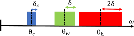
Figure 2: Scheme of the spectral windows assumed in Fig. 3 for the simulation of the cooling current and the cooling COP. We vary $\beta_{h}$ and $\delta$ fixing $\beta_{c}=1$, $\beta_{w}=0.1$, $\theta_{c}=2$, $\theta_{h}=6$, $\theta_{w}=4$, $\omega_{0}=0$, $\epsilon_{\nu}=1$ We use the form (39) with $p=1$, $\delta_{c}=0.2$, $\delta_{w}=\delta$ and $\delta_{h}=2\delta$. The rectangular boxes represent the windows over which the functions $M_{\nu}(\omega)$ are defined—in the domain of positive frequencies. Corresponding functions appear in the negative range, decorated by a detailed balance factor $e^{\beta_{\nu}\omega}$.

In Fig. 3, we display the cooling current and the cooling COP for the model of Fig. 2. The current $J_{c}/C_{3}$ is dimensionless, with $C_{3}\propto\gamma^{2}$, $\gamma$ as the system-bath interaction energy, see text below Eq. (10). To receive the current in physical units of e.g. J/sec, one should further divide it by $\hbar$. We find that the system can act as a refrigerator within a certain domain: According to the ideal case, Eq. (15), cooling takes place when $\beta_{h}\geq\frac{\theta_{c}}{\theta_{h}}(\beta_{c}-\beta_{w})+\beta_{w}$. In our parameters, this reduces to $\beta_{h}\geq 0.9/3+0.1=0.4$. This estimate qualitatively agrees with simulations at small $\delta$.

The width parameter is important as well, and we find that refrigeration takes place as long as $\delta\lesssim 1.6$. Note that when $\delta\geq 1.8$, the functions $M_{c}(\omega)$ and $M_{w}(\omega)$ overlap leading to energy leakage directly from the work bath to the cold environment. Nevertheless, it is interesting to note that the hot and work reservoirs already touch when $\delta\geq 2/3$, yet their overlap does not prohibit the cooling process. Overall, temperature, $\theta_{\nu}$, and the width parameters $\delta_{\nu}$ intermingle in the expression for cooling. As a result, the cooling window depends on $\delta$ in a non-trivial manner. As an additional comment, in Fig. 3, we consistently receive $\eta<\theta_{c}/\theta_{w}=0.5$. However, when using a narrower window for the cold bath, e.g., $\delta_{c}\sim 0.1$, we find that in fact the cooling COP can exceed $1/2$, yet obviously it still lies below the Carnot bound.

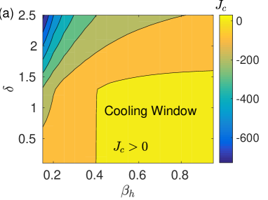
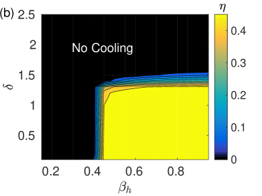
Figure 3: (a) Cooling window and (b) corresponding cooling COP for the configuration described in Fig. 2.

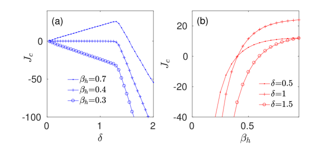
Figure 4: Slices of cooling current from Fig. 3. (a) $J_{c}$ as a function of $\delta$ for three values of $\beta_{h}$. (b) $J_{c}$ as a function of $\beta_{h}$ for three values of $\delta$. Other parameters are the same as indicated in Fig. 2.

In Fig. 4, we display slices of the cooling current as a function of the width $\delta$ and temperature $\beta_{h}$, taken from the contour plot, Fig. 3. For small value of $\delta$ the cooling current grows linearly. However, at a certain point ($\delta=1.3$), when the cold and work reservoirs almost touch, the cooling current begins to drop with $\delta$, eventually missing the cooling operation altogether. The behavior of the cooling current with $\beta_{h}$ is monotonic.

The role of a nonzero gap $\omega_{0}\neq 0$ on the operation of the qubit-QAR is presented in Fig. 5, using again parameters as in Fig. 2. In panel (a), we set $\delta=1$. We find that within the cooling window, the performance of the QAR is intact for small $\omega_{0}$, but it deteriorates and eventually disappears once $\omega_{0}$ is comparable to differences of the central frequencies, $\theta_{\nu}$. Outside the cooling window, for large $\delta$, in panel (b) we reveal a non-trivial non-monotonic behavior of $J_{c}$ with $\omega_{0}$, with a large value of $\omega_{0}$ manifesting a cooling function that is missing in the degenerate case. Overall, as long as $\omega_{0}\ll\delta$, it plays an insignificant role in the refrigeration behavior. Beyond that, it can introduce cooling, enhance or reduce performance, depending on the particular choice of parameters.

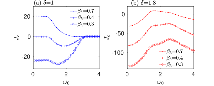
Figure 5: Cooling current as a function of the qubit energy gap $\omega_{0}$ for the parameters of Fig. 2-3 for $\beta_{h}=0.3,0.4,0.7$, bottom to top, and (a) $\delta=1$ , (b) $\delta=1.8$.

V Physical model

Before concluding, we discuss physical models corresponding to the model Hamiltonian (4) and the functions $M_{\nu}(\omega)$. We assume that the baths include collections of harmonic oscillators, $\hat{H}_{B,\nu}=\sum_{j}\omega_{j,\nu}\hat{b}_{j,\nu}^{\dagger}\hat{b}_{j,\nu}$, and that bath operators, which are coupled to the system, are of the form

$$\hat{B}_{\nu}=\sum_{j}\frac{\lambda_{j,\nu}}{\omega_{j,\nu}}\left(\hat{b}_{j,\nu}^{\dagger}+\hat{b}_{j,\nu}\right).$$ (40)

The two-time correlation functions are thus given by

$$M_{\nu}(t)=\langle\hat{B}_{j,\nu}(t)\hat{B}_{j,\nu}(0)\rangle=\sum_{j}\frac{\lambda_{j,\nu}^{2}}{\omega_{j,\nu}^{2}}\left[n_{\nu}(\omega_{j,\nu})e^{i\omega_{j,\nu}t}+(n_{\nu}(\omega_{j,\nu})+1)e^{-i\omega_{j,\nu}t}\right],$$ (41)

with $n_{\nu}(\omega)=[e^{\beta_{\nu}\omega}-1]^{-1}$ as the Bose-Einstein distribution function. In the frequency domain,

$$M_{\nu}(\omega)=2\pi\sum_{j}\frac{\lambda_{j,\nu}^{2}}{\omega_{j,\nu}^{2}}\left[n_{\nu}(\omega_{j,\nu})\delta(\omega+\omega_{j,\nu})+(n_{\nu}(\omega_{j,\nu})+1)\delta(\omega-\omega_{j,\nu})\right].$$ (42)

We now define the spectral density function, which is related to the density of states of the bath,

$$g_{\nu}(\omega)=2\pi\sum_{j}\frac{\lambda_{j,\nu}^{2}}{\omega_{j,\nu}^{2}}\delta(\omega-\omega_{j,\nu}),$$ (43)

and find that,

$$M_{\nu}(\omega)=\left[n_{\nu}(\omega)+1\right]g_{\nu}(\omega)$$ (44)

with $g_{\nu}(\omega)$ analytically continued to the complete real axis as an odd function. According to Eq. (44), the function $M_{\nu}(\omega)$ is linearly related to the spectral density function $g_{\nu}(\omega)$ of the respective bath. Thus, if we can engineer the density of states of the bath, or filter its frequencies, we can realize a structured model of the form (16).

Let us now also comment on the relation of the Hamiltonian (4) to the nonequilibrium (multi-bath) spin-boson Hamiltonian. We begin with the additive model,

$$\hat{H}=\frac{\omega_{0}}{2}\hat{\sigma}_{z}+\frac{\Delta}{2}\hat{\sigma}_{x}+\sum_{\nu,j}\omega_{j,\nu}\hat{b}_{j,\nu}^{\dagger}\hat{b}_{j,\nu}+\hat{\sigma}_{z}\sum_{\nu,j}\lambda_{j,\nu}\left(\hat{b}_{j,\nu}^{\dagger}+\hat{b}_{j,\nu}\right),$$ (45)

and transform it to the displaced bath-oscillators basis using the small polaron transformation Mahan , $\hat{H}_{p}=\hat{U}^{\dagger}\hat{H}\hat{U}$, $\hat{U}=e^{i\hat{\sigma}_{z}\hat{\Omega}/2}$,

$$\hat{H}_{p}=\frac{\omega_{0}}{2}\hat{\sigma}_{z}+\frac{\Delta}{2}\left(\hat{\sigma}_{+}e^{i\hat{\Omega}}+\hat{\sigma}_{-}e^{-i\hat{\Omega}}\right)+\sum_{\nu,j}\omega_{j,\nu}\hat{b}_{j,\nu}^{\dagger}\hat{b}_{j,\nu}.$$ (46)

Here, $\hat{\sigma}_{\pm}=\frac{1}{2}(\hat{\sigma}_{x}\pm i\hat{\sigma}_{y})$ are the auxiliary Pauli matrices, $\hat{\Omega}=\sum_{\nu}\hat{\Omega}_{\nu}$, $\hat{\Omega}_{\nu}=2i\sum_{j}\frac{\lambda_{j,\nu}}{\omega_{j}}(\hat{b}_{j,\nu}^{\dagger}-\hat{b}_{j,\nu})$. It can be shown that under the so-called noninteracting blip approximation Weiss ; Legget ; Dekker , the population dynamics follows Eq. (5) with the time correlation function

$$M_{\nu}(t)=\langle e^{i\Omega(t)}e^{-i\Omega(0)}\rangle=e^{-Q_{\nu}(t)}.$$ (47)

The average is performed with respect to the initial, product thermal state of the baths. The function $Q(t)=\sum_{\nu}{Q_{\nu}(t)}$ is complex, with real and imaginary components, $Q_{\nu}(t)=Q^{\prime}_{\nu}(t)+iQ^{\prime\prime}_{\nu}(t)$,

$$Q^{\prime\prime}_{\nu}(t) = 2\int_{0}^{\infty}\frac{g_{\nu}(\omega)}{\pi}\sin(\omega t)d\omega,$$

$$Q^{\prime}_{\nu}(t) = 2\int_{0}^{\infty}\frac{g_{\nu}(\omega)}{\pi}[1-\cos(\omega t)][1+2n_{\nu}(\omega)]d\omega.$$ (48)

The multi-bath spin-boson example clearly demonstrates that non-additivity of the interaction Hamiltonian embodies strong coupling effects. Using Eq. (46) as a starting point, a second order time-evolution scheme with respect to $\Delta$ provides an equation of motion for the population dynamics in the form (5), which is beyond second order in the system-bath interaction energy $\lambda$ segal-nicolin . Nevertheless, to realize a QAR we need to design the function $M_{\nu}(t)$, which is the central object in the expressions for the population and energy current. For the spin-boson model, this function, [see Eqs. (47)-(48)], depends in a non-linear manner on the reservoirs’ density of states, thus it is not immediately clear how to physically-rationally engineer it to receive the form (16).

VI Summary and Outlook

What is the smallest possible fridge? Using a quantum master equation in Lindblad form with additive dissipators, it was argued in Ref. PopescuPRL that a three-level system (qutrit) is the smallest refrigerator, if each transition is thermalized independently. Here, we demonstrate that in fact a qubit could serve as smallest refrigerator—if the three thermal reservoirs $c$, $h$ and $w$ couple in a non-additive manner to the qubit, to transfer energy in a cooperative manner. Our formalism is consistent with classical thermodynamics, as it complies with the heat exchange fluctuation theorem.

In the ideal limit we receive refrigeration if (i) the reservoirs are engineered, and are allowed to exchange energy within a highly restricted spectral window, (ii) a resonant condition $\theta_{c}+\theta_{w}=\theta_{h}$ is satisfied for the characteristic frequencies of the three reservoirs. In this special situation, we derived closed expressions for the cooling window, the efficiency of the refrigerator (characterized by its COP), the maximal efficiency (bounded by the Carnot limit) and the maximum-power efficiency. We found that a qubit-QAR with a non-additive dissipation form can embody function that is prohibited under the weak system-bath coupling assumption. We had further studied, analytically and numerically, the operation of the system beyond the ideal limit and found that it can operate as a QAR for a fair range of parameters.

Throughout this study, we had assumed a resonance condition (12) for the characteristic frequencies of the three reservoirs, so as to optimize performance. Nevertheless, it is imperative to realize that one could construct a qubit-QAR without structuring the work reservoir. Going back to Eq. (11), we evaluate the cooling current when the cold and hot FBCF take the form of a Dirac delta function as in Eq. (13), with $\theta_{h}>\theta_{c}>0$, but the work reservoir’s FBCF is simply a constant, $M_{w}(\omega)=\epsilon_{w}$ for $\omega\geq 0$. We then obtain a modified cooling window (compare to Eq. (14)),

$$\theta_{c}\left(e^{-\beta_{c}\theta_{c}}e^{-\beta_{w}(\theta_{h}-\theta_{c})}-e^{-\beta_{h}\theta_{h}}\right)+\theta_{c}\left(e^{-\beta_{c}\theta_{c}}e^{-\beta_{h}\theta_{h}}-e^{-\beta_{w}(\theta_{c}+\theta_{h})}\right)\geq 0.$$ (49)

The new, last two terms correspond to the extraction of energy from the cold bath, assisted by the hot bath, to be dumped into the work reservoir, and the reversed process. We can reorganize the cooling condition as

$$e^{-\beta_{c}\theta_{c}}e^{-\beta_{w}(\theta_{h}-\theta_{c})}-e^{-\beta_{h}\theta_{h}}(1+A)\geq 0,$$ (50)

where $A\equiv e^{-\beta_{w}(\theta_{c}+\theta_{h})}e^{\beta_{h}\theta_{h}}-e^{-\beta_{c}\theta_{c}}$. After some manipulations, we arrive at

$$\frac{\theta_{c}}{\theta_{h}}\leq\frac{\beta_{h}-\beta_{w}}{\beta_{c}-\beta_{w}}-\frac{1}{\theta_{h}(\beta_{c}-\beta_{w})}\ln(1+A).$$ (51)

Since $A>0$, it is clear that the cooling window is reduced here relative to the case with a structured work bath, (15). This new situation is significant: We do not place here stringent conditions on the work reservoir, which could in fact be featureless and still support cooling. Furthermore, this scenario, where the work reservoir is allowed to provide or absorb both low and high frequencies, is obviously un-accounted for in the traditional three-level weak-coupling setting where each bath excites a particular transition in a resonant manner (see Fig. 1)(a). A strongly-coupled qubit-QAR thus offers new regimes of operation, missing in multi-level, weakly coupled designs.

We examined an additive dissipation model and proved that it cannot support a QAR performance based on a qubit. In contrast, a non-additive model, with the three reservoirs acting in a concerted manner, can achieve refrigeration. It is of an interest to examine an in-between model, which could be more practical. For example, the cold and work reservoirs could couple strongly to build up a non-additive dissipator, but the hot bath would weakly-separately couple to the system, bringing in an additional, local dissipation term. This scenario could be treated using the reaction coordinate method Gernot or the polaron-transformed master equation Ren1 ; Ren2 ; Schallerpol1 ; Schallerpol2 , which can smoothly interpolate between additive and non-additive dissipation problems.

The description of quantum systems that are strongly coupled to multiple thermal reservoirs poses a significant theoretical challenge. Markovian master equations of Lindblad form with additive (local) dissipators provide a consistent thermodynamical description of observables kos13 . However, it is not yet established how to formulate quantum thermodynamics beyond the weak coupling limit. Our work here exemplifies a strong coupling framework which is thermodynamically consistent. It is of interest to compare our approach and predictions to other recent studies on strongly-coupled energy conversion devices DavidS ; Kosloff ; Cao ; Gernot ; Jarzynski ; esposito17 ; Nazir , and further develop numerically exact techniques that could target such problems. Understanding the role of both strong coupling and non-Markovianity of the reservoirs on the operation of driven and autonomous thermal machines remains a challenge for future work.

Appendix A: Cooling condition for a non-degenerate Qubit-QAR

We investigate here the cooling performance of a qubit of a finite energy gap $\omega_{0}$. For simplicity, we assume the following functions ($\omega>0$). The negative-frequency branch is decorated by detailed-balance (thermal) factors,

$$M_{c}(\omega) = \epsilon_{c}\delta(\omega-\theta_{c}),$$

$$M_{h}(\omega) = \epsilon_{h}\left[\delta(\omega-\theta_{h}-\omega_{0})+\delta(\omega-\theta_{h}+\omega_{0})\right],$$

$$M_{w}(\omega) = \epsilon_{w}\delta(\omega-\theta_{w}).$$ (A1)

Here, $\epsilon_{c,h,w}$ are dimensionless parameters. Since these parameters do not influence the cooling window and the cooling efficiency, we ignore them below. We maintain the resonant condition, $\theta_{c}+\theta_{w}=\theta_{h}$. We further assume that $\omega_{0}$ is much smaller than $\theta_{\nu},\nu=c,h,w$.

One should note that the steady-state populations of the qubit are no-longer equal. We will begin by evaluating them from Eq. (5). The three-bath convoluted decay rate is

$$M(\omega_{0})=\int_{-\infty}^{\infty}d\omega_{1}M_{c}(\omega_{1})\int_{-\infty}^{\infty}d\omega_{2}M_{h}(\omega_{2})M_{w}(\omega_{0}-\omega_{1}-\omega_{2}).$$ (A2)

We break the integral into four contributions. For $\omega_{1}\geq 0$, $\omega_{2}\geq 0$,

$$M(\omega_{0}) = \int_{0}^{\infty}d\omega_{1}M_{c}(\omega_{1})\int_{0}^{\infty}d\omega_{2}M_{h}(\omega_{2})M_{w}(\omega_{0}-\omega_{1}-\omega_{2})$$ (A3)

$$= 0,$$

since we assume that $\omega_{0}$ is sufficiently small, such that $\theta_{c}+\theta_{h}-2\omega_{0}>\theta_{w}$. Similarly, when $\omega_{1}\leq 0$, $\omega_{2}\leq 0$,

$$M(\omega_{0}) = \int_{-\infty}^{0}d\omega_{1}M_{c}(\omega_{1})\int_{-\infty}^{0}d\omega_{2}M_{h}(\omega_{2})M_{w}(\omega_{0}-\omega_{1}-\omega_{2})$$ (A4)

$$= 0.$$

We receive a finite contribution when $\omega_{1}\geq 0$ and $\omega_{2}\leq 0$,

$$M(\omega_{0}) = \int_{0}^{\infty}d\omega_{1}M_{c}(\omega_{1})\int_{-\infty}^{0}d\omega_{2}M_{h}(\omega_{2})M_{w}(\omega_{0}-\omega_{1}-\omega_{2})$$ (A5)

$$= \int_{0}^{\infty}d\omega_{1}M_{c}(\omega_{1})\int_{0}^{\infty}d\omega_{2}M_{h}(\omega_{2})e^{-\beta_{h}\omega_{2}}M_{w}(\omega_{0}-\omega_{1}+\omega_{2})$$

$$= e^{-\beta_{h}(\theta_{h}-\omega_{0})},$$

as well as for $\omega_{1}\leq 0$, and $\omega_{2}>0$,

$$M(\omega_{0}) = \int_{-\infty}^{0}d\omega_{1}M_{c}(\omega_{1})\int_{0}^{\infty}d\omega_{2}M_{h}(\omega_{2})M_{w}(\omega_{0}-\omega_{1}-\omega_{2})$$ (A6)

$$= \int_{0}^{\infty}d\omega_{1}M_{c}(\omega_{1})e^{-\beta_{c}\omega_{1}}\int_{0}^{\infty}d\omega_{2}M_{h}(\omega_{2})M_{w}(\omega_{0}+\omega_{1}-\omega_{2})$$

$$= \int_{0}^{\infty}d\omega_{1}M_{c}(\omega_{1})e^{-\beta_{c}\omega_{1}}\int_{0}^{\infty}d\omega_{2}M_{h}(\omega_{2})M_{w}(\omega_{2}-\omega_{1}-\omega_{0})e^{-\beta_{w}(\omega_{2}-\omega_{1}-\omega_{0})}$$

$$= e^{-\beta_{c}\theta_{c}}e^{-\beta_{w}\theta_{w}}.$$

Therefore, we find that $M(\omega_{0})=e^{-\beta_{h}(\theta_{h}-\omega_{0})}+e^{-\beta_{c}\theta_{c}}e^{-\beta_{w}\theta_{w}}$. Similarly, $M(-\omega_{0})=e^{-\beta_{h}(\theta_{h}+\omega_{0})}+e^{-\beta_{c}\theta_{c}}e^{-\beta_{w}\theta_{w}}$. In steady state, the populations follow $p_{g}=\frac{M(\omega_{0})}{M(\omega_{0})+M(-\omega_{0})}$ and $p_{e}=\frac{M(-\omega_{0})}{M(\omega_{0})+M(-\omega_{0})}$. Our results reduce to $p_{g,e}=1/2$ when $\omega_{0}=0$.

We now turn to the expression for the cooling current, Eq. (10). It is easy to calculate the integrals in this equation since there is only one extra $\omega_{1}$ term, which is trivial to account for under (A1). We evaluate the two integrals,

$$I_{1} \equiv -\int_{-\infty}^{\infty}\int_{-\infty}^{\infty}d\omega_{1}d\omega_{2}\omega_{1}M_{c}(\omega_{1})M_{h}(\omega_{2})M_{w}(\omega_{0}-\omega_{1}-\omega_{2})$$ (A7)

$$= \theta_{c}(e^{-\beta_{c}\theta_{c}}e^{-\beta_{w}\theta_{w}}-e^{-\beta_{h}\theta_{h}}e^{\beta_{h}\omega_{0}}),$$

and

$$I_{2} \equiv \int_{-\infty}^{\infty}\int_{-\infty}^{\infty}d\omega_{1}d\omega_{2}\omega_{1}M_{c}(-\omega_{1})M_{h}(-\omega_{2})M_{w}(-\omega_{0}+\omega_{1}+\omega_{2})$$ (A8)

$$= \theta_{c}(e^{-\beta_{c}\theta_{c}}e^{-\beta_{w}\theta_{w}}-e^{-\beta_{h}\theta_{h}}e^{-\beta_{h}\omega_{0}}).$$

In total, the cooling current is

$$J_{c} = -p_{e}\int_{-\infty}^{\infty}\int_{-\infty}^{\infty}d\omega_{1}d\omega_{2}\omega_{1}M_{c}(\omega_{1})M_{h}(\omega_{2})M_{w}(\omega_{0}-\omega_{1}-\omega_{2})$$ (A9)

$$+ p_{g}\int_{-\infty}^{\infty}\int_{-\infty}^{\infty}d\omega_{1}d\omega_{2}\omega_{1}M_{c}(-\omega_{1})M_{h}(-\omega_{2})M_{w}(-\omega_{0}+\omega_{1}+\omega_{2})$$

$$= \frac{\theta_{c}}{M(\omega_{0})+M(-\omega_{0})}\left(e^{-\beta_{c}\theta_{c}}e^{-\beta_{w}\theta_{w}}+e^{-\beta_{h}\theta_{h}}e^{-\beta_{h}\omega_{0}}\right)\left(e^{-\beta_{c}\theta_{c}}e^{-\beta_{w}\theta_{w}}-e^{-\beta_{h}\theta_{h}}e^{\beta_{h}\omega_{0}}\right)$$

$$+ \frac{\theta_{c}}{M(\omega_{0})+M(-\omega_{0})}\left(e^{-\beta_{c}\theta_{c}}e^{-\beta_{w}\theta_{w}}+e^{-\beta_{h}\theta_{h}}e^{\beta_{h}\omega_{0}}\right)\left(e^{-\beta_{c}\theta_{c}}e^{-\beta_{w}\theta_{w}}-e^{-\beta_{h}\theta_{h}}e^{-\beta_{h}\omega_{0}}\right)$$

$$= \frac{2\theta_{c}}{M(\omega_{0})+M(-\omega_{0})}\left(e^{-2\beta_{c}\theta_{c}}e^{-2\beta_{w}\theta_{w}}-e^{-2\beta_{h}\theta_{h}}\right).$$

The cooling window, $J_{c}\geq 0$, precisely follows Eq. (14)—obtained for the case $\omega_{0}=0$.

Appendix B: Un-attainability of cooling for continuous-Gaussian spectral functions.

As we showed in the main text, functions $M_{\nu}(\omega)$ of restricted range support the cooling function in a qubit-QAR when the interaction of the qubit with the separate baths is made non-additive. We now examine an example with functions that are non-zero in the full range, without any filtering, and show that the system cannot act as a QAR.

We assume a Gaussian form for the FBCF, $M_{\nu}(\omega)=\sqrt{\frac{\pi}{E_{r}^{\nu}T_{\nu}}}\exp\left(-\frac{(\omega-E_{r}^{\nu})^{2}}{4E_{r}^{\nu}T_{\nu}}\right)$, which describes bath-induced rates in the spin-boson model at high temperature. Specifically, performing a short time expansion of Eq. (48), we get $Q^{{}^{\prime\prime}}_{\nu}(t)=\frac{2}{\pi}t\int d\omega g_{\nu}(\omega)\omega$ and $Q^{{}^{\prime}}_{\nu}(t)=\frac{2T_{\nu}}{\pi}t^{2}\int d\omega g_{\nu}(\omega)\omega$. Defining $E_{r}^{\nu}\equiv\frac{2}{\pi}\int d\omega g_{\nu}(\omega)\omega$, we arrive at $Q^{{}^{\prime\prime}}_{\nu}(t)=E_{r}^{\nu}t$ and $Q^{{}^{\prime}}_{\nu}(t)=E_{r}^{\nu}T_{\nu}t^{2}$. The energy scale $E_{r}^{\nu}$ is referred to as the “reorganization energy”, and it represents the strength of the system-bath interaction. The current from the cold bath is given by Eq. (11), which solves to

$$J_{c} = -\frac{1}{2}\int_{-\infty}^{\infty}\int_{-\infty}^{\infty}d\omega_{1}d\omega_{2}\omega_{1}M_{c}(\omega_{1})M_{h}(\omega_{2})M_{w}(-\omega_{1}-\omega_{2})+\frac{1}{2}\int_{-\infty}^{\infty}d\omega_{1}d\omega_{2}\omega_{1}M_{c}(-\omega_{1})M_{h}(-\omega_{2})M_{w}(\omega_{1}+\omega_{2})$$ (B1)

$$= -\frac{1}{2}\int_{-\infty}^{\infty}\int_{-\infty}^{\infty}d\omega_{1}\omega_{1}M_{c}(\omega_{1})\int_{-\infty}^{\infty}d\omega_{2}M_{h}(\omega_{2})M_{w}(\omega_{1}+\omega_{2})\left[e^{-\beta_{w}(\omega_{1}+\omega_{2})}-e^{-\beta_{c}\omega_{1}}e^{-\beta_{h}\omega_{2}}\right]$$

$$= 4E_{r}^{c}{\pi}^{\frac{5}{2}}\frac{E_{r}^{h}(T_{c}-T_{h})+E_{r}^{w}(T_{c}-T_{w})}{(E_{r}^{c}T_{c}+E_{r}^{h}T_{h}+E_{r}^{w}T_{w})^{\frac{3}{2}}}\exp\left(-\frac{(E_{r}^{c}+E_{r}^{h}+E_{r}^{w})^{2}}{4(E_{r}^{c}T_{c}+E_{r}^{h}T_{h}+E_{r}^{w}T_{w})}\right).$$

Since this expression is always negative, the system cannot act as a QAR. We can rationalize this result as follows. Let us define an effective temperature

$$T^{*}\equiv\frac{E_{r}^{c}T_{c}+E_{r}^{h}T_{h}+E_{r}^{w}T_{w}}{E_{r}^{c}+E_{r}^{h}+E_{r}^{w}},$$ (B2)

and the total interaction-reorganization energy, $E_{r}\equiv\sum_{\nu}E_{r}^{\nu}$. We can then recast $J_{c}$ of Eq. (B1) as follows,

$$J_{c}\propto\frac{1}{\sqrt{T^{*}E_{r}}}\frac{\left(T_{c}-T^{*}\right)}{T^{*}}e^{-E_{r}/4T^{*}}.$$ (B3)

Since $T^{*}>T_{c}$, cooling is prohibited. We now understand that, since the reservoirs can absorb and emit all frequency components, the system (qubit) can in fact be characterized by an effective interaction energy and an effective temperature, the latter is always greater than $T_{c}$ due to the cumulative effect of the other baths. As a result, it is impossible to extract energy from the cold bath. This argument suggests that finite-range hard-cutoff functions should be used to design a QAR, as we explain in the main body of the paper.

References

- (1) J. M. Gordon, K. C. Ng, Cool Thermodynamics Cambridge, UK: Cambridge Int. Sci. 2000.
- (2) S. Vinjanampathy and J. Anders, Contemporary Physics 57, 1 Taylor and Francis (2016).
- (3) R. Kosloff, Entropy 15, 2100 (2013).
- (4) R. Kosloff and A. Levy, Ann. Rev. Phys. Chem. 65, 365 (2014).
- (5) M. O. Scully, M. S. Zubairy, G. S. Agarwal, and H. Walther, Science 299, 862 (2003).
- (6) M. O. Scully, K. R. Chapin, K. E. Dorfman, M. B. Kim, and A. Svidzinsky, Proc. Natl. Acad. Sci. (U.S.A.) 108, 15097 (2011).
- (7) K. E. Dorfman, D. V. Voronine, S. Mukamel, and M. O. Scully, Proc. Natl. Acad. Sci. (U.S.A.) 110, 2746 (2013).
- (8) M. T. Mitchison, M. P. Woods, J. Prior, and M. Huber, New J. Phys. 17, 115013 (2015).
- (9) P. Kammerlander and J. Anders, Sci. Rep. 6, 22174 (2016).
- (10) J. Rosnagel, O. Anah, F. Schmidt-Kaler, K. Singer, and E. Lutz, Phys. Rev. Lett. 112, 030602 (2014).
- (11) R. Alicki and D. Gelbwaser-Klimovsky, New J. Phys. 17, 115012 (2015).
- (12) B. K. Agarwalla, J.-H. Jiang, and D. Segal, arXiv:1706.06206
- (13) G. Manzano, F. Galve, R. Zambrini, and J. M. R. Parrondo, Phys. Rev. E 93, 052120 (2016).
- (14) R. Alicki and M. Fannes, Phys. Rev. E 87, 042123 (2013).
- (15) M. Perarnau-Llobet, K. V. Hovhannisyan, M. Huber, P. Skrzypczyk, N. Brunner, and A. Acin, Phys. Rev. X 5, 041011 (2015).
- (16) N. Erez, G. Gordon, M. Nest, and G. Kurizki, Nature 452, 724 (2008).
- (17) D. Gelbwaser-Klimovsky, N. Erez, and R. Alicki, Phys. Rev. A 88, 022112 (2013).
- (18) K. Jacobs, Phys. Rev. A 80, 012322 (2009).
- (19) P. Strasberg, G. Schaller, T. Brandes, and M. Esposito, Phys. Rev. E 88, 062107 (2013).
- (20) D. Gelbwaser-Klimovsky and A. Aspuru-Guzik, J. Phys. Chem. Lett. 6, 3477 (2015).
- (21) G. Katz and R. Kosloff, Entropy 18, 186 (2016).
- (22) D. Xu, C. Wang, Y. Zhao, and J. Cao, New J. Phys. 18, 023003 (2016).
- (23) P. Strasberg, G. Schaller, N. Lambert, and T. Brandes, New J. Phys. 18, 073007 (2016).
- (24) R. Gallego, A. Riera, and J. Eisert, New J. Phys. 16, 125009 (2014).
- (25) C. Jarzynski, Phys. Rev. X 7, 011008 (2017).
- (26) P. Strasberg and M. Esposito, Phys. Rev. E 95, 062101 (2017).
- (27) D. Newman, F. Mintert, and A. Nazir, Phys. Rev. E 95, 032139 (2017).
- (28) G. Giusteri, F. Recrosi, G. Schaller, and G. L. Celardo, Phys. Rev. E 96, 012113 (2017).
- (29) L. A. Correa, J. P. Palao, C. Adesso, and D. Alonso, Phys. Rev. E 042131 (2013).
- (30) L. A. Correa, J. P. Palao, D. Alonso, and G. Adesso, Sci. Rep. 4, 3949 (2014).
- (31) L. A. Correa, Phys. Rev. E 89, 042128 (2014).
- (32) H.-P. Breuer and F. Petruccione, The Theory of Open Quantum Systems, Oxford University Press, New York 2002.
- (33) D. Segal and A. Nitzan, Phys. Rev. Lett. 94, 034301 (2005).
- (34) D. Segal, Phys. Rev. B, 73, 205415 (2006).
- (35) G.-L. Ingold and Yu. V. Nazarov, Charge Tunneling Rates in Ultrasmall Junctions, in Single Charge Tunneling, NATO ASI Series B 294, Plenum Press (1992).
- (36) L. Nicolin and D. Segal, J. Chem. Phys. 135, 164106 (2011).
- (37) N. Boudjada and D. Segal, J. Phys. Chem. A 118, 11323 (2014).
- (38) E. Geva and R. Kosloff, J. Chem. Phys. 96, 3054 (1992).
- (39) T. Feldman, E. Geva, R. Kosloff, and P. Salomon, Am. J. Phys. 64, 485 (1996).
- (40) T. Feldmann and R. Kosloff, Phys. Rev. E 61, 4774 (2000).
- (41) K. Szczygielski, D. Gelbwaser-Klimovsky, and R. Alicki, Phys. Rev. E 87, 012120 (2013).
- (42) D. Segal and A. Nitzan, Phys. Rev. E. 73, 026109 (2006).
- (43) D. Segal, Phys. Rev. Lett. 101, 260601 (2008).
- (44) D. Segal, J. Chem. Phys. 130, 134510 (2009).
- (45) D. Gelbwaser-Klimovsky, R. Alicki, and G. Kurizki, Phys. Rev. E 87 012140 (2013).
- (46) A. Levy and R. Kosloff, Phys. Rev. Lett. 108, 070604 (2012).
- (47) M. T. Mitchison, M. Huber, J. Prior, M. P. Woods, and M. B. Plenio, Quantum Science and Technology 1, 015001 (2016).
- (48) G. Maslennikov, S. Ding, R. Hablutzel, J. Gan, A. Roulet, S. Nimmrichter, J. Dai, V. Scarani, and D. Matsukevich, arXiv:1702.08672
- (49) H. M. Friedman, B. K. Agarwalla, and D. Segal, In preparation.
- (50) C. Wang, J. Ren, and J. Cao, Sci. Rep. 5, 11787 (2015).
- (51) C. Wang, J. Ren, and J. Cao, Phys. Rev. A 95, 023610 (2017).
- (52) D. Segal, Phys. Rev. E 77, 021103 (2008).
- (53) F. L. Curzon and B. Ahlborn, American Journal of Physics 43, 22 (1975)
- (54) C. Van den Broeck, Phys. Rev. Lett. 95, 190602, (2005).
- (55) T. Schmiedl and U. Seifert, Europhysics Letters 81 (2), 20003 (2007).
- (56) M. Esposito, K. Lindenberg, and C. Van den Broeck, Phys. Rev. Lett. 102, 130602 (2009).
- (57) M. Esposito, R. Kawai, K. Lindenberg, and C. Van den Broeck, Phys. Rev. Lett. 105, 150603 (2010).
- (58) Y. Zhou and D. Segal, Phys. Rev. E 82, 011120 (2010).
- (59) G. Benenti, G. Casati, K. Saito, and R. S. Whitney, Phys. Rep. 694, 1 (2017).
- (60) G. D. Mahan, Many-particle physics (Plenum press, New York, 2000).
- (61) U. Weiss, Quantum Dissipative Systems (World Scientific, Singapore, 1993).
- (62) A. J. Legget et al., Rev. Mod. Phys. 59, 1 (1987).
- (63) H. Dekker, Phys. Rev. A 35, 1436 (1987).
- (64) N. Linden, S. Popescu, and P. Skrzypczyk, Phys. Rev. Lett. 105, 130401 (2010).
- (65) G. Schaller, T. Krause, T. Brandes, and M. Esposito, New J. Phys. 15, 033032 (2013).
- (66) T. Krause, T. Brandes, M. Esposito, and G. Schaller, J. Chem. Phys. 142, 134106 (2015).