Large-scale structure perturbation theory without losing stream crossing

Abstract

We suggest an approach to perturbative calculations of large-scale clustering in the Universe that includes from the start the stream crossing (multiple velocities for mass elements at a single position) that is lost in traditional calculations. Starting from a functional integral over displacement, the perturbative series expansion is in deviations from (truncated) Zel’dovich evolution, with terms that can be computed exactly even for stream-crossed displacements. We evaluate the one-loop formulas for displacement and density power spectra numerically in 1D, finding dramatic improvement in agreement with N-body simulations compared to the Zel’dovich power spectrum (which is exact in 1D up to stream crossing). Beyond 1D, our approach could represent an improvement over previous expansions even aside from the inclusion of stream crossing, but we have not investigated this numerically. In the process we show how to achieve effective-theory-like regulation of small-scale fluctuations without free parameters.

I Introduction

Perturbation theory for large-scale gravitational evolution and clustering in the Universe Bernardeau et al. (2002) should be increasingly valuable as large-scale structure (LSS) surveys become increasingly large and precise Font-Ribera et al. (2014); DESI Collaboration et al. (2016). From the beginning Zel’Dovich (1970), this kind of perturbation theory has had a nagging deficiency that there was no first-principles way to include “stream crossing” (often alternatively called “shell crossing”), i.e., multiple different velocities for mass at a single point in space. This is a purely technical problem—it is easy to write down the exact evolution equations for mass elements under effectively Newtonian gravity, and easy to see that stream crossing will happen, but we simply have not had any clean mathematical method to include this phenomenon and still produce perturbative analytic results for clustering statistics. In contrast, a wonderful thing about N-body simulations Davis et al. (1985); Feng et al. (2016) is they trivially include arbitrarily complex velocity structure at a point (pedantically, one can say that you never have more than one particle at a mathematical point, but we implicitly understand that the particles in simulations are really an approximation to some effectively continuous cloud). The key weakness appears in Lagrangian perturbation theory (LPT) Buchert and Ehlers (1993); Bouchet et al. (1995); Matsubara (2008a); Okamura et al. (2011); Rampf (2012); Vlah et al. (2015) because density is approximated by the Taylor expansion of the determinant of the local deformation tensor, which is only correct before stream crossing. Eulerian perturbation theory (EPT) is derived by truncating the evolution equations for moments of the velocity distribution function after the first moment, i.e., velocity dispersion is set to zero Peebles (1980); Goroff et al. (1986); McDonald (2011).

One unavoidable criticism of various efforts to improve perturbation theory by effectively summing to higher orders McDonald (2007, 2014); Taruya and Hiramatsu (2008) has been that we were summing a theory that was not exactly correct anyway, because of missing stream crossing Afshordi (2007). Pueblas and Scoccimarro (2009) found only small effects from stream crossing in numerical simulations; however, this does not mean that missing stream crossing necessarily has only a small effect on a given perturbation theory calculation. One of our findings here will be that stream crossing self-regulates, in the following sense: If you ignore it in force calculations, e.g., in the Zel’dovich approximation, the extrapolated amount of stream crossing and its effect on the density power spectrum is large (the exact Zel’dovich power spectrum does include stream crossing for a given displacement field). This makes the Zel’dovich power spectrum inaccurate, while including the effect of stream crossing on forces, feeding back to suppress itself, greatly improves the results. Of course, it is also simply desirable to compute small effects to match increasingly high precision observations.

There have been many efforts to include the effects of stream crossing in calculations. References Davis and Peebles (1977); McDonald (2011); Tassev (2011) included equations for moments of the velocity distribution, but this requires a truncation of the moment hierarchy and convergence was never demonstrated. The adhesion approximation of Gurbatov et al. (1989); Kofman and Shandarin (1988); Weinberg and Gunn (1990) aimed to make crossing streams stop and stick instead of crossing. Reference Pietroni et al. (2012) derived evolution equations for explicitly smoothed fields in which a coarse-grained velocity dispersion appears, with contributions to it beyond EPT to be computed by simulations. Baumann et al. (2012); Carrasco et al. (2012); Hertzberg (2014) introduced general “effective field theory” counter-terms with free coefficients that allow fitting for the stream crossing effect in simulations or data. Reference Aviles (2016) computed the velocity dispersion tensor implied by LPT. While many of these approaches have had significant success, we would like to find a more direct calculation.

Many elements of this paper have appeared before. The basic math we exploit to compute forces including stream crossing has been hiding in plain sight in the calculation of the exact Zel’dovich power spectrum (apparently computed first, at least in correlation function form, in Couchman and Bond (1988), which we could not find online—see Bernardeau et al. (2002)) which does include stream crossing but only for a given displacement field. Reference Valageas (2011) investigated the effect of stream crossing by comparing this Zel’dovich calculation to one where relative streams are stopped “by hand” when they would otherwise cross. Valageas and others have been using a similar functional integral formalism for many years Valageas (2001, 2002, 2004, 2007a); Matarrese and Pietroni (2007); Valageas (2007b, 2008); Skovbo (2012); Rigopoulos (2015); Führer and Rigopoulos (2016). The starting formalism of Bartelmann et al. (2016) is similar to ours except for discussing literal particles instead of a continuum limit, while Ali-Haïmoud (2015) is even more similar, although without the functional integral formalism. Reference Taruya and Colombi (2017) has a somewhat similar idea of integrating the force after stream crossing. It is generally understood that some form of damping of small-scale initial conditions is a good idea Crocce and Scoccimarro (2006a, b, 2008); Bernardeau and Valageas (2008); Bernardeau et al. (2008); Anselmi et al. (2011); Taruya et al. (2012); Sugiyama and Futamase (2012); Bernardeau et al. (2012). The decisive new feature in this paper is the specific straightforward perturbative expansion of the functional integral that we do, allowing concise calculation of statistical results. Stream crossing appears essentially effortlessly—in fact, if this was the first calculation a person ever saw, they probably would not realize stream crossing was a thing to worry about missing at all.

In the following sections we build up the calculation systematically, starting with nothing more than the basic equations for Newtonian gravitational evolution. Most of this is basically notation, that we think makes the calculations easier but is not fundamentally connected to the inclusion of stream crossing. A reader who would like to try to understand the key math trick that we use to avoid losing stream crossing without learning any of the formalism may want to read Appendix A first, where we attempt to give a pedagogical taste of what is going on in the main calculation.

II Evolution Equations

We start with the exact equations for the displacement field $\mathbf{\psi}(\mathbf{q})$ of mass elements labeled by their initial position (Lagrangian coordinate) $\mathbf{q}$, at physical position $\mathbf{x}(\mathbf{q})=\mathbf{q}+\mathbf{\psi}(\mathbf{q})$, and the velocity field $\mathbf{\upsilon}\equiv\mathbf{\psi}^{\prime}$, where we use prime to indicate a derivative with respect to $\eta\equiv\ln a$, which we will use as our primary time variable ($a$ is the expansion factor). We have, with dots for standard time derivative,

$$\ddot{\mathbf{\psi}}(\mathbf{q})+2H\dot{\mathbf{\psi}}(\mathbf{q})=\mathbf{F}\left[\mathbf{x}\left(\mathbf{q}\right)\right]=-\partial_{\mathbf{x}}V\left[\mathbf{x}\left(\mathbf{q}\right)\right]=-\partial_{\mathbf{x}}V\left[\mathbf{q}+\mathbf{\psi}\left(\mathbf{q}\right)\right]$$ (1)

with potential due to density fluctuations

$$V(\mathbf{x})=\frac{3}{2}\Omega_{m}H^{2}\partial_{\mathbf{x}}^{-2}\delta(\mathbf{x})$$ (2)

(see Bernardeau et al. (2002) for a comprehensive introduction to LSS perturbation theory). Density at position $\mathbf{x}$ is

$$1+\delta(\mathbf{x})=\int d^{d}\mathbf{q}~{}\delta^{D}\left[\mathbf{x}-\mathbf{q}-\mathbf{\psi}\left(\mathbf{q}\right)\right]=\int d^{d}\mathbf{q}\int\frac{d^{d}\mathbf{k}}{\left(2\pi\right)^{d}}e^{-i\mathbf{k}\cdot\left[\mathbf{x}-\mathbf{q}-\mathbf{\psi}\left(\mathbf{q}\right)\right]}~{},$$ (3)

or in (Eulerian) Fourier space

$$\delta(\mathbf{k})=\int d^{d}\mathbf{q}~{}e^{i\mathbf{k}\cdot\mathbf{q}}\left[e^{i\mathbf{k}\cdot\mathbf{\psi}\left(\mathbf{q}\right)}-1\right]~{}.$$ (4)

The density at particle $\mathbf{q}$, i.e., at position $\mathbf{x}(\mathbf{q})=\mathbf{q}+\mathbf{\psi}\left(\mathbf{q}\right)$, is

$$1+\delta\left[\mathbf{x}\left(\mathbf{q}\right)\right]=\int d^{d}\mathbf{q}^{\prime}\int\frac{d^{d}\mathbf{k}}{\left(2\pi\right)^{d}}e^{-i\mathbf{k}\cdot\left[\mathbf{q}+\mathbf{\psi}\left(\mathbf{q}\right)-\mathbf{q}^{\prime}-\mathbf{\psi}\left(\mathbf{q}^{\prime}\right)\right]}~{}.$$ (5)

So finally the force on mass element $\mathbf{q}$ at $\mathbf{x}(\mathbf{q})$ is

$$\mathbf{F}\left[\mathbf{x}\left(\mathbf{q}\right)\right]=-\frac{3}{2}\Omega_{m}H^{2}\int d^{d}\mathbf{q}^{\prime}\frac{d^{d}\mathbf{k}}{\left(2\pi\right)^{d}}\frac{i\mathbf{k}}{k^{2}}\left[e^{-i\mathbf{k}\cdot\left[\mathbf{q}+\mathbf{\psi}\left(\mathbf{q}\right)-\mathbf{q}^{\prime}-\mathbf{\psi}\left(\mathbf{q}^{\prime}\right)\right]}-e^{-i\mathbf{k}\cdot\left[\mathbf{q}+\mathbf{\psi}\left(\mathbf{q}\right)-\mathbf{q}^{\prime}\right]}\right]~{},$$ (6)

where we have included the second term, coming from the mean (background) part of the density, subtracted in the definition of $\delta\equiv\rho/\bar{\rho}-1$, because it definitely does produce a force—the force that decelerates the Hubble flow—which must be subtracted out of the first term here. To help clarify: $\mathbf{\psi}(\mathbf{q}^{\prime})$ here represents the displacements of the mass doing the forcing, while $\mathbf{\psi}(\mathbf{q})$ is the displacement of the mass being forced, which could just as well be a negligible test mass, which is why it makes sense for it to appear in the homogeneous part. If $\mathbf{\psi}(\mathbf{q}^{\prime})=0$ the forcing field is homogeneous so the peculiar acceleration is zero.

Note that when we write formulas with general dimensionality $d$ here, we are not really implying a Universe with fundamentally $d$ dimensions. We are following McQuinn and White (2016) in modeling a 3D background Universe with reduced dimensionality fluctuations, i.e., if $\mathbf{\psi}(\mathbf{q})$ does not depend on a component of $\mathbf{q}$, it is easy to see that we can integrate this component out of all these equations, leaving the reduced $d$ accounting for only directions that fluctuate. If it is not obvious that the qualification that the background Universe is still 3D matters, note that in a 1D background, with no cosmological constant, in the Newtonian limit, the force between particles is constant, i.e., does not diminish with expansion. This means that a truly 1D Universe will always turn around and collapse eventually, i.e., there is no concept of an Einstein-de Sitter (EdS) Universe with power law expansion.

Specializing to EdS for simplicity, and substituting in $\mathbf{\upsilon}$ to produce a 1st order equation, we can write Eq. (1) as

$$\mathbf{\upsilon}^{\prime}+\frac{1}{2}\mathbf{\upsilon}-\frac{3}{2}\psi=-\frac{3}{2}\partial_{\mathbf{x}}\partial_{\mathbf{x}}^{-2}\delta-\frac{3}{2}\psi$$ (7)

where note that we have subtracted $\frac{3}{2}\psi$ from both sides to make the left-hand side correspond to the linearized Zel’dovich evolution, while the right-hand side is the force beyond this. We can combine $\mathbf{\psi}$ and $\mathbf{\upsilon}$ into a single vector

$$\mathbf{\phi}\equiv\left(\begin{array}[]{c}\mathbf{\psi}\\ \mathbf{\upsilon}\end{array}\right)$$ (8)

and, understanding $\mathbf{\phi}=[\mathbf{\phi}]_{i}^{\alpha}(\eta,\mathbf{q})$ as a vector in $\infty\times\infty^{d}\times d\times 2$ dimensional space, labeled by time, $d$ spatial coordinates, their standard spatial vector direction, and $\mathbf{\psi}$ or $\mathbf{\upsilon}$, write the entire system compactly as

$$\mathbf{L}_{0}\mathbf{\phi}+\mathbf{\Delta}_{0}(\mathbf{\phi})=\mathbf{\epsilon}~{},$$ (9)

where $\mathbf{L}_{0}$ is a matrix acting in this $\infty\times\infty^{d}\times d\times 2$ dimensional space, with elements

$$[\mathbf{L}_{0}]_{i_{2}i_{1}}(\mathbf{q}_{2},\eta_{2},\mathbf{q}_{1},\eta_{1})=\left(\begin{array}[]{cc}\frac{\partial}{\partial\eta_{2}}&-1\\ -\frac{3}{2}&\frac{\partial}{\partial\eta_{2}}+\frac{1}{2}\\ \end{array}\right)\delta^{D}(\eta_{2}-\eta_{1})\delta^{K}_{i_{2}i_{1}}\delta^{D}(\mathbf{q}_{2}-\mathbf{q}_{1})$$ (10)

[where the explicit matrix is over $(\psi,\upsilon)$ and Kronecker-$\delta$ over spatial directions—note that in Fourier space with coordinate $\mathbf{p}$ this would have $\left(2\pi\right)^{d}\delta^{D}(\mathbf{p}_{2}-\mathbf{p}_{1})$ in place of $\delta^{D}(\mathbf{q}_{2}-\mathbf{q}_{1})$],

$$\mathbf{\Delta}_{0}(\mathbf{\phi})=\frac{3}{2}\left(\begin{array}[]{c}0\\ \partial_{\mathbf{x}}\partial_{\mathbf{x}}^{-2}\delta+\psi\end{array}\right)~{},$$ (11)

and we have added a stochastic source $\mathbf{\epsilon}=[\mathbf{\epsilon}]_{i}^{\alpha}(\eta,\mathbf{q})$ with covariance matrix $\left<\mathbf{\epsilon}\mathbf{\epsilon}^{t}\right>\equiv\mathbf{N}$ which can be used to set the standard initial conditions in the form of an early time impulse. We write subscript 0 because later the split between $\mathbf{L}_{0}$ and $\mathbf{\Delta}_{0}$ will be modified. $\mathbf{\epsilon}$ in this paper will only represent standard differential equation initial conditions, so one could ask why bother allowing it to formally have arbitrary time dependence. We do this with an eventual Wilsonian renormalization group (RG) Wilson and Kogut (1974) picture in mind, where small scales are “integrated out,” producing effectively stochastic differential equations, with $\mathbf{\epsilon}(\eta)$ including noise that is not simply initial conditions (in this case we would have $\mathbf{N}_{0}$ and a renormalized $\mathbf{N}$, as in, e.g., Rigopoulos (2015); Führer and Rigopoulos (2016)). Even for this paper where it is not strictly needed, we think this formulation is slightly more elegant than introducing an explicit initial time, when, as we will see, that is never necessary.

To repeat for clarity: vectors like $\mathbf{\phi}$, $\mathbf{\Delta}$, and $\mathbf{\epsilon}$ are generally understood to live in $\infty\times\infty^{d}\times d\times 2$ dimensional space, labeled by time, $d$ spatial coordinates, their standard spatial vector direction, and $\mathbf{\psi}$ or $\mathbf{\upsilon}$. Matrices like $\mathbf{L}$ are matrices in this space, and $\mathbf{L}\mathbf{\phi}$ means a matrix times vector product, which, if we want to, we can write out in explicit coordinates like this:

$$[\mathbf{L}\mathbf{\phi}]_{i_{2}}^{\alpha_{2}}(\eta_{2},\mathbf{q}_{2})\equiv\int d\eta_{1}\int d^{d}\mathbf{q}_{1}[\mathbf{L}]_{i_{2}i_{1}}^{\alpha_{2}\alpha_{1}}(\mathbf{q}_{2},\eta_{2},\mathbf{q}_{1},\eta_{1})[\mathbf{\phi}]_{i_{1}}^{\alpha_{1}}(\eta_{1},\mathbf{q}_{1})$$ (12)

where $i$ labels vector direction and $\alpha$ labels $\mathbf{\psi}$ or $\mathbf{\upsilon}$… we generally just write $\mathbf{L}\mathbf{\phi}$ because it is less tedious. Similarly, something like $\mathbf{j}^{t}\mathbf{\phi}$ is a dot product in this space, producing a scalar. Note that, when it matters (when using Fourier space coordinates), the $t$ superscript should be understood to indicate complex conjugation as well as transpose, i.e., $\mathbf{j}^{t}\mathbf{\phi}\equiv\int d^{d}\mathbf{q}~{}\mathbf{j}^{t}(\mathbf{q})\mathbf{\phi}(\mathbf{q})\equiv\int\frac{d^{d}\mathbf{p}}{\left(2\pi\right)^{d}}\mathbf{j}^{t}(-\mathbf{p})\mathbf{\phi}(\mathbf{p})$ (writing out only the coordinate part, and assuming real fields in $\mathbf{q}$ space). Basically, all of the equations can be understood as standard vector/matrix equations like you could implement numerically on a computer, if you mentally discretize time and space coordinates (integrals and derivatives are the limits of sums and finite differences as the grid spacing goes to zero).

Note that

$$[\mathbf{L}_{0}^{-1}]_{i_{2}i_{1}}(\mathbf{q}_{2},\eta_{2},\mathbf{q}_{1},\eta_{1})=\frac{1}{5}\left[\left(\begin{array}[]{cc}3&2\\ 3&2\\ \end{array}\right)e^{\eta_{2}-\eta_{1}}+\left(\begin{array}[]{cc}2&-2\\ -3&3\\ \end{array}\right)e^{-\frac{3}{2}\left(\eta_{2}-\eta_{1}\right)}\right]\Theta(\eta_{2}-\eta_{1})\delta^{K}_{i_{2}i_{1}}\delta^{D}(\mathbf{q}_{2}-\mathbf{q}_{1})$$ (13)

(if there is any doubt, multiply this from the left-hand side with $\mathbf{L}_{0}$ to check). The Heaviside function $\Theta(\eta_{2}-\eta_{1})$ enforces causality of propagation from $\eta_{1}$ to $\eta_{2}$.

III Functional Integral

The statistical starting point for our system is that $\mathbf{\epsilon}(\eta,\mathbf{q})$ is a Gaussian random field with mean zero and correlation $\mathbf{N}$. We can compute statistics of interest using a generating function

$$Z(\mathbf{j})\equiv\int d\mathbf{\epsilon}~{}e^{-\frac{1}{2}\mathbf{\epsilon}^{t}\mathbf{N}^{-1}\mathbf{\epsilon}+\mathbf{j}^{t}\mathbf{\phi}[\mathbf{\epsilon}]}~{},$$ (14)

i.e., we can pull down powers of $\mathbf{\phi}$ by taking derivatives with respect to $\mathbf{j}$ to give averages that we want, e.g.,

$$\left<\phi\right>\equiv\frac{\int d\mathbf{\epsilon}~{}\mathbf{\phi}[\mathbf{\epsilon}]e^{-\frac{1}{2}\mathbf{\epsilon}^{t}\mathbf{N}^{-1}\mathbf{\epsilon}}}{\int d\mathbf{\epsilon}~{}e^{-\frac{1}{2}\mathbf{\epsilon}^{t}\mathbf{N}^{-1}\mathbf{\epsilon}}}=Z^{-1}(0)\left.\frac{\partial Z(\mathbf{j})}{\partial\mathbf{j}}\right|_{\mathbf{j}=0}~{}.$$ (15)

More generally, $N$th order connected correlation functions can be derived by taking $N$ derivatives of $\ln Z(\mathbf{j})$. $Z(\mathbf{j})$ is simply a mathematical tool encoding all the information necessary to compute statistical averages like this – by manipulating it we can derive results for all possible averages at once, rather than computing them piecemeal. Note that $\mathbf{\phi}[\mathbf{\epsilon}]$ means $\mathbf{\phi}(\eta,\mathbf{q})$ depending in principle on the full function $\mathbf{\epsilon}(\eta,\mathbf{q})$, $\mathbf{\epsilon}$ at all times and positions, although causality will of course limit $\mathbf{\phi}$ in practice to depending on $\mathbf{\epsilon}$ at earlier times.

Now we change integration variables to $\mathbf{\phi}$ using Eq. (9), to give

$$Z(\mathbf{j})\equiv\int d\mathbf{\phi}~{}e^{-S(\mathbf{\phi})+\mathbf{j}^{t}\mathbf{\phi}}$$ (16)

with

$$S(\mathbf{\phi})=\frac{1}{2}\left[\mathbf{L}_{0}\mathbf{\phi}+\mathbf{\Delta}_{0}(\mathbf{\phi})\right]^{t}\mathbf{N}^{-1}\left[\mathbf{L}_{0}\mathbf{\phi}+\mathbf{\Delta}_{0}(\mathbf{\phi})\right]~{}.$$ (17)

The Jacobian of the transformation is field-independent so we can drop it (see Appendix B). $\mathbf{N}$ is defined such that $\mathbf{L}_{0}^{-1}\mathbf{N}\mathbf{L}_{0}^{-t}=\mathbf{C}_{0}$ is the standard linear theory power spectrum with its standard time evolution.

It turns out to simplify calculations to introduce another field which can be integrated over to produce $S(\phi)$ (up to a field-independent normalization which is never relevant)

$$\int d\mathbf{\phi}~{}e^{-S(\mathbf{\phi})}\equiv\int d\mathbf{\phi}~{}d\mathbf{\chi}~{}e^{-S(\mathbf{\phi},\mathbf{\chi})}$$ (18)

where

$$S(\phi,\chi)=\frac{1}{2}\chi^{t}\mathbf{N}\chi+i\chi^{t}\mathbf{L}_{0}\mathbf{\phi}+i\chi^{t}\mathbf{\Delta}_{0}(\mathbf{\phi})~{}.$$ (19)

This just shuffles the nonlinearity into a simpler single term. (Recall $\int d\mathbf{x}\exp\left(-\frac{1}{2}\mathbf{x}^{t}\mathbf{A}\mathbf{x}+\mathbf{b}^{t}\mathbf{x}\right)\propto\det\mathbf{A}^{-1/2}\exp\left(\frac{1}{2}\mathbf{b}^{t}\mathbf{A}^{-1}\mathbf{b}\right)$. We reached this point inspired by the idea of a Hubbard-Stratonovich transformation Hubbard (1959); Stratonovich (1957). It can also be inspired by the Martin-Siggia-Rose formalism Martin et al. (1973); Phythian (1977); Valageas (2004), and derived as shown in Appendix B. ) Note that, ignoring the $\mathbf{\Delta}_{0}$ term, evaluating the Gaussian integrals gives $\left<\phi\phi^{t}\right>_{g}=\mathbf{C}_{0}$, $\left<\phi\chi^{t}\right>_{g}=-i\mathbf{L}_{0}^{-1}$, and $\left<\chi\chi^{t}\right>_{g}=0$.

IV Perturbation theory

The standard perturbative approach to this kind of functional integral is to split $S$ into a quadratic part that leads to straightforward Gaussian integrals and a perturbation that we expand out of the exponential, i.e., with $S=S_{g}+S_{p}$, we will do $\exp(-S)=\exp(-S_{g})(1-S_{p}+S_{p}^{2}/2+...)$. In addition to the obvious move of putting the $\mathbf{\Delta}$ term in $S_{p}$, we know that small-scale displacements are not well-approximated by Zel’dovich at all times—generally they are damped. Therefore, it makes no sense to include them in the leading order Gaussian part of the calculation, where they can only cause trouble. We can self-consistently suppress them by moving them into the perturbation term $S_{p}$, i.e., we define

$$S_{g}\equiv\frac{1}{2}\chi^{t}\mathbf{N}\chi+i\chi^{t}[W^{-1}\mathbf{L}_{0}]\mathbf{\phi}\equiv\frac{1}{2}\chi^{t}\mathbf{N}\chi+i\chi^{t}\mathbf{L}\mathbf{\phi}$$ (20)

and

$$S_{p}\equiv i\chi^{t}\mathbf{\Delta}_{0}(\mathbf{\phi})+i\chi^{t}[(1-W^{-1})\mathbf{L}_{0}]\mathbf{\phi}\equiv i\chi^{t}\mathbf{\Delta}(\mathbf{\phi})$$ (21)

where $W(k)$ is some simple damping function like $W(k)=\exp(-c^{2}k^{2}/2)$. The key is that now the effective linear propagator $\mathbf{L}^{-1}\equiv\mathbf{L}_{0}^{-1}W(k)$ appropriately suppresses small-scale structure, while the term in $S_{p}$ guarantees that this structure is not arbitrarily lost—its effects will enter as higher order corrections through $\mathbf{\Delta}(\mathbf{\phi})\equiv\mathbf{\Delta}_{0}(\mathbf{\phi})+(1-W^{-1})\mathbf{L}_{0}\mathbf{\phi}$. We will set $c$ to minimize total higher order correction, i.e., an optimal level of suppression should be the one for which the leading order result is as close as possible to the final answer. It is not necessary to think too deeply about this on first reading—we are just treating small-scale propagation as a perturbation, not fundamentally different from how we routinely treat nonlinear interactions as a perturbation. (We discuss below how we could be much more sophisticated than this simple Gaussian damping, including modifying $\mathbf{N}$, but for now we just want to be sure to capture the critical physical effect of generally suppressing high-$k$ fluctuations.)

So we are set up to compute correlations using the generating function:

$$Z(\mathbf{j},\mathbf{l})=\int d\mathbf{\phi}d\mathbf{\chi}~{}e^{-S_{g}(\mathbf{\phi},\mathbf{\chi})+\mathbf{j}^{t}\mathbf{\phi}+\mathbf{l}^{t}\mathbf{\chi}}(1-S_{p}+S_{p}^{2}/2+...)$$ (22)

Note that $Z$ is now function of $\mathbf{j}$ and $\mathbf{l}$ which allows us to pull down the $\phi$ or the $\chi$ term.

IV.1 Leading order statistics

We start at lowest order, keeping only the Gaussian part

$$Z_{0}(\mathbf{j},\mathbf{l}) \equiv \int d\mathbf{\phi}~{}d\mathbf{\chi}~{}e^{-\frac{1}{2}\chi^{t}\mathbf{N}\chi-i\chi^{t}\mathbf{L}\mathbf{\phi}+\mathbf{j}^{t}\mathbf{\phi}+\mathbf{l}^{t}\mathbf{\chi}}\propto\int d\mathbf{\phi}~{}e^{-\frac{1}{2}\left(\mathbf{\phi}^{t}\mathbf{L}^{t}+i\mathbf{l}^{t}\right)\mathbf{N}^{-1}\left(\mathbf{L}\mathbf{\phi}+i\mathbf{l}\right)+\mathbf{j}^{t}\mathbf{\phi}}$$

$$= \int d\mathbf{\phi}~{}e^{-\frac{1}{2}\mathbf{\phi}^{t}\mathbf{C}^{-1}\mathbf{\phi}-i\mathbf{l}^{t}\mathbf{N}^{-1}\mathbf{L}\mathbf{\phi}+\frac{1}{2}\mathbf{l}^{t}\mathbf{N}^{-1}\mathbf{l}+\mathbf{j}^{t}\mathbf{\phi}}\propto e^{\frac{1}{2}\left(\mathbf{j}^{t}-i\mathbf{l}^{t}\mathbf{N}^{-1}\mathbf{L}\right)\mathbf{C}\left(\mathbf{j}-i\mathbf{L}^{t}\mathbf{N}^{-1}\mathbf{l}\right)+\frac{1}{2}\mathbf{l}^{t}\mathbf{N}^{-1}\mathbf{l}}$$

$$= e^{\frac{1}{2}\mathbf{j}^{t}\mathbf{C}\mathbf{j}-i\mathbf{j}^{t}\mathbf{L}^{-1}\mathbf{l}}$$

where $\mathbf{C}\equiv\mathbf{L}^{-1}\mathbf{N}\mathbf{L}^{-t}$ is the linearly evolved, damped, displacement power spectrum.

Now suppose we want to compute statistics of the density field. By construction, we can pull a factor $\mathbf{\psi}(\mathbf{q},\eta)$ out of $Z(\mathbf{j})$ using the derivative operator $\partial_{\mathbf{j}_{\mathbf{\psi}}(\mathbf{q},\eta)}$ and therefore we can pull out a factor of $\delta(\mathbf{k})$ using the operator $\int d^{d}\mathbf{q}~{}e^{i\mathbf{k}\cdot\mathbf{q}}\left[e^{i\mathbf{k}\cdot\partial_{\mathbf{j}_{\mathbf{\psi}}(\mathbf{q})}}-1\right]$. Generally $\exp(\mathbf{x}\cdot\partial_{\mathbf{j}})f(\mathbf{j})=f(\mathbf{j}+\mathbf{x})$, so our operator $e^{i\mathbf{k}\cdot\partial_{\mathbf{j}_{\mathbf{\psi}}(\mathbf{q})}}$ adds $i\mathbf{k}\delta^{D}(\mathbf{q}-\mathbf{q}^{\prime})$ to $\mathbf{j}_{\mathbf{\psi}}(\mathbf{q}^{\prime})$ within $Z(\mathbf{j})$ (time is also an index on all these vectors, but we suppress it because it is not doing anything interesting).

Finally we can compute the density power spectrum:

$$\left<\delta(\mathbf{k}_{1})\delta(\mathbf{k}_{2})\right>_{0} = \left.\int d^{d}\mathbf{q}_{1}~{}e^{i\mathbf{k}_{1}\cdot\mathbf{q}_{1}}\left[e^{i\mathbf{k}_{1}\cdot\partial_{\mathbf{j}_{\mathbf{\psi}}(\mathbf{q}_{1})}}-1\right]\int d^{d}\mathbf{q}_{2}~{}e^{i\mathbf{k}_{2}\cdot\mathbf{q}_{2}}\left[e^{i\mathbf{k}_{2}\cdot\partial_{\mathbf{j}_{\mathbf{\psi}}(\mathbf{q}_{2})}}-1\right]e^{\frac{1}{2}\mathbf{j}^{t}\mathbf{C}\mathbf{j}}\right|_{\mathbf{j}=0}$$

$$= \int d^{d}\mathbf{q}_{1}~{}e^{i\mathbf{k}_{1}\cdot\mathbf{q}_{1}}\int d^{d}\mathbf{q}_{2}~{}e^{i\mathbf{k}_{2}\cdot\mathbf{q}_{2}}e^{-\frac{1}{2}\left[\mathbf{k}_{1}\cdot\mathbf{C}_{\mathbf{\psi}}(0)\cdot\mathbf{k}_{1}+2\mathbf{k}_{1}\cdot\mathbf{C}_{\mathbf{\psi}}(\mathbf{q}_{1}-\mathbf{q}_{2})\cdot\mathbf{k}_{2}+\mathbf{k}_{2}\cdot\mathbf{C}_{\mathbf{\psi}}(0)\cdot\mathbf{k}_{2}\right]}~{}+k=0~{}{\rm piece}$$

$$= (2\pi)^{d}\delta^{D}(\mathbf{k}_{1}+\mathbf{k}_{2})\int d^{d}\mathbf{q}~{}e^{i\mathbf{k}_{1}\cdot\mathbf{q}}e^{-\mathbf{k}_{1}\cdot\left[\mathbf{C}_{\mathbf{\psi}}(0)-\mathbf{C}_{\mathbf{\psi}}(\mathbf{q})\right]\cdot\mathbf{k}_{1}}~{}+k=0~{}{\rm piece}$$

$$= (2\pi)^{d}\delta^{D}(\mathbf{k}_{1}+\mathbf{k}_{2})\int d^{d}\mathbf{q}~{}\cos\left(\mathbf{k}_{1}\cdot\mathbf{q}\right)e^{-\frac{1}{2}k_{1i}k_{1j}\sigma^{2}_{ij}(\mathbf{q})}~{}+k=0~{}{\rm piece}$$

where $\sigma^{2}_{ij}(\mathbf{q})\equiv\left<[\psi_{i}(\mathbf{q}^{\prime})-\psi_{i}(\mathbf{q}^{\prime}+\mathbf{q})][\psi_{j}(\mathbf{q}^{\prime})-\psi_{j}(\mathbf{q}^{\prime}+\mathbf{q})]\right>_{g}$, i.e., the covariance of relative displacements for points with separation $\mathbf{q}$, with Gaussian weights. This is of course the standard exact Zel’dovich power spectrum Taylor and Hamilton (1996), truncated by $W$. To be clear, $W$ enters because $\sigma^{2}_{ij}$ is a Gaussian expectation value, i.e., expectation value with weight given by $S_{g}$, and $W$ is part of $S_{g}$.

IV.2 First correction

Now we consider the first correction.

$$Z_{1}(\mathbf{j},\mathbf{l}) = -\int d\mathbf{\chi}~{}d\mathbf{\phi}~{}e^{-S_{g}(\mathbf{\chi},\mathbf{\phi})+\mathbf{j}^{t}\mathbf{\phi}+\mathbf{l}^{t}\mathbf{\chi}}~{}S_{p}(\mathbf{\chi},\mathbf{\phi})=-i\int d\mathbf{\chi}~{}d\mathbf{\phi}~{}e^{-S_{g}(\mathbf{\chi},\mathbf{\phi})+\mathbf{j}^{t}\mathbf{\phi}+\mathbf{l}^{t}\mathbf{\chi}}~{}\mathbf{\chi}^{t}\mathbf{\Delta}(\mathbf{\phi})~{}.$$ (25)

We can do this calculation by manipulating $Z_{0}(\mathbf{j},\mathbf{l})$ that we have already calculated.

IV.2.1 Nontrivial piece

The most interesting piece is

$$Z_{1}^{(a)}(\mathbf{j},\mathbf{l}) = -\frac{3}{2}i\int d\mathbf{\chi}d\mathbf{\phi}e^{-S_{g}(\mathbf{\chi},\mathbf{\phi})+\mathbf{j}^{t}\mathbf{\phi}+\mathbf{l}^{t}\mathbf{\chi}}\mathbf{\chi}^{t}_{\mathbf{\upsilon}}\partial_{\mathbf{x}}\partial_{\mathbf{x}}^{-2}\delta$$

$$= -\frac{3}{2}i\int d^{d}\mathbf{q}d\eta\int d^{d}\mathbf{q}^{\prime}\frac{d^{d}\mathbf{k}}{\left(2\pi\right)^{d}}\frac{i\mathbf{k}}{k^{2}}\int d\mathbf{\chi}d\mathbf{\phi}e^{-S_{g}(\mathbf{\chi},\mathbf{\phi})+\mathbf{j}^{t}\mathbf{\phi}+\mathbf{l}^{t}\mathbf{\chi}}\mathbf{\chi}_{\mathbf{\upsilon}}(\mathbf{q},\eta)e^{-i\mathbf{k}\cdot\left[\mathbf{q}+\mathbf{\psi}\left(\mathbf{q},\eta\right)-\mathbf{q}^{\prime}-\mathbf{\psi}\left(\mathbf{q}^{\prime},\eta\right)\right]}-{\rm mean~{}part}$$

$$= \frac{3}{2}\int d^{d}\mathbf{q}d\eta\int d^{d}\mathbf{q}^{\prime}\frac{d^{d}\mathbf{k}}{\left(2\pi\right)^{d}}\frac{\mathbf{k}}{k^{2}}e^{-i\mathbf{k}\cdot\left(\mathbf{q}-\mathbf{q}^{\prime}\right)}\partial_{\mathbf{l}_{\mathbf{\upsilon}}(\mathbf{q},\eta)}e^{-i\mathbf{k}\cdot\left[\partial_{\mathbf{j}_{\mathbf{\psi}}\left(\mathbf{q},\eta\right)}-\partial_{\mathbf{j}_{\mathbf{\psi}}\left(\mathbf{q}^{\prime},\eta\right)}\right]}Z_{0}(\mathbf{j},\mathbf{l})-{\rm mean~{}part}$$

$$= -i\frac{3}{2}\int d^{d}\mathbf{q}d\eta\int d^{d}\mathbf{q}^{\prime}\frac{d^{d}\mathbf{k}}{\left(2\pi\right)^{d}}\frac{\mathbf{k}}{k^{2}}e^{-i\mathbf{k}\cdot\left(\mathbf{q}-\mathbf{q}^{\prime}\right)}e^{-i\mathbf{k}\cdot\left[\partial_{\mathbf{j}_{\mathbf{\psi}}\left(\mathbf{q},\eta\right)}-\partial_{\mathbf{j}_{\mathbf{\psi}}\left(\mathbf{q}^{\prime},\eta\right)}\right]}\mathbf{j}^{t}\mathbf{L}^{-1}_{*\mathbf{\upsilon}(\mathbf{q},\eta)}Z_{0}(\mathbf{j},\mathbf{l})-{\rm mean~{}part}$$

$\mathbf{M}_{*\mathbf{\upsilon}}$ means the right index of $\mathbf{M}$ is $\mathbf{\upsilon}$ and left is summed over in a product with the adjacent object as usual. Note that $\mathbf{\chi}$ was projected to its $\mathbf{\upsilon}$ element when it was dotted with $\mathbf{\Delta}_{0}$ given by Eq. (11) (ultimately, because the force acts to change velocity).

Note that to compute correlations of observables we do not need $\mathbf{\chi}$ so we can set $\mathbf{l}$ to zero after the derivative with respect to it. The $Z_{2}$ calculation will just involve inserting another set of these derivatives, and so on.

Now, the action of the derivative operator $e^{-i\mathbf{k}\cdot\left[\partial_{\mathbf{j}_{\mathbf{\psi}}\left(\mathbf{q},\eta\right)}-\partial_{\mathbf{j}_{\mathbf{\psi}}\left(\mathbf{q}^{\prime},\eta\right)}\right]}$ on $f[\mathbf{j}]$ is to add $-i\mathbf{k}\left[\delta^{D}(\mathbf{q}-\hat{\mathbf{q}})-\delta^{D}(\mathbf{q}^{\prime}-\hat{\mathbf{q}})\right]\delta^{D}(\eta-\hat{\eta})$ to $\mathbf{j}_{\mathbf{\psi}}(\hat{\mathbf{q}},\hat{\eta})$. This leads to

$$Z_{1}^{(a)}(\mathbf{j})=-i\frac{3}{2}\int d^{d}\mathbf{q} d\eta \int d^{d}\mathbf{q}^{\prime}\frac{d^{d}\mathbf{k}}{\left(2\pi\right)^{d}}\frac{\mathbf{k}}{k^{2}}e^{-i\mathbf{k}\cdot\left(\mathbf{q}-\mathbf{q}^{\prime}\right)}$$

$$\mathbf{j}^{t}\mathbf{L}^{-1}_{*\mathbf{\upsilon}(\mathbf{q},\eta)}e^{-i\mathbf{k}\cdot\left[\mathbf{C}_{\mathbf{\psi}(\mathbf{q},\eta)*}-\mathbf{C}_{\mathbf{\psi}(\mathbf{q}^{\prime},\eta)*}\right]\mathbf{j}-\frac{1}{2}k_{i}\sigma^{2}_{ij}(\mathbf{q}-\mathbf{q}^{\prime},\eta)k_{j}}Z_{0}(\mathbf{j})$$

$$- {\rm mean~{}part}$$

where note that $\mathbf{L}_{\mathbf{\psi}\mathbf{\upsilon}}^{-1}(\eta,\eta)=0$ leads to significant simplification. The “mean part” is

$$-i \frac{3}{2} \int d^{d}\mathbf{q}d\eta\int d^{d}\mathbf{q}^{\prime}\frac{d^{d}\mathbf{k}}{\left(2\pi\right)^{d}}\frac{\mathbf{k}}{k^{2}}e^{-i\mathbf{k}\cdot\left(\mathbf{q}-\mathbf{q}^{\prime}\right)}\mathbf{j}^{t}\mathbf{L}^{-1}_{*\mathbf{\upsilon}(\mathbf{q},\eta)}e^{-i\mathbf{k}\cdot\mathbf{C}_{\mathbf{\psi}(\mathbf{q},\eta)*}\mathbf{j}-\frac{1}{2}k_{i}\mathbf{C}^{\psi}_{ij}(0,\eta)k_{j}}Z_{0}(\mathbf{j})$$

$$=-d^{-1}\frac{3}{2}\mathbf{j}^{t}\mathbf{L}^{-1}_{*\upsilon}\mathbf{C}_{\psi*}\mathbf{j}~{}Z_{0}(\mathbf{j})~{}.$$

We will see that for $d=1$ this precisely cancels the Zel’dovich force-compensating term below, so it will not enter the numerical calculations in this paper, although it will need to be included in higher dimensional calculations.

Note that we generally need the normalized generating function $Z(\mathbf{j})/Z(0)$. If we have perturbatively computed $Z(\mathbf{j})=Z_{0}(\mathbf{j})+Z_{1}(\mathbf{j})+...$ we have perturbatively $Z(\mathbf{j})/Z(0)=Z_{0}(\mathbf{j})+Z_{1}(\mathbf{j})-Z_{1}(0)Z_{0}(\mathbf{j})$ where we have used $Z_{0}(0)=1$. Of course, $Z_{1}^{(a)}(0)=0$ here.

Let us first compute the displacement power spectrum, which will be the Fourier transform of the displacement correlation function:

$$\left<\psi_{i_{1}}\left(\mathbf{q}_{1},\eta\right)\psi_{i_{2}}\left(\mathbf{q}_{2},\eta\right)\right>^{(a)}_{1} = \partial_{j_{\psi_{i_{1}}\left(\mathbf{q}_{1},\eta\right)}}\partial_{j_{\psi_{i_{2}}\left(\mathbf{q}_{2},\eta\right)}}Z_{1}^{(a)}\left(\mathbf{j}\right)$$

$$= -\frac{3}{2}\int d^{d}\mathbf{q}d\eta^{\prime}\int d^{d}\mathbf{q}^{\prime}\frac{d^{d}\mathbf{k}}{\left(2\pi\right)^{d}}\frac{k_{j}k_{i}}{k^{2}}e^{-i\mathbf{k}\cdot\left(\mathbf{q}-\mathbf{q}^{\prime}\right)}\left[\mathbf{L}^{-1}\right]_{\psi\mathbf{\upsilon}}^{i_{1}j}\left(\mathbf{q}_{1}-\mathbf{q},\eta,\eta^{\prime}\right)$$

$$\qquad\qquad\qquad\left[C_{\psi}^{ii_{2}}\left(\mathbf{q}-\mathbf{q}_{2},\eta^{\prime},\eta\right)-C_{\psi}^{ii_{2}}\left(\mathbf{q}^{\prime}-\mathbf{q}_{2},\eta^{\prime},\eta\right)\right]e^{-\frac{1}{2}k_{m}\sigma^{2}_{mn}(\mathbf{q}-\mathbf{q}^{\prime},\eta^{\prime})k_{n}}$$

$$+1\leftrightarrow 2-{\rm mean~{}part}$$

$$= -\frac{3}{2}\int d^{d}\mathbf{q}d\eta^{\prime}\int d^{d}\mathbf{q}^{\prime}\frac{d^{d}\mathbf{k}}{\left(2\pi\right)^{d}}\cos\left(\mathbf{k}\cdot\mathbf{q}^{\prime}\right)\left[\mathbf{L}^{-1}\right]^{i_{1}j}_{\psi\mathbf{\upsilon}}\left(\mathbf{q},\eta,\eta^{\prime}\right)\frac{k_{j}k_{i}}{k^{2}}$$

$$\qquad\qquad\qquad\left[C^{ii_{2}}_{\psi}\left(\mathbf{q}_{12}+\mathbf{q},\eta^{\prime},\eta\right)-C^{ii_{2}}_{\psi}\left(\mathbf{q}_{12}+\mathbf{q}+\mathbf{q}^{\prime},\eta^{\prime},\eta\right)\right]e^{-\frac{1}{2}k_{m}\sigma^{2}_{mn}(\mathbf{q}^{\prime},\eta^{\prime})k_{n}}$$

$$+1\leftrightarrow 2-{\rm mean~{}part}$$

where in the last step we have shifted some variable definitions around and defined $\mathbf{q}_{12}\equiv\mathbf{q}_{1}-\mathbf{q}_{2}$ (when we use one index label when there should be two we mean to duplicate the index value, e.g., $C_{\psi}\equiv C_{\psi\psi}$). Note that symmetry guarantees that the result, like $C_{\psi}^{ij}(\mathbf{q}_{12})$, takes the form $\delta^{K}_{ij}f_{1}(q_{12})+\hat{\mathbf{q}}^{i}_{12}\hat{\mathbf{q}}^{j}_{12}f_{2}(q_{12})$, e.g., if we align the coordinates along the direction of $\mathbf{q}_{12}$, the matrix is diagonal with value $f_{1}+f_{2}$ along the direction of $\mathbf{q}_{12}$ and $f_{1}$ in the transverse directions.

We do not write out the mean part because in the 1D calculations in this paper it is exactly canceled by the Zel’dovich-compensating piece below. Higher dimension calculations will need to include it.

We Fourier transform this with respect to $\mathbf{q}_{12}$ to compute the power spectrum:

$$P^{(a)i_{1}i_{2}}_{\psi} (\mathbf{k}_{1},\eta)=$$

$$-\frac{3}{2}~{}\int d\eta^{\prime}\left[\mathbf{L}^{-1}\right]^{i_{1}j}_{\psi\mathbf{\upsilon}}\left(\mathbf{k}_{1},\eta,\eta^{\prime}\right)P^{gii_{2}}_{\psi}\left(\mathbf{k}_{1},\eta^{\prime},\eta\right)\int d^{d}\mathbf{q}^{\prime}\left[1-\cos\left(\mathbf{k}_{1}\cdot\mathbf{q}^{\prime}\right)\right]\int\frac{d^{d}\mathbf{k}}{\left(2\pi\right)^{d}}\frac{k_{j}k_{i}}{k^{2}}\cos\left(\mathbf{k}\cdot\mathbf{q}^{\prime}\right)e^{-\frac{1}{2}k_{m}\sigma^{2}_{mn}(\mathbf{q}^{\prime},\eta^{\prime})k_{n}}$$

$$+1\leftrightarrow 2-{\rm mean~{}part}~{},$$

where $P^{g}(\mathbf{k})$ is the Fourier transform of $C(\mathbf{q}_{12})$.

For simplicity of obtaining numerical results in this paper, we will specialize to 1D where it is easy to do the $\mathbf{k}$ integral:

$$P_{\psi}^{(a)1D}(k,\eta) = -3\int d\eta^{\prime}\left[\mathbf{L}^{-1}\right]_{\psi\mathbf{\upsilon}}\left(k,\eta,\eta^{\prime}\right)P_{\psi}^{g}\left(k,\eta^{\prime},\eta\right)\int dq^{\prime}\left[1-\cos\left(kq^{\prime}\right)\right]\frac{e^{-\frac{1}{2}\frac{q^{\prime 2}}{\sigma^{2}(q^{\prime},\eta^{\prime})}}}{\sqrt{2\pi\sigma^{2}(q^{\prime},\eta^{\prime})}}-{\rm mean~{}part}~{}.$$ (31)

In the low-$k$ limit this becomes

$$P_{\psi}^{(a)1D}(k\rightarrow 0,\eta)=-\frac{3}{2}k^{2}P^{g}_{\psi}(k,\eta)\int d\eta^{\prime}\left[\mathbf{L}_{0}^{-1}\right]_{\psi\mathbf{\upsilon}}\left(\eta,\eta^{\prime}\right)e^{\eta^{\prime}-\eta}\int dq^{\prime}q^{\prime 2}\frac{e^{-\frac{1}{2}\frac{q^{\prime 2}}{\sigma^{2}(q^{\prime},\eta^{\prime})}}}{\sqrt{2\pi\sigma^{2}(q^{\prime},\eta^{\prime})}}-{\rm mean~{}part}$$ (32)

i.e., for a given power spectrum the integrals over $q^{\prime}$ and $\eta^{\prime}$ give some damping scale. In addition to making calculations more straightforward, 1D is an especially clean test case for the introduction of stream crossing effects because the Zel’dovich approximation is exact in 1D up to stream crossing Doroshkevich et al. (1973); McQuinn and White (2016)—any deviation at all from Zel’dovich must be a stream crossing effect.

We will do calculations for power law initial conditions with $\pi^{-1}k~{}P(k)=\left(k/k_{\rm NL}\right)^{n+1}$, with $n=$(2, 1, 0.5, 0), because McQuinn and White (2016) ran 1D N-body simulations for these slopes. For $n=0$, with no high-$k$ suppression ($W(k)=1$) this boils down to $P_{\psi}^{(a)1D}(k\rightarrow 0,\eta=0)=-\left(1.85\frac{k}{k_{\rm NL}}\right)^{2}P^{g}_{\psi}(k,0)$, while for $n=1/2$ it is $P_{\psi}^{(a)1D}(k\rightarrow 0,\eta=0)=-\left(1.26\frac{k}{k_{\rm NL}}\right)^{2}P^{g}_{\psi}(k,0)$, i.e., intuitively reasonably, the damping scale roughly corresponds to the nonlinear scale. For $n\geq 1$ $\sigma^{2}(q)$ diverges with no small-scale suppression so we will discuss those below, after computing the small-scale restoring term.

To be clear: there is no correction like this in LPT, where the displacement power simply follows linear theory, i.e., the Zel’dovich approximation. The effect here comes entirely from stream crossing. The equation makes intuitive sense, with $e^{-\frac{1}{2}\frac{q^{\prime 2}}{\sigma^{2}(q^{\prime},\eta^{\prime})}}$ representing the probability that elements with Lagrangian separation $q^{\prime}$ have crossed at time $\eta^{\prime}$.

IV.2.2 Canceling the Zel’dovich force

We now compute the Zel’dovich force term that we need to subtract because it is included in the Gaussian part:

$$Z_{1}^{(b)}(\mathbf{j},\mathbf{l})=-\frac{3}{2}i\int d\mathbf{\chi}~{}d\mathbf{\phi}~{}e^{-S_{g}(\mathbf{\chi},\mathbf{\phi})+\mathbf{j}^{t}\mathbf{\phi}+\mathbf{l}^{t}\mathbf{\chi}}~{}\mathbf{\chi}_{\mathbf{\upsilon}}^{t}\mathbf{\psi} = -\frac{3}{2}i\partial_{\mathbf{l}_{\mathbf{\upsilon}}}^{t}\partial_{\mathbf{j}_{\mathbf{\psi}}}Z_{0}(\mathbf{j},\mathbf{l})=-\frac{3}{2}\mathbf{j}^{t}\mathbf{L}^{-1}_{*\upsilon}\mathbf{C}_{\psi*}\mathbf{j}~{}Z_{0}(\mathbf{j})$$ (33)

where at the end we have set $\mathbf{l}=0$. We see that for $d=1$ this exactly cancels the “mean part” of $Z_{1}^{(a)}$ [Eq. (IV.2.1), which is subtracted from $Z$, so it appears with a positive sign]. If it exactly cancels in $Z$, it will exactly cancel in all statistics.

For higher dimensions the cancellation against Eq. (IV.2.1) is only partial, so the contribution of this term to statistics must be computed. It is interesting to compute the time dependence of, e.g., the $\mathbf{\psi}(\mathbf{q}_{1},\eta)$–$\mathbf{\psi}(\mathbf{q}_{2},\eta)$ correlation function contribution, $\propto\int d^{d}\mathbf{q}d\eta^{\prime}\mathbf{L}^{-1}_{\mathbf{\psi}\mathbf{\upsilon}}(\mathbf{q}_{1},\eta,\mathbf{q},\eta^{\prime})\mathbf{C}_{\mathbf{\psi}\mathbf{\psi}}(\mathbf{q},\eta^{\prime},\mathbf{q}_{2},\eta)\propto e^{2\eta}\left(\eta-\eta_{i}-2/5\right)$ where we have included an initial time $\eta_{i}$ in the term where it does not give zero in the $\eta_{i}\rightarrow-\infty$ (expansion factor $a_{i}\rightarrow 0$) limit. This is not a problem because it cancels a similar term coming out of the other part of Eq. (IV.2.1), to produce a final result that is insensitive to the initial time. We just need to make sure to do numerical calculations in a way that preserves this cancellation.

IV.2.3 Restoring the suppressed small-scale fluctuations

Finally we compute the term restoring the small-scale fluctuations that we suppressed in the Gaussian part:

$$Z_{1}^{(c)}(\mathbf{j},\mathbf{l})=-i\int d\mathbf{\chi}d\mathbf{\phi}e^{-S_{g}(\mathbf{\chi},\mathbf{\phi})+\mathbf{j}^{t}\mathbf{\phi}+\mathbf{l}^{t}\mathbf{\chi}}\mathbf{\chi}^{t}(1-W^{-1})\mathbf{L}_{0}\mathbf{\phi} = -i\partial_{\mathbf{l}}^{t}(1-W^{-1})\mathbf{L}_{0}\partial_{\mathbf{j}}Z_{0}(\mathbf{j},\mathbf{l})$$

$$= \left[{\rm constant}+\mathbf{j}^{t}\left(1-W\left(k\right)\right)\mathbf{C}\mathbf{j}\right]Z_{0}(\mathbf{j})~{},$$

where we again set $\mathbf{l}=0$ at the end because we do not need $\mathbf{l}$ to compute observable statistics. This is adding back suppressed power, at lowest order. The constant is an irrelevant normalization factor.

The displacement correlation contribution is simply

$$\left<\psi_{i_{1}}\left(\mathbf{q}_{1},\eta\right)\psi_{i_{2}}\left(\mathbf{q}_{2},\eta\right)\right>^{(c)}_{1}=2~{}\mathbf{C}^{\psi\left(1-W\right)}_{i_{1}i_{2}}\left(\mathbf{q}_{1}-\mathbf{q}_{2},\eta\right)$$ (35)

where $\mathbf{C}^{\psi(1-W)}$ is understood to mean $\mathbf{C}^{\psi\psi}$ computed with a factor $1-W(k)$ multiplying the power spectrum, i.e., the corresponding power spectrum contribution is

$$P^{(c)}_{\mathbf{\psi}}(\mathbf{k},\eta)=2\left[1-W\left(k\right)\right]P^{g}_{\mathbf{\psi}}(\mathbf{k},\eta)~{}.$$ (36)

For $W(k)=\exp\left(-k^{2}c^{2}/2\right)$, the low-$k$ limit is $P^{(c)}_{\psi}(k\rightarrow 0,\eta)=c^{2}k^{2}P^{g}_{\psi}(k,\eta)$. This is a natural counterterm for the coefficient computed by Eq. (32), i.e., we can set $(P^{(a)}_{1,\psi}+P^{(c)}_{1,\psi})(k\rightarrow 0,\eta=0)=0$ by choosing

$$c^{2}=\frac{3}{2}\int d\eta^{\prime}\left[\mathbf{L}_{0}^{-1}\right]_{\psi\mathbf{\upsilon}}\left(0,\eta^{\prime}\right)e^{\eta^{\prime}}\int dq^{\prime}q^{\prime 2}\frac{e^{-\frac{1}{2}\frac{q^{\prime 2}}{\sigma^{2}(q^{\prime},\eta^{\prime})}}}{\sqrt{2\pi\sigma^{2}(q^{\prime},\eta^{\prime})}}~{}.$$ (37)

This matching is self-regulating, i.e., it is an equation of the form $c^{2}=f(c)$, because $\sigma^{2}(q^{\prime},\eta^{\prime})$ depends on $c$. The formal divergence of the un-damped $\sigma^{2}(q)$ for $n\geq 1$ is not a problem—it should be seen as an artifact of the unphysical nature of pure Zel’dovich displacements. The solutions are $c=$(0.6, 0.62, 0.74, 1.35)$k_{\rm NL}^{-1}$ for $n=$(2, 1, 0.5, 0), respectively. (This matching is similar to but appears to differ somewhat from that in Blas et al. (2015), in that they relied on the fact that calculation of the term to match converges for a linear theory $\Lambda$CDM power spectrum, rather than using the damping in their theory to cut it off.) Figures 1-4 show the final displacement power spectrum, relative to pure linear.

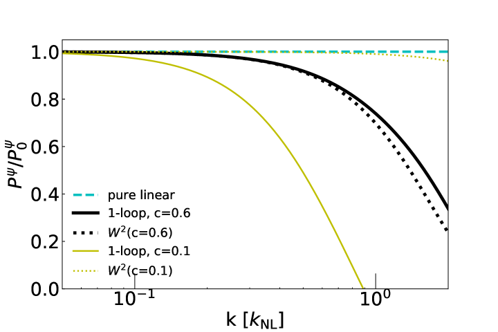
Figure 1: One loop suppression of displacement power, in 1D, for $n=2$. Dotted lines show the suppression of the linear power by $W(k)\equiv\exp\left(-k^{2}c^{2}/2\right)$, for the value of $c$ that sets the one loop correction to zero in the $k\rightarrow 0$ limit (black) or a smaller value for contrast (yellow), i.e., these are effectively truncated Zel’dovich, while the denominator is bare Zel’dovich. Solid adds the 1-loop correction, i.e., dotted is the leading order result and the difference between solid and dotted is the correction. For $n=2$ the correction in the $c\rightarrow 0$ limit is rapidly divergent. Note that the preferred $c$ is fixed entirely by the principle that the correction goes to zero in the low-$k$ limit—it is not a free parameter. In fact, we do not have simulations of the 1D displacement power, so the black curve is literally a (lowest order) prediction.

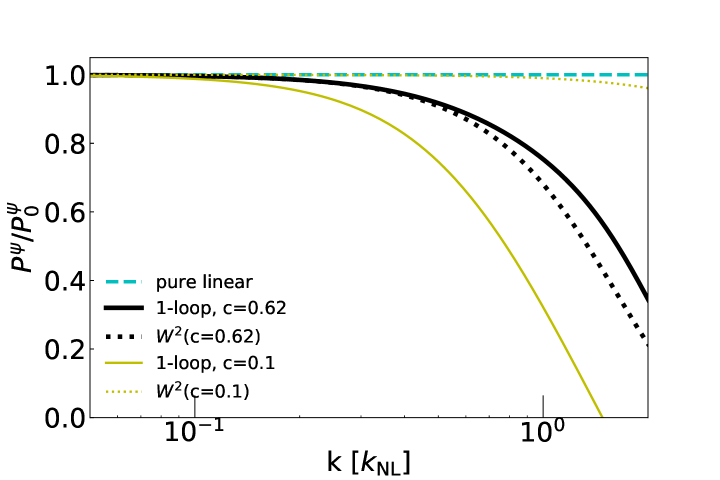
Figure 2: One loop suppression of displacement power, in 1D, for $n=1$, similar to Fig. 1.

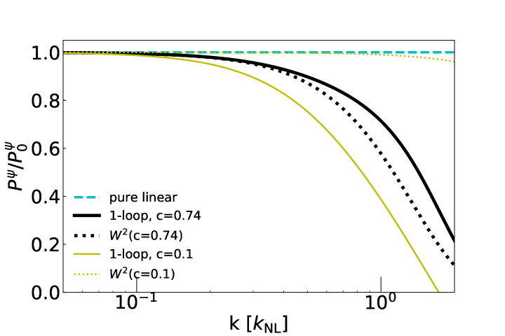
Figure 3: One loop suppression of displacement power, in 1D, for $n=0.5$, similar to Fig. 1.

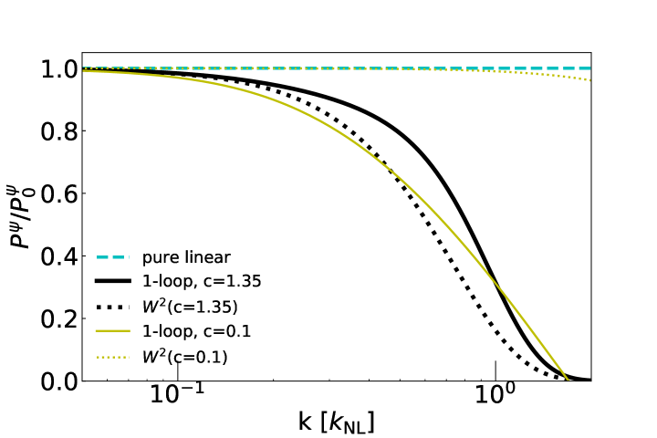
Figure 4: One loop suppression of displacement power, in 1D, for $n=0$.

A key thing to notice in these figures is the dependence of the power suppression on $c^{2}$. The larger value of $c^{2}$ results in less total suppression at 1-loop order, even though the direct leading order effect is more suppression. At small $c^{2}$, there is too much stream crossing at leading order, which leads to large 1-loop power suppression. The larger $c^{2}$ introduces an appropriate level of suppression at leading order, allowing 1-loop corrections to be small. Using an even larger value of $c^{2}$ than we plot here reverses the trend, giving leading order suppression too large so that the 1-loop correction must become large and positive to compensate.

This use of $W(k)$ with $c^{2}$ calibration is not the main point of the paper (in case it is not clear: it is not fundamentally related to the inclusion of stream crossing) so we defer most discussion to Sec. V, but we address a couple questions here. First note that, at least in this 1D calculation, $c^{2}$ is guaranteed to be positive, so we do not need to worry about $e^{-c^{2}k^{2}}$ diverging. As discussed below, we expect any serious 3D application to use an at least slightly more sophisticated replacement for the procedure used here, so there is no point in thinking about when the exact approach here might pathologically break down. Second, it would be very natural for $c^{2}$ to be time dependent, i.e., we would evaluate Eq. (37) at all $\eta$ instead of $\eta=0$. For an arbitrary power spectrum this would introduce significant complication as we would need to solve the matching for a continuous function, with values at a given time depending on all values in the past, but for power law EdS models we would still only need to solve for one number because we know exactly what the time dependence must be. The only scale in the problem is the nonlinear scale where $\Delta^{2}(k_{\rm NL})=1\propto e^{2\eta}k^{n+d}$, so $k_{\rm NL}(\eta)\propto e^{-2\eta/(n+d)}$ (assuming $n+d>0$). $c^{2}(\eta)$ must be $\propto k_{\rm NL}^{-2}(\eta)\propto e^{4\eta/(n+d)}$, with only the coefficient to be determined by matching. We expect that using this would make calculations at a given order more accurate by bringing the leading order closer to the truth, but it is important to understand that the calculation is mathematically consistent either way, because in either case the part that is taken away is restored as a perturbation. If we wanted to use a constant $c^{2}$ to make predictions in a model with arbitrary power spectrum, there would be nothing fundamentally wrong with simply computing a different value at each redshift we were interested in—in each case the fixed $c^{2}$ used in the calculation would represent a reasonable $\sim$time-averaged value for that redshift. There is certainly ambiguity here, but that is true of all perturbation theory, where the definition of orders is generally not unique—what we hope for is that the series we are computing converges to the same answer for any reasonable choice.

IV.2.4 Density power spectrum

The nontrivial density power spectrum contribution is

$$\left<\delta(\mathbf{k}_{1},\eta)\delta(\mathbf{k}_{2},\eta)\right>^{(a)}_{1} = \int d^{d}\mathbf{q}_{1}\int d^{d}\mathbf{q}_{2}~{}e^{i\mathbf{k}_{1}\cdot\mathbf{q}_{1}+i\mathbf{k}_{2}\cdot\mathbf{q}_{2}}e^{i\mathbf{k}_{1}\cdot\partial_{\mathbf{j}_{\mathbf{\psi}}(\mathbf{q}_{1},\eta)}+i\mathbf{k}_{2}\cdot\partial_{\mathbf{j}_{\mathbf{\psi}}(\mathbf{q}_{2},\eta)}}Z_{1}^{(a)}(\mathbf{j})\left.\right|_{\mathbf{j}=0}$$

$$= \frac{3}{2}(2\pi)^{d}\delta^{D}(\mathbf{k}_{1}+\mathbf{k}_{2})\int d^{d}\mathbf{q}_{12}d^{d}\mathbf{q}d\eta^{\prime}\int d^{d}\mathbf{q}^{\prime}\frac{d^{d}\mathbf{k}}{\left(2\pi\right)^{d}}\frac{\mathbf{k}\cdot\mathbf{L}^{-1}_{\psi\upsilon}\left(\mathbf{q}\right)\cdot\mathbf{k}_{1}}{k^{2}}e^{i\mathbf{k}_{1}\cdot\mathbf{q}_{12}}$$

$$\qquad\left[e^{i\mathbf{k}\cdot\mathbf{Q}\left(\mathbf{q},\mathbf{q}^{\prime},\eta^{\prime}\mathbf{q}_{12},\eta,\mathbf{k}_{1}\right)}-e^{-i\mathbf{k}\cdot\mathbf{Q}\left(\mathbf{q},\mathbf{q}^{\prime},\eta^{\prime}\mathbf{q}_{12},\eta,\mathbf{k}_{1}\right)}\right]e^{-\frac{1}{2}k_{i}\sigma^{2}_{ij}(\mathbf{q}^{\prime},\eta^{\prime})k_{j}}e^{-\frac{1}{2}k_{1i}\sigma^{2}_{ij}(\mathbf{q}_{12},\eta)k_{1j}}-{\rm mean~{}part}$$

where $\mathbf{Q}\left(\mathbf{q},\mathbf{q}^{\prime},\eta^{\prime}\mathbf{q}_{12},\eta,\mathbf{k}_{1}\right)\equiv\mathbf{q}^{\prime}-i\mathbf{\Xi}\left(\mathbf{q},\mathbf{q}^{\prime},\eta^{\prime},\mathbf{q}_{12},\eta\right)\cdot\mathbf{k}_{1}$ and

$$\mathbf{\Xi}(\mathbf{q},\mathbf{q}^{\prime},\eta^{\prime},\mathbf{q}_{12},\eta) \equiv \mathbf{C}_{\psi}(\mathbf{q},\eta^{\prime},\eta)-\mathbf{C}_{\psi}(\mathbf{q}+\mathbf{q}_{12},\eta^{\prime},\eta)-\mathbf{C}_{\psi}(\mathbf{q}+\mathbf{q}^{\prime},\eta^{\prime},\eta)+\mathbf{C}_{\psi}(\mathbf{q}+\mathbf{q}^{\prime}+\mathbf{q}_{12},\eta^{\prime},\eta)~{}.$$ (39)

In 1D we can again integrate over $k$:

$$\left<\delta(k_{1},\eta)\delta(k_{2},\eta)\right>^{(a),1D}_{1} = -(2\pi)\delta^{D}(k_{1}+k_{2})\frac{3}{2}{\rm Im}\int dq_{12}dqd\eta^{\prime}e^{ik_{1}q_{12}}\mathbf{L}^{-1}_{\psi\upsilon}(q,\eta,\eta^{\prime})$$

$$\qquad\qquad k_{1}\int dq^{\prime}{\rm erf}\left[\frac{q^{\prime}-ik_{1}\Xi(q,q^{\prime},\eta^{\prime},q_{12},\eta)}{\sqrt{2}\sigma\left(q^{\prime},\eta^{\prime}\right)}\right]e^{-\frac{1}{2}k_{1}^{2}\sigma^{2}(q_{12},\eta)}-{\rm mean~{}part}$$

The suppressed-power-restoring contribution to the density power spectrum is

$$\left<\delta(\mathbf{k}_{1},\eta)\delta(\mathbf{k}_{2},\eta)\right>^{(c)}_{1} = \int d^{d}\mathbf{q}_{1}\int d^{d}\mathbf{q}_{2}~{}e^{i\mathbf{k}_{1}\cdot\mathbf{q}_{1}+i\mathbf{k}_{2}\cdot\mathbf{q}_{2}}e^{i\mathbf{k}_{1}\partial_{\mathbf{j}_{\mathbf{\psi}}(\mathbf{q}_{1},\eta)}+i\mathbf{k}_{2}\partial_{\mathbf{j}_{\mathbf{\psi}}(\mathbf{q}_{2},\eta)}}\left[Z_{1}^{(c)}(\mathbf{j})-Z_{1}^{(c)}(0)Z_{0}(\mathbf{j})\right]\left.\right|_{\mathbf{j}=0}$$

$$= \int d^{d}\mathbf{q}_{1}\int d^{d}\mathbf{q}_{2}~{}e^{i\mathbf{k}_{1}\cdot\mathbf{q}_{1}+i\mathbf{k}_{2}\cdot\mathbf{q}_{2}}e^{i\mathbf{k}_{1}\partial_{\mathbf{j}_{\mathbf{\psi}}(\mathbf{q}_{1},\eta)}+i\mathbf{k}_{2}\partial_{\mathbf{j}_{\mathbf{\psi}}(\mathbf{q}_{2},\eta)}}\mathbf{j}^{t}\left(1-W\left(k\right)\right)\mathbf{C}\mathbf{j}~{}Z_{0}(\mathbf{j})\left.\right|_{\mathbf{j}=0}$$

$$= -(2\pi)\delta^{D}(k_{1}+k_{2})\int d^{d}\mathbf{q}~{}\cos\left(\mathbf{k}_{1}\cdot\mathbf{q}\right)~{}k^{m}_{1}\sigma_{1-W}^{2mn}(q,\eta)k^{n}_{1}~{}e^{-\frac{1}{2}k^{i}_{1}\sigma_{ij}^{2}(q,\eta)k^{j}_{1}}~{}.$$

So our final density power spectrum predictions are shown in Figs. 5-8.

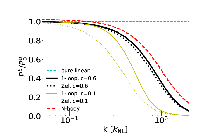
Figure 5: One loop density power, in 1D, for $n=2$, relative to the initial power law. Solid black shows the final one loop prediction, using the value of $c$ fixed internally by the displacement power calculation as shown in Fig. 1. Black dotted shows the Zel’dovich power for the same $c$, i.e., the difference is the happily small one loop correction. Red dashed are the N-body results of McQuinn and White (2016), who say that their $n=2$ simulations had not fully converged. E.g., the points at low $k$ are almost surely a couple percent lower where they would agree well with our prediction (see the smaller-$n$ figures that follow where they did not have this issue). For comparison, we show the same quantities for $c=0.1$, where the one loop calculation makes a valiant effort to correct the massive failure of Zel’dovich, but it is clear that $c=0.6$ is a much better starting point for a perturbative expansion.

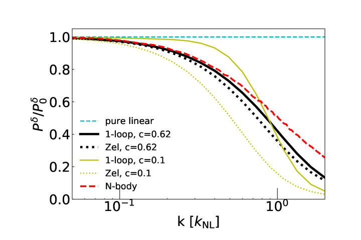
Figure 6: One loop density power, in 1D, for $n=1$, relative to the initial power law, similar to Fig. 5. Note that the values of $c$ used in all figures were computed literally “blind” to the simulation results—it was clear that $W(k)$ was needed to keep blue spectra from diverging (and from common-sense understanding of the physics), and the exact numerical values used here were settled by the displacement power calculation before the density power was ever computed.

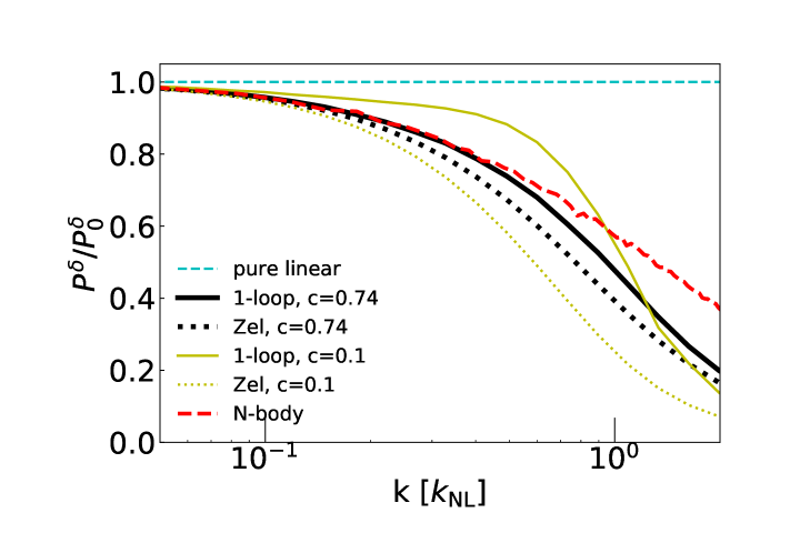
Figure 7: One loop density power, in 1D, for $n=0.5$, relative to the initial power law, similar to Fig. 5.

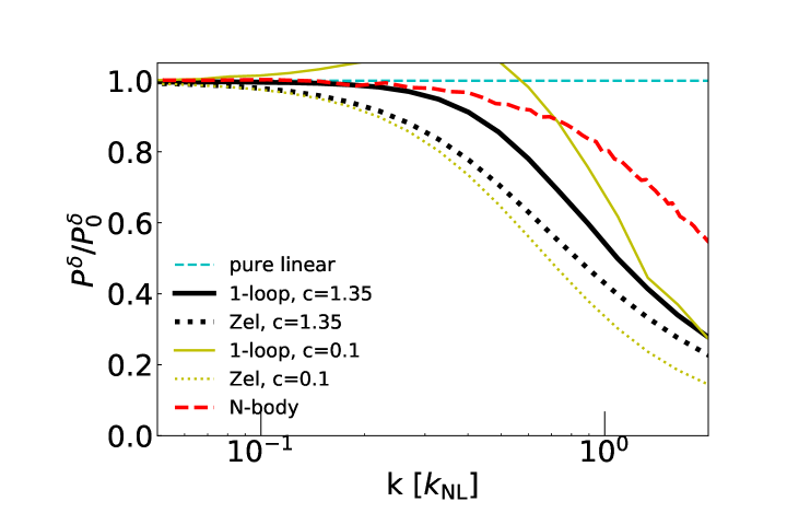
Figure 8: One loop density power, in 1D, for $n=0$, relative to the initial power law, similar to Fig. 5.

We see first that the numerical values of $c$ computed by setting the one loop correction to the low-$k$ displacement power to zero do a great job producing a perturbative expansion where the corrections are in fact small. This calibration is entirely internal to the theory. Even if we only had the Zel’dovich vs. corrected curves for density power here, it would be obvious that the calibrated values of $c$ are a lot better than significantly different ones, just based on the principle that higher order terms in a perturbative expansion should be small. Compared to the N-body results of McQuinn and White (2016), we see that the predictions for $n=1$ and $n=1/2$ are excellent at low $k$, breaking down at the 10% level at slightly higher $k$ than the free-parameter-fitted “EFT” curves shown in McQuinn and White (2016), and breaking down much more gracefully (in all cases gradually under-predicting the simulation power). The comparison for $n=2$ is murky because McQuinn and White (2016) had trouble achieving convergence in the simulations—in any case, considering that the naive Zel’dovich prediction is divergent for $n=2$, our theory seems like a very big step forward. Finally, $n=0$ presents a somewhat greater challenge for the theory. While we successfully predict that the power will only start deviating from linear at higher $k$ than Zel’dovich, we do not predict these deviations very well once they happen. It may be that this is because a Gaussian $W(k)$ is less appropriate for this spectrum with more low-$k$ power. We see in Fig. 4 that our kernel matched in the asymptotic low-$k$ limit is not doing a good job matching the predicted damping at higher $k$. This can be fixed by finding a kernel that matches the calculated suppression better. There are many other possible refinements of the leading order theory that might improve the results, discussed in Sec. V, but of course we may simply need another loop.

V Discussion

There are many obvious next steps for this formalism, e.g., computing displacement, density, etc. power spectra in 3D and comparing to numerical simulations Carlson et al. (2009); Tassev and Zaldarriaga (2012); Nishimichi et al. (2007); Nomura et al. (2008); Takahashi et al. (2008); Shoji et al. (2009); Nishimichi et al. (2009); Orban and Weinberg (2011), computing other statistics like the bispectrum Sefusatti and Komatsu (2007); Pan et al. (2007); Rampf and Buchert (2012); Baldauf et al. (2012); Rampf and Wong (2012); Lazanu et al. (2016); Hoffmann et al. (2017), or power spectrum covariance matrix Neyrinck and Szapudi (2008); Takahashi et al. (2009, 2011); Bertolini et al. (2016), etc. Efforts to speed up PT numerical evaluation Schmittfull et al. (2016); Schmittfull and Vlah (2016); McEwen et al. (2016); Fang et al. (2017); Simonović et al. (2017) could be reconsidered in this context. Here we discuss a few possibilities where we may have something useful to say about the path forward.

V.1 Non-Gaussianity, modified gravity, neutrinos, baryons, bias, redshift space distortions, etc.

It should not be too hard to fit primordial non-Gaussianity McDonald (2008); Bartolo et al. (2010); Giannantonio and Porciani (2010); Gong and Yokoyama (2011); Alvarez et al. (2014); Moradinezhad Dizgah and Dvorkin (2017) into this formalism. By definition the modification of the starting point statistical distribution for $\mathbf{\epsilon}$, Eq. (14), will add an extra non-Gaussian part to the perturbative piece $S_{p}$. Note that any kind of polynomial in $\phi\propto k^{-2}\delta$ can be constructed by repeated applications of the $\delta$-generating operator.

Typical modifications of gravity Taruya et al. (2014); Aviles and Cervantes-Cota (2017) should not present any new problem for this formalism. In standard perturbation theory, calculations are usually simplified by the good approximation for density statistics Takahashi (2008) that the growth at each order $n$ is proportional to $D^{n}(t)$, where $D(t)$ is the linear growth factor. This means, as far as density statistics is considered, we have not needed to do numerical time integrals as part of PT [other than to compute $D(t)$]. For momentum correlators this approximation starts to be less than percent accurate and corrections need to be taken into account Fasiello and Vlah (2016). In the calculations of this paper, however, we have abandoned this feature—time integration is an unavoidable part of the calculation including stream crossing. We also integrate over $k$-dependence of the propagator, which is not necessary in SPT. Having accepted these necessities, we can implement a modified gravity model that forces them on us with no additional complication. Non-linear effects can be included as perturbations.

Perturbation theory for massive neutrinos Lesgourgues et al. (2009); Saito et al. (2009); Führer and Wong (2015); Shoji and Komatsu (2010a, b) may be an ideal application for this formalism. The only practical difference at late times between neutrinos and cold dark matter amounts to initial conditions—the initial conditions for neutrinos include large velocities that are uncorrelated down to arbitrarily small scales. It should be possible to represent the neutrinos with a displacement field just like we have discussed for CDM by imagining a snapshot at some early time and defining $\mathbf{N}$ to give appropriate random velocities in addition to the usual initial correlated perturbations. The first calculation to do will be the displacement power spectrum to determine the small-scale suppression kernel $W(k)$ for the neutrinos, which will be appropriately longer range. The key point is: because the formalism already fully includes stream crossing, and deals gracefully with naively very large dispersion in the initial conditions (e.g., infinite for $n=2$ here), there should be no need for, e.g., special evolution equations for neutrinos. To be clear: we would now have separate $\mathbf{\psi}$ and $\mathbf{\upsilon}$ for the neutrinos, driven by the combined density field, with $\mathbf{L}$ becoming a $4\times 4$ matrix multiplying fields, etc.. To more faithfully represent all the relevant physics, this scenario may provide extra motivation for more detailed renormalization of $\mathbf{L}$ and renormalization of $\mathbf{N}$, as discussed below.

Unfortunately, what we have here is a theory for dark matter, which is not generally observable. Gravitational lensing Troxel et al. (2017); DES Collaboration et al. (2017); Bernstein et al. (2016); Jenkins et al. (2014); Zhan and Tyson (2017); Di Dio (2017); Madhavacheril et al. (2015) is typically cited as the most direct tracer, but even this is sensitive to baryon pressure effects on small-scales Eifler et al. (2015), and ultimately is an observation of galaxies (or some other source of photons), not directly mass, with corresponding biasing issues like intrinsic alignments Chisari and Dvorkin (2013); Krause et al. (2016); Blazek et al. (2017). Baryon displacement fields can easily be introduced to at least model the effect of the difference in initial conditions on large scales Ma and Bertschinger (1995); Hu and Sugiyama (1995); Seljak and Zaldarriaga (1996); Singh and Ma (2002); Yoshida et al. (2003); Tseliakhovich and Hirata (2010); Bernardeau et al. (2013). We could easily add explicit pressure terms for a given equation of state (this might be especially interesting for describing the Ly$\alpha$ forest McDonald et al. (2000, 2002); McDonald (2003); Afshordi et al. (2003); Mandelbaum et al. (2003); McDonald et al. (2005, 2006); McDonald and Eisenstein (2007), where little effort has been made to use higher order perturbation theory, even though its generally weak non-linearity would seem to make it a good candidate), but it is not clear that the perturbation theory as it stands will represent the physics fully correctly, because baryon streams should really never cross (they should shock instead), while the perturbation theory might effectively allow them to sometimes, at which point, e.g., the pressure force might be effectively pointing in the wrong direction. $W(k)$ the way we use it probably cannot entirely control this problem. It might be necessary to introduce something that more completely stops the possibility of crossing (e.g., Gurbatov et al. (1989); Kofman and Shandarin (1988); Weinberg and Gunn (1990); Valageas (2011)), although we would want to be sure that this was a controlled modification of the perturbative expansion like our $W(k)$, not an arbitrary hack. Another possibility might be to use Eulerian-type fields for baryons while still using displacements for dark matter, as in Eulerian hydrodynamic simulations Cen (1992); Bryan et al. (2014). While some kind of effective model with free or externally fixed parameters is inevitably needed for modeling temperatures any time they are affected by star formation or other complex physics, it would be interesting to see if any progress could be made including an explicit temperature field computed from a few simple principles to describe a relatively simple system like the IGM McDonald et al. (2001).

One of the most hopeful uses for perturbation theory is to organize our understanding of biasing models describing how galaxies and other observables trace dark matter McDonald and Roy (2009); Nishimichi and Oka (2014); Desjacques et al. (2016); Hand et al. (2017). The usual Eulerian bias prescriptions McDonald (2006); Smith et al. (2007); Jeong and Komatsu (2009); McDonald and Roy (2009); Chan and Scoccimarro (2012); Saito et al. (2014); Beutler et al. (2017); Ata et al. (2017) should be straightforward to implement in this formalism, with correlations involving powers of $\delta(\mathbf{x})$ and its derivatives computed by repeated applications of the $\delta$-generating operator. For Lagrangian bias Matsubara (2008b, 2011); Elia et al. (2011) we can always write some function of $\mathbf{\phi}(\mathbf{q})$ as a weight next to the delta function in Eq. (3), and the tracers will stream-cross just like dark matter.

Redshift space distortions Matsubara (2008b); McDonald and Seljak (2009); McDonald (2009); Taruya et al. (2009); Blake et al. (2010); Taruya et al. (2010); Matsubara (2011); Seljak and McDonald (2011); Okumura et al. (2012a, b); Vlah et al. (2012); Schlagenhaufer et al. (2012); Montesano et al. (2012); Okumura et al. (2014); Chuang et al. (2017) can be included for dark matter with no additional approximation. We just add the appropriate apparent radial displacement $\propto\mathbf{\upsilon}_{\parallel}$ in the exponential when constructing density fields. Redshift space distortions for tracers like galaxies are a little trickier because, while low-$k$ modes of velocity should be the same as dark matter, this is not generally true on smaller scales, so some kind of generalized biasing model is needed to allow for the full range of possibilities.

V.2 Deriving effective theories

Suppose that instead of statistics we really want a theory for the Eulerian field $\delta(\mathbf{x})$. We can introduce it into $Z$ using a delta function like this:

$$Z=\int d\mathbf{\delta}_{S}~{}d\mathbf{\phi}~{}d\mathbf{\chi}~{}\delta^{D}[\mathbf{\delta}_{S}-\mathbf{\delta}_{S}(\mathbf{\psi})]~{}e^{-S(\mathbf{\phi},\mathbf{\chi})}=\int d\mathbf{\delta}_{S}~{}d\mathbf{\pi}~{}d\mathbf{\phi}~{}d\mathbf{\chi}~{}e^{i\mathbf{\pi}^{t}\left[\mathbf{\delta}_{S}-\mathbf{\delta}_{S}(\mathbf{\psi})\right]-S(\mathbf{\phi},\mathbf{\chi})}~{},$$ (42)

where we have written $\mathbf{\delta}_{S}$ to indicate that we probably want to construct a theory for a smoothed version of $\mathbf{\delta}$. We can now substitute Eq. (4) for $\mathbf{\delta}(\mathbf{\psi})$ and if we can perform the integrals over $\mathbf{\phi}$ and $\mathbf{\chi}$ we will have a theory for $\mathbf{\delta}_{S}$, with $\mathbf{\pi}$ playing the role that $\mathbf{\chi}$ does for $\mathbf{\phi}$. We can perform these integrals perturbatively by pulling the standard linear approximation out of $\mathbf{\delta}(\mathbf{\psi})$ to write $\delta(\mathbf{k})=i\mathbf{k}\cdot\mathbf{\psi}(\mathbf{k})+...$ where the leading piece here will become part of the Gaussian integral over $\psi$ and the rest will be included in the perturbative part of the integration. I.e., we can achieve a generating function for $\mathbf{\delta}$ statistics that can be made increasingly accurate by including higher order perturbative integral contributions. The formula will be for $\delta(t)$, and so imply evolution equations (and initial conditions) which could be used in different ways. If the calculation is done consistently for smoothed $\delta_{S}$, the evolution equations will correctly represent dynamics entirely in terms of the smoothed fields. A similar calculation could be used to construct equations for other fields, e.g., moments of the velocity distribution function (momentum, energy, etc. McDonald (2011)) can easily be written as integrals like the one for $\mathbf{\delta}(\mathbf{\psi})$. One might ask “how likely is it that this could be an accurate theory, when it includes integration over small-scale $\mathbf{\phi}$?” That is not clear, but at least the size of perturbative terms will allow an internal estimate, and the $W(k)$-type suppression of small scales at leading order should aid convergence.

Another possibility, especially relevant if calculations in the full stream-crossing theory turn out to be slower than in traditional PT, would be to calibrate the free parameters of previous theories (e.g., Vlah et al. (2016)) by matching predictions to the stream crossing theory in the low-$k$ limit. It should be possible to make the matching step fast because formulas simplify in the low-$k$ limit.

V.3 More sophisticated renormalization

We intentionally tried to minimize the footprint of $W(k)$ in this paper, to avoid distracting from the main point about stream crossing, but clearly the issue it is addressing (of traditional linear theory being a terrible starting point for perturbation theory) is very generally important. Our approach here evolved from a more standard field theory starting point Peskin and Schroeder (1995). One of our original motivations was the observation that “EFT of LSS” proponents Baumann et al. (2012); Carrasco et al. (2012); Hertzberg (2014) did not seem to be taking their effective theory seriously enough, in that their prescription introduced terms intended to represent effective pressure/viscosity, but treated them as perturbations to the traditional fluid equations, rather than taking them seriously as part of the leading order linear evolution as one naturally would have done if given a system with these terms already in the linearized equations. This was presumably for ease of computation, but means that the terms can only be used to cancel potentially divergent parts of the higher order corrections, rather than prevent the divergence from ever happening as they probably physically should do. We originally thought to improve their treatment by fully including $k^{2}\delta$-type terms in $\mathbf{L}$ where they would naturally damp the propagator Blas et al. (2015); Rigopoulos (2015); Führer and Rigopoulos (2016). We thought to follow a standard Wilsonian RG procedure Wilson and Kogut (1974); Peskin and Schroeder (1995) of integrating out fields in shells of $\mathbf{k}$, absorbing the corrections into the coefficients of the effective theory. E.g., computing $\left<\mathbf{\chi}\mathbf{\phi}^{t}\right>$ perturbatively will give you corrections to $\mathbf{L}^{-1}$, which can then be disentangled from corrections to $\mathbf{N}$ in $\left<\mathbf{\phi}\mathbf{\phi}^{t}\right>$. Higher order interactions will also be generated. Because of the self-regulating nature of the propagator damping, i.e., that increasing a coefficient like $c^{2}$ generally decreases the calculated small-scale contribution to it, we expected to find $c^{2}$ values like we obtained here as some sort of fixed points of the RG evolution. At some point we realized that this full procedure might not be necessary—that we could capture the most relevant physics in the simpler way presented here. (We tell this historical story because it is helpful to understand the relation between our approach and standard field theory approaches.) A natural thought at this point would be “ok, what you have is a poor-person’s version of the full Wilsonian treatment, so a next step must be to more fully implement that.” But it is not clear that this is correct—it may be that, for our problem, standard field theory renormalization should be seen as the poor-person’s version of what we do here. Renormalization in quantum field theory takes the form it does because of the infinities that are apparently unavoidable in the calculations, i.e., where we had an equation like $c^{2}=f(c)$ to solve, they have $c^{2}=f(c)+\infty$. Obviously solving this directly is no good, so they go on to observe that the derivative of $c^{2}$ with respect to some matching point (like our $k\rightarrow 0$) or similarly the contribution from integrating out a small shell of $\mathbf{k}$ in the Wilsonian picture, is finite. This allows them to calculate how $c^{2}$ changes with scale (where note that here we are using $c^{2}$ abstractly to represent any parameter, like a particle mass), but the initial condition for this running is still corrupted by the infinity and must be treated as a free parameter. The possible exception to this problem is if the parameter hits a fixed point of the RG evolution, so it acquires a value independent of the initial conditions, but this generally does not happen for all parameters. If we do not have any true deep-UV sensitivity in our system, i.e., do not have any divergence once enough correct physics is included for the system to self-regulate, we can hope to avoid free parameters, solving for parameters of the Gaussian model as we have done here for $c^{2}$ instead of only computing relative values between different scales. From the conventional point of view this is probably equivalent to saying all parameters flow to a fixed point. If this sounds like wishful thinking, note that we implicitly take for granted that it is possible to construct an effective theory of dark matter clustering that has no free parameters, while being finite and completely insensitive to small-scale degrees of freedom. We use this theory all the time: N-body simulations, where we generally take for granted that larger scale structure converges as the numerical resolution increases.

There is another reason to prefer the approach we use to more literally pursuing the Wilsonian picture of integrating out shells of modes: in those calculations, generally the integration results in a contribution that cannot be represented by a convenient, small number of terms in the Lagrangian (equivalent to terms in our $S$), so one is forced to “truncate the basis,” i.e., ignore some of the calculation that does not project onto the terms you want to track. This is a potential source of error, not necessarily easy to control, which we avoid in our approach here where we do not throw anything away. Maybe the two approaches can be combined somehow—if nothing else, the exercise of integrating out small scale modes should help to identify and understand the useful modifications of the expansion.

Our modification of $\mathbf{L}^{-1}$ by a single overall suppression function $W(k)$ with semiarbitrarily chosen Gaussian form was intended to absolutely minimally capture what are of course really more complicated effects. While the details should be filled in by higher order terms, this should be more efficient if the leading order model can be improved. The first extension one might make is to allow for separate $\mathbf{\psi}\mathbf{\psi}$, $\mathbf{\psi}\mathbf{\upsilon}$, and $\mathbf{\upsilon}\mathbf{\upsilon}$ kernels. While there is always a temptation to judge the value of this kind of detail based on whether it appears to improve agreement with simulations, this is really not necessary—these differences are an inevitable consequence of computing all the elements of $\left<\mathbf{\phi}\mathbf{\phi}^{t}\right>$ and $\left<\mathbf{\phi}\mathbf{\chi}^{t}\right>$, and can be calibrated entirely internally, i.e., if we compute something other than the $\left<\mathbf{\psi}\mathbf{\psi}^{t}\right>$ that we computed here, using $c^{2}$ from $\left<\mathbf{\psi}\mathbf{\psi}^{t}\right>$, we would find a less perfect match. By making $W(k)$ a matrix in $(\mathbf{\psi},\mathbf{\upsilon})$, we can match all terms in $\left<\mathbf{\phi}\mathbf{\phi}^{t}\right>$ at once. More generally, we should also match $\left<\mathbf{\phi}\mathbf{\chi}^{t}\right>$, which is more directly identified with $\mathbf{L}^{-1}$, while $\left<\mathbf{\phi}\mathbf{\phi}^{t}\right>$ is also sensitive to, and therefore can be used to make corrections to, the noise $\mathbf{N}$. The noise modifications should presumably be additive instead of multiplicative and go like $k^{4}$ at low $k$ Peebles (1980). We could also attempt to match computed corrections to higher $k$ by modifying the form of $W(k)$ [and similarly $\delta N(k)$ if using it]. Similarly, these modifications are generally matrices in time, which can be calibrated in more detail by evaluating unequal time correlations. Also similarly, in higher dimensions $W(k)$ could be generalized to be asymmetric depending on the relation between its vector indices and $\mathbf{q}/\mathbf{k}$ (like the dependence of $C_{\psi_{i}\psi_{j}}(\mathbf{q})$ on whether the indices are along or transverse to $\mathbf{q}$). In other words: ultimately $\mathbf{L}^{-1}$ and $\mathbf{N}$ are general matrices in the full relevant space, and one could imagine working to make all loop corrections to them zero. Note, however, that we should not think that each new correction absorbed will make the final predictions more accurate by the full amount absorbed—once the corrections are small enough to take the form of a rapidly converging series, it should not matter much if they are absorbed at lowest order or computed perturbatively. To identify non-Gaussian terms, it will probably be useful to perform a large/small scale split of the fields, perturbatively integrate out the small scale part, and see how to interpret the result as a modification of the large-scale equations (this would also tell us how to modify the Gaussian part, if we could not guess).

We tried to keep our $W(k)$ calibration simple by including the contribution to changing $P_{\psi}$ from all scales, but, especially if we were isolating $\mathbf{L}^{-1}$ by computing $\left<\mathbf{\phi}\mathbf{\chi}^{t}\right>$, we might encounter an issue known in more standard perturbation theory, that very large scale bulk flows can make significant (even divergent) contributions to matching calculations like we did here even though their effect on smaller, observation-scale fluctuations is not actually to damp them. In fact, for an asymptotically large-scale flow there should be no effect at all, by Galilean invariance. Even very large scale stream crossing will not necessarily have a simple damping effect on smaller scale fluctuations within the flow (it seems there will be a change in background density, plus noise from the uncorrelated fluctuations in the other stream, but not the direct damping you get from displacements streaming out of their own driving perturbations). If this is found to be an issue, it will probably be useful in the future to do something like splitting the fields into a small and large scale contribution, basically relative to the scale of observation, and only including the contribution from the small-scale part when modifying $\mathbf{L}^{-1}$. Because we are not permanently throwing anything away in these calculations, only shifting some of the naive Gaussian part of the functional integral into the perturbative part, the results should not be very sensitive to, e.g., where exactly you put the large/small split.

Finally, note that some attempts to implement Wilsonian RG Matarrese and Pietroni (2007); Izumi and Soda (2007); Matarrese and Pietroni (2008); Floerchinger et al. (2017) ideas have been criticized for only integrating out small-scale fluctuations in the initial conditions, not in the evolving fields Rosten (2008). It is clear in the formalism presented here how one could integrate these fluctuations out of all fields at all times.

We thank Matt McQuinn for the N-body results from McQuinn and White (2016), and Anže Slosar and Zack Slepian for helpful comments on drafts.

Z.V. is supported in part by the U.S. Department of Energy contract to SLAC no. DE-AC02-76SF00515.

Appendix A Pedagogical explanation of the key math trick

The very simple math trick that makes this paper work may not be easy to identify within the formalism of our calculations, so we attempt to explain it more pedagogically here. Standard perturbation theory amounts to repeatedly performing the following type of integral:

$$\int dx~{}e^{-\frac{1}{2}x^{2}+jx-\lambda x^{3}+...}=\int dx~{}e^{-\frac{1}{2}x^{2}+jx}\left(1-\lambda x^{3}+...\right)$$ (43)

i.e., it is based on the fact that one kind of integral we can do analytically is a Gaussian times a polynomial. If some more general function of $x$ appears in the exponential here, one’s first instinct is to Taylor expand it to obtain a polynomial. However, we observe that we can also do

$$\int dx~{}e^{-\frac{1}{2}x^{2}+jx-\lambda e^{\alpha x}+...}=\int dx~{}e^{-\frac{1}{2}x^{2}+jx}\left(1-\lambda e^{\alpha x}+...\right)=\int dx~{}e^{-\frac{1}{2}x^{2}+jx}-\lambda e^{-\frac{1}{2}x^{2}+(j+\alpha)x}+...$$ (44)

i.e., if the coefficients of the Gaussian include exponentials, we can simply absorb them back into the Gaussian and again do the integral analytically. In the main calculation in this paper the formula for density as exponential in displacement, Eq. (4), is analogous to $e^{\alpha x}$ here. We avoid losing stream crossing by not Taylor expanding $e^{i\mathbf{k}\cdot\mathbf{\psi}}$ (which is tempting because it gives us a polynomial in $\mathbf{\psi}$), but instead expanding this whole exponential factor out of the $e^{-S}$ exponential and doing the calculation in the way of Eq. (44). The “action of the derivative operator” that leads to Eq. (IV.2.1) amounts to, underneath all the notation, an integration over force derived from density written in terms of exponentiated displacement. This is the key to the new result.

Appendix B Jacobian of $\mathbf{\epsilon}\rightarrow\mathbf{\phi}$ variable change

Our evaluation of the Jacobian determinant factor in the change of variables from $\mathbf{\epsilon}$ to $\phi$ follows similar calculations done in Valageas (2001, 2007a).

$${\rm det}\left(\frac{\partial\mathbf{\epsilon}}{\partial\mathbf{\phi}}\right)={\rm det}\left(\mathbf{L}_{0}+\frac{\partial\mathbf{\Delta}_{0}(\mathbf{\phi})}{\partial\mathbf{\phi}}\right)={\rm det}\left(\mathbf{L}_{0}\right){\rm det}\left(\mathbf{I}+\mathbf{L}_{0}^{-1}\frac{\partial\mathbf{\Delta}_{0}(\mathbf{\phi})}{\partial\mathbf{\phi}}\right)\propto e^{{\rm Tr}\ln\left(\mathbf{I}+\mathbf{L}_{0}^{-1}\mathbf{M}\right)}$$ (45)

where we have dropped the obviously field-independent ${\rm det}\left(\mathbf{L}_{0}\right)$, defined $\mathbf{M}\equiv\frac{\partial\mathbf{\Delta}_{0}}{\partial\mathbf{\phi}}$, and used the identity ${\rm det}\mathbf{A}=e^{{\rm Tr}\ln\mathbf{A}}$. Note that $\mathbf{\Delta}_{0}$ has only an $\mathbf{\upsilon}$ component, but only depends on $\mathbf{\psi}$, which means that in $\mathbf{M}$ only $\mathbf{M}_{\mathbf{\upsilon}\mathbf{\psi}}$ is non-zero. Taylor expanding in $\mathbf{L}_{0}^{-1}\mathbf{M}$ gives

$${\rm Tr}\ln\left(\mathbf{I}+\mathbf{L}_{0}^{-1}\mathbf{M}\right)=-\sum_{n=1}^{\infty}\frac{1}{n}{\rm Tr}\left[\left(-\mathbf{L}_{0}^{-1}\mathbf{M}\right)^{n}\right]~{}.$$ (46)

All of these terms take the form ${\rm Tr}\left[\mathbf{L}^{-1}_{0\mathbf{\psi}\mathbf{\upsilon}}\mathbf{M}_{\mathbf{\upsilon}\mathbf{\psi}}\mathbf{L}^{-1}_{0\mathbf{\psi}\mathbf{\upsilon}}\mathbf{M}_{\mathbf{\upsilon}\mathbf{\psi}}...\right]$. With $\mathbf{M}$ a delta function and $\mathbf{L}_{0}^{-1}$ a Heaviside function in the difference between their time indices, we see that the trace, which requires time to flow in a circle, i.e., $\int dt_{1}dt_{2}...dt_{n}A(t_{1},t_{2})...A(t_{n},t_{1})$, must give zero except possibly for the tricky limit where all times are the same so all $\Theta$ functions are evaluated at zero (with one integral over time remaining). For a general evolution equation, we would need a more subtle analysis of the equal time limit, but here it is simple because $\mathbf{L}^{-1}_{0\mathbf{\psi}\mathbf{\upsilon}}(\eta,\eta)=0$ independent of the $\Theta$ function, so every term is unambiguously zero.

B.1 Alternative derivation

We learned a different way to derive our basic functional integral starting point from Bartelmann et al. (2016). Starting from the likelihood function for $\mathbf{\epsilon}$, Eq. (14), we can enforce the evolution Eq. (9) using a delta function:

$$Z(\mathbf{j})=\int~{}d\mathbf{\phi}~{}d\mathbf{\epsilon}~{}\delta^{D}\left[\mathbf{\phi}-\mathbf{\phi}\left(\mathbf{\epsilon}\right)\right]~{}e^{-\frac{1}{2}\mathbf{\epsilon}^{t}\mathbf{N}^{-1}\mathbf{\epsilon}}\propto\int~{}d\mathbf{\phi}~{}d\mathbf{\epsilon}~{}\delta^{D}\left[\mathbf{\epsilon}-\mathbf{\epsilon}\left(\mathbf{\phi}\right)\right]~{}e^{-\frac{1}{2}\mathbf{\epsilon}^{t}\mathbf{N}^{-1}\mathbf{\epsilon}}=\int d\mathbf{\phi}~{}d\mathbf{\epsilon}~{}d\mathbf{\chi}~{}e^{i\mathbf{\chi}^{t}\left[\mathbf{\epsilon}-\mathbf{\epsilon}\left(\mathbf{\phi}\right)\right]-\frac{1}{2}\mathbf{\epsilon}^{t}\mathbf{N}^{-1}\mathbf{\epsilon}}$$ (47)

where we have used the same fact that the Jacobian of the $\mathbf{\epsilon}$-$\mathbf{\phi}$ transformation is field independent to change arguments in the delta function. Note that this transformation is invertible, e.g., if we imagine discretizing the evolution equation, it is easy to see that knowing $\mathbf{\epsilon}$ uniquely determines $\mathbf{\phi}$ and vice versa (this is easier than inverting a final field to determine initial conditions—here we know the field at all times by definition). We can now insert Eq. (9) for $\mathbf{\epsilon}(\mathbf{\phi})$ and perform the Gaussian integral over $\mathbf{\epsilon}$ to obtain Eq. (18-19). $\chi$ plays a role enforcing the evolution equation instead of appearing through an apparently arbitrary Gaussian integral trick.

Appendix C Low-$k$ expansion of density power formula

We can consider a small $k$ expansion of the erf part of Eq. (IV.2.4). For small $y$, ${\rm erf}(x+iy)={\rm erf}(x)+2iy\exp\left(-x^{2}\right)/\sqrt{\pi}+...$. The leading term gives zero in the $q^{\prime}$ integral, so we have:

$$-\frac{3}{2}{\rm Im}\int dq_{12}dqd\eta^{\prime}e^{ik_{1}q_{12}}\mathbf{L}^{-1}_{\psi\upsilon}(q,\eta,\eta^{\prime})k_{1}\int dq^{\prime}{\rm erf}\left[\frac{q^{\prime}-ik_{1}\Xi(q,q^{\prime},\eta^{\prime},q_{12},\eta)}{\sqrt{2}\sigma\left(q^{\prime},\eta^{\prime}\right)}\right]e^{-\frac{1}{2}k_{1}^{2}\sigma^{2}(q_{12},\eta)}$$ (48)

$$\simeq 3k_{1}^{2}\int dq_{12}dqd\eta^{\prime}\cos\left(k_{1}q_{12}\right)\mathbf{L}^{-1}_{\psi\upsilon}(q,\eta,\eta^{\prime})\int dq^{\prime}\Xi(q,q^{\prime},\eta^{\prime},q_{12},\eta)G\left[q^{\prime},\sigma\left(q^{\prime},\eta^{\prime}\right)\right]e^{-\frac{1}{2}k_{1}^{2}\sigma^{2}(q_{12},\eta)}$$

$$\simeq 3k_{1}^{2}\int dq_{12}\cos\left(k_{1}q_{12}\right)e^{-\frac{1}{2}k_{1}^{2}\sigma^{2}(q_{12},\eta)}\int d\eta^{\prime}[\mathbf{L}^{-1}_{0}]_{\psi\upsilon}(\eta,\eta^{\prime})\int dq^{\prime}\Xi_{W}(0,q^{\prime},\eta^{\prime},q_{12},\eta)G\left[q^{\prime},\sigma\left(q^{\prime},\eta^{\prime}\right)\right]$$

where in the last line we note that the $q$ integral is a convolution between $W(q)$ in $\mathbf{L}^{-1}$ and $\Xi$ and remove the $q$ integral by defining $\Xi_{W}$ to be $\Xi$ with the power spectrum used to compute it multiplied by an extra factor of $W(k)$.

For the 1D cases we have tried, we find that, while the approximation is valid at low enough $k$, “low enough” is always too low to be useful.

References

- Bernardeau et al. (2002) F. Bernardeau, S. Colombi, E. Gaztanaga, and R. Scoccimarro, “Large-scale structure of the Universe and cosmological perturbation theory.” Phys. Rept. 367, 1–128 (2002).
- Font-Ribera et al. (2014) A. Font-Ribera, P. McDonald, N. Mostek, B. A. Reid, H.-J. Seo, and A. Slosar, “DESI and other Dark Energy experiments in the era of neutrino mass measurements,” JCAP 5, 023 (2014), arXiv:1308.4164 .
- DESI Collaboration et al. (2016) DESI Collaboration, A. Aghamousa, J. Aguilar, S. Ahlen, S. Alam, L. E. Allen, C. Allende Prieto, J. Annis, S. Bailey, C. Balland, and et al., “The DESI Experiment Part I: Science,Targeting, and Survey Design,” ArXiv e-prints (2016), arXiv:1611.00036 [astro-ph.IM] .
- Zel’Dovich (1970) Y. B. Zel’Dovich, “Gravitational instability: an approximate theory for large density perturbations.” Astron. Astrophys. 5, 84–89 (1970).
- Davis et al. (1985) M. Davis, G. Efstathiou, C. S. Frenk, and S. D. M. White, “The evolution of large-scale structure in a universe dominated by cold dark matter,” Astrophys. J. 292, 371–394 (1985).
- Feng et al. (2016) Y. Feng, M.-Y. Chu, U. Seljak, and P. McDonald, “FASTPM: a new scheme for fast simulations of dark matter and haloes,” Mon. Not. Roy. Astron. Soc. 463, 2273–2286 (2016), arXiv:1603.00476 .
- Buchert and Ehlers (1993) T. Buchert and J. Ehlers, “Lagrangian theory of gravitational instability of Friedman-Lemaitre cosmologies – second-order approach: an improved model for non-linear clustering,” Mon. Not. Roy. Astron. Soc. 264, 375–387 (1993).
- Bouchet et al. (1995) F. R. Bouchet, S. Colombi, E. Hivon, and R. Juszkiewicz, “Perturbative Lagrangian approach to gravitational instability.” Astron. Astrophys. 296, 575–+ (1995), astro-ph/9406013 .
- Matsubara (2008a) T. Matsubara, “Resumming cosmological perturbations via the Lagrangian picture: One-loop results in real space and in redshift space,” Phys. Rev. D 77, 063530–+ (2008a), arXiv:0711.2521 .
- Okamura et al. (2011) T. Okamura, A. Taruya, and T. Matsubara, “Next-to-leading resummation of cosmological perturbations via the Lagrangian picture: 2-loop correction in real and redshift spaces,” JCAP 8, 012 (2011), arXiv:1105.1491 [astro-ph.CO] .
- Rampf (2012) C. Rampf, “The recursion relation in Lagrangian perturbation theory,” JCAP 12, 004 (2012), arXiv:1205.5274 [astro-ph.CO] .
- Vlah et al. (2015) Z. Vlah, U. Seljak, and T. Baldauf, “Lagrangian perturbation theory at one loop order: Successes, failures, and improvements,” Phys. Rev. D 91, 023508 (2015), arXiv:1410.1617 .
- Peebles (1980) P. J. E. Peebles, The large-scale structure of the universe (Research supported by the National Science Foundation. Princeton, N.J., Princeton University Press, 1980. 435 p., 1980).
- Goroff et al. (1986) M. H. Goroff, B. Grinstein, S.-J. Rey, and M. B. Wise, “Coupling of modes of cosmological mass density fluctuations,” Astrophys. J. 311, 6–14 (1986).
- McDonald (2011) P. McDonald, “How to generate a significant effective temperature for cold dark matter, from first principles,” JCAP 4, 32–+ (2011), arXiv:0910.1002 [astro-ph.CO] .
- McDonald (2007) P. McDonald, “Dark matter clustering: A simple renormalization group approach,” Phys. Rev. D 75, 043514–+ (2007).
- McDonald (2014) P. McDonald, “What the ”simple renormalization group” approach to dark matter clustering really was,” ArXiv e-prints (2014), arXiv:1403.7235 .
- Taruya and Hiramatsu (2008) A. Taruya and T. Hiramatsu, “A Closure Theory for Nonlinear Evolution of Cosmological Power Spectra,” Astrophys. J. 674, 617–635 (2008), arXiv:0708.1367 .
- Afshordi (2007) N. Afshordi, “How well can (renormalized) perturbation theory predict dark matter clustering properties?” Phys. Rev. D 75, 021302–+ (2007), arXiv:astro-ph/0610336 .
- Pueblas and Scoccimarro (2009) S. Pueblas and R. Scoccimarro, “Generation of vorticity and velocity dispersion by orbit crossing,” Phys. Rev. D 80, 043504–+ (2009), arXiv:0809.4606 .
- Davis and Peebles (1977) M. Davis and P. J. E. Peebles, “On the integration of the BBGKY equations for the development of strongly nonlinear clustering in an expanding universe,” ApJS 34, 425–450 (1977).
- Tassev (2011) S. V. Tassev, “The Helmholtz Hierarchy: phase space statistics of cold dark matter,” JCAP 10, 022 (2011), arXiv:1012.0282 [astro-ph.CO] .
- Gurbatov et al. (1989) S. N. Gurbatov, A. I. Saichev, and S. F. Shandarin, “The large-scale structure of the universe in the frame of the model equation of non-linear diffusion,” Mon. Not. Roy. Astron. Soc. 236, 385–402 (1989).
- Kofman and Shandarin (1988) L. A. Kofman and S. F. Shandarin, “Theory of adhesion for the large-scale structure of the universe,” Nature (London) 334, 129–131 (1988).
- Weinberg and Gunn (1990) D. H. Weinberg and J. E. Gunn, “Largescale Structure and the Adhesion Approximation,” Mon. Not. Roy. Astron. Soc. 247, 260 (1990).
- Pietroni et al. (2012) M. Pietroni, G. Mangano, N. Saviano, and M. Viel, “Coarse-grained cosmological perturbation theory,” JCAP 1, 019 (2012), arXiv:1108.5203 [astro-ph.CO] .
- Baumann et al. (2012) D. Baumann, A. Nicolis, L. Senatore, and M. Zaldarriaga, “Cosmological non-linearities as an effective fluid,” JCAP 7, 051 (2012), arXiv:1004.2488 [astro-ph.CO] .
- Carrasco et al. (2012) J. J. M. Carrasco, M. P. Hertzberg, and L. Senatore, “The effective field theory of cosmological large scale structures,” Journal of High Energy Physics 9, 82 (2012), arXiv:1206.2926 [astro-ph.CO] .
- Hertzberg (2014) M. P. Hertzberg, “Effective field theory of dark matter and structure formation: Semianalytical results,” Phys. Rev. D 89, 043521 (2014).
- Aviles (2016) A. Aviles, “Dark matter dispersion tensor in perturbation theory,” Phys. Rev. D 93, 063517 (2016), arXiv:1512.07198 .
- Couchman and Bond (1988) H. M. P. Couchman and J. R. Bond, “Models for the evolution of the two point correlation function,” in Post-Recombination Universe, edited by N. Kaiser and A. N. Lasenby (1988) pp. 263–265.
- Valageas (2011) P. Valageas, “Impact of shell crossing and scope of perturbative approaches, in real and redshift space,” Astron. Astrophys. 526, A67 (2011), arXiv:1009.0106 .
- Valageas (2001) P. Valageas, “Dynamics of gravitational clustering. I. Building perturbative expansions,” Astron. Astrophys. 379, 8–20 (2001).
- Valageas (2002) P. Valageas, “Dynamics of gravitational clustering. II. Steepest-descent method for the quasi-linear regime,” Astron. Astrophys. 382, 412–430 (2002), astro-ph/0107126 .
- Valageas (2004) P. Valageas, “A new approach to gravitational clustering: A path-integral formalism and large-N expansions,” Astron. Astrophys. 421, 23–40 (2004), astro-ph/0307008 .
- Valageas (2007a) P. Valageas, “Large-N expansions applied to gravitational clustering,” Astron. Astrophys. 465, 725–747 (2007a), astro-ph/0611849 .
- Matarrese and Pietroni (2007) S. Matarrese and M. Pietroni, “Resumming cosmic perturbations,” Journal of Cosmology and Astro-Particle Physics 6, 26–+ (2007), arXiv:astro-ph/0703563 .
- Valageas (2007b) P. Valageas, “Using the Zeldovich dynamics to test expansion schemes,” Astron. Astrophys. 476, 31–58 (2007b), arXiv:0706.2593 .
- Valageas (2008) P. Valageas, “Expansion schemes for gravitational clustering: computing two-point and three-point functions,” Astron. Astrophys. 484, 79–101 (2008), arXiv:0711.3407 .
- Skovbo (2012) K. Skovbo, “Large-k limit of multi-point propagators in the RG formalism,” JCAP 3, 031 (2012), arXiv:1110.2655 [astro-ph.CO] .
- Rigopoulos (2015) G. Rigopoulos, “The adhesion model as a field theory for cosmological clustering,” JCAP 1, 014 (2015), arXiv:1404.7283 .
- Führer and Rigopoulos (2016) F. Führer and G. Rigopoulos, “Renormalizing a viscous fluid model for large scale structure formation,” JCAP 2, 032 (2016), arXiv:1509.03073 .
- Bartelmann et al. (2016) M. Bartelmann, F. Fabis, D. Berg, E. Kozlikin, R. Lilow, and C. Viermann, “A microscopic, non-equilibrium, statistical field theory for cosmic structure formation,” New Journal of Physics 18, 043020 (2016).
- Ali-Haïmoud (2015) Y. Ali-Haïmoud, “Perturbative interaction approach to cosmological structure formation,” Phys. Rev. D 91, 103507 (2015), arXiv:1502.00580 .
- Taruya and Colombi (2017) A. Taruya and S. Colombi, “Post-collapse perturbation theory in 1D cosmology - beyond shell-crossing,” Mon. Not. Roy. Astron. Soc. 470, 4858–4884 (2017), arXiv:1701.09088 .
- Crocce and Scoccimarro (2006a) M. Crocce and R. Scoccimarro, “Memory of initial conditions in gravitational clustering,” Phys. Rev. D 73, 063520–+ (2006a).
- Crocce and Scoccimarro (2006b) M. Crocce and R. Scoccimarro, “Renormalized cosmological perturbation theory,” Phys. Rev. D 73, 063519–+ (2006b).
- Crocce and Scoccimarro (2008) M. Crocce and R. Scoccimarro, “Nonlinear evolution of baryon acoustic oscillations,” Phys. Rev. D 77, 023533–+ (2008), arXiv:0704.2783 .
- Bernardeau and Valageas (2008) F. Bernardeau and P. Valageas, “Propagators in Lagrangian space,” Phys. Rev. D 78, 083503–+ (2008), arXiv:0805.0805 .
- Bernardeau et al. (2008) F. Bernardeau, M. Crocce, and R. Scoccimarro, “Multipoint propagators in cosmological gravitational instability,” Phys. Rev. D 78, 103521–+ (2008), arXiv:0806.2334 .
- Anselmi et al. (2011) S. Anselmi, S. Matarrese, and M. Pietroni, “Next-to-leading resummations in cosmological perturbation theory,” JCAP 6, 015 (2011), arXiv:1011.4477 [astro-ph.CO] .
- Taruya et al. (2012) A. Taruya, F. Bernardeau, T. Nishimichi, and S. Codis, “Direct and fast calculation of regularized cosmological power spectrum at two-loop order,” Phys. Rev. D 86, 103528 (2012), arXiv:1208.1191 [astro-ph.CO] .
- Sugiyama and Futamase (2012) N. S. Sugiyama and T. Futamase, “An Application of the Wiener Hermite Expansion to the Nonlinear Evolution of Dark Matter,” Astrophys. J. 760, 114 (2012), arXiv:1210.1663 [astro-ph.CO] .
- Bernardeau et al. (2012) F. Bernardeau, M. Crocce, and R. Scoccimarro, “Constructing regularized cosmic propagators,” Phys. Rev. D 85, 123519 (2012), arXiv:1112.3895 [astro-ph.CO] .
- McQuinn and White (2016) M. McQuinn and M. White, “Cosmological perturbation theory in 1+1 dimensions,” JCAP 1, 043 (2016), arXiv:1502.07389 .
- Wilson and Kogut (1974) K. G. Wilson and J. Kogut, “The renormalization group and the expansion,” Phys. Rept. 12, 75–199 (1974).
- Hubbard (1959) J. Hubbard, “Calculation of Partition Functions,” Physical Review Letters 3, 77–78 (1959).
- Stratonovich (1957) R. L. Stratonovich, “On a Method of Calculating Quantum Distribution Functions,” Soviet Physics Doklady 2, 416 (1957).
- Martin et al. (1973) P. C. Martin, E. D. Siggia, and H. A. Rose, “Statistical Dynamics of Classical Systems,” Phys. Rev. A 8, 423–437 (1973).
- Phythian (1977) R. Phythian, “The functional formalism of classical statistical dynamics,” Journal of Physics A Mathematical General 10, 777–789 (1977).
- Taylor and Hamilton (1996) A. N. Taylor and A. J. S. Hamilton, “Non-linear cosmological power spectra in real and redshift space,” Mon. Not. Roy. Astron. Soc. 282, 767–778 (1996), astro-ph/9604020 .
- Doroshkevich et al. (1973) A. G. Doroshkevich, V. S. Ryaben’kii, and S. F. Shandarin, “Nonlinear theory of the development of potential perturbations,” Astrophysics 9, 144–153 (1973).
- Blas et al. (2015) D. Blas, S. Floerchinger, M. Garny, N. Tetradis, and U. A. Wiedemann, “Large scale structure from viscous dark matter,” JCAP 11, 049 (2015), arXiv:1507.06665 .
- Carlson et al. (2009) J. Carlson, M. White, and N. Padmanabhan, “Critical look at cosmological perturbation theory techniques,” Phys. Rev. D 80, 043531–+ (2009), arXiv:0905.0479 .
- Tassev and Zaldarriaga (2012) S. Tassev and M. Zaldarriaga, “The mildly non-linear regime of structure formation,” JCAP 4, 013 (2012), arXiv:1109.4939 .
- Nishimichi et al. (2007) T. Nishimichi, H. Ohmuro, M. Nakamichi, A. Taruya, K. Yahata, A. Shirata, S. Saito, H. Nomura, K. Yamamoto, and Y. Suto, “Characteristic Scales of Baryon Acoustic Oscillations from Perturbation Theory: Nonlinearity and Redshift-Space Distortion Effects,” PASJ 59, 1049– (2007), arXiv:0705.1589 .
- Nomura et al. (2008) H. Nomura, K. Yamamoto, and T. Nishimichi, “Damping of the baryon acoustic oscillations in the matter power spectrum as a probe of the growth factor,” JCAP 10, 031 (2008), arXiv:0809.4538 .
- Takahashi et al. (2008) R. Takahashi, N. Yoshida, T. Matsubara, N. Sugiyama, I. Kayo, T. Nishimichi, A. Shirata, A. Taruya, S. Saito, K. Yahata, and Y. Suto, “Simulations of baryon acoustic oscillations - I. Growth of large-scale density fluctuations,” Mon. Not. Roy. Astron. Soc. 389, 1675–1682 (2008), arXiv:0802.1808 .
- Shoji et al. (2009) M. Shoji, D. Jeong, and E. Komatsu, “Extracting Angular Diameter Distance and Expansion Rate of the Universe From Two-Dimensional Galaxy Power Spectrum at High Redshifts: Baryon Acoustic Oscillation Fitting Versus Full Modeling,” Astrophys. J. 693, 1404–1416 (2009), arXiv:0805.4238 .
- Nishimichi et al. (2009) T. Nishimichi, A. Shirata, A. Taruya, K. Yahata, S. Saito, Y. Suto, R. Takahashi, N. Yoshida, T. Matsubara, N. Sugiyama, I. Kayo, Y. Jing, and K. Yoshikawa, “Modeling Nonlinear Evolution of Baryon Acoustic Oscillations: Convergence Regime of N-body Simulations and Analytic Models,” PASJ 61, 321– (2009), arXiv:0810.0813 .
- Orban and Weinberg (2011) C. Orban and D. H. Weinberg, “Self-similar bumps and wiggles: Isolating the evolution of the BAO peak with power-law initial conditions,” Phys. Rev. D 84, 063501 (2011), arXiv:1101.1523 [astro-ph.CO] .
- Sefusatti and Komatsu (2007) E. Sefusatti and E. Komatsu, “Bispectrum of galaxies from high-redshift galaxy surveys: Primordial non-Gaussianity and nonlinear galaxy bias,” Phys. Rev. D 76, 083004–+ (2007), arXiv:0705.0343 .
- Pan et al. (2007) J. Pan, P. Coles, and I. Szapudi, “Scale transformations, tree-level perturbation theory and the cosmological matter bispectrum,” Mon. Not. Roy. Astron. Soc. 382, 1460–1464 (2007), arXiv:0707.1594 .
- Rampf and Buchert (2012) C. Rampf and T. Buchert, “Lagrangian perturbations and the matter bispectrum I: fourth-order model for non-linear clustering,” JCAP 6, 021 (2012), arXiv:1203.4260 [astro-ph.CO] .
- Baldauf et al. (2012) T. Baldauf, U. Seljak, V. Desjacques, and P. McDonald, “Evidence for quadratic tidal tensor bias from the halo bispectrum,” Phys. Rev. D 86, 083540 (2012), arXiv:1201.4827 [astro-ph.CO] .
- Rampf and Wong (2012) C. Rampf and Y. Y. Y. Wong, “Lagrangian perturbations and the matter bispectrum II: the resummed one-loop correction to the matter bispectrum,” JCAP 6, 018 (2012), arXiv:1203.4261 [astro-ph.CO] .
- Lazanu et al. (2016) A. Lazanu, T. Giannantonio, M. Schmittfull, and E. P. S. Shellard, “Matter bispectrum of large-scale structure: Three-dimensional comparison between theoretical models and numerical simulations,” Phys. Rev. D 93, 083517 (2016), arXiv:1510.04075 .
- Hoffmann et al. (2017) K. Hoffmann, E. Gaztanaga, R. Scoccimarro, and M. Crocce, “Testing the consistency of three-point halo clustering in Fourier and configuration space,” ArXiv e-prints (2017), arXiv:1708.08941 .
- Neyrinck and Szapudi (2008) M. C. Neyrinck and I. Szapudi, “Baryon oscillations in galaxy and matter power-spectrum covariance matrices,” Mon. Not. Roy. Astron. Soc. 384, 1221–1230 (2008), arXiv:0710.3586 .
- Takahashi et al. (2009) R. Takahashi, N. Yoshida, M. Takada, T. Matsubara, N. Sugiyama, I. Kayo, A. J. Nishizawa, T. Nishimichi, S. Saito, and A. Taruya, “Simulations of Baryon Acoustic Oscillations. II. Covariance Matrix of the Matter Power Spectrum,” Astrophys. J. 700, 479–490 (2009), arXiv:0902.0371 [astro-ph.CO] .
- Takahashi et al. (2011) R. Takahashi, N. Yoshida, M. Takada, T. Matsubara, N. Sugiyama, I. Kayo, T. Nishimichi, S. Saito, and A. Taruya, “Non-Gaussian Error Contribution to Likelihood Analysis of the Matter Power Spectrum,” Astrophys. J. 726, 7 (2011), arXiv:0912.1381 [astro-ph.CO] .
- Bertolini et al. (2016) D. Bertolini, K. Schutz, M. P. Solon, J. R. Walsh, and K. M. Zurek, “Non-Gaussian covariance of the matter power spectrum in the effective field theory of large scale structure,” Phys. Rev. D 93, 123505 (2016), arXiv:1512.07630 .
- Schmittfull et al. (2016) M. Schmittfull, Z. Vlah, and P. McDonald, “Fast large scale structure perturbation theory using one-dimensional fast Fourier transforms,” Phys. Rev. D 93, 103528 (2016), arXiv:1603.04405 .
- Schmittfull and Vlah (2016) M. Schmittfull and Z. Vlah, “Reducing the two-loop large-scale structure power spectrum to low-dimensional, radial integrals,” Phys. Rev. D 94, 103530 (2016), arXiv:1609.00349 .
- McEwen et al. (2016) J. E. McEwen, X. Fang, C. M. Hirata, and J. A. Blazek, “FAST-PT: a novel algorithm to calculate convolution integrals in cosmological perturbation theory,” JCAP 9, 015 (2016), arXiv:1603.04826 .
- Fang et al. (2017) X. Fang, J. A. Blazek, J. E. McEwen, and C. M. Hirata, “FAST-PT II: an algorithm to calculate convolution integrals of general tensor quantities in cosmological perturbation theory,” JCAP 2, 030 (2017), arXiv:1609.05978 .
- Simonović et al. (2017) M. Simonović, T. Baldauf, M. Zaldarriaga, J. J. Carrasco, and J. A. Kollmeier, “Cosmological Perturbation Theory Using the FFTLog: Formalism and Connection to QFT Loop Integrals,” ArXiv e-prints (2017), arXiv:1708.08130 .
- McDonald (2008) P. McDonald, “Primordial non-Gaussianity: Large-scale structure signature in the perturbative bias model,” Phys. Rev. D 78, 123519–+ (2008), arXiv:0806.1061 .
- Bartolo et al. (2010) N. Bartolo, J. P. Beltrán Almeida, S. Matarrese, M. Pietroni, and A. Riotto, “Signatures of primordial non-Gaussianities in the matter power-spectrum and bispectrum: the time-RG approach,” JCAP 3, 011 (2010), arXiv:0912.4276 [astro-ph.CO] .
- Giannantonio and Porciani (2010) T. Giannantonio and C. Porciani, “Structure formation from non-Gaussian initial conditions: Multivariate biasing, statistics, and comparison with N-body simulations,” Phys. Rev. D 81, 063530 (2010), arXiv:0911.0017 [astro-ph.CO] .
- Gong and Yokoyama (2011) J.-O. Gong and S. Yokoyama, “Scale-dependent bias from primordial non-Gaussianity with trispectrum,” Mon. Not. Roy. Astron. Soc. 417, L79–L82 (2011), arXiv:1106.4404 [astro-ph.CO] .
- Alvarez et al. (2014) M. Alvarez, T. Baldauf, J. R. Bond, N. Dalal, R. de Putter, O. Doré, D. Green, C. Hirata, Z. Huang, D. Huterer, D. Jeong, M. C. Johnson, E. Krause, M. Loverde, J. Meyers, P. D. Meerburg, L. Senatore, S. Shandera, E. Silverstein, A. Slosar, K. Smith, M. Zaldarriaga, V. Assassi, J. Braden, A. Hajian, T. Kobayashi, G. Stein, and A. van Engelen, “Testing Inflation with Large Scale Structure: Connecting Hopes with Reality,” ArXiv e-prints (2014), arXiv:1412.4671 .
- Moradinezhad Dizgah and Dvorkin (2017) A. Moradinezhad Dizgah and C. Dvorkin, “Scale-Dependent Galaxy Bias from Massive Particles with Spin during Inflation,” ArXiv e-prints (2017), arXiv:1708.06473 .
- Taruya et al. (2014) A. Taruya, T. Nishimichi, F. Bernardeau, T. Hiramatsu, and K. Koyama, “Regularized cosmological power spectrum and correlation function in modified gravity models,” Phys. Rev. D 90, 123515 (2014), arXiv:1408.4232 .
- Aviles and Cervantes-Cota (2017) A. Aviles and J. L. Cervantes-Cota, “A Lagrangian perturbation theory for modify gravity,” ArXiv e-prints (2017), arXiv:1705.10719 .
- Takahashi (2008) R. Takahashi, “Third-Order Density Perturbation and One-Loop Power Spectrum in Dark-Energy-Dominated Universe,” Progress of Theoretical Physics 120, 549–559 (2008), arXiv:0806.1437 .
- Fasiello and Vlah (2016) M. Fasiello and Z. Vlah, “Nonlinear fields in generalized cosmologies,” Phys. Rev. D 94, 063516 (2016), arXiv:1604.04612 .
- Lesgourgues et al. (2009) J. Lesgourgues, S. Matarrese, M. Pietroni, and A. Riotto, “Non-linear power spectrum including massive neutrinos: the time-RG flow approach,” Journal of Cosmology and Astro-Particle Physics 6, 17–+ (2009), arXiv:0901.4550 .
- Saito et al. (2009) S. Saito, M. Takada, and A. Taruya, “Nonlinear power spectrum in the presence of massive neutrinos: Perturbation theory approach, galaxy bias, and parameter forecasts,” Phys. Rev. D 80, 083528 (2009), arXiv:0907.2922 [astro-ph.CO] .
- Führer and Wong (2015) F. Führer and Y. Y. Y. Wong, “Higher-order massive neutrino perturbations in large-scale structure,” JCAP 3, 046 (2015), arXiv:1412.2764 .
- Shoji and Komatsu (2010a) M. Shoji and E. Komatsu, “Massive neutrinos in cosmology: Analytic solutions and fluid approximation,” Phys. Rev. D 81, 123516 (2010a).
- Shoji and Komatsu (2010b) M. Shoji and E. Komatsu, “Erratum: Massive neutrinos in cosmology: Analytic solutions and fluid approximation [Phys. Rev. D 81, 123516 (2010)],” Phys. Rev. D 82, 089901 (2010b), arXiv:1003.0942 [astro-ph.CO] .
- Troxel et al. (2017) M. A. Troxel, N. MacCrann, J. Zuntz, T. F. Eifler, E. Krause, S. Dodelson, D. Gruen, J. Blazek, O. Friedrich, S. Samuroff, J. Prat, L. F. Secco, C. Davis, A. Ferté, J. DeRose, A. Alarcon, A. Amara, E. Baxter, M. R. Becker, G. M. Bernstein, S. L. Bridle, R. Cawthon, C. Chang, A. Choi, J. De Vicente, A. Drlica-Wagner, J. Elvin-Poole, J. Frieman, M. Gatti, W. G. Hartley, K. Honscheid, B. Hoyle, E. M. Huff, D. Huterer, B. Jain, M. Jarvis, T. Kacprzak, D. Kirk, N. Kokron, C. Krawiec, O. Lahav, A. R. Liddle, J. Peacock, M. M. Rau, A. Refregier, R. P. Rollins, E. Rozo, E. S. Rykoff, C. Sánchez, I. Sevilla-Noarbe, E. Sheldon, A. Stebbins, T. N. Varga, P. Vielzeuf, M. Wang, R. H. Wechsler, B. Yanny, T. M. C. Abbott, F. B. Abdalla, S. Allam, J. Annis, K. Bechtol, A. Benoit-Lévy, E. Bertin, D. Brooks, E. Buckley-Geer, D. L. Burke, A. Carnero Rosell, M. Carrasco Kind, J. Carretero, F. J. Castander, M. Crocce, C. E. Cunha, C. B. D’Andrea, L. N. da Costa, D. L. DePoy, S. Desai, H. T. Diehl, J. P. Dietrich, P. Doel, E. Fernandez, B. Flaugher, P. Fosalba, J. García-Bellido, E. Gaztanaga, D. W. Gerdes, T. Giannantonio, D. A. Goldstein, R. A. Gruendl, J. Gschwend, G. Gutierrez, D. J. James, T. Jeltema, M. W. G. Johnson, M. D. Johnson, S. Kent, K. Kuehn, S. Kuhlmann, N. Kuropatkin, T. S. Li, M. Lima, H. Lin, M. A. G. Maia, M. March, J. L. Marshall, P. Martini, P. Melchior, F. Menanteau, R. Miquel, J. J. Mohr, E. Neilsen, R. C. Nichol, B. Nord, D. Petravick, A. A. Plazas, A. K. Romer, A. Roodman, M. Sako, E. Sanchez, V. Scarpine, R. Schindler, M. Schubnell, M. Smith, R. C. Smith, M. Soares-Santos, F. Sobreira, E. Suchyta, M. E. C. Swanson, G. Tarle, D. Thomas, D. L. Tucker, V. Vikram, A. R. Walker, J. Weller, and Y. Zhang, “Dark Energy Survey Year 1 Results: Cosmological Constraints from Cosmic Shear,” ArXiv e-prints (2017), arXiv:1708.01538 .
- DES Collaboration et al. (2017) DES Collaboration, T. M. C. Abbott, F. B. Abdalla, A. Alarcon, J. Aleksić, S. Allam, S. Allen, A. Amara, J. Annis, J. Asorey, S. Avila, D. Bacon, E. Balbinot, M. Banerji, N. Banik, W. Barkhouse, M. Baumer, E. Baxter, K. Bechtol, M. R. Becker, A. Benoit-Lévy, B. A. Benson, G. M. Bernstein, E. Bertin, J. Blazek, S. L. Bridle, D. Brooks, D. Brout, E. Buckley-Geer, D. L. Burke, M. T. Busha, D. Capozzi, A. Carnero Rosell, M. Carrasco Kind, J. Carretero, F. J. Castander, R. Cawthon, C. Chang, N. Chen, M. Childress, A. Choi, C. Conselice, R. Crittenden, M. Crocce, C. E. Cunha, C. B. D’Andrea, L. N. da Costa, R. Das, T. M. Davis, C. Davis, J. De Vicente, D. L. DePoy, J. DeRose, S. Desai, H. T. Diehl, J. P. Dietrich, S. Dodelson, P. Doel, A. Drlica-Wagner, T. F. Eifler, A. E. Elliott, F. Elsner, J. Elvin-Poole, J. Estrada, A. E. Evrard, Y. Fang, E. Fernandez, A. Ferté, D. A. Finley, B. Flaugher, P. Fosalba, O. Friedrich, J. Frieman, J. García-Bellido, M. Garcia-Fernandez, M. Gatti, E. Gaztanaga, D. W. Gerdes, T. Giannantonio, M. S. S. Gill, K. Glazebrook, D. A. Goldstein, D. Gruen, R. A. Gruendl, J. Gschwend, G. Gutierrez, S. Hamilton, W. G. Hartley, S. R. Hinton, K. Honscheid, B. Hoyle, D. Huterer, B. Jain, D. J. James, M. Jarvis, T. Jeltema, M. D. Johnson, M. W. G. Johnson, T. Kacprzak, S. Kent, A. G. Kim, A. King, D. Kirk, N. Kokron, A. Kovacs, E. Krause, C. Krawiec, A. Kremin, K. Kuehn, S. Kuhlmann, N. Kuropatkin, F. Lacasa, O. Lahav, T. S. Li, A. R. Liddle, C. Lidman, M. Lima, H. Lin, N. MacCrann, M. A. G. Maia, M. Makler, M. Manera, M. March, J. L. Marshall, P. Martini, R. G. McMahon, P. Melchior, F. Menanteau, R. Miquel, V. Miranda, D. Mudd, J. Muir, A. Möller, E. Neilsen, R. C. Nichol, B. Nord, P. Nugent, R. L. C. Ogando, A. Palmese, J. Peacock, H. V. Peiris, J. Peoples, W. J. Percival, D. Petravick, A. A. Plazas, A. Porredon, J. Prat, A. Pujol, M. M. Rau, A. Refregier, P. M. Ricker, N. Roe, R. P. Rollins, A. K. Romer, A. Roodman, R. Rosenfeld, A. J. Ross, E. Rozo, E. S. Rykoff, M. Sako, A. I. Salvador, S. Samuroff, C. Sánchez, E. Sanchez, B. Santiago, V. Scarpine, R. Schindler, D. Scolnic, L. F. Secco, S. Serrano, I. Sevilla-Noarbe, E. Sheldon, R. C. Smith, M. Smith, J. Smith, M. Soares-Santos, F. Sobreira, E. Suchyta, G. Tarle, D. Thomas, M. A. Troxel, D. L. Tucker, B. E. Tucker, S. A. Uddin, T. N. Varga, P. Vielzeuf, V. Vikram, A. K. Vivas, A. R. Walker, M. Wang, R. H. Wechsler, J. Weller, W. Wester, R. C. Wolf, B. Yanny, F. Yuan, A. Zenteno, B. Zhang, Y. Zhang, and J. Zuntz, “Dark Energy Survey Year 1 Results: Cosmological Constraints from Galaxy Clustering and Weak Lensing,” ArXiv e-prints (2017), arXiv:1708.01530 .
- Bernstein et al. (2016) G. M. Bernstein, R. Armstrong, C. Krawiec, and M. C. March, “An accurate and practical method for inference of weak gravitational lensing from galaxy images,” Mon. Not. Roy. Astron. Soc. 459, 4467–4484 (2016), arXiv:1508.05655 [astro-ph.IM] .
- Jenkins et al. (2014) E. E. Jenkins, A. V. Manohar, W. J. Waalewijn, and A. P. S. Yadav, “Higher-order gravitational lensing reconstruction using Feynman diagrams,” JCAP 9, 024 (2014), arXiv:1403.4607 .
- Zhan and Tyson (2017) H. Zhan and J. A. Tyson, “Cosmology with the Large Synoptic Survey Telescope,” ArXiv e-prints (2017), arXiv:1707.06948 .
- Di Dio (2017) E. Di Dio, “Lensing smoothing of BAO wiggles,” JCAP 3, 016 (2017), arXiv:1609.09044 .
- Madhavacheril et al. (2015) M. S. Madhavacheril, P. McDonald, N. Sehgal, and A. Slosar, “Building unbiased estimators from non-Gaussian likelihoods with application to shear estimation,” JCAP 1, 022 (2015), arXiv:1407.1906 .
- Eifler et al. (2015) T. Eifler, E. Krause, S. Dodelson, A. R. Zentner, A. P. Hearin, and N. Y. Gnedin, “Accounting for baryonic effects in cosmic shear tomography: determining a minimal set of nuisance parameters using PCA,” Mon. Not. Roy. Astron. Soc. 454, 2451–2471 (2015), arXiv:1405.7423 .
- Chisari and Dvorkin (2013) N. E. Chisari and C. Dvorkin, “Cosmological information in the intrinsic alignments of luminous red galaxies,” JCAP 12, 029 (2013), arXiv:1308.5972 [astro-ph.CO] .
- Krause et al. (2016) E. Krause, T. Eifler, and J. Blazek, “The impact of intrinsic alignment on current and future cosmic shear surveys,” Mon. Not. Roy. Astron. Soc. 456, 207–222 (2016), arXiv:1506.08730 .
- Blazek et al. (2017) J. Blazek, N. MacCrann, M. A. Troxel, and X. Fang, “Beyond linear galaxy alignments,” ArXiv e-prints (2017), arXiv:1708.09247 .
- Ma and Bertschinger (1995) C. Ma and E. Bertschinger, “Cosmological Perturbation Theory in the Synchronous and Conformal Newtonian Gauges,” Astrophys. J. 455, 7–+ (1995).
- Hu and Sugiyama (1995) W. Hu and N. Sugiyama, “Anisotropies in the cosmic microwave background: an analytic approach,” Astrophys. J. 444, 489–506 (1995).
- Seljak and Zaldarriaga (1996) U. Seljak and M. Zaldarriaga, “A line-of-sight integration approach to cosmic microwave background anisotropies,” Astrophys. J. 469, 437–444 (1996).
- Singh and Ma (2002) S. Singh and C.-P. Ma, “Linear and Second-Order Evolution of Cosmic Baryon Perturbations below 106 Solar Masses,” Astrophys. J. 569, 1–7 (2002), astro-ph/0111450 .
- Yoshida et al. (2003) N. Yoshida, N. Sugiyama, and L. Hernquist, “The evolution of baryon density fluctuations in multicomponent cosmological simulations,” Mon. Not. Roy. Astron. Soc. 344, 481–491 (2003), astro-ph/0305210 .
- Tseliakhovich and Hirata (2010) D. Tseliakhovich and C. Hirata, “Relative velocity of dark matter and baryonic fluids and the formation of the first structures,” Phys. Rev. D 82, 083520 (2010), arXiv:1005.2416 .
- Bernardeau et al. (2013) F. Bernardeau, N. Van de Rijt, and F. Vernizzi, “Power spectra in the eikonal approximation with adiabatic and nonadiabatic modes,” Phys. Rev. D 87, 043530 (2013), arXiv:1209.3662 [astro-ph.CO] .
- McDonald et al. (2000) P. McDonald, J. Miralda-Escudé, M. Rauch, W. L. W. Sargent, T. A. Barlow, R. Cen, and J. P. Ostriker, “The Observed Probability Distribution Function, Power Spectrum, and Correlation Function of the Transmitted Flux in the Ly Forest,” Astrophys. J. 543, 1–23 (2000).
- McDonald et al. (2002) P. McDonald, J. Miralda-Escudé, and R. Cen, “Large-Scale Correlation of Mass and Galaxies with the Ly Forest Transmitted Flux,” Astrophys. J. 580, 42–53 (2002).
- McDonald (2003) P. McDonald, “Toward a Measurement of the Cosmological Geometry at z ~ 2: Predicting Ly Forest Correlation in Three Dimensions and the Potential of Future Data Sets,” Astrophys. J. 585, 34–51 (2003), arXiv:astro-ph/0108064 .
- Afshordi et al. (2003) N. Afshordi, P. McDonald, and D. N. Spergel, “Primordial Black Holes as Dark Matter: The Power Spectrum and Evaporation of Early Structures,” Astrophys. J. Let. 594, L71–L74 (2003).
- Mandelbaum et al. (2003) R. Mandelbaum, P. McDonald, U. Seljak, and R. Cen, “Precision cosmology from the Lyman- forest: power spectrum and bispectrum,” Mon. Not. Roy. Astron. Soc. 344, 776–788 (2003).
- McDonald et al. (2005) P. McDonald, U. Seljak, R. Cen, D. Shih, D. H. Weinberg, S. Burles, D. P. Schneider, D. J. Schlegel, N. A. Bahcall, J. W. Briggs, J. Brinkmann, M. Fukugita, Ž. Ivezić, S. Kent, and D. E. Vanden Berk, “The Linear Theory Power Spectrum from the Ly Forest in the Sloan Digital Sky Survey,” Astrophys. J. 635, 761–783 (2005).
- McDonald et al. (2006) P. McDonald, U. Seljak, S. Burles, D. J. Schlegel, D. H. Weinberg, R. Cen, D. Shih, J. Schaye, D. P. Schneider, N. A. Bahcall, J. W. Briggs, J. Brinkmann, R. J. Brunner, M. Fukugita, J. E. Gunn, Ž. Ivezić, S. Kent, R. H. Lupton, and D. E. Vanden Berk, “The Ly Forest Power Spectrum from the Sloan Digital Sky Survey,” ApJS 163, 80–109 (2006), arXiv:astro-ph/0405013 .
- McDonald and Eisenstein (2007) P. McDonald and D. J. Eisenstein, “Dark energy and curvature from a future baryonic acoustic oscillation survey using the Lyman- forest,” Phys. Rev. D 76, 063009–+ (2007), arXiv:astro-ph/0607122 .
- Cen (1992) R. Cen, “A hydrodynamic approach to cosmology - Methodology,” ApJS 78, 341–364 (1992).
- Bryan et al. (2014) G. L. Bryan, M. L. Norman, B. W. O’Shea, T. Abel, J. H. Wise, M. J. Turk, D. R. Reynolds, D. C. Collins, P. Wang, S. W. Skillman, B. Smith, R. P. Harkness, J. Bordner, J.-h. Kim, M. Kuhlen, H. Xu, N. Goldbaum, C. Hummels, A. G. Kritsuk, E. Tasker, S. Skory, C. M. Simpson, O. Hahn, J. S. Oishi, G. C. So, F. Zhao, R. Cen, Y. Li, and Enzo Collaboration, “ENZO: An Adaptive Mesh Refinement Code for Astrophysics,” ApJS 211, 19 (2014), arXiv:1307.2265 [astro-ph.IM] .
- McDonald et al. (2001) P. McDonald, J. Miralda-Escudé, M. Rauch, W. L. W. Sargent, T. A. Barlow, and R. Cen, “A Measurement of the Temperature-Density Relation in the Intergalactic Medium Using a New Ly Absorption-Line Fitting Method,” Astrophys. J. 562, 52–75 (2001).
- McDonald and Roy (2009) P. McDonald and A. Roy, “Clustering of dark matter tracers: generalizing bias for the coming era of precision LSS,” JCAP 8, 020 (2009), arXiv:0902.0991 [astro-ph.CO] .
- Nishimichi and Oka (2014) T. Nishimichi and A. Oka, “Simulating the anisotropic clustering of luminous red galaxies with subhaloes: a direct confrontation with observation and cosmological implications,” Mon. Not. Roy. Astron. Soc. 444, 1400–1418 (2014), arXiv:1310.2672 .
- Desjacques et al. (2016) V. Desjacques, D. Jeong, and F. Schmidt, “Large-Scale Galaxy Bias,” ArXiv e-prints (2016), arXiv:1611.09787 .
- Hand et al. (2017) N. Hand, U. Seljak, F. Beutler, and Z. Vlah, “Extending the modeling of the anisotropic galaxy power spectrum to ,” ArXiv e-prints (2017), arXiv:1706.02362 .
- McDonald (2006) P. McDonald, “Clustering of dark matter tracers: Renormalizing the bias parameters,” Phys. Rev. D 74, 103512–+ (2006).
- Smith et al. (2007) R. E. Smith, R. Scoccimarro, and R. K. Sheth, “Scale dependence of halo and galaxy bias: Effects in real space,” Phys. Rev. D 75, 063512–+ (2007), arXiv:astro-ph/0609547 .
- Jeong and Komatsu (2009) D. Jeong and E. Komatsu, “Perturbation Theory Reloaded. II. Nonlinear Bias, Baryon Acoustic Oscillations, and Millennium Simulation in Real Space,” Astrophys. J. 691, 569–595 (2009), arXiv:0805.2632 .
- Chan and Scoccimarro (2012) K. C. Chan and R. Scoccimarro, “Halo sampling, local bias, and loop corrections,” Phys. Rev. D 86, 103519 (2012), arXiv:1204.5770 [astro-ph.CO] .
- Saito et al. (2014) S. Saito, T. Baldauf, Z. Vlah, U. Seljak, T. Okumura, and P. McDonald, “Understanding higher-order nonlocal halo bias at large scales by combining the power spectrum with the bispectrum,” Phys. Rev. D 90, 123522 (2014), arXiv:1405.1447 .
- Beutler et al. (2017) F. Beutler, H.-J. Seo, A. J. Ross, P. McDonald, S. Saito, A. S. Bolton, J. R. Brownstein, C.-H. Chuang, A. J. Cuesta, D. J. Eisenstein, A. Font-Ribera, J. N. Grieb, N. Hand, F.-S. Kitaura, C. Modi, R. C. Nichol, W. J. Percival, F. Prada, S. Rodriguez-Torres, N. A. Roe, N. P. Ross, S. Salazar-Albornoz, A. G. Sánchez, D. P. Schneider, A. Slosar, J. Tinker, R. Tojeiro, M. Vargas-Magaña, and J. A. Vazquez, “The clustering of galaxies in the completed SDSS-III Baryon Oscillation Spectroscopic Survey: baryon acoustic oscillations in the Fourier space,” Mon. Not. Roy. Astron. Soc. 464, 3409–3430 (2017), arXiv:1607.03149 .
- Ata et al. (2017) M. Ata, F.-S. Kitaura, C.-H. Chuang, S. Rodríguez-Torres, R. E. Angulo, S. Ferraro, H. Gil-Marín, P. McDonald, C. Hernández Monteagudo, V. Müller, G. Yepes, M. Autefage, F. Baumgarten, F. Beutler, J. R. Brownstein, A. Burden, D. J. Eisenstein, H. Guo, S. Ho, C. McBride, M. Neyrinck, M. D. Olmstead, N. Padmanabhan, W. J. Percival, F. Prada, G. Rossi, A. G. Sánchez, D. Schlegel, D. P. Schneider, H.-J. Seo, A. Streblyanska, J. Tinker, R. Tojeiro, and M. Vargas-Magana, “The clustering of galaxies in the completed SDSS-III Baryon Oscillation Spectroscopic Survey: cosmic flows and cosmic web from luminous red galaxies,” Mon. Not. Roy. Astron. Soc. 467, 3993–4014 (2017), arXiv:1605.09745 .
- Matsubara (2008b) T. Matsubara, “Nonlinear perturbation theory with halo bias and redshift-space distortions via the Lagrangian picture,” Phys. Rev. D 78, 083519–+ (2008b).
- Matsubara (2011) T. Matsubara, “Nonlinear perturbation theory integrated with nonlocal bias, redshift-space distortions, and primordial non-Gaussianity,” Phys. Rev. D 83, 083518 (2011), arXiv:1102.4619 [astro-ph.CO] .
- Elia et al. (2011) A. Elia, S. Kulkarni, C. Porciani, M. Pietroni, and S. Matarrese, “Modelling the clustering of dark matter haloes in resummed perturbation theories,” Mon. Not. Roy. Astron. Soc. 416, 1703–1716 (2011), arXiv:1012.4833 [astro-ph.CO] .
- McDonald and Seljak (2009) P. McDonald and U. Seljak, “How to evade the sample variance limit on measurements of redshift-space distortions,” JCAP 10, 007 (2009), arXiv:0810.0323 .
- McDonald (2009) P. McDonald, “Gravitational redshift and other redshift-space distortions of the imaginary part of the power spectrum,” Journal of Cosmology and Astro-Particle Physics 11, 26–+ (2009), arXiv:0907.5220 .
- Taruya et al. (2009) A. Taruya, T. Nishimichi, S. Saito, and T. Hiramatsu, “Nonlinear evolution of baryon acoustic oscillations from improved perturbation theory in real and redshift spaces,” Phys. Rev. D 80, 123503 (2009), arXiv:0906.0507 [astro-ph.CO] .
- Blake et al. (2010) C. Blake, S. Brough, M. Colless, W. Couch, S. Croom, T. Davis, M. J. Drinkwater, K. Forster, K. Glazebrook, B. Jelliffe, R. J. Jurek, I.-H. Li, B. Madore, C. Martin, K. Pimbblet, G. B. Poole, M. Pracy, R. Sharp, E. Wisnioski, D. Woods, and T. Wyder, “The WiggleZ Dark Energy Survey: the selection function and z = 0.6 galaxy power spectrum,” Mon. Not. Roy. Astron. Soc. 406, 803–821 (2010), arXiv:1003.5721 [astro-ph.CO] .
- Taruya et al. (2010) A. Taruya, T. Nishimichi, and S. Saito, “Baryon acoustic oscillations in 2D: Modeling redshift-space power spectrum from perturbation theory,” Phys. Rev. D 82, 063522–+ (2010), arXiv:1006.0699 [astro-ph.CO] .
- Seljak and McDonald (2011) U. Seljak and P. McDonald, “Distribution function approach to redshift space distortions,” JCAP 11, 039 (2011), arXiv:1109.1888 [astro-ph.CO] .
- Okumura et al. (2012a) T. Okumura, U. Seljak, P. McDonald, and V. Desjacques, “Distribution function approach to redshift space distortions. Part II: N-body simulations,” JCAP 2, 010 (2012a), arXiv:1109.1609 [astro-ph.CO] .
- Okumura et al. (2012b) T. Okumura, U. Seljak, and V. Desjacques, “Distribution function approach to redshift space distortions. Part III: halos and galaxies,” JCAP 11, 014 (2012b), arXiv:1206.4070 [astro-ph.CO] .
- Vlah et al. (2012) Z. Vlah, U. Seljak, P. McDonald, T. Okumura, and T. Baldauf, “Distribution function approach to redshift space distortions. Part IV: perturbation theory applied to dark matter,” JCAP 11, 009 (2012), arXiv:1207.0839 [astro-ph.CO] .
- Schlagenhaufer et al. (2012) H. A. Schlagenhaufer, S. Phleps, and A. G. Sánchez, “A model of the anisotropic correlation function (rp, ) in redshift space including redshift errors,” Mon. Not. Roy. Astron. Soc. 425, 2099–2115 (2012), arXiv:1206.2640 [astro-ph.CO] .
- Montesano et al. (2012) F. Montesano, A. G. Sánchez, and S. Phleps, “Cosmological implications from the full shape of the large-scale power spectrum of the SDSS DR7 luminous red galaxies,” Mon. Not. Roy. Astron. Soc. 421, 2656–2681 (2012), arXiv:1107.4097 [astro-ph.CO] .
- Okumura et al. (2014) T. Okumura, U. Seljak, Z. Vlah, and V. Desjacques, “Peculiar velocities in redshift space: formalism, N-body simulations and perturbation theory,” JCAP 5, 003 (2014), arXiv:1312.4214 .
- Chuang et al. (2017) C.-H. Chuang, F.-S. Kitaura, Y. Liang, A. Font-Ribera, C. Zhao, P. McDonald, and C. Tao, “Linear redshift space distortions for cosmic voids based on galaxies in redshift space,” Phys. Rev. D 95, 063528 (2017), arXiv:1605.05352 .
- Vlah et al. (2016) Z. Vlah, E. Castorina, and M. White, “The Gaussian streaming model and convolution Lagrangian effective field theory,” JCAP 12, 007 (2016), arXiv:1609.02908 .
- Peskin and Schroeder (1995) M. E. Peskin and D. V. Schroeder, An Introduction to Quantum Field Theory, by Michael Edward Peskin and Daniel V. Schroeder. ISBN 13 978-0-201-50397-5, ISBN-10 0-201-50397-2. Published by Westview Press, Perseus Books Group, 1995. (Westview Press, 1995).
- Izumi and Soda (2007) K. Izumi and J. Soda, “Renormalized Newtonian cosmic evolution with primordial non-Gaussianity,” Phys. Rev. D 76, 083517–+ (2007), arXiv:0706.1604 .
- Matarrese and Pietroni (2008) S. Matarrese and M. Pietroni, “Baryonic Acoustic Oscillations via the Renormalization Group,” Modern Physics Letters A 23, 25–32 (2008), arXiv:astro-ph/0702653 .
- Floerchinger et al. (2017) S. Floerchinger, M. Garny, N. Tetradis, and U. A. Wiedemann, “Renormalization-group flow of the effective action of cosmological large-scale structures,” JCAP 1, 048 (2017), arXiv:1607.03453 .
- Rosten (2008) O. J. Rosten, “A comment on the path integral approach to cosmological perturbation theory,” JCAP 1, 029 (2008), arXiv:0711.0867 .