Machine learning modeling of superconducting critical temperature

Abstract

Superconductivity has been the focus of enormous research effort since its discovery more than a century ago. Yet, some features of this unique phenomenon remain poorly understood; prime among these is the connection between superconductivity and chemical/structural properties of materials. To bridge the gap, several machine learning schemes are developed herein to model the critical temperatures $\left(T_{\mathrm{c}}\right)$ of the $12,000+$ known superconductors available via the SuperCon database. Materials are first divided into two classes based on their $T_{\mathrm{c}}$ values, above and below $10$ K, and a classification model predicting this label is trained. The model uses coarse-grained features based only on the chemical compositions. It shows strong predictive power, with out-of-sample accuracy of about $92\%$. Separate regression models are developed to predict the values of $T_{\mathrm{c}}$ for cuprate, iron-based, and “low-$T_{\mathrm{c}}$” compounds. These models also demonstrate good performance, with learned predictors offering potential insights into the mechanisms behind superconductivity in different families of materials. To improve the accuracy and interpretability of these models, new features are incorporated using materials data from the AFLOW Online Repositories. Finally, the classification and regression models are combined into a single integrated pipeline and employed to search the entire Inorganic Crystallographic Structure Database (ICSD) for potential new superconductors. We identify more than 30 non-cuprate and non-iron-based oxides as candidate materials.

Introduction

Superconductivity, despite being the subject of intense physics, chemistry and materials science research for more than a century, remains among one of the most puzzling scientific topics [1]. It is an intrinsically quantum phenomenon caused by a finite attraction between paired electrons, with unique properties including zero DC resistivity, Meissner and Josephson effects, and with an ever-growing list of current and potential applications. There is even a profound connection between phenomena in the superconducting state and the Higgs mechanism in particle physics [2]. However, understanding the relationship between superconductivity and materials’ chemistry and structure presents significant theoretical and experimental challenges. In particular, despite focused research efforts in the last 30 years, the mechanisms responsible for high-temperature superconductivity in cuprate and iron-based families remain elusive [3, 4].

Recent developments, however, allow a different approach to investigate what ultimately determines the superconducting critical temperatures $\left(T_{\mathrm{c}}\right)$ of materials. Extensive databases covering various measured and calculated materials properties have been created over the years [5, 6, 7, 8, 9]. The shear quantity of accessible information also makes possible, and even necessary, the use of data-driven approaches, e.g., statistical and machine learning (ML) methods [10, 11, 12, 13]. Such algorithms can be developed/trained on the variables collected in these databases, and employed to predict macroscopic properties such as the melting temperatures of binary compounds [14], the likely crystal structure at a given composition [15], band gap energies [16, 17] and density of states [16] of certain classes of materials.

Taking advantage of this immense increase of readily accessible and potentially relevant information, we develop several ML methods modeling $T_{\mathrm{c}}$ from the complete list of reported (inorganic) superconductors [18]. In their simplest form, these methods take as input a number of predictors generated from the elemental composition of each material. Models developed with these basic features are surprisingly accurate, despite lacking information of relevant properties, such as space group, electronic structure, and phonon energies. To further improve the predictive power of the models, as well as the ability to extract useful information out of them, another set of features are constructed based on crystallographic and electronic information taken from the AFLOW Online Repositories [19, 20, 21, 22].

Application of statistical methods in the context of superconductivity began in the early eighties with simple clustering methods [23, 24]. In particular, three “golden” descriptors confine the sixty known (at the time) superconductors with $T_{\mathrm{c}}>10$ K to three small islands in space: the averaged valence-electron numbers, orbital radii differences, and metallic electronegativity differences. Conversely, about $600$ other superconductors with $T_{\mathrm{c}}<10$ K appear randomly dispersed in the same space. These descriptors were selected heuristically due to their success in classifying binary/ternary structures and predicting stable/metastable ternary quasicrystals. Recently, an investigation stumbled on this clustering problem again by observing a threshold $T_{\mathrm{c}}$ closer to $\log\left(T_{\mathrm{c}}^{\mathrm{thres}}\right)\approx 1.3$ $\left(T_{\mathrm{c}}^{\mathrm{thres}}=20~{}\mathrm{K}\right)$ [25]. Instead of a heuristic approach, random forests and simplex fragments were leveraged on the structural/electronic properties data from the AFLOW Online Repositories to find the optimum clustering descriptors. A classification model was developed showing good performance. Separately, a sequential learning framework was evaluated on superconducting materials, exposing the limitations of relying on random-guess (trial-and-error) approaches for breakthrough discoveries [26]. Subsequently, this study also highlights the impact machine learning can have on this particular field. In another early work, statistical methods were used to find correlations between normal state properties and $T_{\mathrm{c}}$ of the metallic elements in the first six rows of the periodic table [27]. Other contemporary work hones in on specific materials [28, 29] and families of superconductors [30, 31] (see also Ref. [32]).

Whereas previous investigations explored several hundred compounds at most, this work considers more than $16,000$ different compositions. These are extracted from the SuperCon database, which contains an exhaustive list of superconductors, including many closely-related materials varying only by small changes in stoichiometry (doping plays a significant role in optimizing $T_{\mathrm{c}}$). The order-of-magnitude increase in training data (i) presents crucial subtleties in chemical composition among related compounds, (ii) affords family-specific modeling exposing different superconducting mechanisms, and (iii) enhances model performance overall. It also enables the optimization of several model construction procedures. Large sets of independent variables can be constructed and rigorously filtered by predictive power (rather than selecting them by intuition alone). These advances are crucial to uncovering insights into the emergence/suppression of superconductivity with composition.

As a demonstration of the potential of ML methods in looking for novel superconductors, we combined and applied several models to search for candidates among the roughly $110,000$ different compositions contained in the Inorganic Crystallographic Structure Database (ICSD). The framework highlights 35 compounds with predicted $T_{\mathrm{c}}$’s above 20 K for experimental validation. Of these, some exhibit interesting chemical and structural similarities to cuprate superconductors, demonstrating the ability of the ML models to identify meaningful patterns in the data. In addition, most materials from the list share a peculiar feature in their electronic band structure: one (or more) flat/nearly-flat bands just below the energy of the highest occupied electronic state. The associated large peak in the density of states (infinitely large in the limit of truly flat bands) can lead to strong electronic instability, and has been discussed recently as one possible way to high-temperature superconductivity [33, 34].

Results

Data and predictors. The success of any ML method ultimately depends on access to reliable and plentiful data. Superconductivity data used in this work is extracted from the SuperCon database [18], created and maintained by the Japanese National Institute for Materials Science. It houses information such as the $T_{\mathrm{c}}$ and reporting journal publication for superconducting materials known from experiment. Assembled within it is a uniquely exhaustive list of all reported superconductors, as well as related non-superconducting compounds.

From SuperCon, we have extracted a list of approximately $16,400$ compounds, of which $4,000$ have no $T_{\mathrm{c}}$ reported (see Methods for details). Of these, roughly $5,700$ compounds are cuprates and $1,500$ are iron-based (about 35% and 9%, respectively), reflecting the significant research efforts invested in these two families. The remaining set of about $8,000$ is a mix of various materials, including conventional phonon-driven superconductors (e.g., elemental superconductor, A15 compounds), known unconventional superconductors like the layered nitrides and heavy fermions, and many materials for which the mechanism of superconductivity is still under debate (such as bismuthates and borocarbides). The distribution of materials by $T_{\mathrm{c}}$ for the three groups is shown in Figure 2a.

Use of this data for the purpose of creating ML models can be problematic. Training a model only on superconductors can lead to significant selection bias that may render it ineffective when applied to new materials . Even if the model learns to correctly recognize factors promoting superconductivity, it may miss effects that strongly inhibit it. To mitigate the effect, we incorporate about $300$ materials found by H. Hosono’s group not to display superconductivity [36]. However, the presence of non-superconducting materials, along with those without $T_{\mathrm{c}}$ reported in SuperCon, leads to a conceptual problem. Surely, some of these compounds emerge as non-superconducting “end-members” from doping/pressure studies, indicating no superconducting transition was observed despite some efforts to find one. However, a transition may still exist, albeit at experimentally difficult to reach or altogether inaccessible temperatures (for most practical purposes below $10$ mK) .  This presents a conundrum: ignoring compounds with no reported $T_{\mathrm{c}}$ disregards a potentially important part of the dataset, while assuming $T_{\mathrm{c}}=0$ K prescribes an inadequate description for (at least some of) these compounds. To circumvent the problem, materials are first partitioned in two groups by their $T_{\mathrm{c}}$, above and below a threshold temperature $\left(T_{\mathrm{sep}}\right)$, for the creation of a classification model. Compounds with no reported critical temperature can be classified in the “below-$T_{\mathrm{sep}}$” group without the need to specify a $T_{\mathrm{c}}$ value (or assume it is zero).

For most materials, the SuperCon database provides only the chemical composition and $T_{\mathrm{c}}$. To convert this information into meaningful features/predictors (used interchangeably), we employ the Materials Agnostic Platform for Informatics and Exploration (Magpie) [38]. Magpie computes a set of attributes for each material, including elemental property statistics like the mean and the standard deviation of 22 different elemental properties (e.g., period/group on the periodic table, atomic number, atomic radii, melting temperature), as well as electronic structure attributes, such as the average fraction of electrons from the $s$, $p$, $d$ and $f$ valence shells among all elements present.

The application of Magpie predictors, though appearing to lack a priori justification, expands upon past clustering approaches by Villars and Rabe [23, 24]. They show that, in the space of a few judiciously chosen heuristic predictors, materials separate and cluster according to their crystal structure and even complex properties such as high-temperature ferroelectricity and superconductivity. Similar to these features, Magpie predictors capture significant chemical information, which plays a decisive role in determining structural and physical properties of materials.

Despite the success of Magpie predictors in modeling materials properties [38], interpreting their connection to superconductivity presents a serious challenge. They do not encode (at least directly) many important properties, particularly those pertinent to superconductivity. Incorporating features like lattice type and density of states would undoubtedly lead to significantly more powerful and interpretable models. Since such information is not generally available in SuperCon, we employ data from the AFLOW Online Repositories [19, 20, 21, 22]. The materials database houses nearly 170 million properties calculated with the software package AFLOW [6, 39, 40, 41, 42, 43, 44, 45, 46, 47]. It contains information for the vast majority of compounds in the ICSD [5]. Although the AFLOW Online Repositories contain calculated properties, the DFT results have been extensively validated with ICSD records [25, 48, 49, 50, 51, 17].

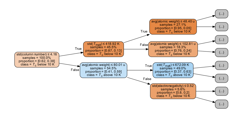
Figure 1: Schematic of the random forest ML approach. Example of a single decision tree used to classify materials depending on whether $T_{\mathrm{c}}$ is above or below $10$ K. A tree can have many levels, but only the three top are shown. The decision rules leading to each subset are written inside individual rectangles. The subset population percentage is given by “samples”, and the node color/shade represents the degree of separation, i.e., dark blue/orange illustrates a high proportion of $T_{\mathrm{c}}>10$ K/$T_{\mathrm{c}}<10$ K materials (the exact value is given by “proportion”). A random forest consists of a large number — could be hundreds or thousands — of such individual trees.

Unfortunately, only a small subset of materials in SuperCon overlaps with those in the ICSD: about $800$ with finite $T_{\mathrm{c}}$ and less than $600$ are contained within AFLOW. For these, a set of 26 predictors are incorporated from the AFLOW Online Repositories, including structural/chemical information like the lattice type, space group, volume of the unit cell, density, ratios of the lattice parameters, Bader charges and volumes, and formation energy (see Supplementary Materials). In addition, electronic properties are considered, including the density of states near the Fermi level as calculated by AFLOW. Previous investigations exposed limitations in applying ML methods to a similar dataset in isolation [25]. Instead, a framework is presented here for combining models built on Magpie descriptors (large sampling, but features limited to compositional data) and AFLOW features (small sampling, but diverse and pertinent features).

Once we have a list of relevant predictors, various ML models can be applied to the data [52, 53]. All ML algorithms in this work are variants of the random forest method [54]. Fundamentally, this approach combines many individual decision trees, where each tree is a non-parametric supervised learning method used for modeling either categorical or numerical variables (i.e., classification or regression modeling). A tree predicts the value of a target variable by learning simple decision rules inferred from the available features (see Figure 1 for an example).

Random forest is one of the most powerful, versatile, and widely-used ML methods [55]. There are several advantages that make it especially suitable for this problem. First, it can learn complicated non-linear dependencies from the data. Unlike many other methods (e.g., linear regression), it does not make any assumptions about the relationship between the predictors and the target variable. Second, random forests are quite tolerant to heterogeneity in the training data. It can handle both numerical and categorical data which, furthermore, does not need extensive and potentially dangerous preprocessing, such as scaling or normalization. Even the presence of strongly correlated predictors is not a problem for model construction (unlike many other ML algorithms). Another significant advantage of this method is that, by combining information from individual trees, it can estimate the importance of each predictor, thus making the model more interpretable. However, unlike model construction, determination of predictor importance is complicated by the presence of correlated features. To avoid this, standard feature selection procedures are employed along with a rigorous predictor elimination scheme (based on their strength and correlation with others). Overall, these methods reduce the complexity of the models and improve our ability to interpret them.

Classification models. As a first step in applying ML methods to the dataset, a sequence of classification models are created, each designed to separate materials into two distinct groups depending on whether $T_{\mathrm{c}}$ is above or below some predetermined value. The temperature that separates the two groups ($T_{\mathrm{sep}}$) is treated as an adjustable parameter of the model, though some physical considerations should guide its choice as well. Classification ultimately allows compounds with no reported $T_{\mathrm{c}}$ to be used in the training set by including them in the below-$T_{\mathrm{sep}}$ bin. Although discretizing continuous variables is not generally recommended, in this case the benefits of including compounds without $T_{\mathrm{c}}$ outweigh the potential information loss.

In order to choose the optimal value of $T_{\mathrm{sep}}$, a series of random forest models are trained with different threshold temperatures separating the two classes. Since setting $T_{\mathrm{sep}}$ too low or too high creates strongly imbalanced classes (with many more instances in one group), it is important to compare the models using several different metrics. Focusing only on the accuracy (count of correctly-classified instances) can lead to deceptive results. Hypothetically, if $95\%$ of the observations in the dataset are in the below-$T_{\mathrm{sep}}$ group, simply classifying all materials as such would yield a high accuracy ($95\%$), while being trivial in any other sense. To avoid this potential pitfall, three other standard metrics for classification are considered: precision, recall, and $F_{\mathrm{1}}$ score. They are defined using the values $tp$, $tn$, $fp$, and $fn$ for the count of true/false positive/negative predictions of the model:

$$\text{accuracy}\equiv\frac{tp+tn}{tp+tn+fp+fn},$$ (1)

$$\text{precision}\equiv\frac{tp}{tp+fp},$$ (2)

$$\text{recall}\equiv\frac{tp}{tp+fn},$$ (3)

$$F_{\mathrm{1}}\equiv 2*\frac{\text{precision}*\text{recall}}{\text{precision}+\text{recall}},$$ (4)

where positive/negative refers to above-$T_{\mathrm{sep}}$/below-$T_{\mathrm{sep}}$. The accuracy of a classifier is the total proportion of correctly-classified materials, while precision measures the proportion of correctly-classified above-$T_{\mathrm{sep}}$ superconductors out of all predicted above-$T_{\mathrm{sep}}$. The recall is the proportion of correctly-classified above-$T_{\mathrm{sep}}$ materials out of all truly above-$T_{\mathrm{sep}}$ compounds. While the precision measures the probability that a material selected by the model actually has $T_{\mathrm{c}}>T_{\mathrm{sep}}$, the recall reports how sensitive the model is to above-$T_{\mathrm{sep}}$ materials. Maximizing the precision or recall would require some compromise with the other, i.e., a model that labels all materials as above-$T_{\mathrm{sep}}$ would have perfect recall but dismal precision. To quantify the trade-off between recall and precision, their harmonic mean ($F_{\mathrm{1}}$ score) is widely used to measure the performance of a classification model. With the exception of accuracy, these metrics are not symmetric with respect to the exchange of positive and negative labels.

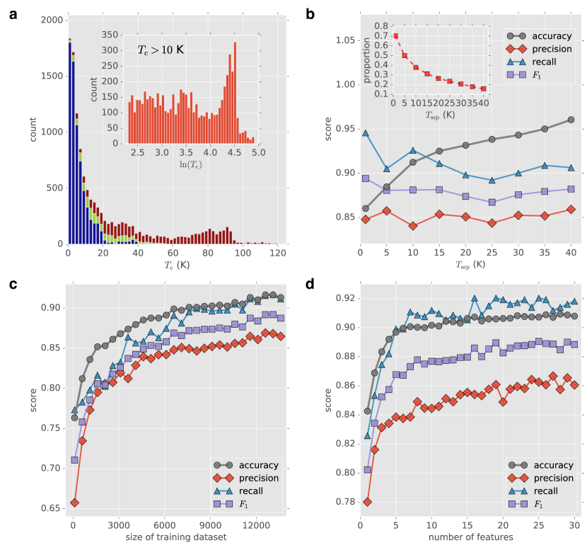
Figure 2: SuperCon dataset and classification model performance. (a) Histogram of materials categorized by $T_{\mathrm{c}}$ (bin size is $2$ K, only those with finite $T_{\mathrm{c}}$ are counted). Blue, green, and red denote “low-$T_{\mathrm{c}}$”, iron-based, and cuprate superconductors, respectively. In the inset: histogram of materials categorized by $\ln{(T_{\mathrm{c}})}$ restricted to those with $T_{\mathrm{c}}>10$ K. (b) Performance of different classification models as a function of the threshold temperature $\left(T_{\mathrm{sep}}\right)$ that separates materials in two classes by $T_{\mathrm{c}}$. Performance is measured by accuracy (gray), precision (red), recall (blue), and $F_{\mathrm{1}}$ score (purple). The scores are calculated from predictions on an independent test set, i.e., one separate from the dataset used to train the model. In the inset: the dashed red curve gives the proportion of materials in the above-$T_{\mathrm{sep}}$ set. (c) Accuracy, precision, recall, and $F_{\mathrm{1}}$ score as a function of the size of the training set with a fixed test set. (d) Accuracy, precision, recall, and $F_{\mathrm{1}}$ as a function of the number of predictors.

For a realistic estimate of the performance of each model, the dataset is randomly split ($85\%/15\%$) into training and test subsets. The training set is employed to fit the model, which is then applied to the test set for subsequent benchmarking. The aforementioned metrics (Equations 1-4) calculated on the test set provide an unbiased estimate of how well the model is expected to generalize to a new (but similar) dataset. With the random forest method, similar estimates can be obtained intrinsically at the training stage. Since each tree is trained only on a bootstrapped subset of the data, the remaining subset can be used as an internal test set. These two methods for quantifying model performance usually yield very similar results.

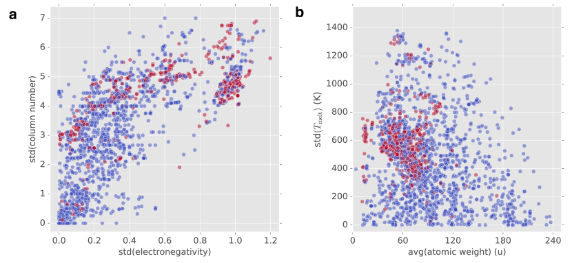
Figure 3: Scatter plots of $3,000$ superconductors in the space of the four most important classification predictors. Blue/red represent below-$T_{\mathrm{sep}}$/above-$T_{\mathrm{sep}}$ materials, where $T_{\mathrm{sep}}=10$ K. (a) Feature space of the first and second most important predictors: standard deviations of the column numbers and electronegativities (calculated over the values for the constituent elements in each compound). (b) Feature space of the third and fourth most important predictors: standard deviation of the elemental melting temperatures and average of the atomic weights.

With the procedure in place, the models’ metrics are evaluated for a range of $T_{\mathrm{sep}}$ and illustrated in Figure 2b. The accuracy increases as $T_{\mathrm{sep}}$ goes from $1$ K to $40$ K, and the proportion of above-$T_{\mathrm{sep}}$ compounds drops from above $70\%$ to about $15\%$, while the recall and $F_{\mathrm{1}}$ score generally decrease. The region between $5-15$ K is especially appealing in (nearly) maximizing all benchmarking metrics while balancing the sizes of the bins. In fact, setting $T_{\mathrm{sep}}=10$ K is a particularly convenient choice. It is also the temperature used in Refs [23, 24] to separate the two classes, as it is just above the highest $T_{\mathrm{c}}$ of all elements and pseudoelemental materials (solid solution whose range of composition includes a pure element). Here, the proportion of above-$T_{\mathrm{sep}}$ materials is approximately $38\%$ and the accuracy is about $92\%$, i.e., the model can correctly classify nine out of ten materials — much better than random guessing. The recall — quantifying how well all above-$T_{\mathrm{sep}}$ compounds are labeled and, thus, the most important metric when searching for new superconducting materials — is even higher. (Note that the models’ metrics also depend on random factors such as the composition of the training and test sets, and their exact values can vary.)

Table 1: The most relevant predictors and their importances for the classification and general regression models. $\operatorname*{avg}(x)$ and $\operatorname*{std}(x)$ denote the composition-weighted average and standard deviation, respectively, calculated over the vector of elemental values for each compound [38]. For the classification model, all predictor importances are quite close.

predictor	model
rank	classification		regression (general; $T_{\mathrm{c}}>10$ K)
1	$\operatorname*{std}($column number$)$	0.26	$\operatorname*{avg}($number of unfilled orbitals$)$	0.26
2	$\operatorname*{std}($electronegativity$)$	0.26	$\operatorname*{std}($ground state volume$)$	0.18
3	$\operatorname*{std}($melting temperature$)$	0.23	$\operatorname*{std}($space group number$)$	0.17
4	$\operatorname*{avg}($atomic weight$)$	0.24	$\operatorname*{avg}($number of $d$ unfilled orbitals$)$	0.17
5		-	$\operatorname*{std}($number of $d$ valence electrons$)$	0.12
6		-	$\operatorname*{avg}($melting temperature$)$	0.1

The most important factors that determine the model’s performance are the size of the available dataset and the number of meaningful predictors. As can be seen in Figure 2c, all metrics improve significantly with the increase of the training set size. The effect is most dramatic for sizes between several hundred and few thousands instances, but there is no obvious saturation even for the largest available datasets. This validates efforts herein to incorporate as much relevant data as possible into model training. The number of predictors is another very important model parameter. In Figure 2d, the accuracy is calculated at each step of the backward feature elimination process. It quickly saturates when the number of predictors reaches $10$. In fact, a model with only 5 predictors achieves almost $90\%$ accuracy. (Note that these are the five most informative predictors, selected by the model out of the full list of 145 ones.)

For an understanding of what the model has learned, an analysis of the chosen predictors is needed. In the random forest method, features can be ordered by their importance quantified via the so-called Gini importance or “mean decrease in impurity” [52, 53]. For a given feature, it is the sum of the Gini impurity   over the number of splits that include the feature, weighted by the number of samples it splits, and averaged over the entire forest. Due to the nature of the algorithm, the closer to the top of the tree a predictor is used, the greater number of predictions it impacts.

Although correlations between predictors do not affect the model’s ability to learn, it can distort importance estimates. For example, a material property with a strong effect on $T_{\mathrm{c}}$ can be shared among several correlated predictors. Since the model can access the same information through any of these variables, their relative importances are diluted across the group. To reduce the effect and limit the list of predictors to a manageable size, the backward feature elimination method is employed. The process begins with a model constructed with the full list of predictors, and iteratively removes the least significant one, rebuilding the model and recalculating importances with every iteration. (This iterative procedure is necessary since the ordering of the predictors by importance can change at each step.) Predictors are removed until the accuracy drops by no more than $2\%$, reducing the full list of 145 down to 5. Furthermore, two of these predictors are strongly correlated with each other, and we remove the less important one. This has a negligible impact on the model performance, yielding four predictors total (see Table 1) with an above $90\%$ accuracy score — only slightly worse than the full model. Scatter plots of the pairs of the most important predictors are shown in Figure 3, where blue/red denotes whether the material is in the below-$T_{\mathrm{sep}}$/above-$T_{\mathrm{sep}}$ class. Figure 3a shows a scatter plot of $3,000$ compounds in the space spanned by the standard deviations of the column numbers and electronegativities calculated over the elemental values. Superconductors with $T_{\mathrm{c}}>10$ K tend to cluster in the upper-right corner of the plot and in a relatively thin elongated region extending to the left of it. In fact, the points in the upper-right corner represent mostly cuprate materials, which with their complicated compositions and large number of elements are likely to have high standard deviations in these variables. Figure 3b shows the same compounds projected in the space of the standard deviations of the melting temperatures and the averages of the atomic weights of the elements forming each compound. The above-$T_{\mathrm{sep}}$ materials tend to cluster in areas with lower mean atomic weights — not a surprising result given the role of phonons in conventional superconductivity.

For comparison, we create another classifier based on the average number of valence electrons, metallic electronegativity differences, and orbital radii differences, i.e., the predictors used in Refs. [23, 24] to cluster materials with $T_{\mathrm{c}}>10$ K. A classifier built only with these three predictors is less accurate than both the full and the truncated models presented herein, but comes quite close: the full model has about $3\%$ higher accuracy and $F_{\mathrm{1}}$ score, while the truncated model with four predictors is less that $2\%$ more accurate. The rather small (albeit not insignificant) differences demonstrates that even on the scale of the entire SuperCon dataset, the predictors used by Villars and Rabe [23, 24] capture much of the relevant chemical information for superconductivity.

Regression models. After constructing a successful classification model, we now move to the more difficult challenge of predicting $T_{\mathrm{c}}$. Creating a regression model may enable better understanding of the factors controlling $T_{\mathrm{c}}$ of known superconductors, while also serving as an organic part of a system for identifying potential new ones. Leveraging the same set of elemental predictors as the classification model, several regression models are presented focusing on materials with $T_{\mathrm{c}}>10$ K. It avoids the problem of materials with no reported $T_{\mathrm{c}}$ with the assumption that, if they were to exhibit superconductivity at all, their critical temperature would be below $10$ K. Another problem is that the $T_{\mathrm{c}}$’s are unevenly distributed over the $T_{\mathrm{c}}$ axis (see Figure 2a). To avoid this, $\ln{(T_{\mathrm{c}})}$ is used as the target variable instead of $T_{\mathrm{c}}$ (Figure 2a inset), which creates a more uniform distribution and is also considered a best practice when the range of a target variable covers more than one order of magnitude (as in the case of $T_{\mathrm{c}}$). Following this transformation, the dataset is parsed randomly ($85\%$/$15\%$) into training and test subsets (similarly performed for the classification model).

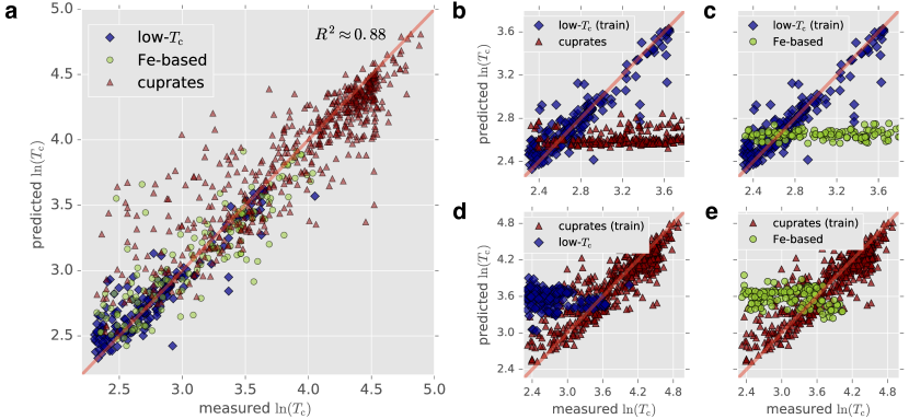
Figure 4: Benchmarking of regression models predicting $\ln(T_{\mathrm{c}})$. (a) Predicted vs. measured $\ln(T_{\mathrm{c}})$ for the general regression model. The test set comprises of a mix of low-$T_{\mathrm{c}}$, iron-based, and cuprate superconductors with $T_{\mathrm{c}}>10$ K. With an $R^{2}$ of about $0.88$, this one model can accurately predict $T_{\mathrm{c}}$ for materials in different superconducting groups. (b and c) Predictions of the regression model trained solely on low-$T_{\mathrm{c}}$ compounds for test sets containing cuprate and iron-based materials. (d and e) Predictions of the regression model trained solely on cuprates for test sets containing low-$T_{\mathrm{c}}$ and iron-based superconductors. Models trained on a single group have no predictive power for materials from other groups.

Present within the dataset are distinct families of superconductors with different driving mechanisms for superconductivity, including cuprate and iron-based high-temperature superconductors, with all others denoted “low-$T_{\mathrm{c}}$” for brevity (no specific mechanism in this group). Surprisingly, a single regression model does reasonably well among the different families – benchmarked on the test set, the model achieves $R^{2}\approx 0.88$ (Figure 4a). It suggests that the random forest algorithm is flexible and powerful enough to automatically separate the compounds into groups and create group-specific branches with distinct predictors (no explicit group labels were used during training and testing). As validation, three separate models are constructed trained only on a specific family, namely the low-$T_{\mathrm{c}}$, cuprate, and iron-based superconductors, respectively. Benchmarking on mixed-family test sets, the models performed well on compounds belonging to their training set family while demonstrating no predictive power on the others. Figures 4b-d illustrate a cross-section of this comparison. Specifically, the model trained on low-$T_{\mathrm{c}}$ compounds dramatically underestimates the $T_{\mathrm{c}}$ of both high-temperature superconducting families (Figures 4b and c), even though this test set only contains compounds with $T_{\mathrm{c}}<40$ K. Conversely, the model trained on the cuprates tends to overestimate the $T_{\mathrm{c}}$ of low-$T_{\mathrm{c}}$ (Figure 4d) and iron-based (Figure 4e) superconductors. This is a clear indication that superconductors from these groups have different factors determining their $T_{\mathrm{c}}$. Interestingly, the family-specific models do not perform better than the general regression containing all the data points: $R^{2}$ for the low-$T_{\mathrm{c}}$ materials is about $0.85$, for cuprates is just below $0.8$, and for iron-based compounds is about $0.74$. In fact, it is a purely geometric effect that the combined model has the highest $R^{2}$. Each group of superconductors contributes mostly to a distinct $T_{\mathrm{c}}$ range, and, as a result, the combined regression is better determined over longer temperature interval.

Table 2: The most significant predictors and their importances for the three material-specific regression models. $\operatorname*{avg}(x)$, $\operatorname*{std}(x)$, $\max(x)$ and $\operatorname*{frac}(x)$ denote the composition-weighted average, standard deviation, maximum, and fraction, respectively, taken over the elemental values for each compound. $l^{2}$-norm of a composition is calculated by $||x||_{2}=\sqrt{\sum_{i}x_{i}^{2}}$, where $x_{i}$ is the proportion of each element $i$ in the compound.

pred.	model
rank	regression (low-$T_{\mathrm{c}}$)		regression (cuprates)		regression (Fe-based)
1	$\operatorname*{frac}(d$ valence electrons$)$	0.18	$\operatorname*{avg}($number of unfilled orbitals$)$	0.22	$\operatorname*{std}($column number$)$	0.17
2	$\operatorname*{avg}($number of $d$ unfilled orbitals$)$	0.14	$\operatorname*{std}($number of $d$ valence electrons$)$	0.13	$\operatorname*{avg}($ionic character$)$	0.15
3	$\operatorname*{avg}($number of valence electrons$)$	0.13	$\operatorname*{frac}(d$ valence electrons$)$	0.13	$\operatorname*{std}($Mendeleev number$)$	0.14
4	$\operatorname*{frac}(s$ valence electrons$)$	0.11	$\operatorname*{std}($ground state volume$)$	0.13	$\operatorname*{std}($covalent radius$)$	0.14
5	$\operatorname*{avg}($number of $d$ valence electrons$)$	0.09	$\operatorname*{std}($number of valence electrons$)$	0.1	$\max($melting temperature$)$	0.14
6	$\operatorname*{avg}($covalent radius$)$	0.09	$\operatorname*{std}($row number$)$	0.08	$\operatorname*{avg}($Mendeleev number$)$	0.14
7	$\operatorname*{avg}($atomic weight$)$	0.08	$||$composition$||_{2}$	0.07	$||$composition$||_{2}$	0.11
8	$\operatorname*{avg}($Mendeleev number$)$	0.07	$\operatorname*{std}($number of $s$ valence electrons$)$	0.07		-
9	$\operatorname*{avg}($space group number$)$	0.07	$\operatorname*{std}($melting temperature$)$	0.07		-
10	$\operatorname*{avg}($number of unfilled orbitals$)$	0.06		-		-

In order to reduce the number of predictors and increase the interpretability of these models without significant detriment to their performance, a backward feature elimination process is again employed. The procedure is very similar to the one described previously for the classification model, with the only difference being that the reduction is guided by $R^{2}$ of the model, rather than the accuracy (the procedure stops when $R^{2}$ drops by $3\%$).

The most important predictors for the four models (one general and three family-specific) together with their importances are shown in Tables 1 and 2. Differences in important predictors across the family-specific models reflect the fact that distinct mechanisms are responsible for driving superconductivity among these groups. The list is longest for the low-$T_{\mathrm{c}}$ superconductors, reflecting the eclectic nature of this group. Similar to the general regression model, different branches are likely created for distinct sub-groups. Nevertheless, some important predictors have straightforward interpretation. As illustrated in Figure 5a, low average atomic weight is a necessary (albeit not sufficient) condition for achieving high $T_{\mathrm{c}}$ among the low-$T_{\mathrm{c}}$ group. In fact, the maximum $T_{\mathrm{c}}$ for a given weight roughly follows $1/\sqrt{m_{A}}$. Mass plays a significant role in conventional superconductors through the Debye frequency of phonons, leading to the well-known formula $T_{\mathrm{c}}\sim 1/\sqrt{m}$, where $m$ is the ionic mass. Other factors like density of states are also important, which explains the spread in $T_{\mathrm{c}}$ for a given $m_{A}$. Outlier materials clearly lying above the $\sim 1/\sqrt{m_{A}}$ line include bismuthates and chloronitrates, suggesting the conventional electron-phonon mechanism is not driving superconductivity in these materials. Indeed, chloronitrates exhibit a very weak isotope effect [57], though some unconventional electron-phonon coupling could still be relevant for superconductivity [58]. Another important feature for low-$T_{\mathrm{c}}$ materials is the average number of valence electrons. This recovers the empirical relation first discovered by Matthias more than sixty years ago [59]. Such findings validate the ability of ML approaches to discover meaningful patterns that encode true physical phenomena.

Similar $T_{\mathrm{c}}$-vs.-predictor plots reveal more interesting and subtle features. A narrow cluster of materials with $T_{\mathrm{c}}>20$ K emerges in the context of the mean covalent radii of compounds — another important predictor for low-$T_{\mathrm{c}}$ superconductors. The cluster includes (left-to-right) alkali-doped C₆₀, MgB₂-related compounds, and bismuthates. The sector likely characterizes a region of strong covalent bonding and corresponding high-frequency phonon modes that enhance $T_{\mathrm{c}}$ (however, frequencies that are too high become irrelevant for superconductivity). Another interesting relation appears in the context of the average number of $d$ valence electrons. Figure 5c illustrates a fundamental bound on $T_{\mathrm{c}}$ of all non-cuprate and non-iron-based superconductors.

A similar limit exists for cuprates based on the average number of unfilled orbitals (Figure  5d). It appears to be quite rigid — several data points found above it on inspection are actually incorrectly recorded entries in the database and were subsequently removed. The connection between $T_{\mathrm{c}}$ and the average number of unfilled orbitals  may offer new insight into the mechanism for superconductivity in this family. Known trends include higher $T_{\mathrm{c}}$’s for structures that (i) stabilize more than one superconducting Cu-O plane per unit cell and (ii) add more polarizable cations such as Tl³⁺ and Hg²⁺ between these planes. The connection reflects these observations, since more copper and oxygen per formula unit leads to lower average number of unfilled orbitals (one for copper, two for oxygen). Further, the lower-$T_{\mathrm{c}}$ cuprates typically consist of Cu^2-/Cu^3--containing layers stabilized by the addition/substition of hard cations, such as Ba²⁺ and La³⁺, respectively. These cations have a large number of unfilled orbitals, thus increasing the compound’s average. Therefore, the ability of between-sheet cations to contribute charge to the Cu-O planes may be indeed quite important. The more polarizable the $A$ cation, the more electron density it can contribute to the already strongly covalent Cu²⁺–O bond.

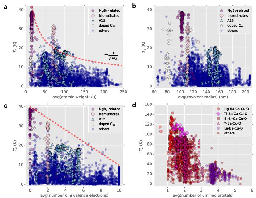
Figure 5: Scatter plots of $T_{\mathrm{c}}$ for superconducting materials in the space of significant, family-specific regression predictors. For $4,000$ “low-$T_{\mathrm{c}}$” superconductors (i.e., non-cuprate and non-iron-based), $T_{\mathrm{c}}$ is plotted vs. the (a) average atomic weight, (b) average covalent radius, and (c) average number of $d$ valence electrons. The dashed red line in (a) is $\sim 1/\sqrt{m_{A}}$. Having low average atomic weight and low average number of $d$ valence electrons are necessary (but not sufficient) conditions for achieving high $T_{\mathrm{c}}$ in this group. (d) Scatter plot of $T_{\mathrm{c}}$ for all known superconducting cuprates vs. the mean number of unfilled orbitals. (c and d) suggest that the values of these predictors lead to hard limits on the maximum achievable $T_{\mathrm{c}}$.

Including AFLOW. The models described previously demonstrate surprising accuracy and predictive power, especially considering the difference between the relevant energy scales of most Magpie predictors (typically in the range of eV) and superconductivity (meV scale). This disparity, however, hinders the interpretability of the models, i.e., the ability to extract meaningful physical correlations. Thus, it is highly desirable to create accurate ML models with features based on measurable macroscopic properties of the actual compounds (e.g., crystallographic and electronic properties) rather than composite elemental predictors. Unfortunately, only a small subset of materials in SuperCon is also included in the ICSD: about $1,500$ compounds in total, only about $800$ with finite $T_{\mathrm{c}}$, and even fewer are characterized with ab initio calculations. In fact, a good portion of known superconductors are disordered (off-stoichiometric) materials and notoriously challenging to address with DFT calculations. Currently, much faster and efficient methods are becoming available [40] for future applications.

To extract suitable features, data is incorporated from the AFLOW Online Repositories — a database of DFT calculations managed by the software package AFLOW. It contains information for the vast majority of compounds in the ICSD and about 550 superconducting materials. In Ref. 25, several ML models using a similar set of materials are presented. Though a classifier shows good accuracy, attempts to create a regression model for $T_{\mathrm{c}}$ led to disappointing results. We verify that using Magpie predictors for the superconducting compounds in the ICSD also yields an unsatisfactory regression model. The issue is not the lack of compounds per se, as models created with randomly drawn subsets from SuperCon with similar counts of compounds perform much better. In fact, the problem is the chemical sparsity of superconductors in the ICSD, i.e., the dearth of closely-related compounds (usually created by chemical substitution). This translates to compound scatter in predictor space — a challenging learning environment for the model.

Table 3: List of potential superconductors identified by the pipeline. Also shown are their ICSD numbers and symmetries. Note that for some compounds there are several entries. All of the materials contain oxygen.

compound	ICSD	SYM
CsBe(AsO4)	074027	orthorhombic
RbAsO2	413150	orthorhombic
KSbO2	411214	monoclinic
RbSbO2	411216	monoclinic
CsSbO2	059329	monoclinic
AgCrO2	004149/025624	hexagonal
K0.8(Li0.2Sn0.76)O2	262638	hexagonal
Cs(MoZn)(O3F3)	018082	cubic
Na3Cd2(IrO6)	404507	monoclinic
Sr3Cd(PtO6)	280518	hexagonal
Sr3Zn(PtO6)	280519	hexagonal
(Ba5Br${}_{2})$Ru2O9	245668	hexagonal
Ba4(AgO2)(AuO${}_{4})$	072329	orthorhombic
Sr5(AuO4)2	071965	orthorhombic
RbSeO2F	078399	cubic
CsSeO2F	078400	cubic
KTeO2F	411068	monoclinic
Na2K4(Tl2O6)	074956	monoclinic
Na3Ni2BiO6	237391	monoclinic
Na3Ca2BiO6	240975	orthorhombic
CsCd(BO3)	189199	cubic
K2Cd(SiO${}_{4})$	083229/086917	orthorhombic
Rb2Cd(SiO4)	093879	orthorhombic
K2Zn(SiO4)	083227	orthorhombic
K2Zn(Si2O6)	079705	orthorhombic
K2Zn(GeO4)	069018/085006/085007	orthorhombic
(K0.6Na${}_{1.4})$Zn(GeO${}_{4})$	069166	orthorhombic
K2Zn(Ge2O6)	065740	orthorhombic
Na6Ca3(Ge2O6)3	067315	hexagonal
Cs3(AlGe2O7)	412140	monoclinic
K4Ba(Ge3O9)	100203	monoclinic
K16Sr4(Ge3O9)4	100202	cubic
K3Tb[Ge3O8(OH)2]	193585	orthorhombic
K3Eu[Ge3O8(OH)2]	262677	orthorhombic
KBa6Zn4(Ga7O21)	040856	trigonal

The chemical sparsity in ICSD superconductors is a significant hurdle, even when both sets of predictors (i.e., Magpie and AFLOW features) are combined via feature fusion. Additionally, this approach alone neglects the majority of the $16,000$ compounds available via SuperCon. Instead, we constructed separate models employing Magpie and AFLOW features, and then judiciously combined the results to improve model metrics — known as late or decision-level fusion. Specifically, two independent classification models are developed, one using the full SuperCon dataset and Magpie predictors, and another based on superconductors in the ICSD and AFLOW predictors. Such an approach can improve the recall, for example, in the case where we classify “high-$T_{\mathrm{c}}$” superconductors as those predicted by either model to be above-$T_{\mathrm{sep}}$. Indeed, this is the case here where, separately, the models obtain a recall of $40\%$ and $66\%$, respectively, and together achieve a recall of about $76\%$ (subject to small fluctuations due to variations in the test sets). In this way, the models’ predictions complement each other in a constructive way such that above-$T_{\mathrm{sep}}$ materials missed by one model (but not the other) are now accurately classified.

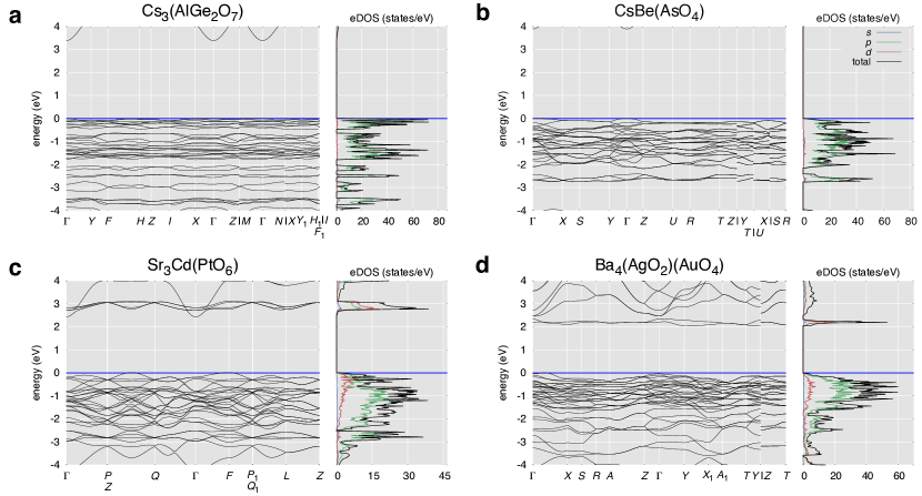
Figure 6: DOS of four compounds identified by the ML algorithm as potential materials with $T_{\mathrm{c}}>20$ K. The partial DOS contributions from $s$, $p$ and $d$ electrons and total DOS are shown in blue, green, red, and black, respectively. The large peak just below $E_{F}$ is a direct consequence of the flat band(s) present in all these materials. These images were generated automatically via AFLOW [43]. In the case of substantial overlap among k-point labels, the right-most label is offset below.

Searching for new superconductors in the ICSD. As a final proof of concept demonstration, the classification and regression models described previously are integrated in one pipeline and employed to screen the entire ICSD database for candidate “high-$T_{\mathrm{c}}$” superconductors. (Note that “high-$T_{\mathrm{c}}$” is a simple label, the precise meaning of which can be adjusted.) Similar tools power high-throughput screening workflows for materials with desired thermal conductivity and magnetocaloric properties [51, 61]. As a first step, the full set of Magpie predictors are generated for all compounds in SuperCon. A classification model similar to the one presented above is constructed, but trained only on materials in SuperCon and not in the ICSD (used as an independent test set). The model is then applied on the ICSD set to create a list of materials with predicted $T_{\mathrm{c}}$ above $10$ K. Opportunities for model benchmarking are limited to those materials both in the SuperCon and ICSD datasets, though this test set is shown to be problematic. The set includes about $1,500$ compounds, though $T_{\mathrm{c}}$ is reported for only about half of them. The model achieves an impressive accuracy of $0.98$, which is overshadowed by the fact that $96.6\%$ of these compounds belong to the $T_{\mathrm{c}}<10$ K class. The precision, recall, and $F_{\mathrm{1}}$ scores are about $0.74$, $0.66$, and $0.70$, respectively. These metrics are lower than the estimates calculated for the general classification model, which is not unexpected given that this set cannot be considered randomly selected. Nevertheless, the performance suggests a good opportunity to identify new candidate superconductors.

Next in the pipeline, the list is fed into a random forest regression model (trained on the entire SuperCon database) to predict $T_{\mathrm{c}}$. Filtering on the materials with $T_{\mathrm{c}}>20$ K, the list is further reduced to about $2,000$ compounds. This count may appear daunting, but should be compared with the total number of compounds in the database — about $110,000$. Thus, the method selects less than two percent of all materials, which in the context of the training set (containing more than $20\%$ with “high-$T_{\mathrm{c}}$”), suggests that the model is not overly biased toward predicting high critical temperatures.

The vast majority of the compounds identified as candidate superconductors are cuprates, or at least compounds that contain copper and oxygen. There are also some materials clearly related to the iron-based superconductors. The remaining set has 35 members, and is composed of materials that are not obviously connected to any high-temperature superconducting families (see Table 3) [62]. None of them is predicted to have $T_{\mathrm{c}}$ in excess of $40$ K, which is not surprising, given that no such instances exist in the training dataset. All contain oxygen — also not a surprising result, since the group of known superconductors with $T_{\mathrm{c}}>20$ K is dominated by oxides.

The list comprises several distinct groups. Especially interesting are the compounds containing heavy metals (such as Au, Ir, Ru), metalloids (Se, Te), and heavier post-transition metals (Bi, Tl), which are or could be pushed into interesting/unstable oxidation states. Charge doping and/or pressure may be needed to drive these materials into a superconducting state. The most surprising and non-intuitive of the compounds in the list are the silicates and the germanates. These materials form corner-sharing SiO₄ or GeO₄ polyhedra, not unlike quartz glass, and also have counter cations with full or empty shells such as Cd₂⁺ or K⁺. Converting these insulators to metals (and possibly superconductors) likely requires significant charge doping. However, the similarity between these compounds and cuprates is meaningful. In compounds like K₂CdSiO₄ or K₂ZnSiO₄, K₂Cd (or K₂Zn) unit carries a 4+ charge that offsets the (SiO₄)^4- (or (GeO₄)^4-) charges. This is reminiscent of the way Sr₂ balances the (CuO₄)^4- unit in Sr₂CuO₄. Such chemical similarities based on charge balancing and stoichiometry were likely identified and exploited by the ML algorithms.

The electronic properties calculated by AFLOW offer additional insight into the results of the search, and suggest a possible connection among these candidate. Plotting the electronic structure of the potential superconductors exposes an extremely peculiar feature shared by almost all — one or several (nearly) flat bands just below the energy of the highest occupied electronic state. Such bands lead to a large peak in the DOS (see Figure 6) and can cause a significant enhancement in $T_{\mathrm{c}}$. Peaks in the DOS elicited by van Hove singularities can enhance $T_{\mathrm{c}}$ if sufficiently close to $E_{\mathrm{F}}$ [63, 64, 65]. However, note that unlike typical van Hove points, a true flat band creates divergence in the DOS (as opposed to its derivatives), which in turn leads to a critical temperature dependence linear in the pairing interaction strength, rather than the usual exponential relationship yielding lower $T_{\mathrm{c}}$ [33]. Additionally, there is significant similarity with the band structure and DOS of layered BiS₂-based superconductors [66].

This band structure feature came as the surprising result of applying the ML model. It was not sought for, and, moreover, no explicit information about the electronic band structure has been included in these predictors. This is in contrast to the algorithm presented in Ref. 30, which was specifically designed to filter ICSD compounds based on several preselected electronic structure features.

While at the moment it is not clear if some (or indeed any) of these compounds are really superconducting, let alone with $T_{\mathrm{c}}$’s above 20 K, the presence of this highly unusual electronic structure feature is encouraging. Attempts to synthesize several of these compounds are already underway.

Discussion

Herein, several machine learning tools are developed to study the critical temperature of superconductors. Based on information from the SuperCon database, initial coarse-grained chemical features are generated using the Magpie software. As a first application of ML methods, materials are divided into two classes depending on whether $T_{\mathrm{c}}$ is above or below $10$ K. A non-parametric random forest classification model is constructed to predict the class of superconductors. The classifier shows excellent performance, with out-of-sample accuracy and $F_{\mathrm{1}}$ score of about $92\%$. Next, several successful random forest regression models are created to predict the value of $T_{\mathrm{c}}$, including separate models for three material sub-groups, i.e., cuprate, iron-based, and “low-$T_{\mathrm{c}}$” compounds. By studying the importance of predictors for each family of superconductors, insights are obtained about the physical mechanisms driving superconductivity among the different groups. With the incorporation of crystallographic-/electronic-based features from the AFLOW Online Repositories, the ML models are further improved. Finally, we combined these models into one integrated pipeline, which is employed to search the entire ICSD database for new inorganic superconductors. The model identified about 30 oxides as candidate materials. Some of these are chemically and structurally similar to cuprates (even though no explicit structural information was provided during training of the model). Another feature that unites almost all of these materials is the presence of flat or nearly-flat bands just below the energy of the highest occupied electronic state.

In conclusion, this work demonstrates the important role ML models can play in superconductivity research. Records collected over several decades in SuperCon and other relevant databases can be consumed by ML models, generating insights and promoting better understanding of the connection between materials’ chemistry/structure and superconductivity. Application of sophisticated ML algorithms has the potential to dramatically accelerate the search for candidate high-temperature superconductors.

Methods

Superconductivity data. The SuperCon database consists of two separate subsets: “Oxide & Metallic” (inorganic materials containing metals, alloys, cuprate high-temperature superconductors, etc.) and “Organic” (organic superconductors). Downloading the entire inorganic materials dataset and removing compounds with incompletely-specified chemical compositions leaves about $22,000$ entries. In the case of multiple records for the same material, the reported material’s $T_{\mathrm{c}}$’s are averaged, but only if their standard deviation is less than $5$ K, and discarded otherwise. This brings the total down to about $16,400$ compounds, of which around $4,000$ have no critical temperature reported. Each entry in the set contains fields for the chemical composition, $T_{\mathrm{c}}$, structure, and a journal reference to the information source. Here, structural information is ignored as it is not always available.

There are occasional problems with the validity and consistency of some of the data. For example, the database includes some reports based on tenuous experimental evidence and only indirect signatures of superconductivity, as well as reports of inhomogeneous (surface, interfacial) and nonequilibrium phases. Even in cases of bona fide bulk superconducting phases, important relevant variables like pressure are not recorded. Though some of the obviously erroneous records were removed from the data, these issues were largely ignored assuming their effect on the entire dataset to be relatively modest. The data cleaning and processing is carried out using the Python Pandas package for data analysis [67].

Chemical and structural features. The predictors are calculated using the Magpie software [68]. It computes a set of 145 attributes for each material, including: (i) stoichiometric features (depends only on the ratio of elements and not the specific species); (ii) elemental property statistics: the mean, mean absolute deviation, range, minimum, maximum, and mode of 22 different elemental properties (e.g., period/group on the periodic table, atomic number, atomic radii, melting temperature); (iii) electronic structure attributes: the average fraction of electrons from the $s$, $p$, $d$ and $f$ valence shells among all elements present; and (iv) ionic compound features that include whether it is possible to form an ionic compound assuming all elements exhibit a single oxidation state.

ML models are also constructed with the superconducting materials in the AFLOW Online Repositories. AFLOW is a high-throughput ab initio framework that manages density functional theory (DFT) calculations in accordance with the AFLOW Standard [21]. The Standard ensures that the calculations and derived properties are empirical (reproducible), reasonably well-converged, and above all, consistent (fixed set of parameters), a particularly attractive feature for ML modeling. Many materials properties important for superconductivity have been calculated within the AFLOW framework, and are easily accessible through the AFLOW Online Repositories. The features are built with the following properties: number of atoms, space group, density, volume, energy per atom, electronic entropy per atom, valence of the cell, scintillation attenuation length, the ratios of the unit cell’s dimensions, and Bader charges and volumes. For the Bader charges and volumes (vectors), the following statistics are calculated and incorporated: the maximum, minimum, average, standard deviation, and range.

Machine learning algorithms. Once we have a list of relevant predictors, various ML models can be applied to the data [52, 53]. All ML algorithms in this work are variants of the random forest method [54]. It is based on creating a set of individual decision trees (hence the “forest”), each built to solve the same classification/regression problem. The model then combines their results, either by voting or averaging depending on the problem. The deeper individual tree are, the more complex the relationships the model can learn, but also the greater the danger of overfitting, i.e., learning some irrelevant information or just “noise”. To make the forest more robust to overfitting, individual trees in the ensemble are built from samples drawn with replacement (a bootstrap sample) from the training set. In addition, when splitting a node during the construction of a tree, the model chooses the best split of the data only considering a random subset of the features.

The random forest models above are developed using scikit-learn — a powerful and efficient machine learning Python library [69]. Hyperparameters of these models include the number of trees in the forest, the maximum depth of each tree, the minimum number of samples required to split an internal node, and the number of features to consider when looking for the best split. To optimize the classifier and the combined/family-specific regressors, the GridSearch function in scikit-learn is employed, which generates and compares candidate models from a grid of parameter values. To reduce computational expense, models are not optimized at each step of the backward feature selection process.

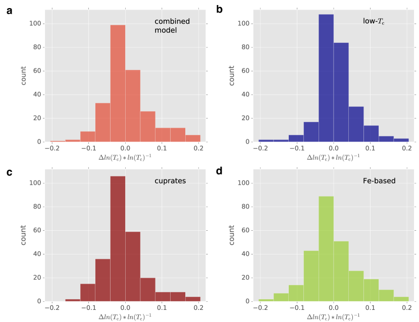
Figure 7: Histograms of $\Delta\ln(T_{\mathrm{c}})*\ln(T_{\mathrm{c}})^{-1}$ for the four regression models. $\Delta\ln(T_{\mathrm{c}})\equiv(\ln(T^{\mathrm{meas}}_{\mathrm{c}})-\ln(T^{\mathrm{pred}}_{\mathrm{c}}))$ and $\ln(T_{\mathrm{c}})\equiv\ln(T^{\mathrm{meas}}_{\mathrm{c}})$.

Prediction errors of the regression models. Previously, several regression models were described, each one designed to predict the critical temperatures of materials from different superconducting groups. These models achieved an impressive $R^{2}$ score, demonstrating good predictive power for each group. However, it is also important to consider the accuracy of the predictions for individual compounds (rather than on the aggregate set), especially in the context of searching for new materials. To do this, we calculate the prediction errors for about 300 materials from a test set. Specifically, we consider the difference between the logarithm of the predicted and measured critical temperature $[\ln(T^{\mathrm{meas}}_{\mathrm{c}})-\ln(T^{\mathrm{pred}}_{\mathrm{c}})]$ normalized by the value of $\ln(T^{\mathrm{meas}}_{\mathrm{c}})$ (normalization compensates the different $T_{\mathrm{c}}$ ranges of different groups). The models show comparable spread of errors. The histograms of errors for the four models (combined and three group-specific) are shown in Fig. 7. The errors approximately follow a normal distribution, centered not at zero but at a small negative value. This suggests the models are marginally biased, and on average tend to slightly underestimate $T_{\mathrm{c}}$. The variance is comparable for all models, but largest for the model trained and tested on iron-based materials, which also shows the smallest $R^{2}$. Performance of this model is expected to benefit from a larger training set.

References

- [1] J. E. Hirsch, M. B. Maple, and F. Marsiglio, Superconducting Materials: Conventional, Unconventional and Undetermined, Physica C 514, 1–444 (2015).
- [2] P. W. Anderson, Plasmons, Gauge Invariance, and Mass, Phys. Rev. 130, 439–442 (1963).
- [3] C. W. Chu, L. Z. Deng, and B. Lv, Hole-doped cuprate high temperature superconductors, Physica C 514, 290–313 (2015). Superconducting Materials: Conventional, Unconventional and Undetermined.
- [4] J. Paglione and R. L. Greene, High-temperature superconductivity in iron-based materials, Nature Physics 6, 645–-658 (2010).
- [5] G. Bergerhoff, R. Hundt, R. Sievers, and I. D. Brown, The inorganic crystal structure data base, J. Chem. Inf. Comput. Sci. 23, 66–69 (1983).
- [6] S. Curtarolo, W. Setyawan, G. L. W. Hart, M. Jahnátek, R. V. Chepulskii, R. H. Taylor, S. Wang, J. Xue, K. Yang, O. Levy, M. J. Mehl, H. T. Stokes, D. O. Demchenko, and D. Morgan, AFLOW: An automatic framework for high-throughput materials discovery, Comput. Mater. Sci. 58, 218–226 (2012).
- [7] D. D. Landis, J. Hummelshøj, S. Nestorov, J. Greeley, M. Dułak, T. Bligaard, J. K. Nørskov, and K. W. Jacobsen, The Computational Materials Repository, Comput. Sci. Eng. 14, 51–57 (2012).
- [8] J. E. Saal, S. Kirklin, M. Aykol, B. Meredig, and C. Wolverton, Materials Design and Discovery with High-Throughput Density Functional Theory: The Open Quantum Materials Database (OQMD), JOM 65, 1501–1509 (2013).
- [9] A. Jain, S. P. Ong, G. Hautier, W. Chen, W. D. Richards, S. Dacek, S. Cholia, D. Gunter, D. Skinner, G. Ceder, and K. A. Persson, Commentary: The Materials Project: A materials genome approach to accelerating materials innovation, APL Mater. 1, 011002 (2013).
- [10] A. Agrawal and A. Choudhary, Perspective: Materials informatics and big data: Realization of the “fourth paradigm” of science in materials science, APL Mater. 4, 053208 (2016).
- [11] T. Lookman, F. J. Alexander, and K. Rajan, eds., A Perspective on Materials Informatics: State-of-the-Art and Challenges (Springer International Publishing, 2016), doi:10.1007/978-3-319-23871-5.
- [12] A. Jain, G. Hautier, S. P. Ong, and K. A. Persson, New opportunities for materials informatics: Resources and data mining techniques for uncovering hidden relationships, J. Mater. Res. 31, 977–994 (2016).
- [13] T. Mueller, A. G. Kusne, and R. Ramprasad, Machine Learning in Materials Science (John Wiley & Sons, Inc, 2016), pp. 186–273, doi:10.1002/9781119148739.ch4.
- [14] A. Seko, T. Maekawa, K. Tsuda, and I. Tanaka, Machine learning with systematic density-functional theory calculations: Application to melting temperatures of single- and binary-component solids, Phys. Rev. B 89 (2014).
- [15] P. V. Balachandran, J. Theiler, J. M. Rondinelli, and T. Lookman, Materials Prediction via Classification Learning, Sci. Rep. 5 (2015).
- [16] G. Pilania, A. Mannodi-Kanakkithodi, B. P. Uberuaga, R. Ramprasad, J. E. Gubernatis, and T. Lookman, Machine learning bandgaps of double perovskites, Sci. Rep. 6, 19375 (2016).
- [17] O. Isayev, C. Oses, C. Toher, E. Gossett, S. Curtarolo, and A. Tropsha, Universal fragment descriptors for predicting electronic properties of inorganic crystals, Nat. Commun. 8, 15679 (2017).
- [18] National Institute of Materials Science, Materials Information Station, SuperCon, http://supercon.nims.go.jp/index_en.html (2011).
- [19] S. Curtarolo, W. Setyawan, S. Wang, J. Xue, K. Yang, R. H. Taylor, L. J. Nelson, G. L. W. Hart, S. Sanvito, M. Buongiorno Nardelli, N. Mingo, and O. Levy, AFLOWLIB.ORG: A distributed materials properties repository from high-throughput ab initio calculations, Comput. Mater. Sci. 58, 227–235 (2012).
- [20] R. H. Taylor, F. Rose, C. Toher, O. Levy, K. Yang, M. Buongiorno Nardelli, and S. Curtarolo, A RESTful API for exchanging materials data in the AFLOWLIB.org consortium, Comput. Mater. Sci. 93, 178–192 (2014).
- [21] C. E. Calderon, J. J. Plata, C. Toher, C. Oses, O. Levy, M. Fornari, A. Natan, M. J. Mehl, G. L. W. Hart, M. Buongiorno Nardelli, and S. Curtarolo, The AFLOW standard for high-throughput materials science calculations, Comput. Mater. Sci. 108 Part A, 233–238 (2015).
- [22] F. Rose, C. Toher, E. Gossett, C. Oses, M. Buongiorno Nardelli, M. Fornari, and S. Curtarolo, AFLUX: The LUX materials search API for the AFLOW data repositories, Comput. Mater. Sci. 137, 362–370 (2017).
- [23] P. Villars and J. C. Phillips, Quantum structural diagrams and high- superconductivity, Phys. Rev. B 37, 2345–2348 (1988).
- [24] K. M. Rabe, J. C. Phillips, P. Villars, and I. D. Brown, Global multinary structural chemistry of stable quasicrystals, high- ferroelectrics, and high- superconductors, Phys. Rev. B 45, 7650–7676 (1992).
- [25] O. Isayev, D. Fourches, E. N. Muratov, C. Oses, K. Rasch, A. Tropsha, and S. Curtarolo, Materials Cartography: Representing and Mining Materials Space Using Structural and Electronic Fingerprints, Chem. Mater. 27, 735–743 (2015).
- [26] J. Ling, M. Hutchinson, E. Antono, S. Paradiso, and B. Meredig, High-Dimensional Materials and Process Optimization Using Data-Driven Experimental Design with Well-Calibrated Uncertainty Estimates, Integr. Mater. Manuf. Innov. (2017).
- [27] J. E. Hirsch, Correlations between normal-state properties and superconductivity, Phys. Rev. B 55, 9007–9024 (1997).
- [28] T. O. Owolabi, K. O. Akande, and S. O. Olatunji, Estimation of Superconducting Transition Temperature for Superconductors of the Doped MgB2 System from the Crystal Lattice Parameters Using Support Vector Regression, J. Supercond. Nov. Magn. 28, 75–81 (2015).
- [29] M. Ziatdinov, A. Maksov, L. Li, A. S. Sefat, P. Maksymovych, and S. V. Kalinin, Deep data mining in a real space: separation of intertwined electronic responses in a lightly doped BaFe2As2, Nanotechnology 27, 475706 (2016).
- [30] M. Klintenberg and O. Eriksson, Possible high-temperature superconductors predicted from electronic structure and data-filtering algorithms, Comput. Mater. Sci. 67, 282–286 (2013).
- [31] T. O. Owolabi, K. O. Akande, and S. O. Olatunji, Prediction of superconducting transition temperatures for Fe-based superconductors using support vector machine. Adv. Phys. Theor. Appl. 35, 12-–26 (2014).
- [32] M. R. Norman, Materials design for new superconductors, Rep. Prog. Phys. 79, 074502 (2016).
- [33] N. B. Kopnin, T. T. Heikkilä, and G. E. Volovik, High-temperature surface superconductivity in topological flat-band systems, Phys. Rev. B 83, 220503 (2011).
- [34] S. Peotta and P. Törmä, Superfluidity in topologically nontrivial flat bands, Nat. Commun. 6, 8944 (2015).
- [35] N.B., a model suffering from selection bias can still provide valuable statistical information about known superconductors.
- [36] H. Hosono, K. Tanabe, E. Takayama-Muromachi, H. Kageyama, S. Yamanaka, H. Kumakura, M. Nohara, H. Hiramatsu, and S. Fujitsu, Exploration of new superconductors and functional materials, and fabrication of superconducting tapes and wires of iron pnictides, Sci. Technol. Adv. Mater. 16, 033503 (2015).
- [37] There are theoretical arguments for this — according to the Kohn-Luttinger theorem, a superconducting instability should be present as in any fermionic metallic system with Coulomb interactions (W. Kohn and J. M. Luttinger, New Mechanism for Superconductivity, Phys. Rev. Lett. 15, 524–526 (1965)).
- [38] L. Ward, A. Agrawal, A. Choudhary, and C. Wolverton, A general-purpose machine learning framework for predicting properties of inorganic materials, npg Computational Materials 2, 16028 (2016).
- [39] W. Setyawan and S. Curtarolo, High-throughput electronic band structure calculations: Challenges and tools, Comput. Mater. Sci. 49, 299–312 (2010).
- [40] K. Yang, C. Oses, and S. Curtarolo, Modeling Off-Stoichiometry Materials with a High-Throughput Ab-Initio Approach, Chem. Mater. 28, 6484–6492 (2016).
- [41] O. Levy, M. Jahnátek, R. V. Chepulskii, G. L. W. Hart, and S. Curtarolo, Ordered Structures in Rhenium Binary Alloys from First-Principles Calculations, J. Am. Chem. Soc. 133, 158–163 (2011).
- [42] O. Levy, G. L. W. Hart, and S. Curtarolo, Structure maps for hcp metals from first-principles calculations, Phys. Rev. B 81, 174106 (2010).
- [43] O. Levy, R. V. Chepulskii, G. L. W. Hart, and S. Curtarolo, The New face of Rhodium Alloys: Revealing Ordered Structures from First Principles, J. Am. Chem. Soc. 132, 833–837 (2010).
- [44] O. Levy, G. L. W. Hart, and S. Curtarolo, Uncovering Compounds by Synergy of Cluster Expansion and High-Throughput Methods, J. Am. Chem. Soc. 132, 4830–4833 (2010).
- [45] G. L. W. Hart, S. Curtarolo, T. B. Massalski, and O. Levy, Comprehensive Search for New Phases and Compounds in Binary Alloy Systems Based on Platinum-Group Metals, Using a Computational First-Principles Approach, Phys. Rev. X 3, 041035 (2013).
- [46] M. J. Mehl, D. Hicks, C. Toher, O. Levy, R. M. Hanson, G. L. W. Hart, and S. Curtarolo, The AFLOW Library of Crystallographic Prototypes: Part 1, Comput. Mater. Sci. 136, S1–S828 (2017).
- [47] A. R. Supka, T. E. Lyons, L. S. I. Liyanage, P. D’Amico, R. Al Rahal Al Orabi, S. Mahatara, P. Gopal, C. Toher, D. Ceresoli, A. Calzolari, S. Curtarolo, M. Buongiorno Nardelli, and M. Fornari, AFLOW: A minimalist approach to high-throughput ab initio calculations including the generation of tight-binding hamiltonians, Comput. Mater. Sci. 136, 76–84 (2017).
- [48] C. Toher, J. J. Plata, O. Levy, M. de Jong, M. D. Asta, M. Buongiorno Nardelli, and S. Curtarolo, High-throughput computational screening of thermal conductivity, Debye temperature, and Grüneisen parameter using a quasiharmonic Debye model, Phys. Rev. B 90, 174107 (2014).
- [49] E. Perim, D. Lee, Y. Liu, C. Toher, P. Gong, Y. Li, W. N. Simmons, O. Levy, J. J. Vlassak, J. Schroers, and S. Curtarolo, Spectral descriptors for bulk metallic glasses based on the thermodynamics of competing crystalline phases, Nat. Commun. 7, 12315 (2016).
- [50] C. Toher, C. Oses, J. J. Plata, D. Hicks, F. Rose, O. Levy, M. de Jong, M. D. Asta, M. Fornari, M. Buongiorno Nardelli, and S. Curtarolo, Combining the AFLOW GIBBS and Elastic Libraries to efficiently and robustly screen thermomechanical properties of solids, Phys. Rev. Materials 1, 015401 (2017).
- [51] A. van Roekeghem, J. Carrete, C. Oses, S. Curtarolo, and N. Mingo, High-Throughput Computation of Thermal Conductivity of High-Temperature Solid Phases: The Case of Oxide and Fluoride Perovskites, Phys. Rev. X 6, 041061 (2016).
- [52] C. Bishop, Pattern Recognition and Machine Learning (Springer-Verlag, New York, 2006).
- [53] T. Hastie, R. Tibshirani, and J. H. Friedman, The Elements of Statistical Learning: Data Mining, Inference, and Prediction (Springer-Verlag, New York, 2001).
- [54] L. Breiman, Random Forests, Mach. Learn. 45, 5–32 (2001).
- [55] R. Caruana and A. Niculescu-Mizil, An Empirical Comparison of Supervised Learning Algorithms, in Proceedings of the 23rd International Conference on Machine Learning, ICML ’06 (ACM, New York, NY, USA, 2006), pp. 161–168, doi:10.1145/1143844.1143865.
- [56] Gini impurity is calculated as , where is the probability of randomly chosen data point from a given decision tree leaf to be in class [52, 53].
- [57] Y. Kasahara, K. Kuroki, S. Yamanaka, and Y. Taguchi, Unconventional superconductivity in electron-doped layered metal nitride halides N ( = Ti, Zr, Hf; = Cl, Br, I), Physica C 514, 354–367 (2015). Superconducting Materials: Conventional, Unconventional and Undetermined.
- [58] Z. P. Yin, A. Kutepov, and G. Kotliar, Correlation-Enhanced Electron-Phonon Coupling: Applications of and Screened Hybrid Functional to Bismuthates, Chloronitrides, and Other High- Superconductors, Phys. Rev. X 3, 021011 (2013).
- [59] B. T. Matthias, Empirical Relation between Superconductivity and the Number of Valence Electrons per Atom, Phys. Rev. 97, 74–76 (1955).
- [60] The number of unfilled orbitals refers to the electron configuration of the substituent elements before combining to form oxides. For example, Cu has one unfilled orbital ([Ar]) and Bi has three ([Xe]). These values are averaged per formula unit.
- [61] J. D. Bocarsly, E. E. Levin, C. A. C. Garcia, K. Schwennicke, S. D. Wilson, and R. Seshadri, A Simple Computational Proxy for Screening Magnetocaloric Compounds, Chem. Mater. 29, 1613–1622 (2017).
- [62] For at least one compound from the list — Na3Ni2BiO6 — low-temperature measurements have been performed and no signs of superconductivity were observed (Elizabeth M. Seibel, J. H. Roudebush, Hui Wu, Qingzhen Huang, Mazhar N. Ali, Huiwen Ji, and R. J. Cava, Structure and Magnetic Properties of the -NaFeO2-Type Honeycomb Compound Na3Ni2BiO6, Inorganic Chemistry 52, 13605–13611 (2013)).
- [63] J. Labbé, S. Barišić, and J. Friedel, Strong-Coupling Superconductivity in V type of Compounds, Phys. Rev. Lett. 19, 1039–1041 (1967).
- [64] J. E. Hirsch and D. J. Scalapino, Enhanced Superconductivity in Quasi Two-Dimensional Systems, Phys. Rev. Lett. 56, 2732–2735 (1986).
- [65] I. E. Dzyaloshinskiǐ, Maximal increase of the superconducting transition temperature due to the presence of van’t Hoff singularities, JETP Lett. 46, 118 (1987).
- [66] D. Yazici, I. Jeon, B. D. White, and M. B. Maple, Superconductivity in layered BiS2-based compounds, Physica C 514, 218–236 (2015). Superconducting Materials: Conventional, Unconventional and Undetermined.
- [67] W. McKinney, Python for Data Analysis: Data Wrangling with Pandas, NumPy, and IPython (O’Reilly Media, 2012).
- [68] L. Ward, A. Agrawal, A. Choudhary, and C. Wolverton, Magpie Software, https://bitbucket.org/wolverton/magpie (2016), doi:10.1038/npjcompumats.2016.28.
- [69] F. Pedregosa, G. Varoquaux, A. Gramfort, V. Michel, B. Thirion, O. Grisel, M. Blondel, P. Prettenhofer, R. Weiss, V. Dubourg, J. Vanderplas, A. Passos, D. Cournapeau, M. Brucher, M. Perrot, and É. Duchesnay, Scikit-learn: Machine Learning in Python, J. Mach. Learn. Res. (2011).