A Modular Analysis of Adaptive (Non-)Convex Optimization: Optimism, Composite Objectives, and Variational Bounds

Abstract

Recently, much work has been done on extending the scope of online learning and incremental stochastic optimization algorithms. In this paper we contribute to this effort in two ways: First, based on a new regret decomposition and a generalization of Bregman divergences, we provide a self-contained, modular analysis of the two workhorses of online learning: (general) adaptive versions of Mirror Descent (MD) and the Follow-the-Regularized-Leader (FTRL) algorithms. The analysis is done with extra care so as not to introduce assumptions not needed in the proofs and allows to combine, in a straightforward way, different algorithmic ideas (e.g., adaptivity, optimism, implicit updates) and learning settings (e.g., strongly convex or composite objectives). This way we are able to reprove, extend and refine a large body of the literature, while keeping the proofs concise. The second contribution is a byproduct of this careful analysis: We present algorithms with improved variational bounds for smooth, composite objectives, including a new family of optimistic MD algorithms with only one projection step per round. Furthermore, we provide a simple extension of adaptive regret bounds to practically relevant non-convex problem settings with essentially no extra effort.

1 Introduction

Online and stochastic optimization algorithms form the underlying machinery in much of modern machine learning. Perhaps the most well-known example is Stochastic Gradient Descent (SGD) and its adaptive variants, the so-called AdaGrad algorithms (McMahan and Streeter, 2010; Duchi et al., 2011). Other special cases include multi-armed and linear bandit algorithms, as well as algorithms for online control, tracking and prediction with expert advice (Cesa-Bianchi and Lugosi, 2006; Shalev-Shwartz, 2011; Hazan et al., 2016).

There are numerous algorithmic variants in online and stochastic optimization, such as adaptive (Duchi et al., 2011; McMahan and Streeter, 2010) and optimistic algorithms (Rakhlin and Sridharan, 2013a, b; Chiang et al., 2012; Mohri and Yang, 2016; Kamalaruban, 2016), implicit updates (Kivinen and Warmuth, 1997; Kulis and Bartlett, 2010), composite objectives (Xiao, 2009; Duchi et al., 2011, 2010), or non-monotone regularization (Sra et al., 2016). Each of these variants has been analyzed under a specific set of assumptions on the problem, e.g., smooth (Juditsky et al., 2011; Lan, 2012; Dekel et al., 2012), convex (Shalev-Shwartz, 2011; Hazan et al., 2016; Orabona et al., 2015; McMahan, 2014), or strongly convex (Shalev-Shwartz and Kakade, 2009; Hazan et al., 2007; Orabona et al., 2015; McMahan, 2014) objectives. However, a useful property is typically missing from the analyses: modularity. It is typically not clear from the original analysis whether the algorithmic idea can be mixed with other techniques, or whether the effect of the assumptions extend beyond the specific setting considered. For example, based on the existing analyses it is very much unclear to what extent AdaGrad techniques, or the effects of smoothness, or variational bounds in online learning, extend to new learning settings. Thus, for every new combination of algorithmic ideas, or under every new learning setting, the algorithms are typically analyzed from scratch.

A special new learning setting is non-convex optimization. While the bulk of results in online and stochastic optimization assume the convexity of the loss functions, online and stochastic optimization algorithms have been successfully applied in settings where the objectives are non-convex. In particular, the highly popular deep learning techniques (Goodfellow et al., 2016) are based on the application of stochastic optimization algorithms to non-convex objectives. In the face of this discrepancy between the state of the art in theory and practice, an on-going thread of research attempts to generalize the analyses of stochastic optimization to non-convex settings. In particular, certain non-convex problems have been shown to actually admit efficient optimization methods, usually taking some form of a gradient method (one such problem is matrix completion, see, e.g., Ge et al., 2016; Bhojanapalli et al., 2016).

The goal of this paper is to provide a flexible, modular analysis of online and stochastic optimization algorithms that allows to easily combine different algorithmic techniques and learning settings under as little assumptions as possible.

1.1 Contributions

First, building on previous attempts to unify the analyses of online and stochastic optimization (Shalev-Shwartz, 2011; Hazan et al., 2016; Orabona et al., 2015; McMahan, 2014), we provide a unified analysis of a large family of optimization algorithms in general Hilbert spaces. The analysis is crafted to be modular: it decouples the contribution of each assumption or algorithmic idea from the analysis, so as to enable us to combine different assumptions and techniques without analyzing the algorithms from scratch.

The analysis depends on a novel decomposition of the optimization performance (optimization error or regret) into two parts: the first part captures the generic performance of the algorithm, whereas the second part connects the assumptions about the learning setting to the information given to the algorithm. Lemma 2.1 in Section 2.1 provides such a decomposition. Then, in Theorem 3.1, we bound the generic (first) part, using a careful analysis of the linear regret of generalized adaptive Follow-The-Regularized-Leader (FTRL) and Mirror Descent (MD) algorithms.

Second, we use this analysis framework to provide a concise summary of a large body of previous results. Section 4 provides the basic results, and Sections 5, 6 and 7 present the relevant extensions and applications.

Third, building on the aforementioned modularity, we analyze new learning algorithms. In particular, in Section 7.4 we analyze a new adaptive, optimistic, composite-objective FTRL algorithm with variational bounds for smooth convex loss functions, which combines the best properties and avoids the limitations of the previous work. We also present a new class of optimistic MD algorithms with only one MD update per round (Section 7.2).

Finally, we extend the previous results to special classes of non-convex optimization problems. In particular, for such problems, we provide global convergence guarantees for general adaptive online and stochastic optimization algorithms. The class of non-convex problems we consider (cf. Section 8) generalizes practical classes of functions considered in previous work on non-convex optimization.

1.2 Notation and definitions

We will work with a (possibly infinite-dimensional) Hilbert space $\mathcal{H}$ over the reals. That is, $\mathcal{H}$ is a real vector space equipped with an inner product $\langle\cdot,\cdot\rangle:\mathcal{H}\times\mathcal{H}\to\mathbb{R}$, such that $\mathcal{H}$ is complete with respect to (w.r.t.) the norm induced by $\langle\cdot,\cdot\rangle$. Examples include $\mathcal{H}=\mathbb{R}^{d}$ (for a positive integer $d$) where $\langle\cdot,\cdot\rangle$ is the standard dot-product, or $\mathcal{H}=\mathbb{R}^{m\times n}$, the set of $m\times n$ real matrices, where $\langle A,B\rangle=\textnormal{tr}\left(A^{\top}B\right)$, or $\mathcal{H}=\ell^{2}(\mathcal{C})$, the set of square-integrable real-valued functions on $\mathcal{C}\subset\mathbb{R}^{d}$, where $\langle f,g\rangle=\int_{\mathcal{C}}f(x)g(x)dx$ for any $f,g\in\mathcal{H}$.

We denote the extended real line by $\overline{\mathbb{R}}:=\mathbb{R}\cup\{-\infty,+\infty\}$, and work with functions of the form $f:\mathcal{H}\to\overline{\mathbb{R}}$. Given a set $C\subset\mathcal{H}$, the indicatrix of $C$ is the function $\mathcal{I}_{C}:\mathcal{H}\to\overline{\mathbb{R}}$ given by $\mathcal{I}_{C}(x)=0$ for $x\in C$ and $\mathcal{I}_{C}(x)=+\infty$ for $x\not\in C$. The effective domain of a function $f:\mathcal{H}\to\overline{\mathbb{R}}$, denoted by $\textnormal{dom}(f)$, is the set $\{x\in\mathcal{H}\ |\ f(x)<+\infty\}$ where $f$ is less than infinity; conversely, we identify any function $f:C\to\overline{\mathbb{R}}$ defined only on a set $C\subset\mathcal{H}$ by the function $f+\mathcal{I}_{C}$. A function $f$ is proper if $\textnormal{dom}(f)$ is non-empty and $f(x)>-\infty$ for all $x\in\mathcal{H}$.

Let $f:\mathcal{H}\to\overline{\mathbb{R}}$ be proper. We denote the set of all sub-gradients of $f$ at $x\in\mathcal{H}$ by $\partial f(x)$, i.e.,

$$\partial f(x):=\left\{\ u\in\mathcal{H}\ |\ \forall y\in\mathcal{H},\langle u,y-x\rangle+f(x)\leq f(y)\ \right\}\,.$$

The function $f$ is sub-differentiable at $x$ if $\partial f(x)\not=\emptyset$; we use $f^{\prime}(x)$ to denote any member of $\partial f(x)$. Note $\partial f(x)=\emptyset$ when $x\not\in\textnormal{dom}(f)$.

Let $x\in\textnormal{dom}(f)$, assume that $f(x)>-\infty$, and let $z\in\mathcal{H}$. The directional derivative of $f$ at $x$ in the direction $z$ is defined as $f^{\prime}(x;z):=\lim_{\alpha\downarrow 0}\frac{f(x+\alpha z)-f(x)}{\alpha}\,,$ provided that the limit exists in $[-\infty,+\infty]$. The function $f$ is differentiable at $x$ if it has a gradient at $x$, i.e., a vector $\nabla f(x)\in\mathcal{H}$ such that $f^{\prime}(x;z)=\langle\nabla f(x),z\rangle$ for all $z\in\mathcal{H}$. The function $f$ is locally sub-differentiable at $x$ if it has a local sub-gradient at $x$, i.e., a vector $g_{x}\in\mathcal{H}$ such that $\langle g_{x},z\rangle\leq f^{\prime}(x;z)$ for all $z\in\mathcal{H}$. We denote the set of local sub-gradients of $f$ at $x$ by $\delta f(x)$. Note that if $f^{\prime}(x;z)$ exists for all $z\in\mathcal{H}$, and $f$ is sub-differentiable at $x$, then it is also locally sub-differentiable with $g_{x}=u$ for any $u\in\partial f(x)$. Similarly, if $f$ is differentiable at $x$, then it is also locally sub-differentiable, with $g_{x}=\nabla f(x)$. The function $f$ is called directionally differentiable at $x\in\textnormal{dom}(f)$ if $f(x)>-\infty$ and $f^{\prime}(x;z)$ exists in $[-\infty,+\infty]$ for all $z\in\mathcal{H}$; $f$ is called directionally differentiable if it is directionally differentiable at every $x\in\textnormal{dom}(f)$.

Next, we define a generalized notion of Bregman divergence:

Definition (Bregman divergence)

Let $f$ be directionally differentiable at $x\in\textnormal{dom}(f)$. The $f$-induced Bregman divergence from $x$ is the function from $\mathcal{H}\to\overline{\mathbb{R}}$, given by

$$\mathcal{B}_{f}(y,x):=\begin{cases}f(y)-f(x)-f^{\prime}(x;y-x)\,.&\qquad\text{if $f(y)$ is finite;}\\ +\infty&\qquad\text{otherwise}\,.\end{cases}$$ (1)

A function $f:\mathcal{H}\to\overline{\mathbb{R}}$ is convex if for all $x,y\in\textnormal{dom}(f)$ and all $\alpha\in(0,1)$, $\alpha f(x)+(1-\alpha)f(y)\geq f\left(\alpha x+(1-\alpha)y\right)$. We can show that a proper convex functions is always directionally differentiable, and the Bregman divergence it induces is always nonnegative (see Appendix E). Let $\|.\|$ denote a norm on $\mathcal{H}$ and let $L,\beta>0$. A directionally differentiable function $f:\mathcal{H}\to\overline{\mathbb{R}}$ is $\beta$-strongly convex w.r.t. $\|.\|$ iff $\mathcal{B}_{f}(x,y)\geq\frac{\beta}{2}\|x-y\|^{2}$ for all $x,y\in\textnormal{dom}(f)$. The function $f$ is $L$-smooth w.r.t. $\|.\|$ iff for all $x,y\in\textnormal{dom}(f)$, $\left|\mathcal{B}_{f}(x,y)\right|\leq\frac{L}{2}\|x-y\|^{2}$.

We use $\{c_{t}\}_{t=i}^{j}$ to denote the sequence $c_{i},c_{i+1},\dots,c_{j}$, and $c_{i:j}$ to denote the sum $\sum_{t=i}^{j}c_{t}$, with $c_{i:j}:=0$ for $i>j$.

2 Problem setting: online optimization

We study a general first-order iterative optimization setting that encompasses several common optimization scenarios, including online, stochastic, and full-gradient optimization. Consider a convex set $\mathcal{X}\subset\mathcal{H}$, a sequence of directionally differentiable functions $f_{1},f_{2},\dots,f_{T}$ from $\mathcal{H}$ to $\overline{\mathbb{R}}$ with $\mathcal{X}\subset\textnormal{dom}(f_{t})$ for all $t=1,2,\dots,T$, and a first-order iterative optimization algorithm. The algorithm starts with an initial point $x_{1}$. Then, in each iteration $t=1,2,\dots,T$, the algorithm suffers a loss $f_{t}(x_{t})$ from the latest point $x_{t}$, receives some feedback $g_{t}\in\mathcal{H}$, and selects the next point $x_{t+1}$. Typically, $\langle g_{t},\cdot\rangle$ is supposed to be an estimate or lower bound on the directional derivative of $f_{t}$ at $x_{t}$. This protocol is summarized in Figure 1.

Unlike Online Convex Optimization (OCO), at this stage we do not assume that the $f_{t}$ are convex or differentiable, nor do we assume that $g_{t}$ are gradients or sub-gradients. Our goal is to minimize the regret $R_{T}(x^{*})$ against any $x^{*}\in\mathcal{X}$, defined as $R_{T}(x^{*})=\sum_{t=1}^{T}\left(f_{t}(x_{t})-f_{t}(x^{*})\right)\,.$

Input: convex set $\mathcal{X}\subset\mathcal{H}$; directionally differentiable functions $f_{1},f_{2},\dots,f_{T}$ from $\mathcal{H}$ to $\overline{\mathbb{R}}$.

• The algorithm selects an initial point $x_{1}\in\mathcal{X}$.

• For each time step $t=1,2,\dots,T$:

  • The algorithm observes feedback $g_{t}\in\mathcal{H}$ and selects the next point $x_{t+1}\in\mathcal{X}$.

Goal: Minimize the regret $R_{T}(x^{*})$ against any $x^{*}\in\mathcal{X}$.

Figure 1: Iterative optimization.

2.1 Regret decomposition

Below, we provide a decomposition of $R_{T}(x^{*})$ (proved in Appendix A) which holds for any sequence of points $x_{1},x_{2},\dots,x_{T+1}$ and any $x^{*}$. The decomposition is in terms of the forward linear regret $R^{+}_{T}(x^{*})$, defined as

$$R^{+}_{T}(x^{*}):=\sum_{t=1}^{T}\langle g_{t},x_{t+1}-x^{*}\rangle\,.$$

Intuitively, $R^{+}_{T}$ is the regret (in linear losses) of the “cheating” algorithm that uses action $x_{t+1}$ at time $t$, and depends only on the choices of the algorithm and the feedback it receives.

Lemma (Regret decomposition)

Let $x^{*},x_{1},x_{2},\dots,x_{T+1}$ be any sequence of points in $\mathcal{X}$. For $t=1,2,\dots,T$, let $f_{t}:\mathcal{H}\to\overline{\mathbb{R}}$ be directionally differentiable with $\mathcal{X}\subset\textnormal{dom}(f_{t})$, and let $g_{t}\in\mathcal{H}$. Then,

$$R_{T}(x^{*})= \ R^{+}_{T}(x^{*})+\sum_{t=1}^{T}\langle g_{t},x_{t}-x_{t+1}\rangle-\sum_{t=1}^{T}\mathcal{B}_{f_{t}}(x^{*},x_{t})+\sum_{t=1}^{T}\delta_{t}\,,$$ (2)

where $\delta_{t}=-f^{\prime}(x_{t};x^{*}-x_{t})+\langle g_{t},x^{*}-x_{t}\rangle$.

Intuitively, the second term captures the regret due to the algorithm’s inability to look ahead into the future. The last two terms capture, respectively, the gain in regret that is possible due to the curvature of $f_{t}\,$, and the accuracy of the first-order (gradient) information $g_{t}$.

In light of this lemma, controlling the regret reduces to controlling the individual terms in (2). First, we provide upper bounds on $R^{+}_{T}(x^{*})$ for a large class of online algorithms.

3 The algorithms: Ada-FTRL and Ada-MD

In this section, we analyze Ada-FTRL and Ada-MD. These two algorithms generalize the well-known core algorithms of online optimization: FTRL (Shalev-Shwartz, 2011; Hazan et al., 2016) and MD (Nemirovsky and Yudin, 1983; Beck and Teboulle, 2003; Warmuth and Jagota, 1997; Duchi et al., 2010). In particular, Ada-FTRL and Ada-MD capture variants of FTRL and MD such as Dual-Averaging (Nesterov, 2009; Xiao, 2009), AdaGrad (Duchi et al., 2011; McMahan and Streeter, 2010), composite-objective algorithms (Xiao, 2009; Duchi et al., 2011, 2010), implicit-update MD (Kivinen and Warmuth, 1997; Kulis and Bartlett, 2010), strongly-convex and non-linearized FTRL (Shalev-Shwartz and Kakade, 2009; Hazan et al., 2007; Orabona et al., 2015; McMahan, 2014), optimistic FTRL and MD (Rakhlin and Sridharan, 2013a, b; Chiang et al., 2012; Mohri and Yang, 2016; Kamalaruban, 2016), and even algorithms like AdaDelay (Sra et al., 2016) that violate the common non-decreasing regularization assumption existing in much of the previous work.

3.1 Ada-FTRL: Generalized adaptive Follow-the-Regularized-Leader

The Ada-FTRL algorithm works with two sequences of regularizers, $p_{1},p_{2},\dots,p_{T}$ and $q_{0},q_{1},q_{2},\dots,q_{T}$, where each $p_{t}$ and $q_{t}$ is a function from $\mathcal{H}$ to $\overline{\mathbb{R}}$. At time $t=0,1,2,\dots,T$, having received $(g_{s})_{s=1}^{t}$, Ada-FTRL uses $g_{1:t},p_{1:t}$ and $q_{0:t}$ to compute the next point $x_{t+1}$. The regularizers $p_{t}$ and $q_{t}$ can be built by Ada-FTRL in an online adaptive manner using the information generated up to the end of time step $t$ (including $g_{t}$ and $x_{t}$). In particular, we use $p_{t}$ to distinguish the “proximal” part of this adaptive regularization: for all $t=1,2,\dots,T$, we require that $p_{t}$ (but not necessarily $q_{t}$) be minimized over $\mathcal{X}$ at $x_{t}$, that is,

$$p_{t}(x_{t})=\inf_{x\in\mathcal{X}}p_{t}(x)<+\infty\,.$$ (3)

With the definitions above, for $t=0,1,2,\dots,T$, Ada-FTRL selects $x_{t+1}$ such that

$$x_{t+1}\in\operatorname{argmin}_{x\in\mathcal{X}}\ \langle g_{1:t},x\rangle+p_{1:t}(x)+q_{0:t}(x)\,.$$ (4)

In particular, this means that the initial point $x_{1}$ satisfies

$$x_{1}\in\operatorname{argmin}_{x\in\mathcal{X}}\ q_{0}(x)\,.$$

In addition, for notational convenience, we define $r_{t}:=p_{t}+q_{t-1},t=1,2,\dots,T$, so that

$$x_{t+1}\in\operatorname{argmin}_{x\in\mathcal{X}}\ \langle g_{1:t},x\rangle+q_{t}(x)+r_{1:t}(x)\,.$$ (5)

Finally, we need to make a minimal assumption to ensure that Ada-FTRL is well-defined.

Assumption 1 (Well-posed Ada-FTRL)

The functions $q_{0}$ and $p_{t},q_{t},t=1,2,\dots,T,$ are proper. In addition, for all $t=0,1,\dots,T$, the $\operatorname{argmin}$ sets that define $x_{t+1}$ in (4) are non-empty, and their optimal values are finite. Finally, for all $t=1,2,\dots,T$, $r_{1:t}$ is directionally differentiable, and $p_{t}$ satisfies (3).

Table 1 provides examples of several special cases of Ada-FTRL. In particular, Ada-FTRL combines, unifies and considerably extends the two major types of FTRL algorithms previously considered in the literature, i.e., the so-called FTRL-Centered and FTRL-Prox algorithms (McMahan, 2014) and their variants, as discussed in the subsequent sections.

Algorithm	Regularization	Notes, Conditions and Assumptions
Online Gradient	$q_{0}=\frac{1}{2\eta}\|.\|_{2}^{2}$	$\mathcal{X}=\mathbb{R}^{d},\eta>0$
Descent (OGD)	$q_{t}=p_{t}=0,t\geq 1$	Update: $x_{t+1}=x_{t}-\eta g_{t}$
Dual Averaging	$q_{t}=\frac{\alpha_{t}}{2}\|.\|_{2}^{2}$	$\alpha_{0:t}\geq 0,\alpha_{t}\geq 0\,\ (t\geq 1)$
(DA)	$p_{t}=0$
AdaGrad -	$q_{t}=\frac{1}{2\eta}\|x\|_{(t)}^{2}$	$\|x\|_{(t)}^{2}:=x^{\top}(Q_{0:t}^{1/2}-Q_{0:t-1}^{1/2})x$
Dual Averaging	$Q_{0}=\gamma I$	$Q_{1:t}=\sum_{s=1}^{t}g_{s}g_{s}^{\top}$ (full-matrix update)
	$p_{t}=0$	$Q_{1:t}^{(j,j)}=\sum_{s=1}^{t}g_{s,j}^{2}$ (diagonal-matrix update)
FTRL-Prox	$q_{t}=0$	$Q_{0}=0$
	$p_{t}=\frac{1}{2\eta}\|x-x_{t}\|_{(t)}^{2}$	$Q_{t}$ and $\|\cdot\|_{(t)}$ as in AdaGrad-DA
Composite-	$q_{0}=\tilde{q}_{0}$	For adding composite-objective learning to
Objective	$q_{t}=\psi_{t}+\tilde{q}_{t}$	any instance of Ada-FTRL (see also Section 5)
Online Learning	$p_{t}=\tilde{p}_{t}$	$x_{t+1}=\operatorname{argmin}_{\mathcal{X}}\langle g_{1:t},x\rangle+\psi_{1:t}(x)+\tilde{p}_{1:t}(x)+\tilde{q}_{0:t}(x)$

Table 1: Some special instances of Ada-FTRL; see also the survey of McMahan (2014).

3.2 Ada-MD: Generalized adaptive Mirror-Descent

As in Ada-FTRL, the Ada-MD algorithm uses two sequences of regularizer functions from $\mathcal{H}$ to $\overline{\mathbb{R}}$: $r_{1},r_{2},\dots,r_{T}$ and $q_{0},q_{1},\dots,q_{T}$. Further, we assume that the domains of $(r_{t})$ are non-increasing, that is, $\textnormal{dom}(r_{t})\subset\textnormal{dom}(r_{t-1})$ for $t=2,3,\ldots,T$. Again, $q_{t},r_{t}$ can be created using the information generated by the end of time step $t$. The initial point $x_{1}$ of Ada-MD satisfies

$$x_{1}\in\operatorname{argmin}_{x\in\mathcal{X}}\ q_{0}(x)\,.$$

Furthermore, at time $t=1,2,\dots,T$, having observed $(g_{s})_{s=1}^{t}$, Ada-MD uses $g_{t},q_{t}$ and $r_{1:t}$ to select the point $x_{t+1}$ such that

$$x_{t+1}\in\operatorname{argmin}_{x\in\mathcal{X}}\ \langle g_{t},x\rangle+q_{t}(x)+\mathcal{B}_{r_{1:t}}(x,x_{t})\,.$$ (6)

In addition, similarly to Ada-FTRL, we define $p_{t}:=r_{t}-q_{t-1},t=1,2,\ldots,T$, though we do not require $p_{t}$ to be minimized at $x_{t}$ in Ada-MD .

Finally, we present our assumption on the regularizers of Ada-MD. Compared to Ada-FTRL, we require a stronger assumption to ensure that Ada-MD is well-defined, and that the Bregman divergences in (6) have a controlled behavior.

Assumption 2 (Well-posed Ada-MD)

The regularizers $q_{t},r_{t},t=1,2,\dots,T$, are proper, and $q_{0}$ is directionally differentiable. In addition, for all $t=0,1,\dots,T$, the $\operatorname{argmin}$ sets that define $x_{t+1}$ in (6) are non-empty, and their optimal values are finite. Finally, for all $t=1,2,\dots,T$, $q_{t},r_{1:t}$, and $r_{1:t}+q_{t}$ are directionally differentiable, $x_{t}\in\textnormal{dom}(r_{1:t})$, and $r^{\prime}_{1:t}(x_{t};\cdot)$ is linear in the directions inside $\textnormal{dom}(r_{1:t})$, i.e., there is a vector in $\mathcal{H}$, denoted by $\nabla r_{1:t}(x_{t})$, such that $r^{\prime}_{1:t}(x_{t},x-x_{t})=\langle\nabla r_{1:t}(x_{t}),x-x_{t}\rangle$ for all $x\in\textnormal{dom}(r_{1:t})$.

Remark 1

Our results also hold under the weaker condition that $r^{\prime}_{1:t}(x_{t};\cdot-x_{t})$ is concave (rather than linear) on $\textnormal{dom}(r_{1:t})$. However, in case of a convex $r_{1:t}$, this weaker condition would again translate into having a linear $r^{\prime}_{1:t}$, because a convex $r_{1:t}$ implies a convex $r^{\prime}_{1:t}$ (Bauschke and Combettes, 2011, Proposition 17.2). While we do not require that $r_{1:t}$ be convex, all of our subsequent examples in the paper use convex $r_{1:t}$. Thus, in the interest of readability, we have made the stronger assumption of linear directional derivatives here.

Remark 2

Note that $r^{\prime}_{1:t}$ needs to be linear only in the directions inside the domain of $r_{1:t}$. As such, we avoid the extra technical conditions required in previous work, e.g., that $r_{1:t}$ be a Legendre function to ensure $x_{t}$ remains in the interior of $\textnormal{dom}(r_{1:t})$ and $\nabla r_{1:t}(x_{t})$ is well-defined.

3.3 Analysis of Ada-FTRL and Ada-MD

Next we present a bound on the forward regret of Ada-FTRL and Ada-MD, and discuss its implications; the proof is provided in Appendix F.

Theorem 3.1 (Forward regret of Ada-FTRL and Ada-MD).

For any $x^{*}\in\mathcal{X}$ and any sequence of linear losses $\langle g_{t},\cdot\rangle,t=1,2,\dots,T$, the forward regret of Ada-FTRL under Assumption 1 satisfies

$$R^{+}_{T}(x^{*})\leq \ \sum_{t=0}^{T}\left(q_{t}(x^{*})-q_{t}(x_{t+1})\right)+\sum_{t=1}^{T}\left(p_{t}(x^{*})-p_{t}(x_{t})\right)-\sum_{t=1}^{T}\mathcal{B}_{r_{1:t}}(x_{t+1},x_{t})\,,$$ (7)

whereas the forward regret of Ada-MD under Assumption 2 satisfies

$$R^{+}_{T}(x^{*})\leq \ \sum_{t=0}^{T}\left(q_{t}(x^{*})-q_{t}(x_{t+1})\right)+\sum_{t=1}^{T}\mathcal{B}_{p_{t}}(x^{*},x_{t})-\sum_{t=1}^{T}\mathcal{B}_{r_{1:t}}(x_{t+1},x_{t})\,.$$ (8)

Remark 3.2.

Theorem 3.1 does not require the regularizers to be non-negative or (even non-strongly) convex. Thus, Ada-FTRL and Ada-MD capture algorithmic ideas like a non-monotone regularization sequence as in AdaDelay (Sra et al., 2016), and Theorem 3.1 allows us to extend these techniques to other settings; see also Section 9.

Remark 3.3.

In practice, Ada-FTRL and Ada-MD need to pick a specific $x_{t+1}$ from the multiple possible optimal points in (4) and (6). The bounds of Theorem 3.1 apply irrespective of the tie-breaking scheme.

In subsequent sections, we show that the generality of Ada-FTRL and Ada-MD, together with the flexibility of Assumptions 1 and 2, considerably facilitates the handling of various algorithmic ideas and problem settings, and allows us to combine them without requiring a new analysis for each new combination.

4 Recoveries and extensions

Lemma 2.1 and Theorem 3.1 together immediately result in generic upper bounds on the regret, given in (23) and (24) in Appendix B. Under different assumptions on the losses and regularizers, these generic bounds directly translate into concrete bounds for specific learning settings. We explore these concrete bounds in the rest of this section.

First, we provide a list of the assumptions on the losses and the regularizers for different learning settings. We consider two special cases of the setting of Section 2: Online optimization and stochastic optimization. In online optimization, we make the following assumption:

Assumption 3 (Online optimization setting)

For $t=1,2,\dots,T$, $f_{t}$ is locally sub-differentiable, and $g_{t}$ is a local sub-gradient of $f_{t}$ at $x_{t}$.

Note that $f_{t}$ may be non-convex, and $g_{t}$ does not need to define a global lower-bound (i.e., be a sub-gradient) of $f_{t}$; see Section 1.2 for the formal definition of local sub-gradients.

The stochastic optimization setting is concerned with minimizing a function $f$, defined by $f(x):=\mathbb{E}_{\xi\sim D}{F(x,\xi)}$. In this case the performance metric is redefined to be the expected stochastic regret, $\mathbb{E}{\left\{R_{T}(x^{*})\right\}}=\mathbb{E}{\left\{\sum_{t=1}^{T}\left(f(x_{t})-f(x^{*})\right)\right\}}$. Typically, if $F$ is differentiable in $x$, then $g_{t}=\nabla F(x_{t},\xi_{t})$, where $\xi_{t}$ is a random variable, e.g., sampled independently from $D$. In parallel to Assumption 3, we summarize our assumptions for this setting is as follows:

Assumption 4 (Stochastic optimization setting)

The function $f$ (defined above) is locally sub-differentiable, $f_{t}=f$ for all $t=1,2,\dots,T$, and $g_{t}$ is, in expectation, a local sub-gradient of $f$ at $x_{t}$: $\mathbb{E}{\left\{g_{t}|x_{t}\right\}}\in\delta f(x_{t})$.

Again, it is enough for $g_{t}$ to be an unbiased estimate of a local sub-gradient (Section 1.2).

In both settings we will rely on the non-negativity of the loss divergences at $x^{*}$:

Assumption 5 (Nonnegative loss-divergence)

For all $t=1,2,\dots,T$, $\mathcal{B}_{f_{t}}(x^{*},x_{t})\geq 0$.

It is well known that this assumption is satisfied when each $f_{t}$ is convex. However, as we shall see in Section 8, this condition also holds for certain classes of non-convex functions (e.g., star-convex functions and more). In the stochastic optimization setting, since $f_{t}=f$, this condition boils down to $\mathcal{B}_{f}(x^{*},x_{t})\geq 0$, $t=1,2,\dots,T$.

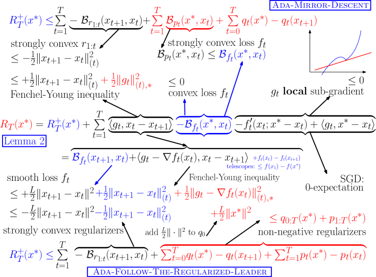
Figure 2: A summary of the proof techniques that incorporate each of the assumptions into regret bounds; see Corollaries B.1–B.5 and Table 2. The identity in the middle is from Section 2.1, whereas the top and bottom bounds on $R_{T}^{+}$ are due to Theorem 3.1. Each arrow shows the transformation of one of the terms, using the stated assumption or technique. The matching terms cancel, and the terms shown in red appear in the final bounds.

In both settings, the regret can be reduced when the losses are strongly convex. Furthermore, in the stochastic optimization setting, the smoothness of the loss is also helpful in decreasing the regret. The next two assumptions capture these conditions.

Assumption 6 (Loss smoothness)

The function $f$ is differentiable and $1$-smooth w.r.t. some norm $\|\cdot\|$.

Assumption 7 (Loss strong convexity)

The losses are 1-strongly convex w.r.t. the regularizers, that is, $\mathcal{B}_{f_{t}}(x^{*},x_{t})\geq\mathcal{B}_{p_{t}}(x^{*},x_{t})$ for $t=1,2,\dots,T$.

Note that if $p_{t},q_{t-1}$ are convex, then it suffices to have $\mathcal{B}_{r_{t}}$ in the condition (rather than $\mathcal{B}_{p_{t}}$). Typically, if $f_{t}$ is strongly convex w.r.t. a norm $\|\cdot\|_{(t)}$, then $p_{t}$ (or $r_{t}$) is set to $\eta\|\cdot\|_{(t)}$ for some $\eta>0$. Again, in stochastic optimization, Assumption 7 simplifies to $\mathcal{B}_{f}(x^{*},x_{t})\geq\mathcal{B}_{p_{t}}(x^{*},x_{t})$, $t=1,2,\dots,T$. Furthermore, if $p_{t}$ is convex, then Assumption 7 implies that $f_{t}$ is convex.

Finally, the results that we recover depend on the assumption that the total regularization, in both Ada-FTRL and Ada-MD, is strongly convex:

Assumption 8 (Strong convexity of regularizers)

For all $t=1,2,\dots,T$, $r_{1:t}$ is $1$-strongly convex w.r.t. some norm $\|\cdot\|_{(t)}$.

Setting / Algorithms	Assumptions	Regret / Expected Stochastic Regret Bound
OO/SO Ada-FTRL	1, 3/4, 5, 8	$\sum_{t=0}^{T}\left(q_{t}(x^{*})-q_{t}(x_{t+1})\right)$ $+\sum_{t=1}^{T}\left(p_{t}(x^{*})-p_{t}(x_{t})\right)+\sum_{t=1}^{T}\frac{1}{2}\|g_{t}\|_{(t),*}^{2}$
OO/SO Ada-MD	2, 3/4, 5, 8	$\sum_{t=0}^{T}\left(q_{t}(x^{*})-q_{t}(x_{t+1})\right)$ $+\sum_{t=1}^{T}\mathcal{B}_{p_{t}}(x^{*},x_{t})+\frac{1}{2}\|g_{t}\|_{(t),*}^{2}$
Strongly-convex OO/SO Ada-MD	2, 3/4, (5), 8, 7	$\sum_{t=0}^{T}\left(q_{t}(x^{*})-q_{t}(x_{t+1})\right)$ $+\sum_{t=1}^{T}\frac{1}{2}\|g_{t}\|_{(t),*}^{2}$
Smooth SO Ada-FTRL	1, 4, 6, 5, 8’	$\frac{1}{2}\|x^{*}\|^{2}+D+\sum_{t=0}^{T}\left(q_{t}(x^{*})-q_{t}(x_{t+1})\right)$ $+\sum_{t=1}^{T}\left(p_{t}(x^{*})-p_{t}(x_{t})\right)+\sum_{t=1}^{T}\frac{1}{2}\|\sigma_{t}\|_{(t),*}^{2}$
Smooth SO Ada-MD	2, 4, 6, 5, 8’	$\frac{1}{2}\|x^{*}-x_{1}\|^{2}+D+\sum_{t=0}^{T}\left(q_{t}(x^{*})-q_{t}(x_{t+1})\right)$ $+\sum_{t=1}^{T}\mathcal{B}_{p_{t}}(x^{*},x_{t})+\frac{1}{2}\|\sigma_{t}\|_{(t),*}^{2}$
Smooth & strongly-convex SO Ada-MD	2, 4, 6, (5), 8’, 7	$\frac{1}{2}\|x^{*}-x_{1}\|^{2}+D+\sum_{t=0}^{T}\left(q_{t}(x^{*})-q_{t}(x_{t+1})\right)$ $+\sum_{t=1}^{T}\frac{1}{2}\|\sigma_{t}\|_{(t),*}^{2}$

Table 2: Recovered and generalized standard results for online optimization (OO) and stochastic optimization (SO); see Corollaries B.1–B.5. A number in parentheses indicates that the assumption is not directly required, but is implied by the other assumptions. In the bounds above, $\sigma_{t}:=g_{t}-\nabla f(x_{t})$, $D:=f(x_{1})-\inf_{\mathcal{X}}f(x)$, and 8’ refers to a slightly modified version of Assumption 8, as described in Corollary B.5. Note that setting $q_{T}=0$ recovers the off-by-one property (McMahan, 2014) in FTRL-Centered vs. FTRL-Prox; Ada-MD exhibits a similar property. For composite-objective Ada-FTRL and Ada-MD, these same bounds apply with $\tilde{q}_{t}$ in place of $q_{t}$ in the summation; see Table 1 and Section 5.

Table 2 provides a summary of the standard results, under different sub-sets of the assumptions above, that are recovered and generalized using our framework. The derivations of these results are provided in the form of three corollaries in Appendix B. Note that the analysis is absolutely modular: each assumption is simply plugged into (23) or (24) to obtain the final bounds, without the need for a separate analysis of Ada-FTRL and Ada-MD for each individual setting. A schematic view of the (standard) proof ideas is given in Figure 2.

5 Composite-objective learning and optimization

Next, we consider the composite-objective online learning setting. In this setting, the functions $f_{t}$, from which the (local sub-)gradients $g_{t}$ are generated and fed to the algorithm, comprise only part of the loss. Instead of $R_{T}(x^{*})$, we are interested in minimizing the regret

$$R_{T}^{(\ell)}(x^{*}):=\sum_{t=1}^{T}f_{t}(x_{t})+\psi_{t}(x_{t})-f_{t}(x^{*})-\psi_{t}(x^{*})=R_{T}(x^{*})+\sum_{t=1}^{T}\psi_{t}(x_{t})-\psi_{t}(x^{*})\,,$$

using the feedback $g_{t}\in\delta f_{t}(x_{t})$, where $\psi_{t}:\mathcal{H}\to\overline{\mathbb{R}}$ are proper functions. The functions $\psi_{t}$ are not linearized, but are passed directly to the algorithm.

Naturally, one can use the $q_{t}$ regularizers to pass the $\psi_{t}$ functions to Ada-FTRL and Ada-MD. Then, we can obtain the exact same bounds as in Table 2 on the composite regret $R^{(\ell)}_{T}(x^{*})$; this recovers and extends the corresponding bounds by Xiao (2009); Duchi et al. (2011, 2010); McMahan (2014). In particular, consider the following two scenarios:

Setting 1: $\psi_{t}$ is known before predicting $x_{t}$.

In this case, we run Ada-FTRL or Ada-MD with $q_{t}=\psi_{t+1}+\tilde{q}_{t},t=0,1,2,\dots,T$ (where $\psi_{T+1}:=0$). Thus, we have the update

$$x_{t+1}\in\operatorname{argmin}_{x\in\mathcal{X}}\ \langle g_{1:t},x\rangle+\psi_{1:t+1}(x)+\tilde{q}_{0:t}(x)+p_{1:t}(x)\,,$$ (9)

for Ada-FTRL, and

$$x_{t+1}\in\operatorname{argmin}_{x\in\mathcal{X}}\ \langle g_{t},x\rangle+\psi_{t+1}(x)+\tilde{q}_{t}(x)+\mathcal{B}_{r_{1:t}}(x,x_{t})\,,$$ (10)

for Ada-MD. Then, we have the following result.

Corollary 5.1.

Suppose that the iterates $x_{1},x_{2},\dots,x_{T+1}$ are given by the Ada-FTRL update (9) or the Ada-MD update (10), and $q_{t},p_{t},$ and $r_{t}$ satisfy Assumption 1 for Ada-FTRL, or Assumption 2 for Ada-MD. Then, under the conditions of each section of Corollaries B.1, B.3 and B.5, the composite regret $R^{(\ell)}_{T}(x^{*})$ enjoys the same bound as $R_{T}(x^{*})$, but with $\sum_{t=0}^{T}\tilde{q}_{t}(x^{*})-\tilde{q}_{t}(x_{t+1})$ in place of $\sum_{t=0}^{T}q_{t}(x^{*})-q_{t}(x_{t+1})$.

Proof 5.2.

By definition, $\sum_{t=0}^{T}\tilde{q}_{t}(x^{*})-\tilde{q}_{t}(x_{t+1})-q_{t}(x^{*})+q_{t}(x_{t+1})=\sum_{t=1}^{T}\psi_{t}(x_{t})-\psi_{t}(x^{*})$. Thus, $R^{(\ell)}_{T}(x^{*})=R_{T}(x^{*})+\sum_{t=0}^{T}\tilde{q}_{t}(x^{*})-\tilde{q}_{t}(x_{t+1})-q_{t}(x^{*})+q_{t}(x_{t+1})$. Upper-bounding $R_{T}(x^{*})$ by the aforementioned corollaries completes the proof.

Setting 2: $\psi_{t}$ is revealed after predicting $x_{t}$, together with $g_{t}$.

In this case, we run Ada-FTRL and Ada-MD with functions $q_{0}=\tilde{q}_{0}$, $q_{t}=\psi_{t}+\tilde{q}_{t},t=1,2,\dots,T$, so that

$$x_{t+1}\in\operatorname{argmin}_{x\in\mathcal{X}}\ \langle g_{1:t},x\rangle+\psi_{1:t}(x)+\tilde{q}_{0:t}(x)+p_{1:t}(x)\,,$$ (11)

for Ada-FTRL, and

$$x_{t+1}\in\operatorname{argmin}_{x\in\mathcal{X}}\ \langle g_{t},x\rangle+\psi_{t}(x)+\tilde{q}_{t}(x)+\mathcal{B}_{r_{1:t}}(x,x_{t})\,,$$ (12)

for Ada-MD. Then, we have the following result, proved in Appendix C.

Corollary 5.3.

Suppose that the iterates $x_{1},x_{2},\dots,x_{T+1}$ are given by the Ada-FTRL update (11) or the Ada-MD update (12), and $q_{t},p_{t},$ and $r_{t}$ satisfy Assumption 1 for Ada-FTRL, or Assumption 2 for Ada-MD. Also, assume that $\psi_{1}(x_{1})=0$ and the $\psi_{t}$ are non-negative and non-increasing, i.e., that $\psi_{1}\geq\psi_{2}\geq\dots\geq\psi_{T+1}:=0$. Then, under the conditions of each section of Corollaries B.1, B.3 and B.5, the composite regret $R^{(\ell)}_{T}(x^{*})$ enjoys the same bound as $R_{T}(x^{*})$, but with $\sum_{t=0}^{T}\tilde{q}_{t}(x^{*})-\tilde{q}_{t}(x_{t+1})$ in place of $\sum_{t=0}^{T}q_{t}(x^{*})-q_{t}(x_{t+1})$.

Remark 5.4.

In both settings, the functions $\psi_{t}$ are passed as part of the regularizers $q_{t}$. Thus, if the $\psi_{t}$ are strongly convex, less additional regularization is needed in Ada-FTRL to ensure the strong convexity of $r_{1:t}$ because $q_{0:t-1}$ will already have some strongly convex components. In addition, in Ada-MD, when the $\psi_{t}$ are convex, the $\mathcal{B}_{p_{t}}$ terms in (8) will be smaller than the $\mathcal{B}_{r_{t}}$ terms found in previous analyses of MD. This is especially useful for implicit updates, as shown in the next section. This also demonstrates another benefit of the generalized Bregman divergence: the $\psi_{t}$, and hence the $p_{t}$, may be non-smooth in general.

6 Implicit-update Ada-MD and non-linearized Ada-FTRL

Other learning settings can be captured using the idea of passing information to the algorithm using the $q_{t}$ functions. This information could include, for example, the curvature of the loss. In particular, consider the composite-objective Ada-FTRL and Ada-MD, and for $t=1,2,\dots,T$, let $\ell_{t}$ be a differentiable loss, $f_{t}=\langle\nabla\ell_{t}(x_{t}),x-x_{t}\rangle$, and $\psi_{t}=\mathcal{B}_{\ell_{t}}(\cdot,x_{t})$. Then, $\ell_{t}=f_{t}+\psi_{t}$, $g_{t}=\nabla f_{t}(x_{t})=\nabla\ell_{t}(x_{t})$, and the composite-objective Ada-FTRL update (11) is equivalent to

$$x_{t+1}\in\operatorname{argmin}_{x\in\mathcal{X}}\ \ell_{1:t}(x)+\tilde{q}_{0:t}(x)+p_{1:t}(x)\,.$$ (13)

Thus, non-linearized FTRL, studied by McMahan (2014), is a special case of Ada-FTRL. With the same $f_{t},\psi_{t}$, the composite-objective Ada-MD update (12) is equivalent to

$$x_{t+1}\in\operatorname{argmin}_{x\in\mathcal{X}}\ \ell_{t}(x)+\tilde{q}_{t}(x)+\mathcal{B}_{r_{1:t}}(x,x_{t})\,,$$ (14)

so the implicit-update MD is also a special case of Ada-MD.

Again, combining Sections 2.1 and 3.1 results in a compact analysis of these algorithmic ideas. In particular, for both updates (13) and (14), the bounds of (23) and (24) apply on the regret in $f_{t}$. Then, moving the terms $\psi_{t}(x^{*})$ to the left turns each bound to a bound on the regret in $\ell_{t}$. Furthermore, the terms $-\psi_{t}(x_{t+1})=-\mathcal{B}_{\ell_{t}}(x_{t+1},x_{t})$ that remained on the right-hand side can be merged with the $-\mathcal{B}_{r_{1:t}}(x_{t+1},x_{t})$ terms. Thus, instead of $r_{0:t}$, it is enough for $r_{1:t}+\ell_{t}$ to be strongly convex w.r.t. the norm $\|\cdot\|_{(t)}$ (see the proofs of Corollaries B.1, B.3 and B.5). This means that if $\ell_{t}$ are strongly convex, then no further regularization is required: $\ell_{1:t}$ is strongly convex, and we get back the well-known logarithmic bounds for strongly-convex FTRL (Follow-The-Leader) and implicit-update MD (Kivinen and Warmuth, 1997; Kulis and Bartlett, 2010; Shalev-Shwartz and Kakade, 2009; Hazan et al., 2007; Orabona et al., 2015; McMahan, 2014). In addition, as mentioned before, convexity of $\ell_{t}$ further reduces the term $\mathcal{B}_{p_{t}}$ in implicit-update MD.

Finally, note that multiple pieces of information can be passed to the algorithm through $q_{t}$. In particular, none of the above interfere with further use of another composite term $\phi_{t}$ and obtaining regret bounds on $\ell_{t}+\phi_{t}$, as discussed in Section 5.

7 Adaptive optimistic learning and variational bounds

The goal of optimistic online learning algorithms (Rakhlin and Sridharan, 2013a, b) is to obtain improved regret bounds when playing against “easy” (i.e., predictable) sequences of losses. This includes algorithms with regret rates that grow with the total “variation”, i.e., the sum of the norms of the differences between pairs of consecutive losses $f_{t}$ and $f_{t+1}$ observed in the loss sequence: the regret will be small if the loss sequence changes slowly (Chiang et al., 2012).

Recently, Mohri and Yang (2016) proposed an interesting comprehensive framework for analyzing adaptive FTRL algorithms for predictable sequences. The framework has also been extended to MD by Kamalaruban (2016). However, despite their generality, the regret analyses of Mohri and Yang (2016) and Kamalaruban (2016) can be strengthened. Specifically, the two analyses do not recover the variation-based results of Chiang et al. (2012) for smooth losses. In addition, their treatment of composite objectives introduces complications, e.g., only applies to Setting 5 of Section 5 where $\psi_{t}$ is known before selecting $x_{t}$.

The flexibility of the framework introduced in this paper allows us to alleviate these and other limitations. In particular, we cast the Adaptive Optimistic FTRL (AO-FTRL) algorithm of Mohri and Yang (2016) as a special case of Ada-FTRL, and obtain a much simpler form of Adaptive Optimistic MD (AO-MD) as a special case of Ada-MD. Then, we strengthen and simplify the corresponding analyses, and recover and extend the results of Chiang et al. (2012). Finally, building on the modularity of our framework, we obtain an adaptive composite-objective algorithm with variational bounds that improves upon the results of Mohri and Yang (2016); Kamalaruban (2016); Chiang et al. (2012); Rakhlin and Sridharan (2013a, b).

7.1 Adaptive optimistic FTRL

Consider the online optimization setting of Section 4 (Assumption 3). Suppose that the losses $f_{1},f_{2},\dots,f_{T}$ satisfy Assumption 5 (e.g., they are convex), and the sequence of points $x_{t+1},t=0,1,2,\dots,T$ is given by

$$x_{t+1}\in\operatorname{argmin}_{x\in\mathcal{X}}\ \langle g_{1:t}+\tilde{g}_{t+1},x\rangle+p_{1:t}(x)+\tilde{q}_{0:t}(x)\,,$$

where $\tilde{g}_{t},t=1,2,\dots,T+1,$ is any sequence of vectors in $\mathcal{H}$. That is, we run Ada-FTRL, but we also incorporate $\tilde{g}_{t+1}$ as a “guess” of the future loss $g_{t+1}$ that the algorithm will suffer. Mohri and Yang (2016) refer to this algorithm as AO-FTRL.

It is easy to see that AO-FTRL is a special case of Ada-FTRL: Define $\tilde{g}_{0}:=0$, and for $t=0,1,\dots,T$, let $q_{t}=\tilde{q}_{t}+\langle\tilde{g}_{t+1}-\tilde{g}_{t},\cdot\rangle$. Then, $q_{0:t}=\tilde{q}_{0:t}+\langle\tilde{g}_{t+1},\cdot\rangle$, so we have

$$x_{t+1}\in\operatorname{argmin}_{x\in\mathcal{X}}\ \langle g_{1:t},x\rangle+p_{1:t}(x)+q_{0:t}(x)\,,$$

which is the Ada-FTRL update with this specific choice of $q_{t}$. Thus, the exact same manipulations as in Corollary B.1 give the following theorem, proved in Appendix D:

Theorem 7.1.

If the losses satisfy Assumption 5, and the regularizers $q_{0}$ and $p_{t},q_{t},t=1,2,\dots,T$, satisfy Assumptions 1 and 8, then the regret of AO-FTRL is bounded as

$$R_{T}(x^{*})\leq \ \sum_{t=0}^{T-1}\left(\tilde{q}_{t}(x^{*})-\tilde{q}_{t}(x_{t+1})\right)+\sum_{t=1}^{T}\left(p_{t}(x^{*})-p_{t}(x_{t})\right)+\sum_{t=1}^{T}\frac{1}{2}\|g_{t}-\tilde{g}_{t}\|_{(t),*}^{2}\,.$$ (15)

This bound recovers Theorems 1 and 2 of Mohri and Yang (2016). Similarly, one could prove parallels of Corollaries B.3 and B.5 for AO-FTRL. Then, the modularity property allows us (as we do in Section 7.4) to apply the composite-objective technique of Section 5 and recover Theorems 3-7 of Mohri and Yang (2016) (and hence their corollaries). Indeed, the resulting analysis simplifies and improves on the analysis of Mohri and Yang (2016) in several aspects: we do not need to separate the cases for FTRL-Prox and FTRL-General, we naturally handle the composite objective case for Settings 5 and 5 while avoiding any complications with proximal regularizers, and do not lose the constant $1/2$ factor. Finally, Theorem 3.1 allows us to improve on the results of Chiang et al. (2012), as we show next.

7.2 Adaptive optimistic MD

Interestingly, we can use the exact same assignment $q_{t}=\tilde{q}_{t}+\langle\tilde{g}_{t+1}-\tilde{g}_{t},\cdot\rangle$ in Ada-MD. This results in the update

$$x_{t+1}\in\operatorname{argmin}_{x\in\mathcal{X}}\ \langle g_{t}+\tilde{g}_{t+1}-\tilde{g}_{t},x\rangle+\tilde{q}_{t}(x)+\mathcal{B}_{r_{1:t}}(x,x_{t})\,.$$

Applying the same argument as in Theorem 7.1, one can show that this optimistic MD algorithm enjoys the regret bound of (15) with the $p_{t}(x^{*})-p_{t}(x_{t})$ terms replaced by $\mathcal{B}_{p_{t}}(x^{*},x_{t})$. This gives an optimistic MD algorithm with only one projection in each round; all other formulations (Kamalaruban, 2016; Rakhlin and Sridharan, 2013b, a; Chiang et al., 2012) require two MD steps in each round. This new formulation has the potential to greatly simplify the previous analyses of variants of optimistic MD. In particular, handling implicit updates or composite terms is a matter of including them in $\tilde{q}_{t}$. Especially, unlike Kamalaruban (2016), we can handle Setting 5 in the exact same way as we do in the AO-FTRL case (see Section 7.4). Further exploration of the properties of this new class of algorithms is left for for future work.

7.3 Variation-based bounds for online learning

Suppose that the losses $f_{t}$ are differentiable and convex, and define $f_{0}:=0$. For any norm $\|\cdot\|$, we define the total variation of the losses in $\|\cdot\|_{*}^{2}$ as

$$D_{\|\cdot\|}:=\sum_{t=1}^{T}\sup_{x\in\mathcal{X}}\|\nabla f_{t}(x)-\nabla f_{t-1}(x)\|_{*}^{2}\,.$$ (16)

Chiang et al. (2012) use an optimistic MD algorithm to obtain regret bounds of order $O(\sqrt{D_{2}})$, where $D_{2}=D_{\|\cdot\|_{2}}$, for linear as well as smooth losses.

If the losses are linear, i.e., $f_{t}=\langle g_{t},\cdot\rangle$, then Theorem 7.1 immediately recovers the result of Chiang et al. (2012, Theorem 8). In particular, let $\tilde{q}_{0}=(1/2\eta)\|.\|_{2}^{2}$, and for $t=1,2,\dots,T$, let $p_{t}=\tilde{q}_{t}=0$, $\|.\|_{(t)}^{2}=\eta\|.\|_{2}^{2}$, and $\tilde{g}_{t}=g_{t-1}$. Then (15) gives the regret bound $(\eta/2)\|x^{*}\|_{2}^{2}+(1/(2\eta))D_{2}$. If $\|x\|_{2}\leq 1$ and we set $\eta$ based on $D_{2}$ (as Chiang et al. assume), we obtain their $O(\sqrt{D_{2}})$ bound.

If the losses are not linear but are $L$-smooth, then by the combination of Section 2.1 and Theorem 3.1, we still obtain $\sqrt{D_{\|\cdot\|}}$-bounds, as Chiang et al. (2012, Theorem 10) also obtain for $D_{2}$. This is because, unlike the analysis of Mohri and Yang (2016), we retain the negative terms $-B_{r_{1:t}}(x_{t+1},x_{t})$ (essentially having the same role as the $B_{t}$ terms of Chiang et al., 2012) in the regret bound. Combined with ideas from Lemma 13 of Chiang et al. (2012), this gives the desired bounds in terms of $D_{\|\cdot\|}$, proved in Appendix D:

Theorem 7.2.

Consider the conditions of Theorem 7.1, and further suppose that the losses $f_{t}$ are convex and $L$-smooth w.r.t. a norm $\|\cdot\|$. For $t=1,2,\dots,T+1$, let $\eta_{t}>0$, and suppose that Assumption 8 holds with $\|\cdot\|_{(t)}^{2}=\eta_{t}\|\cdot\|^{2}$. Further assume that $q_{0}\geq 0$, $p_{t},q_{t}\geq 0,t\geq 1$, and $\eta_{t}\eta_{t+1}\geq 8L^{2},t=1,2,\dots,T$. Then, AO-FTRL with $\tilde{g}_{t}=g_{t-1}$ satisfies

$$R_{T}(x^{*})\leq \ \tilde{q}_{0:T}(x^{*})+p_{1:T}(x^{*})+2\sum_{t=1}^{T}\frac{1}{\eta_{t}}\max_{x\in\mathcal{X}}\|\nabla f_{t}(x)-\nabla f_{t-1}(x)\|_{*}^{2}\,.$$ (17)

Letting $\eta_{t}=\eta=\sqrt{D_{\|\cdot\|}}$, and $\tilde{q}_{0}=\eta\|\cdot\|^{2},\tilde{q}_{t},p_{t}=0,t\geq 1,$ generalizes the $O(\sqrt{D_{2}})$ bound of Chiang et al. (2012) to any norm (under the same assumption they make, that $D_{\|\cdot\|}\geq 8L^{2}$). In the next section, we provide an algorithm that does not need prior knowledge of $D_{\|\cdot\|}$.

7.4 Adaptive optimistic composite-objective learning with variational bounds

Next, we provide a simple analysis of the composite-objective version of AO-FTRL, and obtain variational bounds in terms of $D_{\|\cdot\|}$ for composite objectives with smooth $f_{t}$. We focus on Setting 5; similar results are immediate for Setting 5. Consider the update

$$x_{t+1}\in\operatorname{argmin}_{x\in\mathcal{X}}\ \langle g_{1:t}+\tilde{g}_{t+1},x\rangle+\psi_{1:t}(x)+p_{1:t}(x)+\tilde{q}_{0:t}(x)\,,$$ (18)

that is, the composite-objective AO-FTRL algorithm. Then we have the following corollary of Theorem 7.1.

Corollary 7.3.

Suppose that $\psi_{t},t=1,2,\dots,T$, satisfy the conditions of Corollary 5.3, and $\tilde{q}_{0}$ and $p_{t},\tilde{q}_{t},t\geq 1,$ are non-negative. Let $q_{0}=\tilde{q}_{0}+\langle\tilde{g}_{1},\cdot\rangle$ and $q_{t}=\tilde{q}_{t}+\psi_{t}+\langle\tilde{g}_{t+1}-\tilde{g}_{t},\cdot\rangle$. Suppose that $q_{0}$, $p_{t},q_{t},t\geq 1$ satisfy Assumptions 1 and 8, and $f_{t},t\geq 1$ satisfy Assumption 5. Then, composite-objective AO-FTRL (update (18)) satisfies

$$R^{(\ell)}_{T}(x^{*})\leq \ \tilde{q}_{0:T-1}(x^{*})+p_{1:T}(x^{*})+\sum_{t=1}^{T}\frac{1}{2}\|g_{t}-\tilde{g}_{t}\|_{(t),*}^{2}\,.$$

Proof 7.4.

Starting as in Corollary 5.3, defining $\tilde{g}_{0}=0$, and noting that $0=q_{0}-\tilde{q}_{0}-\langle\tilde{g}_{1},\cdot\rangle$,

$$R^{(\ell)}_{T}(x^{*})\leq \ R_{T}(x^{*})+\sum_{t=0}^{T}q_{t}(x_{t+1})-\tilde{q}_{t}(x_{t+1})+\tilde{q}_{t}(x^{*})-q_{t}(x^{*})-\langle\tilde{g}_{t+1}-\tilde{g}_{t},x_{t+1}-x^{*}\rangle\,.$$

Proceeding as in Theorem 7.1 completes the proof.

The bounds of Mohri and Yang (2016) for Setting 5 correspond to the non-proximal FTRL case. As such, one has to set the step-size sequences according to the Dual-Averaging AdaGrad recipe (c.f. Table 1), which requires an additional regularization of $\tilde{q}_{0}=\sqrt{\delta}\|\cdot\|_{2}^{2}$. In contrast, in FTRL-Prox, $\tilde{q}_{0}=0$. This $\delta$ value makes Dual-Averaging AdaGrad non-scale-free, while FTRL-Prox is scale-free (i.e., the $x_{t}$ are independent of the scaling of $f_{t}$). Our analysis avoids this problem by the early separation of the proximal ($p_{t}$) and non-proximal regularizers ($q_{t}$) in Ada-FTRL. In particular, $p_{t},\tilde{q}_{t}$ in Corollary 7.3 can be set as $\tilde{q}_{t}=0$ and $p_{t}=\frac{\eta_{t}-\eta_{t-1}}{2}\|x-x_{t}\|^{2}$ with $\eta_{t}=\eta\sqrt{\sum_{s=1}^{t}\|g_{s}-\tilde{g}_{s}\|_{*}^{2}},\eta>0$ for $t=1,2,\dots,T$. This gives composite-objective AO-FTRL-Prox, a scale-free adaptive optimistic algorithm for Setting 5.

In addition, using Theorem 7.2, we can obtain a variational bound for composite-objective optimistic FTRL-Prox (proved in Appendix D), which was not available through the analysis of Mohri and Yang (2016) even under Setting 5:

Corollary 7.5.

Let $\psi_{t},t=1,2,\dots,T$, be convex and satisfy the conditions of Corollary 5.3. Further assume that $f_{t}$ are convex and $L$-smooth w.r.t. some norm $\|\cdot\|$. Suppose that $\mathcal{X}$ is closed, and let $R^{2}=\sup_{x,y\in\mathcal{X}}\|x-y\|^{2}<+\infty$ be the diameter of $\mathcal{X}$ measured in $\|\cdot\|$. Define $\eta=2/R$. Suppose we run composite-objective AO-FTRL (update (18)) with the following parameters: $\tilde{q}_{0}=0$, and for $t=1,2,\dots,T$, $\tilde{g}_{t}=g_{t-1}$, $\tilde{q}_{t}=0$, and $p_{t}=\frac{\eta_{t}-\eta_{t-1}}{2}\|x-x_{t}\|^{2}$, where $\eta_{0}=0$ and $\eta_{t}=4RL^{2}+\eta\sqrt{\sum_{s=1}^{t}\|g_{s}-\tilde{g}_{s}\|_{*}^{2}}$ for $t\geq 1$. Then,

$$R^{(\ell)}_{T}(x^{*})\leq \ 2R^{3}L^{2}+R+2R\sqrt{2D_{\|\cdot\|}}=O\left(R\sqrt{D_{\|\cdot\|}}\right)\,.$$ (19)

Note that the learning rate $\eta_{t}$ is bounded from below (by $4RL^{2}$), which is essential in the algorithm to achieve a combination of the best properties of Mohri and Yang (2016), Chiang et al. (2012), and Rakhlin and Sridharan (2013a, b): First, like Mohri and Yang (2016), we allow the use of composite-objectives. Second, similarly to Chiang et al. (2012) (but unlike Mohri and Yang 2016; Rakhlin and Sridharan 2013a, b) our bound applies to the variation of general convex smooth functions, and is still optimal when $L=0$ (e.g., Corollary 2 of Rakhlin and Sridharan 2013b). Third, we do not need the knowledge of $D_{\|\cdot\|}$ (required by Chiang et al. 2012) to set the step-sizes, and avoid the regret penalty of using a doubling trick (as done by Rakhlin and Sridharan (2013a)). Fourth, in the practically interesting case of a composite L1 penalty ($\psi_{t}=\alpha_{t}\|\cdot\|_{1}$), FTRL-Prox, which is the basis of our algorithm, gives sparser solutions (McMahan, 2014) than MD, which is the basis of the algorithms of Chiang et al. (2012) and Rakhlin and Sridharan (2013b). Fifth, when $L=0$, the algorithm is scale-free (unlike Mohri and Yang 2016 and Rakhlin and Sridharan 2013a). Finally, the results apply to the variation measured in any norm.

8 Application to non-convex optimization

In this section, we collect some results related to applying online optimization methods to non-convex optimization problems. This is another setting where the strength of our derivations is apparent: As we shall see, without any extra work, the results imply and extend previous results.

Central to this extension is the decomposition of assumptions in our analysis: we are not using the convexity of $f_{t}$ in Section 2.1 or Theorem 3.1, but only at the very last stage of the analysis, where convexity can ensure that Assumption 5 holds. Thus, the analysis easily extends to non-convex optimization problems where Assumption 5 either holds or could be replaced by another technique at the final stage of the analysis. In the rest of this section, we explore such classes of non-convex problems, which are also related to the Polyak-Łojasiewicz (PL) condition used in the non-convex optimization and learning community. For background and a summary of related work, consult Karimi et al. (2016).

8.1 Stochastic optimization of star-convex functions

First, we explore the class of non-convex functions for which Assumption 5 directly holds. As it turns out, this is a much larger class of functions than convex functions. In particular, consider the so-called “star-convex” functions (Nesterov and Polyak, 2006):

Definition 8.1 (Star-convex function).

A function $f$ is star-convex at a point $x^{*}$ if and only if $x^{*}$ is a global minimizer of $f$, and for all $\alpha\in[0,1]$ and all $x\in\textnormal{dom}(f)$:

$$f(\alpha x^{*}+(1-\alpha)x)\leq\alpha f(x^{*})+(1-\alpha)f(x)\,.$$ (20)

A function is said to be star-convex when it is star-convex at some of its global minimizers.

The name “star-convex” comes from the fact that the sub-level sets $L_{\beta}=\{x\,:\,f(x)\leq\beta\}$ of a function $f$ that is star-convex at $x^{*}$ are star-shaped with center $x^{*}$ (recall that a set $U$ is star-convex with center $x$ if for any $y\in U$, the segment between $x$ and $y$ is included in $U$). However, note that there are functions whose sub-level sets are star-convex that are themselves not star-convex. In particular, functions that are increasing along the rays (IAR) started from their global minima have star-shaped sub-level sets and vice versa, but some of these functions (e.g., $f(x)=\sqrt{|x|}$, $x\in\mathbb{R}$) is clearly not star-convex. Recall that quasi-convex functions are those whose sub-level sets are convex. In one dimension a star-convex function is thus also necessarily quasi-convex. However, clearly, there are star-convex functions (such as $x\mapsto|x|\mathbb{I}\{|x|\leq 1\}+2|x|\mathbb{I}\{|x|>1\}$, $x\in\mathbb{R}$) that are not convex and in multiple dimensions there are star-convex functions that are not quasi-convex (e.g., $x\mapsto\|x\|^{2}g(\frac{x}{\|x\|_{2}^{2}})$ where $g(u)$ is, say, the sine of the angle of $u$ with the unit vector $e_{1}$).

Star-convex functions arise in various optimization settings, often related to sums of squares (Nesterov and Polyak, 2006; Lee and Valiant, 2016). It is easy to see from the definitions that the set of star-convex functions is closed under nonsingular affine domain transformations, addition (of functions having the same center) and multiplication by nonnegative constants. Further, for $x\in\mathbb{R}^{d}$, $x\mapsto\prod_{i}|x_{i}|^{p_{i}}$ is star-convex (at zero) whenever $\sum_{i}p_{i}\geq 1$. For further properties and examples see Lee and Valiant (2016).

We can immediately see that Assumption 5 holds for star-convex functions:

Lemma 8.2 (Non-negative Bregman divergence for star-convex functions).

Let $f$ be a directionally differentiable function with global optimum $x^{*}$. Then, $f$ is star-convex at $x^{*}$ if and only if for all $x\in\mathcal{H}$,

$$\mathcal{B}_{f}(x^{*},x)\geq 0\,.$$

Proof 8.3.

Both directions are routine. For illustration we provide the proof of the forward direction. Assume without loss of generality that $x^{*}=0$ and $f(x^{*})=0$. Then star-convexity at $x^{*}$ is equivalent to having $f(\alpha x)\leq\alpha f(x)$ for any $x$ and $\alpha\in[0,1]$. Further, $\mathcal{B}_{f}(x^{*},x)\geq 0$ is equivalent to $-f(x)-f^{\prime}(x;-x)\geq 0$. Now, $f^{\prime}(x;-x)=\lim_{\alpha\downarrow 0}\frac{f(x+\alpha(-x))-f(x)}{\alpha}$. Under star-convexity, $f(x+\alpha(-x))=f((1-\alpha)x)\leq(1-\alpha)f(x)$. Hence, $f^{\prime}(x;-x)\leq\lim_{\alpha\downarrow 0}\frac{(1-\alpha)f(x)-f(x)}{\alpha}=-f(x)$.

Thus, Corollaries B.3 and B.5 apply to star-convex functions. In other words:

• For stochastic optimization of directionally-differentiable star-convex functions in Hilbert spaces, Ada-FTRL and Ada-MD converge to the global optimum with the same rate as they converge for convex functions (including fast rates due to other assumptions, e.g., smoothness).

Of course, a similar result holds for the online setting, too, but in this case the assumption that each $f_{t}$ is star-convex w.r.t. the same center $x^{*}$ becomes restrictive.

Remark 8.4.

Since the rate of regret depends on the norm of the gradients $g_{t}$, to get fast rates one needs to control these norms. This is trivial if $f$ is Lipschitz-continuous. However, some star-convex functions are not Lipschitz, even arbitrarily close to the optima (e.g., $f(x,y)=(\sqrt{|x|}+\sqrt{|y|})^{2}$). For such functions, Lee and Valiant (2016) propose alternative methods to gradient descent. However, it seems possible to control the norms in these settings using additional regularization (as in the normalized gradient descent method); see, e.g., the work of Hazan et al. 2015, and the recent work of Levy (2017). Exploring this idea is left for future work.

8.2 Beyond star-convex functions

Inspecting our proofs we may notice that Assumption 5 is unnecessarily restrictive: to maintain the same rate of growth for regret, it suffices for the sum of Bregman divergences to grow with the same rate as the rest of the bound, rather than being negative and hence dropped. This extends all of our results to another interesting class of non-convex functions which generalize star-convexity:

Definition 8.5 ($\tau$-star-convexity, Hardt et al. (2016)).

Let $f$ be a directionally differentiable function $f$ with global optimum $x^{*}$. Then $f$ is $\tau$-star-convex on a set $\mathcal{X}$ at $x^{*}\in\mathcal{H}$ if there is $\tau>0$ such that for all $x\in\mathcal{X}\cap\textnormal{dom}(f)$,

$$\tau(f(x)-f(x^{*}))\leq-f^{\prime}(x;x^{*}-x)\,.$$ (21)

Note that by Lemma 8.2, star-convexity corresponds to the case when $\tau=1$. Hardt et al. (2016) demonstrated that an objective function that arises naturally in the identification of certain class of linear systems is $\tau$-star-convex with some $\tau>0$. For differentiable functions, (21) is equivalent to $f(x)-f(x^{*})\leq\frac{1}{\tau}\langle\nabla f(x),x-x^{*}\rangle$, so it is a simple generalization of the linear upper bound one typically uses to reduce online convex optimization to online linear optimization. Therefore, any regret bound that is proved via upper bounding linearized losses automatically extends to $\tau$-star-convex functions. However, in general, it may require substantial work to identify what assumptions are used exactly in proving an upper bound on the linearized loss (e.g., Hardt et al., 2016 reproved the convergence guarantees for smooth SGD). The next lemma shows that our techniques can automatically separate the effects of different assumptions and provide fast regret rates under appropriate circumstances.

Lemma 8.6 (Basic regret bound under $\tau$-star-convexity).

Let $f$ be locally directionally differentiable and $\tau$-star-convex on a set $\mathcal{X}$ at $x^{*}$, $f_{1}\dots=f_{T}=f$. Then, for all $x_{t}\in\mathcal{X}\cap\textnormal{dom}(f_{t})$ and $g_{t}\in\mathcal{H}$ ($t=1,2,\dots,T$),

$$R_{T}(x^{*})\leq\frac{1}{\tau}\left(R_{T}^{+}(x^{*})+\sum_{t=1}^{T}\langle g_{t},x_{t}-x_{t+1}\rangle+\delta_{t}\right)\,.$$

Proof 8.7.

The proof can be derived from the right-hand side of (2), but a shorter direct proof is also available: Add and subtract $\langle g_{t},x^{*}-x_{t}\rangle$ to the right-hand side of (21). Noticing that $-f^{\prime}(x_{t};x^{*}-x_{t})+\langle g_{t},x^{*}-x_{t}\rangle=\delta_{t}$, summing up and using the definition $R_{T}^{+}(x^{*})=\sum_{t}\langle g_{t},x_{t+1}-x^{*}\rangle$ gives the result.

Now since the regret was bounded through the expression in the parentheses of the previous display, Corollaries B.3 and B.5 apply. In other words:

• For stochastic optimization of directionally-differentiable $\tau$-star-convex functions in Hilbert spaces, Ada-FTRL and Ada-MD enjoy $1/\tau$-times the same regret as when they are applied to linearized loss functions (including fast rates due to other assumptions, e.g., smoothness).

In the convex case the strong convexity of the losses (Assumption 7) implied that their Bregman divergences are nonnegative (Assumption 5). The natural generalization of this leads to the following definition:

Definition 8.8 ($\tau$-star-strong-convexity).

Let $f$, $r$ be directionally differentiable and let $x^{*}$ be a global minimum of $f$. Then, $f$ is $\tau$-star-strongly-convex w.r.t. $r$ if $S:=\textnormal{dom}(f)\cap\textnormal{dom}(r)$ is non-empty and there exists $\tau>0$ such that for all $x\in S$ and some minimizer $x^{*}$ of $f$,

$$\tau(f(x)-f(x^{*}))\leq-f^{\prime}(x;x^{*}-x)-\mathcal{B}_{r}(x^{*},x)\,.$$ (22)

Replacing $\tau$-star-convexity with $\tau$-star-strong-convexity gives the following analogue of Lemma 8.6:

Lemma 8.9 (Basic regret bound under $\tau$-star-strong-convexity).

Let $f$, $r$ be locally directionally differentiable. Assume that $f$ is $\tau$-star-strongly-convex w.r.t. $r$ at $x^{*}$ on a set $\mathcal{X}$. Then, for all $x_{t}\in\mathcal{X}\cap\textnormal{dom}(f_{t})\cap\textnormal{dom}(r)$ and $g_{t}\in\mathcal{H}$ ($t=1,2,\dots,T$),

$$R_{T}(x^{*})\leq\frac{1}{\tau}\left(R_{T}^{+}(x^{*})+\sum_{t=1}^{T}\langle g_{t},x_{t}-x_{t+1}\rangle+\delta_{t}-\mathcal{B}_{r}(x^{*},x_{t})\right)\,.$$

Proof 8.10.

The proof follows the same step as that of Lemma 8.6, except that we need to use (22) instead of (21).

It follows that the same manipulations as in Corollaries B.3 and B.5 imply:

• For stochastic optimization of directionally-differentiable $\tau$-star-strongly-convex functions in Hilbert spaces, Ada-FTRL and Ada-MD converge to the global optimum with $1/\tau$-times the same rate as they converge for strongly convex functions.

It appears that $\tau$-star-strong-convexity is related to the Polyak-Łojasiewicz (PL) inequality. Recall that a differentiable function $f$ satisfies the PL inequality with constant $\mu>0$ if

$$\mu(f(x)-f(x^{*}))\leq\frac{1}{2}\|\nabla f(x)\|_{2}^{2}\,,$$

where $x^{*}$ is a global minimizer of $f$. Proposed independently and simultaneously by Polyak (1963) and Łojasiewicz (1963), the PL inequality appears to play a fundamental role in the study of incremental gradient algorithms (see Karimi et al. 2016 and the references therein). As star-convexity, the PL inequality can also be satisfied by non-convex functions, partly explaining the prominent role it plays in the analysis of gradient methods. We can see that $\tau$-star-strong-convexity implies the PL inequality when $r$ is the squared Euclidean norm:

Lemma 8.11 (PL is implied by star-strong-convexity).

Let $r(x)=\frac{1}{2}\|x\|_{2}^{2}$ and let $f$ be differentiable. If $f$ is $\tau$-star-strongly-convex w.r.t. $r$, then $f$ also satisfies the PL inequality with $\mu=\tau$.

Proof 8.12.

Assume that $f$ satisfies (22). We have

$$-f^{\prime}(x;x-x^{*})=\langle\nabla f(x),x^{*}-x\rangle\leq\frac{1}{2}\left(\|\nabla f(x)\|^{2}+\|x^{*}-x\|^{2}\right)\,,$$

where the second step follows from the Fenchel-Young inequality. As it is well known, $B_{r}(x,y)=\frac{1}{2}\|x-y\|^{2}$. Thus, (22) implies that $\tau(f(x)-f(x^{*}))\leq\frac{1}{2}\|\nabla f(x)\|_{2}^{2}$.

Finally, note that the results above do not preclude the use of other algorithmic ideas, such as implicit-update, non-linearized, or composite-objective learning; the same extensions of Corollaries B.3 and B.5, as discussed in Sections 5 and 6, apply here as well. In addition, there are interesting classes of non-convex problems other than the PL class; see, e.g., Karimi et al. (2016). A direction for future work is to explore whether these classes relate to specific conditions on Bregman divergences, and whether similar convergence results for general adaptive optimization are also possible under these function classes.

9 Discussion

In this section we compare the results obtained in this paper to the previous attempts at unified analysis of adaptive FTRL and MD. A starting point of our work was the unifying treatment of online learning algorithms by McMahan (2014), as well as the generalized adaptive FTRL analysis of Orabona et al. (2015).

9.1 Comparison to the analysis of McMahan (2014)

McMahan (2014) also studied a unified, modular analysis of MD and FTRL algorithms (albeit with different modules), assuming that the regularizers $p_{t},q_{t},r_{t}$ are convex, non-negative, and satisfy Assumption 8. Ada-FTRL and Ada-MD encompass all of the algorithms they considered. In particular, their Theorems 1 and 2 are special cases of Corollary B.1 (recall that non-linearized FTRL, and in particular strongly-convex FTRL, are also special cases of Ada-FTRL; see Section 6). In addition, our analysis applies more generally to infinite-dimensional Hilbert spaces, our presentation of Ada-FTRL encompasses a larger set of algorithms, the relaxed assumptions under which we analyzed Ada-FTRL and Ada-MD remove certain practical limitations that existed in the work of McMahan (2014), and our analysis captures a wider range of learning settings. We discuss these improvements below.

Importantly, McMahan (2014) also provides a reduction from MD to a version of FTRL-Prox. This, in particular, illuminates important differences between MD and FTRL in composite-objective learning. We refer the reader to Section 6 of their paper. We decided to keep the presentation of the two algorithms separate to facilitate the relaxation of the assumptions on the regularizers; see Assumptions 1 and 2 and the discussion below.

9.1.1 Relaxing the assumptions on the regularizers

A central part of the modularity of our analysis comes from the flexibility of Assumptions 1 and 2 on the regularizers of Ada-FTRL and Ada-MD. In particular, unlike McMahan (2014), we do not assume that the individual regularizers $p_{t},q_{t},r_{t}$ are non-negative or convex.

This relaxation provides two benefits. First, with the non-negativity restriction removed, we can add arbitrary, possibly linear, components to the regularizers. As we showed above, this resulted in a simple recovery and analysis of optimistic FTRL and a new class of optimistic MD algorithms (Section 7), as well as a straightforward recovery of implicit and non-linearized updates, even for non-convex functions (Section 6).

Second, with the convexity assumption removed, Ada-FTRL and Ada-MD can accommodate algorithmic ideas such as non-decreasing regularization. For example, AdaDelay (Sra et al., 2016), an instance of Ada-MD, uses $r_{1:t}=\eta_{t}\|\cdot\|^{2}$, but $\eta_{t}$ is not guaranteed to be non-decreasing, i.e., $r_{t}$ could be negative and non-convex (while $r_{0:t}$ still remains convex for all $t$). Now, note that MD and FTRL-Prox are closely related. Particularly, if $p_{t}$ are themselves Bregman divergences (as in proximal AdaGrad), then FTRL-Prox and MD have identical regret bounds. Therefore, the techniques of Sra et al. (2016) for controlling the regularizer terms in the bound could be naturally applied, almost with no modification, to an FTRL-Prox version of AdaDelay. This extension to FTRL-Prox is interesting since, as mentioned before, composite FTRL-Prox with an L1 penalty tends to produce sparser results compared to Ada-MD (McMahan, 2014, Section 6). Thus, while this variant of FTRL-Prox is a special case of Ada-FTRL (e.g., Corollary B.1 applies), it was not clear how to analyze this algorithm under the assumptions made by McMahan (2014).

Finally, the choice to separate the proximal and non-proximal regularizers in Ada-FTRL provides certain conveniences. In particular, the $q_{t}$ terms can take the role of incorporating information (such as composite terms) into Ada-FTRL, while the proximal part $p_{t}$ remains intact. This precludes the need to provide a separate analysis for FTRL-Prox every time the structure of information changes (e.g., when implicit updates are added). Thus, unlike Section 5 of McMahan (2014), we did not need to provide a separate analysis (their Theorem 10) for composite-objective FTRL-Prox. We also avoided the complications with composite optimistic FTRL-Prox as in Mohri and Yang (2016); see Section 7.

9.1.2 The regret decomposition and analysis of new learning settings

In comparison to McMahan (2014), the analysis we provided exhibits much flexibility across learning settings. In particular, the regret decomposition given by Lemma 2.1 enabled us to accommodate a wide range of learning settings, and separate the effect of the learning setting from the forward regret of the algorithm. Building on this, for example, we provided a clean analysis of variational and variance-dependent bounds for smooth losses (and generalized them to adaptive algorithms). In addition, by encapsulating the effect of loss convexity into Assumption 5, we could generalize the analysis to certain non-convex classes.

9.2 Comparison to the analysis of Orabona et al. (2015)

Orabona et al. (2015) study a special case of Ada-FTRL, where $p_{t}\equiv 0$ and Assumption 8 holds. The main result of Orabona et al. (2015), i.e., their Lemma 1, can be though of as playing the same role as (23). We emphasize, however, that their Lemma 1 is a quite general result. For example, with a few algebraic operations we could recover a special case of Theorem 3.1 from their Lemma 1, by setting $z_{t}=0$ and moving the linear components to their $f_{t}$ functions. Nevertheless, our analysis extends the work of Orabona et al. (2015) to infinite-dimensional Hilbert-spaces, to FTRL-Prox algorithms, and to Ada-MD. Furthermore, we demonstrated a principled way of mixing algorithmic ideas and incorporating information from the learning setting into FTRL and MD using the $q_{t}$ functions. Finally, the comments of Section 9.1.2 apply.

Importantly, the authors also provide a compact analysis of the Vovk-Azoury-Warmuth algorithm, as well as online binary classification algorithms. These results are essentially obtained from combining their Lemma 1 with interesting regret decompositions other than the one we presented in Lemma 2.1. It seems possible to combine their regret decompositions with our analysis to extend their result to Ada-MD algorithms, and to obtain refined bounds for smooth losses. We leave this direction for future work.

10 Conclusion and future work

We provided a generalized, unified and modular framework for analyzing online and stochastic optimization algorithms, and demonstrated its flexibility on several existing, as well as new, algorithms and learning settings. Our framework can be used together with other algorithmic ideas and learning settings, e.g., adaptive delayed-feedback algorithms like AdaDelay (Sra et al., 2016), but results related to this where out of the scope of this work. There are many interesting questions related to non-convex optimization; while we showed that our results extend to the so-called $\tau$-star(-strongly)-convex functions, which have already found some applications, it remains to be seen whether they also extend to other settings, such as optimization of quasi-convex functions, or functions that satisfy the Polyak-Łojasiewicz inequality. Exploring these and other applications of this framework is left for future work.

We would like to thank the anonymous reviewers for several insightful comments that helped improve the quality of the paper. This work was supported by Amii (formerly AICML) and NSERC.

Appendix A Proof of the regret decomposition Lemma 2.1

Proof A.1.

By definition,

$$f_{t}(x_{t})-f_{t}(x^{*}) =-\mathcal{B}_{f_{t}}(x^{*},x_{t})-f^{\prime}(x_{t};x^{*}-x_{t})$$

$$=\langle g_{t},x_{t}-x^{*}\rangle-\mathcal{B}_{f_{t}}(x^{*},x_{t})+\delta_{t}$$

$$=\langle g_{t},x_{t+1}-x^{*}\rangle+\langle g_{t},x_{t}-x_{t+1}\rangle-\mathcal{B}_{f_{t}}(x^{*},x_{t})+\delta_{t}\,.$$

Summing over $t$ completes the proof.

Appendix B Formal statements and proofs for the standard results described in Table 2

Putting Lemma 2.1 and Theorem 3.1 together, for Ada-FTRL we obtain

$$R_{T}(x^{*})\leq \ -\sum_{t=1}^{T}\mathcal{B}_{f_{t}}(x^{*},x_{t})+\sum_{t=0}^{T}\left(q_{t}(x^{*})-q_{t}(x_{t+1})\right)+\sum_{t=1}^{T}\left(p_{t}(x^{*})-p_{t}(x_{t})\right)$$

$$\ -\sum_{t=1}^{T}\mathcal{B}_{r_{1:t}}(x_{t+1},x_{t})+\sum_{t=1}^{T}\langle g_{t},x_{t}-x_{t+1}\rangle+\sum_{t=1}^{T}\delta_{t}\,,$$ (23)

whereas for Ada-MD,

$$R_{T}(x^{*})\leq \ -\sum_{t=1}^{T}\mathcal{B}_{f_{t}}(x^{*},x_{t})+\sum_{t=0}^{T}\left(q_{t}(x^{*})-q_{t}(x_{t+1})\right)+\sum_{t=1}^{T}\mathcal{B}_{p_{t}}(x^{*},x_{t})$$

$$\ -\sum_{t=1}^{T}\mathcal{B}_{r_{1:t}}(x_{t+1},x_{t})+\sum_{t=1}^{T}\langle g_{t},x_{t}-x_{t+1}\rangle+\sum_{t=1}^{T}\delta_{t}\,.$$ (24)

Next we prove the concrete regret bounds, given in Table 2, based on the above. A schematic view of the proof ideas is given in Figure 2.

Corollary B.1.

Consider the “Online Optimization” setting (Assumption 3), using Ada-FTRL (under Assumption 1) or Ada-MD (under Assumption 2). Suppose that Assumptions 5 and  8 hold. Then,

1. the regret of Ada-MD is bounded as

   $$R_{T}(x^{*})\leq \ \sum_{t=0}^{T}\left(q_{t}(x^{*})-q_{t}(x_{t+1})\right)+\sum_{t=1}^{T}\mathcal{B}_{p_{t}}(x^{*},x_{t})+\sum_{t=1}^{T}\frac{1}{2}\|g_{t}\|_{(t),*}^{2}\,;$$

2. the regret of Ada-FTRL is bounded as

   $$R_{T}(x^{*})\leq \ \sum_{t=0}^{T}\left(q_{t}(x^{*})-q_{t}(x_{t+1})\right)+\sum_{t=1}^{T}\left(p_{t}(x^{*})-p_{t}(x_{t})\right)+\sum_{t=1}^{T}\frac{1}{2}\|g_{t}\|_{(t),*}^{2}\,;$$

3. under Assumption 7, the regret of Ada-MD is bounded as

   $$R_{T}(x^{*})\leq \ \sum_{t=0}^{T}\left(q_{t}(x^{*})-q_{t}(x_{t+1})\right)+\sum_{t=1}^{T}\frac{1}{2}\|g_{t}\|_{(t),*}^{2}\,.$$

Proof B.2.

Note that by Assumption 3, we have

$$\delta_{t}\leq 0\,,$$ (25)

for all $t=1,2,\dots,T$. In addition, by the Fenchel-Young inequality and Assumption 8,

$$\langle g_{t},x_{t}-x_{t+1}\rangle\leq \ \frac{1}{2}\|x_{t}-x_{t+1}\|_{(t)}^{2}+\frac{1}{2}\|g_{t}\|_{(t),*}^{2}$$

$$\leq \ \mathcal{B}_{r_{1:t}}(x_{t+1},x_{t})+\frac{1}{2}\|g_{t}\|_{(t),*}^{2}\,.$$ (26)

Putting (25), (26), and Assumption 5 into (23) and (24) and cancelling out the matching terms proves (i) and (ii). Finally, to prove (iii), we use Assumption 7 to cancel the $\mathcal{B}_{f_{t}}(x^{*},x_{t})$ terms with the $\mathcal{B}_{p_{t}}(x^{*},x_{t})$ terms (rather than dropping them by Assumption 5).

Corollary B.3.

Consider the “Stochastic Optimization” setting (Assumption 4), using Ada-FTRL (under Assumption 1) or Ada-MD (under Assumption 2). Suppose that Assumptions 5 and  8 hold. Then,

1. the regret of Ada-MD is bounded as

   $$\mathbb{E}{\left\{R_{T}(x^{*})\right\}}\leq \ \mathbb{E}{\left\{\sum_{t=0}^{T}\left(q_{t}(x^{*})-q_{t}(x_{t+1})\right)+\sum_{t=1}^{T}\mathcal{B}_{p_{t}}(x^{*},x_{t})+\sum_{t=1}^{T}\frac{1}{2}\|g_{t}\|_{(t),*}^{2}\right\}}\,;$$

2. the regret of Ada-FTRL is bounded as

   $$\mathbb{E}{\left\{R_{T}(x^{*})\right\}}\leq \ \mathbb{E}{\left\{\sum_{t=0}^{T}\left(q_{t}(x^{*})-q_{t}(x_{t+1})\right)+\sum_{t=1}^{T}\left(p_{t}(x^{*})-p_{t}(x_{t})\right)+\sum_{t=1}^{T}\frac{1}{2}\|g_{t}\|_{(t),*}^{2}\right\}}\,;$$

3. under Assumption 7, the regret of Ada-MD is bounded as

   $$\mathbb{E}{\left\{R_{T}(x^{*})\right\}}\leq \ \mathbb{E}{\left\{\sum_{t=0}^{T}\left(q_{t}(x^{*})-q_{t}(x_{t+1})\right)+\sum_{t=1}^{T}\frac{1}{2}\|g_{t}\|_{(t),*}^{2}\right\}}\,.$$

Proof B.4.

Let $f_{t}=f$ in Lemma 2.1 (hence in (23) and (24)), and note that by Assumption 4, we have

$$\mathbb{E}{\left\{\delta_{t}\right\}}=\mathbb{E}{\left\{f^{\prime}(x_{t};x^{*}-x_{t})-\langle\mathbb{E}{\left\{g_{t}|x_{t}\right\}},x_{t}-x^{*}\rangle\right\}}\leq 0\,,$$ (27)

for all $t=1,2,\dots,T$. Similar to the proof of Corollary B.1, putting (27), (26), and Assumption 5 into (23) and (24) proves (i) and (ii). Finally, to prove (iii), one can use Assumption 7 to cancel the $\mathcal{B}_{f}(x^{*},x_{t})$ terms with the $\mathcal{B}_{p_{t}}(x^{*},x_{t})$ terms (rather than dropping them by Assumption 5).

Corollary B.5.

Consider the “Stochastic Optimization” setting (Assumption 4), using Ada-FTRL (under Assumption 1) or Ada-MD (under Assumption 2). Suppose that Assumptions 5,  6 hold, and Assumption 8 holds with $r_{1:t}-\|\cdot\|^{2}/2$ in place of $r_{1:t}$. Let $f^{*}:=\inf_{x\in\mathcal{X}}f(x)$, and define $D:=f(x_{1})-f^{*}$ and $\sigma_{t}:=g_{t}-\nabla f(x_{t})$. Then,

1. the regret of Ada-MD is bounded as

   $$\ \mathbb{E}{\left\{R_{T}(x^{*})\right\}}\leq$$

   $$\ \mathbb{E}{\left\{\frac{1}{2}\|x^{*}-x_{1}\|^{2}+\sum_{t=0}^{T}\left(q_{t}(x^{*})-q_{t}(x_{t+1})\right)+\sum_{t=1}^{T}\mathcal{B}_{p_{t}}(x^{*},x_{t})+\sum_{t=1}^{T}\frac{1}{2}\|\sigma_{t}\|_{(t),*}^{2}+D\right\}}\,;$$

2. the regret of Ada-FTRL is bounded as

   $$\ \mathbb{E}{\left\{R_{T}(x^{*})\right\}}\leq$$

   $$\ \mathbb{E}{\left\{\frac{1}{2}\|x^{*}\|^{2}+\sum_{t=0}^{T}\left(q_{t}(x^{*})-q_{t}(x_{t+1})\right)+\sum_{t=1}^{T}\left(p_{t}(x^{*})-p_{t}(x_{t})\right)+\sum_{t=1}^{T}\frac{1}{2}\|\sigma_{t}\|_{(t),*}^{2}+D\right\}}\,;$$

3. under Assumption 7, the regret of Ada-MD is bounded as

   $$\mathbb{E}{\left\{R_{T}(x^{*})\right\}}\leq \ \mathbb{E}{\left\{\frac{1}{2}\|x^{*}-x_{1}\|^{2}+\sum_{t=0}^{T}\left(q_{t}(x^{*})-q_{t}(x_{t+1})\right)+\sum_{t=1}^{T}\frac{1}{2}\|\sigma_{t}\|_{(t),*}^{2}+D\right\}}\,.$$

Proof B.6.

Note that for all $t=1,2,\dots,T$, by Assumption 6 and the Fenchel-Young inequality,

$$\langle g_{t},x_{t}-x_{t+1}\rangle =f(x_{t})-f(x_{t+1})+\mathcal{B}_{f}(x_{t+1},x_{t})+\langle g_{t}-\nabla f(x_{t}),x_{t}-x_{t+1}\rangle$$

$$\leq f(x_{t})-f(x_{t+1})+\frac{1}{2}\|x_{t}-x_{t+1}\|^{2}+\langle\sigma_{t},x_{t}-x_{t+1}\rangle$$

$$\leq f(x_{t})-f(x_{t+1})+\frac{1}{2}\|x_{t}-x_{t+1}\|^{2}+\frac{1}{2}\|\sigma_{t}\|_{(t),*}^{2}+\frac{1}{2}\|x_{t}-x_{t+1}\|_{(t)}^{2}$$ (28)

Putting (27), (28), and Assumption 5 into (23) and (24), telescoping the $f$ terms, using $f(x_{T+1})\geq f^{*}$, and canceling out the matching terms gives (i) and (ii). Finally, to prove (iii), one can use Assumption 7 to cancel the $\mathcal{B}_{f}(x^{*},x_{t})$ terms with the $\mathcal{B}_{p_{t}}(x^{*},x_{t})$ terms (rather than dropping them by Assumption 5).

Appendix C Proofs for Section 5

Proof C.1.

of Corollary 5.3. Define $\psi_{0}:=\psi_{1}$. Then, using our assumptions on $\psi_{t}$, we have

$$R^{(\ell)}_{T}(x^{*})= \ R_{T}(x^{*})+\sum_{t=1}^{T}(\psi_{t}(x_{t})-\psi_{t}(x^{*}))$$

$$= \ R_{T}(x^{*})+\sum_{t=1}^{T}(\psi_{t}(x_{t+1})-\psi_{t}(x^{*}))+\sum_{t=1}^{T}(\psi_{t}(x_{t})-\psi_{t-1}(x_{t}))+\psi_{1}(x_{1})-\psi_{T}(x_{T+1})$$

$$\leq \ R_{T}(x^{*})+\sum_{t=1}^{T}(\psi_{t}(x_{t+1})-\psi_{t}(x^{*}))$$

$$= \ R_{T}(x^{*})+\sum_{t=1}^{T}\Big{(}q_{t}(x_{t+1})-\tilde{q}_{t}(x_{t+1})+\tilde{q}_{t}(x^{*})-q_{t}(x^{*})\Big{)}\,.$$

The rest of the proof is as in Corollary 5.1, noting that $\tilde{q}_{0}=q_{0}$.

Appendix D Proofs for Section 7

Proof D.1.

of Theorem 7.1.

Starting from inequality (23), by the exact same manipulations as in Corollary B.1:

$$R_{T}(x^{*})\leq \ \sum_{t=0}^{T}\left(q_{t}(x^{*})-q_{t}(x_{t+1})\right)+\sum_{t=1}^{T}\langle g_{t},x_{t}-x_{t+1}\rangle$$

$$\ +\sum_{t=1}^{T}\left(p_{t}(x^{*})-p_{t}(x_{t})\right)+\sum_{t=1}^{T}-\mathcal{B}_{r_{1:t}}(x_{t+1},x_{t})$$

$$= \ \sum_{t=0}^{T}\langle\tilde{g}_{t+1}-\tilde{g}_{t},x^{*}-x_{t+1}\rangle+\sum_{t=1}^{T}\langle g_{t},x_{t}-x_{t+1}\rangle$$

$$\ +\sum_{t=0}^{T}\left(\tilde{q}_{t}(x^{*})-\tilde{q}_{t}(x_{t+1})\right)+\sum_{t=1}^{T}\left(p_{t}(x^{*})-p_{t}(x_{t})\right)+\sum_{t=1}^{T}-\mathcal{B}_{r_{1:t}}(x_{t+1},x_{t})$$

$$= \ \langle\tilde{g}_{T+1},x^{*}\rangle+\sum_{t=0}^{T}\langle\tilde{g}_{t+1},-x_{t+1}\rangle+\sum_{t=1}^{T}\langle\tilde{g}_{t},x_{t+1}\rangle+\sum_{t=1}^{T}\langle g_{t},x_{t}-x_{t+1}\rangle$$

$$\ +\sum_{t=0}^{T}\left(\tilde{q}_{t}(x^{*})-\tilde{q}_{t}(x_{t+1})\right)+\sum_{t=1}^{T}\left(p_{t}(x^{*})-p_{t}(x_{t})\right)+\sum_{t=1}^{T}-\mathcal{B}_{r_{1:t}}(x_{t+1},x_{t})$$

$$= \ \langle\tilde{g}_{T+1},x^{*}-x_{T+1}\rangle+\sum_{t=1}^{T}\langle g_{t}-\tilde{g}_{t},x_{t}-x_{t+1}\rangle$$

$$\ +\sum_{t=0}^{T}\left(\tilde{q}_{t}(x^{*})-\tilde{q}_{t}(x_{t+1})\right)+\sum_{t=1}^{T}\left(p_{t}(x^{*})-p_{t}(x_{t})\right)+\sum_{t=1}^{T}-\mathcal{B}_{r_{1:t}}(x_{t+1},x_{t})$$ (29)

$$\leq \ \langle\tilde{g}_{T+1},x^{*}-x_{T+1}\rangle+\tilde{q}_{T}(x^{*})-\tilde{q}_{T}(x_{T+1})$$

$$\ +\sum_{t=0}^{T-1}\left(\tilde{q}_{t}(x^{*})-\tilde{q}_{t}(x_{t+1})\right)+\sum_{t=1}^{T}\left(p_{t}(x^{*})-p_{t}(x_{t})\right)+\sum_{t=1}^{T}\frac{1}{2}\|g_{t}-\tilde{g}_{t}\|_{(t),*}^{2}\,,$$

using the Fenchel-Young for the second term, and Assumption 8 for the last term, in the final step. Finally, note that the left-hand side is independent of $\tilde{q}_{T}$ and $\tilde{g}_{T+1}$, and without loss of generality, we can set them to zero, which makes the first two terms of the right-hand side zero, hence finishing the proof.

Proof D.2.

of Theorem 7.2 Define $G_{t}=\|g_{t}-\tilde{g}_{t}\|_{*}^{2}$, and let $\lambda_{t}:=\eta_{t}/2$. Starting from (29), and using the fact that setting $\tilde{g}_{T+1}=0$ does not affect the value of $R_{T}(x^{*})$, we get

$$R_{T}(x^{*})\leq \ \sum_{t=1}^{T}\langle g_{t}-\tilde{g}_{t},x_{t}-x_{t+1}\rangle+\sum_{t=1}^{T}-\mathcal{B}_{r_{1:t}}(x_{t+1},x_{t})$$

$$\ +\sum_{t=0}^{T}\left(\tilde{q}_{t}(x^{*})-\tilde{q}_{t}(x_{t+1})\right)+\sum_{t=1}^{T}\left(p_{t}(x^{*})-p_{t}(x_{t})\right)$$

$$\leq \ \sum_{t=0}^{T}\left(\tilde{q}_{t}(x^{*})-\tilde{q}_{t}(x_{t+1})\right)+\sum_{t=1}^{T}\left(p_{t}(x^{*})-p_{t}(x_{t})\right)$$

$$\ +\sum_{t=1}^{T}-\frac{\eta_{t}}{2}\|x_{t}-x_{t+1}\|^{2}+\sum_{t=1}^{T}\frac{\lambda_{t}}{2}\|x_{t}-x_{t+1}\|^{2}+\sum_{t=1}^{T}\frac{1}{2\lambda_{t}}\|g_{t}-\tilde{g}_{t}\|_{*}^{2}\,,$$

$$\leq \ \sum_{t=0}^{T}\left(\tilde{q}_{t}(x^{*})-\tilde{q}_{t}(x_{t+1})\right)+\sum_{t=1}^{T}\left(p_{t}(x^{*})-p_{t}(x_{t})\right)+\sum_{t=1}^{T}\frac{-\eta_{t}}{4}\|x_{t}-x_{t+1}\|^{2}+\sum_{t=1}^{T}\frac{1}{\eta_{t}}G_{t}\,$$

$$\leq \ \sum_{t=0}^{T}\left(\tilde{q}_{t}(x^{*})-\tilde{q}_{t}(x_{t+1})\right)+\sum_{t=1}^{T}\left(p_{t}(x^{*})-p_{t}(x_{t})\right)$$

$$\ +\sum_{t=1}^{T}\frac{-2L^{2}}{\eta_{t+1}}\|x_{t}-x_{t+1}\|^{2}+\sum_{t=1}^{T}\frac{1}{\eta_{t}}G_{t}\,.$$

In the second inequality, we used Assumption 8 and the Fenchel-Young inequality. In the last inequality, we used the assumption $\eta_{t}\eta_{t+1}\geq 8L^{2}$. Now, let $x_{0}:=x_{1}$ and $f_{0}:=0$, so that $\tilde{g}_{1}=g_{0}=\nabla f_{0}(x_{0})$. Then, using ideas from Lemma 12 of Chiang et al. (2012),

$$\sum_{t=1}^{T}\frac{1}{\eta_{t}}G_{t}= \ \sum_{t=1}^{T}\frac{1}{\eta_{t}}\|\nabla f_{t}(x_{t})-\nabla f_{t-1}(x_{t-1})\|_{*}^{2}$$

$$\leq \ \sum_{t=1}^{T}2\frac{1}{\eta_{t}}\|\nabla f_{t}(x_{t})-\nabla f_{t-1}(x_{t})\|_{*}^{2}+\sum_{t=1}^{T}2\frac{1}{\eta_{t}}\|\nabla f_{t-1}(x_{t})-\nabla f_{t-1}(x_{t-1})\|_{*}^{2}$$

$$\leq \ 2\sum_{t=1}^{T}\frac{1}{\eta_{t}}\|\nabla f_{t}(x_{t})-\nabla f_{t-1}(x_{t})\|_{*}^{2}+\sum_{t=2}^{T}\frac{2L^{2}}{\eta_{t}}\|x_{t}-x_{t-1}\|^{2}$$

$$\leq \ 2\sum_{t=1}^{T}\frac{1}{\eta_{t}}\|\nabla f_{t}(x_{t})-\nabla f_{t-1}(x_{t})\|_{*}^{2}+\sum_{t=1}^{T}\frac{2L^{2}}{\eta_{t+1}}\|x_{t+1}-x_{t}\|^{2}\,.$$

Note that to get the first inequality, we used the fact that $\|\cdot\|^{2}$ is convex for any norm, together with Jensen’s inequality, so that $\|x+y\|^{2}=4\|x/2+y/2\|^{2}\leq 4(\|x\|^{2}/2+\|y\|^{2}/2)=2\|x\|^{2}+2\|y\|^{2}$. This completes the proof.

Proof D.3.

of Corollary 7.5.

First, note that since $\psi_{t}$ is convex, by definition, $r_{0:t}=\sum_{t=1}^{t}\frac{\eta_{t}-\eta_{t-1}}{2}\|\cdot-x_{t}\|^{2}$ is $\eta_{t}$-strongly-convex w.r.t. the norm $\|\cdot\|$, satisfying Assumption 8. Furthermore, Assumption 5 is satisfied by the convexity of $f_{t}$. Also, by assumption, $\mathcal{X}$ is closed and $R<+\infty$, so the objectives are always bounded below and Assumption 1 holds.

Let $G_{t}=\|g_{t}-\tilde{g}_{t}\|_{*}^{2}$, and define $C:=\eta_{t}-\eta\sqrt{G_{1:t}}=4RL^{2}$. Starting as in Corollary 7.3, and following the same steps as in the proof of Theorem 7.2, we have

$$R^{(\ell)}_{T}(x^{*})\leq \ \sum_{t=0}^{T}\left(\tilde{q}_{t}(x^{*})-\tilde{q}_{t}(x_{t+1})\right)+\sum_{t=1}^{T}\left(p_{t}(x^{*})-p_{t}(x_{t})\right)-\sum_{t=1}^{T}\frac{\eta_{t}}{4}\|x_{t}-x_{t+1}\|^{2}+\sum_{t=1}^{T}\frac{1}{\eta_{t}}G_{t}\,$$

$$\leq \ \sum_{t=1}^{T}\frac{1}{2}(\eta_{t}-\eta_{t-1})R^{2}+\sum_{t=1}^{T}\frac{-\eta_{t}}{4}\|x_{t}-x_{t+1}\|^{2}+\sum_{t=1}^{T}\frac{1}{\eta\sqrt{G_{1:t}}}G_{t}\,$$

$$\leq \ \frac{1}{2}\eta_{T}R^{2}+\sum_{t=1}^{T}\frac{-C}{4}\|x_{t}-x_{t+1}\|^{2}+\frac{2}{\eta}\sqrt{G_{1:T}}\,$$

$$\leq \ \frac{1}{2}CR^{2}+\left(\frac{2}{\eta}+\frac{\eta}{2}R^{2}\right)\sqrt{G_{1:T}}+\sum_{t=1}^{T}\frac{-C}{4}\|x_{t}-x_{t+1}\|^{2}\,$$

In the first line, we used, as in Theorem 7.2, the Fenchel-Young inequality with $\lambda_{t}=\eta_{t}/2$. In the second line, we dropped the $\tilde{q}_{t}=0$ terms and used the definition of $p_{t}$ and $R$, and the fact that $\eta_{t}\geq\eta_{t-1}$, to get the first term, and obtained the last term using the fact that $\eta_{t}\geq\eta\sqrt{G_{1:t}}$ by definition. In the third inequality, we let the $\eta_{t}$ in the first term telescope, used the fact that $\eta_{t}>C$ in the second term, and Lemma D.4 to get the last term. In the last line, we used the definition of $\eta_{T}$ and grouped the $\sqrt{G_{1:T}}$ terms together.

Next, we use the inequalities $\sqrt{a+b}\leq\sqrt{a}+\sqrt{b}$ and $\sqrt{a}\leq\frac{1}{2}+a$ (for $a,b\geq 0$), as well as Jensen’s inequality on $\|\cdot\|^{2}$ (as in the proof of Theorem 7.2) to bound $\sqrt{G_{1:T}}$ with $\sqrt{D_{\|\cdot\|}}\,$:

$$\sqrt{\sum_{t=1}^{T}G_{t}}= \ \sqrt{\sum_{t=1}^{T}\|\nabla f_{t}(x_{t})-\nabla f_{t-1}(x_{t-1})\|_{*}^{2}}$$

$$\leq \ \sqrt{\sum_{t=1}^{T}2\|\nabla f_{t}(x_{t})-\nabla f_{t-1}(x_{t})\|_{*}^{2}+\sum_{t=1}^{T}2\|\nabla f_{t-1}(x_{t})-\nabla f_{t-1}(x_{t-1})\|_{*}^{2}}$$

$$\leq \ \sqrt{2\sum_{t=1}^{T}\|\nabla f_{t}(x_{t})-\nabla f_{t-1}(x_{t})\|_{*}^{2}+\sum_{t=1}^{T}2L^{2}\|x_{t}-x_{t-1}\|^{2}}$$

$$\leq \ \sqrt{2\sum_{t=1}^{T}\|\nabla f_{t}(x_{t})-\nabla f_{t-1}(x_{t})\|_{*}^{2}}+\sqrt{\sum_{t=1}^{T}2L^{2}\|x_{t}-x_{t-1}\|^{2}}$$

$$\leq \ \sqrt{2\sum_{t=1}^{T}\|\nabla f_{t}(x_{t})-\nabla f_{t-1}(x_{t})\|_{*}^{2}}+\frac{1}{2}+\sum_{t=1}^{T}2L^{2}\|x_{t}-x_{t-1}\|^{2}\,.$$

$$= \ \sqrt{2\sum_{t=1}^{T}\|\nabla f_{t}(x_{t})-\nabla f_{t-1}(x_{t})\|_{*}^{2}}+\frac{1}{2}+\sum_{t=1}^{T}2L^{2}\|x_{t+1}-x_{t}\|^{2}\,,$$

where the last line follows, as in the proof of Theorem 7.2, by defining $x_{0}=x_{1}$ and adding the extra positive term $2L^{2}\|x_{T+1}-x_{T}\|^{2}$. Putting back into the previous inequality,

$$R^{(\ell)}_{T}(x^{*})\leq \ \frac{1}{2}CR^{2}+\sum_{t=1}^{T}\frac{-C}{4}\|x_{t}-x_{t+1}\|^{2}$$

$$\ +\left(\frac{2}{\eta}+\frac{\eta}{2}R^{2}\right)\left(\sqrt{2D_{\|\cdot\|}}+\frac{1}{2}+\sum_{t=1}^{T}2L^{2}\|x_{t+1}-x_{t}\|^{2}\right)\,$$

$$= \ \frac{1}{2}CR^{2}+\sum_{t=1}^{T}\frac{-C}{4}\|x_{t}-x_{t+1}\|^{2}$$

$$\ +2R\sqrt{2D_{\|\cdot\|}}+R+\sum_{t=1}^{T}4RL^{2}\|x_{t+1}-x_{t}\|^{2}\,$$

$$= \ \frac{1}{2}4R^{3}L^{2}+R+2R\sqrt{2D_{\|\cdot\|}}\,.$$

In the first equality, we used $\eta=2/R$ while in the last one we used that $C=4RL^{2}$ by definition. This completes the proof.

Lemma D.4 (Lemma 4 of McMahan (2014)).

For any non-negative numbers $a_{1},a_{2},\dots,a_{T}$ with $a_{1}>0$,

$$\sum_{t=1}^{T}\frac{a_{t}}{\sqrt{\sum_{s=1}^{t}a_{s}}}\leq 2\sqrt{\sum_{t=1}^{T}a_{t}}\,.$$

Appendix E Technical results

In this appendix, we have gathered some technical results required in our proofs. The first lemma states that the Bregman divergence is invariant under addition of affine functions.

Lemma E.1.

Let $f:\mathcal{H}\to\overline{\mathbb{R}}$ be proper, and let $x,y\in\textnormal{dom}(f)$. Suppose that $v\in\mathcal{H}$, and $w\in\mathbb{R}$, and let $g:\mathcal{H}\to\overline{\mathbb{R}}$ be given by $g(\cdot)=f(\cdot)+\langle v,\cdot\rangle+w$. Then,

1. $g$ is proper, with $\textnormal{dom}(g)=\textnormal{dom}(f)$.

2. For any $z\in\mathcal{H}$, the derivative $g^{\prime}(x;z)$ exists in $[-\infty,+\infty]$ if and only if $f^{\prime}(x;z)$ exists in $[-\infty,+\infty]$, in which case

   $$g^{\prime}(x;z)=f^{\prime}(x;z)+\langle v,z\rangle\,.$$

3. If $f^{\prime}(x;y-x)$ or $g^{\prime}(x;y-x)$ exist, then $\mathcal{B}_{g}(y,x)=\mathcal{B}_{f}(y,x)$.

Proof E.2.

That $g$ is proper and $\textnormal{dom}(f)=\textnormal{dom}(g)$ is immediate since $\textnormal{dom}(\langle v,\cdot\rangle)=\mathcal{H}$ and $w\in\mathbb{R}$. Then $x,y\in\textnormal{dom}(g)$, and for any $z\in\mathcal{H}$, if either of $f^{\prime}(x;z)$ or $g^{\prime}(x;z)$ exist in $[-\infty,+\infty]$,

$$f^{\prime}(x;z) +\langle v,z\rangle=\lim_{\alpha\downarrow 0}\frac{f(x+\alpha z)+\langle v,x+\alpha z\rangle+w-f(x)-\langle v,x\rangle-w}{\alpha}=g^{\prime}(x;v)\,,$$

which proves the second part of the lemma. Letting $z=y-x$ and using the definition of $\mathcal{B}_{g}$ gives $\mathcal{B}_{f}(y,x)=\mathcal{B}_{g}(y,x)$.

The next proposition gathers useful results based on Proposition 17.2 of Bauschke and Combettes (2011).

Proposition E.3.

Let $f$ be proper and convex, and let $x,y\in\textnormal{dom}(f)$ and $z\in\mathcal{H}$. Then,

1. $f^{\prime}(x;z)$ exists in $[-\infty,+\infty]$ and

   $$f^{\prime}(x;z)=\inf_{\alpha\in(0,+\infty)}\frac{f(x+\alpha z)-f(x)}{\alpha}\,.$$

2. $f^{\prime}(x;y-x)<+\infty$ .

3. $\mathcal{B}_{f}(y,x)\geq 0$ .

Proof E.4.

Part (i) is proved in Proposition 17.2(ii) of Bauschke and Combettes (2011). Also, by their Proposition 17.2(iii),

$$f^{\prime}(x;y-x)+f(x)\leq f(y)\,,$$

proving part (ii) since $f(y)$ and $f(x)$ are both real numbers. Part (iii) then simply follows from the same equation, with the Bregman divergence being real and nonnegative when $f^{\prime}(x;y-x)$ is real-valued, and $+\infty$ when $f^{\prime}(x;y-x)=-\infty$.

The next lemma is useful for decomposing Bregman divergences.

Lemma E.5.

Let $r:\mathcal{H}\to\overline{\mathbb{R}}$ and $q:\mathcal{H}\to\overline{\mathbb{R}}$ be proper and directionally differentiable. Let $S:=\textnormal{dom}(r)\cap\textnormal{dom}(q)$, suppose $S\not=\emptyset$, and let $x,y\in S$. Suppose that at least one of the two limits $q^{\prime}(x;y-x)$ and $r^{\prime}(x;y-x)$ is finite. Then,

$$\mathcal{B}_{r}(y,x)-\mathcal{B}_{q}(y,x)=\mathcal{B}_{p}(y,x)\,,$$

where $p:\mathcal{H}\to\overline{\mathbb{R}}$ is given by

$$p(x):=\begin{cases}r(x)-q(x)&x\in\textnormal{dom}(r)\cup\textnormal{dom}(q)\,,\\ +\infty&\text{otherwise}\,.\end{cases}$$

Proof E.6.

By the assumption, we can add the two limits, to obtain

$$-r^{\prime}(x;y-x)+q^{\prime}(x;y-x) \ =\lim_{\alpha\downarrow 0}\frac{-r(x+\alpha(y-x))+r(x)}{\alpha}+\lim_{\alpha\downarrow 0}\frac{q(x+\alpha(y-x))-q(x)}{\alpha}$$

$$\ =\lim_{\alpha\downarrow 0}\frac{-p(x+\alpha(y-x))+p(x)}{\alpha}=-p^{\prime}(x;y-x)\,.$$ (30)

In the derivation above, we have used that at most one of $r(x+\alpha(y-x))$ and $q(x+\alpha(y-x))$ can remain infinite as $\alpha\downarrow 0$. Formally, there exists an $\epsilon>0$ such that for all $\alpha<\epsilon$, the summation $-r(x+\alpha(y-x))+q(x+\alpha(y-x))$ is well defined, and is equal, by definition, to $-p(x+\alpha(y-x))$. Adding the real-valued equation $r(y)-r(x)-q(y)+q(x)=p(y)-p(x)$ to (30) completes the proof.

In light of Proposition E.3 (ii), if $p$ and $q$ are convex, then the limits are always less than $+\infty$, and the condition above is always satisfied.

Appendix F Proof of Theorem 3.1

In this section, we provide a detailed proof of Theorem 3.1. First, we prove generalized versions of two lemmas that have appeared in several previous work; see, e.g., Dekel et al. (2012) and the references therein.

The first lemma is used for Ada-FTRL.

Lemma F.1.

Let $g\in\mathcal{H}$ and consider a proper, directionally differentiable function $r:\mathcal{H}\to\overline{\mathbb{R}}$. Define $S=\textnormal{dom}(r)$, and let $\mathcal{X}\subset\mathcal{H}$ be a convex set such that $\mathcal{X}\cap S\not=\emptyset$. Further assume that $\operatorname{argmin}_{x\in\mathcal{X}}\langle g,x\rangle+r(x)$ is non-empty. Then, for any $x^{+}\in\operatorname{argmin}_{x\in\mathcal{X}}\langle g,x\rangle+r(x)$ and any $x\in\mathcal{X}\cap S$,

$$+\infty>\langle g,x-x^{+}\rangle+r(x)-r(x^{+})\geq\mathcal{B}_{r}(x,x^{+})\,.$$ (31)

Proof F.2.

Let $h:\mathcal{H}\to\overline{\mathbb{R}}$ be given by $h(\cdot)=\langle g,\cdot\rangle+r(\cdot)$, so that $x^{+}\in\operatorname{argmin}_{x\in\mathcal{X}}h(x)$. Note that by Lemma E.1, $\textnormal{dom}(h)=S$ and $h$ is directionally differentiable with $h^{\prime}(x;z)=\langle g,z\rangle+r^{\prime}(x;z)$ for all $x\in S$ and $z\in\mathcal{H}$. Also note that $x^{+}\in\mathcal{X}\cap S$ by definition. Since $x,x^{+}\in\mathcal{X}$, and $\mathcal{X}$ is convex, for all $\alpha\in[0,1]$, we have $x^{+}+\alpha(x-x^{+})\in\mathcal{X}$. Therefore, the optimality of $x^{+}$ over $\mathcal{X}$ implies that for all $\alpha\in(0,1)$,

$$\frac{h(x^{+}+\alpha(x-x^{+}))-h(x^{+})}{\alpha}\geq 0\,.$$

Thus, $0\leq h^{\prime}(x^{+};x-x^{+})=\langle g,x-x^{+}\rangle+r^{\prime}(x^{+};x-x^{+})$, and therefore $+\infty>\langle g,x-x^{+}\rangle\geq-r^{\prime}(x^{+};x-x^{+})$. Adding the real number $r(x)-r(x^{+})$ to the sides completes the proof.

The second lemma is used for Ada-MD.

Lemma F.3.

Let $\mathcal{X},S,g$ and $r$ be as in Lemma F.1. Let $y\in S\cap\mathcal{X}$ be such that $r^{\prime}(y;\cdot-y)$ is real-valued and concave on $S$, i.e., for all $x_{1},x_{2}\in S$ and all $\alpha\in[0,1]$ for which $x_{\alpha}:=x_{1}+\alpha(x_{2}-x_{1})\in S$,

$$+\infty>r^{\prime}(y;x_{\alpha}-y)\geq\alpha r^{\prime}(y;x_{2}-y)+(1-\alpha)r^{\prime}(y;x_{1}-y)>-\infty\,.$$

Let $q:\mathcal{H}\to\overline{\mathbb{R}}$ be proper and directionally differentiable, with $S_{q}:=S\cap\mathcal{X}\cap\textnormal{dom}(q)\not=\emptyset$. Assume that $\mathcal{X}^{+}:=\operatorname{argmin}_{x\in\mathcal{X}}\langle g,x\rangle+q(x)+\mathcal{B}_{r}(x,y)$ is non-empty, and the associated optimal value is finite. Then, for any $x^{+}\in\mathcal{X}^{+}$ and any $x\in S_{q}$,

$$+\infty>\langle g,x-x^{+}\rangle+q(x)-q(x^{+})+\mathcal{B}_{r}(x,y)-\mathcal{B}_{r}(x^{+},y)\geq\mathcal{B}_{r+q}(x,x^{+})\,.$$ (32)

Proof F.4.

Let $h:\mathcal{H}\to\overline{\mathbb{R}}$ be given by $h(\cdot)=\langle g,\cdot\rangle+q+\mathcal{B}_{r}(\cdot,y)$, so that $x^{+}\in\operatorname{argmin}_{x\in\mathcal{X}}h(x)$. Note that by assumption, $h(x^{+})<+\infty$. In addition, $\textnormal{dom}(h)\subset S\cap\textnormal{dom}(q)$. Thus, $x^{+}\in S_{q}$.

Now, fix $\alpha\in(0,1)$, and let $x_{\alpha}=x^{+}+\alpha(x-x^{+})$. If $x_{\alpha}\in S_{q}$, then $q(x_{\alpha})$ and $r(x_{\alpha})$ are real-valued, and by the optimality of $x^{+}$ over $\mathcal{X}$ and the concavity of $r^{\prime}(y;\cdot-y)$ over $S$,

$$0\leq \ h(x_{\alpha})-h(x^{+})=q(x_{\alpha})-q(x^{+})+\langle g,x^{+}+\alpha(x-x^{+})-x^{+}\rangle+\mathcal{B}_{r}(x_{\alpha},y)-\mathcal{B}_{r}(x^{+},y)$$

$$= \ q(x_{\alpha})-q(x^{+})+\alpha\langle g,x-x^{+}\rangle+r(x_{\alpha})-r(x^{+})$$

$$\ -r^{\prime}(y;x_{\alpha}-y)+r^{\prime}(y;x^{+}-y)$$

$$\leq \ q(x_{\alpha})-q(x^{+})+\alpha\langle g,x-x^{+}\rangle+r(x_{\alpha})-r(x^{+})$$

$$\ -\left((1-\alpha)r^{\prime}(y;x^{+}-y)+\alpha r^{\prime}(y;x-y)\right)+r^{\prime}(y;x^{+}-y)$$

$$= \ q(x_{\alpha})-q(x^{+})+\alpha\langle g,x-x^{+}\rangle+r(x_{\alpha})-r(x^{+})+\alpha\left(r^{\prime}(y;x^{+}-y)-r^{\prime}(y;x-y)\right)\,,$$

Suppose, on the other hand, that $x_{\alpha}\not\in S_{q}$. Then, given that by the assumption of convexity of $\mathcal{X}$, $x_{\alpha}\in\mathcal{X}$, we must have $x_{\alpha}\not\in S\cap\textnormal{dom}(q)$, so that $(r+q)(x_{\alpha})=+\infty$. In addition, $r^{\prime}(y;\cdot-y)$ is real-valued over $S$ and $x,x^{+}\in S$, so $r^{\prime}(y;x^{+}-y)-r^{\prime}(y;x-y)$ is real-valued. Putting this together, we will again have that for $x_{\alpha}\not\in S_{q}$,

$$0\leq \ q(x_{\alpha})-q(x^{+})+\alpha\langle g,x-x^{+}\rangle+r(x_{\alpha})-r(x^{+})+\alpha\left(r^{\prime}(y;x^{+}-y)-r^{\prime}(y;x-y)\right)\,,$$

Thus, dividing by the positive $\alpha$, for all $\alpha\in(0,1)$, we have

$$0\leq \ \langle g,x-x^{+}\rangle+\frac{q(x_{\alpha})-q(x^{+})+r(x_{\alpha})-r(x^{+})}{\alpha}-r^{\prime}(y;x-y)+r^{\prime}(y;x^{+}-y)\,.$$

Taking infimum over $\alpha$, we obtain

$$0\leq \ \langle g,x-x^{+}\rangle-r^{\prime}(y;x-y)+r^{\prime}(y;x^{+}-y)+\inf_{\alpha\in(0,1)}\frac{q(x_{\alpha})-q(x^{+})+r(x_{\alpha})-r(x^{+})}{\alpha}$$

$$\leq \ \langle g,x-x^{+}\rangle-r^{\prime}(y;x-y)+r^{\prime}(y;x^{+}-y)+(r+q)^{\prime}(x^{+};x-x^{+})\,,$$

using directional differentiability of $q+r$ in the final step. Adding the real-valued equation $0=q(x)-q(x^{+})+r(x)-r(y)+r(y)-r(x^{+})+(r+q)(x^{+})-(r+q)(x)$, using the definition of Bregman divergence, and re-arranging terms completes the proof.

We can now prove Theorem 3.1.

Proof F.5 (Proof of Theorem 3.1).

First consider Ada-FTRL. For $t=0,1,\dots,T$, let $h^{\textnormal{ftrl}}_{t}:\mathcal{H}\to\overline{\mathbb{R}}$ be given by $h^{\textnormal{ftrl}}_{t}(\cdot):=\langle g_{1:t},\cdot\rangle+q_{t}(\cdot)+r_{1:t}(\cdot)$, recalling that $c_{i:j}\equiv 0$ whenever $i>j$. Let $S_{t}=\textnormal{dom}(r_{1:t})$. By Assumption 1, for $t=1,2,\dots,T$,

$$-\infty<h^{\textnormal{ftrl}}_{t-1}(x_{t})=\langle g_{1:t-1},x_{t}\rangle+q_{t-1}(x_{t})+r_{1:t-1}(x_{t})<+\infty\,.$$

Therefore, $x_{t}\in\textnormal{dom}(r_{1:t-1}+q_{t-1})$. In addition, by (3), $x_{t}\in\textnormal{dom}(p_{t})$. Thus, $x_{t}\in\textnormal{dom}(r_{1:t-1}+q_{t-1}+p_{t})$, i.e., $x_{t}\in\textnormal{dom}(r_{1:t})=S_{t}$. Furthermore, $h^{\textnormal{ftrl}}_{t}(x_{t+1})<+\infty$, so $x_{t+1}\in\textnormal{dom}(q_{t})\cap\textnormal{dom}(r_{1:t})$. Thus, $x_{t},x_{t+1}\in\mathcal{X}\cap S_{t}\subset\cap_{s=1}^{t}\left(\textnormal{dom}(q_{s-1})\cap\textnormal{dom}(p_{s})\right)$.

Now, for any $t=1,2,\dots,T$, since $x_{t}$ minimizes $p_{t}$ over $\mathcal{X}$, if we add $p_{t}$ to the objective of the optimization above, we will still have

$$x_{t}\in\operatorname{argmin}_{x\in\mathcal{X}}h^{\textnormal{ftrl}}_{t-1}(x)+p_{t}(x)=\operatorname{argmin}_{x\in\mathcal{X}}\langle g_{1:t-1},x\rangle+r_{1:t}(x)\,.$$

By Assumption 1, $r_{1:t}$ is directionally differentiable. Therefore, for any $t=1,2,\dots,T$, we can apply Lemma F.1 with $g\leftarrow g_{1:t-1}$, $r\leftarrow r_{1:t}$, $x^{+}\leftarrow x_{t}$, and $x\leftarrow x_{t+1}$, to obtain

$$\langle g_{1:t-1},x_{t}-x_{t+1}\rangle+p_{1:t}(x_{t})-p_{1:t}(x_{t+1})+q_{0:t-1}(x_{t})-q_{0:t-1}(x_{t+1})\leq-\mathcal{B}_{r_{1:t}}(x_{t+1},x_{t})\,.$$

In the inequality above, the right-hand side cannot be equal to $-\infty$ (by Lemma F.1), and all other terms are real-valued. Thus, we can sum up this inequality over $t=1,2,\dots,T$, to obtain

$$-\sum_{t=1}^{T}\mathcal{B}_{r_{1:t}}(x_{t+1},x_{t})$$

$$\geq \ \sum_{t=1}^{T}\langle g_{1:t-1},x_{t}\rangle-\sum_{t=1}^{T}\langle g_{1:t-1},x_{t+1}\rangle+\sum_{t=1}^{T}p_{1:t}(x_{t})-\sum_{t=1}^{T}p_{1:t}(x_{t+1})+$$

$$\ \sum_{t=1}^{T}q_{0:t-1}(x_{t})-\sum_{t=1}^{T}q_{0:t-1}(x_{t+1})$$

$$= \ \sum_{t=0}^{T-1}\langle g_{1:t},x_{t+1}\rangle-\sum_{t=1}^{T}\langle g_{1:t-1},x_{t+1}\rangle+\sum_{t=1}^{T}p_{1:t}(x_{t})-\sum_{t=2}^{T+1}p_{1:t-1}(x_{t})+$$

$$\ \sum_{t=0}^{T-1}q_{0:t}(x_{t+1})-\sum_{t=0}^{T}q_{0:t-1}(x_{t+1})$$

$$= \ \sum_{t=1}^{T-1}\langle g_{1:t},x_{t+1}\rangle-\sum_{t=1}^{T}\langle g_{1:t-1},x_{t+1}\rangle+\sum_{t=1}^{T}p_{1:t}(x_{t})-\sum_{t=1}^{T+1}p_{1:t-1}(x_{t})+$$

$$\ \sum_{t=0}^{T-1}q_{0:t}(x_{t+1})-\sum_{t=0}^{T}q_{0:t-1}(x_{t+1})$$

$$= \ -\langle g_{1:T},x_{T+1}\rangle+\sum_{t=1}^{T}\langle g_{t},x_{t+1}\rangle+\sum_{t=1}^{T}p_{t}(x_{t})-p_{1:T}(x_{T+1})-q_{0:T}(x_{T+1})+\sum_{t=0}^{T}q_{t}(x_{t+1})$$

$$= \ \sum_{t=1}^{T}\langle g_{t},x_{t+1}\rangle+\sum_{t=1}^{T}p_{t}(x_{t})+\sum_{t=0}^{T}q_{t}(x_{t+1})-\Big{(}\langle g_{1:T},x_{T+1}\rangle+p_{1:T}(x_{T+1})+q_{0:T}(x_{T+1})\Big{)}$$

$$\geq \ \sum_{t=1}^{T}\langle g_{t},x_{t+1}\rangle+\sum_{t=1}^{T}p_{t}(x_{t})+\sum_{t=0}^{T}q_{t}(x_{t+1})-\Big{(}\langle g_{1:T},x^{*}\rangle+p_{1:T}(x^{*})+q_{0:T}(x^{*})\Big{)}$$

$$= \ R_{T}^{+}(x^{*})+\sum_{t=1}^{T}p_{t}(x_{t})+\sum_{t=0}^{T}q_{t}(x_{t+1})-p_{1:T}(x^{*})-q_{0:T}(x^{*})\,,$$

using, in the last inequality, the optimality of $x_{T+1}$ over $\mathcal{X}$, as well as the fact that $p_{t},q_{t}$ are proper and all terms on the right-hand side not involving $x^{*}$ are real-valued (hence the term in the parentheses involving $x^{*}$ is well-defined and can be added to the rest of the expression). Now if $x^{*}\not\in\textnormal{dom}(p_{1:T}+q_{0:T})$, the bound of Theorem 3.1 holds trivially (recalling that the Bregman divergences cannot be $+\infty$). Otherwise, $(p_{1:T}+q_{0:T})(x^{*})$ is real-valued, and rearranging completes the proof for Ada-FTRL.

For Ada-MD, we start by presenting the implications of Assumption 2.

To simplify notation, let $x_{0}:=g_{0}:=0$, and define $h^{\textnormal{md}}_{t}:=\langle g_{t},x\rangle+q_{t}(x)+\mathcal{B}_{r_{1:t}}(x,x_{t})$ and $S_{t}=\textnormal{dom}(r_{1:t})$ for $t=0,1,\dots,T$ (so that $S_{0}=\textnormal{dom}(r_{1:0})=\mathcal{H}$). Then, by Assumption 2, $h^{\textnormal{md}}_{t}(x_{t+1})<+\infty$ for all $t=0,1,\dots,T$, so $x_{t+1}\in\mathcal{X}\cap\textnormal{dom}(q_{t})\cap S_{t}$. Thus, given that $r_{1:t}^{\prime}(x_{t};\cdot-x_{t})$ is real-valued on $S_{t}$, and $x_{t}\in S_{t}$ by assumption, $\mathcal{B}_{r_{1:t}}(x_{t+1},x_{t})$ is also real-valued.

Now, note that by the optimality of $x_{T+1}$, and because $h^{\textnormal{md}}_{T}(x_{T+1})$ is finite, for all $x^{*}\in\mathcal{X}$,

$$\langle g_{T},x_{T+1}-x^{*}\rangle\leq q_{T}(x^{*})-q_{T}(x_{T+1})+\mathcal{B}_{r_{1:T}}(x^{*},x_{T})-\mathcal{B}_{r_{1:T}}(x_{T+1},x_{T})\,.$$ (33)

Next, fix $t\in\{0,1,2,\dots,T-1\}$ and suppose that $p_{t+1}(x^{*})$ is finite-valued. Then, by the definition of $p_{t+1}$, we have $x^{*}\in\mathcal{X}\cap\textnormal{dom}(q_{t})$ and $x^{*}\in\textnormal{dom}(r_{t+1})=\textnormal{dom}(r_{1:t+1})\subset S_{t}$. Furthermore, by the argument above, $x_{t+1}\in\mathcal{X}\cap S_{t}\cap\textnormal{dom}(q_{t})$ and $x_{t}\in S_{t}$. Thus, for all $t=0,1,\dots,T-1$, we can apply Lemma F.3 with $g\leftarrow g_{t}$, $r\leftarrow r_{1:t}$, $q\leftarrow q_{t}$, $y\leftarrow x_{t}$, $x^{+}\leftarrow x_{t+1}$, and $x\leftarrow x^{*}$, to obtain

$$\langle g_{t},x_{t+1}-x^{*}\rangle\leq \ q_{t}(x^{*})-q_{t}(x_{t+1})+\mathcal{B}_{r_{1:t}}(x^{*},x_{t})-\mathcal{B}_{r_{1:t}}(x_{t+1},x_{t})$$

$$\ -\mathcal{B}_{r_{1:t}+q_{t}}(x^{*},x_{t+1})\,.$$ (34)

Note that this also implies that the right-hand side above cannot be $-\infty$, and only the last Bregman divergence term could be infinite. Now, since $r^{\prime}_{1:t+1}(x_{t+1};\cdot-x_{t+1})$ is real-valued on $S_{t+1}$, $r_{1:t}+q_{t}$ is directionally differentiable, and $x^{*}\in S_{t+1}$, by Lemma E.5 we have

$$\mathcal{B}_{r_{1:t+1}}(x^{*},x_{t+1})-\mathcal{B}_{r_{1:t}+q_{t}}(x^{*},x_{t+1})=\mathcal{B}_{p_{t+1}}(x^{*},x_{t+1})\,.$$

In particular, this implies that $\mathcal{B}_{p_{t+1}}(x^{*},x_{t+1})$ cannot be $-\infty$. Moving the (real-valued) first term to the right-hand side, and substituting into (34), we have

$$\langle g_{t},x_{t+1}-x^{*}\rangle\leq \ q_{t}(x^{*})-q_{t}(x_{t+1})+\mathcal{B}_{r_{1:t}}(x^{*},x_{t})-\mathcal{B}_{r_{1:t}}(x_{t+1},x_{t})+\mathcal{B}_{p_{t+1}}(x^{*},x_{t+1})$$

$$\ -\mathcal{B}_{r_{1:t+1}}(x^{*},x_{t+1})\,.$$

In light of the above, if $p_{t+1}(x^{*})$ is finite-valued for all $t=0,1,2,\dots,T-1$, then summing up the above inequality, as well as (33), we have

$$\sum_{t=0}^{T}\langle g_{t},x_{t+1}-x^{*}\rangle\leq \ \sum_{t=0}^{T-1}q_{t}(x^{*})-q_{t}(x_{t+1})+\sum_{t=0}^{T-1}\mathcal{B}_{p_{t+1}}(x^{*},x_{t+1})+$$

$$\ \sum_{t=0}^{T-1}\mathcal{B}_{r_{1:t}}(x^{*},x_{t})-\sum_{t=0}^{T-1}\mathcal{B}_{r_{1:t+1}}(x^{*},x_{t+1})-\sum_{t=0}^{T-1}\mathcal{B}_{r_{1:t}}(x_{t+1},x_{t})+$$

$$\ q_{T}(x^{*})-q_{T}(x_{T+1})+\mathcal{B}_{r_{1:T}}(x^{*},x_{T})-\mathcal{B}_{r_{1:T}}(x_{T+1},x_{T})$$

$$= \ \sum_{t=0}^{T}q_{t}(x^{*})-q_{t}(x_{t+1})+\sum_{t=0}^{T-1}\mathcal{B}_{p_{t+1}}(x^{*},x_{t+1})+$$

$$\ \sum_{t=}^{T}\mathcal{B}_{r_{1:t}}(x^{*},x_{t})-\sum_{t=0}^{T-1}\mathcal{B}_{r_{1:t+1}}(x^{*},x_{t+1})-\sum_{t=1}^{T}\mathcal{B}_{r_{1:t}}(x_{t+1},x_{t})$$

$$= \ \sum_{t=0}^{T}q_{t}(x^{*})-q_{t}(x_{t+1})+\sum_{t=1}^{T}\mathcal{B}_{p_{t}}(x^{*},x_{t})-\sum_{t=1}^{T}\mathcal{B}_{r_{1:t}}(x_{t+1},x_{t})\,,$$

and (8) holds.

On the other hand, if $p_{t+1}(x^{*})$ is infinite for at least one $t$ in $\{0,1,2,\dots,T-1\}$, then $\mathcal{B}_{p_{t+1}}(x^{*},x_{t+1})=+\infty$ by definition. Therefore, the right-hand side of (8) will be $+\infty$, given that by the argument above, $\mathcal{B}_{p_{t+1}}(x^{*},x_{t+1})$ cannot be equal to $-\infty$ if $p_{t+1}(x^{*})$ is finite-valued. Thus, in this case as well, the bound of (8) holds trivially, completing the proof.

References

• Bauschke and Combettes (2011) Heinz H Bauschke and Patrick L Combettes. Convex analysis and monotone operator theory in Hilbert spaces. Springer Science & Business Media, 2011.
• Beck and Teboulle (2003) Amir Beck and Marc Teboulle. Mirror descent and nonlinear projected subgradient methods for convex optimization. Operations Research Letters, 31(3):167–175, 2003.
• Bertsekas and Shreve (1978) Dimitri P Bertsekas and Steven E Shreve. Stochastic optimal control: The discrete time case, volume 23. Academic Press New York, 1978.
• Bhojanapalli et al. (2016) Srinadh Bhojanapalli, Behnam Neyshabur, and Nati Srebro. Global optimality of local search for low rank matrix recovery. In Advances in Neural Information Processing Systems 29, pages 3873–3881. 2016.
• Cesa-Bianchi and Lugosi (2006) Nicolò Cesa-Bianchi and Gábor Lugosi. Prediction, Learning, and Games. Cambridge University Press, New York, NY, USA, 2006.
• Chiang et al. (2012) Chao-Kai Chiang, Tianbao Yang, Chia-Jung Lee, Mehrdad Mahdavi, Chi-Jen Lu, Rong Jin, and Shenghuo Zhu. Online optimization with gradual variations. In Conference on Learning Theory, 2012.
• Dekel et al. (2012) Ofer Dekel, Ran Gilad-Bachrach, Ohad Shamir, and Lin Xiao. Optimal distributed online prediction using mini-batches. Journal of Machine Learning Research, 13(Jan):165–202, 2012.
• Duchi et al. (2011) John Duchi, Elad Hazan, and Yoram Singer. Adaptive subgradient methods for online learning and stochastic optimization. Journal of Machine Learning Research, 12:2121–2159, July 2011.
• Duchi et al. (2010) John C Duchi, Shai Shalev-Shwartz, Yoram Singer, and Ambuj Tewari. Composite objective mirror descent. In Conference on Learning Theory, pages 14–26. Citeseer, 2010.
• Ge et al. (2016) Rong Ge, Jason D Lee, and Tengyu Ma. Matrix completion has no spurious local minimum. In Advances in Neural Information Processing Systems 29, pages 2973–2981. 2016.
• Goodfellow et al. (2016) Ian Goodfellow, Yoshua Bengio, and Aaron Courville. Deep learning. MIT Press, 2016.
• Hardt et al. (2016) Moritz Hardt, Tengyu Ma, and Benjamin Recht. Gradient descent learns linear dynamical systems. arXiv preprint arXiv:1609.05191, 2016.
• Hazan et al. (2007) Elad Hazan, Amit Agarwal, and Satyen Kale. Logarithmic regret algorithms for online convex optimization. Machine Learning, 69(2):169–192, 2007.
• Hazan et al. (2015) Elad Hazan, Kfir Y. Levy, and Shai Shalev-Shwartz. Beyond convexity: Stochastic quasi-convex optimization. In Advances in Neural Information Processing Systems 28 (NIPS 28), pages 1594–1602, 2015.
• Hazan et al. (2016) Elad Hazan et al. Introduction to online convex optimization. Foundations and Trends in Optimization, 2(3-4):157–325, 2016.
• Joulani et al. (2016) Pooria Joulani, András György, and Csaba Szepesvári. Delay-tolerant online convex optimization: Unified analysis and adaptive-gradient algorithms. In Proceedings of the 30th Conference on Artificial Intelligence (AAAI-16), 2016.
• Juditsky et al. (2011) Anatoli Juditsky, Arkadi Nemirovski, Claire Tauvel, et al. Solving variational inequalities with stochastic mirror-prox algorithm. Stochastic Systems, 1(1):17–58, 2011.
• Kamalaruban (2016) Parameswaran Kamalaruban. Improved optimistic mirror descent for sparsity and curvature. arXiv preprint arXiv:1609.02383, 2016.
• Karimi et al. (2016) Hamed Karimi, Julie Nutini, and Mark W. Schmidt. Linear convergence of gradient and proximal-gradient methods under the polyak-łojasiewicz condition. In Proceedings of ECML/PKDD, pages 795–811, 2016.
• Kivinen and Warmuth (1997) Jyrki Kivinen and Manfred K Warmuth. Exponentiated gradient versus gradient descent for linear predictors. Information and Computation, 132(1):1–63, 1997.
• Kiwiel (1997) Krzysztof C Kiwiel. Proximal minimization methods with generalized bregman functions. SIAM Journal on Control and Optimization, 35(4):1142–1168, 1997.
• Kulis and Bartlett (2010) Brian Kulis and Peter L Bartlett. Implicit online learning. In Proceedings of the 27th International Conference on Machine Learning (ICML-10), pages 575–582, 2010.
• Lan (2012) Guanghui Lan. An optimal method for stochastic composite optimization. Mathematical Programming, 133(1):365–397, 2012.
• Lee and Valiant (2016) Jasper C. H. Lee and Paul Valiant. Optimizing star-convex functions. In IEEE 57th Annual Symposium on Foundations of Computer Science (FOCS), pages 603–614, 2016.
• Levy (2017) Kfir Y Levy. Online to offline conversions and adaptive minibatch sizes. arXiv preprint arXiv:1705.10499, 2017.
• Łojasiewicz (1963) S. Łojasiewicz. A topological property of real analytic subsets. Coll. du CNRS, Les équations aux dérivées partielles, 117:87–89, 1963.
• McMahan (2014) H Brendan McMahan. A survey of algorithms and analysis for adaptive online learning. arXiv preprint arXiv:1403.3465, 2014.
• McMahan and Streeter (2010) H. Brendan McMahan and Matthew Streeter. Adaptive bound optimization for online convex optimization. In Proceedings of the 23rd Conference on Learning Theory, 2010.
• Mohri and Yang (2016) Mehryar Mohri and Scott Yang. Accelerating online convex optimization via adaptive prediction. In Proceedings of the 19th International Conference on Artificial Intelligence and Statistics, pages 848–856, 2016.
• Nemirovsky and Yudin (1983) A.S. Nemirovsky and D.B. Yudin. Problem complexity and method efficiency in optimization. Wiley, Chichester, New York, 1983.
• Nesterov (2009) Yurii Nesterov. Primal-dual subgradient methods for convex problems. Mathematical programming, 120(1):221–259, 2009.
• Nesterov and Polyak (2006) Yurii Nesterov and Boris T Polyak. Cubic regularization of newton method and its global performance. Mathematical Programming, 108(1):177–205, 2006.
• Orabona et al. (2015) Francesco Orabona, Koby Crammer, and Nicolò Cesa-Bianchi. A generalized online mirror descent with applications to classification and regression. Machine Learning, 99(3):411–435, 2015.
• Polyak (1963) Boris T. Polyak. Gradient methods for minimizing functionals. Zh. Vychisl. Mat. Mat. Fiz., 3:643–653, 1963.
• Rakhlin and Sridharan (2013a) Alexander Rakhlin and Karthik Sridharan. Online learning with predictable sequences. In Conference on Learning Theory, pages 993–1019, 2013a.
• Rakhlin and Sridharan (2013b) Sasha Rakhlin and Karthik Sridharan. Optimization, learning, and games with predictable sequences. In Advances in Neural Information Processing Systems, pages 3066–3074, 2013b.
• Saha et al. (2012) Ankan Saha, Prateek Jain, and Ambuj Tewari. The interplay between stability and regret in online learning. arXiv preprint arXiv:1211.6158, 2012.
• Shalev-Shwartz (2011) Shai Shalev-Shwartz. Online learning and online convex optimization. Foundations and Trends in Machine Learning, 4(2):107–194, 2011.
• Shalev-Shwartz and Kakade (2009) Shai Shalev-Shwartz and Sham M Kakade. Mind the duality gap: Logarithmic regret algorithms for online optimization. In Advances in Neural Information Processing Systems, pages 1457–1464, 2009.
• Sra et al. (2016) Suvrit Sra, Adams Wei Yu, Mu Li, and Alexander J. Smola. Adadelay: Delay adaptive distributed stochastic optimization. In Proceedings of the 19th International Conference on Artificial Intelligence and Statistics (AISTATS), pages 957–965, 2016.
• Telgarsky and Dasgupta (2012) Matus Telgarsky and Sanjoy Dasgupta. Agglomerative bregman clustering. In Proceedings of the 29th International Conference on Machine Learning - ICML. 2012.
• Warmuth and Jagota (1997) Manfred K Warmuth and Arun K Jagota. Continuous and discrete-time nonlinear gradient descent: Relative loss bounds and convergence. In Electronic proceedings of the 5th International Symposium on Artificial Intelligence and Mathematics, 1997.
• Xiao (2009) Lin Xiao. Dual averaging method for regularized stochastic learning and online optimization. In Advances in Neural Information Processing Systems, pages 2116–2124, 2009.