Thermal effect in the Casimir force for graphene and graphene-coated substrates: Impact of nonzero mass gap and chemical potential

Abstract

The rigorous finite-temperature QED formalism of the polarization tensor is used to study the combined effect of nonzero mass gap $m$ and chemical potential $\mu$ on the Casimir force and its thermal correction in the experimentally relevant configuration of a Au sphere interacting with a real graphene sheet or with graphene-coated dielectric substrates made of different materials. It is shown that for both a free-standing graphene sheet and for graphene-coated substrates the magnitude of the Casimir force decreases as $m$ is increased, while it increases as $\mu$ is increased, indicating that these parameters act in opposite directions. According to our results, the impact of $m$ and/or $\mu$ on the Casimir force for graphene-coated plates is much smaller than for a free-standing graphene sheet. Furthermore, computations show that the Casimir force is much stronger for graphene-coated substrates than for a free-standing graphene sample, but the thermal correction and its fractional weight in the total force are smaller in the former case. These results are applied to a differential setup that was recently proposed to observe the giant thermal effect in the Casimir force for graphene. We show that this experiment remains feasible even after taking into account the influence of the nonzero mass-gap and chemical potential of real graphene samples. Possible further applications of the obtained results are discussed.

I INTRODUCTION

Recent trends are toward increased use of carbon nanostructures, such as buckyballs, nanotubes, nanowires and graphene, in a variety of applications to microelectronics 1 ; 2 . Graphene occupies a prominent place among these new materials since its investigation led to many important experimental and theoretical discoveries 2 ; 3 . Specifically, several fascinating effects have been found for graphene interacting with magnetic and electric fields 4 ; 5 ; 6 ; 7 ; 8 ; 9 . A consensus on the value of the universal electrical conductivity of graphene $e^{2}/(4\hbar)$ expressed in terms of the electron charge $e$ and Planck constant $\hbar$ has been achieved 10 ; 11 ; 12 ; 13 ; 14 ; 15 ; 16 ; 17 ; 18 . The reflectivity properties of graphene and graphene-coated substrates have been investigated as functions of frequency and temperature revealing some unusual properties 13 ; 19 ; 20 ; 21 ; 22 ; 23 ; 24 ; 24a .

The Casimir effect in graphene systems has attracted widespread attention shortly after the advent of graphene. The Casimir force arises between two closely spaced material surfaces as a result of zero-point and thermal fluctuations of the electromagnetic field 25 . In the framework of the Lifshitz theory 25 ; 26 the Casimir force between two dissimilar 3D-materials at any temperature $T$ is routinely represented as a functional of their reflection coefficients evaluated at the pure imaginary Matsubara frequencies. These coefficients are usually expressed in terms of the frequency-dependent dielectric permittivities of both materials. Since graphene is a one-atom-thick hexagonal sheet of carbon atoms, its response to external electromagnetic fields is, strictly speaking, nonlocal and cannot be described by a dielectric permittivity depending only on frequency. That is why early applications of the Lifshitz theory to graphene adopted a hydrodynamic approach in which graphene was modelled as a two-dimensional electronic fluid characterized by some typical wave number 27 ; 28 ; 29 . At a later time, the hydrodynamic model was used for a theoretical description of the Casimir and Casimir-Polder interactions with different carbon nanostructures 30 ; 31 ; 32 ; 33 . Unfortunately, it turned out 34 that theoretical predictions obtained using the hydrodynamic model are excluded by measurements of the gradient of Casimir force between a Au-coated sphere and a graphene-coated SiO₂ film deposited on a Si plate 35 .

The literature on the Casimir effect in graphene systems is quite extensive. Currently most of the used calculation approaches are based on the Dirac model for graphene. According to this model, at energies below a few electron volts the quasiparticles in graphene are massless, and satisfy a linear dispersion relation in which the speed of light $c$ is replaced with the Fermi velocity $v_{\rm F}\approx c/300$ 2 ; 3 ; 36 ; 37a . Calculations of the Casimir (Casimir-Polder) force between two graphene sheets, a graphene sheet and a 3D-material plate, graphene-coated substrates, and an atom and a graphene sheet have been performed using the density-density correlation functions in the random phase approximation, by modelling the conductivity of graphene as a combination of Lorentz-type oscillators, and within the Kubo formalism 37 ; 38 ; 39 ; 40 ; 41 ; 42a ; 42 ; 43 ; 44 ; 45 ; 46 ; 47a ; 47b ; 47c ; 47 ; 48a . Some of the results obtained in these ways were reviewed in Ref. 48 . The most impressive result for the Casimir force was obtained in Ref. 38 , where it was found that the thermal correction to the force becomes dominant at much shorter separations, as compared to the case of 3D interacting bodies.

The fundamental approach for obtaining the response function for a material body to electromagnetic field consists in the calculation of its polarization tensor 49 ; 50 . For a graphene sheet described by the Dirac model the polarization tensor in (2+1)-dimensional space-time (and, thus, the in-plane and out-of-plane nonlocal dielectric permittivities and conductivities of graphene) can be worked out exactly. This was done at $T=0$ in Ref. 51 and at nonzero $T$ in Ref. 52 for graphene in the cases of both vanishing and nonvanishing quasiparticle mass $m$ corresponding to a gap $\Delta=2mc^{2}$ (it should be noted that for $T\neq 0$ the expression for the polarization tensor of Ref. 52 is valid only at the discrete imaginary Matsubara frequencies occurring in the Lifshitz formula). The reflection coefficients of graphene have been expressed via the components of the polarization tensor and used to calculate the Casimir force between a graphene sheet and an ideal metal plane 51 ; 52 . At a later time, the results of Refs. 51 ; 52 have been used to calculate the thermal Casimir and Casimir-Polder force in many physical systems including two graphene sheets, a graphene sheet and a plate made of various real materials, graphene-coated substrates, atom and graphene or graphene-coated substrates etc. 53 ; 54 ; 55 ; 56 ; 57 ; 58 ; 59 ; 60 ; 61 . In so doing, the role of a nonvanishing mass gap of graphene was investigated, and the existence of a giant thermal effect at short separations 38 was confirmed. It was shown 62 that the formalism of the polarization tensor is in fact equivalent to the formalism of the density-density correlation functions, but the former is somewhat preferable because the latter quantities have not been known precisely. The theoretical predictions for the gradient of the Casimir force computed using the polarization tensor have been shown to be in a very good agreement 63 with the measurement data of Ref. 35 .

A different representation for the polarization tensor of graphene allowing this time for an analytic continuation to the entire plane of complex frequencies was derived in Ref. 22 for both zero and nonzero mass gap. The novel representation was applied to the investigation of the giant thermal effect 64 ; 64a and to test the validity of the Nernst heat theorem for the Casimir entropy in graphene systems 65 . After an analytic continuation to the real frequency axis, the polarization tensor of Ref. 22 has been used to describe the electrical conductivity and reflectivity properties of graphene 17 ; 18 ; 22 ; 23 ; 24 ; 24a . In Ref. 66 this tensor was further generalized to the case of doped graphene with nonzero chemical potential. It was shown that for doped but gapless graphene characterized by nonzero chemical potential the thermal Casimir force between a graphene sheet and an ideal metal plane can be enhanced up to 60% as compared to the case of a pristine (undoped) graphene.

In this paper, we investigate the thermal Casimir force in the experimentally relevant configuration of a Au-coated sphere above a real graphene sheet characterized by nonzero values of the mass gap $m$ and/or the chemical potential $\mu$. The case of a dielectric plate coated with a real graphene sheet is also considered. Using the polarization tensor of graphene in the form of Refs. 22 ; 66 , we perform calculations of both the Casimir force and its room-temperature thermal correction for a free-standing graphene characterized by nonzero values of $m$ and $\mu$, as well as for graphene deposited on SiO₂ and Si plates. It is shown that with fixed $\mu$ and increasing $m$ the magnitude of the Casimir force decreases. By contrast, with fixed $m$ and increasing $\mu$ the magnitude of the Casimir force increases. This means that for real graphene (both free-standing and deposited on a substrate) the impacts of nonzero mass gap and chemical potential on the Casimir force partially compensate each other. Another important result found is that the impacts of both nonzero $m$ and $\mu$ on the Casimir force for graphene-coated substrates are much smaller than the corresponding effects for a free-standing graphene. Qualitatively, all the above results are quite expected and have a simple physical explanation. It is interesting also that the thermal correction to the Casimir force is a nonmonotonous function of both $m$ and $\mu$.

We also investigate the impact of nonzero $m$ and $\mu$ in the recently proposed differential measurement scheme 67 which allows for a clear observation of the giant thermal effect for the Casimir force in graphene systems at short separations. For this purpose the differences among the Casimir forces between a Au-coated sphere and the two halves of a Si plate, one uncoated and the other coated with graphene characterized by nonzero $m$ and $\mu$, are calculated at both room and zero temperature. It is shown that the possible presence of nonvanishing $m$ and $\mu$ does not prevent a clear observation of the giant thermal effect for graphene in the proposed experiment at separation distances exceeding 220 nm.

The paper is organized as follows. In Sec. II we present the general formalism describing the Casimir force between a metallic sphere and a real graphene or graphene-coated plate in terms of the polarization tensor with nonzero $m$ and $\mu$. In Sec. III the role of nonzero $m$ and $\mu$ is investigated for the case of a free-standing graphene sheet. Section IV contains the computational results demonstrating a suppressed impact of nonzero $m$ and $\mu$ in the case of a graphene sheet deposited on dielectric plate made either of silica or silicon. Section V investigates the influence of nonzero $m$ and $\mu$ in the differential measurement scheme, which was proposed to measure the thermal effect in graphene systems. In Sec. VI the reader will find our conclusions and discussion.

II General formalism for metallic sphere interacting with graphene or graphene-coated substrate

We consider a Au-coated sphere of radius $R$ spaced at a height $a$ above a dielectric plate coated by a real graphene sheet with nonzero quasiparticle mass $m$ and chemical potential $\mu$. In practice a Au coating with a thickness larger than a few tens of nanometers allows to consider the sphere as all-gold in calculations of the Casimir force 25 . The plate is assumed to be of sufficient thickness to consider it as a semispace. The Casimir force between a sphere and a graphene-coated plate at temperature $T$ in thermal equilibrium with the environment can be expressed by using the Lifshitz formula and the proximity force approximation 25 ; 26

$$F(a,T)=k_{B}TR\sum_{l=0}^{\infty}{\vphantom{\sum}}^{\prime}\int_{0}^{\infty}k_{\bot}\,dk_{\bot}\sum_{\alpha}\ln\left[1-r_{\alpha}^{(1)}(i\xi_{l},k_{\bot})R_{\alpha}^{(n)}(i\xi_{l},k_{\bot})e^{-2q_{l}a}\right].$$ (1)

Here, $k_{B}$ is the Boltzmann constant, the prime in the first summation sign means that the term with $l=0$ is taken with weight 1/2, $k_{\bot}$ is the magnitude of the in-plane wave vector, $\xi_{l}=2\pi k_{B}Tl/\hbar$ with $l=0,\,1,\,2,\,\ldots$ are the Matsubara frequencies, and $q_{l}=\sqrt{k_{\bot}^{2}+\xi_{l}^{2}/c^{2}}$. The summation in $\alpha$ is over two independent polarizations of the electromagnetic field, transverse magnetic ($\alpha={\rm TM}$) and transverse electric ($\alpha={\rm TE}$).

The reflection coefficients $r_{\alpha}$ on the boundary between Au and vacuum are given by 25

$$r_{\rm TM}^{(1)}(i\xi_{l},k_{\bot})=\frac{\varepsilon_{l}^{(1)}q_{l}-k_{l}^{(1)}}{\varepsilon_{l}^{(1)}q_{l}+k_{l}^{(1)}},$$

$$r_{\rm TE}^{(1)}(i\xi_{l},k_{\bot})=\frac{q_{l}-k_{l}^{(1)}}{q_{l}+k_{l}^{(1)}},$$ (2)

where $\varepsilon_{l}^{(1)}\equiv\varepsilon^{(1)}(i\xi_{l})$ is the dielectric permittivity of Au calculated at the pure imaginary Matsubara frequencies, and $k_{l}^{(1)}=\sqrt{k_{\bot}^{2}+\varepsilon_{l}^{(1)}\xi_{l}^{2}/c^{2}}$. The reflection coefficients $R_{\alpha}^{(n)}$ on the boundary between vacuum and the graphene-coated plate made of a dielectric material (denoted by the superscript $n$) take the form 61 ; 63 ; 64

$$R_{\rm TM}^{(n)}(i\xi_{l},k_{\bot})=\frac{\hbar k_{\bot}^{2}(\varepsilon_{l}^{(n)}q_{l}-k_{l}^{(n)})+q_{l}k_{l}^{(n)}\Pi_{00,l}}{\hbar k_{\bot}^{2}(\varepsilon_{l}^{({n})}q_{l}+k_{l}^{({n})})+q_{l}k_{l}^{(n)}\Pi_{00,l}},$$

$$R_{\rm TE}^{(n)}(i\xi_{l},k_{\bot})=\frac{\hbar k_{\bot}^{2}(q_{l}-k_{l}^{(n)})-\Pi_{l}}{\hbar k_{\bot}^{2}(q_{l}+k_{l}^{(n)})+\Pi_{l}},$$ (3)

where $\varepsilon_{l}^{(n)}\equiv\varepsilon^{(n)}(i\xi_{l})$, $n=1,\>2$ are the dielectric permittivities of the two plate materials and $k_{l}^{(n)}=\sqrt{k_{\bot}^{2}+\varepsilon_{l}^{(n)}\xi_{l}^{2}/c^{2}}$. The quantities $\Pi_{\beta\gamma,l}\equiv\Pi_{\beta\gamma}(i\xi_{l},k_{\bot},T,m,\mu)$ with $\beta,\,\gamma=0,\,1,\,2$ are the components of the polarization tensor of graphene in (2+1)-dimensional space-time and $\Pi_{l}$ is defined as

$$\Pi_{l}=k_{\bot}^{2}\Pi_{{\rm tr},l}-q_{l}^{2}\Pi_{00,l}.$$ (4)

Here, $\Pi_{\rm tr}=\Pi_{\beta}^{\,\beta}$ is the trace of the polarization tensor.

If the sphere interacts with a free-standing graphene sheet, one has $\varepsilon_{l}^{(n)}=1$, $k_{l}^{(n)}=q_{l}$ and the reflection coefficients (3) transform to 62 ; 63

$$R_{\rm TM}(i\xi_{l},k_{\bot})=\frac{q_{l}\Pi_{00,l}}{q_{l}\Pi_{00,l}+2\hbar k_{\bot}^{2}},$$

$$R_{\rm TE}(i\xi_{l},k_{\bot})=-\frac{\Pi_{l}}{\Pi_{l}+2\hbar k_{\bot}^{2}q_{l}}.$$ (5)

Note that the proximity force approximation used in the derivation of Eq. (1) is valid under the condition $a\ll R$. Direct calculations show that the relative correction to the PFA result (1) is smaller than $a/R$ 68 ; 69 ; 70 ; 71 ; 71a ; 71b .

Here we use the explicit expressions for the quantities $\Pi_{00,l}$ and $\Pi_{l}$ in the case of graphene with nonzero $m$ and $\mu$ which allow analytic continuation to the entire plane of complex frequencies. It is convenient to present them as sums of two contributions 66

$$\Pi_{00}(i\xi_{l},k_{\bot},T,m,\mu)=\Pi_{00}^{(0)}(i\xi_{l},k_{\bot},m)+\Pi_{00}^{(1)}(i\xi_{l},k_{\bot},T,m,\mu),$$

$$\Pi(i\xi_{l},k_{\bot},T,m,\mu)=\Pi^{(0)}(i\xi_{l},k_{\bot},m)+\Pi^{(1)}(i\xi_{l},k_{\bot},T,m,\mu).$$ (6)

The first terms on the right-hand sides of Eq. (6), $\Pi_{00}^{(0)}$ and $\Pi^{(0)}$, are the contributions to the polarization tensor describing undoped ($\mu=0$) graphene with nonzero mass gap at zero temperature calculated at the imaginary Matsubara frequencies. They were obtained in Ref. 51 and can be equivalently presented in the form

$$\Pi_{00,l}^{(0)}=\frac{\alpha\hbar k_{\bot}^{2}}{\tilde{q}_{l}}\,\Psi\!\left(\frac{2mc}{\hbar\tilde{q}_{l}}\right),$$

$$\Pi_{l}^{(0)}={\alpha\hbar k_{\bot}^{2}}{\tilde{q}_{l}}\,\Psi\!\left(\frac{2mc}{\hbar\tilde{q}_{l}}\right),$$ (7)

where

$$\Psi(x)=2\left[x+(1-x^{2})\arctan\frac{1}{x}\right],\qquad\tilde{q}_{l}=\sqrt{\frac{v_{F}^{2}}{c^{2}}k_{\bot}^{2}+\frac{\xi_{l}^{2}}{c^{2}}},$$ (8)

and $\alpha=e^{2}/(\hbar c)$ is the fine structure constant.

The second terms on the right-hand sides of Eq. (6) take into account both the thermal effect and the dependence of the polarization tensor on the chemical potential. For doped graphene the latter may remain different from zero in the limiting case of vanishing temperature. The resulting $\mu$-dependent contributions to the polarization tensor depend also on $m$ (see below). The explicit expressions for the second terms on the right-hand sides of Eq. (6), $\Pi_{00}^{(1)}$ and $\Pi^{(1)}$, were derived in Ref. 66 . They can be equivalently presented as

$$\Pi_{00,l}^{(1)}=\frac{4\alpha\hbar c^{2}\tilde{q}_{l}}{v_{F}^{2}}\int_{D_{l}}^{\infty}du\left(\frac{1}{e^{B_{l}u+\frac{\mu}{k_{B}T}}+1}+\frac{1}{e^{B_{l}u-\frac{\mu}{k_{B}T}}+1}\right)$$

$$~{}\times\left[1-{\rm Re}\frac{1-u^{2}+2i\frac{\xi_{l}}{c\tilde{q}_{l}}u}{\left(1-u^{2}+2i\frac{\xi_{l}}{c\tilde{q}_{l}}u+\frac{v_{F}^{2}k_{\bot}^{2}}{c^{2}\tilde{q}_{l}^{2}}D_{l}^{2}\right)^{1/2}}\right],$$

$$\Pi_{l}^{(1)}=-\frac{4\alpha\hbar\tilde{q}_{l}\xi_{l}^{2}}{v_{F}^{2}}\int_{D_{l}}^{\infty}du\left(\frac{1}{e^{B_{l}u+\frac{\mu}{k_{B}T}}+1}+\frac{1}{e^{B_{l}u-\frac{\mu}{k_{B}T}}+1}\right)$$

$$~{}\times\left[1-{\rm Re}\frac{1-\tilde{q}_{l}^{2}\frac{c^{2}}{\xi_{l}^{2}}u^{2}+2i\frac{c\tilde{q}_{l}}{\xi_{l}}u+\frac{v_{F}^{2}k_{\bot}^{2}}{\xi_{l}^{2}}D_{l}^{2}}{\left(1-u^{2}+2i\frac{\xi_{l}}{c\tilde{q}_{l}}u+\frac{v_{F}^{2}k_{\bot}^{2}}{c^{2}\tilde{q}_{l}^{2}}D_{l}^{2}\right)^{1/2}}\right],$$ (9)

where

$$D_{l}=\frac{2mc}{\hbar\tilde{q}_{l}},\quad B_{l}=\frac{\hbar c\tilde{q}_{l}}{2k_{B}T}.$$ (10)

Note that in the framework of quantum field theory at nonzero temperature the chemical potential is introduced by the substitution 72

$$\frac{1}{\exp(B_{l}u)+1}\to\frac{1}{2}\left(\frac{1}{e^{B_{l}u+\frac{\mu}{k_{B}T}}+1}+\frac{1}{e^{B_{l}u-\frac{\mu}{k_{B}T}}+1}\right).$$ (11)

Using this equation, the results (9) follow also from the respective equations of Ref. 22 obtained for the case $m\neq 0$, $\mu=0$.

It is convenient to consider separately the zero-frequency contribution to Eq. (1), $l=0$, and the contributions of nonzero Matsubara frequencies with $l\geq 1$. Equations (6), (7), and (9) for the polarization tensor at $l=0$ take the form

$$\Pi_{00,0}=\alpha\hbar c\frac{k_{\bot}}{v_{F}}\,\Psi\!\left(\frac{2mc^{2}}{\hbar v_{F}k_{\bot}}\right)+\frac{8\alpha k_{B}Tc}{v_{F}^{2}}\ln\left[\left(e^{\frac{\mu}{k_{B}T}}+e^{-\frac{mc^{2}}{k_{B}T}}\right)\left(e^{-\frac{\mu}{k_{B}T}}+e^{-\frac{mc^{2}}{k_{B}T}}\right)\right]$$

$$~{}-\frac{4\alpha\hbar ck_{\bot}}{v_{F}}\int_{D_{0}}^{\sqrt{1+D_{0}^{2}}}du\left(\frac{1}{e^{B_{l}u+\frac{\mu}{k_{B}T}}+1}+\frac{1}{e^{B_{l}u-\frac{\mu}{k_{B}T}}+1}\right)\frac{1-u^{2}}{\sqrt{1-u^{2}+D_{0}^{2}}},$$

$$\Pi_{0}=\alpha\hbar\frac{v_{F}k_{\bot}^{3}}{c}\,\Psi\!\left(\frac{2mc^{2}}{\hbar v_{F}k_{\bot}}\right)$$ (12)

$$~{}+4\alpha\hbar\frac{v_{F}k_{\bot}^{3}}{c}\int_{D_{0}}^{\sqrt{1+D_{0}^{2}}}du\left(\frac{1}{e^{B_{l}u+\frac{\mu}{k_{B}T}}+1}+\frac{1}{e^{B_{l}u-\frac{\mu}{k_{B}T}}+1}\right)\frac{-u^{2}+D_{0}^{2}}{\sqrt{1-u^{2}+D_{0}^{2}}},$$

where, according to Eq. (10),

$$D_{0}=\frac{2mc^{2}}{\hbar v_{F}k_{\bot}},\quad B_{0}=\frac{\hbar v_{F}k_{\bot}}{2k_{B}T}.$$ (13)

The exact expressions (7) and (9) for the polarization tensor at $l\geq 1$ are more complicated. Fortunately, much simpler approximate expressions for them can be obtained in the region of parameters interesting from the experimental point of view. The matter is that for room temperature ($T=300\,$K) and at separations $a>100\,$nm already the first Matsubara frequency satisfies the condition $\xi_{1}\gg v_{F}/(2a)$. Taking this inequality into account and repeating the respective derivation of Ref. 64 in our case of nonzero $m$ and $\mu$, one obtains for $l\geq 1$

$$\Pi_{00,l}\approx\alpha\hbar\frac{ck_{\bot}^{2}}{\xi_{l}}\,\left[\Psi\!\left(\frac{2mc^{2}}{\hbar\xi_{l}}\right)+\tilde{Y}_{l}(T,m,\mu)\right],$$

$$\Pi_{l}\approx\alpha\hbar\frac{\xi_{l}k_{\bot}^{2}}{c}\,\left[\Psi\!\left(\frac{2mc^{2}}{\hbar\xi_{l}}\right)+\tilde{Y}_{l}(T,m,\mu)\right],$$ (14)

where

$$\tilde{Y}_{l}(T,m,\mu)=2\int_{2mc^{2}/(\hbar\xi_{l})}^{\infty}du\left(\frac{1}{e^{B_{l}u+\frac{\mu}{k_{B}T}}+1}+\frac{1}{e^{B_{l}u-\frac{\mu}{k_{B}T}}+1}\right)\frac{u^{2}+\left(\frac{2mc^{2}}{\hbar\xi_{l}}\right)^{2}}{u^{2}+1}.$$ (15)

We have performed numerical computations of the Casimir force using the exact polarization tensor (6), (7) and (9) at all $l$ and, alternatively, the exact expression (12) at $l=0$ and the approximate expressions (14) at $l\geq 1$. At $T=300\,$K, $a\geq 100\,$nm the obtained results turned out to differ by less than 0.01%.

Below we also consider the thermal correction to the Casimir force acting between a Au sphere and a graphene sheet or graphene-coated substrate. It is defined as

$$\Delta_{T}F(a,T)=F(a,T)-F(a,0).$$ (16)

The Casimir force at zero temperature, $F(a,0)$, is calculated by the Lifshitz formula (1) where summation in discrete Matsubara frequencies is replaced with an integration over the imaginary frequency axis according to

$$k_{B}T\sum_{l=0}^{\infty}{\vphantom{\sum}}^{\prime}\to\frac{\hbar}{2\pi}\int_{0}^{\infty}d\xi.$$ (17)

Along with this substitution, the Matsubara frequencies $\xi_{l}$ in Eqs. (1)–(5) are replaced with $\xi$ and $q_{l}$, $k_{l}^{(1)}$, $k_{l}^{(n)}$, $\Pi_{00,l}$, and $\Pi_{l}$ are respectively replaced with $q$, $k^{(1)}$, $k^{(n)}$, $\Pi_{00}$, and $\Pi$.

To calculate the reflection coefficients (3) and (5) at $T=0$ we need to find the limit s of $\Pi_{00,l}^{(1)}$ and $\Pi_{l}^{(1)}$ for vanishing temperature. It is easily seen that the first fractions among the round brackets, which contain exponents in the denominators, on the right-hand sides of both quantities in Eq. (9) become zero in the limit $T\to 0$. As to the second fractions, in the limit $T\rightarrow 0$ they become equal to unity for

$$B_{l}u-\frac{\mu}{k_{B}T}<0{,}$$ (18)

and vanish elsewhere. Taking into account that $u\geq D_{l}$, where $D_{l}$ is defined in Eq. (10), it follows that in the limit $T\to 0$ the quantities $\Pi_{00}^{(1)}$ and $\Pi^{(1)}$ are nonzero only for $mc^{2}<\mu$. Summing up the above considerations, in the limit $T\rightarrow 0$ one can replace the fractions between the round brackets in Eqs. (9) by $\theta(\mu-mc^{2})$, where $\theta(x)$ is the Heaviside step function equal to zero for $x\leq 0$ and unity for $x>0$, and restrict the integration over $u$ of the quantity between the square brackets to the interval $(2/\hbar)[mc/\tilde{q},\mu/(c\tilde{q})]$. After evaluating the latter elementary integral, and performing identical transformations, one arrives at the formula:

$$\Pi_{00}^{(1)}(i\xi,k_{\bot},0,m,\mu)=\theta(\mu-mc^{2})\left\{\vphantom{\left[\left(\frac{\hbar\tilde{q}}{2mc}\right)\right]}\frac{8\alpha c\mu}{v_{F}^{2}}-\frac{\alpha\hbar k_{\bot}^{2}}{\tilde{q}}\left[2M{\rm Im}(y_{m,\mu}\sqrt{1+y_{m,\mu}^{2}})+\frac{4mc}{\hbar\tilde{q}}\right]\right.$$

$$~{}~{}\left.-\frac{\alpha\hbar k_{\bot}^{2}}{\tilde{q}}(2-M)\left[2{\rm Im}\ln(y_{m,\mu}+\sqrt{1+y_{m,\mu}^{2}})-\pi+2\arctan\left(\frac{\hbar\tilde{q}}{2mc}\right)\right]\right\}.$$ (19)

Here, the following notations are introduced

$$M=1+\frac{4m^{2}c^{2}}{\hbar^{2}\tilde{q}^{2}},\quad y_{m,\mu}=\frac{\hbar\xi+2i\mu}{\hbar v_{F}k_{\bot}\sqrt{M}}.$$ (20)

Then, for $\mu>mc^{2}$ combining Eqs. (6), (7), and (19) one obtains the following expression for the total 00-component of the polarization tensor in the limit $T\to 0$

$$\Pi_{00}(i\xi,k_{\bot},0,m,\mu)=\frac{8\alpha c\mu}{v_{F}^{2}}-\frac{\alpha\hbar k_{\bot}^{2}}{\tilde{q}}\left\{2M{\rm Im}(y_{m,\mu}\sqrt{1+y_{m,\mu}^{2}})\right.$$

$$~{}~{}\left.+(2-M)\left[2{\rm Im}\ln(y_{m,\mu}+\sqrt{1+y_{m,\mu}^{2}})-\pi\right]\right\}.$$ (21)

Note that in the final expression (21) two of the terms in Eq. (19) exactly canceled against the contribution of $\Pi_{00}^{(0)}$ in Eq. (7). In the alternative case $mc^{2}\geq\mu$ , the quantity $\Pi_{00}^{(1)}$ in Eq. (19) is identically zero and the complete expression of $\Pi_{00}$ in the limit $T\to 0$ reduces to

$$\Pi_{00}(i\xi,k_{\bot},0,m,\mu)=\Pi_{00}^{(0)}(i\xi,k_{\bot},m),$$ (22)

i.e., it does not depend on $\mu$.

Similar results are obtained in the limit $T\to 0$ for the quantity $\Pi_{l}^{(1)}$ defined in Eq. (9). Calculating the integral over the same finite interval, as for $\Pi_{00,l}^{(1)}$, after identical transformations one obtains

$$\Pi^{(1)}(i\xi,k_{\bot},0,m,\mu)=\theta(\mu-mc^{2})\left\{\vphantom{\left[\left(\frac{\hbar\tilde{q}}{2mc}\right)\right]}-\frac{8\alpha\xi^{2}\mu}{cv_{F}^{2}}+2\alpha\hbar\tilde{q}k_{\bot}^{2}\left[-\frac{2mc}{\hbar\tilde{q}}+M{\rm Im}(y_{m,\mu}\sqrt{1+y_{m,\mu}^{2}})\right.\right.$$

$$~{}~{}\left.\left.-(2-M){\rm Im}\ln(y_{m,\mu}+\sqrt{1+y_{m,\mu}^{2}})+(2-M)\arctan\left(\frac{2mc}{\hbar\tilde{q}}\right)\right]\right\}.$$ (23)

In the case $\mu>mc^{2}$ the complete expression of $\Pi$ in the limit $T\to 0$ follows from Eqs. (6), (7) and (23)

$$\Pi(i\xi,k_{\bot},0,m,\mu)=-\frac{8\alpha\xi^{2}\mu}{cv_{F}^{2}}+2{\alpha\hbar\tilde{q}k_{\bot}^{2}}\left[\vphantom{\frac{\pi}{2}}M{\rm Im}(y_{m,\mu}\sqrt{1+y_{m,\mu}^{2}})\right.$$

$$~{}~{}\left.-(2-M){\rm Im}\ln(y_{m,\mu}+\sqrt{1+y_{m,\mu}^{2}})+\frac{\pi}{2}(2-M)\right].$$ (24)

Here, again, the contribution of $\Pi^{(0)}$ canceled against two terms in the right-hand side of Eq. (23). In the alternative case $mc^{2}\geq\mu$ the contribution of $\Pi^{(1)}$ from Eq. (23) is equal to zero and one arrives at

$$\Pi(i\xi,k_{\bot},0,m,\mu)=\Pi^{(0)}(i\xi,k_{\bot},m),$$ (25)

Thus, we see from Eqs. (22) and (25) that in the limiting case of zero temperature for a sufficiently small chemical potential satisfying the condition $\mu\leq mc^{2}$, the polarization tensor of graphene in Eq. (7) receives no corrections and therefore it depends only on the mass of quasiparticles. In order to affect the polarization tensor of graphene in the limit $T\to 0$ (and, thus, the reflection coefficients and the Casimir force) the chemical potential must satisfy the inequality $\mu>mc^{2}$. In this case the additional terms to the polarization tensor of graphene in the limit $T\to 0$ are given by Eqs. (19) and (23) and depend on both $\mu$ and $m$. One can say that the case $\mu\leq mc^{2}$ corresponds to the interband transitions when only $\Pi_{00}^{(0)}$ and $\Pi^{(0)}$ contribute to the polarization tensor. For $\mu>mc^{2}$ the additional terms $\Pi_{00}^{(1)}$ and $\Pi^{(1)}$ in the polarization tensor have to be considered, which means that the intraband transitions come into play.

III The role of nonzero mass gap and chemical potential for free-standing graphene

In this section we calculate the Casimir force and its thermal correction for a Au sphere interacting with a graphene sheet characterized by nonzero mass gap $m$ and chemical potential $\mu$. Calculations are performed at room temperature $T=300\,$K over the separation region from 100 nm to $1.5\,\mu$m for a sphere radius $R=150\,\mu$m, as is typical for experiments measuring the Casimir force 73 .

To compute the Casimir force, one needs the value of $\varepsilon_{l}^{(1)}$ for Au and $m$ and $\mu$ for a graphene sheet. It is well known that $\varepsilon_{l}^{(1)}$ can be determined on the basis of the tabulated optical data of Au 74 , suitably extrapolated down to zero frequency by either the lossy Drude or the lossless plasma model 25 ; 73 . Although the Drude model, which takes into account the dissipation of free electrons, may seem more realistic, all precise measurements of the Casimir force between metallic test bodies turned out to be in very good agreement with the predictions of the Lifshitz theory using the plasma model to extrapolate the optical data to zero frequency 75 ; 76 ; 77 ; 78 ; 79 ; 80 ; 81 ; 82 . The corresponding predictions using the Drude model have been experimentally excluded nearly at 100% confidence level 75 ; 76 ; 77 ; 78 ; 79 ; 80 ; 81 ; 82 .

A deep theoretical understanding of why the lossless plasma model works well at low frequencies in calculations of the fluctuation-induced Casimir force is still missing. However, calculations of the Casimir force in graphene systems, considered in this paper, are unaffected by the Drude-plasma dilemma which only leads to negligibly small differences in the obtained results 53 ; 67 . The reason is that the difference among the theoretical predictions of the Drude or plasma models originates mainly from the TE zero-frequency contribution to the Lifshitz formula (1). The latter contribution involves the product of the reflection coefficients $r_{\rm TE}^{(1)}(0,k_{\bot})$ and $R_{\rm TE}(0,k_{\bot})$ for Au and graphene. If the Drude model is used, the reflection coefficient $r_{\rm TE}^{(1)}(0,k_{\bot})$ of Au is found to be zero, while a nonzero result is obtained if the plasma model is employed. Since, however, the reflection coefficient $R_{\rm TE}(0,k_{\bot})$ for graphene is negligibly small due to the smallness of $\Pi_{0}$ in Eq. (12), it follows at once that the value of the reflection coefficient $r_{\rm TE}^{(1)}(0,k_{\bot})$ is irrelevant, whether it is zero or nonzero. As a result, the Drude and the plasma models lead to practically undistinguishable values for the Casimir force acting between a metallic test body and graphene. Below an experimentally consistent extrapolation of the optical data for Au to zero frequency by means of the plasma model 25 ; 73 is used in all computations.

Now we discuss possible values of the mass gap $mc^{2}$ and the chemical potential $\mu$. It is common knowledge that in pristine graphene the Dirac-type electronic excitations are massless. However, definite conditions existing in real samples, such as electron-electron interactions, structure defects, the presence of a substrate, and some other effects give rise to a nonzero mass gap 36 ; 83 ; 84 ; 85 . The exact value of $mc^{2}$ for a specific graphene sample usually remains unknown. Realistic estimates bound the mass gap to the region $mc^{2}<0.1\,$eV for free-standing graphene, while for a graphene sheet deposited on a substrate the bound is $mc^{2}<0.2\,$eV.

Similar to the mass-gap parameter, for pristine graphene the chemical potential is equal to zero. For real graphene samples, however, there is always some fraction of extraneous atoms, i.e., real graphene samples are always doped with some doping concentration $n$. At zero temperature the respective chemical potential is given by 86

$$\mu(T=0)=\hbar v_{F}\sqrt{\pi n}.$$ (26)

In so doing it is almost independent on the temperature 86 . For nearly undoped graphene films in high vacuum used in the Casimir experiment 35 the value of $n\approx 1.2\times 10^{10}\,\mbox{cm}^{-2}$ was estimated based on measurements of two-dimensional mobility. The corresponding maximum value of the chemical potential obtained from Eq. (26) is $\mu=0.02\,$eV. As two more examples, the values of chemical potential for doping concentrations $n\approx 7.5\times 10^{11}$ and $2\times 10^{13}\,\mbox{cm}^{-2}$ are equal to $\mu=0.1$ and 0.5 eV, respectively. Note also that in the measurement of the optical conductivity of graphene reported in Ref. 86a a representative value of $\mu=0.1\,$eV was used for a graphene sheet on the top of a SiO₂ substrate.

Computations of the Casimir force between a Au sphere and a free-standing graphene sheet are conveniently done using the dimensionless variables

$$y=2aq_{l},\quad\zeta_{l}=\frac{2a\xi_{l}}{c}.$$ (27)

In terms of these variables the Lifshitz formula (1) takes the form

$$F(a,T)=\frac{k_{B}TR}{4a^{2}}\sum_{l=0}^{\infty}{\vphantom{\sum}}^{\prime}\int_{\zeta_{l}}^{\infty}\!\!ydy\sum_{\alpha}\ln\left[1-r_{\alpha}^{(1)}(i\zeta_{l},y)R_{\alpha}^{(n)}(i\zeta_{l},y)e^{-y}\right].$$ (28)

Here, the reflection coefficients (2) for a Au surface take the form

$$r_{\rm TM}^{(1)}(i\zeta_{l},y)=\frac{\varepsilon_{l}^{(1)}y-\sqrt{y^{2}+(\varepsilon_{l}^{(1)}-1)\zeta_{l}^{2}}}{\varepsilon_{l}^{(1)}y+\sqrt{y^{2}+(\varepsilon_{l}^{(1)}-1)\zeta_{l}^{2}}},$$

$$r_{\rm TE}^{(1)}(i\zeta_{l},y)=\frac{y-\sqrt{y^{2}+(\varepsilon_{l}^{(1)}-1)\zeta_{l}^{2}}}{y+\sqrt{y^{2}+(\varepsilon_{l}^{(1)}-1)\zeta_{l}^{2}}}.$$ (29)

The reflection coefficients (5) for a graphene sheet are given by

$$R_{\rm TM}(i\zeta_{l},y)=\frac{y\tilde{\Pi}_{00,l}}{y\tilde{\Pi}_{00,l}+2(y^{2}-\zeta_{l}^{2})},$$

$$R_{\rm TE}(i\zeta_{l},y)=-\frac{\tilde{\Pi}_{l}}{\tilde{\Pi}_{l}+2y(y^{2}-\zeta_{l}^{2})},$$ (30)

where the dimensionless polarization tensor is defined as

$$\tilde{\Pi}_{00,l}=\frac{2a{\Pi}_{00,l}}{\hbar},\quad\tilde{\Pi}_{l}=\frac{(2a)^{3}{\Pi}_{l}}{\hbar}.$$ (31)

In doing so the quantities (12), (14), (21), and (24) are also rewritten in terms of the dimensionless variables (27).

First, we investigate the relative impact of nonzero $m$ and $\mu$ on the Casimir force, as compared to the case of pristine graphene with $mc^{2}=\mu=0$. For this purpose we calculate the quantity

$$\delta_{m,\mu}F=\frac{F(a,\,T,\,m,\,\mu)-F(a,\,T,\,0,\,0)}{F(a,\,T,\,0,\,0)}.$$ (32)

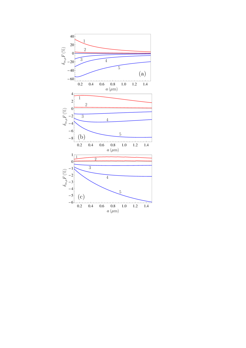
Figure 1: The relative differences of the Casimir force for real and pristine graphene between (a) a Au sphere and a graphene sheet, (b) a Au sphere and a graphene-coated SiO₂ plate and (c) a Au sphere and a graphene-coated Si plate are shown as functions of separation at $T=300\,$K. The lines 1, 2, 3, 4, and 5 correspond to the following five combinations of values of $m$ and $\mu$: $m=0,\>\mu=0.5\,$eV; $m=0,\>\mu=0.1\,$eV; $mc^{2}=0.1\,\mbox{eV},\>\mu=0$; $mc^{2}=0.15\,\mbox{eV},\>\mu=0$; and $mc^{2}=0.2\,\mbox{eV},\>\mu=0$, respectively.

Numerical computations have been performed at $T=300\,$K by using Eqs. (28)–(30), (12) and (14). The computational results in percents as functions of separation are shown in Fig. 1(a) by the five lines 1, 2, 3, 4, and 5 corresponding, respectively, to the following five combinations of values of $m$ and $\mu$: $m=0,\>\mu=0.5\,$eV; $m=0,\>\mu=0.1\,$eV; $mc^{2}=0.1\,\mbox{eV},\>\mu=0$; $mc^{2}=0.15\,\mbox{eV},\>\mu=0$; and $mc^{2}=0.2\,\mbox{eV},\>\mu=0$. [Note that Figs. 1(b) and 1(c), which refer to the case of graphene deposited on a substrate, are discussed in Sec. IV.] As is seen in Fig. 1(a), the presence of nonzero mass gap and chemical potential acts on the Casimir force in opposite directions. The magnitude of the Casimir force decreases with increasing $m$, while it increases with increasing $\mu$. This result finds a simple physical explanation. An increase of the chemical potential essentially increases graphene’s conductivity, so that one should expect the force to grow. On the other hand, by increasing the mass gap one is lowering the mobility, which in turn lowers the conductivity and brings the force down. The relative impact of both parameters decreases with increasing separation distance between the sphere and the graphene sheet.

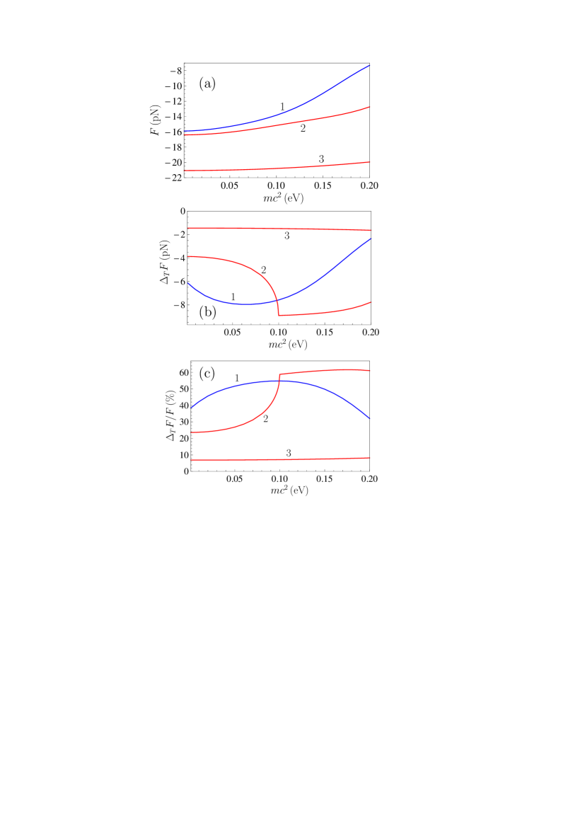
Figure 2: (a) The Casimir force, (b) its thermal correction and (c) the fractional weight of the thermal correction in the Casimir force for a Au sphere interacting with a graphene sheet for $a=0.1\,\mu$m, $T=300\,$K are shown as functions of the mass-gap parameter. The lines 1, 2, and 3 are for $\mu=0$, 0.1, and 0.5 eV, respectively.

We next consider the dependence of the Casimir force between a Au sphere and a graphene sheet and its thermal correction (16) on the value of the mass gap for different values of the chemical potential. When doing that, the Casimir force $F(a,0)$ is computed using the Lifshitz formula at zero temperature, i.e. Eq. (1) with the replacement (17), together with the expressions for the polarization tensor in Eqs. (21), (22), (24), and (25). The computational results for the Casimir force $F$ are shown for $a=0.1\,\mu$m and $T=300\,$K in Fig. 2(a) as functions of the mass gap for three different values of chemical potential $\mu=0$, 0.1, and 0.5 eV, corresponding to lines 1, 2 and 3, respectively. The computational results for the thermal correction to the Casimir force, $\Delta_{T}F$, and for the fractional weight of the thermal correction in the total force, $\Delta_{T}F/F$, are displayed in Figs. 2(b) and 2(c) for the same values of the parameters as in Fig. 2(a).

As is seen in Fig. 2(a), the magnitude of the Casimir force decreases monotonously with increasing $m$ and increases with an increase of $\mu$ in accordance with Fig. 1(a). The values of $F$ in Fig. 2(a) at $m=0$ are in agreement with the computational results of Ref. 66 , where the enhanced thermal Casimir force for nonzero $\mu$ was found. The dependence of the thermal correction to the Casimir force on $m$ in Figs. 2(b) and 2(c) is nonmonotonous (this effect was already noted in Ref. 53 for the case $\mu=0$). The characteristic discontinuity displayed by the derivative of the $\mu=0.1\,$eV curves in Figs. 2(b) and 2(c) for $mc^{2}=0.1\,$eV is explained by the fact that for $\mu=0.1\,$eV the contributions $\Pi_{00}^{(1)}$ and $\Pi^{(1)}$ to the polarization tensor at $T=0$ both turn into zero for $mc^{2}\geq 0.1\,$eV (see Sec. II). Note that for free-standing graphene values of $mc^{2}$ exceeding 0.1 eV are somewhat unrealistic. This region is shown in Figs. 2(b) and 2(c) only for comparison purposes with the case of graphene deposited on a substrate (see Sec. IV). On the whole, under the condition $mc^{2}<\mu$ the thermal effect decreases in magnitude with increasing chemical potential, and its relative role in the Casimir force drops down.

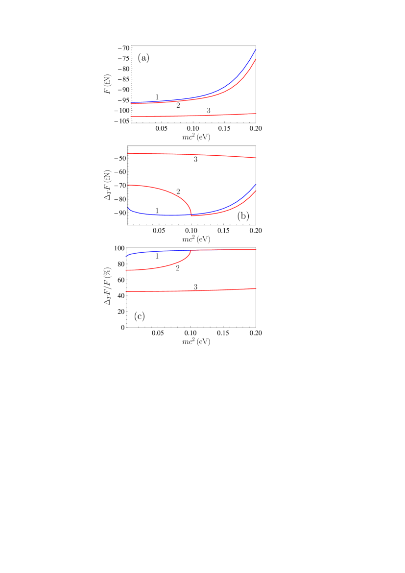
Figure 3: (a) The Casimir force, (b) its thermal correction and (c) the fractional weight of the thermal correction in the Casimir force for a Au sphere interacting with a graphene sheet for $a=1\,\mu$m, $T=300\,$K are shown as functions of the mass-gap parameter. The lines 1, 2, and 3 are for $\mu=0$, 0.1, and 0.5 eV, respectively.

For comparison purposes, the $300\,$K thermal Casimir force between a Au sphere and a free-standing graphene sheet [Fig. 3(a)], its thermal correction [Fig. 3(b)], and the fractional weight of the thermal correction in the total thermal force [Fig. 3(c)] are shown as functions of the mass gap for the larger separation $a=1\,\mu$m for three different values of the chemical potential $\mu=0$, 0.1, and 0.5 eV corresponding, respectively, to lines 1, 2 and 3 in the figures. As it can be seen by a comparison of Figs. 2 and 3, both the Casimir force and its thermal correction have a similar qualitative behavior for the two different separations. Although the magnitudes of the thermal correction at $a=1\,\mu$m are smaller than those found for $a=0.1\,\mu$m [compare Figs. 3(b) and 2(b)], they represent larger fractions of the total force at $a=1\,\mu$m [see Figs. 3(c) and 2(c)]. As is seen in Fig. 3(c), for a sufficiently large mass gap a chemical potential not exceeding 0.1 eV makes almost no impact on the fractional weight of the thermal correction in the total Casimir force.

IV Suppressed impact of the mass gap and chemical
potential for graphene-coated dielectric substrates

Here, we consider the Casimir force and its thermal correction for a Au-coated sphere of $R=150\,\mu$m radius interacting with a real graphene sheet deposited on a dielectric plate. Numerical computations were performed at $T=300\,$K by using the Lifshitz formula (28) for plates made of SiO₂ (vitreous silica) and high-resistivity Si. The reflection coefficients (3) are expressed in terms of dimensionless variables (27) as

$$R_{\rm TM}^{(n)}(i\zeta_{l},y)=\frac{\varepsilon_{l}^{(n)}y(y^{2}-\zeta_{l}^{2})+\sqrt{y^{2}+(\varepsilon_{l}^{(n)}-1)\zeta_{l}^{2}}\left[y\tilde{\Pi}_{00,l}-(y^{2}-\zeta_{l}^{2})\right]}{\varepsilon_{l}^{(n)}y(y^{2}-\zeta_{l}^{2})+\sqrt{y^{2}+(\varepsilon_{l}^{(n)}-1)\zeta_{l}^{2}}\left[y\tilde{\Pi}_{00,l}+(y^{2}-\zeta_{l}^{2})\right]},$$

$$R_{\rm TE}^{(n)}(i\zeta_{l},y)=\frac{(y^{2}-\zeta_{l}^{2})[y-\sqrt{y^{2}+(\varepsilon_{l}^{(n)}-1)\zeta_{l}^{2}}]-\tilde{\Pi}_{l}}{(y^{2}-\zeta_{l}^{2})[y+\sqrt{y^{2}+(\varepsilon_{l}^{(n)}-1)\zeta_{l}^{2}}]+\tilde{\Pi}_{l}}.$$ (33)

We begin with the case of a SiO₂ substrate.

IV.1 Silica plate

The dielectric permittivity of SiO₂ along the imaginary frequency axis, $\varepsilon_{l}^{(2)}\equiv\varepsilon^{(2)}(i\xi_{l})$, can be described very accurately by a simple analytic formula 25 ; 87 ; 87a . The four numerical coefficients involved in this formula have been determined from a fit to the tabulated optical data of SiO₂ 74 . The resulting static dielectric permittivity of SiO₂ is $\varepsilon_{0}^{(2)}=3.81$. Numerical computations of the Casimir force, $F$, and its thermal correction, $\Delta_{T}F$, have been performed at $T=300\,$K using Eqs. (28), (29), (33) together with the expressions for the polarization tensor of graphene presented in Sec. II for both nonzero and zero temperature.

First, we calculate the relative difference $\delta_{m,\mu}F$ among the Casimir forces between a Au sphere and a SiO₂ plate coated either with real graphene characterized by nonzero $m$ and $\mu$ , or with pristine graphene for which $mc^{2}=\mu=0$ [see Eq. (32)]. The computational results for $\delta_{m,\mu}F$ in percents are presented in Fig. 1(b) as functions of separation by the five lines 1, 2, 3, 4, and 5 corresponding to the following combinations of parameters: $m=0,\>\mu=0.5\,$eV; $m=0,\>\mu=0.1\,$eV; $mc^{2}=0.1\,\mbox{eV},\>\mu=0$; $mc^{2}=0.15\,\mbox{eV},\>\mu=0$; and $mc^{2}=0.2\,\mbox{eV},\>\mu=0$, respectively. As is seen in Fig. 1(b), for the graphene-coated substrate the presence of a nonzero mass gap and chemical potential has an opposite effect on the magnitude of the Casimir force similar to the case of a free-standing graphene sheet [see Fig. 1(a)]. The striking difference between the two cases is, however, that for a graphene-coated substrate the impact of nonzero $m$ and $\mu$ is up to an order of magnitude smaller than for a free-standing graphene sheet. This is explained by the fact that the substrate material provides the dominant contribution to the reflection coefficient of the graphene-coated substrate (see a discussion in the next paragraph for more details). It is notable also that for the largest mass considered ($mc^{2}=0.2\,$eV) the magnitude of $\delta_{m,\mu}F$ increases with increasing separation, while this phenomenon is not observed for free-standing graphene with any mass.

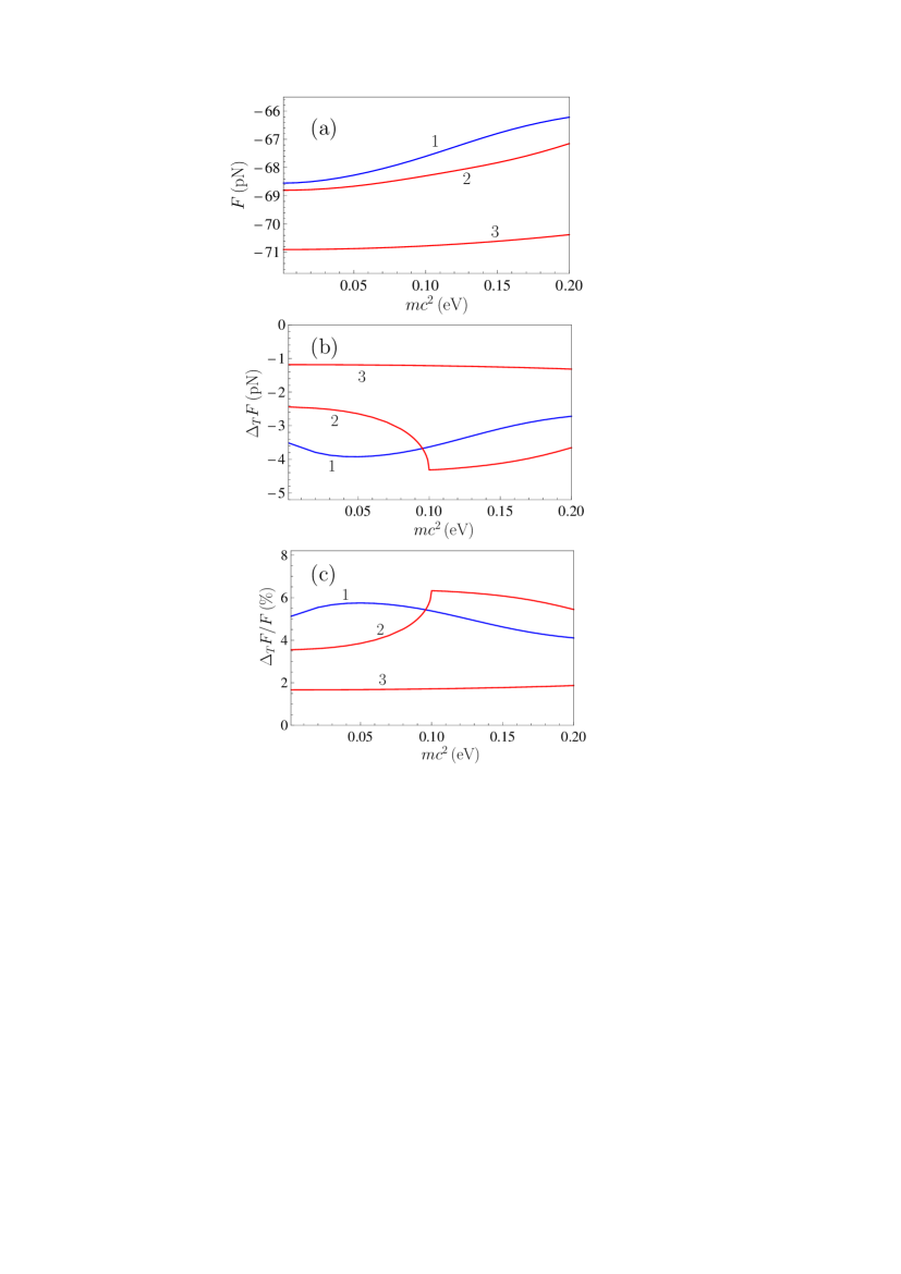
Figure 4: (a) The Casimir force, (b) its thermal correction and (c) the fractional weight of the thermal correction in the Casimir force for a Au sphere interacting with a graphene-coated SiO₂ plate for $a=0.1\,\mu$m, $T=300\,$K are shown as functions of the mass-gap parameter. The lines 1, 2, and 3 are for $\mu=0$, 0.1, and 0.5 eV, respectively.

Next, we present the computational results for the Casimir force between a Au sphere and a graphene-coated SiO₂ plate for $T=300\,$K, $a=0.1\,\mu$m [Fig. 4(a)], its thermal correction [Fig. 4(b)], and the fractional weight of the thermal correction in the Casimir force [Fig. 4(c)] as functions of the mass gap for $\mu=0$, 0.1, and 0.5 eV (lines 1, 2, and 3, respectively). As is seen from the comparison of Figs. 2(a)–2(c) and 4(a)–4(c), the Casimir force, its thermal correction, and the fractional weight of the thermal correction in the force have the same qualitative behavior in the cases of a free-standing graphene and for a graphene-coated SiO₂ substrate. One should note, however, that for a graphene-coated SiO₂ plate the magnitude of the Casimir force is several times larger than for a free-standing graphene [see Figs. 2(a) and 4(a)]. Physically this is explained by the fact that for a graphene-coated substrate the reflection coefficient is much larger than for a free-standing graphene sheet. Specifically, for a free-standing graphene the reflection coefficient is proportional to the fine structure constant. Upon including a substrate, the overall reflection coefficient of the substrate and graphene system is dominated by the large contribution from the substrate material. The latter depends on its dielectric permittivity and corresponds to the zeroth order term in an expansion in powers of the fine structure constant. The magnitude of the thermal correction for a graphene-coated substrate is somewhat smaller and its fractional weight in the total Casimir force is much smaller than for a free-standing graphene sheet. This is seen from the comparison of Fig. 2(b) with Fig. 4(b) and Fig. 2(c) with Fig. 4(c), respectively. One can say that a substrate acts on the zero-temperature force and on the thermal correction to it in opposite directions.

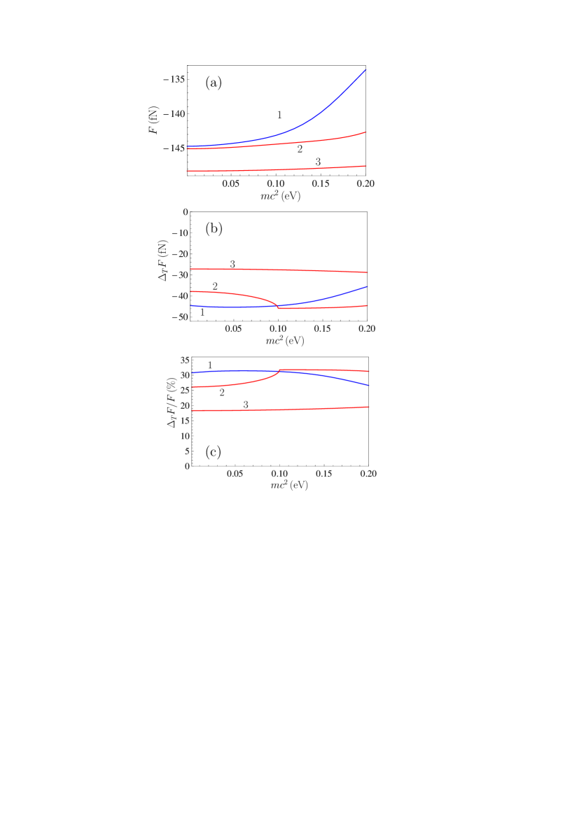
Figure 5: (a) The Casimir force, (b) its thermal correction and (c) the fractional weight of the thermal correction in the Casimir force for a Au sphere interacting with a graphene-coated SiO₂ plate for $a=1\,\mu$m, $T=300\,$K are shown as functions of the mass-gap parameter. The lines 1, 2, and 3 are for $\mu=0$, 0.1, and 0.5 eV, respectively.

Similar to Fig. 4, in Fig. 5 the computational results for $F$, $\Delta_{T}F$ and $\Delta_{T}F/F$ in the case of a graphene-coated SiO₂ plate are presented at $T=300\,$K, but at the larger sphere-plate separation $a=1\,\mu$m. All notations in Fig. 5 are the same as in Fig. 4. As is seen in Fig. 5, the qualitative features of the dependence of all considered quantities on the mass-gap parameter do not change. The magnitude of the Casimir force in Fig. 5(a) is larger and the magnitude of its thermal correction in Fig. 5(b) is smaller than in Figs. 3(a) and 3(b) plotted at the same separation for a free-standing graphene sheet. The fractional weight of the thermal correction in the total force in Fig. 5(c) is up to a factor of 3 smaller than in Fig. 3(c). These results remain valid for any considered value of the chemical potential and mass-gap parameter.

IV.2 Silicon plate

The dielectric permittivity of high-resistivity Si along the imaginary frequency axis $\varepsilon_{l}^{(3)}\equiv\varepsilon^{(3)}(i\xi_{l})$ was obtained from the optical data for its complex index of refraction 74 . Unlike SiO₂, Si possesses a rather large static dielectric permittivity $\varepsilon_{0}^{(3)}=11.66$, and this influences both the Casimir force and its thermal correction. All computations are performed using the same equations as in Sec. IVA.

Specifically, the relative deviations of the Casimir force between a Au sphere and a Si plate coated with either real or pristine graphene as functions of separation are shown in Fig. 1(c) by the five lines for the same pairs ($mc^{2},\,\mu$) for real graphene as in Figs. 1(a) and 1(b). It is again seen that nonzero $m$ and $\mu$ influence the Casimir force in opposite directions. This impact, however, is further decreased as compared to the case of SiO₂ plate.

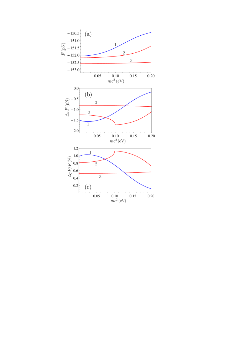
Figure 6: (a) The Casimir force, (b) its thermal correction and (c) the fractional weight of the thermal correction in the Casimir force for a Au sphere interacting with a graphene-coated Si plate for $a=0.1\,\mu$m, $T=300\,$K are shown as functions of the mass-gap parameter. The lines 1, 2, and 3 are for $\mu=0$, 0.1, and 0.5 eV, respectively.

In Figs. 6(a)–6(c) the computational results for the Casimir force between a Au sphere and a graphene-coated Si plate, for its thermal correction and for the fractional weight of the thermal correction in the force are presented for $a=0.1\,\mu$m, $T=300\,$K as functions of the mass gap by the lines 1, 2, and 3 plotted for $\mu=0$, 0.1, and 0.5 eV, respectively. As is seen in Fig. 6(a), the magnitudes of the Casimir force are much larger than for the case of the SiO₂ plate shown in Fig. 4(a), as a result of the larger value $\varepsilon_{0}^{(3)}$ of the static permittivity of Si as compared to $\varepsilon_{0}^{(2)}$ of SiO₂. From Figs. 6(b) and 6(c) it follows, however, that both the thermal correction and its fractional weight in the total force are smaller than for a SiO₂ plate. Hence, for substrates with larger $\varepsilon_{0}$ the impact of graphene coating with nonzero $m$ and $\mu$ becomes smaller. This effect was reported in Ref. 60 for dielectric plates coated with pristine graphene.

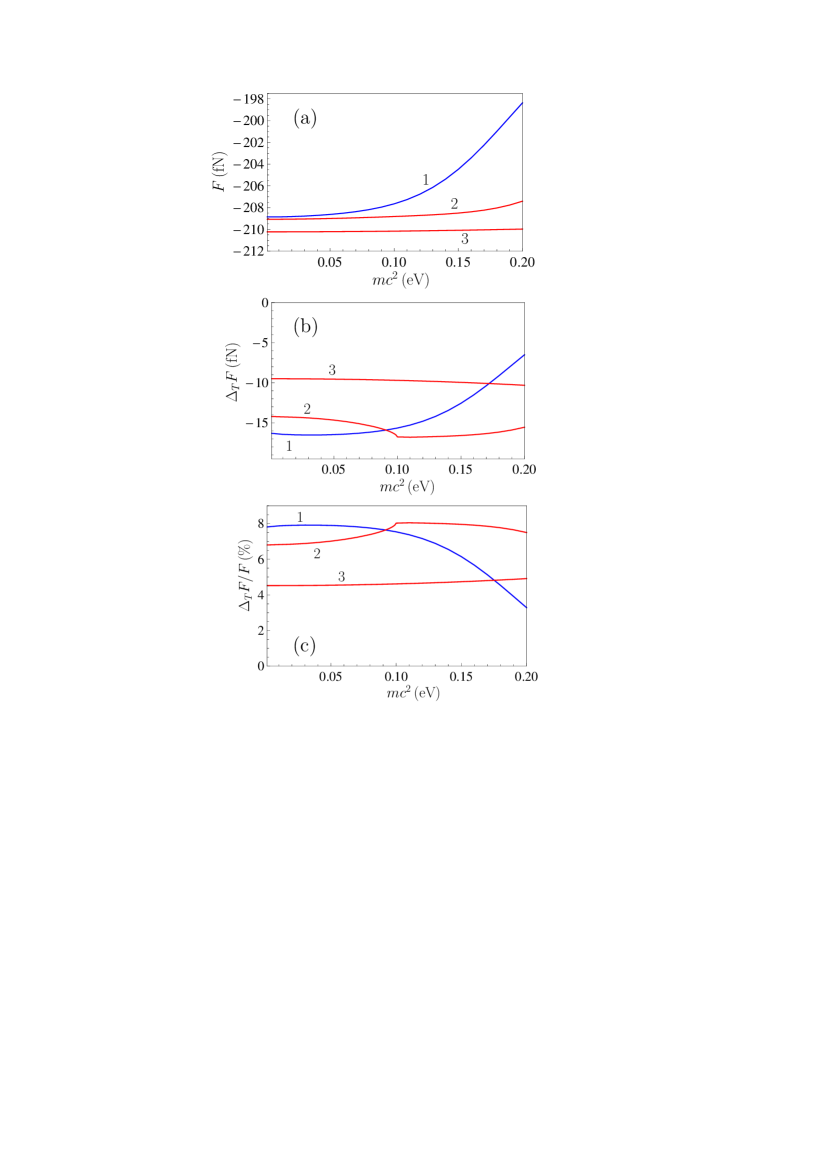
Figure 7: (a) The Casimir force, (b) its thermal correction and (c) the fractional weight of the thermal correction in the Casimir force for a Au sphere interacting with a graphene-coated Si plate for $a=1\,\mu$m, $T=300\,$K are shown as functions of the mass-gap parameter. The lines 1, 2, and 3 are for $\mu=0$, 0.1, and 0.5 eV, respectively.

The analogous computational results for $F$, $\Delta_{T}F$ and $\Delta_{T}F/F$ for the larger separation $a=1\,\mu$m between a Au sphere and a graphene-coated Si plate are shown in Figs. 7(a)–7(c). Notations are the same as in Fig. 6. From Fig. 7(a) one can see that the magnitudes of the Casimir force are much larger than those shown in Fig. 5(a), which refer to the case of a graphene-coated SiO₂ plate. The magnitudes of the thermal correction in Fig. 7(b) and its fractional weight in the total force in Fig. 7(c) are smaller, compared to the case of a SiO₂ substrate at the same separation distance [see Figs. 5(b) and 5(c)].

V Role of nonzero mass gap and chemical potential in differential measurements of the thermal effect for graphene

It has long been known that differential measurements allow to achieve a very high precision and reliability. In Casimir physics they were used to measure the optically modulated Casimir force between a Au sphere and a Si plate illuminated with laser pulses 88 and in the so-called Casimir-less experiments searching for Yukawa-type corrections to Newton’s gravitational law 89 ; 90 . Recently it was found that differential measurement schemes allow for a huge amplification of the difference among the theoretical predictions of the Lifshitz theory using either the Drude or the plasma model in the extrapolation of optical data down to zero frequency 91 ; 92 ; 93 . Using one of these differential schemes, in which the difference among the alternative theoretical predictions could be made as large as by a factor of 1000, the experiment of Ref. 82 confirmed the plasma model approach to the Casimir force between metallic test bodies and undeniably excluded the Drude model. This result provided further support to several previous measurements in favor of the plasma model 75 ; 76 ; 77 ; 78 ; 79 ; 80 ; 81 , in which, however, the predicted difference between the two approaches did not exceed a few percent. Very recently, a universal differential measurement has been proposed which allows for a clear discrimination between different theoretical approaches to the Casimir force not only for metallic, but also for dielectric test bodies 94 .

In this section, we consider the role of nonzero mass gap and chemical potential in the differential setup aiming at the observation of the giant thermal effect in graphene systems, proposed by us in Ref. 67 . In that work it was shown that the thermal effect can be observed, using a feasible adaptation of a currently available experimental setup, by measuring the difference among the Casimir forces between a Au-coated sphere and the two halves of a Si plate, one of which is coated and the other is uncoated with a graphene sheet 67 . Since in Ref. 67 the parameters for pristine graphene have been used in the computations, it is now important to check whether the encouraging conclusions reached there concerning the feasibility of this experiment remain valid for real graphene samples which posses nonzero mass gap and chemical potential.

We recall that in Ref. 67 we proposed to measure the differential force

$$F_{\rm diff}(a,T)=F_{\rm Si}(a,T)-F(a,T),$$ (34)

where $F(a,T)$ is the Casimir force between a Au-coated sphere and a graphene-coated Si plate expressed by Eqs. (28), (29), and (33), and $F_{\rm Si}(a,T)$ is the Casimir force between a Au sphere and uncoated Si plate. The latter force is also expressed by the Lifshitz formula (28), in which the reflection coefficients (29) remain unchanged. The reflection coefficients $R_{\alpha}^{(3)}$ are replaced with coefficients of the uncovered Si plate having a form analogous to Eq. (29) in which, however, the dielectric permittivity $\varepsilon_{l}^{(1)}$ of Au is replaced by the permittivity $\varepsilon_{l}^{(3)}$ of Si.

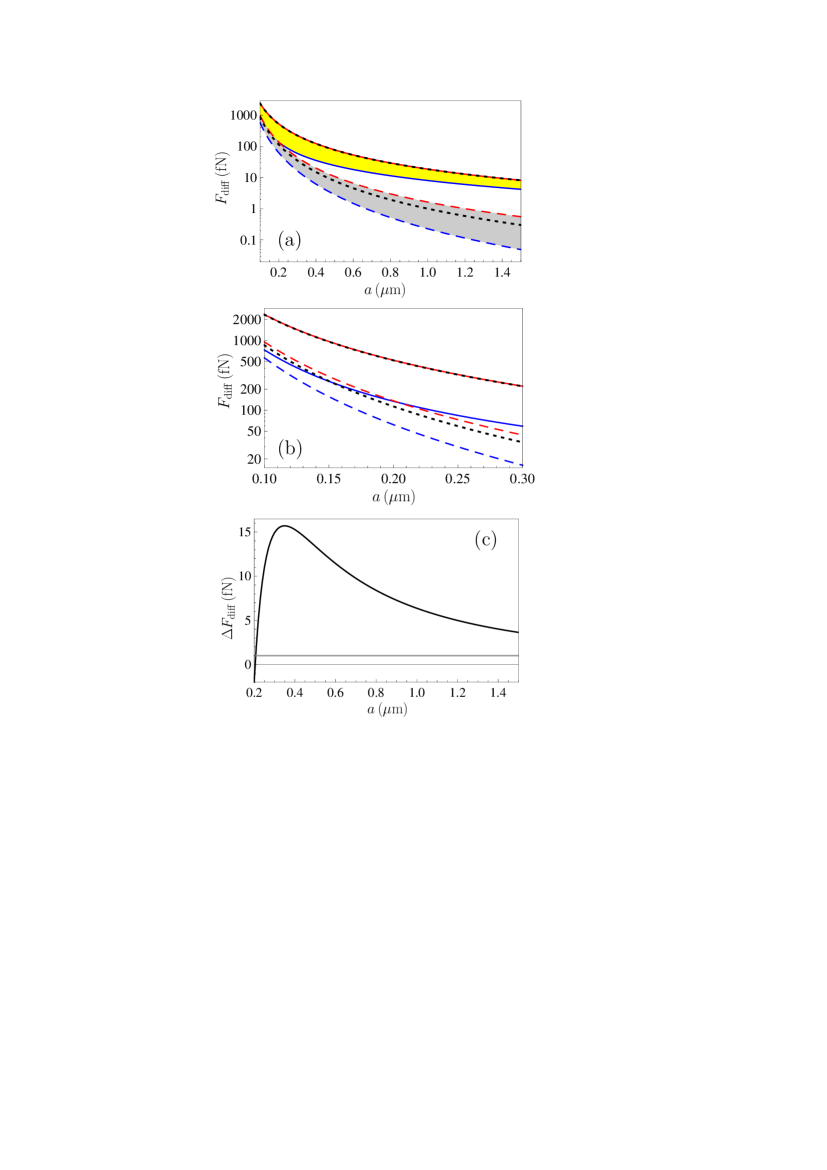
Figure 8: (a) The difference among the Casimir forces between a Au sphere and uncoated and graphene-coated Si plate is shown as a function of separation. The top and bottom solid lines are plotted at $T=300\,$K for $mc^{2}=0,\,\mu=0.02\,$eV and for $mc^{2}=0.2\,\mbox{eV},\,\mu=0$, respectively. The top and bottom dashed lines are plotted at $T=0\,$K for the same respective pairs of values for $mc^{2}$ and $\mu$. The top and bottom dotted lines are plotted for the pristine graphene at $T=300\,$K and $T=0\,$K, respectively. (b) The region of short separations from (a) is shown on an enlarged scale. (c) The difference between the bottom solid and top dashed lines in (a) is shown by the top solid line in comparison with the experimental error (the horizontal line) as a function of separation.

Using these formulas we have performed numerical computations of $F_{\rm diff}$ as a function of separation. The computational results for $T=300\,$K are shown in Fig. 8(a) by the top and bottom solid lines plotted for $mc^{2}=0$, $\mu=0.02\,$eV and $mc^{2}=0.2\,$eV, $\mu=0$, respectively. The top and bottom dashed lines in this figure show the computational results for $F_{\rm diff}$ at $T=0$ for the same two combinations of values ($m,\,\mu$). We remind that $\mu=0.02\,$eV represents the value of the chemical potential for the graphene samples used in the experiment 35 , which measured the gradient of the Casimir force between a Au-coated sphere and graphene-coated substrate, whereas $mc^{2}=0.2\,$ represents the estimated upper bound on the value of $mc^{2}$ for graphene-coated substrates. Therefore, one can confidently conclude that for realistic samples the thermal correction to the differential force (34),

$$\Delta_{T}F_{\rm diff}(a,T)=F_{\rm diff}(a,T)-F_{\rm diff}(a,0),$$ (35)

belongs to the band defined by the difference between the two bands bounded, respectively, by the two pairs of solid and dashed lines in Fig. 8(a). The upper bound on the band for $\Delta_{T}F_{\rm diff}$ is therefore equal to the difference among the top solid and bottom dashed lines in Fig. 8(a), while its lower bound is equal to the difference among the bottom solid and top dashed lines of that figure.

The top and bottom dotted lines in Fig. 8(a) were computed supposing that half of the Si plate is coated not with a real, but rather with a pristine graphene for $T=300\,$K and $T=0$, respectively. The difference among these lines was used as an estimate of $\Delta_{T}F_{\rm diff}$ in Ref. 67 . As is seen in Fig. 8(a), the top solid line ($T=300\,$K, $mc^{2}=0$, $\mu=0.02\,$eV) and the top dotted line ($T=300\,$K, pristine graphene) are almost coinciding. This indicates that the chemical potential $\mu=0.02\,$eV does not influence the value of the Casimir force. For a better visualization, in Fig. 8(b) the region of short separations is shown on an enlarged scale.

Now we are in a position to determine the feasibility of the proposed experiment on measuring the giant thermal effect in graphene systems with full account of the nonzero mass gap and chemical potential of real samples. For this purpose, in Fig. 8(c) we plot the minimum value of the thermal correction in $F_{\rm diff}$,

$$\Delta F_{\rm diff}(a,T)=\min\Delta_{T}F_{\rm diff}(a,T),$$ (36)

which is equal to the difference between the bottom solid and top dashed lines in Fig. 8(a). The horizontal line in Fig. 8(c) indicates the magnitude of the experimental error of 1 fN achieved in a differential measurement of the Casimir force that has been performed already 82 . As is seen in Fig. 8(c), even taking into account the mass gap and chemical potential, the minimum possible value of the thermal correction $\Delta F_{\rm diff}$ far exceeds the experimental error over the wide separation region from 220 nm to $1.5\,\mu$m. Thus, the proposed experiment allows for a reliable observation of the giant thermal effect for real graphene samples.

VI Conclusions and discussion

In the foregoing we have investigated the impact of nonzero mass gap and chemical potential on the Casimir force and its thermal correction for graphene systems. The experimentally relevant configurations of a Au-coated sphere interacting with either a free-standing graphene sheet or graphene-coated dielectric substrates made of different materials have been the focus of our attention. It was found that the mass gap and chemical potential produce pronounced effects on both the Casimir force and its thermal correction, indicating that both quantities should be taken into account in investigations of fluctuation-induced phenomena in graphene and other 2D-materials, as well as in prospective applications of these phenomena to nano- and micromechanical systems.

According to our results, which were derived in the framework of the rigorous QED approach based on the exact finite-temperature polarization tensor of graphene, the mass gap and chemical potential act in opposite directions on the magnitude of the Casimir force. Specifically, it was shown that with increasing $m$ and fixed $\mu$ the magnitude of the Casimir force decreases, whereas it increases with increasing $\mu$ and fixed $m$. This behavior, which is observed both for a free-standing graphene sheet and for graphene deposited on a substrate, leads to a partial compensation of both effects when the Casimir force is worked out taking into account the simultaneous influence of nonzero $m$ and $\mu$. Although, as discussed in Secs. III and IV, the above results are quite expected on physical grounds, a precise quantitative evaluation requires the use of the formalism presented in this work.

Another important property demonstrated in this paper is that the impacts of nonzero mass gap and chemical potential on the Casimir force for graphene-coated plates are both much smaller than for a free-standing graphene sheet. Since most applications use graphene-coated substrates, our results suggest that the possibility of controlling the Casimir force by means of the chemical potential is somewhat problematic.

Our computational results show that the magnitude of the Casimir force for graphene-coated substrates is much larger than for a free-standing graphene, but the thermal correction and its fractional weight in the total force are smaller. The computations made for SiO₂ and Si plates demonstrate that the influence of the graphene coating on the Casimir force and its thermal correction decreases when the substrate has a higher static dielectric permittivity. Our investigation of the dependence of the thermal correction on the mass gap for different values of the chemical potential revealed the existence of a discontinuity of the derivative of the Casimir force with respect to $mc^{2}$ for $mc^{2}=\mu$. The origin of this discontinuity resides in the fact that for values of the chemical potential such that $\mu\leq mc^{2}$ the zero-temperature polarization tensor of graphene is independent of $\mu$.

Finally, we have determined the role of nonzero $m$ and $\mu$ in a differential experiment recently proposed by us 67 to observe the giant thermal effect in the Casimir force at short separations. For this purpose, the differential Casimir force between a Au sphere and the two halves of a Si plate, one uncoated and the other coated with graphene, was computed as a function of separation, taking into account the influence of $m$ and $\mu$. We estimated the minimum value of the thermal correction to the Casimir force as a function of separation with the same value of the chemical potential as for graphene samples in a recent experiment probing the Casimir force between a Au sphere and a graphene-coated substrate 35 . In this computation we conservatively used the maximum possible value for the mass-gap parameter. Comparison with the force sensitivity of state-of-the-art differential Casimir setups confirms the feasibility of the proposed experiment with account of $m$ and $\mu$.

The formalism for the calculation of the thermal Casimir force in graphene systems accounting for nonzero $m$ and $\mu$, presented in this work, opens many novel opportunities in both fundamental and applied research. For example, it may allow for a determination of the mass gap of a graphene sheet by fitting the experimental data for the giant thermal effect to the theoretical results obtained with different values of $m$. A direct observation of the giant thermal effect in graphene, combined with first-principle computations, might open novel opportunities for the modification and control of the Casimir force in graphene-based micromechanical systems.

References

- (1) P. J. F. Harris, Carbon Nanotubes and Related Structures: New Materials for the Twenty-First Century (Cambridge University Press, New York, 1999).
- (2) Physics of Graphene, ed. H. Aoki and M. S. Dresselhaus (Springer, Cham, 2014).
- (3) M. I. Katsnelson, Graphene: Carbon in Two Dimensions (Cambridge University Press, Cambridge, 2012).
- (4) M. O. Goerbig, Rev. Mod. Phys. 83, 1193 (2011).
- (5) M. I. Katsnelson, K. S. Novoselov, and A. K. Geim, Nature Phys. 2, 620 (2006).
- (6) D. Allor, T. D. Cohen, and D. A. McGady, Phys. Rev. D 78, 096009 (2008).
- (7) C. G. Beneventano, P. Giacconi, E. M. Santangelo, and R. Soldati, J. Phys. A 42, 275401 (2009).
- (8) G. L. Klimchitskaya and V. M. Mostepanenko, Phys. Rev. D 87, 125011 (2013).
- (9) I. Akal, R. Egger, C. Müller, and S. Villarba-Chávez, Phys. Rev. D 93, 116006 (2016).
- (10) A. W. W. Ludwig, M. P. A. Fisher, R. Shankar, and G. Grinstein, Phys. Rev. B 50, 7526 (1994).
- (11) T. Ando, Y. Zheng, and H. Suzuura, J. Phys. Soc. Jpn. 71, 1318 (2002).
- (12) L. A. Falkovsky and A. A. Varlamov, Eur. Phys. J. B 56, 281 (2007).
- (13) T. Stauber, N. M. R. Peres, and A. K. Geim, Phys. Rev. B 78, 085432 (2008).
- (14) M. Lewkowicz and B. Rosenstein, Phys. Rev. Lett. 102, 106802 (2009).
- (15) T. Stauber, J. Phys.: Condens. Matter 26, 123201 (2014).
- (16) M. Merano, Phys. Rev. A 93, 013832 (2016).
- (17) G. L. Klimchitskaya and V. M. Mostepanenko, Phys. Rev. B 93, 245419 (2016).
- (18) G. L. Klimchitskaya and V. M. Mostepanenko, Phys. Rev. B 94, 195405 (2016).
- (19) L. A. Falkovsky and S. S. Pershoguba, Phys. Rev. B 76, 153410 (2007).
- (20) R. R. Nair, P. Blake, A. N. Grigorenko, K. S. Novoselov, T. J. Booth, T. Stauber, N. M. R. Peres, and A. K. Geim, Science 320, 1308 (2008).
- (21) F. H. L. Koppens, D. E. Chang, and F. J. García de Abajo, Nano Lett. 11, 3370 (2011).
- (22) M. Bordag, G. L. Klimchitskaya, V. M. Mostepanenko, and V. M. Petrov, Phys. Rev. D 91, 045037 (2015); 93, 089907(E) (2016).
- (23) G. L. Klimchitskaya, C. C. Korikov, and V. M. Petrov, Phys. Rev. B 92, 125419 (2015); 93, 159906(E) (2016).
- (24) G. L. Klimchitskaya and V. M. Mostepanenko, Phys. Rev. A 93, 052106 (2016).
- (25) G. L. Klimchitskaya and V. M. Mostepanenko, Phys. Rev. B 95, 035425 (2017).
- (26) M. Bordag, G. L. Klimchitskaya, U. Mohideen, and V. M. Mostepanenko, Advances in the Casimir Effect (Oxford University Press, Oxford, 2015).
- (27) E. M. Lifshitz and L. P. Pitaevskii, Statistical Physics, Part II (Pergamon, Oxford, 1980).
- (28) G. Barton, J. Phys. A: Math. Gen. 38, 2997 (2005).
- (29) M. Bordag, J. Phys. A: Math. Gen. 39, 6173 (2006).
- (30) M. Bordag, B. Geyer, G. L. Klimchitskaya, and V. M. Mostepanenko, Phys. Rev. B 74, 205431 (2006).
- (31) M. Bordag, Phys. Rev. D 75, 065003 (2007).
- (32) E. V. Blagov, G. L. Klimchitskaya, and V. M. Mostepanenko, Phys. Rev. B 75, 235413 (2007).
- (33) M. Bordag and N. Khusnutdinov, Phys. Rev. D 77, 085026 (2008).
- (34) N. R. Khusnutdinov, Phys. Rev. B 83, 115454 (2011).
- (35) G. L. Klimchitskaya and V. M. Mostepanenko, Phys. Rev. B 91, 045412 (2015).
- (36) A. A. Banishev, H. Wen, J. Xu, R. K. Kawakami, G. L. Klimchitskaya, V. M. Mostepanenko, and U. Mohideen, Phys. Rev. B 87, 205433 (2013).
- (37) A. H. Castro Neto, F. Guinea, N. M. R. Peres, K. S. Novoselov, and A. K. Geim, Rev. Mod. Phys. 81, 109 (2009).
- (38) N. M. R. Peres, Rev. Mod. Phys. 82, 2673 (2010).
- (39) J. F. Dobson, A. White, and A. Rubio, Phys. Rev. Lett. 96, 073201 (2006).
- (40) G. Gómez-Santos, Phys. Rev. B 80, 245424 (2009).
- (41) D. Drosdoff and L. M. Woods, Phys. Rev. B 82, 155459 (2010).
- (42) D. Drosdoff and L. M. Woods, Phys. Rev. A 84, 062501 (2011).
- (43) Bo E. Sernelius, Europhys. Lett. 95, 57003 (2011).
- (44) T. E. Judd, R. G. Scott, A. M. Martin, B. Kaczmarek, and T. M. Fromhold, New J. Phys. 13, 083020 (2011).
- (45) J. Sarabadani, A. Naji, R. Asgari, and R. Podgornik, Phys. Rev. B 84, 155407 (2011); Phys. Rev. B 87, 239905(E) (2013).
- (46) D. Drosdoff, A. D. Phan, L. M. Woods, I. V. Bondarev, and J. F. Dobson, Eur. Phys. J. B 85, 365 (2012).
- (47) Bo E. Sernelius, Phys. Rev. B 85, 195427 (2012).
- (48) A. D. Phan, L. M. Woods, D. Drosdoff, I. V. Bondarev, and N. A. Viet, Appl. Phys. Lett. 101, 113118 (2012).
- (49) A. D. Phan, N. A. Viet, N. A. Poklonski, L. M. Woods, and C. H. Le, Phys. Rev. B 86, 155419 (2012).
- (50) W.-K. Tse and A. H. Macdonald, Phys. Rev. Lett. 109, 236806 (2012).
- (51) T. Cysne, W. J. M. Kort-Kamp, D. Oliver, F. A. Pinheiro, F. S. S. Rosa, and C. Farina, Phys. Rev. A 90, 052511 (2014).
- (52) V. B. Svetovoy and G. Palasantzas, Phys. Rev. Applied 2, 034006 (2014).
- (53) N. Knusnutdinov, R. Kashapov, and L. M. Woods, Phys. Rev. A 94, 012513 (2016).
- (54) T. P. Cysne, T. G. Rappoport, A. Ferreira, J. M. Viana Parente Lopes, and N. R. M. Peres, Phys. Rev. B 94, 235405 (2016).
- (55) L. M. Woods, D. A. R. Dalvit, A. Tkatchenko, P. Rodrigues-Lopez, A. W. Rodrigues, and R. Podgornik, Rev. Mod. Phys. 88, 045003 (2016).
- (56) A. I. Akhiezer and V. B. Berestetskii, Quantum Electrodynamics (Interscience, New York, 1965).
- (57) S. S. Schweber, An Introduction to Relativistic Quantum Field Theory (Dover, New York, 2005).
- (58) M. Bordag, I. V. Fialkovsky, D. M. Gitman, and D. V. Vassilevich, Phys. Rev. B 80, 245406 (2009).
- (59) I. V. Fialkovsky, V. N. Marachevsky, and D. V. Vassilevich, Phys. Rev. B 84, 035446 (2011).
- (60) M. Bordag, G. L. Klimchitskaya, and V. M. Mostepanenko, Phys. Rev. B 86, 165429 (2012).
- (61) M. Chaichian, G. L. Klimchitskaya, V. M. Mostepanenko, and A. Tureanu, Phys. Rev. A 86, 012515 (2012).
- (62) G. L. Klimchitskaya and V. M. Mostepanenko, Phys. Rev. B 87, 075439 (2013).
- (63) B. Arora, H. Kaur, and B. K. Sahoo, J. Phys. B 47, 155002 (2014).
- (64) K. Kaur, J. Kaur, B. Arora, and B. K. Sahoo, Phys. Rev. B 90, 245405 (2014).
- (65) G. L. Klimchitskaya and V. M. Mostepanenko, Phys. Rev. A 89, 012516 (2014).
- (66) G. L. Klimchitskaya and V. M. Mostepanenko, Phys. Rev. B 89, 035407 (2014).
- (67) G. L. Klimchitskaya and V. M. Mostepanenko, Phys. Rev. A 89, 052512 (2014).
- (68) G. L. Klimchitskaya and V. M. Mostepanenko, Phys. Rev. A 89, 062508 (2014).
- (69) G. L. Klimchitskaya, V. M. Mostepanenko, and Bo E. Sernelius, Phys. Rev. B 89, 125407 (2014).
- (70) G. L. Klimchitskaya, U. Mohideen, and V. M. Mostepanenko, Phys. Rev. B 89, 115419 (2014).
- (71) G. L. Klimchitskaya and V. M. Mostepanenko, Phys. Rev. B 91, 174501 (2015).
- (72) G. L. Klimchitskaya, Int. J. Mod. Phys. A 31, 1641026 (2016).
- (73) V. B. Bezerra, G. L. Klimchitskaya, V. M. Mostepanenko, and C. Romero, Phys. Rev. A 94, 042501 (2016).
- (74) M. Bordag, I. Fialkovskiy, and D. Vassilevich, Phys. Rev. B 93, 075414 (2016); 95, 119905(E) (2017).
- (75) G. Bimonte, G. L. Klimchitskaya, and V. M. Mostepanenko, Phys. Rev. A 96, 012517 (2017).
- (76) C. D. Fosco, F. C. Lombardo, and F. D. Mazzitelli, Phys. Rev. D 84, 105031 (2011).
- (77) G. Bimonte, T. Emig, R. L. Jaffe, and M. Kardar, Europhys. Lett. 97, 50001 (2012).
- (78) G. Bimonte, T. Emig, and M. Kardar, Appl. Phys. Lett. 100, 074110 (2012).
- (79) L. P. Teo, Phys. Rev. D 88, 045019 (2013).
- (80) M. Hartmann, G.-L. Ingold, and P. A. Maia Neto, Phys. Rev. Lett. 119, 043901 (2017).
- (81) G. Bimonte, Europhys. Lett. 118, 20002 (2017).
- (82) A. Schmitt, Dense Matter in Compact Stars: A Pedagogical Introduction (Springer, Berlin, 2010).
- (83) G. L. Klimchitskaya, U. Mohideen, and V. M. Mostepanenko, Rev. Mod. Phys. 81, 1827 (2009).
- (84) Handbook of Optical Constants of Solids, ed. E. D. Palik (Academic, New York, 1985).
- (85) R. S. Decca, E. Fischbach, G. L. Klimchitskaya, D. E. Krause, D. López, and V. M. Mostepanenko, Phys. Rev. D 68, 116003 (2003).
- (86) R. S. Decca, D. López, E. Fischbach, G. L. Klimchitskaya, D. E. Krause, and V. M. Mostepanenko, Ann. Phys. (N.Y.) 318, 37 (2005).
- (87) R. S. Decca, D. López, E. Fischbach, G. L. Klimchitskaya, D. E. Krause, and V. M. Mostepanenko, Phys. Rev. D 75, 077101 (2007).
- (88) R. S. Decca, D. López, E. Fischbach, G. L. Klimchitskaya, D. E. Krause, and V. M. Mostepanenko, Eur. Phys. J. C 51, 963 (2007).
- (89) C.-C. Chang, A. A. Banishev, R. Castillo-Garza, G. L. Klimchitskaya, V. M. Mostepanenko, and U. Mohideen, Phys. Rev. B 85, 165443 (2012).
- (90) A. A. Banishev, G. L. Klimchitskaya, V. M. Mostepanenko, and U. Mohideen, Phys. Rev. Lett. 110, 137401 (2013).
- (91) A. A. Banishev, G. L. Klimchitskaya, V. M. Mostepanenko, and U. Mohideen, Phys. Rev. B 88, 155410 (2013).
- (92) G. Bimonte, D. López, and R. S. Decca, Phys. Rev. B 93, 184434 (2016).
- (93) P. K. Pyatkovskiy, J. Phys.: Condens. Matter 21, 025506 (2009).
- (94) V. P. Gusynin, S. G. Sharapov, and J. P. Carbotte, New J. Phys. 11, 095013 (2009).
- (95) S. A. Jafari, J. Phys.: Condens. Matter 24, 205802 (2012).
- (96) E. M. Hajaj, O. Shtempluk, V. Kochetkov, A. Razin, and Y. E. Yaish, Phys. Rev. B 88, 045128 (2013).
- (97) K. F. Mak, M. Y. Sfeir, Y. Wu, C. H. Lui, J. A. Misewich, and T. F. Heinz, Phys. Rev. Lett. 101, 196405 (2008).
- (98) D. B. Hough and L. R. White, Adv. Coll. Interface Sci. 14, 3 (1980).
- (99) L. Bergström, Adv. Coll. Interface Sci. 70, 125 (1997).
- (100) F. Chen, G. L. Klimchitskaya, V. M. Mostepanenko, and U. Mohideen, Phys. Rev. B 76, 035338 (2007).
- (101) R. S. Decca, D. López, H. B. Chan, E. Fischbach, D. E. Krause, and C. R. Jamell, Phys. Rev. Lett. 94, 240401 (2005).
- (102) Y.-J. Chen, W. K. Tham, D. E. Krause, D. López, E. Fischbach, and R. S. Decca, Phys. Rev. Lett. 116, 221102 (2016).
- (103) G. Bimonte, Phys. Rev. Lett. 112, 240401 (2014).
- (104) G. Bimonte, Phys. Rev. Lett. 113, 240405 (2014).
- (105) G. Bimonte, Phys. Rev. B 91, 205443 (2015).
- (106) G. Bimonte, G. L. Klimchitskaya, and V. M. Mostepanenko, Phys. Rev. A 95, 052508 (2017).