EUROPEAN ORGANIZATION FOR NUCLEAR RESEARCH (CERN)

​​​ CERN-EP-2017-164 LHCb-PAPER-2017-016

Measurement of the shape of the ${{\mathchar 28931\relax}^{0}_{b}}\rightarrow{{\mathchar 28931\relax}^{+}_{c}}{\mu^{-}}{{\overline{\nu}}_{\mu}}$ differential decay rate

The LHCb collaboration

A measurement of the shape of the differential decay rate and the associated Isgur-Wise function for the decay ${{\mathchar 28931\relax}^{0}_{b}}\!\rightarrow{{\mathchar 28931\relax}^{+}_{c}}{\mu^{-}}{{\overline{\nu}}_{\mu}}$ is reported, using data corresponding to $3\mbox{\,fb}^{-1}$ collected with the LHCb detector in proton-proton collisions. The ${{\mathchar 28931\relax}^{+}_{c}}{\mu^{-}}{{\overline{\nu}}_{\mu}}$(+ anything) final states are reconstructed through the detection of a muon and a ${{\mathchar 28931\relax}^{+}_{c}}$ baryon decaying into $p{{K}^{-}}{{\pi}^{+}}$, and the decays ${{\mathchar 28931\relax}^{0}_{b}}\rightarrow{{\mathchar 28931\relax}^{+}_{c}}{{\pi}^{+}}{{\pi}^{-}}{\mu^{-}}{{\overline{\nu}}_{\mu}}$ are used to determine contributions from ${{\mathchar 28931\relax}^{0}_{b}}\rightarrow\mathchar 28931\relax_{c}^{\ast+}{\mu^{-}}{{\overline{\nu}}_{\mu}}$ decays. The measured dependence of the differential decay rate upon the squared four-momentum transfer between the heavy baryons, ${q^{2}}$, is compared with expectations from heavy-quark effective theory and from unquenched lattice QCD predictions.

Published in Phys. Rev. D

© CERN on behalf of the LHCb collaboration, licence CC-BY-4.0.

 

1 Introduction

In the Standard Model (SM) of particle physics, quarks participate in a rich pattern of flavor-changing transitions. The relevant couplings form a complex 3$\times$3 matrix, known as the Cabibbo-Kobayashi-Maskawa (CKM) matrix, characterized by just four independent parameters [1]. A vast body of measurements of individual CKM elements exists, and thus the overall consistency of the SM picture of charged current interactions is highly over-constrained. Decades of experimental work have demonstrated the impressive consistency of experimental data with the CKM paradigm [2, 3]; nonetheless, the motivation to probe the CKM matrix remains strong. Effects of physics beyond the SM may be subtle, thus more precise measurements are necessary to unveil them. Semileptonic decays of heavy-flavored hadrons are commonly used to measure CKM parameters, as they involve only one hadronic current, parameterized in terms of scalar functions known as form factors. The number of form factors needed to describe a particular decay depends upon the spin of the initial- and final-state hadrons [4, 5]. A precise calculation of these form factors has been elusive for many years as it is not possible in perturbative QCD. Heavy-Quark Effective Theory (HQET) provides the framework to systematically include nonperturbative corrections in computations involving hadrons containing heavy quarks. In particular, in the limit of infinite heavy quark mass, all the form factors describing the semileptonic decay of a heavy-flavored hadron are proportional to a universal function, known as the Isgur-Wise (IW) function[6]. Lattice QCD, namely the use of lattice formulations of QCD in large scale numerical simulations, has emerged in recent years as a technique with well defined and systematically improvable uncertainties which can be applied to a wide range of processes and physical quantities[7]. Predictions from the infinite heavy-quark mass limit are useful as a check of several Lattice QCD calculations [8].

The decay ${{\mathchar 28931\relax}^{0}_{b}}\rightarrow{{\mathchar 28931\relax}^{+}_{c}}{\mu^{-}}{{\overline{\nu}}_{\mu}}$ is described by six form factors corresponding to the vector and axial-vector components of the flavor-changing charged current [9]. In HQET, ${{\mathchar 28931\relax}^{0}_{b}}$ decays are particularly simple, as the light ${u}{d}$ quark pair has total spin $j=0$, and thus the chromomagnetic corrections, which are of the order of a few percent for $B$ mesons, are not present [10]. In the static approximation of infinite heavy quark masses, the six form factors characterizing the baryonic semileptonic decay ${{\mathchar 28931\relax}^{0}_{b}}\rightarrow{{\mathchar 28931\relax}^{+}_{c}}{\mu^{-}}{{\overline{\nu}}_{\mu}}$ can be expressed in terms of the elastic heavy-baryon Isgur-Wise function $\xi_{B}(w)$ [11]. The scalar invariant $w\equiv v_{{{\mathchar 28931\relax}^{0}_{b}}}\cdot v_{{{\mathchar 28931\relax}^{+}_{c}}}$ is related to the squared four-momentum transfer between the heavy baryons, ${q^{2}}$, by

$$w=(m_{{{\mathchar 28931\relax}^{0}_{b}}}^{2}+m_{{{\mathchar 28931\relax}^{+}_{c}}}^{2}-q^{2})/(2m_{{{\mathchar 28931\relax}^{0}_{b}}}m_{{{\mathchar 28931\relax}^{+}_{c}}}),$$ (1)

where $v_{{{\mathchar 28931\relax}^{0}_{b}}}$ and $v_{{{\mathchar 28931\relax}^{+}_{c}}}$ are the four-velocities of the ${{\mathchar 28931\relax}^{0}_{b}}$ and ${{\mathchar 28931\relax}^{+}_{c}}$ baryons, respectively, and $m_{{{\mathchar 28931\relax}^{0}_{b}}}$ and $m_{{{\mathchar 28931\relax}^{+}_{c}}}$ are the corresponding invariant masses. Nonperturbative corrections to the static limit can be expressed in terms of an expansion in powers of 1/$m_{c}$ and 1$/m_{b}$, where $m_{c}$ and $m_{b}$ represent the $c$- and $b$-quark masses respectively. It has been shown in Ref. [12] that the 1/$m_{c}$ term can be expressed in terms of $\xi_{B}(w)$ and one dimensionful constant. Moreover, partial cancellations lead to small first-order corrections near $w=1$ [13].

In the static approximation the differential decay width of the ${{\mathchar 28931\relax}^{0}_{b}}\rightarrow{{\mathchar 28931\relax}^{+}_{c}}{\mu^{-}}{{\overline{\nu}}_{\mu}}$ decay is given by

$$\frac{d\Gamma}{dw}=GK(w)\xi^{2}_{B}(w),$$ (2)

where the constant factor $G$ is given by

$$G=\frac{2}{3}\frac{G_{F}^{2}}{(2\pi)^{3}}|V_{cb}|^{2}(m_{{{\mathchar 28931\relax}^{0}_{b}}})^{4}r^{2}~{}~{}\text{with}~{}~{}r=m_{{{\mathchar 28931\relax}^{+}_{c}}}/m_{{{\mathchar 28931\relax}^{0}_{b}}},$$ (3)

where $G_{F}$ represents the Fermi coupling constant [14], $|{V_{{c}{b}}}|$ is the magnitude of the matrix element describing the coupling of the ${c}$ quark to the ${b}$ quark, and the kinematic factor $K(w)$ is given by

$$K(w)=m_{{{\mathchar 28931\relax}^{+}_{c}}}\sqrt{w^{2}-1}\ [3w(1-2rw+r^{2})+2r(w^{2}-1)].$$ (4)

The function $\xi_{B}(w)$ cannot be determined from first principles in HQET, but calculations based on a variety of approaches exist. The kinematic limit $w=1$ is special in HQET, as only modest corrections in the ($1/m_{b}$, $1/m_{c})$ expansion are expected, due to the absence of hyperfine corrections [15]. Thus it is interesting to express $\xi_{B}$ as a Taylor series expansion

$$\xi_{B}(w)=1-\rho^{2}(w-1)+\frac{1}{2}\sigma^{2}(w-1)^{2}+\dots,$$ (5)

where $\rho^{2}$ is the magnitude of the slope of $\xi_{B}$ and $\sigma^{2}$ is its curvature at $w=1$. Sum rules provide constraints on $\rho^{2}$ and $\sigma^{2}$. In particular they require the slope at the zero recoil point to be negative, and give bounds on the curvature and higher-order derivatives [16, 17]. In addition they predict $\sigma^{2}\geq 3/5[\rho^{2}+(\rho^{2})^{2}]$ [18] and $\rho^{2}\geq 3/4$. Table 1 summarizes theoretical predictions for $\rho^{2}$ from quenched Lattice QCD, QCD sum rules, and a relativistic quark model.

Recently, state-of-the-art calculations of the six form factors describing the decay ${{\mathchar 28931\relax}^{0}_{b}}\rightarrow{{\mathchar 28931\relax}^{+}_{c}}{\mu^{-}}{{\overline{\nu}}_{\mu}}$ have been obtained using Lattice QCD with 2 + 1 flavors of dynamical domain-wall fermions [19]. These form factors are calculated in terms of ${q^{2}}$. More details on this formalism are given in Appendix I. The resulting theoretical uncertainty attached to a measurement of $|{V_{{c}{b}}}|$ using this form factor prediction is about 3.2%. The precision of this calculation makes this approach an appealing alternative to the ones currently used, all based on $B$-meson semileptonic decays such as ${{\kern 1.79993pt\overline{\kern-1.79993ptB}{}}{}^{0}}\rightarrow{{D}^{*+}}{\mu^{-}}{{\overline{\nu}}_{\mu}}$. Thus it is important to examine the model’s agreement with measured quantities such as the shape of the $d\Gamma/d{q^{2}}$ spectrum.

The experimental knowledge of ${{\mathchar 28931\relax}^{0}_{b}}$ semileptonic decays is quite sparse, as this baryon is too heavy to be produced at the ${e^{+}}{e^{-}}\ B$-factories. The only previous experimental study of $\xi_{B}(w)$ was performed by the DELPHI experiment at LEP, which obtained $\rho^{2}=2.03\pm 0.46\ {\rm(stat)}^{+0.72}_{-1.00}\ {\rm(syst)}$, with an overall uncertainty of the order of 50%[20].

In this paper we describe a determination of the shape of the $w$ or ${q^{2}}$ spectrum of the decay ${{\mathchar 28931\relax}^{0}_{b}}\rightarrow{{\mathchar 28931\relax}^{+}_{c}}{\mu^{-}}{{\overline{\nu}}_{\mu}}$ and compare it with functional forms related to a single form factor, inspired by HQET, and the Lattice QCD prediction of Ref. [19]. Section 2 presents the experimental procedure and simulated samples, while Sect. 3 describes the method employed to reconstruct ${{\mathchar 28931\relax}^{0}_{b}}\rightarrow{{\mathchar 28931\relax}^{+}_{c}}{\mu^{-}}{{\overline{\nu}}_{\mu}}$ candidates and to estimate the corresponding kinematic variables $w$ and ${q^{2}}$. Section 4 describes the method adopted to isolate the signal, the unfolding procedure used to account for experimental resolution effects, and the efficiency corrections. The fit results for $\xi_{B}(w)$ corresponding to different functional forms are summarized in Sect. 5. The same analysis procedure is used in Sect. 6 to derive the shape of the differential decay width $d\Gamma/d{q^{2}}({{\mathchar 28931\relax}^{0}_{b}}\rightarrow{{\mathchar 28931\relax}^{+}_{c}}{\mu^{-}}{{\overline{\nu}}_{\mu}})$ and compare with the predictions of Ref. [19]. These data are also fitted with a single form-factor parameterization that corresponds to the HQET infinite heavy-quark mass limit.

Table 1: Predictions for the slope at zero recoil of the baryonic Isgur-Wise function $\xi_{B}$. The evaluation from Ref. [21] includes first-order corrections in HQET.

$\rho^{2}$	Approach	Reference
1.35$\pm$0.13	QCD sum rules	[22]
1.2${{}^{+0.8}_{-1.1}}$	Lattice QCD (static approximation)	[23]
1.51	HQET + Relativistic wave function	[21]

2 Experimental method

The data used in this analysis were collected with the LHCb detector at the Large Hadron Collider at CERN and correspond to $1\mbox{\,fb}^{-1}$ of integrated luminosity collected at a center-of-mass energy of $7\mathrm{\,Te\kern-1.00006ptV}$ in 2011 and $2\mbox{\,fb}^{-1}$ collected at a center-of-mass energy of $8\mathrm{\,Te\kern-1.00006ptV}$ in 2012.

The LHCb detector [24, 25] is a single-arm forward spectrometer designed for the study of particles containing ${b}$ or ${c}$ quarks. The detector covers the pseudorapidity range $2<\eta<5$, where $\eta$ is defined in terms of the polar angle $\theta$ with respect to the beam direction as $-\ln(\tan{\theta/2})$. The detector includes a high-precision tracking system consisting of a silicon-strip vertex detector surrounding the $pp$ interaction region [26], a large-area silicon-strip detector located upstream of a dipole magnet with a bending power of about $4{\mathrm{\,Tm}}$, and three stations of silicon-strip detectors and straw drift tubes [27] placed downstream of the magnet. The tracking system provides a measurement of the momentum, $p$, of charged particles with a relative uncertainty that varies from 0.5% at low momentum to 1.0% at $200\mathrm{\,Ge\kern-1.00006ptV}$. The minimum distance of a track to a primary vertex, the impact parameter (IP), is measured with a resolution of $(15+29/\mbox{$p_{\mathrm{T}}$}){\,\upmu\mathrm{m}}$, where $p_{\mathrm{T}}$ is the component of the momentum transverse to the beam, in $\mathrm{\,Ge\kern-1.00006ptV}$. Different types of charged hadrons are distinguished using information from two ring-imaging Cherenkov detectors (RICH) [28]. Photons, electrons and hadrons are identified by a calorimeter system consisting of scintillating-pad and preshower detectors, an electromagnetic calorimeter and a hadronic calorimeter. Muons are identified by a system composed of alternating layers of iron and multiwire proportional chambers [29]. The online event selection is performed by a trigger [30], which consists of a hardware stage, based on information from the calorimeter and muon systems, followed by a software stage, which applies a full event reconstruction.

Muon candidates are first required to pass the hardware trigger that selects muons with a transverse momentum $\mbox{$p_{\mathrm{T}}$}>1.6$ ($1.8$)$\mathrm{\,Ge\kern-1.00006ptV}$ for the 2011 (2012) data taking period. In the subsequent software trigger, events with one particle identified as a muon are selected if at least one of the final-state particles has both $\mbox{$p_{\mathrm{T}}$}>0.8\mathrm{\,Ge\kern-1.00006ptV}$ and IP larger than $100{\,\upmu\mathrm{m}}$ with respect to all of the primary $pp$ interaction vertices (PVs) in the event. In the offline selection, trigger signals are associated with reconstructed particles. Selection requirements can therefore be made on the trigger selection itself and on whether the decision was due to the signal candidate, other particles produced in the pp collision, or a combination of both. This classification of trigger selections can be used for data-driven efficiency determination. Finally, the tracks of two or more of the final-state particles are required to form a vertex that is significantly displaced from the PVs.

Our study makes use of simulated semileptonic decays, where $pp$ collisions are generated using Pythia [31, *Sjostrand:2007gs] with a specific LHCb configuration [33]. Decays of hadronic particles are described by EvtGen [34], in which final-state radiation is generated using Photos [35]. The interaction of the generated particles with the detector, and its response, are implemented using the Geant4 toolkit [36, *Agostinelli:2002hh] as described in Ref. [38].

3 Event reconstruction

To isolate a sample of ${{\mathchar 28931\relax}^{0}_{b}}\rightarrow{{\mathchar 28931\relax}^{+}_{c}}{\mu^{-}}{{\overline{\nu}}_{\mu}}X$ semileptonic decays, where $X$ represents the undetected particles produced with the ${{\mathchar 28931\relax}^{+}_{c}}$ in the $c$-quark hadronization, we combine ${{\mathchar 28931\relax}^{+}_{c}}\rightarrow p{{K}^{-}}{{\pi}^{+}}$ candidates with tracks identified as muons. We consider candidates where a well-identified muon passing the hardware and software trigger algorithms with momentum greater than $3\mathrm{\,Ge\kern-1.00006ptV}$ is found. Charmed baryon candidates are formed from hadrons with momenta greater than $2\mathrm{\,Ge\kern-1.00006ptV}$ and transverse momenta greater than $0.3\mathrm{\,Ge\kern-1.00006ptV}$. In addition we require that the average of the magnitudes of the transverse momenta of the hadrons forming the ${{\mathchar 28931\relax}^{+}_{c}}$ candidate be greater than $0.7\mathrm{\,Ge\kern-1.00006ptV}$. Kaons, pions, and protons are identified using the RICH system. Each track’s IP significance with respect to the associated primary vertex is required to be greater than 9. Moreover, the selected tracks must be consistent with coming from a common vertex: the $\chi^{2}$ per degree of freedom ($\chi^{2}$/DOF) of the vertex fit must be smaller than 6. In order to ensure that the direction of the parent ${{\mathchar 28931\relax}^{0}_{b}}$ is well measured, the ${{\mathchar 28931\relax}^{+}_{c}}$ vertex must be distinct from the primary $pp$ interaction vertex. To this end, we require that the flight-distance significance of the ${{\mathchar 28931\relax}^{+}_{c}}$ candidate (defined as the measured flight distance divided by its uncertainty) with respect to the associated PV be greater than 100.

Partially reconstructed ${{\mathchar 28931\relax}^{0}_{b}}$ baryon candidates are formed combining ${\mu^{-}}$ and ${{\mathchar 28931\relax}^{+}_{c}}$ candidates which are consistent with coming from a common vertex, and we require that the angle between the direction of the momentum of the ${{\mathchar 28931\relax}^{+}_{c}}{\mu^{-}}$ candidate and the line from the associated PV to the ${{\mathchar 28931\relax}^{+}_{c}}{\mu^{-}}$ vertex be less than 45 mrad. As the ${{\mathchar 28931\relax}^{+}_{c}}$ baryon is a ${{\mathchar 28931\relax}^{0}_{b}}$ decay product with a small but significant lifetime, we require that the difference in the component of the decay vertex position of the charmed hadron candidate along the beam axis and that of the beauty candidate be positive. We explicitly require that the ${{\mathchar 28931\relax}^{0}_{b}}$ hadron candidate pseudorapidity be between 2 and 5. We measure $\eta$ using the line defined by connecting the associated PV and the vertex formed by the ${{\mathchar 28931\relax}^{+}_{c}}$ and the ${\mu^{-}}$ lepton. Finally, the invariant mass of the ${{\mathchar 28931\relax}^{+}_{c}}{\mu^{-}}$ system must be between $3.3$ and $5.3\mathrm{\,Ge\kern-1.00006ptV}$. These selection criteria ensure that the ${{\mathchar 28931\relax}^{+}_{c}}$ candidates are decay products of ${{\mathchar 28931\relax}^{0}_{b}}$ semileptonic decays. In particular the background from directly produced ${{\mathchar 28931\relax}^{+}_{c}}$ (prompt ${{\mathchar 28931\relax}^{+}_{c}}$) is highly suppressed. This is quantified by an unbinned extended maximum likelihood fit to the two-dimensional $pK^{-}\pi^{+}$ invariant mass and ln(IP/mm) distributions of the ${{\mathchar 28931\relax}^{+}_{c}}$ candidates, where “/mm” refers to the length unit used to measure the IP. The ln(IP/mm) component allows us to determine the small prompt ${{\mathchar 28931\relax}^{+}_{c}}$ background. The parameters of the IP distribution of the prompt sample are found by examining directly-produced charm hadrons, as described in Ref. [39]. An empirical probability density function (PDF) derived from simulation is used for the ${{\mathchar 28931\relax}^{+}_{c}}$ from ${{\mathchar 28931\relax}^{0}_{b}}$ component. We find $(2.74\pm 0.02)\times 10^{6}$ ${{\mathchar 28931\relax}^{+}_{c}}\rightarrow p{{K}^{-}}{{\pi}^{+}}$ candidates, which can be interpreted as ${{\mathchar 28931\relax}^{0}_{b}}\rightarrow{{\mathchar 28931\relax}^{+}_{c}}{\mu^{-}}{{\overline{\nu}}_{\mu}}X$ decays, and we determine the prompt ${{\mathchar 28931\relax}^{+}_{c}}\rightarrow p{{K}^{-}}{{\pi}^{+}}$ fraction to be 1.5%, which can be neglected. The corresponding fit is shown in Fig. 1.

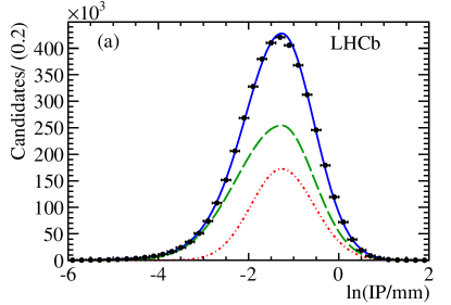
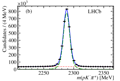
Figure 1: (a) The ln(IP/mm) distribution and (b) $p{{K}^{-}}{{\pi}^{+}}$ invariant mass for ${{\mathchar 28931\relax}^{+}_{c}}$ candidate combinations with a muon. The red (dashed-dotted) curves show the combinatorial ${{\mathchar 28931\relax}^{+}_{c}}$ background, the green (dashed) curves the ${{\mathchar 28931\relax}^{+}_{c}}$ from ${{\mathchar 28931\relax}^{0}_{b}}$ and the blue-solid curves the total yields.

Our goal is the study of the ground-state semileptonic decay ${{\mathchar 28931\relax}^{0}_{b}}\rightarrow{{\mathchar 28931\relax}^{+}_{c}}{\mu^{-}}{{\overline{\nu}}_{\mu}}$, thus we need to estimate the contributions from $\mathchar 28931\relax_{c}^{\ast+}$ decaying into ${{\mathchar 28931\relax}^{+}_{c}}\pi\pi$ states. Theoretical predictions suggest that the inclusive rate ${{\mathchar 28931\relax}^{0}_{b}}\rightarrow{{\mathchar 28931\relax}^{+}_{c}}{\mu^{-}}{{\overline{\nu}}_{\mu}}X$ is dominated by the exclusive channel ${{\mathchar 28931\relax}^{0}_{b}}\rightarrow{{\mathchar 28931\relax}^{+}_{c}}{\mu^{-}}{{\overline{\nu}}_{\mu}}$ [40, 41]. The residual contribution is expected to be accounted for by the ${{\mathchar 28931\relax}^{0}_{b}}\rightarrow\mathchar 28931\relax_{c}(2595)^{+}{\mu^{-}}{{\overline{\nu}}_{\mu}}$ and ${{\mathchar 28931\relax}^{0}_{b}}\rightarrow\mathchar 28931\relax_{c}(2625)^{+}{\mu^{-}}{{\overline{\nu}}_{\mu}}$ channels. Other modes, such as ${{\mathchar 28931\relax}^{0}_{b}}\rightarrow{{\mathchar 28934\relax}^{+}_{c}}{\mu^{-}}{{\overline{\nu}}_{\mu}}$, are suppressed in the static limit and to order $1/m_{Q}$, where $m_{Q}$ represents the heavy quark mass ($m_{c}$ or $m_{b}$) [42], with an additional stronger suppression factor of the order $(m_{d}-m_{u})/m_{c}$ rather than $(m_{d}-m_{u})/m_{\Lambda_{\rm QCD}}$ [9].

We use ${{\mathchar 28931\relax}^{0}_{b}}\rightarrow{{\mathchar 28931\relax}^{+}_{c}}{{\pi}^{+}}{{\pi}^{-}}{\mu^{-}}{{\overline{\nu}}_{\mu}}$ decays to infer contributions from the excited ${{\mathchar 28931\relax}^{+}_{c}}$ modes, where the ${{\mathchar 28931\relax}^{+}_{c}}$ candidates are selected as $p{{K}^{-}}{{\pi}^{+}}$ combinations whose invariant mass is within $\pm 20\mathrm{\,Me\kern-1.00006ptV}$ of the nominal ${{\mathchar 28931\relax}^{+}_{c}}$ mass. The ${{\mathchar 28931\relax}^{+}_{c}}{\mu^{-}}{{\overline{\nu}}_{\mu}}$ candidates are combined with pairs of opposite-charge pions that satisfy criteria similar to those used to select the pions from the ${{\mathchar 28931\relax}^{+}_{c}}$ decay. The minimum transverse momentum of these pions is required to be $0.2\mathrm{\,Ge\kern-1.00006ptV}$ and the transverse momentum of the ${{\mathchar 28931\relax}^{+}_{c}}{{\pi}^{+}}{{\pi}^{-}}$ system is required to be greater than $1.5\mathrm{\,Ge\kern-1.00006ptV}$. Lastly, the $\chi^{2}$ per degree of freedom of the vertex fit for the ${{\mathchar 28931\relax}^{+}_{c}}{{\pi}^{+}}{{\pi}^{-}}$ system must be smaller than 6.

The resulting spectrum, measured as the mass difference $m(p{{K}^{-}}{{\pi}^{+}}{{\pi}^{-}}{{\pi}^{+}})-m(p{{K}^{-}}{{\pi}^{+}})$ added to the known ${{\mathchar 28931\relax}^{+}_{c}}$ mass[14], is shown in Fig. 2. We see peaks corresponding to the $\mathchar 28931\relax_{c}(2595)^{+}$, $\mathchar 28931\relax_{c}(2625)^{+}$, $\mathchar 28931\relax_{c}(2765)^{+}$, and $\mathchar 28931\relax_{c}(2880)^{+}$ resonances. The $\mathchar 28931\relax_{c}(2595)^{+}$ is only a few MeV above the kinematic threshold and thus it is not well described by a Breit-Wigner function. The baseline fit for this resonance uses a PDF consisting of the sum of two bifurcated Gaussian functions. As a check, we use an S-wave relativistic Breit-Wigner convolved with a Gaussian function with standard deviation $\sigma=2$ MeV that accounts for the detector resolution. While the second parameterization is more accurate, the fits to the invariant mass spectra in different kinematic bins are more stable with the baseline parameterization. We fit the $\mathchar 28931\relax_{c}(2625)^{+}$ signal with a double Gaussian PDF with shared mean, as the natural width is expected to be well below the measured detector resolution. The shape of the combinatoric background PDF is inferred from wrong-sign (WS) candidates, where a ${{\pi}^{+}}{{\pi}^{+}}$ or ${{\pi}^{-}}{{\pi}^{-}}$ pair is combined with $\mathchar 28931\relax_{c}^{+}$ instead of ${{\pi}^{+}}{{\pi}^{-}}$. In addition, we observe peaks corresponding to two higher mass resonances, with masses and widths consistent with the $\mathchar 28931\relax_{c}(2765)^{+}$ and $\mathchar 28931\relax_{c}(2880)^{+}$ baryons[14]. In order to determine their yields, we fit the two signal peaks with single Gaussian PDFs with unconstrained masses and widths. The measured yields for the four ${{\mathchar 28931\relax}^{+}_{c}}$ final states, as well as the ${{\mathchar 28931\relax}^{+}_{c}}{\mu^{-}}{{\overline{\nu}}_{\mu}}X$ final state, are presented in Table 2.

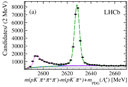
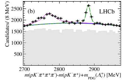
Figure 2: The mass difference $m(p{{K}^{-}}{{\pi}^{+}}{{\pi}^{+}}{{\pi}^{-}})-m(p{{K}^{-}}{{\pi}^{+}})$ added to the known ${{\mathchar 28931\relax}^{+}_{c}}$ mass, $m_{\rm PDG}({{\mathchar 28931\relax}^{+}_{c}})$  [14], for candidates with $p{{K}^{-}}{{\pi}^{+}}$ invariant mass within $\pm$20 MeV of the known ${{\mathchar 28931\relax}^{+}_{c}}$ mass in candidate semileptonic decays for the entire $w$ range: data are shown as black dots, the combinatoric background is shown as a blue solid line, and the gray histogram shows the WS spectrum, obtained by combining a ${{\pi}^{+}}{{\pi}^{+}}$ or ${{\pi}^{-}}{{\pi}^{-}}$ pair with ${{\mathchar 28931\relax}^{+}_{c}}$ instead of ${{\pi}^{+}}{{\pi}^{-}}$. The signal fits are identified as follows: (a) for $m<2700$ MeV, the $\mathchar 28931\relax_{c}(2595)^{+}$ as magenta dashed line, and the $\mathchar 28931\relax_{c}(2625)^{+}$ as green long-dashed line, (b) for $m>2700$ MeV, the $\mathchar 28931\relax_{c}(2765)^{+}$ as magenta dashed line, and the $\mathchar 28931\relax_{c}(2880)^{+}$ as green long-dashed line.

Table 2: Measured raw yields for the four $\mathchar 28931\relax_{c}^{\ast+}{\mu^{-}}{{\overline{\nu}}_{\mu}}$ final states and the inclusive ${{\mathchar 28931\relax}^{+}_{c}}{\mu^{-}}{{\overline{\nu}}_{\mu}}X$.

Final state	Yield
$\mathchar 28931\relax_{c}(2595)^{+}{\mu^{-}}{{\overline{\nu}}_{\mu}}$	08569 $\pm$ 144
$\mathchar 28931\relax_{c}(2625)^{+}{\mu^{-}}{{\overline{\nu}}_{\mu}}$	22965 $\pm$ 266
$\mathchar 28931\relax_{c}(2765)^{+}{\mu^{-}}{{\overline{\nu}}_{\mu}}$	02975 $\pm$ 225
$\mathchar 28931\relax_{c}(2880)^{+}{\mu^{-}}{{\overline{\nu}}_{\mu}}$	1602 $\pm$ 95
${{\mathchar 28931\relax}^{+}_{c}}{\mu^{-}}{{\overline{\nu}}_{\mu}}X$	0(2.74$\pm$0.02)$\times 10^{6}$

The measured contributions from the two heavier $\mathchar 28931\relax_{c}^{\ast+}$ final states, shown in Table 2, are smaller than those from ${{\mathchar 28931\relax}^{0}_{b}}\rightarrow\mathchar 28931\relax_{c}(2595)^{+}{\mu^{-}}{{\overline{\nu}}_{\mu}}$ and ${{\mathchar 28931\relax}^{0}_{b}}\rightarrow\mathchar 28931\relax_{c}(2625)^{+}{\mu^{-}}{{\overline{\nu}}_{\mu}}$ decays. No theoretical prediction for nonresonant ${{\mathchar 28931\relax}^{0}_{b}}\rightarrow{{\mathchar 28931\relax}^{+}_{c}}{{\pi}^{+}}{{\pi}^{-}}{\mu^{-}}{{\overline{\nu}}_{\mu}}X$ exists, but we estimate systematic uncertainties due to the subtraction of this component with an alternative fit of the ${{\mathchar 28931\relax}^{0}_{b}}\rightarrow{{\mathchar 28931\relax}^{+}_{c}}{{\pi}^{+}}{{\pi}^{-}}{\mu^{-}}{{\overline{\nu}}_{\mu}}X$ spectrum from candidate ${{\mathchar 28931\relax}^{0}_{b}}$ semileptonic decays, where we derive both the yield and shape of the combinatoric background from the WS sample.

The kinematical quantities ${q^{2}}$ and $w$ in the decay ${{\mathchar 28931\relax}^{0}_{b}}\rightarrow{{\mathchar 28931\relax}^{+}_{c}}{\mu^{-}}{{\overline{\nu}}_{\mu}}$ can be calculated if the magnitude of the ${{\mathchar 28931\relax}^{0}_{b}}$ momentum is known. The ${{\mathchar 28931\relax}^{0}_{b}}$ flight direction can be inferred from the primary and secondary vertex locations, and this input, combined with the constraints from energy and momentum conservation, implies the following relationship for $p_{{{\mathchar 28931\relax}^{0}_{b}}}$

$$\left[\left(\frac{\hat{p}_{{{\mathchar 28931\relax}^{0}_{b}}}\cdot\vec{p}_{{{\mathchar 28931\relax}^{+}_{c}}{\mu^{-}}}}{E_{{{\mathchar 28931\relax}^{+}_{c}}{\mu^{-}}}}\right)^{2}-1\right]p_{{{\mathchar 28931\relax}^{0}_{b}}}^{2}+\left[(m_{{{\mathchar 28931\relax}^{0}_{b}}}^{2}+m_{{{\mathchar 28931\relax}^{+}_{c}}{\mu^{-}}}^{2})\frac{\hat{p}_{{{\mathchar 28931\relax}^{0}_{b}}}\cdot\vec{p}_{{{\mathchar 28931\relax}^{+}_{c}}{\mu^{-}}}}{E^{2}_{{{\mathchar 28931\relax}^{+}_{c}}{\mu^{-}}}}\right]p_{{{\mathchar 28931\relax}^{0}_{b}}}$$ (6)

$$+\left[\left(\frac{(m_{{{\mathchar 28931\relax}^{0}_{b}}}^{2}+m_{{{\mathchar 28931\relax}^{+}_{c}}{\mu^{-}}}^{2})}{2E_{{{\mathchar 28931\relax}^{+}_{c}}{\mu^{-}}}}\right)^{2}-m_{{{\mathchar 28931\relax}^{0}_{b}}}^{2}\right]=0,$$

where the unit vector $\hat{p}_{{{\mathchar 28931\relax}^{0}_{b}}}$ is the direction of the ${{\mathchar 28931\relax}^{0}_{b}}$ baryon, $\vec{p}_{{{\mathchar 28931\relax}^{+}_{c}}{\mu^{-}}}$ is the momentum of the ${{\mathchar 28931\relax}^{+}_{c}}{\mu^{-}}$ pair, $E_{{{\mathchar 28931\relax}^{+}_{c}}{\mu^{-}}}$ is the energy of the ${{\mathchar 28931\relax}^{+}_{c}}{\mu^{-}}$ pair, $m_{{{\mathchar 28931\relax}^{+}_{c}}{\mu^{-}}}$ is the invariant mass of the ${{\mathchar 28931\relax}^{+}_{c}}{\mu^{-}}$ pair, $m_{{{\mathchar 28931\relax}^{0}_{b}}}$ is the nominal mass of the ${{\mathchar 28931\relax}^{0}_{b}}$ baryon, and ${{\mathchar 28931\relax}^{+}_{c}}$ identifies the $p{{K}^{-}}{{\pi}^{+}}$ combination. This is a quadratic equation, reflecting the lack of knowledge of the neutrino orientation in the ${{\mathchar 28931\relax}^{0}_{b}}$ rest frame with respect to the ${{\mathchar 28931\relax}^{0}_{b}}$ direction in the laboratory. The solution corresponding to the lower value of $p_{{{\mathchar 28931\relax}^{0}_{b}}}$, which is correct between 50% and 60% of the time depending upon the kinematics of the final state, is chosen in the ${q^{2}}$ and $w$ determination as simulation studies have shown that this choice introduces the smallest bias. The $w$ resolution is estimated from simulated data in different $w$ intervals. The distributions of differences between reconstructed and generated $w$ are fitted with double-Gaussian functions and the effective standard deviations are found to be between 0.01 and 0.05. The overall $w$ resolution is estimated with a fit with a triple-Gaussian function, and has an effective standard deviation $\sigma$ equal to $0.028$.

4 The spectral distribution ${dN_{\rm corr}/dw({{\mathchar 28931\relax}^{0}_{b}}\rightarrow{{\mathchar 28931\relax}^{+}_{c}}{\mu^{-}}{{\overline{\nu}}_{\mu}})}$

The ${{\mathchar 28931\relax}^{0}_{b}}\rightarrow{{\mathchar 28931\relax}^{+}_{c}}{\mu^{-}}{{\overline{\nu}}_{\mu}}X$ candidates are separated into 14 equal-size bins of reconstructed $w$ in the full kinematic range $1\leq w\leq 1.43$. The parameters of the PDFs describing the signal and background components are determined from the fit to the overall $pK^{-}{{\pi}^{+}}$ mass spectrum. The contributions from semileptonic decays including higher-mass baryons in the final state is evaluated by fitting the ${{\mathchar 28931\relax}^{+}_{c}}{{\pi}^{+}}{{\pi}^{-}}$ mass spectra with two different methods. In the first, we fit for the four resonances shown in Fig. 2 using a PDF derived from the WS sample to model the background, and then use the simulation to correct for efficiency. In the second, we determine the signal yields of the $\mathchar 28931\relax_{c}^{\ast+}$ states by subtracting the WS background and treating the residual smooth component of the spectrum as originating from a semileptonic decay ${{\mathchar 28931\relax}^{0}_{b}}\rightarrow{{\mathchar 28931\relax}^{+}_{c}}{\mu^{-}}{{\overline{\nu}}_{\mu}}X$. The second method provides an estimate of the systematic uncertainty introduced by the contribution from nonresonant ${{\mathchar 28931\relax}^{+}_{c}}{{\pi}^{+}}{{\pi}^{-}}$ components of the hadron spectrum, as the smooth component of this spectrum is likely to comprise also combinatoric background.

Next, we correct the raw ${{\mathchar 28931\relax}^{+}_{c}}{\mu^{-}}{{\overline{\nu}}_{\mu}}X$ and ${{\mathchar 28931\relax}^{+}_{c}}{{\pi}^{+}}{{\pi}^{-}}{\mu^{-}}{{\overline{\nu}}_{\mu}}X$ signal yields for the corresponding software trigger efficiencies, which are derived with a data-driven method [30], based on the determination of ${{\mathchar 28931\relax}^{+}_{c}}{\mu^{-}}{{\overline{\nu}}_{\mu}}X$ events where a positive trigger decision is provided by the signal candidates, and events where the trigger decision is independent of the signal. Then we subtract the raw yields reported in Table 2, scaled by the corresponding efficiency ratios $\varepsilon({{\mathchar 28931\relax}^{0}_{b}}\rightarrow{{\mathchar 28931\relax}^{+}_{c}}{\mu^{-}}{{\overline{\nu}}_{\mu}}X)\over\varepsilon({{\mathchar 28931\relax}^{0}_{b}}\rightarrow{{\mathchar 28931\relax}^{+}_{c}}{{\pi}^{+}}{{\pi}^{-}}{\mu^{-}}{{\overline{\nu}}_{\mu}}X)$, from the corrected ${{\mathchar 28931\relax}^{+}_{c}}{\mu^{-}}{{\overline{\nu}}_{\mu}}X$ yields. These ratios are derived from ${{\mathchar 28931\relax}^{0}_{b}}\rightarrow\mathchar 28931\relax_{c}(2595)^{+}{\mu^{-}}{{\overline{\nu}}_{\mu}}$ and ${{\mathchar 28931\relax}^{0}_{b}}\rightarrow\mathchar 28931\relax_{c}(2625)^{+}{\mu^{-}}{{\overline{\nu}}_{\mu}}$ simulations. The higher mass yields are scaled by an average of these two corrections, as no model for these semileptonic decays is available. These corrections account for the efficiency loss due to the reconstruction of the additional pion pairs, as well as for the unseen ${{\mathchar 28931\relax}^{0}_{b}}\rightarrow{{\mathchar 28931\relax}^{+}_{c}}{{\pi}^{0}}{{\pi}^{0}}{\mu^{-}}{{\overline{\nu}}_{\mu}}X$ decay and are only mildly dependent upon the invariant mass of the final state. The expectation is that ${{\mathchar 28931\relax}^{0}_{b}}\rightarrow{{\mathchar 28931\relax}^{+}_{c}}{{\pi}^{+}}{{\pi}^{-}}{\mu^{-}}{{\overline{\nu}}_{\mu}}$ accounts for two-thirds of the inclusive dipion final state. We have checked this prediction by studying the inclusive final states ${{\mathchar 28934\relax}^{++}_{c}}{\mu^{-}}{{\overline{\nu}}_{\mu}}X$, ${{\mathchar 28934\relax}^{+}_{c}}{\mu^{-}}{{\overline{\nu}}_{\mu}}X$, and ${{\mathchar 28934\relax}^{0}_{c}}{\mu^{-}}{{\overline{\nu}}_{\mu}}X$. Taking into account the difference in the $\mathchar 28931\relax_{c}^{+}{{\pi}^{+}}{{\pi}^{-}}{\mu^{-}}{{\overline{\nu}}_{\mu}}X$ and $\mathchar 28931\relax_{c}^{+}{{\pi}^{0}}{\mu^{-}}{{\overline{\nu}}_{\mu}}X$ detection efficiencies, estimated with simulations, we measure the ratio $R=N(\mathchar 28931\relax_{c}^{+}{{\pi}^{+}}{{\pi}^{-}})/N(\mathchar 28931\relax_{c}^{+}{{\pi}^{+}}{{\pi}^{-}}+\mathchar 28931\relax_{c}^{+}{{\pi}^{0}}{{\pi}^{0}})$ with

$$R=\frac{N({{\mathchar 28934\relax}^{++}_{c}})+N({{\mathchar 28934\relax}^{0}_{c}})}{N({{\mathchar 28934\relax}^{++}_{c}})+N({{\mathchar 28934\relax}^{0}_{c}})+N({{\mathchar 28934\relax}^{+}_{c}})\cdot[\varepsilon(\mathchar 28931\relax_{c}^{+}{{\pi}^{+}}{{\pi}^{-}}\mu)/\varepsilon(\mathchar 28931\relax_{c}^{+}{{\pi}^{0}}\mu)]},$$ (7)

where $N({{\mathchar 28934\relax}^{++}_{c}})$ and $N({{\mathchar 28934\relax}^{0}_{c}})$ are the detected yields for the final states ${{\mathchar 28934\relax}^{++}_{c}}{{\pi}^{-}}\mu\nu$ and ${{\mathchar 28934\relax}^{0}_{c}}{{\pi}^{+}}\mu\nu$, $N({{\mathchar 28934\relax}^{+}_{c}})$ is the detected yield for the final state ${{\mathchar 28934\relax}^{+}_{c}}\mu\nu X$ and $\varepsilon(\mathchar 28931\relax_{c}^{+}{{\pi}^{+}}{{\pi}^{-}}\mu)/\varepsilon(\mathchar 28931\relax_{c}^{+}{{\pi}^{0}}\mu)$ is the ratio between the reconstruction efficiencies of these final states calculated with simulation. A simulation study gives $\varepsilon(\mathchar 28931\relax_{c}^{+}{{\pi}^{+}}{{\pi}^{-}}\mu)/\varepsilon(\mathchar 28931\relax_{c}^{+}{{\pi}^{0}}\mu)=25.9\pm 2.7$, where the uncertainty reflects the limited sample size of the simulation. We obtain $R=0.63\pm 0.14$, where the statistical uncertainty is due to limited ${{\pi}^{0}}$ reconstruction efficiency, consistent with the expectation $R=2/3$, and a negligible ${{\mathchar 28934\relax}^{+}_{c}}{\mu^{-}}{{\overline{\nu}}_{\mu}}$ component in the denominator of Eq. 7.

The ${{\mathchar 28931\relax}^{0}_{b}}\rightarrow{{\mathchar 28931\relax}^{+}_{c}}{\mu^{-}}{{\overline{\nu}}_{\mu}}$ spectrum $dN_{\rm meas}/dw$ is then unfolded to account for the detector resolution and other $w$ smearing effects such as the possible choice of the wrong solution of Eq. 6. The procedure adopted is based on the single value decomposition (SVD) method [43] using the RooUnfold package[44]. We choose to divide the unfolded spectrum $dN_{\rm u}/dw$ into seven $w$ bins, to be consistent with the recommendation of Ref. [45] to divide the measured spectrum into a number of bins at least twice as many as the ones in the corrected spectrum. The SVD method includes a regularization procedure that depends upon a parameter $k$[43], ranging between unity and the number of degrees of freedom, in our case 14. Simulation studies demonstrate that $k=4$ is optimal in our case. Variations associated with different choices of $k$ have been studied and are included in the systematic uncertainties. We have performed closure tests with different simulation models of the ${{\mathchar 28931\relax}^{0}_{b}}\rightarrow{{\mathchar 28931\relax}^{+}_{c}}{\mu^{-}}{{\overline{\nu}}_{\mu}}$ dynamics, and verified that this unfolding procedure does not bias the reconstructed distribution. The spectra before and after unfolding are shown in Fig. 3. Finally, using simulated samples of signal events, we correct the unfolded spectrum for $w$-dependent acceptance and selection efficiency to obtain the distribution $dN_{\rm corr}/dw$. Various kinematic distributions have been studied in simulation and data and we find that they are all in good agreement.

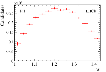
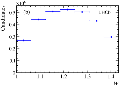
Figure 3: The spectra (a) $dN_{\rm meas}/dw$ before unfolding and (b) $dN_{\rm u}/dw$ after unfolding, for the decay ${{\mathchar 28931\relax}^{0}_{b}}\rightarrow{{\mathchar 28931\relax}^{+}_{c}}{\mu^{-}}{{\overline{\nu}}_{\mu}}$. The latter spectrum is then corrected for acceptance and reconstruction efficiency and fitted to the IW function $\xi_{B}(w)$ with the procedure discussed in the text.

5 The shape of $\xi_{B}(w)$ for ${{\mathchar 28931\relax}^{0}_{b}}\rightarrow{{\mathchar 28931\relax}^{+}_{c}}{\mu^{-}}{{\overline{\nu}}_{\mu}}$ decays

In order to determine the shape of the Isgur-Wise function $\xi_{B}(w)$, we use the square root of $dN_{\rm corr}/dw$ divided by the kinematic factor $K$($\langle w\rangle$), defined in Eq. 4, evaluated at the midpoint in the seven unfolded $w$ bins. We derive the IW shape with a $\chi^{2}$ fit, where the $\chi^{2}$ is formed using the full covariance matrix of $dN_{\rm corr}/dw$.

We use various functional forms to extract the slope, $\rho^{2}$, and curvature, $\sigma^{2}$, of $\xi_{B}(w)$. The first functional form is motivated by the 1/$N_{c}$ expansion [46], where $N_{c}$ represents the number of colors, and has an exponential shape parameterized as

$$\xi_{B}(w)=\exp[-\rho^{2}(w-1)].$$ (8)

The second functional form, the so called “dipole” IW function, which is more consistent with sum-rule bounds [17], is given by

$$\xi_{B}(w)=\left(\frac{2}{w+1}\right)^{2\rho^{2}}.$$ (9)

Finally, we can use a simple Taylor series expansion of the Isgur-Wise function and fit for the slope and curvature parameters using the Taylor series expansion introduced in Eq. 5. Figure 4 shows the measured $\xi_{B}(w)$ and the fit results with this parameterization. Table 3 summarizes the slope and curvature at zero recoil obtained with the three fit models. Note that the curvature is an independent parameter only in the last fit, while in the first two models it is related to the second derivative of the IW function.

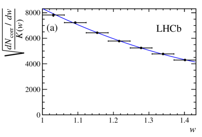
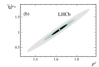
Figure 4: (a) The Isgur-Wise function fit for the decay ${{\mathchar 28931\relax}^{0}_{b}}\rightarrow{{\mathchar 28931\relax}^{+}_{c}}{\mu^{-}}\nu$ with a Taylor series expansion in $(w-1)$ up to second order. The black dots show the data and the solid (blue) line shows the fitted function with the second-order Taylor series expansion model. The vertical scale is in arbitrary units. (b) The correlation between slope $\rho^{2}$ and curvature $\sigma^{2}/2$: the three ellipses correspond to the 1$\sigma$, 2$\sigma$, and 4$\sigma$ contours.

Table 3: Summary of the values for the slope and curvature of the Isgur-Wise function with different parameterizations. The quoted uncertainties are statistical only. The models marked with “*” have only the slope at zero recoil as a free parameter, thus the curvature is derived from the fitted $\rho^{2}$.

Shape	$\rho^{2}$	$\sigma^{2}$	correlation coefficient	$\chi^{2}$/ DOF
Exponential*	1.65 $\pm$ 0.03	2.72 $\pm$ 0.10	100%	5.3/5
Dipole*	1.82 $\pm$ 0.03	4.22 $\pm$ 0.12	100%	5.3/5
Taylor series	1.63 $\pm$ 0.07	2.16 $\pm$ 0.34	97%	4.5/4

As the slope of the IW function is the most relevant quantity to determine $|{V_{{c}{b}}}|$ in the framework of HQET [13], we focus our studies on the systematic uncertainties on this parameter. We consider several sources of systematic uncertainties, which are listed in Table 4. The first two are determined by changing the fit models for ${{\mathchar 28931\relax}^{+}_{c}}$ and $\mathchar 28931\relax_{c}(2595)^{+}$ and $\mathchar 28931\relax_{c}(2625)^{+}$ signal shapes in the corresponding candidate mass spectra. The software trigger efficiency uncertainty is estimated by using an alternative procedure to evaluate this efficiency using the trigger emulation in the LHCb simulation. In order to assess systematics associated with the bin size, we perform the analysis with different binning choices. The sensitivity to the ${{\mathchar 28931\relax}^{0}_{b}}\rightarrow{{\mathchar 28931\relax}^{+}_{c}}{\mu^{-}}{{\overline{\nu}}_{\mu}}$ form factor modeling is assessed by reweighting the simulated $w$ spectra to correspond to different $\xi_{B}$ functions with slopes ranging from 1.5 to 1.7. The “phase space averaging” sensitivity is estimated by comparing the fit to the expression for $dN_{\rm corr}/dw$ with the fit to $1/K(\langle w\rangle)\sqrt{dN_{\rm corr}/dw}$. The uncertainty associated with the ${{\mathchar 28931\relax}^{0}_{b}}\rightarrow\mathchar 28931\relax_{c}^{\ast+}{\mu^{-}}{{\overline{\nu}}_{\mu}}$ modeling is evaluated by changing the relative fraction of ${{\mathchar 28931\relax}^{+}_{c}}{{\pi}^{+}}{{\pi}^{-}}$ versus ${{\mathchar 28931\relax}^{+}_{c}}{{\pi}^{0}}{{\pi}^{0}}$ of the $\mathchar 28931\relax_{c}^{\ast+}$ spectrum by $\pm$ 20%. Finally, we use the alternative evaluation of the fraction of ${{\mathchar 28931\relax}^{0}_{b}}\rightarrow{{\mathchar 28931\relax}^{+}_{c}}{{\pi}^{+}}{{\pi}^{-}}{\mu^{-}}{{\overline{\nu}}_{\mu}}$ which includes the maximum possible nonresonant component to assess the sensitivity to residual $\mathchar 28931\relax_{c}^{\ast+}$ components in the subtracted spectrum. The total systematic uncertainty in $\rho^{2}$ is 0.08.

The value of $\rho^{2}$ obtained from the Taylor series expansion is

$$\rho^{2}=1.63\pm 0.07\pm 0.08,$$

which is consistent with Lattice calculations [23], QCD sum rules [22], and relativistic quark model [21] expectations. The measured slope is compatible with theoretical predictions and with the bound $\rho^{2}\geq$ 3/4[16]. The measured curvature $\sigma^{2}$ is compatible within uncertainties with the lower bound $\sigma^{2}\geq 3/5[\rho^{2}+(\rho^{2})^{2}]$ [18].

Table 4: Summary of the systematic uncertainties on the slope parameter $\rho^{2}$. The total uncertainty is obtained by adding the individual components in quadrature.

Source	$\sigma(\rho^{2})$
Signal fit for ${{\mathchar 28931\relax}^{+}_{c}}$	$0.02$
Signal PDF for $\mathchar 28931\relax_{c}^{\ast+}$	$0.02$
Software trigger efficiency	$0.02$
$w$ binning	$0.03$
SVD unfolding regularization	$0.03$
Phase space averaging	0.03
${{\mathchar 28931\relax}^{0}_{b}}\rightarrow{{\mathchar 28931\relax}^{+}_{c}}{\mu^{-}}{{\overline{\nu}}_{\mu}}$ modeling	$0.03$
${{\mathchar 28931\relax}^{0}_{b}}\rightarrow\mathchar 28931\relax_{c}^{\ast+}{\mu^{-}}{{\overline{\nu}}_{\mu}}$ modeling	$0.03$
Additional components of the semileptonic spectrum	$0.02$
${{\mathchar 28931\relax}^{0}_{b}}$ kinematic dependencies	0.02
Total	$0.08$

6 Comparison with unquenched lattice predictions

The lattice QCD calculation in Ref. [19] uses a helicity-based description of the six form factors governing ${{\mathchar 28931\relax}^{0}_{b}}\rightarrow{\mathchar 28931\relax}$ transitions introduced in Ref. [47]. The calculation uses state-of-the-art techniques encompassing the entire ${q^{2}}$ region. The stated uncertainties on the predicted width are therefore larger than what is expected in a high-${q^{2}}$ region, but remain rather small, namely 6.3%. This corresponds to a 3.2% theoretical uncertainty on $|{V_{{c}{b}}}|$, thus raising the prospect of an additional precise independent determination of $|{V_{{c}{b}}}|$.

The simplest check on this theoretical prediction consists of a comparison of the predicted shape of $d\Gamma/d{q^{2}}$ and the measured data. Thus we measure the distribution $dN_{\rm corr}/d{q^{2}}$ with the same procedure adopted to derive $dN_{\rm corr}/dw$, including efficiency corrections and the unfolding procedure, with the same number of bins used to determine the raw and unfolded yields. We produce seven corrected yields and their associated covariance matrix, where the nondiagonal terms are related to the unfolding procedure. We then perform a $\chi^{2}$ fit to the seven experimental $dN_{\rm corr}/d{q^{2}}$ data points using the theoretical functional shape given in Eq. 85 of Ref. [19], which also provides the nominal values of the form factor parameters, and thus we leave only the relative normalization floating. This fit uses a covariance matrix that combines experimental and theoretical uncertainties, which yields a $\chi^{2}$ equal to 1.32 for 6 degrees of freedom, and a corresponding p-value of 97%. This shows that the predicted shape is in good agreement with our measurement.

The form factor decomposition in Ref. [19] does not allow a straightforward extrapolation to the HQET limit of infinite heavy-quark masses. However, we know that in the static limit all the form factors are proportional to a single universal function. In order to assess how well our data are consistent with the static limit, we perform a second $\chi^{2}$ fit assuming that all the form factors are proportional to a single $z$-expansion function [48]. Fits with different pole masses used in the six form factors determined in Ref. [19] are performed. The overall shape does not change appreciably; the pole mass of $6.768\mathrm{\,Ge\kern-1.00006ptV}$ is preferred. The two fit parameters are the coefficients $a_{0}$ and $a_{1}$, giving the strength of the first two terms in the $z$-expansion. The resulting fitted shape is shown in Fig. 5. This fit has a $\chi^{2}$ equal to 1.85 for 5 degrees of freedom, with a corresponding p-value of 87%. Note that the shape obtained with a single form-factor is very similar to the one predicted in Ref. [19]. This is consistent with the HQET prediction [15] that the shape of the differential distribution is well described by the static approximation, modulo a scale correction of the order of 10%, reflecting higher-order contributions. Further details of this fit and the fit using the Lattice QCD calculation can be found in the Appendix.

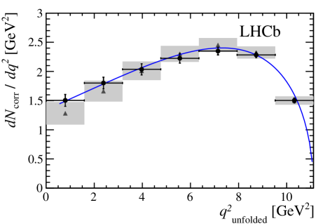
Figure 5: Comparison between the fit to the seven experimental data points using either the Lattice QCD calculation of Ref. [19], shown as grey points with a shaded area corresponding to the binned 1$\sigma$ theory uncertainty, or a single form factor fit in the $z$-expansion, shown as the solid blue curve. The data points, modulo a scale factor, are shown as black points with error bars.

7 Conclusions

A precise measurement of the shape of the Isgur-Wise function describing the semileptonic decay ${{\mathchar 28931\relax}^{0}_{b}}\!\rightarrow{{\mathchar 28931\relax}^{+}_{c}}{\mu^{-}}{{\overline{\nu}}_{\mu}}$ has been performed. The measured slope is consistent with theoretical models and the bound $\rho^{2}\geq 3/4$ [16]. The measured curvature $\sigma^{2}$ is consistent with the lower-bound constraint $\sigma^{2}\geq 3/5[\rho^{2}+(\rho^{2})^{2}]$ [18]. The shape of $d\Gamma/d{q^{2}}$ is studied and found to be well described by the unquenched lattice QCD prediction of Ref. [19], as well as by a single form-factor parameterization. Further studies with a suitable normalization channel will lead to a precise independent determination of the CKM parameter $|{V_{{c}{b}}}|$.

Appendix I: Analytical expression for $d\Gamma/d{q^{2}}$

This Appendix describes the formalism used in the $d\Gamma/d{q^{2}}$ fits. In particular, we give the expression of $d\Gamma/d{q^{2}}$ in terms of the form factor basis chosen in Ref. [19], the so-called “helicity form factors”. In addition, we show the corresponding expression used to model the static limit.

Table 5: Masses of the relevant form factor poles in the physical limit (in GeV).

$f$		$J^{P}$		$m_{\rm pole}^{f}({{\mathchar 28931\relax}^{0}_{b}}\rightarrow\Lambda_{c})~{}[\mathrm{\,Ge\kern-1.00006ptV}]$
$f_{+}$, $f_{\perp}$		$1^{-}$		6.332
$f_{0}$		$0^{+}$		6.725
$g_{+}$, $g_{\perp}$		$1^{+}$		6.768
$g_{0}$		$0^{-}$		6.276

The Lattice QCD calculations reported in Ref. [19] predict the differential decay width $d\Gamma({{\mathchar 28931\relax}^{0}_{b}}\rightarrow{{\mathchar 28931\relax}^{+}_{c}}{\mu^{-}}{{\overline{\nu}}_{\mu}})/d{q^{2}}$ as follows

$$\frac{\mathrm{d}\Gamma}{\mathrm{d}q^{2}} = \frac{G_{F}^{2}|{V_{{c}{b}}}|^{2}\sqrt{s_{+}s_{-}}}{768\pi^{3}m_{{{\mathchar 28931\relax}^{0}_{b}}}^{3}}\left(1-\frac{m_{\ell}^{2}}{q^{2}}\right)^{2}$$ (10)

$$\times\Bigg{\{}4\left(m_{\ell}^{2}+2q^{2}\right)\left(s_{+}\left[g_{\perp}\right({q^{2}})]^{2}+s_{-}\left[f_{\perp}({q^{2}})\right]^{2}\right)$$

$$\hskip 8.61108pt+2\frac{m_{\ell}^{2}+2q^{2}}{q^{2}}\left(s_{+}\left[\left(m_{{{\mathchar 28931\relax}^{0}_{b}}}-m_{X}\right)g_{+}({q^{2}})\right]^{2}+s_{-}\left[\left(m_{{{\mathchar 28931\relax}^{0}_{b}}}+m_{X}\right)f_{+}({q^{2}})\right]^{2}\right)$$

$$\hskip 8.61108pt+\frac{6m_{\ell}^{2}}{q^{2}}\left(s_{+}\left[\left(m_{{{\mathchar 28931\relax}^{0}_{b}}}-m_{X}\right)f_{0}({q^{2}})\right]^{2}+s_{-}\left[\left(m_{{{\mathchar 28931\relax}^{0}_{b}}}+m_{X}\right)g_{0}({q^{2}})\right]^{2}\right)\Bigg{\}},$$

where $g_{\perp}$, $f_{\perp}$, $g_{+}$, $f_{+}$, $g_{0}$, and $f_{0}$ represent the six form factors necessary to describe this decay, $X\equiv\Lambda_{c}$ denotes the final-state baryon, $m_{\ell}$ represents the mass of the muon, ${q^{2}}$ is the squared four-momentum transfer between the heavy baryons, and

$$s_{\pm}=(m_{{{\mathchar 28931\relax}^{0}_{b}}}\pm m_{X})^{2}-q^{2}.$$ (11)

The six form factors are cast in terms of the $z$-expansion [48] up to first order, and have the functional form

$$f({q^{2}})=\frac{1}{1-{q^{2}}/(m^{f}_{\rm pole})^{2}}\times\left[a_{0}^{f}+a_{1}^{f}z^{f}({q^{2}})\right],$$ (12)

where $z^{f}({q^{2}})$ is given by

$$z^{f}(q^{2}) = \frac{\sqrt{t^{f}_{+}-q^{2}}-\sqrt{t_{+}^{f}-t_{0}}}{\sqrt{t_{+}^{f}-q^{2}}+\sqrt{t_{+}^{f}-t_{0}}},$$ (13)

$$t_{0} = (m_{{{\mathchar 28931\relax}^{0}_{b}}}-m_{X})^{2},$$ (14)

and $t_{+}^{f}$ is given by

$$t_{+}^{f}=(m^{f}_{\rm pole})^{2},$$ (15)

and the pole masses used in the calculations are shown in Table 5. The parameters $a_{0}^{f}$ and $a_{1}^{f}$ for the six form factors describing this decay are given in Table VIII of Ref. [19].

In the static limit all the helicity form factors are proportional to a single universal function. Thus, we use a common $z$-expansion parameterization

$$\frac{\mathrm{d}\Gamma}{\mathrm{d}q^{2}} = \frac{G_{F}^{2}|{V_{{c}{b}}}|^{2}\sqrt{s_{+}s_{-}}}{768\pi^{3}m_{{{\mathchar 28931\relax}^{0}_{b}}}^{3}}\left(1-\frac{m_{\ell}^{2}}{q^{2}}\right)^{2}g_{\perp}^{2}({q^{2}})$$ (16)

$$\times\Bigg{\{}4\left(m_{\ell}^{2}+2q^{2}\right)\left(s_{+}+s_{-}\right)$$

$$\hskip 8.61108pt+\frac{4}{q^{2}}\left[s_{+}\left(m_{{{\mathchar 28931\relax}^{0}_{b}}}-m_{X}\right)^{2}+s_{-}\left(m_{{{\mathchar 28931\relax}^{0}_{b}}}+m_{X}\right)^{2}\right]\left[2m_{\ell}^{2}+q^{2}\right]\Bigg{\}},$$

where the choice of $g_{\perp}$ reflects the choice of the pole mass used in the single $z$-expansion fit given in Sect. 6. We have performed the fits with various choices of pole masses and examined the effects on the shape $d\Gamma/d{q^{2}}$ and found the shape did not vary significantly, though it was found that the parameters defining $g_{\perp}$ yielded the optimal fit. In this case, the fit parameters are the coefficients $a_{0}$ and $a_{1}$ in the $z$-expansion parameterization of $g_{\perp}({q^{2}})$, which has the form shown in Eq. 12.

Appendix II: Measured normalized spectra $dN_{\rm corr}/d{q^{2}}$ and associated covariance matrix

In this appendix we report the seven measured data points $dN_{\rm corr}/d{q^{2}}$ and the corresponding covariance matrix, shown in Table 6 and Table 7 respectively.

Table 6: Measured normalized yields $dN_{\rm corr}({{\mathchar 28931\relax}^{0}_{b}}\rightarrow{{\mathchar 28931\relax}^{+}_{c}}{\mu^{-}}{{\overline{\nu}}_{\mu}})/d{q^{2}}$ .

${q^{2}}$ [GeV2]	$dN_{\rm corr}/d{q^{2}}$
0.80	1.50 $\pm$ 0.10
2.38	1.80 $\pm$ 0.10
3.97	2.04 $\pm$ 0.10
5.56	2.23 $\pm$ 0.08
7.14	2.35 $\pm$ 0.07
8.73	2.28 $\pm$ 0.05
10.32	1.50 $\pm$ 0.04

Table 7: Covariance matrix of the measured normalized yields ${\rm Cov}[dN_{\rm corr}({{\mathchar 28931\relax}^{0}_{b}}\rightarrow{{\mathchar 28931\relax}^{+}_{c}}{\mu^{-}}{{\overline{\nu}}_{\mu}})/d{q^{2}}$] .

${q^{2}}$ [GeV2]	$dN_{\rm corr}/d{q^{2}}$
0.80	0.0103	0.0052	-0.0032	-0.0033	-0.0009	0.0004	0.0005
2.38	0.0052	0.0100	0.0044	0.0011	-0.0002	-0.0006	0.0002
3.97	-0.0032	0.0044	0.0090	0.0048	0.0004	-0.0013	-0.0007
5.56	-0.0035	-0.0011	0.0048	0.0070	0.0031	-0.0006	-0.0013
7.14	-0.0009	-0.0019	-0.0004	0.0031	0.0044	0.0015	0.0006
8.73	0.0004	-0.0006	-0.0013	-0.0006	0.0015	0.0023	0.0013
10.32	0.0005	0.0002	-0.0007	-0.0013	-0.0006	0.0013	0.0018

LHCb collaboration: R. Aaij, B. Adeva, M. Adinolfi, Z. Ajaltouni, S. Akar, J. Albrecht, F. Alessio, M. Alexander, A. Alfonso Albero, S. Ali, G. Alkhazov, P. Alvarez Cartelle, A.A. Alves Jr, S. Amato, S. Amerio, Y. Amhis, L. An, L. Anderlini, G. Andreassi, M. Andreotti, J.E. Andrews, R.B. Appleby, F. Archilli, P. d’Argent, J. Arnau Romeu, A. Artamonov, M. Artuso, E. Aslanides, G. Auriemma, M. Baalouch, I. Babuschkin, S. Bachmann, J.J. Back, A. Badalov, C. Baesso, S. Baker, V. Balagura, W. Baldini, A. Baranov, R.J. Barlow, C. Barschel, S. Barsuk, W. Barter, F. Baryshnikov, V. Batozskaya, V. Battista, A. Bay, L. Beaucourt, J. Beddow, F. Bedeschi, I. Bediaga, A. Beiter, L.J. Bel, N. Beliy, V. Bellee, N. Belloli, K. Belous, I. Belyaev, E. Ben-Haim, G. Bencivenni, S. Benson, S. Beranek, A. Berezhnoy, R. Bernet, D. Berninghoff, E. Bertholet, A. Bertolin, C. Betancourt, F. Betti, M.-O. Bettler, M. van Beuzekom, Ia. Bezshyiko, S. Bifani, P. Billoir, A. Birnkraut, A. Bitadze, A. Bizzeti, M. Bjørn, T. Blake, F. Blanc, J. Blouw, S. Blusk, V. Bocci, T. Boettcher, A. Bondar, N. Bondar, W. Bonivento, I. Bordyuzhin, A. Borgheresi, S. Borghi, M. Borisyak, M. Borsato, F. Bossu, M. Boubdir, T.J.V. Bowcock, E. Bowen, C. Bozzi, S. Braun, T. Britton, J. Brodzicka, D. Brundu, E. Buchanan, C. Burr, A. Bursche, J. Buytaert, W. Byczynski, S. Cadeddu, H. Cai, R. Calabrese, R. Calladine, M. Calvi, M. Calvo Gomez, A. Camboni, P. Campana, D.H. Campora Perez, L. Capriotti, A. Carbone, G. Carboni, R. Cardinale, A. Cardini, P. Carniti, L. Carson, K. Carvalho Akiba, G. Casse, L. Cassina, L. Castillo Garcia, M. Cattaneo, G. Cavallero, R. Cenci, D. Chamont, M. Charles, Ph. Charpentier, G. Chatzikonstantinidis, M. Chefdeville, S. Chen, S.F. Cheung, S.-G. Chitic, V. Chobanova, M. Chrzaszcz, A. Chubykin, P. Ciambrone, X. Cid Vidal, G. Ciezarek, P.E.L. Clarke, M. Clemencic, H.V. Cliff, J. Closier, V. Coco, J. Cogan, E. Cogneras, V. Cogoni, L. Cojocariu, P. Collins, T. Colombo, A. Comerma-Montells, A. Contu, A. Cook, G. Coombs, S. Coquereau, G. Corti, M. Corvo, C.M. Costa Sobral, B. Couturier, G.A. Cowan, D.C. Craik, A. Crocombe, M. Cruz Torres, R. Currie, C. D’Ambrosio, F. Da Cunha Marinho, E. Dall’Occo, J. Dalseno, A. Davis, O. De Aguiar Francisco, K. De Bruyn, S. De Capua, M. De Cian, J.M. De Miranda, L. De Paula, M. De Serio, P. De Simone, C.T. Dean, D. Decamp, L. Del Buono, H.-P. Dembinski, M. Demmer, A. Dendek, D. Derkach, O. Deschamps, F. Dettori, B. Dey, A. Di Canto, P. Di Nezza, H. Dijkstra, F. Dordei, M. Dorigo, A. Dosil Suárez, L. Douglas, A. Dovbnya, K. Dreimanis, L. Dufour, G. Dujany, K. Dungs, P. Durante, R. Dzhelyadin, M. Dziewiecki, A. Dziurda, A. Dzyuba, N. Déléage, S. Easo, M. Ebert, U. Egede, V. Egorychev, S. Eidelman, S. Eisenhardt, U. Eitschberger, R. Ekelhof, L. Eklund, S. Ely, S. Esen, H.M. Evans, T. Evans, A. Falabella, N. Farley, S. Farry, R. Fay, D. Fazzini, L. Federici, D. Ferguson, G. Fernandez, P. Fernandez Declara, A. Fernandez Prieto, F. Ferrari, F. Ferreira Rodrigues, M. Ferro-Luzzi, S. Filippov, R.A. Fini, M. Fiore, M. Fiorini, M. Firlej, C. Fitzpatrick, T. Fiutowski, F. Fleuret, K. Fohl, M. Fontana, F. Fontanelli, D.C. Forshaw, R. Forty, V. Franco Lima, M. Frank, C. Frei, J. Fu, W. Funk, E. Furfaro, C. Färber, E. Gabriel, A. Gallas Torreira, D. Galli, S. Gallorini, S. Gambetta, M. Gandelman, P. Gandini, Y. Gao, L.M. Garcia Martin, J. García Pardiñas, J. Garra Tico, L. Garrido, P.J. Garsed, D. Gascon, C. Gaspar, L. Gavardi, G. Gazzoni, D. Gerick, E. Gersabeck, M. Gersabeck, T. Gershon, Ph. Ghez, S. Gianì, V. Gibson, O.G. Girard, L. Giubega, K. Gizdov, V.V. Gligorov, D. Golubkov, A. Golutvin, A. Gomes, I.V. Gorelov, C. Gotti, E. Govorkova, J.P. Grabowski, R. Graciani Diaz, L.A. Granado Cardoso, E. Graugés, E. Graverini, G. Graziani, A. Grecu, R. Greim, P. Griffith, L. Grillo, L. Gruber, B.R. Gruberg Cazon, O. Grünberg, E. Gushchin, Yu. Guz, T. Gys, C. Göbel, T. Hadavizadeh, C. Hadjivasiliou, G. Haefeli, C. Haen, S.C. Haines, B. Hamilton, X. Han, T.H. Hancock, S. Hansmann-Menzemer, N. Harnew, S.T. Harnew, J. Harrison, C. Hasse, M. Hatch, J. He, M. Hecker, K. Heinicke, A. Heister, K. Hennessy, P. Henrard, L. Henry, E. van Herwijnen, M. Heß, A. Hicheur, D. Hill, C. Hombach, P.H. Hopchev, Z.-C. Huard, W. Hulsbergen, T. Humair, M. Hushchyn, D. Hutchcroft, P. Ibis, M. Idzik, P. Ilten, R. Jacobsson, J. Jalocha, E. Jans, A. Jawahery, F. Jiang, M. John, D. Johnson, C.R. Jones, C. Joram, B. Jost, N. Jurik, S. Kandybei, M. Karacson, J.M. Kariuki, S. Karodia, N. Kazeev, M. Kecke, M. Kelsey, M. Kenzie, T. Ketel, E. Khairullin, B. Khanji, C. Khurewathanakul, T. Kirn, S. Klaver, K. Klimaszewski, T. Klimkovich, S. Koliiev, M. Kolpin, I. Komarov, R. Kopecna, P. Koppenburg, A. Kosmyntseva, S. Kotriakhova, M. Kozeiha, L. Kravchuk, M. Kreps, P. Krokovny, F. Kruse, W. Krzemien, W. Kucewicz, M. Kucharczyk, V. Kudryavtsev, A.K. Kuonen, K. Kurek, T. Kvaratskheliya, D. Lacarrere, G. Lafferty, A. Lai, G. Lanfranchi, C. Langenbruch, T. Latham, C. Lazzeroni, R. Le Gac, J. van Leerdam, A. Leflat, J. Lefrançois, R. Lefèvre, F. Lemaitre, E. Lemos Cid, O. Leroy, T. Lesiak, B. Leverington, T. Li, Y. Li, Z. Li, T. Likhomanenko, R. Lindner, F. Lionetto, X. Liu, D. Loh, A. Loi, I. Longstaff, J.H. Lopes, D. Lucchesi, M. Lucio Martinez, H. Luo, A. Lupato, E. Luppi, O. Lupton, A. Lusiani, X. Lyu, F. Machefert, F. Maciuc, V. Macko, P. Mackowiak, S. Maddrell-Mander, O. Maev, K. Maguire, D. Maisuzenko, M.W. Majewski, S. Malde, A. Malinin, T. Maltsev, G. Manca, G. Mancinelli, P. Manning, D. Marangotto, J. Maratas, J.F. Marchand, U. Marconi, C. Marin Benito, M. Marinangeli, P. Marino, J. Marks, G. Martellotti, M. Martin, M. Martinelli, D. Martinez Santos, F. Martinez Vidal, D. Martins Tostes, L.M. Massacrier, A. Massafferri, R. Matev, A. Mathad, Z. Mathe, C. Matteuzzi, A. Mauri, E. Maurice, B. Maurin, A. Mazurov, M. McCann, A. McNab, R. McNulty, J.V. Mead, B. Meadows, C. Meaux, F. Meier, N. Meinert, D. Melnychuk, M. Merk, A. Merli, E. Michielin, D.A. Milanes, E. Millard, M.-N. Minard, L. Minzoni, D.S. Mitzel, A. Mogini, J. Molina Rodriguez, T. Mombacher, I.A. Monroy, S. Monteil, M. Morandin, M.J. Morello, O. Morgunova, J. Moron, A.B. Morris, R. Mountain, F. Muheim, M. Mulder, M. Mussini, D. Müller, J. Müller, K. Müller, V. Müller, P. Naik, T. Nakada, R. Nandakumar, A. Nandi, I. Nasteva, M. Needham, N. Neri, S. Neubert, N. Neufeld, M. Neuner, T.D. Nguyen, C. Nguyen-Mau, S. Nieswand, R. Niet, N. Nikitin, T. Nikodem, A. Nogay, D.P. O’Hanlon, A. Oblakowska-Mucha, V. Obraztsov, S. Ogilvy, R. Oldeman, C.J.G. Onderwater, A. Ossowska, J.M. Otalora Goicochea, P. Owen, A. Oyanguren, P.R. Pais, A. Palano, M. Palutan, A. Papanestis, M. Pappagallo, L.L. Pappalardo, W. Parker, C. Parkes, G. Passaleva, A. Pastore, M. Patel, C. Patrignani, A. Pearce, A. Pellegrino, G. Penso, M. Pepe Altarelli, S. Perazzini, P. Perret, L. Pescatore, K. Petridis, A. Petrolini, A. Petrov, M. Petruzzo, E. Picatoste Olloqui, B. Pietrzyk, M. Pikies, D. Pinci, A. Pistone, A. Piucci, V. Placinta, S. Playfer, M. Plo Casasus, F. Polci, M. Poli Lener, A. Poluektov, I. Polyakov, E. Polycarpo, G.J. Pomery, S. Ponce, A. Popov, D. Popov, S. Poslavskii, C. Potterat, E. Price, J. Prisciandaro, C. Prouve, V. Pugatch, A. Puig Navarro, H. Pullen, G. Punzi, W. Qian, R. Quagliani, B. Quintana, B. Rachwal, J.H. Rademacker, M. Rama, M. Ramos Pernas, M.S. Rangel, I. Raniuk, F. Ratnikov, G. Raven, M. Ravonel Salzgeber, M. Reboud, F. Redi, S. Reichert, A.C. dos Reis, C. Remon Alepuz, V. Renaudin, S. Ricciardi, S. Richards, M. Rihl, K. Rinnert, V. Rives Molina, P. Robbe, A.B. Rodrigues, E. Rodrigues, J.A. Rodriguez Lopez, P. Rodriguez Perez, A. Rogozhnikov, S. Roiser, A. Rollings, V. Romanovskiy, A. Romero Vidal, J.W. Ronayne, M. Rotondo, M.S. Rudolph, T. Ruf, P. Ruiz Valls, J. Ruiz Vidal, J.J. Saborido Silva, E. Sadykhov, N. Sagidova, B. Saitta, V. Salustino Guimaraes, C. Sanchez Mayordomo, B. Sanmartin Sedes, R. Santacesaria, C. Santamarina Rios, M. Santimaria, E. Santovetti, G. Sarpis, A. Sarti, C. Satriano, A. Satta, D.M. Saunders, D. Savrina, S. Schael, M. Schellenberg, M. Schiller, H. Schindler, M. Schlupp, M. Schmelling, T. Schmelzer, B. Schmidt, O. Schneider, A. Schopper, H.F. Schreiner, K. Schubert, M. Schubiger, M.-H. Schune, R. Schwemmer, B. Sciascia, A. Sciubba, A. Semennikov, A. Sergi, N. Serra, J. Serrano, L. Sestini, P. Seyfert, M. Shapkin, I. Shapoval, Y. Shcheglov, T. Shears, L. Shekhtman, V. Shevchenko, B.G. Siddi, R. Silva Coutinho, L. Silva de Oliveira, G. Simi, S. Simone, M. Sirendi, N. Skidmore, T. Skwarnicki, E. Smith, I.T. Smith, J. Smith, M. Smith, l. Soares Lavra, M.D. Sokoloff, F.J.P. Soler, B. Souza De Paula, B. Spaan, P. Spradlin, S. Sridharan, F. Stagni, M. Stahl, S. Stahl, P. Stefko, S. Stefkova, O. Steinkamp, S. Stemmle, O. Stenyakin, H. Stevens, S. Stone, B. Storaci, S. Stracka, M.E. Stramaglia, M. Straticiuc, U. Straumann, L. Sun, W. Sutcliffe, K. Swientek, V. Syropoulos, M. Szczekowski, T. Szumlak, M. Szymanski, S. T’Jampens, A. Tayduganov, T. Tekampe, G. Tellarini, F. Teubert, E. Thomas, J. van Tilburg, M.J. Tilley, V. Tisserand, M. Tobin, S. Tolk, L. Tomassetti, D. Tonelli, F. Toriello, R. Tourinho Jadallah Aoude, E. Tournefier, M. Traill, M.T. Tran, M. Tresch, A. Trisovic, A. Tsaregorodtsev, P. Tsopelas, A. Tully, N. Tuning, A. Ukleja, A. Ustyuzhanin, U. Uwer, C. Vacca, A. Vagner, V. Vagnoni, A. Valassi, S. Valat, G. Valenti, R. Vazquez Gomez, P. Vazquez Regueiro, S. Vecchi, M. van Veghel, J.J. Velthuis, M. Veltri, G. Veneziano, A. Venkateswaran, T.A. Verlage, M. Vernet, M. Vesterinen, J.V. Viana Barbosa, B. Viaud, D. Vieira, M. Vieites Diaz, H. Viemann, X. Vilasis-Cardona, M. Vitti, V. Volkov, A. Vollhardt, B. Voneki, A. Vorobyev, V. Vorobyev, C. Voß, J.A. de Vries, C. Vázquez Sierra, R. Waldi, C. Wallace, R. Wallace, J. Walsh, J. Wang, D.R. Ward, H.M. Wark, N.K. Watson, D. Websdale, A. Weiden, M. Whitehead, J. Wicht, G. Wilkinson, M. Wilkinson, M. Williams, M.P. Williams, M. Williams, T. Williams, F.F. Wilson, J. Wimberley, M. Winn, J. Wishahi, W. Wislicki, M. Witek, G. Wormser, S.A. Wotton, K. Wraight, K. Wyllie, Y. Xie, Z. Xu, Z. Yang, Z. Yang, Y. Yao, H. Yin, J. Yu, X. Yuan, O. Yushchenko, K.A. Zarebski, M. Zavertyaev, L. Zhang, Y. Zhang, A. Zhelezov, Y. Zheng, X. Zhu, V. Zhukov, J.B. Zonneveld, S. Zucchelli

References

- [1] J. L. Rosner, The CKM matrix and physics, J. Phys. G18 (1992) 1575
- [2] CKMfitter group, J. Charles et al., Current status of the Standard Model CKM fit and constraints on new physics, Phys. Rev. D91 (2015) 073007, arXiv:1501.05013, updated results and plots available at http://ckmfitter.in2p3.fr/
- [3] UTfit collaboration, M. Bona et al., Latest results for the Unitary Triangle fit from the UTfit Collaboration, PoS CKM2016 (2017) 96
- [4] D. Fakirov and B. Stech, F and D decays, Nucl. Phys. B133 (1978) 315
- [5] M. Bauer, B. Stech, and M. Wirbel, Exclusive nonleptonic decays of D, , and B mesons, Z. Phys. C34 (1987) 103
- [6] N. Isgur and M. B. Wise, Weak decays of heavy mesons in the static quark approximation, Phys. Lett. B232 (1989) 113
- [7] C. T. Sachrajda, Lattice quantum chromodynamics, Adv. Ser. Direct. High Energy Phys. 26 (2016) 93
- [8] T. Mannel and D. van Dyk, Zero-recoil sum rules for form factors, Phys. Lett. B751 (2015) 48, arXiv:1506.08780
- [9] N. Isgur and M. B. Wise, Heavy baryon weak form factors, Nucl. Phys. B348 (1991) 276
- [10] I. I. Bigi, T. Mannel, and N. Uraltsev, Semileptonic width ratios among beauty hadrons, JHEP 09 (2011) 012, arXiv:1105.4574
- [11] A. F. Falk and M. Neubert, Second order power corrections in the heavy-quark effective theory. I. Formalism and meson form factors, Phys. Rev. D47 (1993) 2965, arXiv:hep-ph/9209268
- [12] H. Georgi, B. Grinstein, and M. B. Wise, semileptonic decay form factors for , Phys. Lett. B252 (1990) 456
- [13] A. F. Falk and M. Neubert, Second order power corrections in the heavy-quark effective theory. II Baryon form factors, Phys. Rev. D47 (1993) 2982, arXiv:hep-ph/9209269
- [14] Particle Data Group, C. Patrignani et al., Review of particle physics, Chin. Phys. C40 (2016) 100001
- [15] B. Holdom, M. Sutherland, and J. Mureika, Comparison of corrections in mesons and baryons, Phys. Rev. D49 (1994) 2359, arXiv:hep-ph/9310216
- [16] A. Le Yaouanc, L. Oliver, and J. C. Raynal, Lower bounds on the curvature of the Isgur-Wise function, Phys. Rev. D69 (2004) 094022, arXiv:hep-ph/0307197
- [17] A. Le Yaouanc, L. Oliver, and J. C. Raynal, Isgur-Wise functions and unitary representations of the Lorentz group: The baryon case j = 0, Phys. Rev. D80 (2009) 054006, arXiv:0904.1942
- [18] A. Le Yaouanc, L. Oliver, and J. C. Raynal, Bound on the curvature of the Isgur-Wise function of the baryon semileptonic decay , Phys. Rev. D79 (2009) 014023, arXiv:0808.2983
- [19] W. Detmold, C. Lehner, and S. Meinel, and form factors from lattice QCD with relativistic heavy quarks, Phys. Rev. D92 (2015) 034503, arXiv:1503.01421
- [20] DELPHI collaboration, J. Abdallah et al., Measurement of the decay form factor, Phys. Lett. B585 (2004) 63, arXiv:hep-ex/0403040
- [21] D. Ebert, R. N. Faustov, and V. O. Galkin, Semileptonic decays of heavy baryons in the relativistic quark model, Phys. Rev. D73 (2006) 094002, arXiv:hep-ph/0604017
- [22] M.-Q. Huang, H.-Y. Jin, J. G. Korner, and C. Liu, Note on the slope parameter of the baryonic Isgur-Wise function, Phys. Lett. B629 (2005) 27, arXiv:hep-ph/0502004
- [23] UKQCD collaboration, K. C. Bowler et al., First lattice study of semileptonic decays of and baryons, Phys. Rev. D57 (1998) 6948, arXiv:hep-lat/9709028
- [24] LHCb collaboration, A. A. Alves, Jr. et al., The LHCb Detector at the LHC, JINST 3 (2008) S08005
- [25] LHCb collaboration, R. Aaij et al., LHCb detector performance, Int. J. Mod. Phys. A30 (2015) 1530022, arXiv:1412.6352
- [26] R. Aaij et al., Performance of the LHCb Vertex Locator, JINST 9 (2014) P09007, arXiv:1405.7808
- [27] R. Arink et al., Performance of the LHCb Outer Tracker, JINST 9 (2014) P01002, arXiv:1311.3893
- [28] M. Adinolfi et al., Performance of the LHCb RICH detector at the LHC, Eur. Phys. J. C73 (2013) 2431, arXiv:1211.6759
- [29] A. A. Alves Jr. et al., Performance of the LHCb muon system, JINST 8 (2013) P02022, arXiv:1211.1346
- [30] R. Aaij et al., The LHCb trigger and its performance in 2011, JINST 8 (2013) P04022, arXiv:1211.3055
- [31] T. Sjöstrand, S. Mrenna, and P. Skands, PYTHIA 6.4 physics and manual, JHEP 05 (2006) 026, arXiv:hep-ph/0603175
- [32] T. Sjöstrand, S. Mrenna, and P. Skands, A brief introduction to PYTHIA 8.1, Comput. Phys. Commun. 178 (2008) 852, arXiv:0710.3820
- [33] I. Belyaev et al., Handling of the generation of primary events in Gauss, the LHCb simulation framework, J. Phys. Conf. Ser. 331 (2011) 032047
- [34] D. J. Lange, The EvtGen particle decay simulation package, Nucl. Instrum. Meth. A462 (2001) 152
- [35] P. Golonka and Z. Was, PHOTOS Monte Carlo: A precision tool for QED corrections in and decays, Eur. Phys. J. C45 (2006) 97, arXiv:hep-ph/0506026
- [36] Geant4 collaboration, J. Allison et al., Geant4 developments and applications, IEEE Trans. Nucl. Sci. 53 (2006) 270
- [37] Geant4 collaboration, S. Agostinelli et al., Geant4: A simulation toolkit, Nucl. Instrum. Meth. A506 (2003) 250
- [38] M. Clemencic et al., The LHCb simulation application, Gauss: Design, evolution and experience, J. Phys. Conf. Ser. 331 (2011) 032023
- [39] LHCb collaboration, R. Aaij et al., Measurement of at in the forward region, Phys. Lett. B694 (2010) 209, arXiv:1009.2731
- [40] C. Albertus, E. Hernandez, and J. Nieves, Nonrelativistic constituent quark model and HQET combined study of semileptonic decays of and baryons, Phys. Rev. D71 (2005) 014012, arXiv:nucl-th/0412006
- [41] M. Pervin, W. Roberts, and S. Capstick, Semileptonic decays of heavy baryons in a quark model, Phys. Rev. C72 (2005) 035201, arXiv:nucl-th/0503030
- [42] A. K. Leibovich and I. W. Stewart, Semileptonic decay to excited baryons at order , Phys. Rev. D57 (1998) 5620, arXiv:hep-ph/9711257
- [43] A. Hoecker and V. Kartvelishvili, SVD approach to data unfolding, Nucl. Instrum. Meth. A372 (1996) 469, arXiv:hep-ph/9509307
- [44] T. Adye, Unfolding algorithms and tests using RooUnfold, in Proceedings, PHYSTAT 2011 Workshop on Statistical Issues Related to Discovery Claims in Search Experiments and Unfolding, CERN,Geneva, Switzerland 17-20 January 2011, (Geneva), pp. 313–318, CERN, CERN, 2011. arXiv:1105.1160. doi: 10.5170/CERN-2011-006.313
- [45] V. Blobel, Data unfolding, Terascale Statistics Tools School Spring 2010
- [46] E. E. Jenkins, A. V. Manohar, and M. B. Wise, The baryon Isgur-Wise function in the large limit, Nucl. Phys. B396 (1993) 38, arXiv:hep-ph/9208248
- [47] T. Feldmann and M. W. Y. Yip, Form factors for transitions in SCET, Phys. Rev. D85 (2012) 014035, Erratum ibid. D86 (2012) 079901, arXiv:1111.1844
- [48] R. J. Hill, The modern description of semileptonic meson form factors, arXiv:hep-ph/0606023, FERMILAB-CONF-06-155-T