Estimation of a Low-rank Topic-Based Model for Information Cascades

Abstract

We consider the problem of estimating the latent structure of a social network based on the observed information diffusion events, or cascades, where the observations for a given cascade consist of only the timestamps of infection for infected nodes but not the source of the infection. Most of the existing work on this problem has focused on estimating a diffusion matrix without any structural assumptions on it. In this paper, we propose a novel model based on the intuition that an information is more likely to propagate among two nodes if they are interested in similar topics which are also prominent in the information content. In particular, our model endows each node with an influence vector (which measures how authoritative the node is on each topic) and a receptivity vector (which measures how susceptible the node is for each topic). We show how this node-topic structure can be estimated from the observed cascades, and prove the consistency of the estimator. Experiments on synthetic and real data demonstrate the improved performance and better interpretability of our model compared to existing state-of-the-art methods.

Keywords: alternating gradient descent, low-rank models, information diffusion, influence-receptivity model, network science, nonconvex optimization

1 Introduction

The spread of information in online web or social networks, the propagation of diseases among people, as well as the diffusion of culture among countries are all examples of information diffusion processes or cascades. In many of the applications, it is common to observe the spread of a cascade, but not the underlying network structure that facilitates the spread. For example, marketing data sets capture the times of purchase of products by consumers, but not whether the consumer was influenced by a recommendation of a friend or an advertisement on TV; we can observe when a person falls ill, but we cannot observe who infected him/her. In all these settings, we can observe the propagation of information but cannot observe the way they propagate.

There is a vast literature on recovering the underlying network structure based on the observations of information diffusion. A network is represented by a diffusion matrix that characterizes connections between nodes, that is, the diffusion matrix gives weight/strength to the arcs between all ordered pairs of vertices. Gomez-Rodriguez et al. (2011) propose a continuous time diffusion model and formulate the problem of recovering the underlying network diffusion matrix by maximizing the log-likelihood function. The model of Gomez-Rodriguez et al. (2011) imposes no structure among nodes and allows for arbitrary diffusion matrices. As a modification of this basic model, Du et al. (2013b) consider a more sophisticated topic-sensitive model where each information cascade is associated with a topic distribution on several different topics. Each topic is associated with a distinct diffusion matrix and the diffusion matrix for a specific cascade is a weighted sum of these diffusion matrices with the weights given by the topic distribution of the cascade. This model can capture our intuition that news on certain topics (for example, information technology) may spread much faster and broader than some others (for example, military). However, since the diffusion matrix for each topic can be arbitrary, the model fails to capture the intuition that nodes have intrinsic topics of interest.

In this paper, we propose a novel mathematical model that incorporates the node-specific topics of interest. Throughout the paper we use the diffusion of news among people as an example of cascades for illustrative purposes. An item of news is usually focused on one or a few topics (for example, entertainment, foreign policy, health), and is more likely to propagate between two people if both of them are interested in these same topics. Furthermore, a news item is more likely to be shared from node 1 to node 2 if node 1 is influential/authoritative in the topic, and node 2 is receptive/susceptible to the topic. Our proposed mathematical model is able to capture this intuition. We show how this node-topic structure (influence and receptivity) can be estimated based on observed cascades with a theoretical guarantee. Finally, on the flip side, after obtaining such a network structure, we can use this structure to assign a topic distribution to a new cascade. For example, an unknown disease can be classified by looking at its propagation behavior.

To the best of our knowledge, this is the first paper to leverage users’ interests for recovering the underlying network structure from observed information cascades. Theoretically, we prove that our proposed algorithm converges linearly to the true model parameters up to statistical error; experimentally, we demonstrate the scalability of our model to large networks, robustness to overfitting, and better performance compared to existing state-of-the-art methods on both synthetic and real data. While existing algorithms output a large graph representing the underlying network structure, our algorithm outputs the topic interest of each node, which provides better interpretability. This structure can then be used to predict future diffusions, or for customer segmentation based on interests. It can also be applied to build recommendation systems, and for marketing applications such as targeted advertising, which is impossible for existing works.

A conference version of this paper was presented in the 2017 IEEE International Conference on Data Mining (ICDM) series (Yu et al., 2017). Compared to the conference version, in this paper we extend the results in the following ways: (1) we introduce a new penalization method and a new algorithm in Section 4; (2) we build theoretical result for our proposed algorithm in Section 5; (3) we discuss several variants and applications of our model in Section 6; (4) we evaluate the performance of our algorithm on a new data set in Section 8.1.

1.1 Related Work

A large body of literature exists on recovery of latent network structure based on observed information diffusion cascades (Kempe et al., 2003; Gruhl et al., 2004). See Guille et al. (2013) for a survey. Pouget-Abadie and Horel (2015) introduce a Generalized Linear Cascade Model for discrete time. Alternative approaches to analysis of discrete time networks have been considered in (Eagle et al., 2009; Song et al., 2009a, b; Kolar et al., 2010a, b; Kolar and Xing, 2011, 2012; Lozano and Sindhwani, 2010; Netrapalli and Sanghavi, 2012; Wang and Kolar, 2014; Gao et al., 2016; Lu et al., 2018).

In this paper we focus on network inference under the continuous-time diffusion model introduced in Gomez-Rodriguez et al. (2011), where the authors formulate the network recovery problem as a convex program and propose an efficient algorithm (NetRate) to recover the diffusion matrix. In a follow-up work, Gomez-Rodriguez et al. (2010) look at the problem of finding the best $K$ edge graph of the network. They show that this problem is NP-hard and develop NetInf algorithm that can find a near-optimal set of $K$ directed edges. Gomez-Rodriguez et al. (2013) consider a dynamic network inference problem, where it is assumed that there is an unobserved dynamic network that changes over time and propose InfoPath algorithm to recover the dynamic network. Du et al. (2012) relax the restriction that the transmission function should have a specific form, and propose KernelCascade algorithm that can infer the transmission function automatically from the data. Specifically, to better capture the heterogeneous influence among nodes, each pair of nodes can have a different type of transmission model. Zhou et al. (2013) use multi-dimensional Hawkes processes to capture the temporal patterns of nodes behaviors. By optimizing the nuclear and $\ell_{1}$ norm simultaneously, ADM4 algorithm recovers the network structure that is both low-rank and sparse. Myers et al. (2012) consider external influence in the model: information can reach a node via the links of the social network or through the influence of external sources. Myers and Leskovec (2012) further assume interaction among cascades: competing cascades decrease each other’s probability of spreading, while cooperating cascades help each other in being adopted throughout the network. Gomez-Rodriguez et al. (2016) prove a lower bound on the number of cascades needed to recover the whole network structure correctly. He et al. (2015) combine Hawkes processes and topic modeling to simultaneously reason about the information diffusion pathways and the topics of the observed text-based cascades. Other related works include (Bonchi, 2011; Liu et al., 2012; Du et al., 2013a; Gomez-Rodriguez and Schölkopf, 2012; Jiang et al., 2014; Zhang et al., 2016).

The work most closely related to ours is Du et al. (2013b), where the authors propose a topic-sensitive model that modifies the basic model of Gomez-Rodriguez et al. (2011) to allow cascades with different topics to have different diffusion rates. However, this topic-sensitive model still fails to account for the interaction between nodes and topics.

1.2 Organization of the Paper

In Section 2 we briefly review the basic continuous-time diffusion network model introduced in Gomez-Rodriguez et al. (2011) and the topic-sensitive model introduced in Du et al. (2013b). We propose our influence-receptivity model in Section 3. Section 4 details two optimization algorithms. Section 5 provides theoretical results for the proposed algorithm. In Section 6 we discuss extensions of our model. Sections 7 and 8 present experimental results on synthetic data set and two real world data sets, respectively. We conclude in Section 9.

1.3 Notation

We use $p$ to denote the number of nodes in a network and $K$ to denote the number of topics. The number of observed cascades is denoted as $n$. We use subscripts $i,j\in\{1,\ldots,p\}$ to index nodes; $k\in\{1,\ldots,K\}$ to index topics; and $c$ to index each cascade. For any matrix $A$, we use $\|A\|_{2}$ and $\|A\|_{F}$ to denote the matrix spectral norm and Frobenius norm, respectively. Moreover, $\|A\|_{0}=\big{|}(i,j):A_{ij}\neq 0\big{|}$ denotes the number of nonzero components of a matrix. The operation $[A]_{+}$ keeps only nonnegative values of $A$ and puts zero in place of negative values. For a nonnegative matrix $A$, the operation $\text{Hard}(A,s)$ keeps only the $s$ largest components of $A$ and zeros out the rest of the entries. We use $S=\text{supp}(A)=\left\{(i,j):A_{ij}\neq 0\right\}$ to denote the support set of matrix $A$ (with an analogous definition for a vector). For any matrix $A$ and support set $S$, we denote $[A]_{S}$ as the matrix that takes the same value as $A$ on $S$, and zero elsewhere. For any matrices $A$ and $B$, denote $\langle A,B\rangle=\mathop{\mathrm{tr}}(A^{\top}B)$ as the matrix inner product and $\langle A,B\rangle_{S}=\mathop{\mathrm{tr}}\big{(}[A]_{S}^{\top}\cdot[B]_{S}\big{)}$ as the inner product on the support $S$ only.

2 Background

We briefly review the basic continuous time diffusion network model introduced in Gomez-Rodriguez et al. (2011) in Section 2.1. The topic-sensitive model introduced as a modification of the basic model in Du et al. (2013b) is reviewed in Section 2.2.

2.1 Basic Cascade Model

Example.

We first provide an illustrative example of a cascade in Figure 1. Here we have 5 nodes in the network, termed $u_{1}$ to $u_{5}$. At time $t_{1}=0$, node $u_{1}$ knows some information, and starts the information diffusion process. Node $u_{2}$ gets “infected” at time $t_{2}=1$. The process continues, and node $u_{3}$, $u_{4}$ become aware of the information at times $t_{3}=2$ and $t_{4}=4$, respectively. Node $u_{5}$ never gets infected, so we write $t_{5}=\infty$. The arrows in Figure 1 represent the underlying network. However, we only observe the times at which each node gets infected: $t=[0,1,2,4,\infty]$.

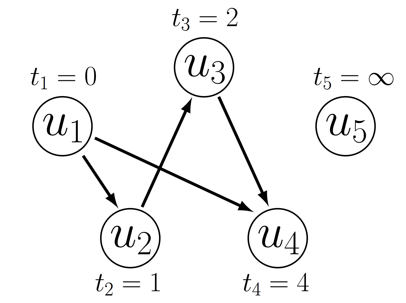
Figure 1: An illustrative example of one cascade.

Network structure and cascade generating process.

The model of Gomez-Rodriguez et al. (2011) assumes that the underlying network is composed of $p$ nodes and uses a non-negative diffusion matrix $A=\{\alpha_{ji}\}$ to parameterize the edges among them. The parameter $\alpha_{ji}$ measures the transmission rate from $j$ to $i$, where a larger $\alpha_{ji}$ means stronger connection from $j$ to $i$. The absence of $j\to i$ edge is denoted by $\alpha_{ji}=0$. For every node $i$, self infection is not considered and $\alpha_{ii}=0$. A cascade based on the model and network here is generated in the following way. At the beginning, at time $0$, one of the $p$ nodes is infected as a source node. When a node $j$ is infected, it samples a time at which it infects other uninfected nodes it is connected to. The transmission time $\tau_{ji}$ from node $j$ to $i$ follows a random distribution with a density $\ell(\tau;\alpha_{ji})$ for $\tau\geq 0$ (this density is called the transmission function/kernel). A node $i$ is infected the first time one of the nodes which can reach $i$ infects it. After being infected, node $i$ becomes a new source and begins to infect other nodes by following the same procedure and sampling the transmission times to other uninfected nodes that it can reach. An infected node continues to infect additional nodes after infecting one of its neighbor nodes.

The model assumes an observation window of length $T$ time units since the infection of the source node; nodes that are not infected until time $T$ are regarded as uninfected. We write $\ell(t_{i}\mid t_{j};\alpha_{ji})=\ell(t_{i}-t_{j};\alpha_{ji})$ to indicate the density that $i$ is infected by $j$ at time $t_{i}$ given that $j$ is infected at time $t_{j}$, parameterized by $\alpha_{ji}$. The transmission times of each infection are assumed to be independent, and a node remains infected in the whole process once it is infected.

Data.

In order to fit parameters of the model above, we assume that there are $n$ independent cascades denoted by the set $C^{n}=\{t^{1},\ldots,t^{n}\}$. A cascade $c$ is represented by $t^{c}$, which is a $p$-dimensional vector $t^{c}=(t_{1}^{c},\ldots,t_{p}^{c})$ indicating the time of infection of the $p$ nodes; $t_{i}^{c}\in[0,T^{c}]\bigcup\{\infty\}$ with $T^{c}$ being the observation window for the cascade $c$. Although not necessary, for notational simplicity we assume $T^{c}=T$ for all the cascades. For an infected node, only the first infected time is recorded even if it is infected by multiple neighbors. For the source node $i$, $t_{i}^{c}=0$, while node uninfected up to time $T$ we use the convention $t_{i}^{c}=\infty$. Moreover, the network structure is assumed to be static and not change while the $n$ different cascades are observed.

Likelihood function.

The likelihood function of an observed cascade $t$ is given by

$$\ell(t;A)=\prod\limits_{t_{i}\leq T}\prod\limits_{t_{m}>T}S(T\mid t_{i};\alpha_{im})\times\bigg{[}\prod\limits_{k:t_{k}<t_{i}}S(t_{i}\mid t_{k};\alpha_{ki})\sum_{j:t_{j}<t_{i}}H(t_{i}\mid t_{j};\alpha_{ji})\bigg{]},$$ (1)

where $S(t_{i}\mid t_{j};\alpha_{ji})=1-\int_{t_{j}}^{t_{i}}\ell(t-t_{j};\alpha_{ji})\,dt$ is the survival function and $H(t_{i}|t_{j};\alpha_{ji})=\ell(t_{i}-t_{j};\alpha_{ji})/S(t_{i}|t_{j};\alpha_{ji})$ is the hazard function (Gomez-Rodriguez et al., 2011). Note that the likelihood function consists of two probabilities. The first one is the probability that an uninfected node “survives” given its infected neighbors; the second one is the density that an infected node is infected at the specific observed time.

The transmission function affects the behavior of a cascade. Some commonly used transmission functions are exponential, Rayleigh, and power-law distributions (Gomez-Rodriguez et al., 2011). For exponential transmission, the diffusion rate reaches its maximum value at the beginning and then decreases exponentially. Because of this property, it can be used to model information diffusion on internet or a social network, since (breaking) news usually spread among people immediately, while with time a story gradually becomes unpopular. The exponential transmission function is given by

$$\ell(\tau;\alpha_{ji})=\alpha_{ji}\cdot\exp(-\alpha_{ji}\tau)$$ (2)

for $\tau\geq 0$ and $\ell(\tau;\alpha_{ji})=0$ otherwise. We then have $S(t+\tau\mid t;\alpha_{ji})=\exp(-\alpha_{ji}\tau)$ and $H(t+\tau\mid t;\alpha_{ji})=\alpha_{ji}$. As a different example, with the Rayleigh transmission function the diffusion rate is small at the beginning; it then rises to a peak and then drops. It can be used to model citation networks, since it usually takes some time to publish a new paper and cite the previous paper. New papers then gradually become known by researchers. The Rayleigh transmission function is given as

$$\ell(\tau;\alpha_{ji})=\alpha_{ji}\tau\cdot\exp\Big{(}-\frac{1}{2}\alpha_{ji}\tau^{2}\Big{)}$$

for $\tau\geq 0$ and $\ell(\tau;\alpha_{ji})=0$ otherwise. We then have $S(t+\tau\mid t;\alpha_{ji})=\exp(-\frac{1}{2}\alpha_{ji}\tau^{2})$ and $H(t+\tau\mid t;\alpha_{ji})=\alpha_{ji}\tau$. We will use these two transmission functions in Section 8 for modeling information diffusion on internet and in citation networks, respectively.

Optimization problem.

The unknown parameter is the diffusion matrix $A$, which can be estimated by maximizing the likelihood

$$\mathop{\text{minimize}}_{\alpha_{ji}}\quad-\frac{1}{n}\sum_{c\in C^{n}}\log\,{\ell(t^{c};A)}$$ (3)

$$\text{subject to}\quad\alpha_{ji}\geq 0,j\neq i.$$

A nice property of the above optimization program is that it can be further separated into $p$ independent subproblems involving individual columns of $A$. Specifically, the $i^{th}$ subproblem is to infer the incoming edges into the node $i$

$$\mathop{\text{minimize}}_{\alpha_{i}}\quad\,\phi(\alpha_{i})$$ (4)

$$\text{subject to}\,\,\,\,\,\alpha_{ji}\geq 0,j\neq i,$$

where the parameter $\alpha_{i}=\{\alpha_{ji}\mid j=1,\ldots,N,j\neq i\}$ denotes the $i^{th}$ column of $A$ and the objective function is

$$\phi(\alpha_{i})=-\frac{1}{n}\sum_{c\in C^{n}}\phi_{i}(t^{c};\alpha_{i}),$$

with $\phi_{i}(\cdot;\alpha_{i})$ denoting the likelihood function for one cascade. For example, for the exponential transmission function, we have

$$\phi_{i}({t};{\alpha}_{i})=\text{log}\Bigg{(}\sum_{j:t_{j}<t_{i}}\alpha_{ji}\Bigg{)}-\sum_{j:t_{j}<t_{i}}\alpha_{ji}(t_{i}-t_{j})$$ (5)

for an infected node, and

$$\phi_{i}({t};{\alpha}_{i})=-\sum_{j:t_{j}<T}\alpha_{ji}(T-t_{j})$$ (6)

for an uninfected node. See Gomez-Rodriguez et al. (2011) for more details.

The problem (4) is convex in $\alpha_{i}$ and can be solved by a standard gradient-based algorithm. The linear terms in (5) and (6) act as an $\ell_{1}$ penalty on the unknown parameter and automatically encourage sparse solutions. Nonetheless, adding an explicit $\ell_{1}$ penalty can further improve results. Gomez-Rodriguez et al. (2016) propose to solve the following regularized optimization problem

$$\mathop{\text{minimize}}_{\alpha_{i}}\quad\phi(\alpha_{i})+\lambda\|\alpha_{i}\|_{1}$$ (7)

$$\text{subject to}\quad\alpha_{ji}\geq 0,j\neq i,$$

using a proximal gradient algorithm (Parikh and Boyd, 2014).

2.2 Topic-sensitive Model

The basic model described above makes an unrealistic assumption that each cascade spreads based on the same diffusion matrix $A$. However, for example, posts on information technology usually spread much faster than those on economy and military. Du et al. (2013b) extend the basic model to incorporate this phenomena. Their topic-sensitive model assumes that there are in total $K$ topics, and each cascade can be represented as a topic vector in the canonical $K$-dimensional simplex, in which each component is the weight of a topic: ${m}^{c}:=(m_{1}^{c},...,m_{K}^{c})^{\top}$ with $\sum_{k}m_{k}^{c}=1$ and $m_{k}^{c}\in[0,1]$. Each topic $k$ is assumed to have its own diffusion matrix $A^{k}=\left\{\alpha_{ji}^{k}\right\}$, and the diffusion matrix of the cascade $A^{c}=\left\{\alpha_{ji}^{c}\right\}$ is the weighted sum of the $K$ matrices:

$$\alpha_{ji}^{c}=\sum_{k=1}^{K}\alpha_{ji}^{k}m_{k}^{c}.$$ (8)

In this way, the diffusion matrix $A^{c}$ can be different for different cascades. For each cascade $c$, the propagation model remains the same as the basic model described in the previous section, but with the diffusion matrix $A^{c}$ given in (8). The unknown parameters $A^{1},\ldots,A^{K}$ can be estimated by maximizing the regularized log-likelihood. Du et al. (2013b) use a group lasso type penalty and solve the following regularized optimization problem

$$\mathop{\text{minimize}}_{\alpha_{ji}^{k}}\quad-\frac{1}{n}\sum_{c\in C^{n}}\phi_{i}\Big{(}t^{c};\big{\{}\alpha_{ji}^{c}\big{\}}_{j=1}^{p}\Big{)}+\lambda\sum_{j}\|\alpha_{ji}\|_{2}$$ (9)

$$\text{subject to}\quad\alpha_{ji}^{c}=\sum_{k=1}^{K}\alpha_{ji}^{k}m_{k}^{c},$$

$$\qquad\qquad\quad\,\,\alpha_{ji}^{k}\geq 0,\,j\neq i,$$

with a proximal gradient based block coordinate descent algorithm.

3 An Influence-Receptivity Based Topic-sensitive Model

In this section we describe our proposed influence-receptivity model. Our motivation for proposing a new model for information diffusion stems from the observation that the two models discussed in Section 2 do not impose any structural assumptions on $A$ or $A^{k}$ other than nonnegativity and sparsity. However, in real world applications we observe node-topic interactions in the diffusion network. For example, different social media outlets usually focus on different topics, like information technology, economy or military. If the main focus of a media outlet is on information technology, then it is more likely to publish or cite news with that topic. Here the topics of interest of a media outlet impart the network structure. As another example, in a university, students may be interested in different academic subjects, may have different music preferences, or follow different sports. In this way it is expected that students who share the same or similar areas of interest may have much stronger connections. Here the areas of interest among students impart the structure to the diffusion network. Finally, in the context of epidemiology, people usually have different immune systems, and a disease such as flu, usually tends to infect some specific people, while leaving others uninfected. It is very likely that the infected people (by a specific disease) may have similar immune system, and therefore tend to become contagious together. Here the types of immune system among people impart the structure.

Taking this intuition into account, we build on the topic-sensitive diffusion model of Du et al. (2013b) by imposing a node-topic interaction. This interaction corresponds to the structural assumption on the cascade diffusion matrix $A^{c}$ for each cascade $c$. As before, a cascade $c$ is represented by its weight on $K$ topics ($K\ll p$): $m^{c}=(m_{1}^{c},m_{2}^{c},\ldots,m_{K}^{c})^{\top}$, with $\sum_{k}m_{k}^{c}=1$ and $m_{k}^{c}\in[0,1]$. Each node is parameterized by its “interest” in each of these $K$ topics as two $K$ dimensional (row) vectors. Stacking each of these two vectors together, the “interest” of all the $p$ nodes form two $p\times K$ dimensional matrices. To describe such structure, we propose two node-topic matrices $B_{1},B_{2}\in\mathbb{R}^{p\times K}$, where $B_{1}$ measures how much a node can infect others (the influence matrix) and $B_{2}$ measures how much a node can be infected by others (the receptivity matrix). We use $b_{ik}^{1}$ and $b_{ik}^{2}$ to denote the elements on $i^{th}$ row and $k^{th}$ column of $B_{1}$ and $B_{2}$, respectively. A large $b_{ik}^{1}$ means that node $i$ tends to infect others on topic $k$; while a large $b_{ik}^{2}$ means that node $i$ tends to be infected by others on topic $k$. These two matrices model the observation that, in general, the behaviors of infecting others and being infected by others are usually different. For example, suppose a media outlet $i$ has many experts in a topic $k$, then it will publish many authoritative articles on this topic. These articles are likely to be well-cited by others and therefore it has a large $b_{ik}^{1}$. However, its $b_{ik}^{2}$ may not be large, because $i$ has experts in topic $k$ and does not need to cite too many other news outlets on topic $k$. On the other hand, if a media outlet $i$ is only interested in topic $k$ but does not have many experts, then it will have a small $b_{ik}^{1}$ and a large $b_{ik}^{2}$.

For a specific cascade $c$ on topic $k$, there will be an edge $j\to i$ if and only if node $j$ tends to infect others on topic $k$ (large $b_{jk}^{1}$) and node $i$ tends to be infected by others on topic $k$ (large $b_{ik}^{2}$). For a cascade $c$ with the topic-weight $m^{c}$, the diffusion parameter $\alpha_{ji}^{c}$ is modeled as

$$\alpha_{ji}^{c}=\sum_{k=1}^{K}b_{jk}^{1}\cdot m_{k}^{c}\cdot b_{ik}^{2}.$$ (10)

The diffusion matrix for a cascade $c$ can be then represented as

$$A^{c}=B_{1}\cdot M^{c}\cdot B_{2}^{\top}=\sum_{k=1}^{K}m_{k}^{c}\cdot b_{k}^{1}{b_{k}^{2}}^{\top},$$ (11)

where $M^{c}={\rm diag}(m^{c})$ is a diagonal matrix representing the topic weight and $B_{j}=[b^{j}_{1},\ldots,b^{j}_{K}]$ with $b^{j}_{k}$ denoting the $k^{\text{th}}$ column of $B_{j}$, $j=1,2$. In a case where one does not consider self infection, we can modify the diffusion matrix for a cascade $c$ as

$$A^{c}=B_{1}M^{c}B_{2}^{\top}-\text{diag}(B_{1}M^{c}B_{2}^{\top}).$$

Under the model in (11), the matrix $M^{c}$ is known for each cascade $c\in C^{n}$, and the unknown parameters are $B_{1}$ and $B_{2}$ only. The topic weights can be obtained from a topic model, such as latent Dirichlet allocation (Blei et al., 2003), as long as we are given the text information of each cascade, for example, the main text in a website or abstract/keywords of a paper. The number of topics $K$ is user specified or can be estimated from data (Hsu and Poupart, 2016). The extension to a setting with an unknown topic distribution $M^{c}$ is discussed in Section 6.4.

With a known topic distribution $M^{c}$, our model has $2pK$ parameters. Compared to the basic model, which has $p^{2}$ parameters, and the topic-sensitive model, which has $p^{2}K$ parameters, we observe that our proposed model has much fewer parameters since, usually, we have $K\ll p$. Based on (11), our model can be viewed as a special case of the topic-sensitive model where each topic diffusion matrix $A^{k}$ is assumed to be of rank 1. A natural generalization of our model is to relax the constraint and consider topic diffusion matrices of higher rank, which would correspond to several influence and receptivity vectors affecting the diffusion together.

4 Estimation

In this section we develop an estimation procedure for parameters of the model described in the last section. In Section 4.1 and 4.2 we reparameterize the problem and introduce regularization terms in order to guarantee unique solution to estimation procedure. We then propose efficient algorithms to solve the regularized problem in Section 4.3.

4.1 Reparameterization

The negative log-likelihood function for our model is easily obtained by plugging the parametrization of a diffusion matrix in (11) into the original problem (3). Specifically, the objective function we would like to minimize is given by

$$f(B_{1},B_{2})=-\frac{1}{n}\sum_{c\in C^{n}}\log{\ell\big{(}t^{c};B_{1}M^{c}B_{2}^{\top}\big{)}}.$$ (12)

Unfortunately, this objective function is not separable in each column of $B_{1},B_{2}$, so we have to deal with entire matrices. Based on (11), recall that the diffusion matrix $A^{c}$ can be viewed as a weighted sum of $K$ rank-1 matrices. Let $\Theta_{k}=b_{k}^{1}{b_{k}^{2}}^{\top}$ and denote the collection of these rank-1 matrices as $\Theta=(\Theta_{1},\ldots,\Theta_{K})$. With some abuse of notation, the objective function $f(\cdot)$ in (12) can be rewritten as

$$f(\Theta)=f(\Theta_{1},\ldots,\Theta_{K})=-\frac{1}{n}\sum_{c\in C^{n}}\log{\ell\bigg{(}t^{c};\sum_{k=1}^{K}m_{k}^{c}\cdot\Theta_{k}\bigg{)}}.$$ (13)

Note that since $\log\ell(\cdot)$ is convex and $A^{c}$ is linear in $\Theta_{k}$, the objective function $f(\Theta)$ is convex in $\Theta$ when we ignore the rank-1 constraint on $\Theta_{k}$.

4.2 Parameter Estimation

To simplify the notation, we use $f(\cdot)$ to denote the objective function in (12) or (13), regardless of the parameterization as $B_{1},B_{2}$ or $\Theta$. From the parameterization $\Theta_{k}=b_{k}^{1}{b_{k}^{2}}^{\top}$, it is clear that if we multiply $b_{k}^{1}$ by a constant $\gamma$ and multiply $b_{k}^{2}$ by $1/\gamma$, the matrix $\Theta_{k}$ and the objective function (13) remain unchanged. In particular, we see that the problem is not identifiable if parameterized by $B_{1},B_{2}$. To solve this issues we add regularization.

A reasonable and straightforward choice of regularization is the $\ell_{1}$ norm regularization on $B_{1}$ and $B_{2}$. We define the following norm

$$g_{1}(B_{1},B_{2})=\big{\|}B_{1}+B_{2}\big{\|}_{1,1}\triangleq\sum_{i,k}b^{1}_{ik}+b^{2}_{ik}$$ (14)

and the regularized objective becomes

$$f_{1}(B_{1},B_{2})=-\frac{1}{n}\sum_{c\in C^{n}}\log{\ell\big{(}t^{c};B_{1}M^{c}B_{2}^{\top}\big{)}}+\lambda\cdot g_{1}(B_{1},B_{2}),$$ (15)

where $\lambda$ is a tuning parameter. With this regularization, if we focus on the $k^{\text{th}}$ column, then the term we would like to minimize is

$$\gamma\|b^{1}_{k}\|_{1}+\frac{1}{\gamma}\|b^{2}_{k}\|_{1}.$$ (16)

Clearly, in order to minimize (16) we should select $\gamma$ such that the two terms in (16) are equal. This means that, at the optimum, the column sums of $B_{1}$ and $B_{2}$ are equal. We therefore avoid the scaling issue by adding the $\ell_{1}$ norm penalty.

An alternative choice of the regularizer is motivated by the literature on matrix factorization (Jain et al., 2013; Tu et al., 2016; Park et al., 2018; Ge et al., 2016; Zhang et al., 2018). In a matrix factorization problem, the parameter matrix $X$ is assumed to be low-rank, which can be explicitly represented as $X=UV^{\top}$ where $X\in\mathbb{R}^{p\times p}$, $U,V\in\mathbb{R}^{p\times r}$, and $r$ is the rank of $X$. Similar to our problem, this formulation is also not identifiable. The solution is to add a regularization term $\|UU^{\top}-VV^{\top}\|_{F}^{2}$, which guarantees that the singular values of $U$ and $V$ are the same at the optimum (Zhu et al., 2017; Zhang et al., 2018; Park et al., 2018; Yu et al., 2020). Motivated by this approach, we consider the following regularization term

$$g_{2}(B_{1},B_{2})=\frac{1}{4}\cdot\sum_{k=1}^{K}\Big{(}\big{\|}b^{1}_{k}\big{\|}_{2}^{2}-\big{\|}b^{2}_{k}\big{\|}_{2}^{2}\Big{)}^{2},$$ (17)

which arises from viewing our problem as a matrix factorization problem with rank-1 matrices. The regularized objective function is therefore given by

$$f_{2}(B_{1},B_{2})=-\frac{1}{n}\sum_{c\in C^{n}}\log{\ell\big{(}t^{c};B_{1}M^{c}B_{2}^{\top}\big{)}}+\lambda\cdot g_{2}(B_{1},B_{2}).$$ (18)

Note that for this regularization penalty, at the minimum, we have that $g_{2}(B_{1},B_{2})=0$ and that the $\ell_{2}$-norm of the columns of $B_{1}$ and $B_{2}$ are equal. Furthermore, we can pick any positive regularization penalty $\lambda$.

In summary, both regularizers $g_{1}(\cdot)$ and $g_{2}(\cdot)$ force the columns of $B_{1}$ and $B_{2}$ to be balanced. At optimum the columns will have the same $\ell_{1}$ norm if $g_{1}$ is used and the same $\ell_{2}$ norm if $g_{2}$ is used. As a result, for each topic $k$, the total magnitudes of “influence” and “receptivity” are the same. In particular, a regularizer enforces the conservation law that the total amount of output should be equal to the total amount of input.

The $\ell_{1}$ norm regularizer induces a biased sparse solution. In contrast, the regularizer $g_{2}$ neither introduces bias nor encourages a sparse solution. Since in real world applications each node is usually interested in only a few topics, the two matrices $B_{1},B_{2}$ are assumed to be sparse, as we state in the next section. Taking this into account, if the regularizer $g_{2}$ is used, we need to threshold the estimator to obtain a sparse solution.

In conclusion, the optimization problem that we are going to solve is

$$\mathop{\text{minimize}}_{B_{1},B_{2}}\quad-\frac{1}{n}\sum_{c\in C^{n}}\log{\ell\big{(}t^{c};B_{1}M^{c}B_{2}^{\top}\big{)}}+\lambda\cdot g(B_{1},B_{2})$$ (19)

$$\text{subject to}\quad B_{1},B_{2}\geq 0,$$

where the regularization $g(\cdot)$ is either $g_{1}(\cdot)$, defined in (14), or $g_{2}(\cdot)$, defined in (17).

4.3 Optimization Algorithm

While the optimization program (3) is convex in the diffusion matrix $A$, the proposed problem (19) is nonconvex in $B_{1},B_{2}$. Our model for a diffusion matrix (11) is bilinear and, as a result, the problem (19) is a biconvex problem in $B_{1}$ and $B_{2}$, that is, the problem is convex in $B_{1}$ and $B_{2}$, but not jointly convex. Gorski et al. (2007) provide a survey of methods for minimizing biconvex functions. In general, there are no efficient algorithms for finding the global minimum of a biconvex problem. Floudas (2000) propose a global optimization algorithm, which alternately solves primal and relaxed dual problem. This algorithm is guaranteed to find the global minimum, but the time complexity is usually exponential. For our problem, we choose to develop a gradient-based algorithm. For the regularizer $g_{1}$, since the $\ell_{1}$ norm is non-smooth, we develop a proximal gradient descent algorithm (Parikh and Boyd, 2014); for the regularizer $g_{2}$, we use an iterative hard thresholding algorithm (Yu et al., 2020).

Algorithm 1 Proximal gradient descent for (19) with regularizer $g_{1}(\cdot)$

  Initialize $B_{1}^{(0)}$, $B_{2}^{(0)}$

  while $tolerance>\epsilon$ do

     $B_{1}^{(t+1)}=\Big{[}B_{1}^{(t)}-\eta\nabla_{B_{1}}f\big{(}B_{1}^{(t)},B_{2}^{(t)}\big{)}-\lambda\eta\Big{]}_{+}$

     $B_{2}^{(t+1)}=\Big{[}B_{2}^{(t)}-\eta\nabla_{B_{2}}f\big{(}B_{1}^{(t)},B_{2}^{(t)}\big{)}-\lambda\eta\Big{]}_{+}$

  end while

Algorithm 2 Gradient descent with hard thresholding for (19) with regularizer $g_{2}(\cdot)$

  Initialize $B_{1}^{(0)}$, $B_{2}^{(0)}$

  while $tolerance>\epsilon$ do

     $B_{1}^{(t+0.5)}=\Big{[}B_{1}^{(t)}-\eta\cdot\nabla_{B_{1}}f\big{(}B_{1}^{(t)},B_{2}^{(t)}\big{)}-\eta\cdot\nabla_{B_{1}}g_{2}\big{(}B_{1}^{(t)},B_{2}^{(t)}\big{)}\Big{]}_{+}$

     $B_{1}^{(t+1)}=\text{Hard}\big{(}B_{1}^{(t+0.5)},s\big{)}$

     $B_{2}^{(t+0.5)}=\Big{[}B_{2}^{(t)}-\eta\cdot\nabla_{B_{2}}f\big{(}B_{1}^{(t)},B_{2}^{(t)}\big{)}-\eta\cdot\nabla_{B_{2}}g_{2}\big{(}B_{1}^{(t)},B_{2}^{(t)}\big{)}\Big{]}_{+}$

     $B_{2}^{(t+1)}=\text{Hard}\big{(}B_{2}^{(t+0.5)},s\big{)}$

  end while

Since the optimization problem (19) is nonconvex, we need to carefully initialize the iterates $B_{1}^{(0)},B_{2}^{(0)}$ for both algorithms. We find the initial iterates by minimizing the objective function $f(\Theta)$, defined in (13), without the rank-1 constraint. As discussed earlier, the objective function $f(\Theta)$ is convex in $\Theta$ and can be minimized by, for example, the gradient descent algorithm. After obtaining the minimizer $\widehat{\Theta}=(\widehat{\Theta}_{1},\ldots,\widehat{\Theta}_{K})$, we find the best rank-1 approximation of each $\widehat{\Theta}_{k}$. According to the Eckart-Young-Mirsky theorem, the best rank-1 approximation is obtained by the singular value decomposition (SVD) by keeping the largest singular value and corresponding singular vectors. Specifically, suppose the leading term of SVD for $\widehat{\Theta}_{k}$ is denoted as $\sigma_{k}u_{k}v_{k}^{\top}$ for each $k$, then the initial values are given by $B_{1}^{(0)}=\text{Hard}\big{(}[u_{1}\sigma_{1}^{1/2},\ldots,u_{K}\sigma_{K}^{1/2}],s\big{)}$ and $B_{2}^{(0)}=\text{Hard}\big{(}[v_{1}\sigma_{1}^{1/2},\ldots,v_{K}\sigma_{K}^{1/2}],s\big{)}$. Starting from $B_{1}^{(0)}$, $B_{2}^{(0)}$, we apply one of the two gradient-based algorithms described in Algorithm 1 and Algorithm 2, until convergence to a pre-specified tolerance level $\epsilon$ is reached. The gradient $\nabla_{B}f(B_{1},B_{2})$ can be calculated by the chain rule. The specific form depends on the transmission function used. In practice, the tuning parameters $\lambda$ and $s$ can be selected by cross-validation. Based on our experience, both algorithms provide good estimators for $B_{1}$ and $B_{2}$. To further accelerate the algorithm one can use the stochastic gradient descent algorithm.

5 Theoretical Results

In this section we establish main theoretical results. Since the objective function is nonconvex in $B_{1},B_{2}$, proving theoretical result based on the $\ell_{1}$ norm penalization is not straightforward. For example, the usual analysis applied to nonconvex M-estimators (Loh and Wainwright, 2015) assumes a condition called restricted strong convexity, which does not apply to our model. Therefore, to make headway on our problem, we focus on the optimization problem with the regularizer $g_{2}$ and leverage tools that have been used in analyzing matrix factorization problems (Jain et al., 2013; Tu et al., 2016; Park et al., 2018; Ge et al., 2016; Zhang et al., 2018; Na et al., 2019, 2020). Compared to these works which focus on recovering one rank-$K$ matrix, our goal is to recover $K$ rank-1 matrices.

Let $B_{1}^{*},B_{2}^{*}$ denote the true influence and receptivity matrices; the corresponding rank-1 matrices are given by $\Theta_{k}^{*}={b^{1}_{k}}^{*}{b^{2}_{k}}^{*\top}$, for each topic $k$. We start by stating assumptions under which the theory is developed. The first assumption states that the parameter matrices are sparse.

Assumption 1

Each column of the true influence and receptivity matrices are assumed to be sparse with $\|b_{k}^{1*}\|_{0}=\|b_{k}^{2*}\|_{0}=s^{*}$, where $\|b\|_{0}=\big{|}j:b_{j}\neq 0\big{|}$ denotes the number of nonzero components of a vector.

The above assumption can be generalized in a straightforward way to allow different columns to have different levels of sparsity.

The next assumption imposes regularity conditions on the Hessian matrix of the objective function. First, we recall the Hessian matrix corresponding to the objective function $\phi(\alpha)$ in (4) for the basic cascade model. For a cascade $c$, the Hessian matrix is given by

$$\mathcal{Q}(\alpha)=D(\alpha)+X(t^{c};\alpha)\cdot X(t^{c};\alpha)^{\top},$$ (20)

where $D(\alpha)$ is a diagonal matrix,

$$X(t^{c};\alpha)=h(t^{c};\alpha)^{-1}\nabla_{\alpha}h(t^{c};\alpha),$$

with

$$h(t;\alpha)=\begin{cases}\sum_{j:t_{j}<t_{i}}H(t_{i}|t_{j};\alpha_{ji})&\mbox{if }t_{i}<T,\\ 0&\mbox{otherwise},\end{cases}$$

and $H(t_{i}|t_{j};\alpha_{ji})$ is the hazard function defined in Section 2.1. Recalling that $\alpha\in\mathbb{R}^{p}$ denotes the $i^{\text{th}}$ column of $A$, we have that $\mathcal{Q}(\alpha)\in\mathbb{R}^{p\times p}$. Both $D(\alpha)$ and $X(t^{c};\alpha)$ are simple for the common transmission functions. For example, for exponential transmission, we have that $D(\alpha)=0$ is the all zero matrix and

$$\big{[}X(t^{c};\alpha)\big{]}_{j}=\begin{cases}\Big{(}\sum_{\ell:t_{\ell}<t_{i}}\alpha_{\ell i}\Big{)}^{-1}&\mbox{if }t_{j}<t_{i}\\ 0&\mbox{otherwise.}\end{cases}$$ (21)

See Gomez-Rodriguez et al. (2016) for more details.

Let $[\Theta_{k}]_{i}\in\mathbb{R}^{p}$ denote the $i^{\text{th}}$ column of $\Theta_{k}$ and let $\Theta^{[i]}=\Big{[}[\Theta_{1}]_{i},[\Theta_{2}]_{i},\ldots,[\Theta_{K}]_{i}\Big{]}\in\mathbb{R}^{p\times K}$ be the collection of $K$ such columns. Since $A^{c}=\sum_{k}m_{k}^{c}\cdot\Theta_{k}$, we have that the $i^{\text{th}}$ column of $A^{c}$ is a linear combination of $\Theta^{[i]}$. Therefore, the Hessian matrix of $f(\Theta)$ with respect to $\Theta^{[i]}$ is a quadratic form of the Hessian matrices defined in (20). For a specific cascade $c$, denote the transformation matrix as

$$P^{c}=\begin{bmatrix}m_{1}^{c}\cdot I_{p}&m_{2}^{c}\cdot I_{p}&\ldots&m_{K}^{c}\cdot I_{p}\end{bmatrix}\in\mathbb{R}^{p\times pK}.$$ (22)

Then we have $\alpha_{i}^{c}=P^{c}\cdot\Theta^{[i]}$, where $\alpha_{i}^{c}$ denotes the $i^{\text{th}}$ column of $A^{c}$. Using the chain rule, we obtain that the Hessian matrix of $f(\Theta)$ with respect to $\Theta^{[i]}$ for one specific cascade $c$ is given by

$$H^{c}\big{(}\Theta^{[i]}\big{)}={P^{c}}^{\top}\cdot\mathcal{Q}(\alpha_{i}^{c})\cdot P^{c}\in\mathbb{R}^{pK\times pK}.$$ (23)

The Hessian matrix of the objective function $f(\Theta)$ with respect to $\Theta^{[i]}$ is now given as

$$H(\Theta^{[i]})=\frac{1}{n}\sum_{c}H^{c}(\Theta^{[i]}).$$

We make the following assumption on the Hessian matrix.

Assumption 2

There exist constants $\mu,L>0$, so that $\mu\cdot I_{pK}\preceq H(\Theta^{[i]})\preceq L\cdot I_{pK}$ hold uniformly for any $i\in\{1,\ldots,p\}$.

The optimization problem (3), used to find the diffusion matrix $A$ for the basic cascade model, is separable across columns of $A$ as shown in (4). Similarly, the objective function $f(\Theta)$ is separable across $\Theta^{[i]}$, if we ignore the rank-1 constraint. As a result, the Hessian matrix of $f(\Theta)$ with respect to $\Theta$, is (after an appropriate permutation of rows and columns) a block diagonal matrix in $\mathbb{R}^{p^{2}K\times p^{2}K}$ with each block given by $H(\Theta^{[i]})\in\mathbb{R}^{p\times p}$. Therefore, Assumption 2 ensures that $f(\Theta)$ is strongly convex and smooth in $\Theta$.

The upper bound in Assumption 2 is easy to satisfy. The lower bound ensures that the problem is identifiable. The Hessian matrix depends in a non-trivial way on the network structure, diffusion process, and the topic distributions. Without the influence-receptivity structure, Gomez-Rodriguez et al. (2016) establish conditions for the basic cascade model under which we can recover the network structure consistently from the observed cascades. The conditions require that the behavior of connected nodes are reasonably similar among the cascades, but not deterministically related; and also that connected nodes should get infected together more often than non-connected nodes. Assumption 2 is also related to the setting in Yu et al. (2019), who consider the squared loss, where the condition ensures that the topic distribution among the $n$ cascades is not too highly correlated, since otherwise we cannot distinguish them. In our setting, Assumption 2 is a combination of the two cases: we require that the network structure, diffusion process, and the topic distributions interact in a way to make the problem is identifiable. We refer the readers to Gomez-Rodriguez et al. (2016) and Yu et al. (2019) for additional discussions.

Subspace distance.

Since the factorization of $\Theta_{k}$ as $\Theta_{k}={b^{1}_{k}}{b^{2}_{k}}^{\top}$ is not unique, as discussed earlier, we will measure convergence of algorithms using the subspace distance. Define the set of $r$-dimensional orthogonal matrices as

$$\mathcal{O}(r)=\{O\in\mathbb{R}^{r\times r}:O^{\top}O=OO^{\top}=I_{r}\}.$$

Suppose $X^{*}\in\mathbb{R}^{p\times p}$ is a rank-$r$ matrix that can be decomposed as $X^{*}={U^{*}}{V^{*}}^{\top}$ with $U^{*},V^{*}\in\mathbb{R}^{p\times r}$  and $\sigma_{i}(U^{*})=\sigma_{i}(V^{*})$ where $\sigma_{i}(U)$ denotes the $i^{\rm{th}}$ singular value of $U$. Let $X=UV^{\top}$ be an estimator of $X^{*}$. The subspace distance between $X$ and $X^{*}$ is measured as

$$\min_{O\in\mathcal{O}(r)}\Big{\{}\|U-U^{*}O\|_{F}^{2}+\|V-V^{*}O\|_{F}^{2}\Big{\}}.$$ (24)

The above formula measures the distance between matrices up to an orthogonal rotation. For our problem, the matrices $\Theta_{k}$ are constrained to be rank-1, and the only possible rotation is given by $o=\pm 1$. Moreover, since $B_{1},B_{2}\geq 0$ are nonnegative, the negative rotation is eliminated. As a result, the subspace distance for our problem reduces to the usual Euclidean distance. Let $B=[B_{1},B_{2}]$ and $B^{*}=[B_{1}^{*},B_{2}^{*}]$, then the “subspace distance” between $B$ and $B^{*}$ is defined as

$$d^{2}(B,B^{*})=\min_{o_{k}\in\{\pm 1\}}\sum_{k=1}^{K}\big{\|}b_{k}^{1}-{b_{k}^{1}}^{*}o_{k}\big{\|}_{2}^{2}+\big{\|}b_{k}^{2}-{b_{k}^{2}}^{*}o_{k}\big{\|}_{2}^{2}=\big{\|}B_{1}-B_{1}^{*}\big{\|}_{F}^{2}+\big{\|}B_{2}-B_{2}^{*}\big{\|}_{F}^{2}.$$ (25)

Statistical error.

The notion of the statistical error measures how good our estimator can be. In a statistical estimation problem with noisy observations, even the best estimator can only be an approximation to the true parameter. The statistical error measures how well the best estimator estimates the true unknown parameter. For a general statistical estimation problem, the statistical error is usually defined as the norm of the gradient of the objective function evaluated at the true parameter. For our problem, since we have rank-1 and sparsity constraints, we define the statistical error as

$$e_{\text{stat}}=\sup_{\Delta\in\Omega(s)}\,\big{\langle}\nabla_{\Theta}f(\Theta^{*}),\Delta\big{\rangle},$$ (26)

where the set $\Omega(s)$ is defined as

$$\Omega(s)=\big{\{}\Delta:\Delta=[\Delta_{1},\ldots,\Delta_{K}],\Delta_{k}\in\mathbb{R}^{p\times p},{\rm rank}(\Delta_{k})=2,\|\Delta_{k}\|_{0}=2s^{2},\|\Delta\|_{F}=1\big{\}}.$$ (27)

The statistical error depends on the network structure, diffusion process, and the topic distributions, and it scales as $n^{-1/2}$ with the sample size.

With these preliminaries, we are ready to state the main theoretical results for our proposed algorithm. Our first result quantifies the accuracy of the initialization step. Let

$$\widehat{\Theta}=\arg\min_{\Theta}\ f(\Theta)$$

be the unconstrained minimizer of $f(\Theta)$.

Theorem 3

Suppose Assumption 2 is satisfied, and we set $s=c\cdot s^{*}$ in Algorithm 2 for some constant $c>1$. We have

$$\big{\|}\widehat{\Theta}-\Theta^{*}\big{\|}_{F}^{2}\leq\frac{2}{\mu}\big{\|}\nabla f(\Theta^{*})\big{\|}_{F}.$$ (28)

Furthermore,

$$d^{2}\big{(}B^{(0)},B^{*}\big{)}\leq\frac{80\xi^{2}K\big{\|}\nabla f(\Theta^{*})\big{\|}_{F}^{2}}{\mu^{2}\sigma^{*}},$$ (29)

where $\xi$ is defined as $\xi^{2}=1+\frac{2}{\sqrt{c-1}}$ and $\sigma^{*}=\min_{k}\|\Theta_{k}^{*}\|_{2}$.

The upper bound obtained in (28) and (29) can be viewed as a statistical error for the problem without rank-1 constraints. As a statistical error, the upper bound naturally scales with the sample size as $n^{-1/2}$. With a large enough sample size, the initial point will be within the radius of convergence to the true parameter such that

$$d^{2}\big{(}B^{(0)},B^{*}\big{)}\leq{\frac{1}{4}\gamma\sigma^{*}}\cdot\min\Big{\{}1,\frac{1}{4(\mu+L)}\Big{\}},$$ (30)

where $\gamma=\min\{1,\mu L/(\mu+L)\}$ . This enables us to prove the following result.

Theorem 4

Suppose Assumptions 1 and 2 are satisfied. Furthermore, suppose the sample size $n$ is large enough so that (30) holds and

$$e_{\rm stat}^{2}\leq\frac{1-\beta}{3\eta K\xi^{2}}\cdot\frac{\mu L}{\mu+L}\cdot{\frac{1}{4}\gamma\sigma^{*}}\cdot\min\Big{\{}1,\frac{1}{4(\mu+L)}\Big{\}}.$$

Then the iterates obtained by Algorithm 2, with $s=c\cdot s^{*}$, $c>1$, and the step size

$$\eta\leq\frac{1}{8\|B^{(0)}\|_{2}^{2}}\cdot\min\Big{\{}\frac{K}{2(\mu+L)},1\Big{\}},$$ (31)

satisfy

$$d^{2}\Big{(}B^{(T)},B^{*}\Big{)}\leq\beta^{T}\cdot d^{2}\Big{(}B^{(0)},B^{*}\Big{)}+\frac{C}{1-\beta}\cdot e^{2}_{\rm{stat}},$$ (32)

where $\beta<1$ and $C$ is a constant.

Theorem 4 establishes convergence of iterates produced by properly initialized Algorithm 2. The first term in (32) corresponds to the optimization error, which decreases exponentially with the number of iterations, while the second term corresponds to the unavoidable statistical error. In particular, Theorem 4 shows linear convergence of the iterates up to statistical error, which depends on the network structure, diffusion process, and the topic distributions. Note that the condition on $e_{\rm stat}$ is not stringent, since in the case that it is not satisfied, then already the initial point $B^{(0)}$ is accurate enough.

Proofs of Theorem 3 and 4 are given in Appendix.

6 Some Variants and Extensions

In this section we discuss several variants and application specific extensions of the proposed model. Section 6.1 considers the extension where in addition to the influence and receptivity to topics, information propagation is further regulated by a friendship network. Section 6.2 discusses how we can use the $B_{1}$ and $B_{2}$ matrices to estimate the topic distribution of a new cascade for which we do not have the topic distribution apriori. Section 6.3 discusses how estimated matrices $B_{1}$ and $B_{2}$ can serve as embedding of the nodes. Finally, in Section 6.4 we consider estimation of $B_{1},B_{2}$ in the setting where the topic distributions of cascades are unknown.

6.1 Cascades Regulated by Friendship Networks

We have used news and media outlets as our running example so far and have assumed that each node can influence any other node. However, in social networks, a user can only see the news or tweets published by their friends or those she chooses to follow. If two users do not know each other, then even if they are interested in similar topics, they still cannot “infect” each others. Considering this we can modify our model in the following way:

$$A^{c}=B_{1}M^{c}B_{2}^{\top}\otimes F,$$ (33)

where $\otimes$ denotes element-wise multiplication. $F\in\{0,1\}^{p\times p}$ is a known matrix indicating whether two nodes are “friends” ($f_{ji}=1$) or not ($f_{ji}=0$). The modified optimization problem is a straightforward extension of (19) obtained by replacing the expression for $A^{c}$ with the new model (33). The only thing that changes in Algorithms 1 and 2 is the gradient calculation.

As a further modification, we can allow for numeric values in $F$. Here we again have $f_{ji}=0$ if node $j$ and $i$ are not friends; when node $j$ and $i$ are friends, the value $f_{ji}>0$ measures how strong the friendship is. A larger value means a stronger friendship, and hence node $j$ could infect node $i$ in a shorter period of time. Under this setting, we assume knowledge of whether $f_{ji}$ is 0 or not, but not the actual value of $f_{ji}$ when it is non-zero. This modification is useful in dealing with information diffusion over a social network where we know whether two nodes are friends or not, but we do not know how strong the friendship is. We then have to estimate $B=[B_{1},B_{2}]$ and $F$ jointly, resulting in a more difficult optimization problem. A practical estimation procedure is to alternately optimize $B$ and $F$. With a fixed $F$, the optimization problem for $B$ can be solved using Algorithm 1 or 2, except for an additional element-wise multiplication with $F$ when calculating gradient. With a fixed $B$, the optimization problem in $F$ is convex and, therefore, can be solved by any gradient-based iterative algorithm.

6.2 Estimating Topic Distribution $m^{c}$

Up to now we have assumed that each topic distribution $M^{c}={\rm diag}(m^{c})$ is known. However, once $B_{1},B_{2}$ have been estimated, we can use them to classify a new cascade $c$ by recovering its topic-weight vector $m^{c}$. For example, if an unknown disease becomes prevalent among people, then we may be able to determine the type of this new disease and identify the vulnerable population of nodes. Moreover, with estimated $B_{1}$ and $B_{2}$, we can recalculate the topic distribution of all the cascades used to fit the model. By comparing the estimated distribution with the topic distribution of the cascades we can find the ones where the two topic distributions differ a lot. These cascades are potentially “outliers” or have abnormal propagation behavior and should be further investigated.

The maximum likelihood optimization problem for estimating the topic distribution $m^{c}$ is:

$$\mathop{\text{minimize}}_{m_{k}^{c}}\quad-\log{\ell\big{(}t^{c};B_{1}M^{c}B_{2}^{\top}\big{)}}$$ (34)

$$\text{subject to}\quad\sum_{k}m_{k}^{c}=1,$$

$$\,\,\,\quad\qquad\qquad 0\leq m_{k}^{c}\leq 1.$$

This problem is easier to solve than (19) since $A^{c}=B_{1}M^{c}B_{2}^{\top}$ is linear in $M^{c}$ and therefore the problem is convex in $M^{c}$. The constraint $\sum_{k}m^{c}_{k}=1$ and $0\leq m_{k}^{c}\leq 1$ can be incorporated in a projected gradient descent method, where in each iteration we apply gradient descent update on $M^{c}$ and project it to the simplex.

6.3 Interpreting Node-topic Matrices $B_{1}$ and $B_{2}$

While throughout the paper we have used the diffusion of news as a running example, our model and the notion of “topic” is much more broadly applicable. As discussed before it can represent features capturing susceptibility to diseases, as well as, geographic position, nationality, etc. In addition to the ability to forecast future information cascades, the influence-receptivity matrices $B_{1}$ and $B_{2}$ can also find other uses. For example, we can use the rows of $B_{2}$ to learn about the interests of users and for customer segmentation. In epidemiology, we can learn about the vulnerability of population to different diseases, and allocate resources accordingly.

The rows of $B_{1},B_{2}$ act as a natural embedding of users in $\mathbb{R}^{2K}$ and thus define a similarity metric, which can be used to cluster the nodes or build recommender systems. In Section 8 illustrate how to use this embedding to cluster and visualize nodes. The influence-receptivity structure is thus naturally related to graph embedding. See Cai et al. (2018) for a recent comprehensive survey of graph embedding. As a closely related work in graph embedding literature, Chen et al. (2017) propose a model which also embeds nodes into $\mathbb{R}^{2K}$. Compared to their model, our model allows for interaction of embedding (influence and receptivity) vectors and the topic information, resulting in more interpretable topics. Moreover, our model has flexibility to choose the transmission function based on different applications and comes with theoretical results on convergence rate and error analysis. For example, as will be shown in Section 8, for information propagation on the internet (for example, media outlets citing articles, Facebook and Twitter users sharing posts), we can choose the exponential transmission function; for the citation network, the Raleigh transmission function is a more appropriate choice.

6.4 When Topic Distribution is Unknown

Throughout the paper we assume that the topic distribution $M^{c}$ is known for each cascade. For example, the topic distribution can be calculated by Topic Modeling (Blei et al., 2003) with the text information of each cascade. Alternatively it can come from the knowledge of domain experts. However, in many applications domain experts or textual information may be unavailable. Even if such resources are available, the topic distribution obtained from Topic Modeling may be inaccurate or intractable in practice. In this case we must learn the topic distribution and the influence-receptivity structure together. For this problem, our observations constitute of the timestamps for each cascade as usual, and the variables to be optimized are $B=[B_{1},B_{2}]$ and $M^{c}$ for each cascade $c$. A practical algorithm is to alternately optimize on $B$ and $M^{c}$—with a fixed $M^{c}$, we follow Algorithm 1 or 2 to update $B$; with a fixed $B$, we follow (LABEL:eq:optimize_on_M) to update $M^{c}$ on each $c$. The two procedures are repeated until convergence.

Theoretical analysis of this alternating minimization algorithm under the log-likelihood in (1) is beyond the scope of the paper. For a simpler objective functions, such as the $\ell_{2}$ loss, the theoretical analysis is tractable and the output of the alternating minimization algorithm (the estimated $B$ and $M$) can be shown to converge to the true value up to the statistical error in both $B$ and $M$. Specifically, we denote $M^{*}$ as the true topic distribution and $f(\Theta,M)$ as the loss function defined in (13). Denote the statistical error defined in (26) as $e_{\text{stat},B}$ and similarly define the statistical error on the topic distribution $M$ as

$$e_{\text{stat},M}^{2} =\sum_{c\in C^{n}}\sum_{k=1}^{K}\Big{[}\nabla_{m^{c}_{k}}\,f(\Theta^{*},M^{*})\Big{]}^{2}.$$ (35)

Denote $B^{[t]}$ and $M^{[t]}$ as the output of the alternating minimization algorithm at iteration $t$. Under some additional mild assumptions, after one iterate of the alternating minimization algorithm we have the contraction on $B$ as

$$d^{2}\big{(}B^{[t+1]},B^{*}\big{)}\leq C_{1}\cdot e^{2}_{{\rm{stat}},B}+\beta_{1}\cdot d^{2}\big{(}M^{[t]},M^{*}\big{)},$$ (36)

for some constant $C_{1}$ and $\beta_{1}<1$. Similarly, after one iterate of the alternating minimization algorithm we have the contraction on $M$ as

$$d^{2}\big{(}M^{[t+1]},M^{*}\big{)}\leq C_{2}\cdot e_{{\rm{stat}},M}^{2}+\beta_{2}\cdot d^{2}\big{(}B^{[t]},B^{*}\big{)},$$ (37)

for some constant $C_{2}$ and $\beta_{2}<1$. Combining these two inequalities, after $T$ iterations of the alternative minimization algorithm we get

$$d^{2}\big{(}B^{[T]},B^{*}\big{)} +d^{2}\big{(}M^{[T]},M^{*}\big{)}\leq C_{0}(e_{{\rm stat},M}^{2}+e_{{\rm stat},B}^{2})+\beta_{0}^{T}\Big{[}d^{2}\big{(}B^{[0]},B^{*}\big{)}+d^{2}\big{(}M^{[0]},M^{*}\big{)}\Big{]},$$ (38)

for some constant $\beta_{0}=\max\{\beta_{1},\beta_{2}\}<1$. This shows that the iterates of the alternating minimization algorithm converge linearly to the true values up to statistical error. We refer the readers to Section 5 of Yu et al. (2019) for more details.

7 Synthetic Data Sets

In this section we demonstrate the effectiveness of our model on synthetic data sets. Since several existing algorithms are based on the $\ell_{1}$ norm regularization, for fair comparison, we focus on our proposed Algorithm 1.

7.1 Estimation Accuracy

We first evaluate our model on a synthetic data set and compare the predictive power of the estimated model with that of Netrate and TopicCascade. In simulation we set $p=200$ nodes, $K=10$ topics. We generate the true matrices $B_{1}$ and $B_{2}$ row by row. For each row, we randomly pick 2-3 topics and assign a random number Unif$(0.8,1.8)\cdot\zeta$, where $\zeta=3$ with probability 0.3 and $\zeta=1$ with probability 0.7. We make 30% of the values 3 times larger to capture the large variability in interests. All other values are set to be 0 and we scale $B_{1}$ and $B_{2}$ to have the same column sum. To generate cascades, we randomly choose a node $j$ as the source. The $j^{th}$ row of $B_{1}$ describes the “topic distribution” of node $j$ on infecting others. Therefore we sample a $K$ dimensional topic distribution $m^{c}$ from Dir($b^{1}_{j,:}$), where $b^{1}_{j,:}$ is the $j^{th}$ row of $B_{1}$ and Dir($\cdot$) is Dirichlet distribution, which is widely used to generate weights (Du et al., 2013b; He et al., 2019; Glynn et al., 2019; He and Hahn, 2020). According to our model (11), the diffusion matrix of this cascade is $A^{c}=B_{1}M^{c}B_{2}^{\top}$. The rest of the cascade propagation follows the description in Section 2.1. For experiments we use exponential transmission function as in (2). The diffusion process continues until either the overall time exceeds the observation window $T=1$, or there are no nodes reachable from the currently infected nodes. We record the first infection time for each node.

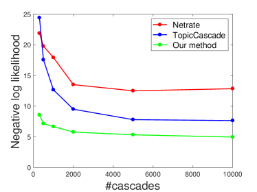
(a) Negative log-likelihood on test data set

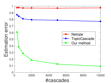
(b) Estimation error

Figure 2: Comparison of our method with Netrate and TopicCascade.

We vary the number of cascades $n\in\{300,500,1000,2000,5000,10000\}$. For all three models, we fit the model on a training data set and choose the regularization parameter $\lambda$ on a validation data set. Each setting of $n$ is repeated 5 times and we report the average value. We consider two metrics to compare our model with NetRate (Gomez-Rodriguez et al., 2011) and TopicCascade (Du et al., 2013b):

(1) We generate independent $n=5000$ test data and calculate negative log-likelihood function on test data for the three models. A good model should be able to generalize well and hence should have small negative log-likelihood. From Figure 2(a) we see that, when the sample size is small, both Netrate and TopicCascade have large negative log-likelihood on test data set; while our model generalizes much better. When sample size increases, NetRate still has large negative log-likelihood because it fails to consider the topic structure; TopicCascade behaves more and more closer to our model, which is as expected, since our model is a special case of the the topic-sensitive model. However, our model requires substantially fewer parameters.

(2) We calculate the true diffusion matrix $A^{k}$ for each topic $k$ based on our model: $A^{k}=B_{1}M_{(k)}B_{2}^{\top}$ where $M_{(k)}$ is diagonal matrix with 0 on all diagonal elements but 1 on location $k$. We also generate the estimated $\widehat{A}^{k}$ from the three models as follows: for our model we use the estimated $\widehat{B}_{1}$ and $\widehat{B}_{2}$; for TopicCascade model the $\widehat{A}^{k}$ is estimated directly as a parameter of the mode; for Netrate we use the estimated $\widehat{A}$ as the common topic diffusion matrix for each topic $k$. Finally, we compare the estimation error of the three models: ${\rm error}=\frac{1}{K}\sum_{k=1}^{K}\frac{\|\widehat{A}^{k}-A^{k}\|}{\|A^{k}\|}$. From Figure 2(b) we see that both Netrate and TopicCascade have large estimation error even if we have many samples; while our model has much smaller estimation error.

Dense graph.

We evaluate the performance of our method on a denser graph. When generating each row of $B_{1},B_{2}$, we randomly pick 5-6 topics instead of 2-3. This change makes infections more frequent. For many of the cascades, almost all the nodes are infected. Since this phenomenon is not common in practice, we shrink $B_{1}$ and $B_{2}$ by half, and reduce the maximum observation time $T$ by half to make sure that infection happens across about 30% of the nodes as before. The comparison of our method with Netrate and TopicCascade with dense graph is shown in Figure 3. We see that the pattern is similar to the previous experiments.

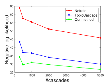
(a) Negative log-likelihood on test data set

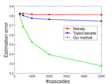
(b) Estimation error

Figure 3: Comparison of our method with Netrate and TopicCascade on a dense graph.

Kronecker graph.

We generate $B_{1}$ and $B_{2}$ according to the Kronecker graph (Leskovec et al., 2010). We consider two choices of parameters for generating the Kronecker graph that resemble the real world networks: the first one is [0.8 0.6; 0.5 0.3], and the second one is [0.7 0.7; 0.6 0.4]. For each choice of parameters, we follow the procedure in Leskovec et al. (2010) to generate a network with $2^{11}=2048$ nodes. Denote this adjacency matrix as $A^{\text{Kron}}\in\mathbb{R}^{2048\times 2048}$. Matrices $B_{1},B_{2}\in\mathbb{R}^{2048\times 10}$ are obtained from a non-negative matrix factorization of $A^{\text{Kron}}$, $A^{\text{Kron}}\approx B_{1}B_{2}^{\top}$. This corresponds to $K=10$. We randomly select $p=200$ nodes and discard others. This gives $B_{1},B_{2}\in\mathbb{R}^{200\times 10}$. Finally, we zero out small values in $B_{1}$ and $B_{2}$, scale them and treat them as the true parameters so that the percentage of infections behaves similar as the previous experiments. Figure 4 and 5 show the comparison on Kronecker graph. Once again, our method has the best performance.

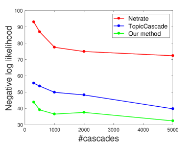
(a) Negative log-likelihood on test data set

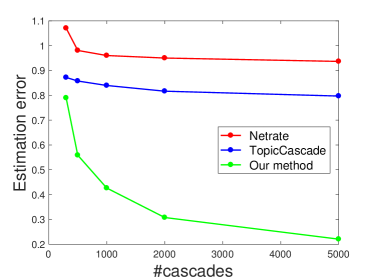
(b) Estimation error

Figure 4: Comparison of our method with Netrate and TopicCascade on Kronecker graph with parameter [0.8 0.6; 0.5 0.3].

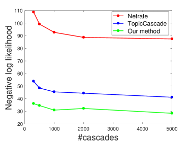
(a) Negative log-likelihood on test data set

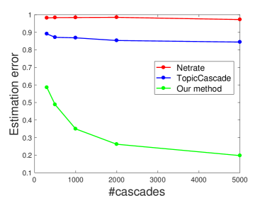
(b) Estimation error

Figure 5: Comparison of our method with Netrate and TopicCascade on Kronecker graph with parameter [0.7 0.7; 0.6 0.4].

Compare $g_{1}$ and $g_{2}$ regularizations.

Both $g_{1}$ and $g_{2}$ regularizers provide good estimates for $B_{1}$ and $B_{2}$. At optimum, the columns will have the same $\ell_{1}$ norm if $g_{1}$ is used, and the same $\ell_{2}$ norm if $g_{2}$ is used. In simulation, the performance of using $g_{1}$ or $g_{2}$ depends on whether the true parameter has the same $\ell_{1}$ or $\ell_{2}$ column norm. In practice, the columns of $B_{1}$ and $B_{2}$ could be balanced in a much more complicated way.

For the experiment, when using $g_{2}$, we set $s_{1}=1.5\cdot s_{1}^{*}$ and $s_{2}=1.5\cdot s_{2}^{*}$ where $s_{1}^{*}$ and $s_{2}^{*}$ are the true sparsity level of $B_{1}$ and $B_{2}$; when using $g_{1}$, for fair comparison, we set a fixed small regularization parameter $\lambda$. To illustrate the difference between $g_{1}$ and $g_{2}$, we set $p=50$ and evaluate the performance of Algorithm 1 with $g_{1}$ and Algorithm 2 with $g_{2}$ on different sample sizes. We scale the true $B_{1}^{*}$ and $B_{2}^{*}$ to have the same column sum ($\ell_{1}$ norm). Algorithm 2 is initialized with the solution of Algorithm 1. Figure 6 shows the comparison results on different sample sizes. We see that both methods performs well. When sample size is small, $g_{1}$ seems to be slightly better, since the true values are scaled to have the same $\ell_{1}$ column norm. When sample size is large, $g_{2}$ seems to be slightly better, since $\ell_{1}$ norm regularizer induces a biased solution.

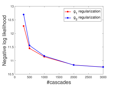
(a) Negative log-likelihood on test data set

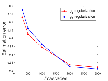
(b) Estimation error

Figure 6: Comparison of $g_{1}$ and $g_{2}$ regularizations.

Comparison with TopicCascade with enough samples.

Although our model is a special case of the topic-sensitive model, in the previous experiments, it seems like TopicCascade is not performing well even when sample size $n$ is large, especially on estimation error. We remark that the reason is that TopicCascade has $p^{2}K$ parameters, while our model has only $2pK$ parameters. With $p=200$, TopicCascade model has 100 times more parameters than ours. With such a large number of parameters, in order to obtain a sparse solution, we have to choose a large regularization in TopicCascade. Such a large regularization induces a large bias on the nonzero parameters, and therefore it worsens the performance of TopicCascade. Here we consider a lower dimensional model with $p=10,K=6$, and show that TopicCascade behaves similarly to our model when $n$ is large.

We repeat the experiment while keeping all the other settings unchanged. Figure 7 shows the comparison of the three methods with different sample sizes. We see that TopicCascade is almost as good as our method with large enough sample size. We also see that Netrate performs better when $p$ and $K$ are small, in terms of negative log-likelihood. This may be due to the small difference among topics, so one adjacency matrix suffices. However, the performance of Netrate is still bad in terms of estimation error. We also observe that the estimation error is not small even with small $p,K$ and large sample size. This may be due to only a few nodes being infected in each cascade, and therefore the effective information in each cascade is low.

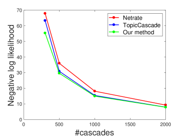
(a) Negative log-likelihood on test data set

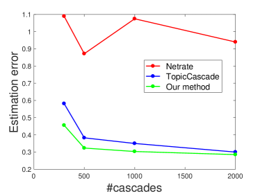
(b) Estimation error

Figure 7: Comparison of our method with Netrate and TopicCascade, with a small $p$.

Comparison of $F_{1}$ score.

We compare the three methods using $F_{1}$ score. The $F_{1}$ score is defined as the harmonic mean of $precision$ and $recall$: $F_{1}=2\cdot(precision^{-1}+recall^{-1})^{-1}$, where precision is the fraction of edges in the estimated network that is also in the true network; recall is the fraction of edges in the true network that is also in the estimated network. Since we have $K$ topics, we calculate the $F_{1}$ score of each $\{A_{k}\}_{k=1}^{K}$, and take the average. We would like to remark that the $F_{1}$ score is based on the estimated discrete network, while Netrate, TopicCascade, and our model estimate continuous parameters. Therefore, the $F_{1}$ score is not the main focus of the comparison. In Lasso, it is well known that one should choose a larger regularization parameter for variable selection consistency and a smaller regularization parameter for parameter estimation consistency (Meinshausen and Bühlmann, 2006). Similarly, to obtain a better $F_{1}$ score, we choose a larger regularization parameter.

For the experiments, we set $p=50$ and set the regularization parameter as 20 times the optimal one selected on the validation set for parameter estimation. Figure 8 shows the $F_{1}$ score of the three methods. We see that our method has the largest $F_{1}$ score even when the sample size is relatively small. With large enough sample size, both our method and TopicCascade can recover the network structure.

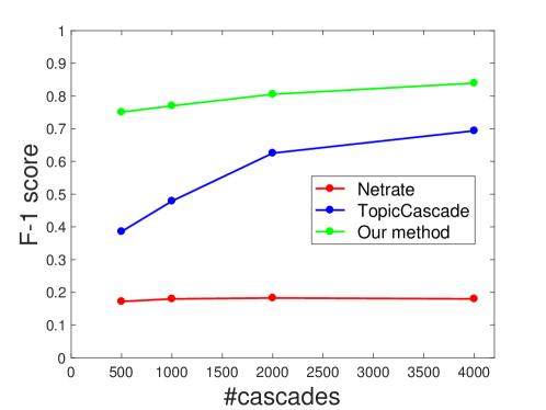
Figure 8: Comparison of our method with Netrate and TopicCascade on the $F_{1}$ score.

7.2 Running Time

We next compare the running times of the three methods. For fair comparison, for each method we set the step size, initialization, penalty $\lambda$, and tolerance level to be the same. Also one third of the samples are generated by each model. For our model we follow the data generation procedure as described before; for TopicCascade, for each topic $k$, we randomly select 5% of the components of $A^{k}$ to be nonzero, and these nonzero values are set as before as Unif$(0.8,1.8)\cdot\zeta$, where $\zeta=3$ with probability 0.3 and $\zeta=1$ with probability 0.7; for Netrate, we again randomly select 5% of the components of $A$ to be nonzero with values Unif$(0.8,1.8)\cdot\zeta$, and we randomly assign topic distributions. We run the three methods on 12 kernels. For Netrate and TopicCascade, since they are separable in each column, we run 12 columns in parallel; for our method, we calculate the gradient in parallel. We use our Algorithm 1 for our method and the proximal gradient algorithm for the other two methods, as suggested in Gomez-Rodriguez et al. (2016). We fix a baseline model size $n=500,p=50,K=10$, and set a free parameter $\xi$. For $\xi=\{1,2,5,8\}$, each time we increase $n,p$ by a factor of $\xi$ and record the running time (in seconds) of each method. Table 1 summarizes the results based on 5 replications in each setting. We can see that Netrate is the fastest because it does not consider the topic distribution. When $p$ becomes large, our algorithm is faster than TopicCascade and is of the same order as Netrate. This demonstrates that although our model is not separable in each column, it can still deal with large networks.

	$\xi=1$	$\xi=2$	$\xi=5$	$\xi=8$
Netrate	1.15	4.42	53.52	211.0
TopicCascade	5.43	36.10	153.03	1310.7
Our method	9.79	19.83	91.95	454.9

Table 1: Running time comparison (in sec).

8 Real World Data Set

In this section we evaluate our model on two real world data sets. We again focus on our proposed Algorithm 1.

8.1 Memetracker Data Set

The first data set is the MemeTracker data set (Leskovec et al., 2009). This data set contains 172 million news articles and blog posts from 1 million online sources over a period of one year from September 1, 2008 till August 31, 2009. Since the use of hyperlinks to refer to the source of information is relatively rare in mainstream media, the authors use the MemeTracker methodology (Leskovec and Sosic, 2016) to extract more than 343 million short textual phrases. After aggregating different textual variants of the same phrase, we consider each phrase cluster as a separate cascade $c$. Since all documents are time stamped, a cascade $c$ is simply a set of time-stamps when websites first mentioned a phrase in the phrase cluster $c$. Also since the diffusion rate of information on the internet usually reaches its peak when the information first comes out and decays rapidly, we use exponential transmission function here.

For our experiments we use the top 500 media sites and blogs with the largest 5000 cascades (phrase clusters). For each website we record the time when they first mention a phrase in the particular phrase cluster. We set the number of topic $K$ to be 10 as suggested in Du et al. (2013b), and perform Topic Modeling (LDA) to extract 10 most popular topics. We choose the regularization parameter $\lambda$ based on a hold-out validation set, and then use our Algorithm 1 to estimate the two node-topic matrices. The two matrices and the key words of the 10 topics are given in Tables 3 ($B_{1}$) and Table 4 ($B_{2}$). The keywords of the 10 topics are shown at the head of each table; the first column is the url of the website. Since LDA is a randomized algorithm, we run it several times and select the one that performs the best in separating the meaningful topics. We also manually adjust the top keywords a bit by removing a few trivial words, so that they are more informative. For example, the word “people” appears in several topics, and therefore we are not reporting it except for the seventh topic where “people” is the top-1 keyword. The websites above the center line in each table are the most popular websites. We have also hand-picked some less popular websites below the center line whose url suggest that they focus on specific topics, for example politics, business, sports, etc. The top websites are mostly web portals and they broadly post and cite news in many topics. Therefore to demonstrate that our model does extract some meaningful information, we select less popular websites below the center line and hope we can correctly extract the topics of interest of these specific websites.

From the two tables we can see that in general the influence matrix $B_{1}$ is much sparser than the receptivity matrix $B_{2}$, which means that websites tend to post news and blogs in many topics but only a few of them will be cited by others. The websites we hand pick are not as active as the top websites. Therefore the values for these websites are much smaller. For the top websites we only display entries which are above the threshold of 0.1, and leave smaller entries blank in the two tables; for the hand selected websites, only 0 values are left blank. From the two tables we see that our model performs quite well on those specific websites. For example the political websites have a large value on topic 4 (election); the business and economics websites have large value on topic 3 (economy), etc. Those “as expected” large values are shown in boldface in order to highlight them.

We then visualize the estimated $B_{1}$ and $B_{2}$ using t-SNE algorithm (van der Maaten and Hinton, 2008) to see whether nodes are clustered with respect to a set of topics, and whether the clusters in $B_{1}$ correspond to the ones in $B_{2}$. In $B_{1}$ and $B_{2}$, each row is a 10 dimensional vector corresponding to a website. We use t-SNE algorithm to give each website a location in a two-dimensional map and the scatter plot of $B_{1}$ and $B_{2}$ are given in Figure 9(a) and Figure 9(b). From the two figures we see that these points do not form clear clusters, which means most of the websites are in general interested in many of the topics and they do not differ too much from each other. We can see clearer clusters in the next example.

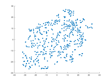
(a) Scatter plot of $B_{1}$

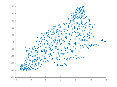
(b) Scatter plot of $B_{2}$

Figure 9: Scatter plot of $B_{1}$ and $B_{2}$ using t-SNE algorithm, for Memetracker data set.

	train	test	parameter	nonzero	AIC	BIC
Netrate	68.5	81.1	250000	20143	2.60$\times 10^{5}$	3.65$\times 10^{5}$
TopicCascade	62.5	81.8	2500000	142718	5.08$\times 10^{5}$	1.25$\times 10^{6}$
Our method	80.3	82.3	10000	7272	$\bm{2.38\times 10^{5}}$	$2.76\times 10^{5}$

Table 2: Comparison of the 3 methods on test cascades for Memetracker data set.

Finally we check the performance of our method on about 1500 test cascades and compare with Netrate and TopicCascade. Since the number of parameters are different for the three models, besides negative log-likelihood, we also use AIC and BIC as our metrics. Table 2 summarizes the results. The first column shows the names of the three methods and the following columns are the averaged negative log-likelihood on train set, averaged negative log-likelihood on test set, number of total parameters, number of nonzero parameters, AIC and BIC on test set calculated using the negative log-likelihood on test set (third column) and the number of nonzero parameters (fifth column).

From the table we see that our model has the largest negative log-likelihood on train set, and one reason for that is that our model have fewest parameters. However, we can see that both Netrate and TopicCascade are overfitting, while our method can generalize to test set with little overfitting. Our method uses much fewer parameters but has comparable negative log-likelihood on test, and also our method has the smallest AIC and BIC value.

	energy power oil gas	love man life time	market price money economy	obama mccain president party	think play team game	new technology system data	people clergy food problem	government law public state	life world church lord	time year student community
blog.myspace.com	0.29	0.17	0.17		0.11	0.25	0.54	0.12	0.24	0.43
us.rd.yahoo.com	0.7	0.33	0.24	0.18	0.15	0.38	0.28	0.4	0.42	0.61
news.google.com	0.15	0.13	0.15		0.13			0.15		0.65
startribune.com	0.42	0.59	0.5	0.3	0.32	0.49		0.24	0.31
news.com.au						0.12	0.18		0.2
breitbart.com	0.77	0.47		0.15	0.16	0.37		0.25	0.55
uk.news.yahoo.com	0.51	0.3	0.36		0.17	0.3	0.33	0.13		0.15
cnn.com	0.13	0.15	0.5	0.19			0.34			0.12
newsmeat.com				0.55
washingtonpost.com	0.10	0.41	0.14	0.10	0.10	0.39	0.13	0.23	0.22
forum.prisonplanet.com	0.2								0.17
news.originalsignal.com		0.13								0.17
c.moreover.com						0.19	0.24
philly.com
rss.feedsportal.com		0.1	0.14			0.15		0.18		0.19
foxnews.com	0.099	0.17	0.26	0.052	0.071					0.085
sports.espn.go.com		0.038		0.29	0.23		0.12	0.41
olympics.thestar.com				0.013	0.036					0.012
forbes.com	0.019		0.028		0.02				0.035
scienceblogs.com	0.24	0.14	0.077	0.2	0.12	0.15	0.092	0.052	0.29	0.091
swamppolitics.com				0.42	0.049
cqpolitics.com	0.016	0.23	0.082	0.16	0.23				0.045

Table 3: The influence matrix $B_{1}$ for Memetracker data set.

	energy power oil gas	love man life time	market price money economy	obama mccain president party	think play team game	new technology system data	people clergy food problem	government law public state	life world church lord	time year student community
blog.myspace.com	0.42	0.63	0.28	0.47	0.55	0.18	0.29	0.43	0.49	0.22
us.rd.yahoo.com	0.36	0.28	0.28	0.44	0.56	0.19	0.22	0.41	0.27	0.18
news.google.com	0.15		0.10	0.17				0.12	0.11
startribune.com	0.19	0.25	0.16	0.37	0.38	0.13	0.14	0.27	0.23	0.13
news.com.au		0.10		0.13	0.12
breitbart.com	0.14	0.13	0.14	0.3	0.2			0.16	0.18
uk.news.yahoo.com	0.12	0.14	0.15	0.21	0.14		0.14	0.14	0.13
cnn.com	0.12	0.15		0.18	0.16			0.15	0.12
newsmeat.com
washingtonpost.com	0.12	0.15	0.15	0.23	0.17	0.12	0.1	0.16	0.18
forum.prisonplanet.com				0.10					0.10
news.originalsignal.com	0.22	0.23	0.18	0.37	0.26		0.18	0.26	0.21
c.moreover.com	0.24	0.21	0.15	0.37	0.36	0.11	0.15	0.34	0.25	0.17
philly.com	0.11	0.15		0.16	0.21			0.14	0.11	0.1
rss.feedsportal.com		0.11		0.11		0.1			0.10
canadianbusiness.com	0.012		0.061			0.017	0.012	0.012
olympics.thestar.com		0.013			0.023			0.02	0.013
tech.originalsignal.com	0.036	0.032	0.04	0.031	0.038	0.13	0.037	0.037	0.043	0.031
businessweek.com	0.017		0.032	0.012	0.01	0.015	0.012	0.012	0.017
economy-finance.com	0.026	0.014	0.072	0.024	0.027	0.036		0.03	0.02
military.com		0.014		0.037	0.014			0.02	0.014	0.013
security.itworld.com						0.042				0.015
money.canoe.ca	0.011		0.022			0.02		0.012
computerworld.com	0.011					0.053

Table 4: The receptivity matrix $B_{2}$ for Memetracker data set.

8.2 Arxiv Citation Data Set

The second data set is the ArXiv high-energy physics theory citation network data set (Leskovec et al., 2005; Gehrke et al., 2003). This data set includes all papers published in ArXiv high-energy physics theory section from 1992 to 2003. We treat each author as a node and each publication as a cascade. For our experiments we use the top 500 authors with the largest 5000 cascades. For each author we record the time when they first cite a particular paper. Since it usually takes some time to publish papers we use Rayleigh transmission function here. We set the number of topic $K$ to be 6, and perform Topic Modeling on the abstracts of each paper to extract 6 most popular topics. We then use our Algorithm 1 to estimate the two node-topic matrices. The two matrices and the key words of the 6 topics are given in Tables 6 ($B_{1}$) and Table 7 ($B_{2}$). Again the keywords of the 6 topics are shown at the head of each table and the first column is the name of the author.

We compare the learned topics to the research interests listed by the authors in their website and we find that our model is able to discover the research topics of the authors accurately. For example Arkady Tseytlin reports string theory, quantum field theory and gauge theory; Shin’ichi Nojiri reports field theory; Burt A. Ovrut reports gauge theory; Amihay Hanany reports string theory; Ashoke Sen reports string theory and black holes as their research areas in their webpages. Moreover, Ashok Das has papers in supergravity, supersymmetry, string theory, and algebras; Ian Kogan has papers in string theory and boundary states; Gregory Moore has papers in algebras and non-commutativity. These are all successfully captured by our method.

We then again visualize the estimated $B_{1}$ and $B_{2}$ using t-SNE algorithm for which the scatter plots are shown in Figures 10. Here we see distinct patterns in the two figures. Figure 10(a) shows 6 “petals” corresponding to the authors interested in 6 topics, while the points in the center corresponds to the authors who have small influence on all the 6 topics. We therefore apply $K$-Means algorithm to get 7 clusters for the influence matrix $B_{1}$ as shown in Figure 10(a) (each color corresponds to one cluster), and then plot receptivity matrix $B_{2}$ in Figure 10(b) using these colors. We see that although Figure 10(b) also shows several clusters, the patterns are clearly different from Figure 10(a). This demonstrates the necessity of having different influence matrix $B_{1}$ and receptivity matrix $B_{2}$ in our model.

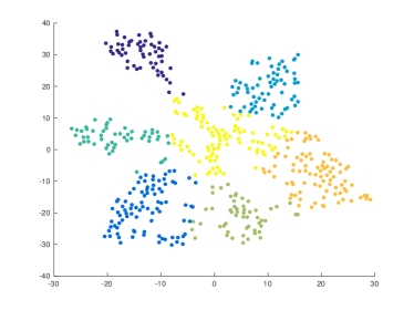
(a) Scatter plot of $B_{1}$

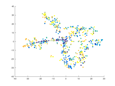
(b) Scatter plot of $B_{2}$

Figure 10: Scatter plot of $B_{1}$ and $B_{2}$ using t-SNE algorithm, for Citation data set.

Finally we check the performance of our method on about 1200 test cascades and compare with Netrate and TopicCascade. Table 5 summarizes the results. Similar as before, although Netrate and TopicCascade have smaller negative log-likelihood on train data, our method has the best performance on test data with significantly less parameters and little overfitting. So again we see that our model works quite well on this citation data set.

	train	test	parameter	nonzero	AIC	BIC
Netrate	66.8	83.9	250000	13793	2.34$\times 10^{5}$	3.05$\times 10^{5}$
TopicCascade	67.3	85.3	1500000	57052	3.24$\times 10^{5}$	6.16$\times 10^{5}$
Our method	78.2	82.3	6000	3738	$2.10\times 10^{5}$	$2.29\times 10^{5}$

Table 5: Comparison of the 3 methods on test cascades for citation data set.

	black hole energy chains	quantum model field theory	gauge theory field effective	algebra space group structure	states space noncommutative boundary	string theory supergravity supersymmetric
Christopher N. Pope	0.15	0.16	0.062	0.12
Hong Lu	0.11	0.16	0.067	0.12
Arkady Tseytlin	0.019	0.37	0.13	0.08		0.18
Sergei D. Odintsov		0.042	0.29		0.037	0.013
Shin’ichi Nojiri		0.028	0.22
Emilio Elizalde	0.012	0.023	0.11		0.14
Cumrun Vafa		0.17		0.43
Edward Witten	0.034	0.019		0.3	0.39	0.036
Ashok Das	0.065	0.018		0.038		0.14
Sergio Ferrara	0.41	0.056		0.2	0.11
Renata Kallosh	0.16	0.49	0.17	0.11	0.029
Mirjam Cvetic		0.35	0.04	0.032		0.026
Burt A. Ovrut		0.11	0.23	0.083
Ergin Sezgin	0.16	0.25	0.54
Ian Kogan	0.013				0.14	0.11
Gregory Moore				0.04	0.18
I. Antoniadis	0.21	0.084	0.13	0.32	0.07	0.22
Andrew Strominger		0.37		0.2
Barton Zwiebach	0.027		0.015	0.15	0.2
Paul Townsend	0.036	0.72	0.65	0.21
Robert Myers		0.075	0.023	0.018
Eric Bergshoeff	0.096	0.062	0.12	0.092
Amihay Hanany				0.16	0.049	0.22
Ashoke Sen	0.11	0.15		0.48		0.22

Table 6: The influence matrix $B_{1}$ for citation data set.

	black hole energy chains	quantum model field theory	gauge theory field effective	algebra space group structure	states space noncommutative boundary	string theory supergravity supersymmetric
Christopher N. Pope	0.5	0.78	0.062	0.26
Hong Lu	0.47	0.86	0.045	0.25
Arkady Tseytlin	0.23	0.88	0.55	0.3	0.26
Sergei D. Odintsov		0.58	0.80	0.029	0.14	0.16
Shin’ichi Nojiri		0.29	0.35	0.021		0.17
Emilio Elizalde		0.037	0.18		0.24	0.019
Cumrun Vafa	0.098			0.64	0.087	0.16
Edward Witten	0.097		0.29	0.41	0.28	0.2
Ashok Das	0.2	0.099	0.11	0.023		0.14
Sergio Ferrara	0.51	0.3	0.041	0.53	0.13
Renata Kallosh	0.19	0.3	0.58	0.16
Mirjam Cvetic	0.029	1.4	0.077	0.31		0.095
Burt A. Ovrut	0.021	0.17	0.34	0.13		0.12
Ergin Sezgin	0.17	0.062	0.38	0.1
Ian Kogan	0.061	0.3		0.05	0.42	0.13
Gregory Moore	0.27	0.064	0.28	0.51	0.38	0.056
I. Antoniadis	0.1	0.024	0.042	0.23		0.1
Andrew Strominger	0.032	0.58	0.078	0.1	0.079
Barton Zwiebach	0.14		0.018	0.096	0.021	0.068
Paul Townsend	0.06	0.12	0.42	0.21
Robert Myers		0.86	0.2	0.23	0.042	0.04
Eric Bergshoeff	0.24	0.15	0.82	0.27	0.011
Amihay Hanany				0.65	0.02	0.22
Ashoke Sen		0.057		0.16	0.051	0.04

Table 7: The receptivity matrix $B_{2}$ for citation data set.

9 Conclusion

The majority of work on information diffusion has focused on recovering the diffusion matrix while ignoring the structure among nodes. In this paper, we propose an influence-receptivity model that takes the structure among nodes into consideration. We develop two efficient algorithms and prove that the iterates of the algorithm converge linearly to the true value up to a statistical error. Experimentally, we demonstrate that our model performs well in both synthetic and real data, and produces a more interpretable model.

There are several interesting research threads we plan to pursue. In terms of modeling, an interesting future direction would be to allow each cascade to have a different propagation rate. In our current model, two cascades with the same topic distribution will have the same diffusion behavior. In real world, we expect some information to be intrinsically more interesting and hence spread much faster. Another extension would be allowing dynamic influence-receptivity matrices over time. Finally, all existing work on network structure recovery from cascades assumes that the first node observed to be infected is the source of the diffusion. In many scenarios, the source may be latent and directly infect many nodes. Extending our model to incorporate this feature is work in progress.

Acknowledgments

We are extremely grateful to the associate editor, Boaz Nadler, and two anonymous reviewers for their insightful comments that helped improve this paper. This work is partially supported by an IBM Corporation Faculty Research Fund and the William S. Fishman Faculty Research Fund at the University of Chicago Booth School of Business. This work was completed in part with resources provided by the University of Chicago Research Computing Center.

A Technical proofs

A.1 Proof of Theorem 3.

Since $f(\Theta)$ is strongly convex in $\Theta$, we have

$$f(\widehat{\Theta})-f(\Theta^{*})-\big{\langle}\nabla f(\Theta^{*}),\widehat{\Theta}-\Theta^{*}\big{\rangle}\geq\frac{\mu}{2}\big{\|}\widehat{\Theta}-\Theta^{*}\big{\|}_{F}^{2}.$$ (39)

On the other hand, since $\widehat{\Theta}$ is the global minimum, we have

$$f(\widehat{\Theta})\leq f(\Theta^{*}).$$ (40)

Combining the above two inequalities, we obtain

$$\frac{\mu}{2}\big{\|}\widehat{\Theta}-\Theta^{*}\big{\|}_{F}^{2}\leq-\big{\langle}\nabla f(\Theta^{*}),\widehat{\Theta}-\Theta^{*}\big{\rangle}\leq\big{\|}\nabla f(\Theta^{*})\big{\|}_{F}\cdot\big{\|}\widehat{\Theta}-\Theta^{*}\big{\|}_{F}$$ (41)

and

$$\big{\|}\widehat{\Theta}-\Theta^{*}\big{\|}_{F}\leq\frac{2}{\mu}\big{\|}\nabla f(\Theta^{*})\big{\|}_{F}.$$ (42)

This shows that for any $k$, we have

$$\big{\|}\widehat{\Theta}_{k}-\Theta_{k}^{*}\big{\|}_{F}\leq\frac{2}{\mu}\big{\|}\nabla f(\Theta^{*})\big{\|}_{F}.$$ (43)

According to the construction of the initialization point, the rank-1 SVD of $\Theta_{k}$ is given by $\sigma_{k}u_{k}v_{k}^{\top}$. Since it is the best rank-1 approximation of $\widehat{\Theta}_{k}$, we have that

$$\big{\|}\sigma_{k}u_{k}v_{k}^{\top}-\widehat{\Theta}_{k}\big{\|}_{F}\leq\big{\|}\widehat{\Theta}_{k}-\Theta_{k}^{*}\big{\|}_{F}.$$ (44)

By the triangular inequality

$$\big{\|}\sigma_{k}u_{k}v_{k}^{\top}-\Theta_{k}^{*}\big{\|}_{F}\leq\big{\|}\sigma_{k}u_{k}v_{k}^{\top}-\widehat{\Theta}_{k}\big{\|}_{F}+\big{\|}\widehat{\Theta}_{k}-\Theta_{k}^{*}\big{\|}_{F}\leq 2\big{\|}\widehat{\Theta}_{k}-\Theta_{k}^{*}\big{\|}_{F}\leq\frac{4}{\mu}\big{\|}\nabla f(\Theta^{*})\big{\|}_{F}.$$ (45)

Then by Lemma 5.14 in Tu et al. (2016) we have

$$\big{\|}{b_{k}^{1}}^{(0)}-{b_{k}^{1}}^{*}\big{\|}_{2}^{2}+\big{\|}{b_{k}^{2}}^{(0)}-{b_{k}^{2}}^{*}\big{\|}_{2}^{2}\leq\frac{2}{\sqrt{2}-1}\cdot\frac{\big{\|}\sigma_{k}u_{k}v_{k}^{\top}-\Theta_{k}^{*}\big{\|}_{F}^{2}}{\|\Theta_{k}^{*}\|_{2}}.$$ (46)

Let $\sigma^{*}=\min_{k}\|\Theta_{k}^{*}\|_{2}$. Using Lemma 3.3 in Li et al. (2016), we have the following upper bound on the initialization $B^{(0)}=\big{[}B_{1}^{(0)},B_{2}^{(0)}\big{]}$,

$$d^{2}\big{(}B^{(0)},B^{*}\big{)}\leq\xi^{2}\cdot\frac{2K}{\sqrt{2}-1}\cdot\frac{16\big{\|}\nabla f(\Theta^{*})\big{\|}_{F}^{2}}{\mu^{2}\sigma^{*}}\leq\frac{80\xi^{2}K\big{\|}\nabla f(\Theta^{*})\big{\|}_{F}^{2}}{\mu^{2}\sigma^{*}},$$ (47)

where $\xi$ is defined as $\xi^{2}=1+\frac{2}{\sqrt{c-1}}$ with $c$ set as $s=cs^{*}$ as in Theorem 4.

A.2 Proof of Theorem 4.

The key part of the proof is to quantify the estimation error after one iteration. We then iteratively apply this error bound. For notation simplicity, we omit the superscript indicating the iteration number $t$ when quantifying the iteration error. We denote the current iterate as $B=[B_{1},B_{2}]$ and the next iterate as $B^{+}=[B_{1}^{+},B_{2}^{+}]$. Recall that the true values are given by $B^{*}=[B_{1}^{*},B_{2}^{*}]$ with columns given by ${b_{k}^{1}}^{*},{b_{k}^{2}}^{*}$. The $k^{\text{th}}$ columns of $B_{1},B_{2},B_{1}^{+},B_{2}^{+}$ are denoted as $b_{k}^{1},b_{k}^{2},b_{k}^{1+},b_{k}^{2+}$. We use $b_{k}$ and $b_{k}^{+}$ to denote $b_{k}=[b_{k}^{1},b_{k}^{2}]$ and $b_{k}^{+}=[b_{k}^{1+},b_{k}^{2+}]$.

According to the update rule given in Algorithm 2, we have

$$B_{1}^{+} =\text{Hard}\Big{(}B_{1}-\eta\cdot\nabla_{B_{1}}f\big{(}B_{1},B_{2}\big{)}-\eta\cdot\nabla_{B_{1}}g\big{(}B_{1},B_{2}\big{)},s\Big{)},$$ (48)

$$B_{2}^{+} =\text{Hard}\Big{(}B_{2}-\eta\cdot\nabla_{B_{2}}f\big{(}B_{1},B_{2}\big{)}-\eta\cdot\nabla_{B_{2}}g\big{(}B_{1},B_{2}\big{)},s\Big{)},$$ (49)

with the regularization term $g(B_{1},B_{2})=\frac{1}{4}\cdot\sum_{k=1}^{K}\Big{(}\big{\|}b^{1}_{k}\big{\|}_{2}^{2}-\big{\|}b^{2}_{k}\big{\|}_{2}^{2}\Big{)}^{2}$ given in (17). Note that, since the true values $B_{1}^{*},B_{2}^{*}$ are nonnegative and the negative values only make the estimation accuracy worse, we can safely ignore the operation $[B]_{+}$ in the theoretical analysis. Moreover, when quantifying the estimation error after one iteration, we assume that the current estimate $B$ is not too far away from the true value $B^{*}$ in that

$$d^{2}(B,B^{*})\leq{\frac{1}{4}\gamma\sigma^{*}}\cdot\min\Big{\{}1,\frac{1}{4(\mu+L)}\Big{\}},$$ (50)

where $\gamma=\min\{1,\mu L/(\mu+L)\}$ and $\sigma^{*}=\min_{k}\|\Theta_{k}^{*}\|_{2}$. This upper bound (50) is satisfied for $B^{(0)}$ when the sample size is large enough, as assumed in (30). In the proof, we will show that (50) is also satisfied in each iteration of Algorithm 2. Therefore we can recursively apply the estimation error bound for one iteration.

Let

$$S_{1}=\text{supp}(B_{1})\cup\text{supp}(B_{1}^{+})\cup\text{supp}(B_{1}^{*})~{}\text{ and }~{}S_{2}=\text{supp}(B_{2})\cup\text{supp}(B_{2}^{+})\cup\text{supp}(B_{2}^{*})$$

denote the nonzero positions of the current iterate, next iterate, and the true value. Similarly, let

$$S_{1k}=\text{supp}(b^{1}_{k})\cup\text{supp}(b_{k}^{1+})\cup\text{supp}(b_{k}^{1*})\text{ and }S_{2k}=\text{supp}(b^{2}_{k})\cup\text{supp}(b_{k}^{2+})\cup\text{supp}(b_{k}^{2*})$$

capture the support for the $k^{\text{th}}$ column. With this notation, we have

$$d^{2}(B^{+},B^{*}) =\big{\|}B_{1}^{+}-B_{1}^{*}\big{\|}_{F}^{2}+\big{\|}B_{2}^{+}-B_{2}^{*}\big{\|}_{F}^{2}$$ (51)

$$\leq\xi^{2}\Big{(}\big{\|}B_{1}-B_{1}^{*}-\eta\cdot\big{[}\nabla_{B_{1}}f\big{(}B_{1},B_{2}\big{)}+\nabla_{B_{1}}g\big{(}B_{1},B_{2}\big{)}\big{]}_{S_{1}}\big{\|}_{F}^{2}$$

$$\qquad\qquad\qquad+\big{\|}B_{2}-B_{2}^{*}-\eta\cdot\big{[}\nabla_{B_{2}}f\big{(}B_{1},B_{2}\big{)}+\nabla_{B_{2}}g\big{(}B_{1},B_{2}\big{)}\big{]}_{S_{2}}\big{\|}_{F}^{2}\Big{)}$$

$$\leq\xi^{2}\Big{(}d^{2}(B,B^{*})-2\eta\cdot\big{\langle}\nabla_{B}f\big{(}B\big{)}+\nabla_{B}g\big{(}B\big{)},B-B^{*}\big{\rangle}_{S_{1}\cup S_{2}}$$

$$\qquad\qquad\qquad+\eta^{2}\cdot\big{\|}\big{[}\nabla_{B}f\big{(}B\big{)}+\nabla_{B}g\big{(}B\big{)}\big{]}_{S_{1}\cup S_{2}}\big{\|}_{F}^{2}\Big{)}$$

$$\leq\xi^{2}\Big{(}d^{2}(B,B^{*})-2\eta\cdot\big{\langle}\nabla_{B}f\big{(}B\big{)}+\nabla_{B}g\big{(}B\big{)},B-B^{*}\big{\rangle}_{S_{1}\cup S_{2}}$$

$$\qquad\qquad\qquad+2\eta^{2}\cdot\big{\|}\big{[}\nabla_{B}f\big{(}B\big{)}\big{]}_{S_{1}\cup S_{2}}\big{\|}_{F}^{2}+2\eta^{2}\cdot\big{\|}\big{[}\nabla_{B}g\big{(}B\big{)}\big{]}_{S_{1}\cup S_{2}}\big{\|}_{F}^{2}\Big{)},$$

where the first inequality follows from Lemma 3.3 of Li et al. (2016) and $\xi$ is defined as $\xi^{2}=1+\frac{2}{\sqrt{c-1}}$ with $c$ set as $s=cs^{*}$.

Different from the existing work on matrix factorization that focuses on recovery of a single rank-$K$ matrix, in our model, we have $K$ rank-1 matrices. Therefore we have to deal with each column of $B_{1}$ and $B_{2}$ separately. With some abuse of notation, we denote $f_{k}(b_{k})=f_{k}(b_{k}^{1},b_{k}^{2})=f_{k}(\Theta_{k})=f(\Theta_{1},\ldots,\Theta_{k},\ldots,\Theta_{K})$ as a function of the $k^{\text{th}}$ columns of $B_{1},B_{2}$, with all the other columns fixed. The gradient of $f_{k}(\Theta_{k})$ with respect to $b_{k}^{1}$ is then given by $\nabla f_{k}(\Theta_{k})\cdot b_{k}^{2}$. Similarly, we denote

$$g_{k}(b_{k})=g_{k}(b_{k}^{1},b_{k}^{2})=\frac{1}{4}\Big{(}\big{\|}b^{1}_{k}\big{\|}_{2}^{2}-\big{\|}b^{2}_{k}\big{\|}_{2}^{2}\Big{)}^{2},$$ (52)

such that $g(B_{1},B_{2})=\sum_{k=1}^{K}g_{k}(b_{k})$.

We first deal the terms involving regularization $g(\cdot)$ in (51). Denote $\Delta b_{k}=\big{\|}b^{1}_{k}\big{\|}_{2}^{2}-\big{\|}b^{2}_{k}\big{\|}_{2}^{2}$, so that $g_{k}(b_{k})=\frac{1}{4}(\Delta b_{k})^{2}$. Then

$$\Big{\|}\big{[}\nabla_{B}g\big{(}B\big{)}\big{]}_{S_{1}\cup S_{2}}\Big{\|}_{F}^{2}\leq\sum_{k=1}^{K}\|\nabla g_{k}(b_{k})\|_{F}^{2}\leq\sum_{k=1}^{K}(\Delta b_{k})^{2}\cdot\|b_{k}\|_{2}^{2}\leq\|B\|_{2}^{2}\cdot\sum_{k=1}^{K}(\Delta b_{k})^{2}.$$ (53)

Equation (36) in the proof of Lemma B.1 in Park et al. (2018) gives us

$$\big{\langle}\nabla_{B}g\big{(}B\big{)},B-B^{*}\big{\rangle}_{S_{1}\cup S_{2}}\geq\sum_{k=1}^{K}\Big{[}\frac{5}{8}(\Delta b_{k})^{2}-\frac{1}{2}\Delta b_{k}\cdot\|b_{k}-b_{k}^{*}\|_{2}^{2}\Big{]}.$$ (54)

We then bound the two terms in (54). For the first term, we have

$$(\Delta b_{k})^{2} \geq\big{\|}b_{k}^{1}{b_{k}^{1}}^{\top}-{b_{k}^{1}}^{*}{{b_{k}^{1}}^{*}}^{\top}\big{\|}_{F}^{2}+\big{\|}b_{k}^{2}{b_{k}^{2}}^{\top}-{b_{k}^{2}}^{*}{{b_{k}^{2}}^{*}}^{\top}\big{\|}_{F}^{2}-2\big{\|}b_{k}^{1}{b_{k}^{2}}^{\top}-{b_{k}^{1}}^{*}{{b_{k}^{2}}^{*}}^{\top}\big{\|}_{F}^{2}$$ (55)

$$\geq\gamma\cdot\Big{(}\big{\|}b_{k}^{1}{b_{k}^{1}}^{\top}-{b_{k}^{1}}^{*}{{b_{k}^{1}}^{*}}^{\top}\big{\|}_{F}^{2}+\big{\|}b_{k}^{2}{b_{k}^{2}}^{\top}-{b_{k}^{2}}^{*}{{b_{k}^{2}}^{*}}^{\top}\big{\|}_{F}^{2}+2\big{\|}b_{k}^{1}{b_{k}^{2}}^{\top}-{b_{k}^{1}}^{*}{{b_{k}^{2}}^{*}}^{\top}\big{\|}_{F}^{2}\Big{)}$$

$$\qquad\qquad-\frac{4\mu L}{\mu+L}\big{\|}b_{k}^{1}{b_{k}^{2}}^{\top}-{b_{k}^{1}}^{*}{{b_{k}^{2}}^{*}}^{\top}\big{\|}_{F}^{2}$$

$$\geq\frac{3}{2}\gamma\big{\|}\Theta_{k}^{*}\big{\|}_{2}\cdot\Big{(}\big{\|}b_{k}^{1}-{b_{k}^{1}}^{*}\big{\|}_{2}^{2}+\big{\|}b_{k}^{2}-{b_{k}^{2}}^{*}\big{\|}_{2}^{2}\Big{)}-\frac{4\mu L}{\mu+L}\big{\|}b_{k}^{1}{b_{k}^{2}}^{\top}-{b_{k}^{1}}^{*}{{b_{k}^{2}}^{*}}^{\top}\big{\|}_{F}^{2},$$

where the last inequality follows from Lemma 5.1 in Tu et al. (2016), and $\gamma=\min\{1,\mu L/(\mu+L)\}$ as before. For the second term in (54), recall that the current iterate satisfies the condition (50), so that

$$\frac{1}{2}\Delta b_{k}\cdot\|b_{k}-b_{k}^{*}\|_{2}^{2} \leq\frac{1}{2}\Delta b_{k}\cdot\|b_{k}-b_{k}^{*}\|_{2}\cdot\sqrt{\frac{1}{4}\gamma\sigma^{*}}$$ (56)

$$\leq\frac{1}{16}\gamma\sigma^{*}\cdot\|b_{k}-b_{k}^{*}\|_{2}^{2}+\frac{1}{4}(\Delta b_{k})^{2}.$$

Plugging (56) and (55) into (54) and summing over $k$, we obtain

$$\big{\langle}\nabla_{B}g\big{(}B\big{)},B-B^{*}\big{\rangle}_{S_{1}\cup S_{2}} \geq\frac{3}{8}\sum_{k=1}^{K}(\Delta b_{k})^{2}-\frac{1}{16}\sum_{k=1}^{K}\gamma\sigma^{*}\cdot\|b_{k}-b_{k}^{*}\|_{2}^{2}$$ (57)

$$=\frac{1}{4}\sum_{k=1}^{K}(\Delta b_{k})^{2}+\frac{1}{8}\sum_{k=1}^{K}(\Delta b_{k})^{2}-\frac{1}{16}\gamma\sigma^{*}\cdot d^{2}(B,B^{*})$$

$$\geq\frac{1}{8}\gamma\sigma^{*}d^{2}(B,B^{*})-\frac{\mu L}{2(\mu+L)}\big{\|}b_{k}^{1}{b_{k}^{2}}^{\top}-{b_{k}^{1}}^{*}{{b_{k}^{2}}^{*}}^{\top}\big{\|}_{F}^{2}+\frac{1}{4}\sum_{k=1}^{K}(\Delta b_{k})^{2}.$$

Together with (53), we obtain

$$-2\eta\big{\langle}\nabla_{B}g\big{(}B\big{)},B-B^{*}\big{\rangle}_{S_{1}\cup S_{2}}+2\eta^{2}\Big{\|}\big{[}\nabla_{B}g\big{(}B\big{)}\big{]}_{S_{1}\cup S_{2}}\Big{\|}_{F}^{2}$$ (58)

$$\qquad\leq-\frac{1}{4}\eta\gamma\sigma^{*}d^{2}(B,B^{*})+\eta\frac{\mu L}{\mu+L}\big{\|}b_{k}^{1}{b_{k}^{2}}^{\top}-{b_{k}^{1}}^{*}{{b_{k}^{2}}^{*}}^{\top}\big{\|}_{F}^{2}+\Big{(}2\eta^{2}\|B\|_{2}^{2}-\frac{1}{2}\eta\Big{)}\sum_{k=1}^{K}(\Delta b_{k})^{2}.$$

Next, we upper bound the terms in (51) involving the objective function $f(\cdot)$. For the inner product term, for each $k$, we have

$$\Big{\langle}[\nabla f_{k}(b_{k}^{1}{b_{k}^{2}}^{\top})\cdot b_{k}^{2}]_{S_{1}},b_{k}^{1}-{b_{k}^{1}}^{*}\Big{\rangle}+\Big{\langle}[\nabla f_{k}(b_{k}^{1}{b_{k}^{2}}^{\top})\cdot b_{k}^{1}]_{S_{2}},b_{k}^{2}-{b_{k}^{2}}^{*}\Big{\rangle}$$ (59)

$$=\Big{\langle}\nabla f_{k}(b_{k}^{1}{b_{k}^{2}}^{\top}),(b_{k}^{1}-{b_{k}^{1}}^{*}){b_{k}^{2}}^{\top}+b_{k}^{1}({b_{k}^{2}-{b_{k}^{2}}^{*}})^{\top}\Big{\rangle}_{S_{1k},S_{2k}}$$

$$=\Big{\langle}\nabla f_{k}(b_{k}^{1}{b_{k}^{2}}^{\top}),(b_{k}^{1}-{b_{k}^{1}}^{*})({b_{k}^{2}-{b_{k}^{2}}^{*}})^{\top}+b_{k}^{1}{b_{k}^{2}}^{\top}-{b_{k}^{1}}^{*}{{b_{k}^{2}}^{*}}^{\top}\Big{\rangle}_{S_{1k},S_{2k}}$$

$$=\Big{\langle}\nabla f_{k}(b_{k}^{1}{b_{k}^{2}}^{\top}),(b_{k}^{1}-{b_{k}^{1}}^{*})({b_{k}^{2}-{b_{k}^{2}}^{*}})^{\top}\Big{\rangle}_{S_{1k},S_{2k}}+\Big{\langle}\nabla f_{k}(b_{k}^{1}{b_{k}^{2}}^{\top}),b_{k}^{1}{b_{k}^{2}}^{\top}-{b_{k}^{1}}^{*}{{b_{k}^{2}}^{*}}^{\top}\Big{\rangle}_{S_{1k},S_{2k}}$$

$$=\underbrace{\Big{\langle}\nabla f_{k}(b_{k}^{1}{b_{k}^{2}}^{\top}),(b_{k}^{1}-{b_{k}^{1}}^{*})({b_{k}^{2}-{b_{k}^{2}}^{*}})^{\top}\Big{\rangle}_{S_{1k},S_{2k}}}_{W_{1k}}+\underbrace{\Big{\langle}\nabla f_{k}({b_{k}^{1}}^{*}{{b_{k}^{2}}^{*}}^{\top}),b_{k}^{1}{b_{k}^{2}}^{\top}-{b_{k}^{1}}^{*}{{b_{k}^{2}}^{*}}^{\top}\Big{\rangle}_{S_{1k},S_{2k}}}_{W_{2k}}$$

$$\qquad\qquad\qquad+\underbrace{\Big{\langle}\nabla f_{k}(b_{k}^{1}{b_{k}^{2}}^{\top})-\nabla f_{k}({b_{k}^{1}}^{*}{{b_{k}^{2}}^{*}}^{\top}),b_{k}^{1}{b_{k}^{2}}^{\top}-{b_{k}^{1}}^{*}{{b_{k}^{2}}^{*}}^{\top}\Big{\rangle}_{S_{1k},S_{2k}}}_{W_{3k}}.$$

For the term $W_{3k}$, Theorem 2.1.11 of Nesterov (2004) gives

$$W_{3k} \geq\frac{\mu L}{\mu+L}\cdot\Big{\|}{b_{k}^{1}{b_{k}^{2}}^{\top}-{b_{k}^{1}}^{*}{{b_{k}^{2}}^{*}}^{\top}}\Big{\|}_{F}^{2}+\frac{1}{\mu+L}\cdot\Big{\|}\left[\nabla f(b_{k}^{1}{b_{k}^{2}}^{\top})-\nabla f({b_{k}^{1}}^{*}{{b_{k}^{2}}^{*}}^{\top})\right]_{S_{1k},S_{2k}}\Big{\|}_{F}^{2}.$$ (60)

For the term $W_{2k}$, according to the definition of the statistical error in (26), we have

$$\sum_{k=1}^{K}W_{2k} \geq-e_{\rm stat}\cdot\sum_{k=1}^{K}\Big{\|}b_{k}^{1}{b_{k}^{2}}^{\top}-{b_{k}^{1}}^{*}{{b_{k}^{2}}^{*}}^{\top}\Big{\|}_{F}$$ (61)

$$\geq-\frac{K}{2}\frac{\mu+L}{\mu L}e_{\rm stat}^{2}-\frac{1}{2}\frac{\mu L}{\mu+L}\sum_{k=1}^{K}\Big{\|}{b_{k}^{1}{b_{k}^{2}}^{\top}-{b_{k}^{1}}^{*}{{b_{k}^{2}}^{*}}^{\top}}\Big{\|}_{F}^{2}.$$

For the term $W_{1k}$,

$$\sum_{k=1}^{K}W_{1k} =\sum_{k=1}^{K}\Big{\langle}\nabla f_{k}({b_{k}^{1}}^{*}{{b_{k}^{2}}^{*}}^{\top}),(b_{k}^{1}-{b_{k}^{1}}^{*})({b_{k}^{2}-{b_{k}^{2}}^{*}})^{\top}\Big{\rangle}_{S_{1k},S_{2k}}$$ (62)

$$\qquad\qquad\qquad+\Big{\langle}\nabla f_{k}(b_{k}^{1}{b_{k}^{2}}^{\top})-\nabla f_{k}({b_{k}^{1}}^{*}{{b_{k}^{2}}^{*}}^{\top}),(b_{k}^{1}-{b_{k}^{1}}^{*})({b_{k}^{2}-{b_{k}^{2}}^{*}})^{\top}\Big{\rangle}_{S_{1k},S_{2k}}$$

$$\geq-\left(e_{\rm stat}+\sum_{k=1}^{K}\Big{\|}\left[\nabla f_{k}(b_{k}^{1}{b_{k}^{2}}^{\top})-\nabla f_{k}({b_{k}^{1}}^{*}{{b_{k}^{2}}^{*}}^{\top})\right]_{S_{1k},S_{2k}}\Big{\|}_{F}\right)\cdot d^{2}(B,B^{*})$$

$$\geq-\left(e_{\rm stat}+\sum_{k=1}^{K}\Big{\|}\left[\nabla f_{k}(b_{k}^{1}{b_{k}^{2}}^{\top})-\nabla f_{k}({b_{k}^{1}}^{*}{{b_{k}^{2}}^{*}}^{\top})\right]_{S_{1k},S_{2k}}\Big{\|}_{F}\right)\sqrt{\frac{\gamma\sigma^{*}}{16(\mu+L)}}d(B,B^{*})$$

$$\geq-\frac{K}{2(\mu+L)}\cdot\left(e_{\rm stat}^{2}+\sum_{k=1}^{K}\Big{\|}\left[\nabla f_{k}(b_{k}^{1}{b_{k}^{2}}^{\top})-\nabla f_{k}({b_{k}^{1}}^{*}{{b_{k}^{2}}^{*}}^{\top})\right]_{S_{1k},S_{2k}}\Big{\|}_{F}^{2}\right)$$

$$\qquad\qquad\qquad\qquad\qquad\qquad\qquad\qquad\qquad\qquad\qquad\qquad-\frac{1}{16}\gamma\sigma^{*}\cdot d^{2}(B,B^{*}),$$

where we use the fact that $d(B,B^{*})$ satisfies (50),

$$\big{\|}(b_{k}^{1}-{b_{k}^{1}}^{*})({b_{k}^{2}-{b_{k}^{2}}^{*}})^{\top}\big{\|}_{F}\leq\big{\|}b_{k}^{1}-{b_{k}^{1}}^{*}\big{\|}_{F}\big{\|}{b_{k}^{2}-{b_{k}^{2}}^{*}}\big{\|}_{F}\leq\big{\|}b_{k}^{1}-{b_{k}^{1}}^{*}\big{\|}_{F}^{2}+\big{\|}{b_{k}^{2}-{b_{k}^{2}}^{*}}\big{\|}_{F}^{2},$$ (63)

and that their summation is $d^{2}(B,B^{*})$. For the term in (51) involving square of $f(\cdot)$, we have

$$\Big{\|}\big{[}\nabla_{B}f\big{(}B\big{)}\big{]}_{S_{1}\cup S_{2}}\Big{\|}_{F}^{2}\leq 4\cdot\Big{(}\sum_{k=1}^{K}\Big{\|}\left[\nabla f(b_{k}^{1}{b_{k}^{2}}^{\top})-\nabla f({b_{k}^{1}}^{*}{{b_{k}^{2}}^{*}}^{\top})\right]_{S_{1},S_{2}}\Big{\|}_{F}^{2}+e_{\text{stat}}^{2}\Big{)}\cdot\|B\|_{2}^{2}.$$ (64)

Combining (60), (61), (62), and (64), we obtain

$$-2\eta\big{\langle}\nabla_{B}f\big{(}B\big{)},B-B^{*}\big{\rangle}_{S_{1}\cup S_{2}}+\eta^{2}\Big{\|}\big{[}\nabla_{B}f\big{(}B\big{)}\big{]}_{S_{1}\cup S_{2}}\Big{\|}_{F}^{2}$$ (65)

$$\leq e_{\text{stat}}^{2}\cdot\Big{(}8\|B\|_{2}^{2}\eta^{2}+\frac{K(\mu+L)}{\mu L}\eta+\frac{K}{\mu+L}\eta\Big{)}$$

$$\qquad\qquad-\frac{\mu L}{\mu+L}\eta\sum_{k=1}^{K}\Big{\|}{b_{k}^{1}{b_{k}^{2}}^{\top}-{b_{k}^{1}}^{*}{{b_{k}^{2}}^{*}}^{\top}}\Big{\|}_{F}^{2}+\frac{1}{8}\gamma\sigma^{*}\eta\cdot d^{2}(B,B^{*})$$

$$\qquad\qquad+\Big{(}8\eta^{2}\|B\|_{2}^{2}-\frac{K\eta}{\mu+L}\Big{)}\sum_{k=1}^{K}\Big{\|}\left[\nabla f_{k}(b_{k}^{1}{b_{k}^{2}}^{\top})-\nabla f_{k}({b_{k}^{1}}^{*}{{b_{k}^{2}}^{*}}^{\top})\right]_{S_{1k},S_{2k}}\Big{\|}_{F}^{2}.$$

Plugging (LABEL:eq:one_iterate_G) and (LABEL:eq:one_iterate_F) into (51), we obtain

$$d^{2}(B^{+},B^{*}) =\xi^{2}\left(1-\frac{1}{4}\gamma\sigma^{*}\eta\right)\cdot d^{2}(B,B^{*})+\xi^{2}\Big{(}2\eta^{2}\|B\|_{2}^{2}-\frac{1}{2}\eta\Big{)}\sum_{k=1}^{K}(\Delta b_{k})^{2}$$ (66)

$$\qquad+\xi^{2}\left(8\eta^{2}\cdot\|B\|_{2}^{2}-\frac{K\eta}{\mu+L}\right)\cdot\sum_{k=1}^{K}\Big{\|}\left[\nabla f_{k}(b_{k}^{1}{b_{k}^{2}}^{\top})-\nabla f_{k}({b_{k}^{1}}^{*}{{b_{k}^{2}}^{*}}^{\top})\right]_{S_{1k},S_{2k}}\Big{\|}_{F}^{2}$$

$$\qquad+\xi^{2}\left(\frac{K(\mu+L)}{\mu L}\eta+\frac{K\eta}{\mu+L}+8\eta^{2}\cdot\|B\|_{2}^{2}\right)\cdot e_{\rm stat}^{2}.$$

When the step size satisfies

$$\eta\leq\frac{1}{4\|B\|_{2}^{2}}\cdot\min\Big{\{}\frac{K}{2(\mu+L)},1\Big{\}},$$ (67)

the second and third terms in (66) are non-positive. Therefore, we can upper bound them with $0$ to obtain

$$d^{2}\Big{(}B^{(t+1)},B^{*}\Big{)}\leq\beta\cdot d^{2}\Big{(}B^{(t)},B^{*}\Big{)}+3\eta K\xi^{2}\cdot\frac{\mu+L}{\mu L}\cdot e_{{\rm stat}}^{2},$$ (68)

with the contraction value

$$\beta=\xi^{2}\Big{(}1-\frac{1}{4}\gamma\sigma^{*}\eta\Big{)}<1.$$ (69)

From (69) we see that $\beta$ is a multiplication of two terms. The first term $\xi^{2}=1+\frac{2}{\sqrt{c-1}}$ is slightly larger than 1, while the second term is smaller than 1. In order to guarantee that $\beta<1$, we should choose a conservative hard thresholding parameter (recall that $s=c\cdot s^{*}$), so that $\xi^{2}$ is close to 1. In practice, we observe that $\beta<1$ for a large range of hard thresholding parameters. Notice that without the hard thresholding step, we are guaranteed to have $\beta<1$.

In order to iteratively apply the error bound (68), we need to show that the condition (50) is satisfied in each iteration. A sufficient condition is to require

$$e_{\rm stat}^{2}\leq\frac{1-\beta}{3\eta K\xi^{2}}\cdot\frac{\mu L}{\mu+L}\cdot{\frac{1}{4}\gamma\sigma^{*}}\cdot\min\Big{\{}1,\frac{1}{4(\mu+L)}\Big{\}}.$$ (70)

It is straightforward to verify that (68) and (70) imply that the next iterate also satisfies the condition (68). To justify the condition (70), consider the case where the condition (70) is violated. Together with (68), this shows that $d^{2}(B,B^{*})\leq C\cdot e_{\rm stat}^{2}$, which means that the current iterate is already optimal. Therefore, we can assume (70) and then (68) is satisfied for all the iterations.

With the error bound (68) we can complete the proof. For a large enough sample size, the initial point $B^{(0)}$ satisfies (50). The proof above shows that (68) is satisfied with $t=0$. The condition (70) ensures that the next iterate $B^{(1)}$ also satisfies (50). Iterating the argument, we obtain

$$d^{2}\Big{(}B^{(T)},B^{*}\Big{)}\leq\beta^{T}\cdot d^{2}\Big{(}B^{(0)},B^{*}\Big{)}+\frac{3\eta K\xi^{2}}{1-\beta}\cdot\frac{\mu+L}{\mu L}\cdot e_{{\rm stat}}^{2},$$ (71)

which shows that the iterates of Algorithm 2 converge linearly to the true value up to a statistical error.

Finally, it remains to provide an upper bound on the step size (67) that is independent of the norm of the value in each iterate $\|B\|_{2}$, as given in (31). This can be established as in the proof of Lemma 4 in Yu et al. (2020). The proof is now complete.

References

- Blei et al. (2003) D. M. Blei, A. Y. Ng, and M. I. Jordan. Latent dirichlet allocation. Journal of Machine Learning Research, 3:993–1022, 2003.
- Bonchi (2011) F. Bonchi. Influence propagation in social networks: A data mining perspective. IEEE Intelligent Informatics Bulletin, 12(1):8–16, 2011.
- Cai et al. (2018) H. Cai, V. W. Zheng, and K. C. Chang. A comprehensive survey of graph embedding: Problems, techniques, and applications. IEEE Trans. Knowl. Data Eng., 30(9):1616–1637, 2018.
- Chen et al. (2017) S. Chen, S. Niu, L. Akoglu, J. Kovacevic, and C. Faloutsos. Fast, warped graph embedding: Unifying framework and one-click algorithm. CoRR, abs/1702.05764, 2017.
- Du et al. (2012) N. Du, L. Song, A. J. Smola, and M. Yuan. Learning networks of heterogeneous influence. In P. L. Bartlett, F. C. N. Pereira, C. J. C. Burges, L. Bottou, and K. Q. Weinberger, editors, Advances in Neural Information Processing Systems 25: 26th Annual Conference on Neural Information Processing Systems 2012. Proceedings of a meeting held December 3-6, 2012, Lake Tahoe, Nevada, United States., pages 2789–2797, 2012.
- Du et al. (2013a) N. Du, L. Song, M. Gomez-Rodriguez, and H. Zha. Scalable influence estimation in continuous-time diffusion networks. In C. J. C. Burges, L. Bottou, Z. Ghahramani, and K. Q. Weinberger, editors, Advances in Neural Information Processing Systems 26: 27th Annual Conference on Neural Information Processing Systems 2013. Proceedings of a meeting held December 5-8, 2013, Lake Tahoe, Nevada, United States., pages 3147–3155, 2013a.
- Du et al. (2013b) N. Du, L. Song, H. Woo, and H. Zha. Uncover topic-sensitive information diffusion networks. In Proceedings of the Sixteenth International Conference on Artificial Intelligence and Statistics, AISTATS 2013, Scottsdale, AZ, USA, April 29 - May 1, 2013, volume 31 of JMLR Workshop and Conference Proceedings, pages 229–237. JMLR.org, 2013b.
- Eagle et al. (2009) N. Eagle, A. S. Pentland, and D. Lazer. Inferring friendship network structure by using mobile phone data. Proceedings of the National Academy of Sciences, 106(36):15274–15278, 2009, arXiv:https://www.pnas.org/content/106/36/15274.full.pdf.
- Floudas (2000) C. A. Floudas. Deterministic global optimization, volume 37 of Nonconvex Optimization and its Applications. Kluwer Academic Publishers, Dordrecht, 2000. Theory, methods and applications.
- Gao et al. (2016) Z. Gao, X. Chen, J. Liu, and T. Basar. Periodic behavior of a diffusion model over directed graphs. In 55th IEEE Conference on Decision and Control, CDC 2016, Las Vegas, NV, USA, December 12-14, 2016, pages 37--42. IEEE, 2016.
- Ge et al. (2016) R. Ge, J. D. Lee, and T. Ma. Matrix completion has no spurious local minimum. In D. D. Lee, M. Sugiyama, U. von Luxburg, I. Guyon, and R. Garnett, editors, Advances in Neural Information Processing Systems 29: Annual Conference on Neural Information Processing Systems 2016, December 5-10, 2016, Barcelona, Spain, pages 2973--2981, 2016.
- Gehrke et al. (2003) J. Gehrke, P. Ginsparg, and J. M. Kleinberg. Overview of the 2003 KDD cup. SIGKDD Explorations, 5(2):149--151, 2003.
- Glynn et al. (2019) C. Glynn, J. He, N. G. Polson, and J. Xu. Bayesian inference for polya inverse gamma models. arXiv preprint arXiv:1905.12141, 2019.
- Gomez-Rodriguez and Schölkopf (2012) M. Gomez-Rodriguez and B. Schölkopf. Influence maximization in continuous time diffusion networks. In Proceedings of the 29th International Conference on Machine Learning, ICML 2012, Edinburgh, Scotland, UK, June 26 - July 1, 2012. icml.cc / Omnipress, 2012.
- Gomez-Rodriguez et al. (2010) M. Gomez-Rodriguez, J. Leskovec, and A. Krause. Inferring networks of diffusion and influence. In B. Rao, B. Krishnapuram, A. Tomkins, and Q. Yang, editors, Proceedings of the 16th ACM SIGKDD International Conference on Knowledge Discovery and Data Mining, Washington, DC, USA, July 25-28, 2010, pages 1019--1028. ACM, 2010.
- Gomez-Rodriguez et al. (2011) M. Gomez-Rodriguez, D. Balduzzi, and B. Schölkopf. Uncovering the temporal dynamics of diffusion networks. In L. Getoor and T. Scheffer, editors, Proceedings of the 28th International Conference on Machine Learning, ICML 2011, Bellevue, Washington, USA, June 28 - July 2, 2011, pages 561--568. Omnipress, 2011.
- Gomez-Rodriguez et al. (2013) M. Gomez-Rodriguez, J. Leskovec, and B. Schölkopf. Structure and dynamics of information pathways in online media. In S. Leonardi, A. Panconesi, P. Ferragina, and A. Gionis, editors, Sixth ACM International Conference on Web Search and Data Mining, WSDM 2013, Rome, Italy, February 4-8, 2013, pages 23--32. ACM, 2013.
- Gomez-Rodriguez et al. (2016) M. Gomez-Rodriguez, L. Song, H. Daneshmand, and B. Schölkopf. Estimating diffusion networks: Recovery conditions, sample complexity and soft-thresholding algorithm. Journal of Machine Learning Research, 17:90:1--90:29, 2016.
- Gorski et al. (2007) J. Gorski, F. Pfeuffer, and K. Klamroth. Biconvex sets and optimization with biconvex functions: a survey and extensions. Math. Methods Oper. Res., 66(3):373--407, 2007.
- Gruhl et al. (2004) D. Gruhl, R. V. Guha, D. Liben-Nowell, and A. Tomkins. Information diffusion through blogspace. In S. I. Feldman, M. Uretsky, M. Najork, and C. E. Wills, editors, Proceedings of the 13th international conference on World Wide Web, WWW 2004, New York, NY, USA, May 17-20, 2004, pages 491--501. ACM, 2004.
- Guille et al. (2013) A. Guille, H. Hacid, C. Favre, and D. A. Zighed. Information diffusion in online social networks: a survey. SIGMOD Record, 42(2):17--28, 2013.
- He and Hahn (2020) J. He and P. R. Hahn. Stochastic tree ensembles for regularized nonlinear regression. CoRR, abs/2002.03375, 2020, arXiv:2002.03375.
- He et al. (2019) J. He, S. Yalov, and P. R. Hahn. XBART: accelerated bayesian additive regression trees. In K. Chaudhuri and M. Sugiyama, editors, The 22nd International Conference on Artificial Intelligence and Statistics, AISTATS 2019, 16-18 April 2019, Naha, Okinawa, Japan, volume 89 of Proceedings of Machine Learning Research, pages 1130--1138. PMLR, 2019.
- He et al. (2015) X. He, T. Rekatsinas, J. R. Foulds, L. Getoor, and Y. Liu. Hawkestopic: A joint model for network inference and topic modeling from text-based cascades. In F. R. Bach and D. M. Blei, editors, Proceedings of the 32nd International Conference on Machine Learning, ICML 2015, Lille, France, 6-11 July 2015, volume 37 of JMLR Workshop and Conference Proceedings, pages 871--880. JMLR.org, 2015.
- Hsu and Poupart (2016) W. Hsu and P. Poupart. Online bayesian moment matching for topic modeling with unknown number of topics. In D. D. Lee, M. Sugiyama, U. von Luxburg, I. Guyon, and R. Garnett, editors, Advances in Neural Information Processing Systems 29: Annual Conference on Neural Information Processing Systems 2016, December 5-10, 2016, Barcelona, Spain, pages 4529--4537, 2016.
- Jain et al. (2013) P. Jain, P. Netrapalli, and S. Sanghavi. Low-rank matrix completion using alternating minimization. In D. Boneh, T. Roughgarden, and J. Feigenbaum, editors, Symposium on Theory of Computing Conference, STOC’13, Palo Alto, CA, USA, June 1-4, 2013, pages 665--674. ACM, 2013.
- Jiang et al. (2014) C. Jiang, Y. Chen, and K. J. R. Liu. Evolutionary dynamics of information diffusion over social networks. IEEE Trans. Signal Processing, 62(17):4573--4586, 2014.
- Kempe et al. (2003) D. Kempe, J. M. Kleinberg, and É. Tardos. Maximizing the spread of influence through a social network. In L. Getoor, T. E. Senator, P. M. Domingos, and C. Faloutsos, editors, Proceedings of the Ninth ACM SIGKDD International Conference on Knowledge Discovery and Data Mining, Washington, DC, USA, August 24 - 27, 2003, pages 137--146. ACM, 2003.
- Kolar and Xing (2011) M. Kolar and E. P. Xing. On time varying undirected graphs. In G. J. Gordon, D. B. Dunson, and M. Dudík, editors, Proceedings of the Fourteenth International Conference on Artificial Intelligence and Statistics, AISTATS 2011, Fort Lauderdale, USA, April 11-13, 2011, volume 15 of JMLR Proceedings, pages 407--415. JMLR.org, 2011.
- Kolar and Xing (2012) M. Kolar and E. P. Xing. Estimating networks with jumps. Electron. J. Stat., 6:2069--2106, 2012.
- Kolar et al. (2010a) M. Kolar, A. P. Parikh, and E. P. Xing. On sparse nonparametric conditional covariance selection. In J. Fürnkranz and T. Joachims, editors, Proceedings of the 27th International Conference on Machine Learning (ICML-10), June 21-24, 2010, Haifa, Israel, pages 559--566. Omnipress, 2010a.
- Kolar et al. (2010b) M. Kolar, L. Song, A. Ahmed, and E. P. Xing. Estimating Time-varying networks. Ann. Appl. Stat., 4(1):94--123, 2010b.
- Leskovec and Sosic (2016) J. Leskovec and R. Sosic. SNAP: A general-purpose network analysis and graph-mining library. ACM TIST, 8(1):1:1--1:20, 2016.
- Leskovec et al. (2005) J. Leskovec, J. M. Kleinberg, and C. Faloutsos. Graphs over time: densification laws, shrinking diameters and possible explanations. In R. Grossman, R. J. Bayardo, and K. P. Bennett, editors, Proceedings of the Eleventh ACM SIGKDD International Conference on Knowledge Discovery and Data Mining, Chicago, Illinois, USA, August 21-24, 2005, pages 177--187. ACM, 2005.
- Leskovec et al. (2009) J. Leskovec, L. Backstrom, and J. M. Kleinberg. Meme-tracking and the dynamics of the news cycle. In J. F. E. IV, F. Fogelman-Soulié, P. A. Flach, and M. J. Zaki, editors, Proceedings of the 15th ACM SIGKDD International Conference on Knowledge Discovery and Data Mining, Paris, France, June 28 - July 1, 2009, pages 497--506. ACM, 2009.
- Leskovec et al. (2010) J. Leskovec, D. Chakrabarti, J. Kleinberg, C. Faloutsos, and Z. Ghahramani. Kronecker graphs: an approach to modeling networks. J. Mach. Learn. Res., 11:985--1042, 2010.
- Li et al. (2016) X. Li, T. Zhao, R. Arora, H. Liu, and J. D. Haupt. Stochastic variance reduced optimization for nonconvex sparse learning. In M. Balcan and K. Q. Weinberger, editors, Proceedings of the 33nd International Conference on Machine Learning, ICML 2016, New York City, NY, USA, June 19-24, 2016, volume 48 of JMLR Workshop and Conference Proceedings, pages 917--925. JMLR.org, 2016.
- Liu et al. (2012) B. Liu, G. Cong, D. Xu, and Y. Zeng. Time constrained influence maximization in social networks. In M. J. Zaki, A. Siebes, J. X. Yu, B. Goethals, G. I. Webb, and X. Wu, editors, 12th IEEE International Conference on Data Mining, ICDM 2012, Brussels, Belgium, December 10-13, 2012, pages 439--448. IEEE Computer Society, 2012.
- Loh and Wainwright (2015) P.-L. Loh and M. J. Wainwright. Regularized -estimators with nonconvexity: statistical and algorithmic theory for local optima. J. Mach. Learn. Res., 16:559--616, 2015.
- Lozano and Sindhwani (2010) A. C. Lozano and V. Sindhwani. Block variable selection in multivariate regression and high-dimensional causal inference. In J. D. Lafferty, C. K. I. Williams, J. Shawe-Taylor, R. S. Zemel, and A. Culotta, editors, Advances in Neural Information Processing Systems 23: 24th Annual Conference on Neural Information Processing Systems 2010. Proceedings of a meeting held 6-9 December 2010, Vancouver, British Columbia, Canada., pages 1486--1494. Curran Associates, Inc., 2010.
- Lu et al. (2018) J. Lu, M. Kolar, and H. Liu. Post-regularization inference for time-varying nonparanormal graphical models. Journal of Machine Learning Research, 18(203):1--78, 2018.
- Meinshausen and Bühlmann (2006) N. Meinshausen and P. Bühlmann. High dimensional graphs and variable selection with the lasso. Ann. Stat., 34(3):1436--1462, 2006.
- Myers and Leskovec (2012) S. A. Myers and J. Leskovec. Clash of the contagions: Cooperation and competition in information diffusion. In M. J. Zaki, A. Siebes, J. X. Yu, B. Goethals, G. I. Webb, and X. Wu, editors, 12th IEEE International Conference on Data Mining, ICDM 2012, Brussels, Belgium, December 10-13, 2012, pages 539--548. IEEE Computer Society, 2012.
- Myers et al. (2012) S. A. Myers, C. Zhu, and J. Leskovec. Information diffusion and external influence in networks. In Q. Yang, D. Agarwal, and J. Pei, editors, The 18th ACM SIGKDD International Conference on Knowledge Discovery and Data Mining, KDD ’12, Beijing, China, August 12-16, 2012, pages 33--41. ACM, 2012.
- Na et al. (2019) S. Na, M. Kolar, and O. Koyejo. Estimating differential latent variable graphical models with applications to brain connectivity. 2019, arXiv:1909.05892v1.
- Na et al. (2020) S. Na, Y. Luo, Z. Yang, Z. Wang, and M. Kolar. Semiparametric nonlinear bipartite graph representation learning with provable guarantees. arXiv:2003.01013, 2020, arXiv:2003.01013v1.
- Nesterov (2004) Y. Nesterov. Introductory lectures on convex optimization, volume 87 of Applied Optimization. Kluwer Academic Publishers, Boston, MA, 2004. A basic course.
- Netrapalli and Sanghavi (2012) P. Netrapalli and S. Sanghavi. Learning the graph of epidemic cascades. In P. G. Harrison, M. F. Arlitt, and G. Casale, editors, ACM SIGMETRICS/PERFORMANCE Joint International Conference on Measurement and Modeling of Computer Systems, SIGMETRICS ’12, London, United Kingdom, June 11-15, 2012, pages 211--222. ACM, 2012.
- Parikh and Boyd (2014) N. Parikh and S. P. Boyd. Proximal algorithms. Foundations and Trends in Optimization, 1(3):127--239, 2014.
- Park et al. (2018) D. Park, A. Kyrillidis, C. Caramanis, and S. Sanghavi. Finding low-rank solutions via nonconvex matrix factorization, efficiently and provably. SIAM J. Imaging Sciences, 11(4):2165--2204, 2018.
- Pouget-Abadie and Horel (2015) J. Pouget-Abadie and T. Horel. Inferring graphs from cascades: A sparse recovery framework. In F. R. Bach and D. M. Blei, editors, Proceedings of the 32nd International Conference on Machine Learning, ICML 2015, Lille, France, 6-11 July 2015, volume 37 of JMLR Workshop and Conference Proceedings, pages 977--986. JMLR.org, 2015.
- Song et al. (2009a) L. Song, M. Kolar, and E. P. Xing. KELLER: estimating time-varying interactions between genes. Bioinform., 25(12), 2009a.
- Song et al. (2009b) L. Song, M. Kolar, and E. P. Xing. Time-varying dynamic bayesian networks. In Y. Bengio, D. Schuurmans, J. D. Lafferty, C. K. I. Williams, and A. Culotta, editors, Advances in Neural Information Processing Systems 22: 23rd Annual Conference on Neural Information Processing Systems 2009. Proceedings of a meeting held 7-10 December 2009, Vancouver, British Columbia, Canada, pages 1732--1740. Curran Associates, Inc., 2009b.
- Tu et al. (2016) S. Tu, R. Boczar, M. Simchowitz, M. Soltanolkotabi, and B. Recht. Low-rank solutions of linear matrix equations via procrustes flow. In M. Balcan and K. Q. Weinberger, editors, Proceedings of the 33nd International Conference on Machine Learning, ICML 2016, New York City, NY, USA, June 19-24, 2016, volume 48 of JMLR Workshop and Conference Proceedings, pages 964--973. JMLR.org, 2016.
- van der Maaten and Hinton (2008) L. van der Maaten and G. Hinton. Visualizing data using t-SNE. J. Mach. Learn. Res., 9:2579--2605, 2008.
- Wang and Kolar (2014) J. Wang and M. Kolar. Inference for sparse conditional precision matrices. ArXiv e-prints, arXiv:1412.7638, 2014, arXiv:1412.7638.
- Yu et al. (2017) M. Yu, V. Gupta, and M. Kolar. An influence-receptivity model for topic based information cascades. In V. Raghavan, S. Aluru, G. Karypis, L. Miele, and X. Wu, editors, 2017 IEEE International Conference on Data Mining, ICDM 2017, New Orleans, LA, USA, November 18-21, 2017, pages 1141--1146. IEEE Computer Society, 2017.
- Yu et al. (2019) M. Yu, V. Gupta, and M. Kolar. Learning influence-receptivity network structure with guarantee. In K. Chaudhuri and M. Sugiyama, editors, The 22nd International Conference on Artificial Intelligence and Statistics, AISTATS 2019, 16-18 April 2019, Naha, Okinawa, Japan, volume 89 of Proceedings of Machine Learning Research, pages 1476--1485. PMLR, 2019.
- Yu et al. (2020) M. Yu, V. Gupta, and M. Kolar. Recovery of simultaneous low rank and two-way sparse coefficient matrices, a nonconvex approach. Electronic Journal of Statistics, 14(1):413--457, 2020.
- Zhang et al. (2018) X. Zhang, L. Wang, and Q. Gu. A unified framework for nonconvex low-rank plus sparse matrix recovery. In A. J. Storkey and F. Pérez-Cruz, editors, International Conference on Artificial Intelligence and Statistics, AISTATS 2018, 9-11 April 2018, Playa Blanca, Lanzarote, Canary Islands, Spain, volume 84 of Proceedings of Machine Learning Research, pages 1097--1107. PMLR, 2018.
- Zhang et al. (2016) Z.-K. Zhang, C. Liu, X.-X. Zhan, X. Lu, C.-X. Zhang, and Y.-C. Zhang. Dynamics of information diffusion and its applications on complex networks. Phys. Rep., 651:1--34, 2016.
- Zhou et al. (2013) K. Zhou, H. Zha, and L. Song. Learning social infectivity in sparse low-rank networks using multi-dimensional hawkes processes. In Proceedings of the Sixteenth International Conference on Artificial Intelligence and Statistics, AISTATS 2013, Scottsdale, AZ, USA, April 29 - May 1, 2013, volume 31 of JMLR Workshop and Conference Proceedings, pages 641--649. JMLR.org, 2013.
- Zhu et al. (2017) Z. Zhu, Q. Li, G. Tang, and M. B. Wakin. The global optimization geometry of nonsymmetric matrix factorization and sensing. Technical report, 2017.