Improved Bounds for Drawing Trees on
Fixed Points with L-shaped Edges

Abstract

Let $T$ be an $n$-node tree of maximum degree 4, and let $P$ be a set of $n$ points in the plane with no two points on the same horizontal or vertical line. It is an open question whether $T$ always has a planar drawing on $P$ such that each edge is drawn as an orthogonal path with one bend (an “L-shaped” edge). By giving new methods for drawing trees, we improve the bounds on the size of the point set $P$ for which such drawings are possible to: $O(n^{1.55})$ for maximum degree 4 trees; $O(n^{1.22})$ for maximum degree 3 (binary) trees; and $O(n^{1.142})$ for perfect binary trees.

Drawing ordered trees with L-shaped edges is harder—we give an example that cannot be done and a bound of $O(n\log n)$ points for L-shaped drawings of ordered caterpillars, which contrasts with the known linear bound for unordered caterpillars.

1 Introduction

The problem of drawing a planar graph so that its vertices are restricted to a specified set of points in the plane has been well-studied, both from the perspective of algorithms and from the perspective of bounding the size of the point set and/or the number of bends needed to draw the edges. Throughout this paper we consider the version of the problem where the points are unlabelled, i.e., we may choose to place any vertex at any point.

One basic result is that every planar $n$-vertex graph has a planar drawing on any set of $n$ points, even with the limitation of at most 2 bends per edge [11]. If every edge must be drawn as a straight-line segment then any $n$ points in general position still suffice for drawing trees [4] and outerplanar graphs [3] but this result does not extend to any non-outerplanar graph [9], and the decision version of the problem becomes NP-complete [5]. Since $n$ points do not always suffice, the next natural question is: How large must a universal point set be, and how many points are needed for any point set to be universal? An upper bound of $O(n^{2})$ follows from the 1990 algorithms that draw planar graphs on an $O(n)\times O(n)$ grid [8, 13], but the best known lower bound, dating from 1989, is $c\cdot n$ for some $c>1$ [6].

Although orthogonal graph drawing has been studied for a long time, analogous questions of universal point sets for orthogonal drawings have only been explored recently, beginning with Katz et al. [10] in 2010. Since at most 4 edges can be incident to a vertex in an orthogonal drawing, attention is restricted to graphs of maximum degree 4. Throughout the paper we will restrict attention to point sets in “general orthogonal position” meaning that no two points share the same $x$- or $y$-coordinate. We study the simplest type of orthogonal drawings where every edge must be drawn as an orthogonal path of two segments. Such a path is called an “L-shaped edge” and these drawings are called “planar L-shaped drawings”. Observe that any planar L-shaped drawing lives in the grid formed by the $n$ horizontal and $n$ vertical lines through the points.

Di Giacomo et al. [7] introduced the problem of planar L-shaped drawings and showed that any tree of maximum degree 4 has a planar L-shaped drawing on any set of $n^{2}-2n+2$ points (in general orthogonal position, as will be assumed henceforth). Aichholzer et al. [1] improved the bound to $O(n^{c})$ with $c=\log_{2}3\approx 1.585$. It is an open question whether $n$ points always suffice. Surprisingly, nothing better is known for trees of maximum degree 3.

The largest subclass of trees for which $n$ points are known to suffice is the class of caterpillars of maximum degree 3 [7]. A caterpillar is a tree such that deleting the leaves gives a path, called the spine. For caterpillars of maximum degree 4 with $n$ nodes, any point set of size $3n-2$ permits a planar L-shaped drawing [7], and the factor was improved to $5/3$ by Scheucher [12].

1.1 Our Results

We give improved bounds as shown in Table 1. A tree of max degree 3 (or 4) is perfect if it is a rooted binary tree (or ternary tree, respectively) in which all leaves are at the same height and all non-leaf nodes have 2 (or 3, respectively) children. Our bounds are achieved by constructing the drawings recursively and analyzing the resulting recurrence relations, which is the same approach used previously by Aichholzer et al. [1]. Our improvements come from more elaborate drawing methods. Results on maximum degree 3 trees are in Section 3 and results on maximum degree 4 trees are in Section 4.

Table 1: Previous and new bounds on the number of points sufficient for planar L-shaped drawings of any tree of $n$ nodes. The previous bounds all come from Aichholzer et al. [1].

	previous	new
deg 3 perfect	$n^{1.585}$	$n^{1.142}$
deg 3 general	$n^{1.585}$	$n^{1.22}$
deg 4 perfect	$n^{1.465}$
deg 4 general	$n^{1.585}$	$n^{1.55}$

We also consider the case of ordered trees where the cyclic order of edges incident to each vertex is specified. We give an example of an $n$-node ordered tree (in fact, a caterpillar) and a set of $n$ points such that the tree has no L-shaped planar drawing on the point set. We also give a positive result about drawing some ordered caterpillars on $O(n\log n)$ points. The caterpillars that can be drawn on such $O(n\log n)$ points include our example that cannot be drawn on a given set of $n$ points. These results are in Section 2.

1.2 Further Background

Katz et al. [10] introduced the problem of drawing a planar graph on a specified set of points in the plane so that each edge is an orthogeodesic path, i.e. a path of horizontal and vertical segments whose length is equal to the $L_{1}$ distance between the endpoints of the path. They showed that the problem of deciding whether an $n$-vertex planar graph has a planar orthogeodesic drawing on a given set of $n$ points is NP-complete. Subsequently, Di Giacomo et al. [7] showed that any $n$-node tree of maximum degree 4 has an orthogeodesic drawing on any set of $n$ points where the drawing is restricted to the $2n\times 2n$ grid that consists of the “basic” horizontal and vertical lines through the points, plus one extra line between each two consecutive parallel basic lines. If the drawing is restricted to the basic grid, their bounds were $4n-3$ points for degree-4 trees, and $3n/2$ points for degree-3 trees. These bounds were improved by Scheucher [12] and then by Bárány et al. [2].

2 Ordered Trees—the Case of Caterpillars

All previous work has assumed that trees are unordered, i.e., that we may freely choose the cyclic order of edges incident to a vertex. In this section we show that ordered trees on $n$ vertices do not always have planar L-shaped drawings on $n$ points. Our counterexample is a top-view caterpillar, i.e., a caterpillar such that the two leaves adjacent to each vertex lie on opposite sides of the spine. The main result in this section is that every top-view caterpillar has a planar L-shaped drawing on $cn\log n$ points for some $c>0$.

First the counterexample. We prove the following in Appendix 0.A:

Lemma 1

The top-view caterpillar $C_{14}$ on $n=14$ nodes shown in Figure 1(a) cannot be drawn with L-shaped edges on the point set $P_{14}$ of size $14$ shown in Figure 1(c).

It is conceivable that this counter-example is an isolated one—we have been unable to extend it to a family of such examples.

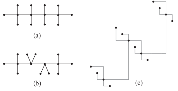
Figure 1: The ordered top-view caterpillar $C_{14}$ shown in (a) does not have a planar L-shaped drawing on the point set $P_{14}$ shown in (c). The ordering shown in (b) does.

Next we explore the question of how many points are needed for a planar L-shaped drawing of an $n$-vertex top-view caterpillar. Consider the appearance of the caterpillar’s spine (a path) in such a drawing. Each node of the spine, except for the two endpoints, must have its two incident spine edges aligned—both horizontal or both vertical. Define a straight-through drawing of a path to be a planar L-shaped drawing such that the two incident edges at each vertex are aligned. The best bound we have for the number of points that suffice for a straight-through drawing of a path is obtained when we draw the path in a monotone fashion, i.e. i.e. with non-decreasing x-coordinates.

Theorem 2.1

Any path of $n$ vertices has an $x$-monotone straight-through drawing on any set of at least $c\cdot n\log n$ points for some constant $c$.

Proof

We prove that if the number of points satisfies the recurrence $M(n)=2M(\frac{n}{2})+2n$ then any path of $n$ vertices has an $x$-monotone straight-through drawing on the points. Observe that this recurrence relation solves to $M(n)\in\Theta(n\log n)$ which will complete the proof. Within a constant factor we can assume without loss of generality that $n$ is a power of 2.

Order the points by $x$-coordinate. Recall our assumption that no two points share the same $x$- or $y$-coordinate. By induction, the first half of the path has an $x$-monotone straight-through drawing on the first $M(\frac{n}{2})$ points. We add the assumption that the path starts with a horizontal segment.

Let $p$ be the second last point used. Since $n$ is a power of 2, the path goes through $p$ on a horizontal segment. Let $T$ be the set of points to the right of and above $p$. Let $B$ be the set of points to the right of and below $p$. Refer to Figure 2(a). In $T$, consider the partial order $(x_{1},y_{1})\prec_{T}(x_{2},y_{2})$ if $x_{1}<x_{2}$ and $y_{1}<y_{2}$. Let $T^{\prime}$ be the set of minimal elements in this partial order. Similarly, in $B$, let $B^{\prime}$ be the set of elements that are minimal in the ordering $(x_{1},y_{1})\prec_{B}(x_{2},y_{2})$ if $x_{1}<x_{2}$ and $y_{1}>y_{2}$. If $T^{\prime}$ has $n$ or more points, then we can draw the whole path on $T^{\prime}$ with an $x$-monotone straight-through drawing starting with a horizontal segment. The same holds if $B^{\prime}$ has $n$ or more points. Thus we may assume that $|T^{\prime}|,|B^{\prime}|<n$. We now remove $T^{\prime}$ and $B^{\prime}$; let $R=(T-T^{\prime})\cup(B-B^{\prime})$. Then $|R|\geq M(\frac{n}{2})$.

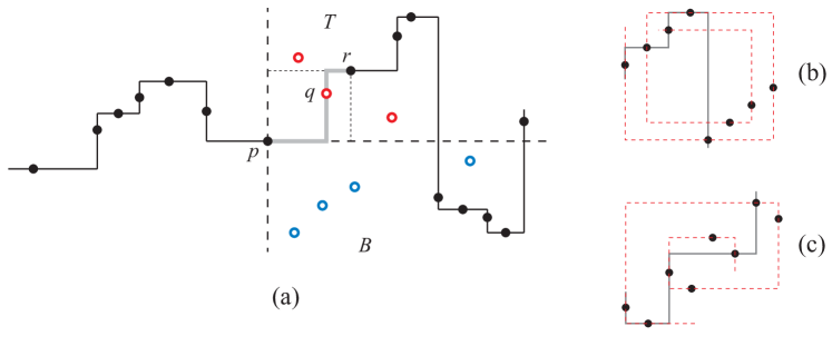
Figure 2: (a) The construction for the proof of Theorem 2.1. The points of $T^{\prime}$ and $B^{\prime}$ are drawn as hollow red points above $p$ and hollow blue points below $p$, respectively. (b-c) Examples of point sets of size $2n$ for which the maximum length of an $x$-monotone straight-through path is $n+1$. Such paths are shown in grey. In both cases there are non-monotone planar straight-through paths of length $2n$ (dashed).

By induction the second half of the path has an $x$-monotone straight-through drawing on the set $R$ starting with a horizontal segment. Let $r$ be the first point used for this drawing. Assume without loss of generality that $r$ lies in $T$. (The other case is symmetric.) Consider the rectangle with opposite corners at $p$ and $r$. Since $r$ is not in $T^{\prime}$, there is a point $q\in T$ inside the rectangle. We can join the two half paths using a vertical segment through $q$ and the last vertex of the first half path is embedded at $q$.

We can extend the above result to draw the entire caterpillar (not just its spine) with the same bound on the number of points:

Theorem 2.2

Any top-view caterpillar of $n$ vertices has a planar L-shaped drawing on any set of $c\cdot n\log n$ points for some constant $c$.

Proof (outline)

Follow the above construction, but in addition to $T^{\prime}$ and $B^{\prime}$, also take the second and third layers. If any layer has $n$ or more points, we embed the whole caterpillar on it [7]. Otherwise, we remove at most a linear number of points, and embed the second half of the caterpillar by induction on the remaining points. Then, in the rectangle between $p$ and $r$ there must be an increasing sequence of 3 points. Use the middle one for the left-over spine-vertex $q$ and the other two for the leaves of $q$.

We conjecture that $2n$ points suffice for an $x$-monotone straight-through drawing of any $n$-path. See Figure 2(b-c) for a lower bound of $2n$. Do $n$ points suffice if the $x$-monotone condition is relaxed to planarity? Finally, we mention that the problem of finding monotone straight-through paths is related to a problem about alternating runs in a sequence, as explained in Appendix 0.B.

3 Trees of Maximum Degree 3

In this section, we prove bounds on the number of points needed for L-shaped drawings of trees with maximum degree $3$. We treat the trees as rooted and thus, we refer to them as binary trees. We name the parts of the tree as shown in Figure 3(a). The root $r_{0}$ has two subtrees $T_{1}$ and $T_{2}$ of size $n_{1}$ and $n_{2}$, respectively, with $n_{1}\leq n_{2}$. $T_{2}$’s root, $r_{1}$, has subtrees of sizes $n_{2,1}$ and $n_{2,2}$ with $n_{2,1}\leq n_{2,2}$.

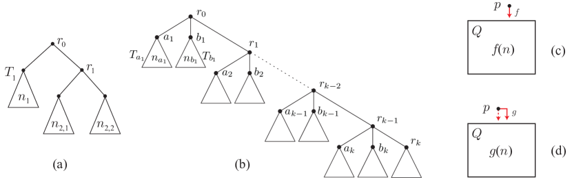
Figure 3: The naming conventions for (a) binary and (b) ternary trees. The set-up for (c) $f$-configurations and (d) $g$-configurations.

The main idea is to draw a tree $T$ on a set of points in a rectangle $Q$ by partitioning the rectangle into subrectangles in which we recursively draw subtrees. This gives rise to recurrence relations for the number of points needed to draw trees of size $n$, which we then analyze. We distinguish two subproblems or “configurations.” In each, we must draw a tree $T$ rooted at $r_{0}$ in a rectangle $Q$ that currently has no part of the drawing inside it. Furthermore, the parent $p$ of $r_{0}$ has already been drawn, and one or two rays outgoing from $p$ have been reserved for drawing the first segment of edge $(p,r_{0})$ (without hitting any previous part of the drawing).

In the $f$-configuration the reserved ray from $p$ goes vertically downward to $Q$. See Fig. 3(c). Let $f(n)$ be the smallest number of points such that any binary tree with $n$ vertices can be drawn in any rectangle with $f(n)-1$ points in the $f$-configuration. We will give various ways of drawing trees in the $f$-configuration, each of which gives an upper bound on $f(n)$. Among these choices, the algorithm uses the one that requires the fewest points.

In the $g$-configuration we reserve a horizontal ray from $p$, that allows the L-shaped edge $(p,r_{0})$ to turn downward into $Q$ at any point without hitting any previous part of the drawing. In addition, we reserve the vertical ray downward from $p$ in case this ray enters $Q$. See Fig. 3(d) for the case where the horizontal ray goes to the right. Let $g(n)$ be the smallest number of points such that any binary tree with $n$ vertices can be drawn in any rectangle with $g(n)-1$ points in the $g$-configuration. Observe that $f(n)\geq g(n)$ since the $g$-configuration gives us strictly more freedom.

We start with two easy constructions to give the flavour of our methods.

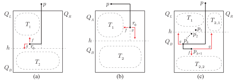
Figure 4: Three methods: (a) $f$-draw-1; (b) $g$-draw; and (c) $f$-draw-2.

$f$-draw-1. This method, illustrated in Figure 4(a), applies to an $f$-configuration. We first describe the construction and then say how many points are required. Continue the vertical ray from $p$ downward to a horizontal half-grid line $h$ determined as follows. Partition $Q$ by $h$ and the ray down to $h$ into 3 parts: $Q_{B}$, the rectangle below $h$; $Q_{L}$, the upper left rectangle; and $Q_{R}$, the upper right rectangle. Choose $h$ to be the highest half-grid line such that $Q_{L}$ or $Q_{R}$ has $f(n_{1})$ points. Without loss of generality, assume that $Q_{L}$ has $f(n_{1})$ points, and $Q_{R}$ has at most $f(n_{1})$ points. Place $r_{0}$ at the bottommost point of $Q_{L}$. Draw the edge $(p,r_{0})$ down and left. Start a ray vertically up from $r_{0}$, and recursively draw $T_{1}$ in $f$-configuration (rotated $180^{\circ}$) in the subrectangle of $Q_{L}$ above $r_{0}$, which has $f(n_{1})-1$ points. This leaves the leftward and downward rays free at $r_{0}$, so we can draw $T_{2}$ recursively in $g$-configuration in $Q_{B}$ so long as there are $g(n_{2})-1$ points. The total number of points required is $2f(n_{1})+g(n_{2})-1$. Recall that $f(n)$ is 1 more than the number of required points, so this proves:

$$f(n)\leq 2f(n_{1})+g(n_{2}). f$$ (-1)

Observe that we could have swapped $f$ and $g$ which proves:

$$f(n)\leq 2g(n_{1})+f(n_{2}). f$$ (-1’)

The above method can be viewed as a special case of Aichholzer et al.’s method for ternary trees [1] (see Section 4). We incorporate two new ideas to improve their result: first, they used only $f$-configurations, but we notice that one of the above two recursive subproblems is a $g$-configuration in the binary tree case, and can be solved by a better recursive algorithm; second, their method wasted all the points in $Q_{R}$, but we will give more involved constructions that allow us to use some of those points.

$g$-draw. This method applies to a $g$-configuration where the ray from the parent node $p$ goes to the right. Partition $Q$ at the highest horizontal half-grid line such that the top rectangle $Q_{A}$ has $f(n_{1})$ points. We separate into two cases depending whether the rightmost point, $q$, of $Q_{A}$ is to the right or left of $p$.

If $q$ is to the right of $p$, place $r_{0}$ at $q$, and draw the edge $(p,r_{0})$ right and down. See Figure 4(b). Start a ray leftward from $r_{0}$ and recursively draw $T_{1}$ in $f$-configuration in the subrectangle of $Q_{A}$ to the left of $q$. Note that there are $f(n_{1})-1$ points here, which is sufficient. The rightward and downward rays at $r_{0}$ are free, so we can draw $T_{2}$ recursively in $g$-configuration in $Q_{B}$ if there are $g(n_{2})-1$ points. The total number of points required is $f(n_{1})+g(n_{2})-1$.

If all points of $Q_{A}$ lie to the left of $p$, then place $r_{0}$ at the bottommost point of $Q_{A}$ and observe that we now have the situation of $f$-draw-1 with $Q_{R}$ empty, and $f(n_{1})+g(n_{2})-1$ points suffice.

This proves:

$$g(n)\leq f(n_{1})+g(n_{2}). g$$ ()

We now describe a different $f$-drawing method that is more efficient than $f$-draw-1 above, and will be the key for our bound for binary trees.

$f$-draw-2. This method applies to an $f$-configuration. We begin as in $f$-draw-1, though with the $f$-drawing and the $g$-drawing switched. Partition $Q$ by a horizontal half-grid line $h$ and the ray from $p$ down to $h$ into 3 parts: $Q_{B}$, the rectangle below $h$; $Q_{L}$, the upper left rectangle; and $Q_{R}$, the upper right rectangle. Choose $h$ to be the highest half-grid line such that $Q_{L}$ or $Q_{R}$ has $g(n_{1})$ points. Without loss of generality, assume the former. We separate into two cases depending on the size of $Q_{R}$.

If $|Q_{R}|<g(n_{2,1})$ then we follow the $f$-draw-1 method. Let $p_{1}$ be the bottommost point of $Q_{L}$. Place $r_{0}$ at $p_{1}$, draw the edge $(p,r_{0})$ down and left, recursively draw $T_{1}$ in $g$-configuration in $Q_{L}$ using leftward/upward rays from $r_{0}$, and recursively draw $T_{2}$ in $f$-configuration in $Q_{B}$ using a downward ray from $r_{0}$. This requires $g(n_{1})+g(n_{2,1})+f(n_{2})-1$ points, where $g(n_{2,1})$ accounts for the wasted points in $Q_{R}$.

If $|Q_{R}|\geq g(n_{2,1})$ then we make use of the points in $Q_{R}$ by drawing subtree $T_{2,1}$ there. Let $p_{1}$ be the bottommost point of $Q_{L}$, and let $p_{2},p_{3},\ldots$ be the points of $Q_{B}$ below $p_{1}$ in decreasing $y$-order. Let $k\geq 2$ be the smallest index such that either $k=n$ or point $p_{k+1}$ lies to the right of $p_{k}$. See Figure 4(c).

We have two subcases. If $k=n$, then $p_{1},\ldots,p_{k}$ form a monotone chain of length $n$, i.e., a diagonal point set in the terminology of Di Giacomo et al. [7]. They showed that any tree of $n$ points can be embedded on a diagonal point set, so we simply draw $T$ on these $n$ points. (Note that if this construction is used in the induction step, upward visibility is needed for connecting $T$ to the rest of the tree, and this can be achieved.)

Otherwise $k<n$. Place $r_{0}$ at point $p_{k}$ and $r_{1}$ at $p_{k+1}$. Draw the edge $(p,r_{0})$ down and left, and the edge $(r_{0},r_{1})$ down and right. Recursively draw $T_{1}$ in $g$-configuration in $Q_{L}$ using leftward/upward rays from $r_{0}$. Draw $T_{2,2}$ in $f$-configuration in the rectangle below $r_{1}$ using a downward ray from $r_{1}$. Draw $T_{2,1}$ in $g$-configuration in $Q_{R}$ using the rightward ray from $r_{1}$. Observe that if $r_{1}$ lies to the right of $p$ (i.e., below $Q_{R}$ rather than below $Q_{L}$) then the upward ray from $r_{1}$ is clear (as required for a $g$-drawing). The number of points required is at most $2g(n_{1})+n+f(n_{2,2})-1$. This accounts for at most $g(n_{1})$ points in $Q_{R}$, and at most $n$ points below $h$ and above $r_{1}$.

This proves:

$$f(n)\leq\max\{g(n_{1})+g(n_{2,1})+f(n_{2}),\ 2g(n_{1})+f(n_{2,2})+n\}. f$$ (-2)

Theorem 3.1

Any perfect binary tree with $n$ nodes has an L-shaped drawing on any point set of size $c\cdot n^{1.142}$ for some constant $c$.

Proof

For perfect binary trees we have $n_{1}=n_{2}=\frac{1}{2}n$ and $n_{2,1}=n_{2,2}=\frac{1}{4}n$. We solve the simultaneous recurrence relations for $f$ and $g$ in Appendix 0.C by induction.

Theorem 3.2

Any binary tree has an L-shaped drawing on any point set of size $c\cdot n^{1.22}$ for some constant $c$.

Proof

For $n_{1}\leq 0.349n$, we use recursion ($f$-1). For $n_{2,1}\leq 0.082n$, we combine recursion ($f$-1’) and ($f$-1) to obtain $f(n)\leq 2g(n_{1})+2f(n_{2,1})+g(n_{2,2})$. For $n_{1}>0.349n$ and $n_{2,1}>0.082n$, we use recursion ($f$-2). We solve the simultaneous recurrence relations for $f$ and $g$ in Appendix 0.D by induction.

4 Trees of Maximum Degree 4

In this section, we prove bounds on the number of points needed for L-shaped drawings of trees with maximum degree $4$. We treat the trees as rooted and refer to them as ternary trees. Given a ternary tree of $n$ nodes, let $a_{1}$, $b_{1}$ and $r_{1}$ be the three children of the root $r_{0}$. We use $T_{v}$ to denote the subtree rooted at a node $v$, and $n_{v}$ to denote the number of nodes in $T_{v}$. We name the children of the root such that $n_{a_{1}}\leq n_{b_{1}}\leq n_{r_{1}}$. For $i\geq 2$, let $a_{i},b_{i},r_{i}$ be the three children of $r_{i-1}$, named such that $n_{a_{i}}\leq n_{b_{i}}\leq n_{r_{i}}$. See Figure 3(b).

We will draw ternary trees using only the $f$-configuration as defined in Section 3 (see Figure 3(c)). In this section (as opposed to the previous one) we define $f(n)$ to be minimum number such that any ternary tree of $n$ nodes can be drawn in $f$-configuration on any set of $f(n)-1$ points.

As in Section 3, we will give various drawing methods, each of which gives a recurrence relation for $f(n)$. Then in Appendix 0.E we will analyze the recurrence relations. We begin with a re-description of Aichholzer et al.’s method [1].

$f_{4}$-draw-1. Extend the vertical ray from $p$ downward to a horizontal half-grid line $h$ determined as follows. Partition $Q$ by $h$ and the ray down to $h$ into 3 parts: $Q_{B}$, the rectangle below $h$; $Q_{L}$, the upper left rectangle; and $Q_{R}$, the upper right rectangle. Choose $h$ to be the highest half-grid line such that $Q_{L}$ or $Q_{R}$ has $2f(n_{a_{1}})+2f(n_{b_{1}})$ points. Without loss of generality, assume the former. Partition $Q_{L}$ vertically into two rectangles $Q_{LL}$ and $Q_{LR}$ with atleast $f(n_{a_{1}})$ points on the left and atleast $f(n_{b_{1}})$ points on the right respectively, with $Q_{LL}$ to the left of $Q_{LR}$. Place $r_{0}$ at the bottommost point in $Q_{LR}$. Extend a ray upward from $r_{0}$ and recursively draw $T_{b_{1}}$ on the remaining $f(n_{b_{1}})-1$ points in $Q_{LR}$. Extend a ray to the left from $r_{0}$ and recursively draw $T_{a_{1}}$ on the $f(n_{a_{1}})$ points in $Q_{LL}$. Finally, extend a ray downward from $r_{0}$ and recursively draw $T_{r_{1}}$ in $Q_{B}$. See Figure 5(a). The number of points required is $2f(n_{a_{1}})+2f(n_{b_{1}})+f(n_{r_{1}})-1$, so this proves:

$$f(n)\leq 2f(n_{a_{1}})+2f(n_{b_{1}})+f(n_{r_{1}}). f_{4}$$ (-1)

For example, in the case when $T$ is perfect (with $n_{a_{1}}=n_{b_{1}}=n_{r_{1}}=\tfrac{n}{3}$), the inequality ($f_{4}$-1) becomes $f(n)\leq 5f(n/3)$, which resolves to $O(n^{\log_{3}5})$ and $\log_{3}5\approx 1.465$. The critical case for this recursion, though, turns out to be when $n_{a_{1}}=0$ and $n_{b_{1}}=n_{r_{1}}=\tfrac{n}{2}$, which gives $f(n)\leq 3f(n/2)$ and leads to Aichholzer et al.’s $O(n^{\log_{3}2})$ result.

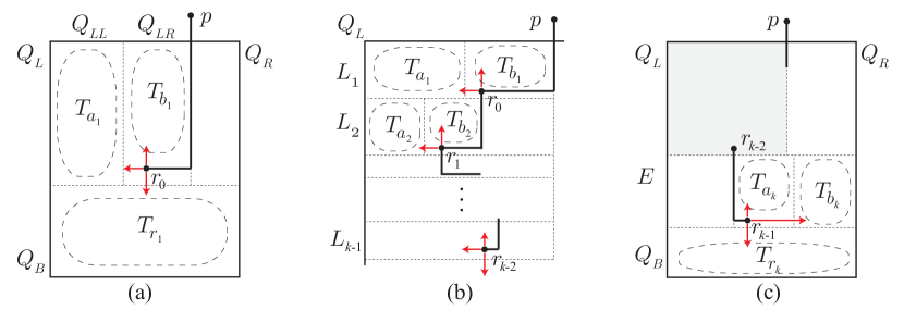
Figure 5: (a) $f_{4}$-draw-1. (b) Drawing the “small” subtrees in $Q_{L}$. (c) $f_{4}$-draw-2A.

$f_{4}$-draw-2. To improve their result, our idea again is to avoid wasting the points in $Q_{R}$, and use some of those points in the recursive drawings of subtrees at the next levels. However, simply considering subtrees at the second level is not sufficient for an asymptotic improvement if $T_{a_{2}}$ and $T_{b_{2}}$ are too small. Thus, we consider a more complicated approach that stops at the first level $k\geq 2$ where $n_{r_{k}}\leq 0.9n_{r_{k-1}}$. Note that for $i=2,\ldots,k-1$, we have $n_{r_{i}}>0.9n_{r_{i-1}}$ and $n_{a_{i}},n_{b_{i}}\leq 0.1n_{r_{i-1}}$, and so $T_{a_{i}}$ and $T_{b_{i}}$ are “small” subtrees. We apply the same idea as above to draw not just $T_{a_{1}},T_{b_{1}}$ but also all the small subtrees $T_{a_{i}}$ and $T_{b_{i}}$, $i=2,\ldots,k-1$ in $Q_{L}$ (appropriately defined), and then consider a few cases for how to draw the remaining “big” subtrees $T_{a_{k}},T_{b_{k}}$, and $T_{r_{k}}$, possibly using some points in $Q_{R}$. The number of points we will need to reserve for drawing $T_{a_{1}},T_{b_{1}},\ldots,T_{a_{k-1}},T_{b_{k-1}}$ is

$$Y=f(n_{a_{1}})+f(n_{b_{1}})+\sum_{i=2}^{k-1}(2f(n_{a_{i}})+2f(n_{b_{i}})).$$

Extend the vertical ray from $p$ downward until $Q_{L}$ or $Q_{R}$ has $Y$ points. Without loss of generality, assume the former.

Drawing the small subtrees. We draw nodes $r_{i}$ and subtrees $T_{a_{i}}$ and $T_{b_{i}}$, $i=1,\ldots,k-1$ in $Q_{L}$ as follows. Split $Q_{L}$ horizontally into rectangles $L_{1},\ldots,L_{k-1}$. The plan is to draw $r_{i},T_{a_{i}}$ and $T_{b_{i}}$ in $L_{i}$, in the same way that $T_{a_{1}}$ and $T_{b_{1}}$ were drawn in $f_{4}$-draw-1. See Figure 5(b). Level $L_{1}$ is special because the vertical ray from $p$ is at the right boundary of $L_{1}$. Thus, we require $f(n_{a_{1}})+f(n_{b_{1}})$ points. For levels $L_{i}$, $i=2,\ldots,k-1$ the vertical ray from $r_{i-2}$ may enter $L_{i}$ at any point, so we require $2f(n_{a_{i}})+2f(n_{b_{i}})$ points to follow the plan of $f_{4}$-draw-1, and the L-shaped edge from $r_{i-2}$ to $r_{i-1}$ may turn left or right. The total number of points we need in all levels is $Y$, which is why we defined $Y$ as we did.

Drawing the final three subtrees. It remains to draw $r_{k-1}$ and its three subtrees $T_{a_{k}}$, $T_{b_{k}}$, and $T_{r_{k}}$. We will draw $T_{r_{k}}$ on the bottommost $f(n_{r_{k}})-1$ points of $Q$. Call this rectangle $Q_{B}$. Let $E$ be the “equatorial zone” that lies between $Q_{L},Q_{R}$ above and $Q_{B}$ below. See Figure 5(c). If we are lucky, then not too many points are wasted in $Q_{R}$. Let $Z\leq Y$ be the number of points in $Q_{R}$.

Case A:

$Z<f(n_{b_{k}})$. In this case we draw $r_{k-1},T_{a_{k}}$ and $T_{b_{k}}$ in $E$ as in $f_{4}$-draw-1. See Figure 5(c). For this, we need $2f(n_{a_{k}})+2f(n_{b_{k}})$ points in $E$. The total number of points required in this case is $Y+Z+2f(n_{a_{k}})+2f(n_{b_{k}})+f(n_{r_{k}})-1$, so this proves:

$$f(n) \leq Y{+}Z{+}2f(n_{a_{k}}){+}2f(n_{b_{k}}){+}f(n_{r_{k}}) f_{4}$$ (-2A)

$$=f(n_{a_{1}}){+}f(n_{b_{1}}){+}\sum_{i=2}^{k-1}\left(2f(n_{a_{i}}){+}2f(n_{b_{i}})\right){+}2f(n_{a_{k}}){+}3f(n_{b_{k}}){+}f(n_{r_{k}}).$$

We must now deal with the unlucky case when $Z\geq f(n_{b_{k}})$. We will require $3f(n_{a_{k}})+f(n_{b_{k}})$ points in $E$. We sum up the total number of points below, but first we describe how to complete the drawing in $E$. Partition $E$ into three regions: $E_{L}$, $E_{M}$, and $E_{R}$, where $E_{L}$ is the region to the left of $r_{k-2}$, $E_{R}$ is the region to the right of $p$, and $E_{M}$ is the region between them. See Figure 6. Observe that either $|E_{L}|\geq f(n_{a_{k}})+f(n_{b_{k}})$, or $|E_{M}|\geq f(n_{a_{k}})$, or $|E_{R}|>f(n_{a_{k}})$. We show how to draw $r_{k-1},T_{a_{k}}$ and $T_{b_{k}}$ in each of these 3 cases.

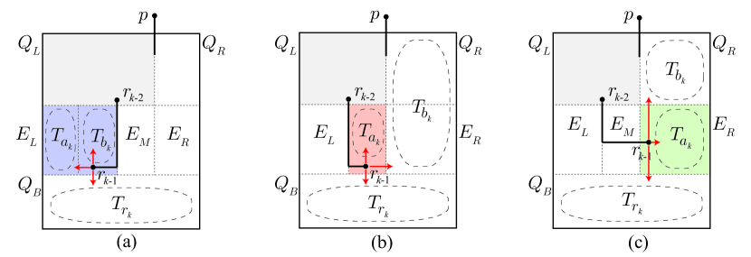
Figure 6: The drawings for $f_{4}$-draw-2B: (a) Case B1, with $E_{L}$ in blue; (b) Case B2, with $E_{M}$ in red; (c) Case B3, with $E_{R}$ in green.

Case B1:

$|E_{L}|\geq f({n_{a_{k}}})+f(n_{b_{k}})$. In this case we draw $r_{k-1},T_{a_{k}}$ and $T_{b_{k}}$ in $E_{L}$ as in $f_{4}$-draw-1. See Figure 6(a). Since $E_{L}$ is to the left of the ray down from $r_{k-2}$, we have sufficiently many points.

Case B2:

$|E_{M}|\geq f(n_{a_{k}})$. In this case we place $r_{k-1}$ at the lowest point of $E_{M}$, draw $T_{a_{k}}$ above it in $E_{M}$, and $T_{b_{k}}$ to its right in $Q_{R}\cup E_{R}$. See Figure 6(b). Since $|Q_{R}|=Z\geq f(n_{b_{k}})$, we have enough points to do this.

Case B3:

$|E_{R}|>f(n_{a_{k}})$. In this case we place $r_{k-1}$ at the leftmost point of $E_{R}$, draw $T_{a_{k}}$ to its right in $E_{R}$ and $T_{b_{k}}$ above it in $Q_{R}$. See Figure 6(c). Again, there are sufficiently many points.

The total number of points required in each of these three cases is $Y+Z+3f(n_{a_{k}})+f(n_{b_{k}})+f(n_{r_{k}})-1$, and $Y\leq Z$ which yields:

$$f(n) \leq Y+Z+3f(n_{a_{k}})+f(n_{b_{k}})+f(n_{r_{k}}) f_{4}$$ (-2B)

$$=2f(n_{a_{1}})+2f(n_{b_{1}})+\sum_{i=2}^{k-1}(4f(n_{a_{i}})+4f(n_{b_{i}}))+3f(n_{a_{k}})+f(n_{b_{k}})+f(n_{r_{k}}).$$

The bound on $f(n)$ obtained from $f_{4}$-draw-2 is the maximum of ($f_{4}$-2A) and ($f_{4}$-2B).

Theorem 4.1

Any ternary tree with $n$ nodes has an L-shaped drawing on any point set of size $2n^{1.55}$.

Proof

For $n_{b_{1}}\leq 0.47n$, we use recursion ($f_{4}$-1). Otherwise, we use ($f_{4}$-2A) or ($f_{4}$-2B) and take the larger of the two bounds. We solve the recurrence relation for $f$ in Appendix 0.E by induction.

5 Conclusions

We have made slight improvements on the exponent $t$ in the bounds that $c\cdot n^{t}$ points always suffice for drawing trees of maximum degree 4, or 3, with L-shaped edges. Improving the bounds to, e.g., $O(n\log n)$ will require a breakthrough. In the other direction, there is still no counterexample to the possibility that $n$ points suffice.

We introduced the problem of drawing ordered trees with L-shaped edges, where many questions remain open. For example: Do $c\cdot n$ points suffice for drawing ordered caterpillars? Can our isolated example be expanded to prove that $n$ points are not sufficient in general?

Acknowledgments We thank Jeffrey Shallit for investigating the alternating sequences discussed in Section 2. This work was done as part of a Problem Session in the Algorithms and Complexity group at the University of Waterloo. We thank the other participants for helpful discussions.

Appendix 0.A Proof of Lemma 1

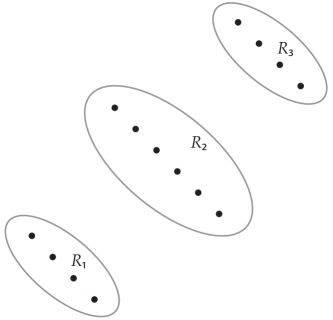
Figure 7: Point set $P_{14}$ of size $14$.

Let us denote the three groups of points by $R_{1}$, $R_{2}$ and $R_{3}$ as shown in Fig. 7. Let $s_{1},\dots,s_{4}$ be the spine-vertices (the vertices of degree 4 of $C_{14}$), in order along the spine. We prove Lemma 1 using the following two claims:

Claim

Let $r$ and $t$ be two points in $R_{i}$ for some $i\in\{1,2,3\}$ that are both assigned spine-vertices of $C_{14}$ such that $r$ is to the left of and above $t$. Then $r$ and $t$ are not consecutive in the $x$-order of points of $R_{i}$.

Proof

The bottom ray of $r$ must be used since spine-vertices have degree 4. If $r$ and $t$ are consecutive, then no point lies between them either in $x$-direction or in $y$-direction, which means that the bottom ray of $r$ either connects to $t$ or goes beyond the $y$-coordinate of $t$. Likewise the left ray of $t$ either connects to $r$ or goes beyond the $x$-coordinate of $r$, but the latter is impossible since then the bottom ray of $r$ would intersect the left ray of $t$. So $(r,t)$ exists and is routed along the bottom of $r$ and the left of $t$. Repeating the argument with the right ray of $r$ and the top ray of $t$ gives that $(r,t)$ is a double edge, a contradiction.

Claim

There is at most one spine-vertex in $R_{1}$, and it is either $s_{1}$ or $s_{4}$.

Proof

No vertex of degree 4 can be on the leftmost or bottommost point of $R_{1}$, since the left/bottom ray from it could not be used. The remaining two points cannot be both assigned to spine-vertices by Claim 0.A, so at most one spine-vertex belongs to $R_{1}$.

Now assume for contradiction that $s_{2}\in R_{1}$. By the order-constraints the edges $(s_{1},s_{2})$ and $(s_{2},s_{3})$ are both incident to $s_{2}$ vertically or both horizontally. Say they are both vertical, which means that one of $s_{1},s_{3}$ is lower down than $s_{2}$, and therefore also in $R_{1}$. This contradicts that only one spine-vertex belongs to $R_{1}$. Similarly we obtain a contradiction if both $(s_{1},s_{2})$ and $(s_{2},s_{3})$ are horizontal, so $s_{2}\not\in R_{1}$ and similarly $s_{3}\not\in R_{1}$.

Similarly neither $s_{2}$ nor $s_{3}$ are in $R_{3}$. We know that at most three spine-vertices are in $R_{2}$ by Claim 0.A, so at least one spine-vertex is in $R_{1}\cup R_{3}$, and it must be $s_{1}$ or $s_{4}$. Say $s_{1}\in R_{1}$ (all other cases are symmetric).

We may assume that edge $(s_{1},s_{2})$ leaves $s_{1}$ vertically, the other case is the same after a diagonal flip of the point set. Since $s_{2}\in R_{2}$, edge $(s_{1},s_{2})$ arrives at $s_{2}$ horizontally and from the left. So $(s_{2},s_{3})$ leaves $s_{3}$ horizontally to the right, and hence must go downward to reach $s_{3}$, because $s_{3}\in R_{2}$. So $(s_{2},s_{3})$ reaches $s_{3}$ from the top, which means that $(s_{3},s_{4})$ leaves $s_{3}$ from the bottom and $s_{4}\not\in R_{3}$. But also $s_{4}\not\in R_{1}$ since $s_{1}\in R_{1}$ and as argued above only one spine-vertex belongs to $R_{1}$. So $s_{4}\in R_{2}$ as well.

This means that the four points in $R_{3}$ are all used for leaves. There are only five leaves for which the corresponding edges could possibly reach $R_{3}$: the top ray from $s_{2}$, the right ray from $s_{3}$, the top and right ray from $s_{4}$, and the right ray from $s_{1}$. If both the right ray from $s_{3}$ and the top ray from $s_{4}$ go towards points in $R_{3}$ then they will intersect, contradicting planarity. Thus, not both of these can be using leaves in $R_{3}$, which means that the right ray from $s_{1}$ must go to $R_{3}$. But then the right ray from $s_{1}$ blocks any of the left/bottom rays from $s_{2},s_{3},s_{4}$ from reaching $R_{1}$. In consequence, only the rays from $R_{1}$ can reach leaves in $R_{1}$, leaving at least one point in $R_{1}$ unused. Contradiction, so $C_{14}$ has no embedding on $P_{14}$.

Appendix 0.B A Connection between Straight-through Drawings of Paths and Alternating Runs in Sequences

The problem of finding monotone straight-through paths is related to the following problem about alternating runs in a sequence. Given a sequence $s_{1}$, $s_{2},\ldots,s_{n}$, whose elements are a permutation of $1,\ldots,n$ find a maximum size set of indices $i_{1}\leq i_{2}\cdots\leq i_{k}$ such that the subsequence $s_{i_{1}},s_{i_{2}},\ldots,s_{i_{k}}$ is 3-good, meaning that it consists of alternating runs of length at least 3. A run is an increasing sequence or a decreasing sequence. For example, the subsequence $1,3,6,4,2,10,12,13$ is 3-good since its three runs, $1,3,6$ and $6,4,2$ and $2,10,12,13$ have lengths 3, 3, and 4 respectively. The subsequence $1,4,3$, $2,10,12,13$ is not 3-good because its first run, $1,4$ is too short.

The monotone straight-through drawing problem differs from the alternating runs problem in that the straight-through drawing problem requires all runs to be of odd length, but, on the other hand, tolerates shorter runs at the beginning and the end. For the alternating runs problem, it seems that a sequence of length $2n$ always has a 3-good subsequence of length $n$, except for the sequence $5,2,6,3,1,7,4$—this sequence has length 7, but its longest 3-good subsequence has length 3.

Appendix 0.C Analysis for Perfect Binary Trees

Proof (of Theorem 3.1)

For perfect binary trees we have $n_{1}=n_{2}=\frac{1}{2}n$ and $n_{2,1}=n_{2,2}=\frac{1}{4}n$. We use $\bar{f},\bar{g}$ for the functions in this special case. We claim that $\bar{g}(n)\leq\beta cn^{\alpha}$ and $\bar{f}(n)\leq cn^{\alpha}$, for $\alpha=1.142$, $\beta=1/(2^{\alpha}-1)\approx 0.8286$, and $c=24$. Clearly we have $\bar{g}(1)\leq\beta c$ and $\bar{f}(1)\leq c$ since one point is enough to draw the tree. Now assume that the bounds hold for all values $<n$. We apply $(g)$ and have

$$\bar{g}(n)\leq\bar{f}(\tfrac{1}{2}n)+\bar{g}(\tfrac{1}{2}n)\leq c(\tfrac{1}{2}n)^{\alpha}+\beta c\cdot(\tfrac{1}{2}n)^{\alpha}=\tfrac{1+\beta}{2^{\alpha}}cn^{\alpha}=\beta cn^{\alpha}$$

as desired (since $\beta$ is chosen so that $1+\beta=2^{\alpha}\beta$). For function $f$, the algorithm uses the best of the recursions, which means that it is no worse than recursion ($f$-2), and we have

$$\bar{f}(n) \leq \max\{2\bar{g}(\tfrac{1}{2}n)+\bar{f}(\tfrac{1}{4}n)+n,\,\bar{g}(\tfrac{1}{2}n)+\bar{g}(\tfrac{1}{4}n)+\bar{f}(\tfrac{1}{4}n)\}$$

$$\leq \max\{2\beta c(\tfrac{1}{2}n)^{\alpha}+c(\tfrac{1}{4}n)^{\alpha}+n^{\alpha},\,\beta c(\tfrac{1}{2}n)^{\alpha}+\beta c(\tfrac{1}{4}n)^{\alpha}+c(\tfrac{1}{4}n)^{\alpha}\}\leq cn^{\alpha}$$

since (with our choice of $\alpha,\beta,c$) we have

$$2\beta c(\tfrac{1}{2})^{\alpha}+c(\tfrac{1}{4})^{\alpha}+1<0.957c+1 <c\quad\text{and}$$

$$\beta c(\tfrac{1}{2})^{\alpha}+\beta c(\tfrac{1}{4})^{\alpha}+c(\tfrac{1}{4})^{\alpha}\leq 0.999c <c.$$

(A more careful analysis shows that the exponent in Theorem 3.1 approaches $\log_{2}x$ where $x$ is the real root of the cubic polynomial $x^{3}-2x^{2}-1=0$.)

Appendix 0.D Analysis for General Binary Trees

Proof (of Theorem 3.2)

We claim that $g(n)\leq\beta cn^{\alpha}$ and $f(n)\leq cn^{\alpha}$, for $\alpha=1.220$, $\beta=1/(2^{\alpha}-1)\approx 0.7522$, and $c=112$. Clearly we have $g(1)\leq\beta c$ and ${f}(1)\leq c$ since one point is enough to draw the tree. Now assume that the bound holds for all values $<n$ and consider the recursive formulas. As in the previous proof we have $g(n)\leq\beta cn^{\alpha}$ since $\beta=1/(2^{\alpha}-1)$.

As for $f$, the algorithm always uses the best-possible recursion, so it suffices (for various cases of how nodes are distributed in the subtrees) to argue that for one of the recursions we have $f(n)\leq cn^{\alpha}$.

• Case 1: $n_{1}\leq 0.349n$. We use recursion ($f$-1), i.e., $f(n)\leq 2g(n_{1})+f(n_{2})$. Applying induction, hence $f(n)\leq 2\beta cn_{1}^{\alpha}+cn_{2}^{\alpha}$. For this and the other cases, since the bivariate function $F(n_{1},n_{2})=2\beta cn_{1}^{\alpha}+cn_{2}^{\alpha}$ is convex over the domain $\{(n_{1},n_{2})\in[n]^{2}:n_{1}+n_{2}\leq n,\ n_{1}\leq 0.349n\}$, it suffices to check that the bound holds at the extreme points of the domain (see [12, Lemma 10]). The extreme points for $(n_{1},n_{2})$ in this case (ignoring the origin) are $(0,n)$ and $(0.349n,0.651n)$. For all of them we have $f(n)\leq cn^{\alpha}$ since

  $$2c(0)^{\alpha}+\beta c(n)^{\alpha}=\beta cn^{\alpha} <0.753cn^{\alpha}\quad\text{and}$$

  $$2c(0.349n)^{\alpha}+\beta c(0.651n)^{\alpha} <0.9993cn^{\alpha}.$$

• Case 2: $n_{2,1}\leq 0.082n$. We have $f(n)\leq 2g(n_{1})+f(n_{2})$ by ($f$-1’) and $f(n_{2})\leq 2f(n_{2,1})+g(n_{2,2})$ by ($f$-1), so $f(n)\leq 2g(n_{1})+2f(n_{2,1})+g(n_{2,2})\leq 2\beta cn_{1}^{\alpha}+2cn_{2,1}^{\alpha}+\beta cn_{2,2}^{\alpha}$. The extreme points for $(n_{1},n_{2,1},n_{2,2})$ are $(0,0,n)$, $(0,0.082n,0.918n)$, $(\frac{1}{2}n,0,\frac{1}{2}n)$, and $(\frac{1}{2}n,0.082n,0.418n)$. For all of them we have $f(n)\leq cn^{\alpha}$ since

  $$2\beta c(0)^{\alpha}+2c(0)^{\alpha}+\beta c(n)^{\alpha} < 0.753cn^{\alpha}$$

  $$2\beta c(0)^{\alpha}+2c(0.082n)^{\alpha}+\beta c(0.918n)^{\alpha} < 0.773cn^{\alpha}$$

  $$2\beta c(\tfrac{1}{2}n)^{\alpha}+2c(0)^{\alpha}+\beta c(\tfrac{1}{2}n)^{\alpha} < 0.969cn^{\alpha}$$

  $$2\beta c(\tfrac{1}{2}n)^{\alpha}+2c(0.082n)^{\alpha}+\beta c(0.418n)^{\alpha} < 0.99991cn^{\alpha}.$$

• Case 3: $n_{1}>0.349n$ and $n_{2,1}>0.082n$. Using recursion ($f$-2), we know that

  $$f(n) \leq\max\{g(n_{1})+g(n_{2,1})+f(n_{2}),\,2g(n_{1})+f(n_{2,2})+n\}$$

  $$\leq\max\{\beta cn_{1}^{\alpha}+\beta cn_{2,1}^{\alpha}+cn_{2},\,2\beta cn_{1}^{\alpha}+cn_{2,2}^{\alpha}+n^{\alpha}\}.$$

  The extreme points for $(n_{1},n_{2,1},n_{2})$ are $(\frac{1}{2}n,\frac{1}{4}n,\frac{1}{2}n)$ and $(0.349n,0.3255n,\allowbreak 0.651n)$ and the extreme points for $(n_{1},n_{2,2})$ are $(\frac{1}{2}n,0.418n)$ and $(0.349n,\allowbreak 0.569n)$. For all of them we have $f(n)\leq cn^{\alpha}$ since

  $$\beta c(\tfrac{1}{2}n)^{\alpha}+\beta c(\tfrac{1}{4}n)^{\alpha}+c(\tfrac{1}{2}n)^{\alpha} < 0.891cn^{\alpha}$$

  $$\beta c(0.349n)^{\alpha}+\beta c(0.322n)^{\alpha}+c(0.651n)^{\alpha} < 0.992cn^{\alpha}$$

  $$2\beta c(\tfrac{1}{2}n)^{\alpha}+c(0.418n)^{\alpha}+n^{\alpha} < (0.991c+1)n^{\alpha}<cn^{\alpha}$$

  $$2\beta c(0.349n)^{\alpha}+c(0.569n)^{\alpha}+n^{\alpha} < (0.920c+1)n^{\alpha}<cn^{\alpha}$$

  where the inequalities hold since we chose $c$ such that $0.991c+1<c$.

Appendix 0.E Analysis for Ternary Trees

Proof (of Theorem 4.1)

We will show by induction on $n$ that $f(n)\leq cn^{\alpha}$ for $\alpha=1.55$ and $c=2$. The bound holds for $n=1$ since one point is enough. Now assume that the bound holds for all values $<n$. We split the induction step into two cases based on the size of $T_{b_{1}}$. The algorithm uses the best-possible recursion, which means that it suffices to show that the bound holds for one of the recursive formulas for $f$.

• Case 1: $n_{b_{1}}\leq 0.47n$. By ($f_{4}$-1) and the induction hypothesis, we know $f(n)\leq 2c(n_{a_{1}})^{\alpha}+2c(n_{b_{1}})^{\alpha}+c(n_{r_{1}})^{\alpha}.$ Since the trivariate function $F(n_{a_{1}},n_{b_{1}},n_{r_{1}})=2(n_{a_{1}})^{\alpha}+2(n_{b_{1}})^{\alpha}+(n_{r_{1}})^{\alpha}$ is convex, it suffices to check whether the bound holds for the extreme points of the convex region $\{(n_{a_{1}},n_{b_{1}},n_{r_{1}})\in[0,n]^{3}:n_{a_{1}}+n_{b_{1}}+n_{r_{1}}\leq n,\ n_{a_{1}}\leq n_{b_{1}}\leq n_{r_{1}},\ n_{b_{1}}\leq 0.47n\}$. In this case, the extreme points (excluding the origin) are $(0,0,n)$, $(\tfrac{1}{3}n,\tfrac{1}{3}n,\tfrac{1}{3}n)$, and $(0,0.47n,0.53n)$. Since

  $$2(0)+2(0)+(n^{\alpha}) \leq n^{\alpha}$$

  $$2(\tfrac{1}{3}n)^{\alpha}+2(\tfrac{1}{3}n)^{\alpha}+(\tfrac{1}{3}n)^{\alpha} <0.911n^{\alpha}$$

  $$2(0)+2(0.47n)^{\alpha}+(0.53n)^{\alpha} <0.995n^{\alpha},$$

  we have $f(n)\leq cn^{\alpha}$ in this case.

• Case 2: $n_{b_{1}}>0.47n$. We know that $n_{r_{1}}<0.53n$ and therefore $n_{b_{k}}\leq n_{r_{k-1}}/2<0.265n$. By ($f_{4}$-2A) and ($f_{4}$-2B) and the induction hypothesis,

  $$f(n)\leq\max\left\{\begin{array}[]{l}c(n_{a_{1}})^{\alpha}+c(n_{b_{1}})^{\alpha}+\sum_{i=2}^{k-1}(2c(n_{a_{i}})^{\alpha}+2c(n_{b_{i}})^{\alpha})+{}\\ 2c(n_{a_{k}})^{\alpha}+3c(n_{b_{k}})^{\alpha}+c(n_{r_{k}})^{\alpha},\\[3.0pt] 2c(n_{a_{1}})^{\alpha}+2c(n_{b_{1}})^{\alpha}+\sum_{i=2}^{k-1}(4c(n_{a_{i}})^{\alpha}+4c(n_{b_{i}})^{\alpha})+{}\\ +3c(n_{a_{k}})^{\alpha}+c(n_{b_{k}})^{\alpha}+c(n_{r_{k}})^{\alpha}.\end{array}\right.$$

  The second term in the maximum dominates the first since $2(n_{b_{k}})^{\alpha}\leq 2(0.265n)^{\alpha}<(0.47n)^{\alpha}\leq(n_{b_{1}})^{\alpha}$ for our choice of $\alpha=1.55$. To show that the second term is at most $cn^{\alpha}$, we use three intermediate claims and show

  $$2(n_{a_{1}})^{\alpha}{+}2(n_{b_{1}})^{\alpha}{+}\textstyle{\sum_{i=2}^{k-1}}(4(n_{a_{i}})^{\alpha}{+}4(n_{b_{i}})^{\alpha}){+}3(n_{a_{k}})^{\alpha}{+}(n_{b_{k}})^{\alpha}{+}(n_{r_{k}})^{\alpha}\$$

  $$\leq 2(n_{a_{1}})^{\alpha}{+}2(n_{b_{1}})^{\alpha}{+}\textstyle{\sum_{i=2}^{k-1}}(4(n_{a_{i}})^{\alpha}{+}4(n_{b_{i}})^{\alpha}){+}0.92(n_{r_{k-1}})^{\alpha}\quad\text{(by Claim \ref{claim1})}$$

  $$\leq 2(n_{a_{1}})^{\alpha}{+}2(n_{b_{1}})^{\alpha}{+}0.92(n_{r_{1}})^{\alpha}\quad\text{(by Claim \ref{claim2} for $j=k{-}1,\dots,2$)}$$

  $$\leq n^{\alpha}\quad\text{(by Claim \ref{claim3}).}$$

  The three claims are proved as follows:

  Claim

  $3(n_{a_{k}})^{\alpha}+(n_{b_{k}})^{\alpha}+(n_{r_{k}})^{\alpha}<0.92(n_{r_{k-1}})^{\alpha}$.

  We can check that the claim holds by calculating the values for the extreme points of the region defined by our constraints, viz., $\{(n_{a_{k}},n_{b_{k}},n_{r_{k}})\in[0,n]^{3}:\allowbreak n_{a_{k}}{+}n_{b_{k}}{+}n_{r_{k}}\leq n_{r_{k-1}},\ n_{a_{k}}\leq n_{b_{k}}\leq n_{r_{k}}\leq 0.9n_{r_{k-1}}\}$. These are the points $(0,\frac{n_{r_{k-1}}}{2},\frac{n_{r_{k-1}}}{2}),(0,0.1n_{r_{k-1}},\allowbreak 0.9n_{r_{k-1}}),(0.05n_{r_{k-1}},0.05n_{r_{k-1}},\allowbreak 0.9n_{r_{k-1}})$, and $(\tfrac{1}{3}n_{r_{k-1}},\tfrac{1}{3}n_{r_{k-1}},\tfrac{1}{3}n_{r_{k-1}})$, and we verify:

  $$0+\big{(}\tfrac{1}{2}n_{r_{k-1}}\big{)}^{\alpha}+\big{(}\tfrac{1}{2}n_{r_{k-1}}\big{)}^{\alpha}<0.685n_{r_{k-1}}^{\alpha}$$

  $$0+(0.1n_{r_{k-1}})^{\alpha}+(0.9n_{r_{k-1}})^{\alpha}<0.878n_{r_{k-1}}^{\alpha}$$

  $$3(0.05n_{r_{k-1}})^{\alpha}+(0.05n_{r_{k-1}})^{\alpha}+(0.9n_{r_{k-1}})^{\alpha}<0.888n_{r_{k-1}}^{\alpha}$$

  $$3\big{(}\tfrac{1}{3}n_{r_{k-1}}\big{)}^{\alpha}+\big{(}\tfrac{1}{3}n_{r_{k-1}}\big{)}^{\alpha}+\big{(}\tfrac{1}{3}n_{r_{k-1}}\big{)}^{\alpha}<0.911n_{r_{k-1}}^{\alpha}.$$

  Claim

  $4(n_{a_{j}})^{\alpha}+4(n_{b_{j}})^{\alpha}+0.92(n_{r_{j}})^{\alpha}<0.92(n_{r_{j-1}})^{\alpha}$ for $2\leq j\leq k-1$.

  We can check that the claim holds by calculating the values for the extreme points of the region $\{(n_{a_{j}},n_{b_{j}},n_{r_{j}})\in[0,n]^{3}:n_{a_{j}}{+}n_{b_{j}}{+}n_{r_{j}}\leq n_{r_{j-1}},\ n_{a_{k}}\leq n_{b_{k}}\leq n_{r_{k}}\leq 0.9n_{r_{j-1}}\}$, specifically, the points $(0,\tfrac{n_{r_{j-1}}}{2},\tfrac{n_{r_{j-1}}}{2})$, $(0,0.1n_{r_{j-1}},\allowbreak 0.9n_{r_{j-1}})$, $(0.05n_{r_{j-1}},0.05n_{r_{j-1}},0.9n_{r_{j-1}})$, and $(\tfrac{n_{r_{j-1}}}{3},\tfrac{n_{r_{j-1}}}{3},\tfrac{n_{r_{j-1}}}{3})$:

  $$0+0+0.92(n_{r_{k-2}})^{\alpha} <0.92(n_{r_{k-2}})^{\alpha}$$

  $$0+4(0.1n_{r_{k-2}})^{\alpha}+0.92(0.9n_{r_{k-2}})^{\alpha} <0.895(n_{r_{k-2}})^{\alpha}$$

  $$4(0.05n_{r_{k-2}})^{\alpha}+4(0.05n_{r_{k-2}})^{\alpha}+0.92(0.9n_{r_{k-2}})^{\alpha} <0.859(n_{r_{k-2}})^{\alpha}.$$

  Claim

  $2(n_{a_{1}})^{\alpha}+2(n_{b_{1}})^{\alpha}+0.92(n_{r_{1}})^{\alpha}\leq n^{\alpha}$.

  We can check that the claim holds by calculating the values for the extreme points of the region $\{(n_{a_{1}},n_{b_{1}},n_{r_{1}})\in[0,n]^{3}:n_{a_{1}}+n_{b_{1}}+n_{r_{1}}\leq n,\ n_{a_{1}}\leq n_{b_{1}}\leq n_{r_{1}},n_{b_{1}}>0.47n\}$, specifically, the points $(0.08n,0.47n,0.47n)$, $(0,\tfrac{1}{2}n,\tfrac{1}{2}n)$ and $(0,0,n)$:

  $$2(0.08n)^{\alpha}+2(0.47n)^{\alpha}+0.92(0.47n)^{\alpha} <0.946n^{\alpha}$$

  $$0+2(\tfrac{1}{2}n)^{\alpha}+0.92(\tfrac{1}{2}n)^{\alpha} <0.998n^{\alpha}$$

  $$0+0+0.92(n)^{\alpha} <0.92n^{\alpha}.$$

This finishes the proof of Theorem 4.1.

References

- [1] Aichholzer, O., Hackl, T., Scheucher, M.: Planar L-shaped point set embeddings of trees. In: European Workshop on Computational Geometry (EuroCG) (2016), Book of abstracts available at http://www.eurocg2016.usi.ch/
- [2] Bárány, I., Buchin, K., Hoffmann, M., Liebenau, A.: An improved bound for orthogeodesic point set embeddings of trees. In: European Workshop on Computational Geometry (EuroCG) (2016), Book of abstracts available at http://www.eurocg2016.usi.ch/
- [3] Bose, P.: On embedding an outer-planar graph in a point set. Computational Geometry 23(3), 303–312 (2002)
- [4] Bose, P., McAllister, M., Snoeyink, J.: Optimal algorithms to embed trees in a point set. Journal of Graph Algorithms and Applications 1(2), 1–15 (1997)
- [5] Cabello, S.: Planar embeddability of the vertices of a graph using a fixed point set is NP-hard. Journal of Graph Algorithms and Applications 10(2), 353–363 (2006)
- [6] Chrobak, M., Karloff, H.: A lower bound on the size of universal sets for planar graphs. ACM SIGACT News 20(4), 83–86 (1989)
- [7] Di Giacomo, E., Frati, F., Fulek, R., Grilli, L., Krug, M.: Orthogeodesic point-set embedding of trees. Computational Geometry 46(8), 929–944 (2013)
- [8] Fraysseix, H.d., Pach, J., Pollack, R.: How to draw a planar graph on a grid. Combinatorica 10(1), 41–51 (1990)
- [9] Gritzmann, P., Mohar, B., Pach, J., Pollack, R.: Embedding a planar triangulation with vertices at specified points. American Mathematical Monthly 98, 165–166 (1991)
- [10] Katz, B., Krug, M., Rutter, I., Wolff, A.: Manhattan-geodesic embedding of planar graphs. In: Eppstein, D., Gansner, E.R. (eds.) International Symposium on Graph Drawing (GD 2009). LNCS, vol. 5849, pp. 207–218. Springer (2009)
- [11] Kaufmann, M., Wiese, R.: Embedding vertices at points: Few bends suffice for planar graphs. Journal of Graph Algorithms and Applications 6(1), 115–129 (2002)
- [12] Scheucher, M.: Orthogeodesic point set embeddings of outerplanar graphs. Master’s thesis, Graz University of Technology (2015)
- [13] Schnyder, W.: Embedding planar graphs on the grid. In: Proceedings of the First ACM-SIAM Symposium on Discrete Algorithms (SODA). pp. 138–148 (1990)