ML and Near-ML Decoding of LDPC Codes Over the BEC: Bounds and Decoding Algorithms

Abstract

The performance of the maximum-likelihood (ML) decoding on the binary erasure channel for finite-length low-density parity-check (LDPC) codes from two random ensembles is studied. The theoretical average spectrum of the Gallager ensemble is computed by using a recurrent procedure and compared to the empirically found average spectrum for the same ensemble as well as to the empirical average spectrum of the Richardson-Urbanke ensemble and spectra of selected codes from both ensembles. Distance properties of the random codes from the Gallager ensemble are discussed. A tightened union-type upper bound on the ML decoding error probability based on the precise coefficients of the average spectrum is presented. A new upper bound on the ML decoding performance of LDPC codes from the Gallager ensemble based on computing the rank of submatrices of the code parity-check matrix is derived. A new lower bound on the ML decoding threshold followed from the latter error probability bound is obtained. An improved lower bound on the error probability for codes with known estimate on the minimum distance is presented as well. A new low-complexity near-ML decoding algorithm for quasi-cyclic LDPC codes is proposed and simulated. Its performance is compared to the simulated BP decoding performance and simulated performance of the best known improved iterative decoding techniques, as well as, with the upper bounds on the ML decoding performance and decoding thresholds obtained by the density evolution technique.

I Introduction

A binary erasure channel (BEC) is one of the simplest to analyze and consequently a well-studied communication channel model. In spite of its simplicity, during the last decades the BEC has started to play a more important role due to the emergence of new applications. For example, in communication networks virtually all errors occurring at the physical level can be detected using a rather small redundancy. Data packets with detected errors can be viewed as symbol erasures.

The analysis of the decoding performance on the BEC is simpler than for other channel models. On the other hand, it is expected that ideas and findings for the BEC might be useful for constructing codes and developing decoding algorithms for other important communication channels, such as, for example, the binary symmetric channel (BSC) or the additive white Gaussian noise (AWGN) channel.

A commonly used approach to the analysis of decoding algorithms is to study the performance of the algorithm applied to random linear codes over a given channel model. Two of the most studied code ensembles are the classical Gallager ensemble [3] and the more general ensemble presented in [4]. The Gallager ensemble is historically the first thoroughly studied ensemble of regular LDPC codes. The ensemble in [4] can be described by random Tanner graphs with given parity-check and symbol node degree distributions. We will refer to this ensemble and the LDPC codes contained in it as the Richardson-Urbanke (RU) ensemble and RU LDPC codes, respectively. These and some other ensembles of regular LDPC codes are described and analyzed in [5].

It is shown in [3, Appendix B] that the asymptotic weight enumerator of random $(J,K)$-regular LDPC codes approaches the asymptotic weight enumerator of random linear codes when $J$ and $K$ grow. In [5], it is confirmed that other ensembles of regular LDPC codes demonstrate a similar behavior. Thus, regular ensembles are good enough to achieve near-optimal performance. On the other hand, it is well-known that both asymptotically [4] and in a finite-length regime irregular LDPC codes outperform their regular counterparts and more often are recommended for real-life applications [6, 7]. Finite-length analysis of RU LDPC codes under belief propagation (BP) and (to a lesser degree) under maximum-likelihood (ML) decoding was performed in [8]. In this paper, we extend the analysis of the ML decoding case for regular codes. In particular, new error probability bounds for regular codes are presented. For general linear codes, detailed overviews of lower and upper bounds for the AWGN channel and the BSC were presented by Sason and Shamai in their tutorial paper [9], and for the AWGN channel, the BSC, and the BEC by Polyanskiy et al. in [10] and by Di et al. in [8].

For computing upper bounds on the error probability for LDPC codes there exist two approaches. One, more general, approach is based on a union-type bound and requires knowledge of the code weight enumerator or its estimate. The second approach used in [8] is suitable for the BEC. It implies estimating the rank of submatrices of the LDPC code parity-check matrix. Notice that for infinitely long codes, the bit error rate (BER) performance of BP decoding can be analyzed through density evolution (see e.g. [11, 4]). However, the density evolution technique is not suitable for analysis of finite-length codes, since dependencies caused by cycles in the Tanner graph associated with the code are not taken into account.

In this paper, first we consider a tightened union-type bound based on precise average spectra of random finite-length LDPC codes. The difference between our approach and other techniques is the way of computing the bound. Instead of manipulating with hardly computable coefficients of series expansions of generating functions, we compute the spectra by using efficient recurrent procedures. This allows for obtaining precise average weight enumerators with complexity growing linearly with the code length. New bounds, based on computing the rank of submatrices, are derived for the RU and the Gallager ensemble of regular LDPC codes. A tightened lower bound on the ML decoding error probability on the BEC, which is applicable to any linear code with a known upper bound on the minimum distance, is presented. For LDPC codes of short length, it shows a surprisingly strong improvement over the best known lower bound. A lower bound on the ML decoding threshold which stems from the derived upper rank-type bounds is derived. Notice that this bound obtained from the bound on the average block error probability over the Gallager and RU ensembles slightly differs from the ML decoding thresholds in [12] and [13] obtained from the bounds on the bit error probability of the average code in the RU ensemble.

A remarkable property of the BEC is that ML decoding of any linear code over this channel is reduced to solving a system of linear equations. This means that ML decoding of an $[n,k]$ LDPC code (where $n$ is the code length and $k$ is the number of information symbols) with $\nu$ erasures can be performed by Gaussian elimination with time complexity at most $O(\nu^{3})$. Exploiting the sparsity of the parity-check matrix of the LDPC codes can lower the complexity to approximately $O(\nu^{2})$ (see overview and analysis in [14] and references therein). Practically feasible algorithms with a thorough complexity analysis can be found in [15, 16, 17]. This makes ML-decoded LDPC codes strong competitors for scenarios with strong restrictions on the decoding delay. It is worth noting that ML decoding allows for achieving low error probability at rates strictly above the so-called BP decoding threshold [4]. However, ML decoding of long LDPC codes of lengths of tens of thousands of bits over the BEC is still considered impractical unless the code rate $R$ tends to $1$ or number of erasures is small (see, for example,[17]).

Low-complexity suboptimal decoding techniques for LDPC codes over the BEC are based on the following two approaches. The first approach consists of adding redundant rows to the original code parity-check matrix (see, for example, [18, 19, 20]). The second approach applies post-processing in case of BP decoding failure [21, 22, 23, 24]. In [21, 24], a post-processing step based on the concept of guessing bits is proposed. Applying bit guessing based algorithms to the decoding of LDPC codes improves the performance of BP decoding, but does not provide near-ML performance.

In this paper, we propose a new decoding algorithm which provides near-ML decoding of long quasi-cyclic (QC) LDPC block codes. It is well-known that QC LDPC codes are considered practical in terms of implementation complexity and they are often referred to as candidates for different communication standards. Furthermore, QC LDPC block codes can be represented as a tail-biting (TB) parent convolutional LDPC code. Thereby, decoding techniques developed for TB codes are applicable to QC LDPC codes. The proposed algorithm resembles a wrap-around suboptimal decoding of TB convolutional codes [25, 26]. Decoding of a TB code requires identification of the correct starting state, and thus ML decoding must apply the Viterbi algorithm once for each possible starting state. In contrast, wrap-around decoding applies the Viterbi algorithm once to the wrapped-around trellis diagram with all starting state metrics initialized to zero. This decoding approach yields near-ML performance at a typical complexity of a few times the complexity of the Viterbi algorithm.

The new algorithm belongs to a family of so-called hybrid decoding algorithms. It is based on a combination of BP decoding of the QC LDPC code followed by so-called “quasi-cyclic sliding-window” ML decoding. The latter technique is applied “quasi-cyclically” to a relatively short sliding window, where the decoder performs ML decoding of a zero-tail terminated (ZT) LDPC convolutional code. Notice that unlike sliding-window near-ML (SWML) decoding of convolutional codes considered in [27], the suggested algorithm working on the parent LDPC convolutional code has significantly lower computational complexity due to the sparsity of the code parity-check matrix [28]. On the other hand, it preserves almost all advantages of the convolutional structure in the sense of erasure correcting capability.

The rest of the paper is organized as follows. Preliminaries are given in Section II. A recurrent algorithm for computing the average spectrum for the Gallager ensemble of binary LDPC codes is presented in Section III. Empirical average spectra for the Gallager and RU ensembles are computed and compared to the theoretical average spectra as well as to the spectra of selected codes in the same section. Distance properties of the Gallager ensemble are discussed in Appendix A. In Section IV, an improved lower bound and two upper bounds on the error probability of ML decoding over the BEC are derived. The corresponding proofs are given in Appendices B and C for the RU and the Gallager ensemble, respectively. A new algorithm for near-ML decoding of long QC LDPC codes based on the interpretation of these codes as TB convolutional codes and using wrap-around sliding-window decoding is proposed in Section V. Simulation results confirm the efficiency of the algorithm and are presented in Section VI, while asymptotic decoding thresholds which stem from the derived rank bounds are computed in Section VII. Conclusions are drawn in Section VIII.

II Preliminaries

A binary linear $[n,k]$ code $\mathcal{C}$ of rate $R=k/n$ can be defined as the null space of a $r\times n$ binary parity-check matrix $H$ of rank $\rho=n-k\leq r$. Denote by $\{A_{n,w}\}$, $w=0,1,\dotsc,n$, the code weight enumerator, where $A_{n,w}$ is the number of codewords of weight $w$. By some abuse of notation, we use $A_{n,w}$ for both the weight enumerator of a specific code and for random weight enumerators in code ensembles.

Random parity-check matrices $H$ of size $r\times n$ do not necessarily have rank $\rho=r$ which means that in general $k\geq n-r$. Following a commonly accepted assumption we assume that $\rho=r$ when deriving bounds on the error probability, but we take the difference into account when considering code examples.

Two ensembles of random regular LDPC codes are studied below. The first ensemble is the Gallager ensemble [3] of $(J,K)$-regular LDPC codes. Codes of this ensemble are determined by random parity-check matrices $H$ which consist of strips $H_{i}$ of width $M=r/J$ rows each, $i=1,2,\dots,J$. All strips are random column permutations of the strip where the $j$-th row contains $K$ ones in positions $(j-1)K+1,(j-1)K+2,\ldots,jK$, for $j=1,2,\ldots,n/K$. The second ensemble is a special case of the ensemble described in [4, Definition 3.15]. Notice that the Gallager ensemble and the RU ensemble are denoted by $\mathcal{B}$ and $\mathcal{H}$, respectively, in [5].

For $a\in\{1,2,\dotsc\}$ denote by $a^{m}$ the sequence $(a,a,\dotsc,a)$ of $m$ identical symbols $a$. In order to construct an $r\times n$ parity-check matrix $H$ of an LDPC code from the RU ensemble perform the following steps.

• Construct the sequence $\bm{a}=(1^{J},2^{J},\dotsc,n^{J})$; and

• apply a random permutation $\pi(\cdot)$ to obtain a sequence $\bm{b}=\pi(\bm{a})=(b_{1},\dotsc,b_{N})$, where $N=Kr=Jn$. The elements $b_{1},\dotsc,b_{K}$ show the locations of the nonzero elements of the first row of $H$, elements $b_{K+1},\dotsc,b_{2K}$ show the locations of the nonzero elements of the second row of $H$, etc.

A code from the RU ensemble is $(J,K)$-regular if for a given permutation $\pi$ all elements of subsequences $(b_{iK-K+1},\dotsc,b_{iK})$ are different for all $i=1,\dotsc,r$, otherwise it is irregular. The regular RU codes belong to the ensemble $\mathcal{A}$ in [5] which is defined as the sub-ensemble of the RU ensemble containing the parity-check matrices with row weight $K$ and column weight $J$. It is shown in [5] that the three ensembles $\mathcal{A}$, $\mathcal{B}$, and $\mathcal{H}$ have the same asymptotic average weight enumerators.

It is known (see [5, Theorem 3]) that for large $n$ the total number of $(J,K)$-regular $[n,n-r]$ codes (ensemble $\mathcal{A}$ in [5]) is equal to

$$\frac{(Jn)!}{(K!)^{r}(J!)^{n}}\exp\left\{-\frac{(K-1)(J-1)}{2}\right\}\left(1+o(n^{-1+\delta})\right)\;,$$

where $\delta>0$ and $o(x)\to 0$ when $x\to 0$. The number of different codes from the RU ensemble constructed as described above is

$$\frac{(Jn)!}{(K!)^{r}(J!)^{n}}\;.$$

Thus, the portion of $(J,K)$-regular LDPC codes in the RU ensemble is

$$\exp\left\{-\frac{(K-1)(J-1)}{2}\right\}\left(1+o(n^{-1+\delta})\right)\;,$$

that is, most of the “$(J,K)$-regular” RU codes are indeed irregular. However, for a particular parity-check matrix, the fraction of rows of weight less than $K$ as well as the fraction of columns of weight less than $J$ is small (both fractions tend to zero when $n$ grows). Thus, this irregularity can be safely ignored. In the following, a code from the RU ensemble with parameters $J$ and $K$ will sometimes be referred to as a $(J,K)$-RU code or simply as a $(J,K)$-regular code even if it is not strictly $(J,K)$-regular. Also, with some abuse of language a $(J,K)$-regular code from the Gallager ensemble will be referred to as a $(J,K)$-Gallager code.

As a performance measure we use the word (block, frame) error rate (FER) $P_{e}$, which for the BEC is defined as the probability that the decoder cannot recover the information of a received word uniquely.

Consider ML decoding over the BEC, where $\varepsilon>0$ denotes the channel symbol erasure probability. Assume that a codeword $\bm{x}=(x_{1},\dotsc,x_{n})$ is transmitted and that $\nu$ erasures occurred. Then, we denote by $I$ the set of indices of the erased positions, that is, $I=\{i_{1},\dotsc,i_{\nu}\}\subseteq\{1,2,\dotsc,n\}$, $|I|=\nu$, and by $\bm{x}_{I}=(x_{i_{1}},\dotsc,x_{i_{\nu}})$ a vector of unknowns corresponding to the erased positions. Let $I^{\rm c}=\{1,2,\dotsc,n\}\setminus I$ and $\bm{x}_{I^{\rm c}}$ be the set of indices of unerased positions and the vector of unerased values of $\bm{x}$, respectively. Also, let $H_{I}$ be the submatrix of $H$ consisting of the columns indexed by $I$. From $\bm{x}H^{\rm T}=\bm{0}$, where $(\cdot)^{\rm T}$ denotes the transpose of its argument, it follows that

$$\bm{x}_{I}H_{I}^{\rm T}=\bm{x}_{I^{\rm c}}H_{I^{\rm c}}^{\rm T}\triangleq{\bm{s}}\;,$$ (1)

where $\bm{s}$ is the syndrome vector or, equivalently,

$$\bm{y}_{I}H_{I}^{\rm T}=\bm{0}\;,$$ (2)

where $\bm{y}=\bm{x}+\bm{x}^{\prime}$ is a codeword. If the solution of (2) is not unique, that is,

$$\mbox{rank}\left(H_{I}\right)<|I|\;,$$

where $\mbox{rank}\left(\cdot\right)$ denotes the matrix rank of its argument, then the corresponding set of erasures cannot be (uniquely) corrected. Otherwise, the set of erasures $I$ is correctable. Thus, the ML decoding error probability (for the BEC) is the probability of such a set $I$, that is,

$$P_{e}=\Pr\left(\mbox{rank}\left(H_{I}\right)<|I|\right)\;.$$ (3)

III Average spectra for ensembles of regular LDPC codes

III-A Weight enumerator generating functions

In this section, we study average weight enumerators for different ensembles of LDPC codes. The weight distribution of any linear code can be represented in terms of its weight generating function

$${G_{n}(s)=\sum_{w=0}^{n}A_{n,w}s^{w}\;,}$$

where $A_{n,w}$ is the random variable representing the number of binary codewords of weight $w$ and length $n$, and $s$ is a formal variable. Our goal is to find ${\rm E}\{A_{n,w}\}$, where $\rm E\{\cdot\}$ denotes the expected value over the code ensemble. In general, computing the coefficients ${\rm E}\{A_{n,w}\}$ is a rather difficult task. If a generating function can be represented as a degree of another generating function (or expressed via a degree of such a function), then for numerical computations we can use the following simple recursion.

Lemma 1:

Let $f(s)=\sum_{l\geq 0}f_{l}s^{l}$ be a generating function. Then, the coefficients in the series expansion of the generating function $F_{L}(s)=\left[f(s)\right]^{L}=\sum_{l\geq 0}F_{l,L}s^{l}$ satisfy the following recurrent equation

$$F_{l,L}=\left\{\begin{array}[]{ll}f_{l},&L=1\\ \sum_{i=0}^{l}f_{i}F_{l-i,L-1},&L>1\end{array}\right.\;.$$

III-B General linear codes

For completeness, we present the average spectrum for the ensemble of random linear codes determined by equiprobable $r\times n$ parity-check matrices, where $r=n-k$, and $k$ and $n$ are the code dimension and length, respectively. The weight generating function of all binary sequences of length $n$ is $G_{n}(s)=(1+s)^{n}$. Then, the average spectrum coefficients are

$${\rm E}\{A_{n,w}\}=\binom{n}{w}2^{-r}\;,\;w>0\;,$$ (5)

where $2^{-r}$ is the probability that a binary sequence $\bm{x}$ of length $n$ and weight $w>0$ satisfies $\bm{x}H^{\rm T}=\bm{0}$.

If a random linear code contains only codewords of even weight, then its generating function has the form

$$G_{n}(s)=\sum_{w\;\rm{even}}\binom{n}{w}s^{w}=\frac{(1+s)^{n}+(1-s)^{n}}{2}\;,$$

and the average spectrum coefficients are

$${\rm E}\{A_{n,w}\}=\left\{\begin{array}[]{ll}2^{-r+1}\binom{n}{w},&w>0\mbox{ and even}\\ 0,&w\mbox{ odd}\end{array}\right.\;.$$ (6)

III-C The Gallager binary $(J,K)$-regular random LDPC codes

The generating function of the number of sequences satisfying the nonzero part of one parity check is given by

$$g(s)=\sum_{i\;\rm{even}}\binom{K}{i}s^{i}=\frac{1}{2}\left[(1+s)^{K}+(1-s)^{K}\right]\;.$$ (7)

The generating function for the strip is

$$G_{J,K}(s)=g(s)^{M}=\sum_{w=0}^{n}N_{n,w}s^{w}\;,$$ (8)

where $N_{n,w}$ denotes the total number of binary sequences of weight $w$ satisfying $\bm{x}H_{1}^{\rm T}=\bm{0}$. Due to Lemma 1 we can compute $N_{n,w}$ precisely. The probability that $\bm{x}H_{1}^{\rm T}=\bm{0}$ is valid for a random binary $\bm{x}$ of weight $w$ is equal to

$$p_{1}(w)=\frac{N_{n,w}}{\binom{n}{w}}\;.$$

Since the submatrices $H_{j}$, $j=1,\dotsc,J$, are obtained by independent random column permutations of $H_{1}$, the expected number of codewords among all $\binom{n}{w}$ sequences of weight $w$ is

$${\rm E}\{A_{n,w}\}=\binom{n}{w}p_{1}(w)^{J}=\binom{n}{w}^{1-J}N_{n,w}^{J}\;,$$ (9)

where $N_{n,w}$ is computed recursively using Lemma 1.

III-D The empirical and theoretical average spectra for the Gallager and the Richardson-Urbanke ensemble

In this section, we compare the theoretical average spectra computed according to (5), (6), and (9) with the empirically obtained average spectra for the Gallager and the RU ensemble. Furthermore, we compare the average spectra with the spectra of both randomly generated and constructed LDPC and linear block codes.

We remark that there is a weakness in the proof of Theorem 2.4 in [3] by Gallager, which is similar to the one in the derivations (7)–(9) above. Formula (2.17) in [3] (and (9) in this paper) states that the average number of weight-$w$ binary sequences which satisfy the parity checks of all $J$ strips simultaneously is obtained by computing the $J$-th degree of $N_{n,w}/\binom{n}{w}$, that is, the probability of weight-$w$ sequences satisfying the parity checks of the first strip. This formula relies on the assumption that parity checks of strips are statistically independent. Strictly speaking, this statement is not true because they are always linearly dependent (the sum of the parity checks of any two strips is equal to the all-zero sequence). The detailed discussion and examples can be found in Appendix A.

In our derivations of the bounds on the error probability in Section IV we rely on the same assumption. Hence, it is important to compare the empirical and the theoretical average spectra. Moreover, as it is shown in Appendix A, in the Gallager ensemble there is no code whose spectrum coincides with the average spectrum. Thus, estimating the deviation of the spectrum of a particular code from the average spectrum is an interesting issue. One more question that we try to answer in this section is how close are the average spectra for the Gallager and RU ensembles. It is known [5] that the Gallager and RU ensembles have the same asymptotic average spectrum. However, their relation for finite lengths is unknown.

In Figs. 1–4, the distance spectra of $100$ randomly selected rate $R=\frac{1}{2}$ codes of length $n=48$ (“Random codes” in the legends) and their empirical average spectrum (“Empirical average” in the legends) are compared with the theoretical average spectra. We take into account that all codewords of a $(J,K)$-regular LDPC code from the Gallager ensemble have even weight. If $K$ is even, then the all-one codeword belongs to any code from the ensemble. It is easy to see that in this case the weight enumerators $A_{n,w}$ are symmetric functions of $w$, that is, $A_{n,w}=A_{n,n-w}$, and hence we show only half of the spectra in these figures.

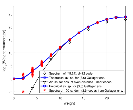
Figure 1: The theoretical and empirical spectra of $(3,6)$-regular Gallager codes of length $n=48$. The average spectrum for the Gallager ensemble and for the ensemble of even-distance linear codes are defined by (9) and (6), respectively.

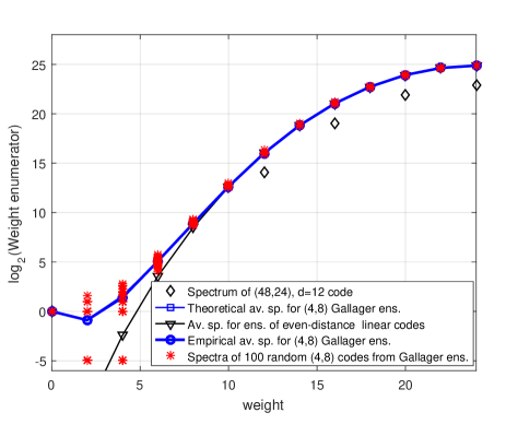
Figure 2: The theoretical and empirical spectra of $(4,8)$-regular Gallager codes of length $n=48$. The average spectrum for the Gallager ensemble and for the ensemble of even-distance linear codes are defined by (9) and (6), respectively.

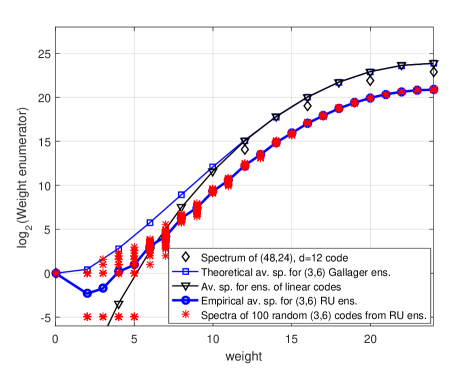
Figure 3: The theoretical spectrum of $(3,6)$-regular Gallager codes and the empirical spectra of $(3,6)$-RU LDPC codes of length $n=48$. The average spectrum for the Gallager ensemble and for the ensemble of random linear codes are defined by (9) and (5), respectively.

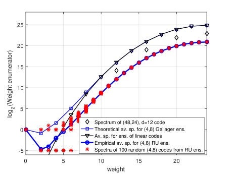
Figure 4: The theoretical spectrum of $(4,8)$-regular Gallager codes and the empirical spectra of $(4,8)$-RU LDPC codes of length $n=48$. The average spectrum for the Gallager ensemble and for the ensemble of random linear codes are defined by (9) and (5), respectively.

In Figs. 1 and 2, we present the average spectrum for the Gallager ensemble and the average spectrum for the ensemble of random linear codes with only even-weight codewords, computed using formulas from Section III-B, spectra of $100$ random codes from the Gallager ensemble, and the empirical average spectrum computed over $100$ random codes from the same ensemble. The spectrum of a quasi-perfect $[48,24]$ linear code with minimum distance $d=12$ is presented in the same figures as well. In Figs. 3 and 4, the average spectrum for the Gallager ensemble and the average spectrum for the ensemble of random linear codes are compared with the spectra of $100$ random codes from the RU ensemble and the empirical average spectrum computed over $100$ random codes from the RU ensemble. In Figs. 1–4, we use a negative value ($-5$) for the logarithm of a spectrum coefficient to indicate that the corresponding coefficient is zero.

We make the following observations regarding the Gallager codes:

• For the Gallager $(3,6)$ and $(4,8)$-regular LDPC codes their empirical average spectra perfectly match with the theoretical average spectra computed for the corresponding ensembles.

• For all codes from the Gallager ensemble the number of high-weight codewords is perfectly predicted by the theoretical average spectrum.

• The number of low-weight codewords has large variation.

We make the following remarks about the RU codes:

• Most of the RU LDPC codes are indeed irregular and have codewords of both even and odd weight.

• Typically, parity-check matrices of random codes from the RU ensemble have full rank, and these codes have lower rate than LDPC codes from the Gallager ensemble. For this reason, the empirical average spectrum of the RU ensemble lies below the theoretical average spectrum computed for the Gallager ensemble.

• The average distance properties of the RU codes are better than those of the Gallager codes.

• The variation of the number of low-weight codewords is even larger than that for the Gallager codes.

Since for all considered ensembles low-weight codewords have a much larger probability than for general linear codes, we expect to observe a higher error floor.

IV Error probability bounds on the BEC

In this section, we present a new tightened lower bound (Theorem 2) on the ML decoding error probability for linear codes and two new upper bounds (Theorem 3, Theorem 4) on the ML decoding error probability for the RU and Gallager ensembles, respectively.

IV-A Lower bounds

We start with a simple lower bound which is true for any linear code.

Theorem 1:

$$P_{e}\geq P_{e}(n,k,\varepsilon)\triangleq\sum_{i=r+1}^{n}\binom{n}{i}\varepsilon^{i}(1-\varepsilon)^{n-i}\;.$$ (10)

Remark 1:

[10, Theorem 38] gives a lower bound on the error probability of ML decoding. It differs from (10) by a multiplier which is close to $1$. This difference appears because of different definitions of the frame error event in this paper and in [10, Theorem 38].

Proof:

It readily follows from the definition of the decoding error probability and from the condition in (3) that if the number of erasures $\nu>r\geq\mbox{rank}\left(H\right)$, then the decoding error probability is equal to one. ∎

The bound (10) ignores erasure combinations of weight less than or equal to $r$. Such combinations lead to an error if they cover all nonzero entries of a codeword.

Theorem 2:

Let the code minimum distance be $d_{\min}\leq d_{0}$. Then,

$$P_{e}\geq P_{e}(n,k,\varepsilon)+\sum_{w=d_{0}}^{r}\binom{n-d_{0}}{w-d_{0}}\varepsilon^{w}(1-\varepsilon)^{n-w}\;.$$ (11)

Proof:

There is at least one nonzero codeword $\bm{c}_{0}$ of weight at most $d_{0}$ in the code. Each erasure combination of weight $w\geq d_{0}$ which covers the nonzero positions of $\bm{c}_{0}$ leads to additional decoder failures taken into account as the sum in the right-hand side (RHS) of (11). ∎

We remark that upper bounds on the minimum distance of linear codes with given $n\leq 256$ and $k$ can be found in [29]. The lower bounds (10) and (11) are compared in Fig. 5.

IV-B Upper bounds for general linear codes

Next, we consider the ensemble-average ML decoding block error probability ${\rm E}\{P_{e}\}$ over the BEC with erasure probability $\varepsilon>0$. This average decoding error probability can be interpreted as an upper bound on the achievable error probability for codes from the ensemble. In other words, there exists at least one code in the ensemble whose ML decoding error probability is upperbounded by ${\rm E}\{P_{e}\}$. To simplify notation, in the sequel we use $P_{e}$ for the ensemble-average error probability. For the ensemble of random binary $[n,n-r]$ linear codes

$$P_{e} = \sum_{\nu=r+1}^{n}\binom{n}{\nu}\varepsilon^{\nu}(1-\varepsilon)^{n-\nu}$$ (12)

$$+ \sum_{\nu=1}^{r}\binom{n}{\nu}\varepsilon^{\nu}(1-\varepsilon)^{n-\nu}P_{e|\nu}\;,$$

where $P_{e|\nu}$ denotes the conditional ensemble-average error probability given that $\nu$ erasures occurred.

By using the approach based on estimating the rank of submatrices of random matrices [30], the expression

$$P_{e|\nu}=\Pr\left(\mbox{rank}(H_{I})<\nu\right)=1-\prod_{j=0}^{\nu-1}\left(1-2^{j-r}\right)\leq 2^{\nu-r}\;,$$ (13)

where $H_{I}$ is an $r\times\nu$ submatrix of a random $r\times n$ parity-check matrix $H$, was obtained for $P_{e|\nu}$ in [31, 32, 8].

The bound obtained by combining (12) and (13) is used as a benchmark to compare the FER performance of ML decoding of LDPC codes to the FER performance of general linear codes in Figs. 5–10.

An alternative upper bound for a specific linear code with known weight enumerator has the form [31]

$$P_{e}\leq\sum_{i=d_{\rm min}}^{n}\min\left\{\binom{n}{i},\sum_{w=d_{\rm min}}^{i}A_{n,w}\binom{n-w}{i-w}\right\}\varepsilon^{i}(1-\varepsilon)^{n-i}\;.$$ (14)

In particular, this bound can be applied to random ensembles of codes with known average spectra (see Section III). We refer to this bound as the S-bound. It is presented for several ensembles in Figs. 5–10 and discussed in Section VI.

IV-C Random coding upper bounds for $(J,K)$-regular LDPC codes

In this subsection, we derive an upper bound on the ensemble-average error probability of ML decoding of the RU and Gallager ensembles of $(J,K)$-regular LDPC codes. Similarly to the approach in [8], we estimate the rank of the submatrix $H_{I}$.

A generalization of the bound in (13) to an ensemble of LDPC codes over the $q$-ary BEC is presented in [33]. Notice that the upper bound in [33] for $q$ = 2 is derived for a sparse parity-check code ensemble with column and row weights growing with the code length.

Theorem 3:

The $(J,K)$-RU ensemble-average ML decoding error probability for $[n,n-r]$ codes, $n=MK$, $r=MJ$, and $M\gg 1$, is upperbounded by

$$P_{e} \leq \sum_{\nu=r+1}^{n}\binom{n}{\nu}\varepsilon^{\nu}(1-\varepsilon)^{n-\nu}$$ (15)

$$+ \sum_{\nu=1}^{r}2^{\nu-r}\left(1+\frac{\binom{n-\nu}{K}}{\binom{n}{K}}\right)^{r}\binom{n}{\nu}\varepsilon^{\nu}(1-\varepsilon)^{n-\nu}\;.$$

Proof:

See Appendix B. ∎

The same technique leads to the following bound for the Gallager ensemble of random LDPC codes.

Theorem 4:

The $(J,K)$-Gallager ensemble-average ML decoding error probability for $[n,n-r]$ codes, $n=MK$, $r=MJ$, and $M\gg 1$, is upperbounded by

$$P_{e} \leq \sum_{\nu=1}^{r}\sum_{\mu=0}^{J(n-\nu)/K}\min\left\{1,2^{\mu+\nu-r}\right\}\min\left\{1,\binom{\mu+J-1}{J-1}\binom{M}{\mu/J}^{J}\left(\frac{n-\nu}{n}\right)^{\mu K}\right\}\binom{n}{\nu}\varepsilon^{\nu}(1-\varepsilon)^{n-\nu}$$ (16)

$$+ \sum_{\nu=r+1}^{n}\binom{n}{\nu}\varepsilon^{\nu}(1-\varepsilon)^{n-\nu}\;.$$

Proof:

See Appendix C. ∎

We refer to the bounds (15) and (16) as R-bounds, since they are based on estimating the rank of submatrices of $H$.

Computations show that while for rates close to the capacity these bounds are rather tight, for small $\varepsilon$ (or for rates significantly lower than the capacity) these bounds are weak for short codes. The reason for the bound untightness is related to the Gallager ensemble properties discussed in detail in Appendix A.

V Sliding-window near-ML decoding of QC LDPC codes

In this section, we present a new decoding algorithm for a class of QC LDPC codes. This class of codes is widely used in practice due to their extremely compact description. Moreover, under a so-called bi-diagonal structure restriction, QC LDPC codes have linear encoding complexity.

A binary QC LDPC block code can be considered as a TB parent convolutional code determined by a polynomial parity-check matrix whose entries are monomials or zeros.

A rate $R=b/c$ parent LDPC convolutional code can be determined by its polynomial parity-check matrix

$$H(D)=\left(\begin{array}[]{cccc}h_{11}(D)&h_{12}(D)&\dots&h_{1c}(D)\\ h_{21}(D)&h_{22}(D)&\dots&h_{2c}(D)\\ \vdots&\vdots&\ddots&\vdots\\ h_{(c-b)1}(D)&h_{(c-b)2}(D)&\dots&h_{(c-b)c}(D)\end{array}\right)\;,$$ (17)

where $D$ is a formal variable, $h_{ij}(D)$ is either zero or a monomial entry, that is, $h_{ij}(D)\in\{0,D^{w_{ij}}\}$ with $w_{ij}$ being a nonnegative integer, and $\mu=\max_{i,j}\{w_{ij}\}$ is the syndrome memory.

The polynomial matrix (17) determines an $[M_{0}c,M_{0}b]$ QC LDPC block code using a set of polynomials modulo $D^{M_{0}}-1$. If $M_{0}\to\infty$ we obtain an LDPC convolutional code which is considered as a parent convolutional code with respect to the QC LDPC block code for any finite $M_{0}$. By tailbiting the parent convolutional code to length $M_{0}>\mu$, we obtain the binary parity-check matrix

$$H_{\rm TB}=\begin{pmatrix}H_{0}&H_{1}&\dots&H_{\mu-1}&H_{\mu}&{\bm{0}}&\dots&\bm{0}\\ {\bm{0}}&H_{0}&H_{1}&\dots&H_{\mu-1}&H_{\mu}&\dots&\bm{0}\\ \vdots&&\ddots&\vdots&\vdots&\vdots&\ddots&\\ H_{\mu}&{\bm{0}}&\dots&\bm{0}&H_{0}&H_{1}&\dots&H_{\mu-1}\\ \vdots&\ddots&\vdots&\vdots&\vdots&\vdots&\vdots&\vdots\\ H_{1}&\dots&H_{\mu}&{\bm{0}}&\dots&\bm{0}&\dots&H_{0}\end{pmatrix}$$

of an equivalent (in the sense of column permutation) TB code (all matrices $H_{i}$ including $H_{\rm TB}$ should have a transpose operator to get the exact TB code [34]), where $H_{i}$, $i=0,1,\dotsc,\mu$, are the binary $(c-b)\times c$ matrices in the series expansion

$$H(D)=H_{0}+H_{1}D+\cdots+H_{\mu}D^{\mu}\;.$$

If every column and row of $H(D)$ contains $J$ and $K$ nonzero entries, respectively, we call $\mathcal{C}$ a $(J,K)$-regular QC LDPC code and irregular otherwise.

Notice that by zero-tail termination [34] of (17) at length $W>\mu$, we can obtain a parity-check matrix of a $[Wc,(W-\mu)b]$ ZT QC LDPC code.

Consider a BEC with erasure probability $\varepsilon>0$. Let $H$ be an $M_{0}(c-b)\times M_{0}c$ parity-check matrix of a binary $[n=M_{0}c,k=M_{0}b,d_{\min}]$ QC LDPC block code, where $d_{\min}$ is the minimum Hamming distance of the code. An ML decoder corrects any pattern of $\nu$ erasures if $\nu\leq d_{\min}-1$. If $d_{\min}\leq\nu\leq n-k$, then a unique correct decision can be obtained for some erasure patterns. The number of such correctable patterns depends on the code structure.

As explained in Section II, ML decoding over the BEC is equivalent to solving (1). Furthermore, it is well-known that solving a system of $t$ sparse linear equations requires $O(t^{2})$ operations [35],[36]. Typically, ML decoding of LDPC codes is performed in the form of hybrid decoding combining standard iterative decoding with an additional decoding step applied to the result of the BP decoding in case it fails (see, for example, [15], [16]). The computational complexity of hybrid decoding of LDPC codes over the BEC is of order $\nu^{2}$, where $\nu\approx(1-R)n$. A thorough complexity analysis of pivoting strategies for hybrid decoding of LDPC codes is presented in [15]. It was shown in [16] that for a specified class of QC LDPC codes, the complexity of hybrid decoding can be reduced to $O(\nu\sqrt{\nu})$. This technique can be efficiently applied either to the decoding of short and moderate length QC LDPC codes or to the decoding of rather long high rate QC LDPC codes. In [17], a near-linear time ML decoding algorithm based on a simplified Gaussian elimination technique for long (in the order of tens of thousands of bits) Raptor codes where $r\ll n$ (code redundancy is about $1$ percent) was studied. However, if both $r$ and $n$ are in the order of tens of thousands of bits, ML decoding of LDPC (or QC LDPC) codes over the BEC is still considered computationally intractable.

In order to overcome this limitation, low-complexity near-ML decoding algorithms were proposed in [21], [24]. They are based on guessing codeword bits when standard BP decoding fails. This type of decoding algorithms requires a number of trials of BP decoding equal to, at least, a polynomial function of the number of bit guesses. Notice that the number of bit guesses grows with the channel erasure probability. The algorithm in [24] improves the bit guessing rule compared to the one used in [21]. The suggested improvement is based on the observation that, typically, at lower channel erasure probabilities, the fraction of weight-two checks among the unsatisfied checks is significant. This allows to simplify decoding by replacing the corresponding pairs of variables by one variable. In [21] and [24], the suggested algorithms were evaluated and compared based only on their simulated BER performance.

In this paper, we follow another approach, which takes into account the similarity of decoding techniques for convolutional codes and those of QC block codes. The proposed algorithm resembles wrap-around suboptimal decoding of TB convolutional codes [25, 26]. The main idea behind this approach is that Viterbi decoding is applied to the wrapped-around trellis of a TB code with all initial state metrics equal to zero instead of running a separate Viterbi decoding from each initial state. This approach yields near-ML decoding performance with a linear number of decoding trials of Viterbi decoding. We apply this idea to QC LDPC codes.

It is shown in [37] that iterative decoding thresholds of regular LDPC convolutional codes closely approach the ML decoding thresholds of the corresponding regular LDPC block codes. However, this is not the case for block LDPC codes. In order to improve the decoding performance for block LDPC codes, we apply a sliding-window decoding algorithm which is modified for QC LDPC block codes. The suggested decoding algorithm is a hybrid decoding algorithm where BP decoding of the QC LDPC code is followed by so-called SWML decoding. The latter technique is applied “quasi-cyclically” to a relatively short sliding window, where the decoder performs ML decoding of a ZT LDPC convolutional code. The decoding complexity of the proposed algorithm (simply referred to as SWML decoding in the sequel) is polynomial (at most cubic) in the window length, but only linear in the code length. Owing to the low computational complexity, the proposed hybrid decoding algorithm can be used for decoding codes of lengths in the order of hundreds of thousands of bits, but its decoding performance is limited by the maximum degree of the monomials in the parity-check matrix of its parent LDPC convolutional code that in turn is restricted by the window size.

The SWML decoder is determined by a binary parity-check matrix

$$H_{\rm W}=\left(\begin{array}[]{ccccccc}H_{0}&\dots&H_{\mu}&{\bm{0}}&\bm{0}&\dots&{\bm{0}}\\ {\bm{0}}&H_{0}&\dots&H_{\mu}&\bm{0}&\dots&{\bm{0}}\\ \vdots&\ddots&\ddots&&\ddots&\ddots&\vdots\\ \bm{0}&\dots&\bm{0}&H_{0}&\dots&H_{\mu}&\bm{0}\\ \bm{0}&\bm{0}&\dots&{\bm{0}}&H_{0}&\dots&H_{\mu}\\ \end{array}\right)$$ (23)

of size $(W-\mu)(c-b)\times Wc$, where $W\geq 2\mu+1$ denotes the size of the decoding window in blocks. The parity-check matrix (23) determines a ZT LDPC parent convolutional code. We start decoding with BP decoding applied to the original QC LDPC block code of length $n=M_{0}c$, and then apply ML decoding to the ZT LDPC parent convolutional code determined by the parity-check matrix (23). It implies solving a system of linear equations

$${\bm{x}}_{I,\rm W}H^{\rm T}_{I,\rm W}=\bm{s}_{\rm W}\;,$$

where ${\bm{x}}_{I,\rm W}=(x_{I,{\rm W},i},x_{I,{\rm W},i+1\bmod n},\dotsc,x_{I,{\rm W},i+Wc-1\bmod n})$, $i=0,s,2s,\dotsc\bmod n$ is a subvector of ${\bm{x}}_{I}$ corresponding to the chosen window, $s$ denotes the size of the window shift, and ${\bm{s}}_{\rm W}$ and $H_{I,\rm W}$ are the corresponding subvector of ${\bm{s}}$ and submatrix of $H_{I}$, respectively. The final decision is made after $\alpha n/s$ steps, where $\alpha$ denotes the number of passes of sliding-window decoding. The formal description of the decoding procedure is given below as Algorithms 1 and 2.

Notice that the choice of $s$ affects both the performance and the complexity. By increasing $s$ we can speed up the decoding procedure at the cost of some performance loss. In the sequel, we use $s=c$ bits that corresponds to the lowest possible FER.

while there exist parity checks with only one erased symbol do

Assign to the erased symbol the modulo-$2$ sum of all nonerased symbols participating in the same parity check.

end while

Algorithm 1 BP-BEC

Input: BEC output $\bm{y}$.

Perform BP decoding of $\bm{y}$.

${\rm wstart}\leftarrow 0$;

${\rm wend}\leftarrow W-1$;

$\rm corrected\leftarrow 1$;

while $\rm corrected>0$ do

     $\rm corrected\leftarrow 0$;

     Apply ML decoding to the window $(y_{\rm wstart},\dotsc,y_{\rm{wend}})$;

     ${\rm wstart\leftarrow{\rm wstart}}+s\bmod n$;

     ${\rm wend\leftarrow\rm wend}+s\bmod n$;

     if $\rm wstart=0$ then

         corrected $\leftarrow$ number of corrected erasures after a full round;

     end if

end while

return $\bm{y}$

Algorithm 2 Wrap-around algorithm for near-ML decoding of QC LDPC codes over the BEC

Next, we present an example of selecting window positions in the parity-check matrix $H$ of the QC LDPC code. The window size in blocks is equal to $(W-\mu)\times W=(7-3)\times 7$. The two first and three last window positions in each pass are shown.

Example 1:

$$\small H=\left(\>\begin{array}[]{*{8}{c}}\cline{1-7}\cr\vrule\lx@intercol\hfil H_{0}\hfil\lx@intercol&H_{1}&H_{2}&H_{3}&\bf{0}&\bf{0}&\lx@intercol\hfil\bf{0}\hfil\lx@intercol\vrule\lx@intercol&\bf{0}\\ \vrule\lx@intercol\hfil\bf{0}\hfil\lx@intercol&H_{0}&H_{1}&H_{2}&H_{3}&\bf{0}&\lx@intercol\hfil\bf{0}\hfil\lx@intercol\vrule\lx@intercol&\bf{0}\\ \vrule\lx@intercol\hfil\bf{0}\hfil\lx@intercol&\bf{0}&H_{0}&H_{1}&H_{2}&H_{3}&\lx@intercol\hfil\bf{0}\hfil\lx@intercol\vrule\lx@intercol&\bf{0}\\ \vrule\lx@intercol\hfil\bf{0}\hfil\lx@intercol&\bf{0}&\bf{0}&H_{0}&H_{1}&H_{2}&\lx@intercol\hfil H_{3}\hfil\lx@intercol\vrule\lx@intercol&\bf{0}\\ \cline{1-7}\cr{\bf 0}&{\bf 0}&{\bf 0}&{\bf 0}&H_{0}&H_{1}&H_{2}&H_{3}\\ H_{3}&{\bf 0}&{\bf 0}&{\bf 0}&{\bf 0}&H_{0}&H_{1}&H_{2}\\ H_{2}&H_{3}&{\bf 0}&{\bf 0}&{\bf 0}&{\bf 0}&H_{0}&H_{1}\\ H_{1}&H_{2}&H_{3}&{\bf 0}&{\bf 0}&{\bf 0}&{\bf 0}&H_{0}\\ \end{array}\right)\;,$$

$$\small H=\left(\>\begin{array}[]{*{8}{c}}H_{0}&H_{1}&H_{2}&H_{3}&\bf{0}&\bf{0}&\bf{0}&\bf{0}\\ \cline{2-8}\cr\bf{0}&\vrule\lx@intercol\hfil H_{0}\hfil\lx@intercol&H_{1}&H_{2}&H_{3}&\bf{0}&\bf{0}&\lx@intercol\hfil\bf{0}\hfil\lx@intercol\vrule\lx@intercol\\ \bf{0}&\vrule\lx@intercol\hfil\bf{0}\hfil\lx@intercol&H_{0}&H_{1}&H_{2}&H_{3}&\bf{0}&\lx@intercol\hfil\bf{0}\hfil\lx@intercol\vrule\lx@intercol\\ \bf{0}&\vrule\lx@intercol\hfil\bf{0}\hfil\lx@intercol&\bf{0}&H_{0}&H_{1}&H_{2}&H_{3}&\lx@intercol\hfil\bf{0}\hfil\lx@intercol\vrule\lx@intercol\\ {\bf 0}&\vrule\lx@intercol\hfil{\bf 0}\hfil\lx@intercol&{\bf 0}&{\bf 0}&H_{0}&H_{1}&H_{2}&\lx@intercol\hfil H_{3}\hfil\lx@intercol\vrule\lx@intercol\\ \cline{2-8}\cr H_{3}&{\bf 0}&{\bf 0}&{\bf 0}&{\bf 0}&H_{0}&H_{1}&H_{2}\\ H_{2}&H_{3}&{\bf 0}&{\bf 0}&{\bf 0}&{\bf 0}&H_{0}&H_{1}\\ H_{1}&H_{2}&H_{3}&{\bf 0}&{\bf 0}&{\bf 0}&{\bf 0}&H_{0}\\ \end{array}\right)\;,$$

$$\vdots$$

$$\small H=\left(\>\begin{array}[]{*{8}{c}}\vrule\lx@intercol\hfil H_{0}\hfil\lx@intercol&H_{1}&H_{2}&\lx@intercol\hfil H_{3}\hfil\lx@intercol\vrule\lx@intercol&\bf{0}&\vrule\lx@intercol\hfil\bf{0}\hfil\lx@intercol&\bf{0}&\lx@intercol\hfil\bf{0}\hfil\lx@intercol\vrule\lx@intercol\\ \cline{1-4}\cr\cline{6-8}\cr\bf{0}&H_{0}&H_{1}&H_{2}&H_{3}&\bf{0}&\bf{0}&\bf{0}\\ \bf{0}&\bf{0}&H_{0}&H_{1}&H_{2}&H_{3}&\bf{0}&\bf{0}\\ \bf{0}&\bf{0}&\bf{0}&H_{0}&H_{1}&H_{2}&H_{3}&\bf{0}\\ \bf{0}&\bf{0}&\bf{0}&\bf{0}&H_{0}&H_{1}&H_{2}&H_{3}\\ \cline{1-4}\cr\cline{6-8}\cr\vrule\lx@intercol\hfil H_{3}\hfil\lx@intercol&{\bf 0}&{\bf 0}&\lx@intercol\hfil\bf{0}\hfil\lx@intercol\vrule\lx@intercol&\bf{0}&\vrule\lx@intercol\hfil H_{0}\hfil\lx@intercol&H_{1}&\lx@intercol\hfil H_{2}\hfil\lx@intercol\vrule\lx@intercol\\ \vrule\lx@intercol\hfil H_{2}\hfil\lx@intercol&H_{3}&{\bf 0}&\lx@intercol\hfil\bf{0}\hfil\lx@intercol\vrule\lx@intercol&{\bf{0}}&\vrule\lx@intercol\hfil\bf{0}\hfil\lx@intercol&H_{0}&\lx@intercol\hfil H_{1}\hfil\lx@intercol\vrule\lx@intercol\\ \vrule\lx@intercol\hfil H_{1}\hfil\lx@intercol&H_{2}&H_{3}&\lx@intercol\hfil\bf{0}\hfil\lx@intercol\vrule\lx@intercol&\lx@intercol\hfil\bf{0}\hfil\lx@intercol\vrule\lx@intercol&{\bf{0}}&{\bf{0}}&\lx@intercol\hfil H_{0}\hfil\lx@intercol\vrule\lx@intercol\\ \end{array}\right)\;,$$

$$\small H=\left(\>\begin{array}[]{*{8}{c}}\vrule\lx@intercol\hfil H_{0}\hfil\lx@intercol&H_{1}&H_{2}&{H_{3}}&\lx@intercol\hfil\bf{0}\hfil\lx@intercol\vrule\lx@intercol&{\bf{0}}&\vrule\lx@intercol\hfil\bf{0}\hfil\lx@intercol&\lx@intercol\hfil\bf{0}\hfil\lx@intercol\vrule\lx@intercol\\ \vrule\lx@intercol\hfil\bf{0}\hfil\lx@intercol&H_{0}&H_{1}&H_{2}&\lx@intercol\hfil H_{3}\hfil\lx@intercol\vrule\lx@intercol&\bf{0}&\vrule\lx@intercol\hfil\bf{0}\hfil\lx@intercol&\lx@intercol\hfil\bf{0}\hfil\lx@intercol\vrule\lx@intercol\\ \cline{1-5}\cr\cline{7-8}\cr\bf{0}&\bf{0}&H_{0}&H_{1}&H_{2}&H_{3}&\bf{0}&\bf{0}\\ \bf{0}&\bf{0}&\bf{0}&H_{0}&H_{1}&H_{2}&H_{3}&\bf{0}\\ \bf{0}&\bf{0}&\bf{0}&\bf{0}&H_{0}&H_{1}&H_{2}&H_{3}\\ H_{3}&{\bf 0}&{\bf 0}&\bf{0}&\bf{0}&H_{0}&H_{1}&H_{2}\\ \cline{1-5}\cr\cline{7-8}\cr\vrule\lx@intercol\hfil H_{2}\hfil\lx@intercol&H_{3}&{\bf 0}&{\bf{0}}&{\bf{0}}&\vrule\lx@intercol\hfil\bf{0}\hfil\lx@intercol&\vrule\lx@intercol\hfil H_{0}\hfil\lx@intercol&\lx@intercol\hfil H_{1}\hfil\lx@intercol\vrule\lx@intercol\\ \vrule\lx@intercol\hfil H_{1}\hfil\lx@intercol&H_{2}&H_{3}&{\bf{0}}&\lx@intercol\hfil\bf{0}\hfil\lx@intercol\vrule\lx@intercol&{\bf{0}}&\vrule\lx@intercol\hfil\bf{0}\hfil\lx@intercol&\lx@intercol\hfil H_{0}\hfil\lx@intercol\vrule\lx@intercol\\ \end{array}\right)\;,$$

$$\small H=\left(\>\begin{array}[]{*{8}{c}}\vrule\lx@intercol\hfil H_{0}\hfil\lx@intercol&H_{1}&H_{2}&{H_{3}}&{\bf{0}}&\lx@intercol\hfil\bf{0}\hfil\lx@intercol\vrule\lx@intercol&\lx@intercol\hfil\bf{0}\hfil\lx@intercol\vrule\lx@intercol&\lx@intercol\hfil\bf{0}\hfil\lx@intercol\vrule\lx@intercol\\ \vrule\lx@intercol\hfil\bf{0}\hfil\lx@intercol&H_{0}&H_{1}&H_{2}&{H_{3}}&\lx@intercol\hfil\bf{0}\hfil\lx@intercol\vrule\lx@intercol&\lx@intercol\hfil\bf{0}\hfil\lx@intercol\vrule\lx@intercol&\lx@intercol\hfil\bf{0}\hfil\lx@intercol\vrule\lx@intercol\\ \vrule\lx@intercol\hfil\bf{0}\hfil\lx@intercol&\bf{0}&H_{0}&H_{1}&H_{2}&\lx@intercol\hfil H_{3}\hfil\lx@intercol\vrule\lx@intercol&\lx@intercol\hfil\bf{0}\hfil\lx@intercol\vrule\lx@intercol&\lx@intercol\hfil\bf{0}\hfil\lx@intercol\vrule\lx@intercol\\ \cline{1-6}\cr\cline{8-8}\cr\bf{0}&\bf{0}&\bf{0}&H_{0}&H_{1}&H_{2}&H_{3}&\bf{0}\\ \bf{0}&\bf{0}&\bf{0}&\bf{0}&H_{0}&H_{1}&H_{2}&H_{3}\\ H_{3}&{\bf 0}&{\bf 0}&\bf{0}&\bf{0}&H_{0}&H_{1}&H_{2}\\ {H_{2}}&H_{3}&{\bf 0}&{\bf{0}}&{\bf{0}}&{\bf{0}}&{H_{0}}&{H_{1}}\\ \cline{1-6}\cr\cline{8-8}\cr\vrule\lx@intercol\hfil H_{1}\hfil\lx@intercol&H_{2}&H_{3}&{\bf{0}}&{\bf{0}}&\lx@intercol\hfil\bf{0}\hfil\lx@intercol\vrule\lx@intercol&\lx@intercol\hfil\bf{0}\hfil\lx@intercol\vrule\lx@intercol&\lx@intercol\hfil H_{0}\hfil\lx@intercol\vrule\lx@intercol\\ \end{array}\right)\;.$$

VI Numerical results and simulations

VI-A Short codes

In Fig. 5, we compare upper and lower bounds on the error probability of ML decoding of short codes on the BEC. First, notice that the lower bounds in Theorems 1 and 2 (sphere packing and the tightened sphere packing bound) almost coincide with each other near the channel capacity. However, the new bound is significantly tighter than the known one in the low erasure probability region. For further comparisons we use the new bound whenever information on the code minimum distance is available. The upper bounds in Theorems 3 and 4 are also presented in Fig. 5. These two bounds are indistinguishable at high symbol erasure probabilities but the difference between them is visible in the low $\varepsilon$ region where all bounds are rather weak. Notice that for high $\varepsilon$ random coding bounds for LDPC codes are close to those of random linear codes. For $(J,K)$-regular LDPC codes with $J=4$, both S and R-bounds are almost as good as the random bound for general linear codes of the same length and dimension in a wide range of $\varepsilon$ values. In Fig. 5, as well as in subsequent figures, S-bounds (14) are computed based on the ensemble average spectra of the corresponding $(J,K)$-regular Gallager code ensembles by using the recurrent procedure described in Section III.

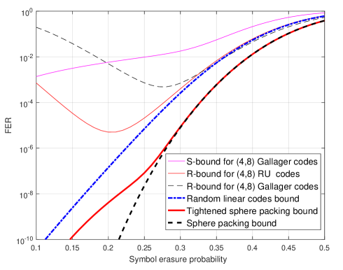
Figure 5: Bounds for binary $(4,8)$-regular LDPC codes of length $n=96$ and rate $R=1/2$. The S-bound is defined by (14), and R-bounds for RU and Gallager codes are defined by (15) and (16), respectively. The random coding bound is computed by (12)–(13), while the sphere packing bound and the tightened sphere packing bound are computed according to (10) and (11), respectively.

In Fig. 6, we compare upper bounds on the ML decoding FER performance for the Gallager ensemble of $(J,K)$-regular LDPC codes with different pairs $(J,K)$ to the upper bounds for general linear codes of different code rates. Interestingly, the convergence rate of the bounds for LDPC codes to the bounds for linear codes depends on the code rate. For rate $R=1/3$, even for rather sparse codes with column weight $J=4$, their FER performance under ML decoding is very close to the FER performance of general linear codes.

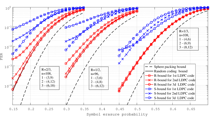
Figure 6: Error probability bounds for the binary $(J,K)$-regular Gallager LDPC codes of length $n\approx 100$. The S and R-bounds are defined by (14) and (16), respectively. Random coding bound for linear codes is computed by (12)–(13). The lower bound is (11).

Next, we present simulation results for two ensembles of LDPC codes. In Fig. 7, we compare the best code among $10$ randomly selected $(3,6)$-regular LDPC codes and the best code among $10$ randomly selected $(4,8)$-regular LDPC codes of the two ensembles. As predicted by bounds, the ML decoding performance of the $(4,8)$-regular codes is much better than that of the $(3,6)$-regular codes in both ensembles. Notice that codes from the Gallager ensemble are weaker than the RU codes with the same parameters. This can be explained by the rate bias, the code rate for the RU codes is typically equal to $R=1/2$, whereas for the Gallager codes the rate is $R\geq 52/96=0.5417$. A second reason to the difference in the FER performance is the approximation discussed in Appendix A. The performance of the RU codes perfectly matches the R-bound. Moreover, the best $(4,8)$-RU code shows even better FER performance than the average FER performance of general linear codes in the high erasure probability region.

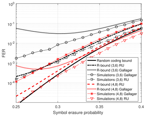
Figure 7: Simulation results for $(3,6)$-regular and $(4,8)$-regular codes of length $n=96$ from the Gallager and RU ensembles. The S-bound is defined by (14), and R-bounds for RU and Gallager codes are defined by (15) and (16), respectively. The random coding bound for linear codes is computed by (12)–(13).

VI-B Codes of moderate length

The FER performance for relatively long codes of length $n=1008$ is shown in Fig. 8. Notice that the difference between the lower and upper bounds for general linear codes, which was noticeable for short codes becomes very small for $n=1008$. Since the lower bound (10) is simply the probability of more than $r$ erasures, the fact that the upper and the lower bounds almost coincide leads us to the conclusion that even for rather low channel erasure probabilities $\varepsilon$, achieving ML decoding performance requires correcting almost all combinations of erasures of weight close to the code redundancy $r$. Notice that according to the S-bounds in Fig. 8, error floors are expected in the low erasure probability region. The error-floor level strongly depends on $J$ and $K$, and rapidly decreases with increasing $J$.

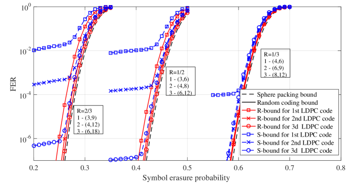
Figure 8: Error probability bounds for the binary $(J,K)$-regular Gallager LDPC codes of length $n=1008$. S and R-bounds are defined by (14) and (16), respectively. The random coding bound for linear codes is computed by (12)–(13). The lower bound is (11).

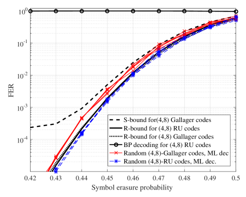
Figure 9: Error probability bounds and simulation results for $(4,8)$-regular LDPC codes of length $n=1008$. The S-bound is defined by (14), and R-bounds for the RU and Gallager codes are defined by (15) and (16), respectively.

In Fig. 9, we show simulation results for $5$ randomly selected $(4,8)$-regular codes of length $n=1008$, respectively, from the Gallager and RU ensembles. Notice that the simulated performance for $5$ randomly selected $(3,6)$-regular codes of the same length demonstrates similar behaviour and for this reason is not presented in the plot. In the same plots the rank and spectral bounds for the corresponding ensembles are shown. We observe that for rates close to the capacity, the rank and spectral bounds demonstrate approximately the same behavior. For low channel erasure probabilities the spectral bound predicts error floors. As expected, the spectral bound is weak for rates far below the channel capacity. Since all $10$ codes ($5$ for the Gallager ensemble and $5$ for the RU ensemble) show identical FER performance, we present only one of the BP decoding FER curves in the figure.

VI-C Sliding-window near-ML decoding of QC LDPC codes

We compare the FER performance of BP and SWML decoding for three QC LDPC codes of length $M_{0}c=4800$ to the S and R upper bounds on the ML decoding performance. The parameters of the codes, including the minimum distance $d_{\min}$ and the stopping distance $d_{\rm stop}$ of the QC LDPC code of length $Wc$, where $W$ is the window size in blocks, and the SWML decoder parameters are summarized in Table I. The irregular rate $R=12/24$ QC LDPC code is determined by the monomial parity-check matrix of its parent convolutional code optimized by the technique described in [38]. This matrix has the form

$$H(D)=\left(\begin{array}[]{cc}H_{\rm{bd}}(D)&H_{\rm{a}}(D)\end{array}\right)\;,$$ (24)

where $H_{\rm{bd}}$ is a bidiagonal matrix of size $12\times 11$ with ones on the diagonals and zeros elsewhere, and $H_{\rm a}$ is a $12\times 13$ matrix whose degree matrix is

$$\small\begin{pmatrix}\begin{array}[]{rrrrrrrrrrrrr}0&-1&-1&-1&0&-1&0&-1&-1&-1&-1&0&0\\ 21&-1&-1&-1&-1&0&-1&-1&-1&0&-1&-1&3\\ -1&-1&-1&0&2&-1&-1&-1&-1&-1&0&5&-1\\ -1&-1&0&-1&-1&-1&-1&-1&0&10&-1&7&-1\\ -1&-1&-1&14&-1&-1&-1&0&-1&-1&10&-1&15\\ -1&0&-1&-1&-1&20&-1&-1&7&-1&-1&11&3\\ -1&-1&6&-1&4&-1&-1&-1&-1&9&-1&-1&0\\ -1&18&-1&-1&-1&-1&13&-1&-1&-1&7&19&14\\ -1&-1&-1&21&-1&3&-1&-1&-1&11&-1&17&13\\ -1&21&-1&-1&-1&-1&-1&19&-1&2&-1&12&14\\ 0&-1&-1&-1&-1&-1&-1&-1&18&-1&11&2&1\\ -1&-1&12&-1&-1&-1&5&15&-1&-1&17&9&-1\end{array}\end{pmatrix}\,.$$ (25)

The polynomial parity-check matrix $H(D)$ is obtained from this degree matrix by replacing each negative entry with a zero, and replacing each nonnegative entry $e$ with $D^{e}$.

A regular rate $R=3/6$ QC LDPC code determined by the parity-check matrix of [39, Table IV] and a regular rate $R=8/16$ double-Hamming (DH) based QC LDPC code [40] determined by the degree matrix

$$\small\begin{pmatrix}\begin{array}[]{rrrrrrrrrrrrrrrrrr}11&-1&4&-1&-1&-1&-1&5&6&5&-1&-1&15&-1&3&11\\ 13&-1&-1&11&-1&-1&1&-1&13&2&-1&2&-1&13&-1&7\\ 3&-1&-1&-1&5&-1&10&9&-1&3&8&-1&-1&10&8&-1\\ 12&-1&-1&-1&-1&1&8&15&9&-1&8&4&3&-1&-1&-1\\ -1&13&-1&1&10&12&2&-1&-1&-1&-1&0&-1&6&6&-1\\ -1&11&6&-1&2&6&-1&14&-1&-1&14&-1&0&-1&2&-1\\ -1&13&3&5&-1&5&-1&-1&10&-1&-1&-1&10&12&-1&7\\ -1&3&4&10&4&-1&-1&-1&-1&3&14&11&-1&-1&-1&4\end{array}\end{pmatrix}$$

were simulated as well. The minimum and stopping distances of the codes (of length $Wc$) are computed by using the algorithm in [41], [42]. Simulation results and bounds are presented in Fig. 10.

The SWML decoding FER performance of the DH code is the best among the SWML decoding FER performances of the simulated codes and it is close to the theoretical bounds, despite its very low decoding complexity. In contrast, the FER performance of BP decoding of this code is extremely poor. This is not surprising, since on one hand, the DH code has better distance properties among the three codes, and on the other hand, its parity-check matrix is rather dense. This improves its ML decoding performance compared to the other codes and also makes it less suitable for iterative decoding. For the $(3,6)$-regular QC LDPC code, as well as for the irregular QC LDPC code, BP decoding performs much better than for the DH code, but the FER performance of SWML decoding of these codes is worse than that of the DH code. Notice that the considered irregular code has average column weight of $3.125$, which makes the comparison with the R and S-bounds for $(3,6)$ and $(4,8)$-regular codes fair. The gap between the FER performance of BP and SWML decoding of these two codes is not large. The SWML decoding performance of the $(3,6)$ regular code is worse than that of BP decoding of the irregular code despite that the minimum distance of the $(3,6)$-regular code is larger. The SWML decoding performance of the $(3,6)$-regular code mimics the behavior of the S-bound.

In Fig. 11, we compare the FER performance of BP and ML decoding for the irregular QC LDPC code of length $4800$ with the FER performance of SWML decoding with different window sizes for the same code. It is easy to see that the FER performance of SWML decoding is approaching the FER performance of ML decoding with increasing window size. The ML decoding curve is obtained by running an inactivation decoder [43].

In Figs. 12 and 13, we compare the simulated FER and BER performance of SWML decoding of three QC LDPC codes of length of a few tens of thousands of bits $(M_{0}=4000-10000)$ with the BP and ML decoding thresholds computed by the density evolution analysis [4]. Codes of rate $3/6$ and $8/16$ were obtained by increasing $M_{0}$ for the code in [39, Table IV] and the DH code, respectively. The irregular rate-$12/24$ code is determined by the parity-check matrix (24) with $H_{\rm{a}}(D)$ given by

$$\small\begin{pmatrix}\begin{array}[]{rrrrrrrrrrrrr}0&-1&-1&0&-1&-1&0&-1&-1&-1&0&0&0\\ -1&-1&-1&-1&-1&-1&-1&0&-1&0&-1&5&21\\ -1&0&-1&-1&0&-1&-1&-1&0&-1&-1&29&41\\ -1&-1&0&-1&-1&-1&-1&81&-1&-1&0&50&54\\ 55&72&-1&-1&-1&0&-1&-1&-1&-1&-1&85&5\\ -1&-1&-1&46&-1&-1&-1&-1&71&29&-1&23&24\\ -1&-1&89&-1&-1&50&-1&-1&-1&-1&-1&93&78\\ -1&-1&-1&-1&36&-1&-1&-1&-1&50&32&8&90\\ -1&-1&-1&-1&-1&-1&56&-1&26&-1&-1&9&51\\ -1&94&-1&69&-1&89&-1&-1&-1&-1&-1&84&98\\ 0&-1&-1&-1&-1&-1&-1&29&-1&-1&-1&85&8\\ -1&-1&41&-1&92&-1&13&-1&-1&-1&-1&39&83\end{array}\end{pmatrix}.$$

Parameters of the codes together with the parameters of the SWML decoder are presented in Table II. It follows from the presented curves that the SWML decoder significantly outperforms the BP decoder in the near-capacity region. Interestingly enough, unlike for regular codes, the BP decoding threshold for irregular codes computed by density evolution is much lower than the simulated achievable performance. However, due to memory restrictions, the SWML decoder does not achieve ML decoding performance of ensemble-average regular LDPC codes of the same length. Moreover, the decoding thresholds are obtained by the density evolution approach which, as well as the bounds presented in Section IV, do not take into account restrictions imposed by the quasi-cyclic structure of the codes. This fact increases the gap between the thresholds and the simulated performance.

In Fig. 14, we compare the simulated FER and BER performance of the irregular $R=12/24$ QC LDPC code of length $4800$ determined by the parity-check matrix (24) with $H_{\rm a}(D)$ given by (25) and lifting degree $M_{0}=200$ under SWML decoding with a window size of $W=51$ blocks and the BER performance of random LDPC codes of length $10^{4}$ decoded by the two bit guessing based decoding algorithms ($A$ and $C$) in [21]. Although the window size of the SWML decoder is much smaller than the code length and the code is two times shorter than the irregular codes in [21], the difference in performance is noticeable.

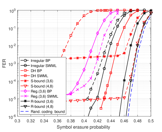
Figure 10: Error probability bounds and the simulated FER performance of SWML decoding of QC LDPC codes of length $n=4800$. S and R-bounds are defined by (14) and (15), respectively. The average FER performance of ML decoding for random linear codes is computed by (12)–(13).

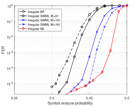
Figure 11: The simulated FER performance of BP, ML, and SWML decoding with different window sizes for an irregular $R=12/24$ QC LDPC code of length $n=4800$.

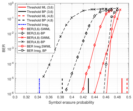
Figure 12: Comparison of the simulated BER performance of SWML decoding of irregular QC LDPC codes of length $n=60000-96000$ with BP and ML decoding thresholds.

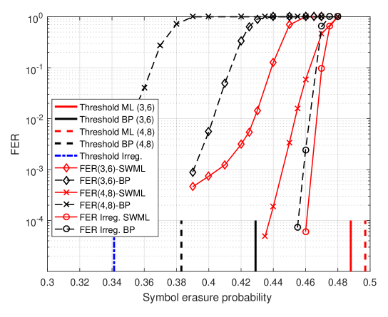
Figure 13: Comparison of the simulated FER performance of SWML decoding of irregular QC LDPC codes of length $n=60000-96000$ with BP and ML decoding thresholds.

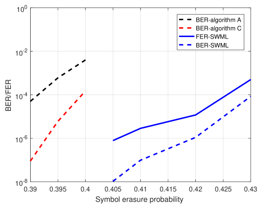
Figure 14: Comparison of the simulated FER and BER performance of SWML decoding of the irregular QC LDPC code of length $n=4800$ with the simulated BER performance of contraction-based decoding of random codes of length $10^{4}$.

TABLE I: Example parameters of SWML decoders for codes of length $n=4800$.

Code and decoder	Codes
parameters	Irregular	DH	$(3,6)$-regular
Base matrix size $b\times c$	$12\times 24$	$8\times 16$	$3\times 6$
Syndrome memory $\mu$	$21$	$15$	85
Decoding window size $W$	$51$	$81$	$171$
Window shift	$24$	$16$	$6$
Overall TB length in bits $M_{0}\times c$	$200\times 24$	$300\times 16$	$800\times 6$
Maximum number of passes	$15$	$15$	15
Minimum distance $d_{\min}$	$23$	$>24$	24
Distance spectrum	$51,306,\dots$		$2565,0,0,\dots$
Stopping distance $d_{{\rm stop}}$	$19$	$>24$	24
Stopping set spectrum	$51,0,51,0,$		$2565,0,0,\dots$
	$255,459,\dots$

TABLE II: Example parameters of SWML decoders for codes of length $n=60000-96000$.

Code and decoder	Codes
parameters	Irregular	DH	$(3,6)$-regular
Base matrix size $b\times c$	$12\times 24$	$8\times 16$	$3\times 6$
Syndrome memory $\mu$	$98$	$15$	85
Decoding window size $W$	$300$	$100$	$200$
Window shift	$24$	$16$	$6$
Overall TB length in bits $M_{0}\times c$	$4000\times 24$	$6000\times 16$	$10000\times 6$
Maximum number of passes	$15$	$15$	15

VII Thresholds

In order to obtain an asymptotic upper bound on the error probability for $(J,K)$-regular LDPC codes, we use the following inequality:

$$\frac{\binom{n-\nu}{K}}{\binom{n}{K}}\leq\left(\frac{n-\nu}{n}\right)^{K}\;.$$ (26)

For the RU ensemble, it follows from (15) that

$$P_{e} \leq \sum_{\nu=1}^{n}\min\left\{1,B_{\nu}\right\}\binom{n}{\nu}\varepsilon^{\nu}(1-\varepsilon)^{n-\nu}$$

$$\leq {n\cdot\exp\left\{-\min_{\nu}\left\{\max\left\{T_{1},T_{1}-\log B_{\nu}\right\}\right\}\right\}}\;,$$

where

$$B_{\nu} = 2^{\nu-r}\left(1+\frac{\binom{n-\nu}{K}}{\binom{n}{K}}\right)^{r}\;,$$

$$T_{1} = -\log\binom{n}{\nu}-\nu\log\varepsilon-(n-\nu)\log(1-\varepsilon)\;.$$

Denote by $\alpha=\nu/n$ the normalized number of erasures. The asymptotic error probability exponent can be written as

$$E(\varepsilon) = \lim_{n\to\infty}\left\{-\frac{\log P_{e}}{n}\right\}$$ (27)

$$\geq \min_{\alpha\in[0,1]}\left\{\max\left\{F_{1}(\alpha,\varepsilon)\;,F_{2}(\alpha,\varepsilon)\right\}\right\},$$

where

$$F_{1}(\alpha,\varepsilon) = -h(\alpha)-\alpha\log\varepsilon-(1-\alpha)\log(1-\varepsilon)\;,$$ (28)

$$F_{2}(\alpha,\varepsilon) = F_{1}(\alpha,\varepsilon)-F_{3}(\alpha)\;,$$ (29)

$$F_{3}(\alpha) = \left(\alpha-\frac{J}{K}\right)\log 2+\frac{J}{K}\left[\log\left(1+(1-\alpha)^{K}\right)\right]\;,$$ (30)

$$h(\alpha) = -\alpha\log\alpha-(1-\alpha)\log(1-\alpha)\;.$$ (31)

In (27)–(31) all logarithms are to the base of $e$. The asymptotic decoding threshold is defined as the maximum $\varepsilon$ providing $E(\varepsilon)>0$, or as the minimum $\varepsilon$ providing $E(\varepsilon)=0$. It is easy to see that $F_{1}(\alpha,\varepsilon)$ is always positive except at the point $\alpha=\varepsilon$ where $F_{1}(\alpha,\varepsilon)=0$, $F_{2}(\alpha,\varepsilon)>0$ for $\alpha<\varepsilon$, and $F_{2}(\alpha,\varepsilon)=0$ at $\alpha=\varepsilon$ if $F_{3}(\alpha)=F_{3}(\varepsilon)=0$. In other words, a lower bound on the ML decoding threshold can be found as the unique solution of the equation

$$\varepsilon=\frac{J}{K}\left[1-\frac{\log\left(1+(1-\varepsilon)^{K}\right)}{\log 2}\right]\;.$$ (32)

Notice that increasing $K$ leads to the simple expression

$$\varepsilon\xrightarrow[K\to\infty]{}\frac{J}{K}=1-R$$

for the threshold, which corresponds to the capacity of the BEC. Numerical values for the lower bound from (32) on the ML decoding threshold for different code rates and different column weights are shown in Table III.

TABLE III: Lower bounds from (32) on the ML decoding threshold for binary $(J,K)$-regular LDPC codes on the BEC. Exact values for the threshold computed from [44, Lem. 4] are given in bold in the parentheses. Lower and upper bounds on the ML decoding threshold from [12, Table I] are reported in italics.

$R$	$J$
	$3$	$4$	$5$	$6$	$8$	$9$
$1/4$	$0.74546793$			$0.74998348$		$0.74999993$
	$\bf(0.74600970)$	—	—	$\bf(0.74998850)$	—	$\bf(0.74999995)$
	$\it(0.744-0.7469)$
$1/3$		$0.66531587$		$0.66661773$	$0.66666485$
	—	$\bf(0.66565559)$	—	$\bf(0.66663252)$	$\bf(0.66666541)$	—
		$\it(0.665-0.6657)$
$1/2$	$0.48696550$	$0.49705261$	$0.49928578$	$0.49982316$	$0.49998898$	$0.49999724$
	$\bf(0.48815088)$	$\bf(0.49774086)$	$\bf(0.49948579)$	$\bf(0.49987571)$	$\bf(0.49999235)$	$\bf(0.49999809)$
	$\it(0.483-0.4913)$
$2/3$	$0.31827745$	$0.32937002$	$0.33220831$	$0.33300515$	$0.33330473$	$0.33332486$
	$\bf(0.31965317)$	$\bf(0.33025003)$	$\bf(0.33251324)$	$\bf(0.33310092)$	$\bf(0.33331344)$	$\bf(0.33332745)$
$3/4$	$0.23601407$	$0.24609298$	$0.24882167$	$0.24963402$	$0.24996371$	$0.24998853$
	$\bf(0.23732490)$	$\bf(0.24694480)$	$\bf(0.24913655)$	$\bf(0.24973987)$	$\bf(0.24997473)$	$\bf(0.24999203)$

Unlike in [12, Eq. (37), Table 1] and [13] the new lower bounds on the ML decoding thresholds presented in Table III are derived from the new upper bound on the average block error probability for the RU code ensemble. The thresholds in [12, Eq. (37), Table 1] and [13] were obtained from the bounds on the bit error probability of the average code in the ensemble. This explains the fact that the lower bounds in Table III marked by asterisk differ from the best of the lower bounds (shown in parentheses) in [13] and [12, Eq. (37), Table 1].

VIII Conclusion

Both a finite-length and an asymptotic analysis of ML decoding performance of LDPC codes on the BEC have been presented. The obtained bounds are very useful, since unlike other channel models, for the BEC, ML decoding can be implemented for rather long codes. Moreover, an efficient sliding-window decoding algorithm which provides near-ML decoding of very long codes is developed. Comparisons of the presented bounds with empirical estimates of the average error probability over sets of randomly constructed codes have shown that the new bounds are rather tight at rates close to the channel capacity even for short codes. For code length $n>1000$, the bounds are rather tight for a wide range of parameters. The new bounds lead to a simple analytical lower bound on the ML decoding threshold on the BEC for regular LDPC codes.

Appendix A

There is a weakness in the proof of Theorem 2.4 in [3] by Gallager, analogous to the one in the derivations (7)–(9) above. Formula (2.17) in [3] and (9) in this paper state that the average number of weight-$w$ binary sequences which simultaneously satisfy all parity checks in $J$ strips is

$${\rm E}\{A_{n,w}\}=\binom{n}{w}\left[\frac{N_{n,w}}{\binom{n}{w}}\right]^{J}\,,$$ (33)

where $N_{n,w}$ is the number of weight-$w$ sequences satisfying the parity checks of the first strip $H_{1}$. This formula relies on the assumption that parity checks of strips are independent. It is known that this assumption is incorrect because the strips of the parity-check matrix are always linearly dependent (the sum of the parity checks of any two strips is the all-zero sequence) and, as a consequence, the actual rate of the corresponding $(J,K)$-regular codes is higher than $1-J/K$. The fact that we intensively use the strip-independence hypothesis in our derivations motivated us to study deeper the influence of the strip independence assumption both on the conclusions in [3] and on the derivations done in this paper.

In order to verify how this assumption influences the precision of estimates, consider the following simple example.

Example 2:

Consider a $(3,3)$-regular code with $M=2$. The first strip is

$$\begin{pmatrix}1&1&1&0&0&0\\ 0&0&0&1&1&1\end{pmatrix}\;.$$

The other two strips are obtained by random permutations of the columns of this strip. In total there exist $(6!)^{2}$ LDPC codes, but most of the codes are equivalent. By taking into account that the first row in each strip determines the second row, we obtain that the choice of each code is determined by the choice of the third and fifth rows of the parity-check matrix. Thus, there are at most $\binom{6}{3}^{2}=400$ equiprobable classes of equivalent codes. We compute the average spectra over codes with a certain code dimension and the average spectrum over all codes. The obtained results are presented in Table IV.

TABLE IV: Spectra of $(3,3)$-regular LDPC codes of length $6$.

Dimension	Number of codes	Average spectrum
$2$	$288$	$\begin{pmatrix}1&0&\frac{1}{2}&0&\frac{5}{2}&0&0\end{pmatrix}$
$3$	$108$	$\begin{pmatrix}1&0&2&0&5&0&0\end{pmatrix}$
$4$	$4$	$\begin{pmatrix}1&0&6&0&9&0&0\end{pmatrix}$
Average parameters over the ensemble
$2.29$	—	$\begin{pmatrix}1&0&\frac{24}{25}&0&\frac{81}{25}&0&0\end{pmatrix}$

Notice that the lower bound on the code rate $R\geq 1-J/K=0$, but since there exist at least two rows that are linearly dependent on other rows, a tightened lower bound on the code rate is $R\geq 1-4/6=1/3$. Let us compare these empirical estimates with the Gallager bound. The generating function for the first strip is

$$g(s)=1+N_{6,2}s^{2}+N_{6,4}s^{4}=1+6s^{2}+9s^{4}\;.$$

According to (33)

$${\rm E}\{A_{6,2}\} = \binom{6}{2}\left(\frac{6}{\binom{6}{2}}\right)^{3}=\frac{24}{25}\;,$$

$${\rm E}\{A_{6,4}\} = \binom{6}{4}\left(\frac{9}{\binom{6}{4}}\right)^{3}=\frac{81}{25}\;,$$

which matches with the empirical average over all codes presented in Table IV.

These computations lead us to the following conclusions:

• In the ensemble of $(J,K)$-regular LDPC codes there are codes of different dimensions. The average spectra depend on the dimension of the code and differ from the average spectrum over all codes of the ensemble.

• The average over all codes may coincide with the Gallager estimate, but does not correspond to any particular linear code. Moreover, the estimated number of codewords (sum of all spectrum components) is not necessarily equal to a power of $2$.

Notice that if $M$ is large enough, then the influence of strip dependence on the precision of the obtained spectrum estimate is negligible. However, if $\nu\ll M$, that is, in the low $\varepsilon$ region, the assumption of strip independence should be used with caution.

Appendix B

Proof of Theorem 3

Assume that the number of erasures is $\nu>0$. The error probability of ML decoding over the BEC is estimated as the probability that $\nu$ columns of the random parity-check matrix $H$ from the RU ensemble corresponding to the erased positions are linearly dependent, $\nu\leq r$.

Let $H_{I}$ be the submatrix consisting of the columns determined by the set $I$ of the erased positions, $|I|=\nu$. We can write

$$\Pr\left(\mbox{rank}(H_{I})<\nu\right|\nu)\leq\sum_{\bm{x}_{I}\neq\bm{0}}\Pr\left(\bm{x}_{I}H_{I}^{\rm T}=\bm{0}\right|\nu)\;.$$ (34)

Consider a random vector $\bm{s}=\bm{x}_{I}H_{I}^{\rm T}$. Denote by $\bm{s}_{i}^{j}$ the subvector $(s_{i},\dotsc,s_{j})$ of the vector $\bm{s}$. The probability of $\bm{s}$ being the all-zero vector is

$$p(\bm{s}=\bm{0}|\nu)=p(s_{1}=0|\nu)\prod_{i=2}^{r}p(s_{i}=0|\bm{s}_{1}^{i-1}=\bm{0},\nu)\;.$$ (35)

Next, we prove that $p(s_{1}=0|\nu)\geq p(s_{i}=0|\bm{s}_{1}^{i-1}=\bm{0},\nu)$, $i=2,3\dotsc,r$. We denote by $\nu_{i}$ the number of erasures in nonzero positions of the $i$-th parity check. For the choice of a random vector $\bm{x}$ and a random parity-check matrix from the RU ensemble the probability of a zero syndrom component $s_{i}$ is

$$p(s_{i}=0|\nu_{i})=\left\{\begin{array}[]{ll}1,&\nu_{i}=0\\ \frac{1}{2},&\nu_{i}>0\end{array}\right.\;.$$ (36)

First, we observe that for all $i$

$$p(s_{i}=0|\nu) = p(s_{i}=0|\nu_{i}=0,\nu)p(\nu_{i}=0|\nu)+p(s_{i}=0|\nu_{i}>0,\nu)p(\nu_{i}>0|\nu)$$ (37)

$$= {1\cdot p(\nu_{i}=0|\nu)+\frac{1}{2}\cdot(1-p(\nu_{i}=0|\nu))}$$

$$= \frac{1+p(\nu_{i}=0|\nu)}{2}\;.$$

For all $i\neq j$, let $K^{\prime}$ denote the number of row positions in which the corresponding elements either in row $j$ or in row $i$ of $H$ are nonzero. Since $K^{\prime}\geq K$ the following inequality holds:

$$p(\nu_{j}=0|\nu_{i}=0,\nu) = \frac{\binom{n-K^{\prime}}{\nu}}{\binom{n}{\nu}}$$ (38)

$$\leq \frac{\binom{n-K}{\nu}}{\binom{n}{\nu}}$$

$$= p(\nu_{j}=0|\nu)\;.$$

For the second parity check, by using arguments similar to those in (37), we obtain

$$p(s_{2}=0|s_{1}=0,\nu)=\frac{1}{2}\left(1+p(\nu_{2}=0|s_{1}=0,\nu)\right)\;.$$ (39)

The conditional probability in the RHS can be estimated as

$$p(\nu_{2}=0|s_{1}=0,\nu) = \sum_{\nu_{1}=0}^{\min\{K,\nu\}}p(\nu_{2}=0|s_{1}=0,\nu_{1},\nu)p(\nu_{1}|s_{1}=0,\nu)$$ (40)

$$\stackrel{{\scriptstyle(a)}}{{=}} \sum_{\nu_{1}=0}^{K}p(\nu_{2}=0|\nu_{1},\nu)\frac{p(s_{1}=0|\nu_{1},\nu)p(\nu_{1}|\nu)}{p(s_{1}=0|\nu)}\;,$$

where equality (a) follows from the fact that $p(\nu_{2}=0|s_{1}=0,\nu_{1},\nu)=p(\nu_{2}=0|\nu_{1},\nu)$. By substituting (36) into (40), we get

$$p(\nu_{2}=0|s_{1}=0,\nu)$$

$$= \frac{p(\nu_{2}=0|\nu_{1}=0,\nu)p(\nu_{1}=0|\nu)}{p(s_{1}=0|\nu)}+\frac{\sum_{\nu_{1}=1}^{\min\{K,\nu\}}p(\nu_{2}=0|\nu_{1},\nu)p(\nu_{1}|\nu)}{2p(s_{1}=0|\nu)}$$

$$= \frac{p(\nu_{2}=0|\nu_{1}=0,\nu)p(\nu_{1}=0|\nu)+\sum_{\nu_{1}=0}^{\min\{K,\nu\}}p(\nu_{2}=0|\nu_{1},\nu)p(\nu_{1}|\nu)}{2p(s_{1}=0|\nu)}\;.$$

The second term in the nominator is equal to $p(\nu_{2}=0|\nu)$, and $p(\nu_{i}=0|\nu)$ does not depend on $i$. Thus, we obtain

$$p(\nu_{2}=0|s_{1}=0,\nu) = p(\nu_{2}=0|\nu)\frac{p(\nu_{2}=0|\nu_{1}=0,\nu)+1}{2p(s_{1}=0|\nu)}$$ (41)

$$\stackrel{{\scriptstyle(a)}}{{\leq}} p(\nu_{2}=0|\nu)\frac{p(\nu_{2}=0|\nu)+1}{2p(s_{1}=0|\nu)}$$

$$\stackrel{{\scriptstyle(b)}}{{=}} p(\nu_{2}=0|\nu)\;,$$

where inequality (a) follows from (38) and equality (b) follows from (37). From (37), (39), and (41) we conclude that

$$p(s_{2}=0|s_{1}=0,\nu)\leq p(s_{2}=0|\nu)\;.$$

Consecutively applying these derivations for $i=3,4,\dotsc,r$ we can prove that

$$p(s_{i}=0|\bm{s}_{1}^{i-1}=\bm{0},\nu)\leq p(s_{i}=0|\nu)\;,$$

and then from (35) it follows that

$$p(\bm{s}=\bm{0}|\nu)\leq p(s_{1}=0|\nu)^{r}\,.$$

The probability that the $i$-th row in $H_{I}$ has only zeros can be bounded from above by

$$p(\nu_{i}=0|\nu)=\frac{\binom{n-\nu}{K}}{\binom{n}{K}}\;,$$

and the probability that the entire sequence of length $\nu$ is a codeword (all $r$ components of the syndrome vector are equal to zero) is

$$p(\bm{s}=\bm{0}|\nu)\leq 2^{-r}\left(1+\frac{\binom{n-\nu}{K}}{\binom{n}{K}}\right)^{r}\;.$$ (42)

By substituting (42) into (34), we obtain

$$P_{e|\nu}=\Pr\left(\mbox{rank}(H_{I})<\nu\right|\nu)\leq 2^{\nu-r}\left(1+\frac{\binom{n-\nu}{K}}{\binom{n}{K}}\right)^{r}\;,$$

and the statement of Theorem 3 follows from (12).

Appendix C

Proof of Theorem 4

Assume that the number of erasures is $\nu>0$. Let $H_{I}$ be the submatrix consisting of the columns numbered by the set $I$ of the erased positions, $|I|=\nu$. In Section IV it is shown that the problem of estimating the FER of ML decoding can be reduced to the problem of estimating the rank of the submatrix $H_{I}$. Let $H_{j,I}$ denote the $j$-th strip of $H_{I}$, $j=1,2,\dotsc,J$. Denote by $\mu_{i}$ the number of all-zero rows in $H_{i,I}$, and define $\bm{\mu}=(\mu_{1},\dotsc,\mu_{J})$.

Assume that the vector $\bm{x}$ is chosen uniformly at random from the set of binary vectors of length $n$, and let $\bm{x}_{I}$ be the subvector of $\bm{x}$ consisting of the elements numbered by the set $I$. Then,

$$\Pr\left(\mbox{rank}(H_{I})<\nu|\nu\right)\;\leq\;\sum_{\bm{\mu}}\Pr\left(\bm{x}_{I}:\bm{x}_{I}H_{j,I}^{\rm T}=\bm{0}\mbox{ for all }j\text{ and }\bm{x}_{I}\neq\bm{0}|\nu,\bm{\mu}\right)p(\bm{\mu}|\nu)\;.$$ (43)

For the Gallager ensemble the conditional probability for the vector $\bm{\mu}$ given that the number of erasures is $\nu$ is

$$p(\bm{\mu}|\nu) = \prod_{i=1}^{J}p(\mu_{i}|\nu)$$

$$= \prod_{i=1}^{J}\binom{M}{\mu_{i}}\frac{\binom{n-\mu_{i}K}{\nu}}{\binom{n}{\nu}}=\prod_{i=1}^{J}\binom{M}{\mu_{i}}\frac{\binom{n-\nu}{\mu_{i}K}}{\binom{n}{\mu_{i}K}}\;,$$

where we take into account that the strips are obtained by independent random permutations. By using the inequality in (26), we can bound this distribution from above as

$$p(\bm{\mu}|\nu) \leq \left[\prod_{i=1}^{J}\binom{M}{\mu_{i}}\right]\left[\prod_{i=1}^{J}\left(\frac{n-\nu}{n}\right)^{\mu_{i}K}\right]$$ (44)

$$\leq \binom{M}{\mu/J}^{J}\left(\frac{n-\nu}{n}\right)^{\sum_{i=1}^{J}\mu_{i}K}=\binom{M}{\mu/J}^{J}\left(\frac{n-\nu}{n}\right)^{\mu K}\;,$$ (45)

where $\mu=\sum_{i=1}^{J}\mu_{i}$, and the second inequality follows from the fact that the maximum of the first product in (44) is achieved when $\mu_{1}=\mu_{2}=\cdots=\mu_{J}=\mu/J$.

According to (36) each of the $M-\mu_{i}$ nonzero rows of the $i$-th strip produces a zero syndrome component with probability $\frac{1}{2}$. For a given $\bm{\mu}$, where $\sum_{i=1}^{J}\mu_{i}=\mu$, $0\leq\mu\leq r$, the probability of having a zero syndrome vector can be upperbounded using a union bound argument as

$$\Pr\left(\bm{x}_{I}:\bm{x}_{I}H_{j,I}^{\rm T}=\bm{0}\mbox{ for all }j\text{ and }\bm{x}_{I}\neq\bm{0}|\nu,\bm{\mu}\right) \leq \min\left\{1,\sum_{\bm{x}_{I}\neq\bm{0}}\Pr\left(\bm{x}_{I}H_{j,I}^{\rm T}=\bm{0}\mbox{ for all }j|\nu,\bm{\mu}\right)\right\}$$

$$\leq \min\left\{1,(2^{\nu}-1)\prod_{j=1}^{J}2^{-M+\mu_{j}}\right\}$$

$$\leq \min\left\{1,2^{\nu-MJ+\sum_{j=1}^{J}\mu_{j}}\right\}=\min\left\{1,2^{\nu-r+\mu}\right\}.$$

From (43) it follows that

$$\Pr\left(\mbox{rank}(H_{I})<\nu\right|\nu)\leq\sum_{\mu=0}^{r}\min\left\{1,2^{\nu+\mu-r}\right\}\sum_{\bm{\mu}:\sum_{j=1}^{J}\mu_{j}=\mu}p(\bm{\mu}|\nu)\;.$$ (46)

The total number of different $\bm{\mu}$ with a given sum $\mu$ is equal to $\binom{\mu+J-1}{J-1}$. From (45) we obtain

$$\sum_{\bm{\mu}:\sum_{j=1}^{J}\mu_{j}=\mu}p(\bm{\mu}|\nu)\leq\binom{\mu+J-1}{J-1}\binom{M}{\mu/J}^{J}\left(\frac{n-\nu}{n}\right)^{\mu K}\;.$$ (47)

Next, we use (12), where for the conditional probability $P_{e|\nu}=\Pr\left(\mbox{rank}(H_{I})<\nu|\nu\right)$ we apply estimates (46) and (47). Each of the $\nu$ erasures belongs to $J$ rows, and the total number $J\nu$ of nonzero elements are located in at least $J\nu/K$ rows. Thus, the number of zero rows never exceeds $r-J\nu/K=J(n-\nu)/K$, which explains the upper summation limit in the second sum of (16). Thereby, we prove (16) of Theorem 4.

References

- [1] I. E. Bocharova, B. D. Kudryashov, E. Rosnes, V. Skachek, and Ø. Ytrehus, “Wrap-around sliding-window near-ML decoding of binary LDPC codes over the BEC,” in Proc. 9th Int. Symp. Turbo Codes Iterative Inf. Processing (ISTC), 2016, pp. 16–20.
- [2] I. E. Bocharova, B. D. Kudryashov, and V. Skachek, “Performance of ML decoding for ensembles of binary and nonbinary regular LDPC codes of finite lengths,” in Proc. IEEE Int. Symp. Inf. Theory (ISIT), 2017, pp. 794–798.
- [3] R. G. Gallager, Low-density parity-check codes. M.I.T. Press: Cambridge, MA, 1963.
- [4] T. Richardson and R. Urbanke, Modern coding theory. Cambridge University Press, 2008.
- [5] S. Litsyn and V. Shevelev, “On ensembles of low-density parity-check codes: Asymptotic distance distributions,” IEEE Trans. Inf. Theory, vol. 48, no. 4, pp. 887–908, 2002.
- [6] Air Interface for Fixed and Mobile Broadband Wireless Access Systems, IEEE P802.16e/D12 Draft, Oct. 2005.
- [7] Digital Video Broadcasting (DVB), European Telecommunications Standards Institute ETSI EN 302 307, Rev. 1.2.1, Aug. 2009.
- [8] C. Di, D. Proietti, I. E. Telatar, T. J. Richardson, and R. L. Urbanke, “Finite-length analysis of low-density parity-check codes on the binary erasure channel,” IEEE Trans. Inf. Theory, vol. 48, no. 6, pp. 1570–1579, 2002.
- [9] I. Sason and S. Shamai, “Performance analysis of linear codes under maximum-likelihood decoding: A tutorial,” Foundations Trends Commun. and Inf. Theory, vol. 3, no. 1–2, pp. 1–222, 2006.
- [10] Y. Polyanskiy, H. V. Poor, and S. Verdú, “Channel coding rate in the finite blocklength regime,” IEEE Trans. Inf. Theory, vol. 56, no. 5, pp. 2307–2359, 2010.
- [11] M. G. Luby, M. Mitzenmacher, M. A. Shokrollahi, and D. A. Spielman, “Efficient erasure correcting codes,” IEEE Trans. Inf. Theory, vol. 47, no. 2, pp. 569–584, 2001.
- [12] I. Sason and R. Urbanke, “Parity-check density versus performance of binary linear block codes over memoryless symmetric channels,” IEEE Trans. Inf. Theory, vol. 49, no. 7, pp. 1611–1635, 2003.
- [13] C. Méasson, A. Montanari, and R. Urbanke, “Maxwell construction: The hidden bridge between iterative and maximum a posteriori decoding,” IEEE Trans. Inf. Theory, vol. 54, no. 12, pp. 5277–5307, 2008.
- [14] D. Burshtein and G. Miller, “An efficient maximum-likelihood decoding of LDPC codes over the binary erasure channel,” IEEE Trans. Inf. Theory, vol. 50, no. 11, pp. 2837–2844, 2004.
- [15] E. Paolini, G. Liva, B. Matuz, and M. Chiani, “Maximum likelihood erasure decoding of LDPC codes: Pivoting algorithms and code design,” IEEE Trans. Comm., vol. 60, no. 11, pp. 3209–3220, 2012.
- [16] M. Cunche, V. Savin, and V. Roca, “Analysis of quasi-cyclic LDPC codes under ML decoding over the erasure channel,” in Proc. Int. Symp. Inf. Theory Appl. (ISITA), 2010, pp. 861–866.
- [17] S. Kim, S. Lee, and S.-Y. Chung, “An efficient algorithm for ML decoding of Raptor codes over the binary erasure channel,” IEEE Commun. Lett., vol. 12, no. 8, pp. 578–580, 2008.
- [18] S. Sankaranarayanan and B. Vasić, “Iterative decoding of linear block codes: A parity-check orthogonalization approach,” IEEE Trans. Inf. Theory, vol. 51, no. 9, pp. 3347–3353, 2005.
- [19] N. Kobayashi, T. Matsushima, and S. Hirasawa, “Transformation of a parity-check matrix for a message-passing algorithm over the BEC,” IEICE Trans. Fundamentals Electronics, Commun. and Computer Sciences, vol. E89-A, no. 5, pp. 1299–1306, 2006.
- [20] I. E. Bocharova, B. D. Kudryashov, V. Skachek, and Y. Yakimenka, “Distance properties of short LDPC codes and their impact on the BP, ML and near-ML decoding performance,” in Proc. 5th Int. Castle Meeting Coding Theory Appl., 2017, pp. 48–61.
- [21] H. Pishro-Nik and F. Fekri, “On decoding of low-density parity-check codes over the binary erasure channel,” IEEE Trans. Inf. Theory, vol. 50, no. 3, pp. 439–454, 2004.
- [22] G. Hosoya, T. Matsushima, and S. Hirasawa, “A decoding method of low-density parity-check codes over the binary erasure channel,” in Proc. Int. Symp. Inf. Theory Appl. (ISITA), 2004, pp. 263–266.
- [23] P. M. Olmos, J. J. Murillo-Fuentes, and F. Pérez-Cruz, “Tree-structure expectation propagation for decoding LDPC codes over binary erasure channels,” in Proc. IEEE Int. Symp. Inf. Theory (ISIT), 2010, pp. 799–803.
- [24] B. N. Vellambi and F. Fekri, “Results on the improved decoding algorithm for low-density parity-check codes over the binary erasure channel,” IEEE Trans. Inf. Theory, vol. 53, no. 4, pp. 1510–1520, 2007.
- [25] B. D. Kudryashov, “Decoding of block codes obtained from convolutional codes,” Problemy Peredachi Informatsii, vol. 26, no. 2, pp. 18–26, 1990.
- [26] R. Y. Shao, S. Lin, and M. P. C. Fossorier, “Two decoding algorithms for tailbiting codes,” IEEE Trans. Comm., vol. 51, no. 10, pp. 1658–1665, 2003.
- [27] V. Tomás, J. Rosenthal, and R. Smarandache, “Decoding of convolutional codes over the erasure channel,” IEEE Trans. Inf. Theory, vol. 58, no. 1, pp. 90–108, 2012.
- [28] I. E. Bocharova, B. D. Kudryashov, V. Skachek, and Y. Yakimenka, “Low complexity algorithm approaching the ML decoding of binary LDPC codes,” in Proc. IEEE Int. Symp. Inf. Theory (ISIT), 2016, pp. 2704–2708.
- [29] M. Grassl, “Bounds on the minimum distance of linear codes and quantum codes,” 2007, accessed on 2017-01-06. [Online]. Available: http://www.codetables.de
- [30] G. Landsberg, “Ueber eine anzahlbestimmung und eine damit zusammenhängende reihe,” Journal für die reine und angewandte Mathematik, vol. 111, pp. 87–88, 1893.
- [31] E. R. Berlekamp, “The technology of error-correcting codes,” Proceedings of the IEEE, vol. 68, no. 5, pp. 564–593, 1980.
- [32] S. J. MacMullan and O. M. Collins, “A comparison of known codes, random codes, and the best codes,” IEEE Trans. Inf. Theory, vol. 44, no. 7, pp. 3009–3022, 1998.
- [33] G. Liva, E. Paolini, and M. Chiani, “Bounds on the error probability of block codes over the -ary erasure channel,” IEEE Trans. Commun., vol. 61, no. 6, pp. 2156–2165, 2013.
- [34] R. Johannesson and K. S. Zigangirov, Fundamentals of convolutional coding, 2nd ed. John Wiley & Sons, 2015.
- [35] D. H. Wiedemann, “Solving sparse linear equations over finite fields,” IEEE Trans. Inf. Theory, vol. IT-32, no. 1, pp. 54–62, 1986.
- [36] B. A. LaMacchia and A. M. Odlyzko, “Solving large sparse linear systems over finite fields,” in Proc. Conf. Theory and Appl. Cryptography (CRYPTO). Springer, 1990, pp. 109–133.
- [37] M. Lentmaier, A. Sridharan, D. J. Costello, Jr., and K. S. Zigangirov, “Iterative decoding threshold analysis for LDPC convolutional codes,” IEEE Trans. Inf. Theory, vol. 56, no. 10, pp. 5274–5289, 2010.
- [38] I. E. Bocharova, B. D. Kudryashov, and R. Johannesson, “Searching for binary and nonbinary block and convolutional LDPC codes,” IEEE Trans. Inf. Theory, vol. 62, no. 1, pp. 163–183, 2016.
- [39] I. E. Bocharova, F. Hug, R. Johannesson, B. D. Kudryashov, and R. V. Satyukov, “Searching for voltage graph-based LDPC tailbiting codes with large girth,” IEEE Trans. Inf. Theory, vol. 58, no. 4, pp. 2265–2279, 2012.
- [40] I. E. Bocharova, F. Hug, R. Johannesson, and B. D. Kudryashov, “Double-Hamming based QC LDPC codes with large minimum distance,” in Proc. IEEE Int. Symp. Inf. Theory (ISIT), 2011, pp. 923–927.
- [41] E. Rosnes and Ø. Ytrehus, “An efficient algorithm to find all small-size stopping sets of low-density parity-check matrices,” IEEE Trans. Inf. Theory, vol. 9, no. 55, pp. 4167–4178, 2009.
- [42] E. Rosnes, Ø. Ytrehus, M. A. Ambroze, and M. Tomlinson, “Addendum to “An efficient algorithm to find all small-size stopping sets of low-density parity-check matrices”,” IEEE Trans. Inf. Theory, vol. 58, no. 1, pp. 164–171, 2012.
- [43] M. A. Shokrollahi, S. Lassen, and R. Karp, “Systems and processes for decoding chain reaction codes through inactivation,” Feb. 2005, US Patent 6,856,263.
- [44] S. Kudekar, T. J. Richardson, and R. L. Urbanke, “Threshold saturation via spatial coupling: Why convolutional LDPC ensembles perform so well over the BEC,” IEEE Trans. Inf. Theory, vol. 57, no. 2, pp. 803–834, 2011.