The Effects of Magnetic Fields and Protostellar Feedback on Low-mass Cluster Formation

Abstract

We present a large suite of simulations of the formation of low-mass star clusters. Our simulations include an extensive set of physical processes – magnetohydrodynamics, radiative transfer, and protostellar outflows – and span a wide range of virial parameters and magnetic field strengths. Comparing the outcomes of our simulations to observations, we find that simulations remaining close to virial balance throughout their history produce star formation efficiencies and initial mass function (IMF) peaks that are stable in time and in reasonable agreement with observations. Our results indicate that small-scale dissipation effects near the protostellar surface provide a feedback loop for stabilizing the star formation efficiency. This is true regardless of whether the balance is maintained by input of energy from large scale forcing or by strong magnetic fields that inhibit collapse. In contrast, simulations that leave virial balance and undergo runaway collapse form stars too efficiently and produce an IMF that becomes increasingly top-heavy with time. In all cases we find that the competition between magnetic flux advection toward the protostar and outward advection due to magnetic interchange instabilities, and the competition between turbulent amplification and reconnection close to newly-formed protostars renders the local magnetic field structure insensitive to the strength of the large-scale field, ensuring that radiation is always more important than magnetic support in setting the fragmentation scale and thus the IMF peak mass. The statistics of multiple stellar systems are similarly insensitive to variations in the initial conditions and generally agree with observations within the range of statistical uncertainty.

1 Introduction

The formation of stars through the collapse of prestellar molecular clouds is a rich process, mediated by the coupled effects of gravity, magnetic fields, turbulence, and feedback from protostellar evolution in the form of outflows and radiation. To date, numerical models of star cluster formation have mostly probed the coupling of at most two of these effects. While most contemporary protostellar cluster models include turbulence and self-gravity, the remaining effects have received a more piecemeal treatment. Models that include magnetic effects and protostellar outflow feedback have typically ignored radiative transfer (Li & Nakamura, 2006; Wang et al., 2010; Federrath, 2015), while simulations that include radiative transfer with protostellar outflows have neglected magnetic fields (Hansen et al., 2012; Krumholz, Klein, & McKee, 2012). Yet other works have included magnetic fields and radiative transfer but not protostellar outflows (Price & Bate, 2008, 2009; Peters et al., 2011). Two exceptions that includes all three effects are the work of Myers et al. (2014) and Li, Klein, & McKee (2017), who consider the formation of star clusters consistent with observations of regions of high-mass star formation with mean column densities $\Sigma=1~{}{\rm g~{}cm}^{-3}$. In this work, we perform an analogous study of regions of low-mass star formation, characterised by a mean column density $\Sigma=0.1~{}{\rm g~{}cm}^{-3}$. Under these conditions the coupling of radiation from young stars to the infalling gas is weaker (Krumholz & McKee, 2008; Krumholz et al., 2010; Cunningham et al., 2011), and it is possible that magnetic and protostellar outflow effects are more prominent.

A consistent and comprehensive theory of star formation must simultaneously confront a number of observational constraints, as summarised in the review by Krumholz (2014). The relative strengths of the magnetic field and gravity in a clump of molecular gas are measured by the mass-to-flux ratio. Statistical surveys of Zeeman splitting measurements indicate that this ratio is $2-3$ times larger than the critical value at which the magnetic field is strong enough to prevent gravitational collapse (Falgarone et al., 2008; Crutcher et al., 2010). Recent modeling that allows for the difference between the theoretical mass-to-flux ratio, which is area weighted, and the observed one, which is density weighted, show that the data summarized by Crutcher et al. (2010) are consistent with a value for this ratio that is three times the critical value (Li, McKee, & Klein, 2015).

Next, the collapse of a molecular cloud must give rise to a distribution of stellar masses consistent with the observed stellar initial mass function (IMF). The observed IMF is well-represented by a power law for stars more massive than $1\,{M}_{\mathord{\odot}}$ (Salpeter, 1955) and a log-normal distribution peaked at $0.2\,{M}_{\mathord{\odot}}$ for lower mass sources (Chabrier, 2005). Simulations suggest that magnetic fields influence the process by which the IMF is established by adding support to otherwise super-Jeans scale masses, thereby suppressing fragmentation and influencing the distribution of stellar masses (Padoan et al., 2007; Commerçon, Hennebelle, & Henning, 2011; Hennebelle et al., 2011; Federrath & Klessen, 2012; Myers et al., 2013). Radiative heating from protostellar sources similarly acts to increase the local Jeans mass that characterizes the gas in the protostars’ vicinity, further reducing fragmentation and inhibiting the formation of lower mass protostars (Bate, 2009; Offner et al., 2009; Myers et al., 2011; Krumholz, Klein, & McKee, 2011, 2012; Krumholz et al., 2016). Outflows also indirectly play a role in mediating the IMF by reducing the rate of accretion onto stars, which in turn reduces the rate of radiative heating. In spite of the complexity of the coupling among magnetic, radiative and outflow feedback, the shape of the IMF is remarkably insensitive to the star-forming environment, particularly for the majority of stars that are heavier than brown-dwarfs but not so massive as to be exceptionally rare, where observational statistics are best-constrained (Offner et al., 2014).

Not only must the complex physical processes associated with star formation collude to fragment molecular clouds into a distribution of masses that is consistent with the observed IMF, but the star formation rate must also agree with observation. Star formation is remarkably inefficient. Absent turbulent or magnetic support, a molecular cloud should collapse entirely into stars on a free-fall timescale. In fact, the star-formation efficiency per free-fall time $\epsilon_{\rm ff}$, defined as the fraction of gas mass that is converted to stars per free-fall time, was found to lie between 0.001 and 0.09 by Krumholz & Tan (2007); a much larger and more recent compilation of data gives $\epsilon_{\rm ff}=0.015$ with a scatter of $\sim 0.5$ dex for both galactic and extraglaactic regions (Krumholz, Dekel, & McKee, 2012), and subsequent authors have obtained similarly low values (e.g., García-Burillo et al., 2012; Evans, Heiderman, & Vutisalchavakul, 2014; Salim, Federrath, & Kewley, 2015; Usero et al., 2015; Heyer et al., 2016).

Turbulence provides a significant source of support against rapid collapse. Gas velocity dispersions inferred from observed molecular cloud line width-size relations (Larson, 1981) are consistent with the inertial range scaling of both supersonic hydrodynamic and magnetohydrodynamical turbulence (Gammie & Ostriker, 1996; Ostriker, Gammie, & Stone, 1999) and the magnitude of the velocity dispersions is consistent with a near virial equipartition between turbulent support and gravitational contraction (McKee, Li, & Klein, 2010). Numerical studies of magnetised turbulence show that turbulence at virial levels, in conjunction with protostellar outflows, can produce values of $\epsilon_{\rm ff}$ close to the observed, low values (Li & Nakamura, 2006; Wang et al., 2010; Padoan, Haugbølle, & Nordlund, 2012; Krumholz, Klein, & McKee, 2012; Myers et al., 2014; Federrath, 2015).

Magnetohydrodynamical turbulence, however, undergoes exponential decay via dissipation in shocks on a turbulent crossing time (Stone, Ostriker, & Gammie, 1998; Mac Low, 1999), which is comparable to the free fall time in a virialized cloud. Gravitational collapse can drive turbulence, but only at the cost of increasing the density and thus lowering the free-fall time (Robertson & Goldreich, 2012; Murray et al., 2015). As a result, in the absence of an external or internal energy source to drive the turbulence, hydrodynamical models fall into a state of rapid, near free-fall collapse (Hansen et al., 2012; Krumholz, Klein, & McKee, 2012). A number of forcing mechanisms applicable to low-mass star clusters have been proposed, including accretion from larger scales (e.g., Klessen & Hennebelle, 2010; Goldbaum et al., 2011; Lee & Hennebelle, 2016a, b), internal forcing by protostellar outflows (e.g., Li & Nakamura, 2006; Matzner, 2007; Wang et al., 2010; Cunningham et al., 2011; Peters et al., 2014; Federrath, 2015), and forcing by external H ii regions (e.g., Matzner, 2002; Krumholz, Matzner, & McKee, 2006; Goldbaum et al., 2011) and supernova explosions (e.g., Padoan et al., 2016, 2017; Pan et al., 2016).

In this paper we present a series of simulations of the formation of low-mass stellar systems, which we compare to the various observational constraints on the star formation process we have outlined above. Our goal is to search for models that are capable of simultaneously reproducing the observed IMF and star formation efficiency, determine the relationship between these two constraints, and identify the physical mechanisms that are responsible for satisfying them. In order to accomplish this we carry out a suite of simulations All our simulations use radiative transfer and protostellar radiation feedback, since these are likely key to setting the IMF. In order to explore the influence of outflows, we toggle these on and off. We also vary the initial magnetisation of our regions, and consider both models with turbulence that is continuously driven to maintain virial equilibrium and those where no artificial driving is included. We describe our numerical method and simulation setup in Section 2, we describe the results in Section 3, we explore the question of magnetic fields in more detail in Section 4, and we summarise our findings in Section 5.

2 Simulation Setup

2.1 Initial Conditions

We perform all our simulations using the orion2 code. Our setup shares several initial parameters with Offner et al. (2009) and Hansen et al. (2012). The initial state consists of a solar metallicity molecular gas with a mean molecular weight $2.33m_{p}$ and a temperature $T_{g}=10~{}{\rm K}$, corresponding to an initial sound speed $c_{s}=0.19~{}{\rm km~{}s}^{-1}$. The length of the cubical domain is $L=0.65~{}{\rm pc}$ and the average density is $\bar{\rho}=4.46\times 10^{-20}~{}{\rm g~{}cm}^{-3}$ ($n_{\rm H_{2}}=1.15\times 10^{4}$ cm^-3) corresponding to a total mass of $M=185{M}_{\mathord{\odot}}$. The initial mean state corresponds to a minimum stable Jeans length $\lambda_{J}=0.20~{}{\rm pc}$, and a Jeans mass $M_{J}=2.7{M}_{\mathord{\odot}}$. Our models are carried forward with periodic boundary conditions for the gravity and magnetohydrodynamics. We use Marshak boundary conditions with an external radiation field corresponding to a $10~{}{\rm K}$ isotropic blackbody for the radiation field.

The ability of a magnetized cloud to resist gravitational collapse is measured by the magnetic critical mass (Mouschovias & Spitzer, 1976),

$$M_{\Phi}=c_{\Phi}\frac{\Phi}{\sqrt{G}},$$ (1)

where $\Phi$ is the total magnetic flux threading the cloud and $c_{\Phi}$ is a dimensionless constant that depends weakly on the equilibrium shape of the cloud in the absence of gravity. A cloud of mass less than $M_{\Phi}$ cannot collapse, whereas a cloud with a greater mass cannot be supported against collapse by magnetic fields alone. Because the value of $c_{\Phi}$ is only weakly sensitive to the cloud geometry (McKee, Li, & Klein, 2010), we adopt the value appropriate for a slab threaded by a uniform, perpendicular field, $c_{\Phi}=1/2\pi$, consistent with the convention chosen in several contemporary theoretical (Li, McKee, & Klein, 2015) and observational works (Crutcher et al., 2010). We then define the normalized mass-to-flux ratio

$$\mu_{\Phi}=\frac{M}{M_{\Phi}}=2\pi\sqrt{G}\left(\frac{M}{\Phi}\right)=2\pi\sqrt{G}\left(\frac{\Sigma}{\bar{B}}\right),$$ (2)

where $\bar{B}\equiv\Phi/S$ is the magnitude of the mean magnetic field, $\Sigma$ is the mass surface density and $S$ the cloud’s cross-sectional area in the plane orthogonal to the magnetic field direction. Since mass and magnetic flux are conserved for the entire simulation box, the value of $\mu_{\Phi}$ for the box is constant and can be used to specify the initial mean magnetic field. We define initial fields large enough to render the system close to magnetically critical, $\mu_{\Phi}\approx 1$, “strong,” initial fields that make the system moderately supercritical, $\mu_{\Phi}\approx 2-3$ “moderate,” and initial fields corresponding to $\mu_{\Phi}\gg 1$ “weak.”

It is convenient to express the strength of the magnetic field relative to the kinetic energy in terms of the Alfvèn Mach number,

$${\cal M}_{\rm A}=\frac{v_{\rm rms}}{v_{\rm A}},$$ (3)

where $v_{\rm A}^{2}\equiv B_{\rm rms}^{2}/(4\pi\bar{\rho})$ is the Alfvèn velocity, $B_{\rm rms}$ is the root-mean-square (rms) volume-weighted field strength, and $v_{\rm rms}$ is the rms mass-weighted, 3D velocity dispersion. Relative to thermal pressure, the strength of the magnetic field can be expressed in terms of the plasma-$\beta$ parameter

$$\beta=\frac{8\pi\bar{\rho}c^{2}_{s}}{B_{\rm rms}^{2}}=2\left(\frac{{\cal M}_{\rm A}}{{\cal M}}\right)^{2}.$$ (4)

In this work we carry out simulations with several different mean magnetic field strengths. Our models begin with an initially uniform magnetic field $B_{0}$ in the $\hat{z}$ direction. We consider cases with mass-to-flux ratios $\mu_{\Phi}=1.56\textrm{, }2.17\textrm{, }23.1\textrm{, and }\infty$. The corresponding initial Alfvèn Mach numbers are ${\cal M}_{\rm A,0}=1.0\textrm{, }1.4\textrm{, }15\textrm{, and }\infty$, and the initial plasma-$\beta$’s are $\beta_{0}=0.046\textrm{, }0.089\textrm{, }10\textrm{, and }\infty$. We note that the recent models by Federrath (2015) consider a somewhat more weakly magnetized model ($\mu_{\Phi}=3.8$) than our two most strongly magnetized cases, and the model by Wang et al. (2010) has an initial cloud with $\mu_{\Phi}=1.4$, comparable to our strongest field model.

Turbulent conditions for starting the cluster simulation are obtained by applying the driving recipe of Mac Low (1999). The procedure consists of applying a force consisting of a purely solenoidal, uniform spectrum of modes spanning wave numbers ${\bf k}$ such that $1\leq|{\bf k}|L/2\pi\leq 2$ to a uniform initial gas. This turbulent driving force is intended to mock up the effect of sources of mechanical energy on scales larger than the simulation box, via one of the numerous possible mechanisms discusses in Section 1.

The observed velocity dispersion to size relation can be met by models of compressive turbulence that span a range of relative contributions from solenoidal and compressive forcing (Federrath, Klessen, & Schmidt, 2009). Recent simulations of supernova-driven turbulence (Padoan et al., 2016; Pan et al., 2016) show that even when the initial driving is purely compressive, the turbulence becomes primarily solenoidal in the inhomogeneous ISM; indeed, these authors conclude that external supernova-driven turbulence is best characterized as $84\%$ solenoidal after mediation through the ISM to adjacent star-forming regions. The work of Federrath et al. (2010) indicates that the statistical properties of turbulent flow are not sensitive to $\la 20\%$ compressive contributions to compressive driving. This suggests that our purely solenoidal forcing is a plausible approximation for the driving of turbulence in a molecular cloud.

The turbulent driving force is scaled to maintain a roughly constant mass-weighted rms thermal Mach number of ${\cal M}=v_{\rm rms}/c_{s}\equiv\sqrt{3}\sigma_{v}/c_{s}=6.6$, where $\sigma_{v}$ is the 1D velocity dispersion. The virial parameter,

$$\alpha_{\rm vir}\equiv\frac{5\sigma_{v}^{2}R}{GM},$$ (5)

measures the balance between kinetic energy and gravitational energy; a spherical cloud of uniform density has $\alpha_{\rm vir}=1$ in virial equilibrium. With $R=L/2$ and our chosen value of ${\cal M}$, the computational box has $\alpha_{\rm vir}=1.05.$

The gas is initially evolved under the action of the driving force without gravity according to the equations of ideal, isothermal magnetohydrodynamics for two crossing times,

$$t_{\rm cross}=\frac{L}{v_{\rm rms}}=0.51~{}\textrm{Myr},$$ (6)

on a uniform mesh with $512^{3}$ zones with periodic boundary conditions. This resolution has been shown by Li et al. (2012) to be sufficient to capture a well-resolved inertial cascade down to scales of $~{}L/30=0.02~{}\textrm{pc}$, an order of magnitude smaller than the initial Jeans scale of the turbulent cloud. Consequently, the turbulent flows on the scales that give rise to the initial fragmentation of the simulated cluster are well resolved. Henceforth, we denote the state of the turbulent gas after evolving for two crossing times as the time $t=0$. We take these conditions as the initial state of the turbulent cluster simulation, which includes a more comprehensive set of physics that we describe in Section 2.3.

2.2 Defining The Free-Fall Time and Star Formation Rate

Because our simulations take place in a periodic box that represents only a portion of a cloud, we must give some care to how we go about defining the free-fall time and the efficiency of star formation. Absent magnetic or thermal support to oppose self-gravity, the free-fall time of gas structures of characteristic density $\rho$ is

$$t_{\rm ff}=\sqrt{\frac{3\pi}{32G\rho}}.$$ (7)

The coefficient $\sqrt{3\pi/32}$ applies to spherical geometries, but by convention we retain it for all geometries. The mean cloud density $\bar{\rho}$ corresponds to a free-fall time $t_{\rm ff,IC}=0.315~{}\textrm{Myr}$, where we use the subscript IC to refer to quantities defined for the uniform-density state before driving the initial turbulence to steady state. We can measure star formation rates relative to this fee-fall time via the usual dimensionless star formation rate parameter

$$\epsilon_{\rm ff,IC}=\frac{\dot{M}_{*}t_{\rm ff,IC}}{M}.$$ (8)

While $\epsilon_{\rm ff,IC}$ provides one measure of the star formation rate, it can be somewhat misleading. As we drive the turbulence to statistical steady-state, the gas density distribution becomes non-uniform, and a majority of the mass ends up residing at densities much higher than $\bar{\rho}$. This leads to two biases. First, because most of the mass is at higher density, we might expect $\epsilon_{\rm ff,IC}$ to end up relatively large even if star formation in the dense gas is inefficient, simply because the dense gas has a much shorter free-fall time. Second, because we are using a periodic box to handle gravity, much of the low-density gas is not self-gravitating at all, and thus would not collapse even with efficient star formation. Including this mass in a calculation of $\epsilon_{\rm ff}$ would lead to an artificially low value.

To counteract these biases, we define a new reference density that provides a better description of the gas after the turbulence is fully developed. Let $\rho_{\rm med}$ be the mass-weighted median density–i.e., the density at which half the mass is denser and half less dense–at the end of the turbulent driving phase ($t=0$). Then we define $\rho_{\rm>med}$ as the average density of the regions with $\rho>\rho_{\rm med}$ at that time. In effect, $\rho_{\rm>med}$ gives an estimate of the mean density of the gas that is actually self-gravitating prior to any star formation. We denote the associated free-fall time as $t_{\rm ff,>med}$. The dimensionless star formation rate is defined as

$$\epsilon_{\rm ff,>med}=\frac{\dot{M}_{*}t_{\rm ff,>med}}{M_{\rm>med}}.$$ (9)

Since $M=2M_{\rm>med}$, this can also be expressed as

$$\epsilon_{\rm ff,>med}=\frac{2\dot{M}_{*}t_{\rm ff,>med}}{M}.$$ (10)

While $\epsilon_{\rm ff,>med}$ is a natural physical measure of star formation efficiency, it cannot readily be compared to observations. This is both because our simulation at $t=0$ represents a somewhat artificial state of driven turbulence but no gravitational effects, and because observations cannot usually measure gas densities directly in any event. Instead, volume densities must be inferred indirectly from molecular line critical densities, or, more commonly for Galactic observations, using column densities that can be measured almost directly. Following Krumholz, Dekel, & McKee (2012), we define the observationally-inferred characteristic density by taking projected column densities and extracting those regions denser than $0.048~{}\textrm{g cm}^{-2}=230~{}{M}_{\mathord{\odot}}~{}\textrm{pc}^{-2}$, corresponding to those regions with K-band extinction $A_{K}>0.8~{}\textrm{mag}$, a threshold used by a number of previous authors (e.g., Lada, Lombardi, & Alves, 2010; Lada et al., 2012, 2013). We compute the projected area of these regions $S_{\rm>0.8}$, and from this determine the projected mass enclose $M_{\rm>0.8}$ and the effective radius $R_{\rm>0.8}=\sqrt{S_{\rm>0.8}/\pi}$. We then define the characteristic observed density of the projection as $\rho_{\rm obs,proj}=3M_{\rm>0.8}/(4\pi R_{\rm>0.8}^{3})$, and take the mean value from projections in the three cardinal directions to be the characteristic density $\rho_{\rm>0.8}$ for each simulation. We compute this quantity at the final time in each simulation (in contrast to $\rho_{\rm>med}$, which is calculated at $t=0$, when gravity is turned on), and we denote the corresponding free-fall time as $t_{\rm ff,>0.8}$. The star formation rate per $t_{\rm ff,>0.8}$ is then

$$\epsilon_{\rm ff,>0.8}=\frac{\dot{M}_{*}t_{\rm ff,>0.8}}{M_{\rm>0.8}},$$ (11)

and this is the quantity that is most natural to compare to observed star formation rates.

In Table 1, we summarize the two characteristic densities ($\rho_{\rm>med}$, and $\rho_{\rm>0.8}$) that we have defined for all our simulations. The former is typically $7~{}\textrm{to}~{}9$ times greater than the mean density $\bar{\rho}=4.46\times 10^{-20}{\rm g~{}cm}^{-3}$, due to turbulent compression. The observationally-defined $\rho_{\rm 0.8}$ ranges from $2~{}\textrm{to}~{}7\times\bar{\rho}$ due to the influence of the combined effects of turbulent compression, gravitational collapse and stellar feedback. We also report the mean values of the Alfvèn Mach number and plasma $\beta$ at the end of the driving phase and at the final time in the simulation, to make it clear how these evolve with time as well. This evolution is a result of field amplification by turbulence and gravitational collapse. For consistency, we use the same notation for these other quantities as for the density and free-fall time, i.e., quantities measured in the initial, uniform state have a subscript “IC” (for initial condition), quantities averaged over gas denser than the median density at the end of the driving phase have subscript “>med”, and those defined based on averages within the $0.8$ mag contour are defined by the subscript “$>0.8$”.

	Physics included		IC		>med			>0.8
$\mu_{\Phi}$	Outflows	Driving	$\beta_{\rm IC}$	$\mathcal{M}_{A,\rm IC}$	$\rho_{\rm>med}~{}[{\rm g~{}cm}^{-3}]$	$\beta_{\rm>med}$	$\mathcal{M}_{\rm>med}$	$\rho_{\rm>0.8}~{}[{\rm g~{}cm}^{-3}]$	$\beta_{\rm>0.8}$	${\cal M}_{\rm A,>0.8}$
1.56	Y	N	0.046	1.0	$2.36\times 10^{-19}$	0.041	0.95	$3.21\times 10^{-19}$	0.039	1.09
1.56	N	N	0.046	1.0	$2.36\times 10^{-19}$	0.041	0.95	$1.45\times 10^{-19}$	0.038	1.14
1.56	Y	Y	0.046	1.0	$2.36\times 10^{-19}$	0.041	0.95	$9.76\times 10^{-20}$	0.037	1.05
2.17	Y	N	0.089	1.39	$2.18\times 10^{-19}$	0.057	1.14	$1.53\times 10^{-19}$	0.074	1.92
2.17	Y	Y	0.089	1.39	$2.18\times 10^{-19}$	0.057	1.14	$2.35\times 10^{-19}$	0.067	1.70
23.1	Y	N	10.0	14.8	$1.90\times 10^{-19}$	0.46	3.14	$1.62\times 10^{-19}$	0.41	6.67
23.1	Y	Y	10.0	14.8	$1.90\times 10^{-19}$	0.46	3.14	$1.07\times 10^{-19}$	0.75	4.45
$\infty$	Y	N	$\infty$	$\infty$	$2.66\times 10^{-19}$	$\infty$	$\infty$	$1.33\times 10^{-19}$	$\infty$	$\infty$
$\infty$	Y	Y	$\infty$	$\infty$	$2.66\times 10^{-19}$	$\infty$	$\infty$	$9.24\times 10^{-20}$	$\infty$	$\infty$

Table 1: Model parameters and initial conditions. The outflows and driving columns indicate whether we included protostellar outflows, and whether we continued driving the turbulence after gravity was turned on. For the remaining parameters, the subscript “IC” denotes the state in the uniform initial condition, the subscript “>med” denotes quantities averaged over gas denser than the median density at the instant when self-gravity is switched on, and the subscript “>0.8” denotes averages over gas with a K-band extinction $A_{K}>0.8~{}\textrm{mag}$ at the termination of the model. See the text for the details of how the the averaging regions are defined. The mean density in all cases is $4.46\times 10^{-20}$ g cm^-3.

2.3 Physics Included and Numerical Method

Our protostellar cluster simulations are performed using the orion2 adaptive mesh refinement (AMR) code (Li et al., 2012) beginning from the initial state generated following the procedure described in the previous section. The code solves the equations of ideal magnetohydrodynamics (MHD) using the scheme of Mignone et al. (2012), along with coupled self-gravity (Truelove et al., 1998; Klein et al., 1999) and radiation transfer (Krumholz et al., 2007) in the two-temperature, mixed-frame, grey, flux-limited diffusion approximation. The exact set of equations solved are the same as those given in Myers et al. (2014). orion2 contains many options for the numerical advection scheme, but we have found the best stability with the HLLD Riemann solver (Miyoshi & Kusano, 2005) coupled to the constrained transport magnetic flux advection of Londrillo & del Zanna (2004), particularly for magnetically dominated flows. Our radiative transfer calculations use the frequency-integrated grey dust opacities from the iron-normal, composite aggregates model of Semenov et al. (2003). For each magnetic field strength parameter considered in this study, $\mu_{\Phi}=1.56$, 2.17, 23.1, and $\infty$, we present two models – one with decaying turbulence where the large-scale driving forces described in the previous section are turned off, and one where the turbulent forcing continues with a constant rate of energy injection that balances the rate of turbulent decay as estimated for a given mean magnetic field strength and turbulent Mach number by Mac Low (1999). In the case without turbulent forcing, self-gravity is switched on and turbulent forcing is switched off simultaneously.

Our cluster evolution models neglect non-ideal MHD effects. These effects have been shown to impact turbulent density profiles on small scales Li et al. (2012) and therefore could influence the fragmentation dynamics of strongly magnetized cores. Recent studies on the impact of non-ideal MHD effects on the evolution and fragmentation of self-gravitating cores indicate that the evolution of super-critical cores is most strongly influenced by their initial conditions and that the impact of non-ideal effects on their subsequent evolution and fragmentation are small by comparison Wurster et al. (2017). Consequently, our models should reliably capture the gross impacts of varying large-scale magnetic field strength on the cloud fragmentation and the statistics of its collapse.

There are two limitations of our radiative transfer method to which we should call attention. First, we assume that the gas and dust temperatures are the same. In the dense regions simulated by Myers et al. (2014) this is a very good assumption, because the dust and gas temperatures become nearly identical at densities above $\sim 10^{4}-10^{5}$ cm^-3 (e.g., Goldsmith, 2001). The assumption of strong coupling is still valid for most of the gas in our simulation domain that is actively participating in star formation (c.f. $\rho_{>,\rm med}$ in Table 1), but it is not valid for the lower density, non-self-gravitating regions. In these parts of the flow we are somewhat overestimating the dust cooling rate for the gas. The second approximation we make is to assume that the absorption opacity is the same as the emission opacity, which is equivalent to assuming that the dust and radiation temperatures are the same. This approximation is clearly invalid very close to the star, where dust is exposed to direct stellar radiation and reprocesses the radiation into the infrared. However, the dust opacity to direct stellar radiation is so high that all this reprocessing occurs in a thin zone at the dust destruction front, which for low mass star formation is confined to $\lesssim 1$ AU from the star (except perhaps over the small range in solid angle evacuated by outflows). Such small structures are unresolved in our simulations. Our approximation would only become problematic for stars larger than $\sim 20$ $M_{\odot}$, massive enough that radiation pressure can inflate bubbles that push the dust destruction front out to thousands of AU (e.g., Rosen et al., 2016). While orion2 does include a hybrid radiative transfer method to handle this situation (Rosen et al., 2017), we do not use it here because our simulations do not form any stars massive enough to require it. Once the radiation field is dominated by reprocessed radiation, the dust and radiation temperatures will remain close so long as the dust is opaque. Outside the dust photosphere, the emission opacity declines while the absorption opacity remains constant, but this affects only the low-frequency part of the emission spectrum, which has only a small fraction of the energy (Chakrabarti & McKee, 2005).

Our models include several source terms to capture the effects of protostellar feedback that originate on smaller length scales than those resolved in the model. We initialize a sink particle in any zone on the finest AMR level, and only on the finest level, that becomes dense enough to reach a local Jeans number

$$J=\sqrt{\frac{G\rho\Delta x^{2}}{\pi c_{s}^{2}}}>\frac{1}{4}.$$ (12)

Sink particles then evolve and interact with the cluster through gravity according to the methodology of Krumholz, McKee, & Klein (2004), updated to include the effects of magnetic fields on the rate of gas accretion onto sink particles (see the appendix of Lee et al., 2014). The key assumption in our treatment is that the point mass accretes mass, but not flux. This assumption is motivated by observations that show that the magnetic flux in young stellar objects is orders of magnitude less than that in the gas that formed these objects, implying that flux accretion is very inefficient (McKee & Ostriker, 2007).

The sink particles couple to their surrounding gas gravitationally and through accretion and feedback source terms that operate within a radius of $4\Delta x$ on the finest AMR mesh level around each sink particle. The sink particles emit radiation according to the protostellar evolution model of Offner et al. (2009). Our models include the atomic line-cooling sources described in Cunningham et al. (2011) to treat strongly heated regions behind outflow shocks that are sufficiently fast $\sim 30~{}\textrm{km s}^{-1}$ to dissociate molecules.

Feedback due to protostellar outflows is also included via momentum sources around each sink particle following the procedure described in Cunningham et al. (2011): the outflow mass ejection rate is set by the fraction of accreted gas that is ejected into the outflow $f_{w}$ and the outflow ejection speed $v_{w}$. In this work we make the same wind model parameter choices as Hansen et al. (2012) by setting $f_{w}=0.3$ and $v_{\rm Kep}=\min(v_{\rm Kep},\,60~{}\textrm{km s}^{-1})$, where $v_{\rm Kep}$ is the Kepler speed at the surface of the protostar. We note that these parameters differ from the parameters used in Cunningham et al. (2011) and Li, Klein, & McKee (2017) that set $v_{w}=v_{\rm Kep}/3$. Consequently, the models presented here impart relatively more outflow feedback during the earlier phases of prestellar evolution relative to Cunningham et al. (2011) and Li, Klein, & McKee (2017). Computational expediency motivates the cap on the wind velocity so that isolated massive protostars do not dominate the time-step of the cluster model.

The AMR hierarchy is initialized on a $256^{3}$ base grid that we denote as level $\mathcal{L}=0$. Our initial state is taken from turbulent initial conditions that were established on a $512^{3}$ grid with no adaptivity. After $t=0$, regions of the flow within 2 base-grid zones of an interface with a density jump $\Delta\rho/\rho>0.5$ on the base level are refined to $\mathcal{L}=1$ so that the $512^{3}$ resolution of the initial state is retained in these regions. On all AMR levels, refinement is triggered in regions in which the local Jeans scale is resolved by fewer than 8 zones, $J>1/8$ (Truelove et al., 1997). Note that this refinement criterion triggers refinement to the finest level, $\mathcal{L}_{\rm MAX}$, at a density one fourth that required to trigger insertion of a sink particle. This ensures that strongly collapsing regions are refined to the finest level. Refinement is also triggered when there is a large jump in radiation energy density, $|\nabla E_{r}|\Delta x/E_{r}>0.125$.

A resolution sensitivity test was conducted for the case with $\mu_{\Phi}=2.17$ by first performing this run with $\mathcal{L}_{\rm MAX}=4$ and then repeating it without the density gradient refinement triggering on level $\mathcal{L}_{0}$ and with $\mathcal{L}_{\rm MAX}=3$. We found that the total mass accreted onto protostars out to $t=1.35t_{\rm ff}$ in the two models agreed to within $3\%$ and that the mass distribution of protostars had a similar level of agreement.

Our cluster models with decaying turbulence begin with $\mathcal{L}_{\rm MAX}=4$. The effective resolution of all collapsing and/or heated regions is therefore $L/(256\times 2^{\mathcal{L}_{\rm MAX}})=32$ AU. Given the good agreement between the runs with $\mathcal{L}_{\rm max}=3$ and $\mathcal{L}_{\rm max}=4$, the $\mu_{\Phi}=1.56$ and $2.17$ models with decaying turbulence were switched to $\mathcal{L}_{\rm MAX}=3$ with $65$ AU effective resolution at $t=1.7t_{\rm ff}$ in order to reduce the run time. The models with turbulent forcing were also performed with $\mathcal{L}_{\rm MAX}=3$ and $65$ AU effective resolution, except for the $\mu_{\Phi}=23.1$ case which retained $\mathcal{L}_{\rm MAX}=4$ throughout the evolution of the model.

We note that the limited resolution of these models results in a gain in computational expediency but comes at some cost to the fidelity of the model in treating the fragmentation of low mass cores. The density threshold triggering sink formation at our background $10$ K temperature is given by inverting equation 12 as $1.1\times 10^{-15}$ g cm^-3 to $4.5\times 10^{-15}$ g cm^-3 for $65$ AU and $32$ AU effective resolution. The isothermal-to-adiabatic transition where compressional heating balances cooling occurs at a substantially higher density of $\sim 10^{-14}(T/10{\,\rm K})^{6}$ g cm^-3 (see chapter 16 of Krumholz (2015)), and thus our resolution would not be sufficient to capture fragmentation in a simulation without radiative transfer. However, once stars form, radiative heating powered by accretion luminosity heats material at much lower densities than one would infer simply by balancing adiabatic compression against cooling. This substantially eases the resolution required to capture fragmentation, and we show below that our resolution is sufficient that in practice we essentially always resolve the region where gas transitions from the background temperature to elevated temperatures around most protostars in the simulations. Nonetheless, we caution that our limited resolution may still cause us to miss fragmentation in rare regions with little radiative heating.

3 Results

In this section we examine the results of the simulations summarised in Table 1. In the discussion and figure legends that follow we denote the various models by their initial mass-to-flux ratio; cases that include turbulent driving are labeled with the designation “Driven”. We have one model with outflows turned off, to which we refer as “no wind”; this model also is not driven.

3.1 Protostellar Mass Accretion

Figure 1 shows the temporal evolution of the total mass $M_{*}$ assembled into protostars for each model as a function of time. The left panel shows the simulations with decaying turbulence and the right panel shows the simulations with large-scale turbulent driving, a convention we shall follow throughout this paper. Figure 2 shows the star formation efficiency per initial free fall time $\epsilon_{\rm ff,>med}$ (see Section 2.2 for the precise definition) as a function of time. Figure 3 shows the number of protostars formed in each model as a function of time.

We also report, in Table 2, both $\epsilon_{\rm ff,>med}$ and the observed value of the star formation efficiency per free-fall time, $\epsilon_{\rm ff,>0.8}$ (again see Section 2.1). The quantities reported in the Table are time-weighted averages over the last $0.5t_{\rm ff,>med}$ of the simulation. For most models we run the simulation until the value of $\epsilon_{\rm ff,>med}$ stabilises, and thus the values reported in Table 2 are the steady-state ones. There are two exceptions to this statement. First, the two weakest field models with decaying turbulence ($\mu_{\Phi}=23.1$ and $\infty$) do not appear to have well-converged values of $\epsilon_{\rm ff}$, and instead appear to approach near-free fall collapse. We run these models for less time than the others, as such efficient collapse is generally inconsistent with the observational constraints. For them the values of $\epsilon_{\rm ff}$ reported in Table 2 are only lower limits, and we flag them as such in the Table. The second exception are the models with $\mu_{\Phi}=2.17$. We are forced to halt these runs due to computational constraints, as the number of sink particles and highly refined zones eventually becomes such that exploring these models further is prohibitively expensive. While we would, absent consideration of computation constraints, prefer to continue the $\mu_{\Phi}=2.17$ runs further, we note that these models have begun to exhibit stabilized $\epsilon_{\rm ff.0}$ by the termination time. Thus we do not report these as upper limits in Table 2, but warn readers here that they are less secure than the values reported for the other runs.

For comparison, Krumholz, Dekel, & McKee (2012) combine data from galactic clouds, nearby galaxies, and galaxies at high redshift, and find that all are consistent with a star formation efficiency $\epsilon_{\rm ff,>0.8}=0.015$, with a scatter of $\sim 0.5$ dex. As noted in Section 1, numerous other studies have confirmed this basic result. Comparing to the values shown in Figure 2 and reported in Table 2, we see that the models with $\mu_{\Phi}=1.56$ fall within the observational envelope if we include either driving or outflows, as do all the more weakly magnetized models with driven turbulence, although these tend to lie toward the top end of the observationally-permitted range. We therefore find that the star formation rate can be kept low enough to be compatible with observations either if there are external mechanical energy inputs to maintain the turbulence or if there are no such influences, but the magnetic field lies close to the critical value.

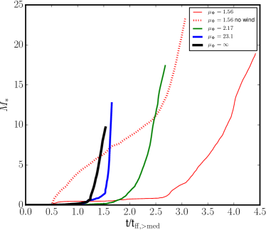
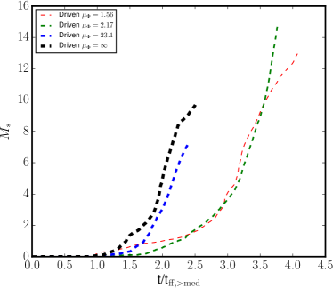
Figure 1: Total mass accreted for the models without (left) and with (right) turbulent forcing.

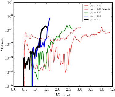
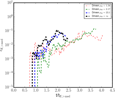
Figure 2: Instantaneous value of the dimensionless star formation rate $\epsilon_{\rm ff,>med}$ for the models without (left) and with (right) turbulent forcing (right). The data have been boxcar-smoothed over a timescale of $0.05~{}t_{\rm ff,>med}$ to remove short-timescale variability.

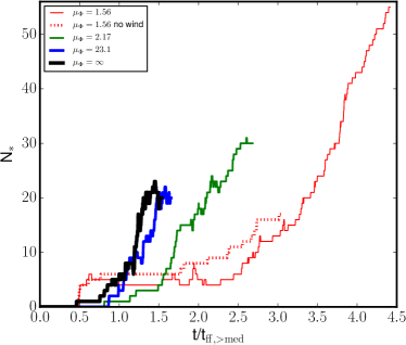
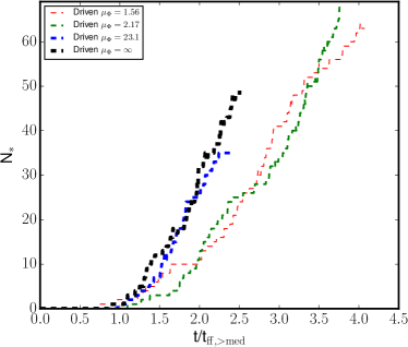
Figure 3: Total number of protostars formed for the models without (left) and with (right) turbulent forcing.

$\mu_{\Phi}$	Outflows	Driving	$\epsilon_{\rm ff,IC}$	$\epsilon_{\rm ff,>med}$	$\epsilon_{\rm ff,>0.8}$
$\mu_{\Phi}=1.56$	Y	N	12%	8.2%	6.0%
$\mu_{\Phi}=1.56$	N	N	23%	15.8%	19%
$\mu_{\Phi}=1.56$	Y	Y	4.8%	3.2%	4.2%
$\mu_{\Phi}=2.17$	Y	N	26%	18.8%	19%
$\mu_{\Phi}=2.17$	Y	Y	15%	11.0%	8.7%
$\mu_{\Phi}=23.1$	Y	N	$\gtrsim 30\%$	$\gtrsim 24\%$	$\gtrsim 22\%$
$\mu_{\Phi}=23.1$	Y	Y	8.2	6.4%	6.6%
$\mu_{\Phi}=\infty$	Y	N	$\gtrsim 50\%$	$\gtrsim 34\%$	$\gtrsim 37\%$
$\mu_{\Phi}=\infty$	Y	Y	6.0%	4.0%	5.2%

Table 2: Star formation efficiency per free fall time in each run. The various values of $\epsilon_{\rm ff}$ are computed for different definitions of the free-fall time, as discussed in Section 2.2. The quantities reported are averaged over the last $0.5t_{\rm ff,>med}$ of each simulation. A value preceded by $\gtrsim$ indicates that $\epsilon_{\rm ff}$ was still rising strongly and the end of the simulation, and the values listed are therefore lower limits.

3.2 Cluster Morphology

Figure 4 shows the mean density along lines of sight in the $\hat{{\bf x}}$ direction at the termination time of each model, overlaid with a semi-transparent rendering of regions with $|v|>2~{}v_{\rm rms}$. Recall that the initial magnetic field is in the $\hat{{\bf z}}$ direction, and is therefore upwardly oriented on the page in Figure 4. We note that the mean density along the line of sight, which is proportional to the surface density, becomes increasingly filamentary as the strength of the magnetic field increases. In the cases where the magnetic field is the most dynamically significant, the outflows are oriented predominately perpendicularly to the orientation of the densest structures. The $\mu_{\Phi}=1.56$ case with decaying turbulence indicates a final cluster geometry that is most dominated by the magnetic field. In this case, the cluster is arranged mostly in a planar geometry normal to the $\hat{{\bf z}}$ direction. The magnetic fields in this case are strong enough to constrain large-scale collapse to be predominantly in the direction of the initial magnetic field, with less harassment from large-scale turbulent forcing than the equivalent model with turbulent forcing.

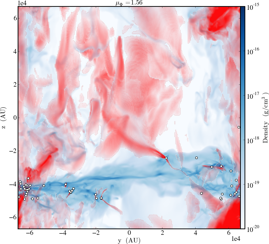
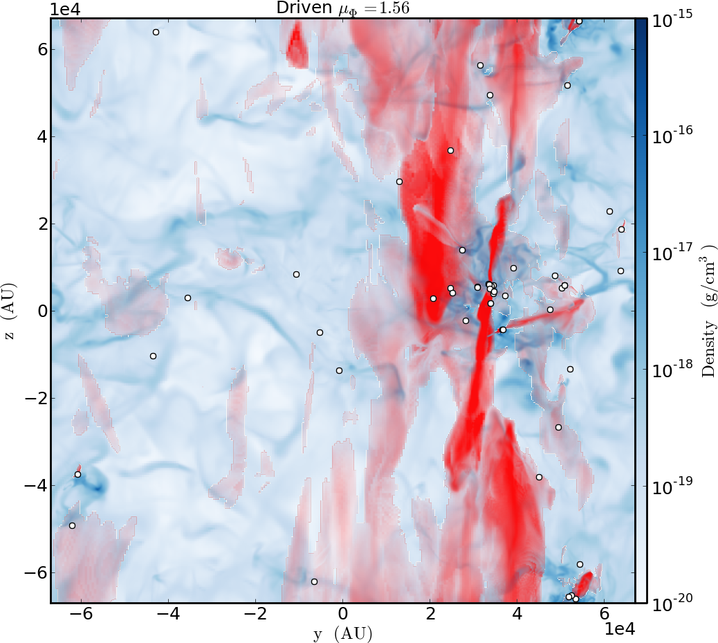
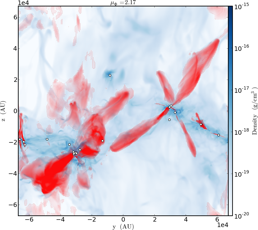
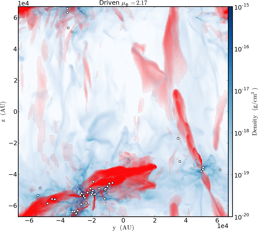
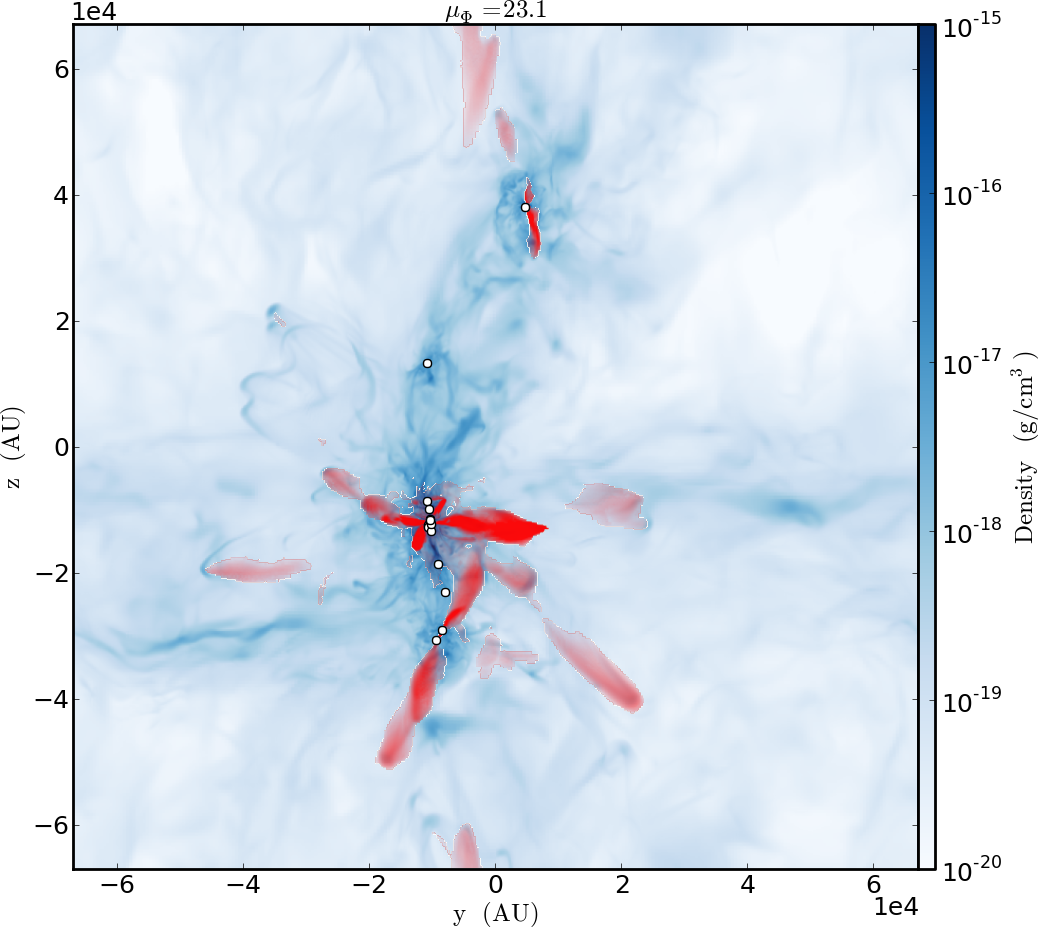
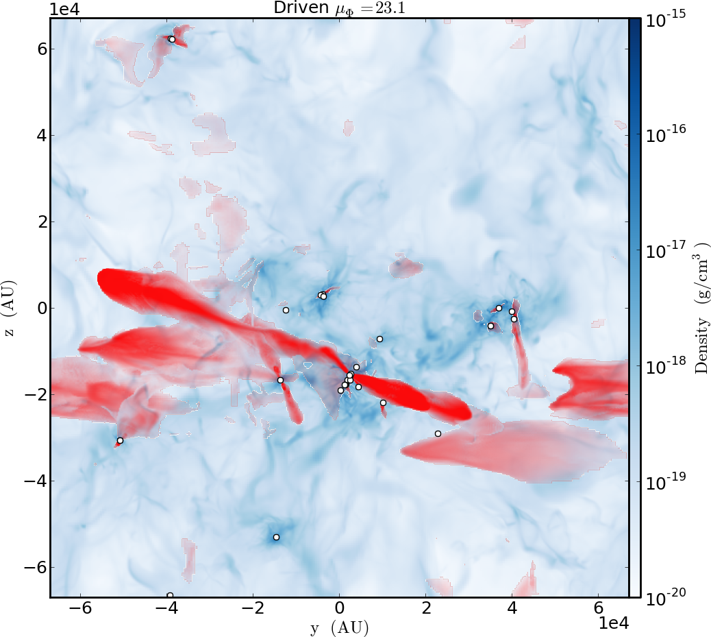
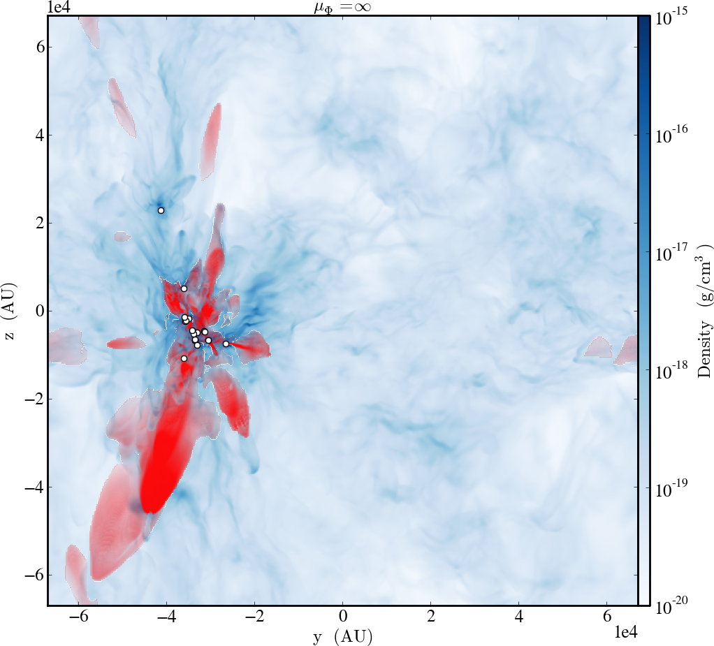
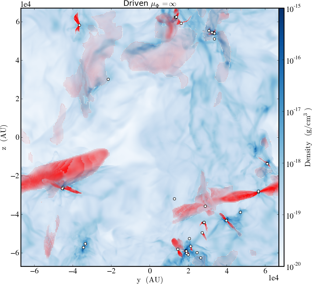
Figure 4: Volume-weighted mean densities projected along the $\hat{{\bf x}}$ direction for the models with turbulent forcing (right) and with decaying turbulence (left). The column density can be recovered by multiplying the mean density shown by the computational domain length $0.65~{}{\rm pc}$; for reference, this means that a density of $10^{-18}$ g cm^-3 corresponds to a column density of $2.0$ g cm^-2. The four rows show the $\mu_{\Phi}=1.56$, $\mu_{\Phi}=2.17$, $\mu_{\Phi}=23.1$, and $\mu_{\Phi}=\infty$ runs, from top to bottom. Regions with gas velocity greater than $2v_{\rm rms}$ are shaded in red with the opacity of the red regions increasing to a maximum for velocities exceeding $5v_{\rm RMS}$. White circles indicate the projected position of the protostellar sink particles.

3.3 Protostellar Mass Functions

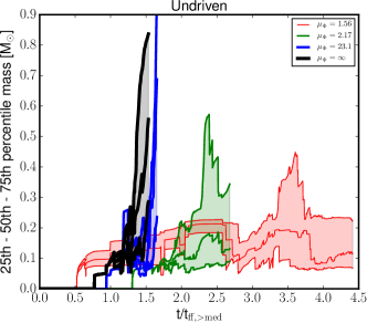
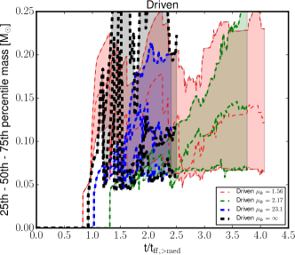
Figure 5: The evolution of the stellar mass distribution for models with turbulent forcing (right) and with decaying turbulence (left). In these figures, the central lines show the 50^th percentile mass, while the shaded regions indicate the $25^{\rm th}-75^{\rm th}$ percentile range. Colours correspond to different values of $\mu_{\Phi}$, as indicated in the legend.

We next examine the mass functions for the stars formed in our simulations. As a first step to this, we verify that these distributions have come close to being stable in time. To demonstrate this, in Figure 5 we plot the temporal evolution of the $25^{\rm th}$ percentile, median and $75^{\rm th}$ percentile of the distribution of protostellar masses in each model as a function of time. Similar to the temporal evolution of $\epsilon_{\rm ff}$, we see that the protostellar mass percentiles have mostly stabilised by the end of the runs, except for the cases of a weak initial field ($\mu_{\Phi}=23.1$ and $\infty$) with decaying turbulence. Consequently, we can interpret the protostellar mass distributions of the moderate and strong initial field models with decaying turbulence, and all of the models with driven turbulence, as being only weakly time-dependent. We do warn, however, that this stabilisation is a result of an equilibrium between new stars forming at low mass, and existing stars growing. As noted in Krumholz et al. (2016), if some process were to halt the formation of new stars but the existing stars were to continue accreting their envelopes, the mass distribution would shift upward.

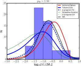
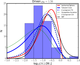
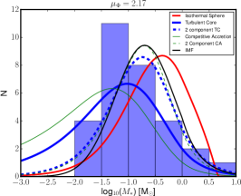
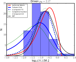
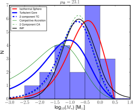
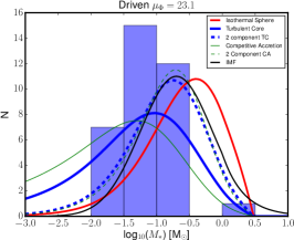
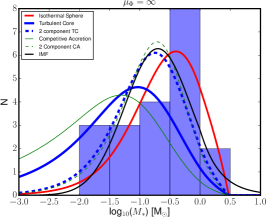
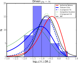
Figure 6: Histograms of protostellar masses at the end of each of the models with turbulent forcing (right) and with decaying turbulence (left). The four rows show the $\mu_{\Phi}=1.56$, $\mu_{\Phi}=2.17$, $\mu_{\Phi}=23.1$, and $\mu_{\Phi}=\infty$ from top to bottom. The black line shows the observed initial mass function (Chabrier, 2005). The other curves denoted in the figure legend show the analytic protostellar mass functions of McKee & Offner (2010) for the single and two component turblent core models, the single and two component competetive accretion models and the isothermal sphere model.

Figure 6 shows the protostellar mass distributions at the termination of each model. The black curve in the figure shows the observed initial mass function of (Chabrier, 2005). The mass distributions in our models have stabilized over dynamical timescales ($t_{\rm ff,>med}$), as shown in figure 5. However, because the sources in our models are still accreting, our models are not exactly comparable to the initial mass function that is representative of the distribution of final stellar masses. For this reason, we also compare our models to the protostellar mass functions (PMFs) from the analytic theory of McKee & Offner (2010); these PMFs are the mass distributions that one expects a series of protostars to possess if their final mass distribution matches the Chabrier (2005) IMF, and if the numbers of stars formed versus time $N_{*}(t)$ and the accretion histories of individual stars follow some specified functional form. We observe that $N_{*}(t)$ is a roughly linear function in all simulations except those that display runaway collapse, and thus we adopt a linear function for $N_{*}(t)$. For the accretion rate versus time of individual protostars, McKee & Offner (2010) consider a range of cases, all of which we plot together with the simulation results in Figure 6: competitive accretion (CA), turbulent core (TC), 2-component competitive accretion (2CCA), and 2-component turbulent core (2CTC); the latter two both approach the constant accretion rate expected for an isothermal sphere for low mass sources (IS), and we also plot the pure IS case. The only other parameter required by the McKee & Offner (2010) PMF analytic model is the upper limit to the most massive star that will form in the cluster $m_{\rm u}$. We have generated the theoretical PMFs in Figure 6 by setting $m_{\rm u}$ to the larger of $3~{}{M}_{\mathord{\odot}}$ or the value of $m_{\rm u}$ necessary so that the theoretical PMF has exactly one source heavier than the second-most massive particle present in the at the termination of the simulation. The choice of $m_{\rm u}$ largely affects the shape of the high-mass tail of the PMF and the conclusions that follow from comparing our simulation to the theoretical PMFs are insensitive to this choice. The $p$-value of the Kolmogorov-Smirnov (K-S) statistic comparing each simulation to each mass function is reported in table 3. The relative disagreement between simulations and mass functions pairs with $p$-values less than 0.05 is unlikely due to random chance. These distribution pairs are different with high statistical confidence. We denote the $p$-value of these pairs in bold text in the table.

Comparison Analytic Model	IMF	TC	2CTC	CA	2CCA	IS
$\mu_{\Phi}=1.56$	3.2$\times 10^{-4}$	0.094	1.7$\times 10^{-3}$	0.69	1.0$\times 10^{-3}$	1.1$\times 10^{-7}$
$\mu_{\Phi}=1.56$ No Wind	1.1$\times 10^{-3}$	7.7$\times 10^{-5}$	1.0$\times 10^{-3}$	6.0$\times 10^{-6}$	4.4$\times 10^{-4}$	0.054
$\mu_{\Phi}=2.17$	0.19	0.92	0.27	0.56	0.25	0.013
$\mu_{\Phi}=23.1$	0.058	4.2$\times 10^{-3}$	0.014	1.1$\times 10^{-3}$	9.9$\times 10^{-3}$	0.35
$\mu_{\Phi}=\infty$	0.50	1.3$\times 10^{-3}$	0.011	1.4$\times 10^{-4}$	9.2$\times 10^{-3}$	0.35
$\mu_{\Phi}=1.56$ Driven	3.0$\times 10^{-3}$	0.52	0.13	0.91	0.080	2.1$\times 10^{-3}$
$\mu_{\Phi}=2.17$ Driven	3.5$\times 10^{-3}$	0.72	0.086	0.94	0.050	1.6$\times 10^{-4}$
$\mu_{\Phi}=23.1$ Driven	0.033	0.19	0.032	0.63	0.033	2.9$\times 10^{-5}$
$\mu_{\Phi}=\infty$ Driven	4.4$\times 10^{-3}$	0.43	0.036	0.60	4.4$\times 10^{-3}$	1.9$\times 10^{-5}$

Table 3: Kolmogorov Smirnov statistic $p$-values for the distribution of protostars in each simulation as compared to the observed IMF (Chabrier, 2005) and several analytical protostellar mass functions including the turbulent core (TC), 2 component turbulent core (2CTC), competitive accretion (CA), 2 component competitive accretion (2CCA) and the isothermal sphere models (McKee & Offner, 2010). Simulations that include turbulent forcing are denoted as “Driven” in the left column. The other models are the cases of decaying turbulence. Simulation to mass function pairs with $p$-values less than 0.05 can be confidently interpreted as a sample drawn from a different distribution than the given mass function. The $p$-value for these ”rejected” models is denoted in bold-face in the table.

We find that our runs with weak initial fields ($\mu_{\Phi}=23.1$ and $\infty$) and no driving have peak masses that exceed the observed mode of the IMF ($m_{*}=0.2~{}{M}_{\mathord{\odot}}$ – Chabrier, 2005), and that are continuing to rise (Figure 5), at the termination of the models. As discussed in Section 3.1, these models also approach a state of rapid, near global free-fall collapse, contrary to observational constraints. Furthermore, the shape of the mass distributions is closest to that of the IS case. The ever-increasing peak of the PMFs in these simulations appears to be a manifestation of the overheating problem identified by Krumholz, Klein, & McKee (2011), whereby values of $\epsilon_{\rm ff}$ close to unity produce such high accretion luminosities that fragmentation is strongly suppressed, leading to a mass function that shifts to ever-higher masses as collapse continues but no new stars can be created. Furthermore, these simulations have low K-S statistic $p$-values when compared against all analytic models except for the IS one.

In contrast, the moderate and strong initial field cases all achieve stable or slowly increasing median masses in the range $0.05{M}_{\mathord{\odot}}<m_{*}<0.15{M}_{\mathord{\odot}}$, independent of the presence of external turbulent forcing. All of the models with continuously driven turbulence also show stable peak masses independent of the strength of the initial magnetic field. At the termination of these models, the median masses lie between the analytically predicted peak masses for the single component competitive accretion (CA) and single component turbulent core accretion (TC) models of $0.05{M}_{\mathord{\odot}}$ and $0.095{M}_{\mathord{\odot}}$, respectively. Because of the median masses for the CA and TC models are close to those of the numerical simulations, these simulations also have high K-S $p$-values when compared to the CA and TC theoretical models. The shape of the mass functions are not amenable to reliably differentiating among the moderately magnetized models or the weakly magnetized models with continuous turbulent forcing to within the statistical limitations of the number of sources in these simulations.

Figure 7 shows the protostellar mass distribution at the termination of the strongly magnetized $\mu_{\Phi}=1.56$ without turbulent driving or protostellar outflow ejection. The effect of outflows on the protostellar mass distribution can be seen clearly by comparing this figure to the top left panel of Figure 6, which shows the undriven $\mu_{\Phi}=1.56$ model with outflows. Clearly omission of outflows leads to a significant increase in the typical stellar mass and very low K-S test $p$-values. This difference is partly due to direct removal of mass by the outflows, but this effect alone cannot explain the difference in mass distribution, partly because it is too large (a factor of $\gtrsim 10$ in mass), and partly because there is also a dramatic drop in the total number of stars when we turn off outflows, something that cannot easily be explained by mass ejection. Instead, the shift in the mass function here appears to result from the interaction between outflows and radiative heating. Outflows indirectly reduce the luminosity of individual stars by lowering their accretion rates (Krumholz, Klein, & McKee, 2012; Hansen et al., 2012; Myers et al., 2014), and create paths of reduced optical depth, allowing more efficient escape of radiation from the gas immediately around the protostars (Krumholz, McKee, & Klein, 2005; Cunningham et al., 2011). Due to the omission of these two effects in the no-outflow model, radiative heating is much more effective at suppressing fragmentation, leading to the production of fewer, much more massive stars. We showed in Section 3.1 that the strong initial magnetic support in the no-outflow model was sufficient to limit the star formation efficiency to values consistent with observation, but clearly the shape of the mass distribution of this model is not consistent with observation.

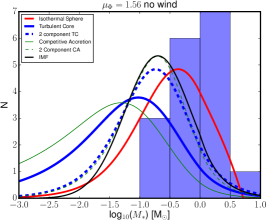
Figure 7: Histogram of the protostellar masses at the end of the $\mu_{\Phi}=1.56$ model without protostellar feedback.

It is also interesting to compare our results to previous simulations making use of a similar set of physical processes. Our $\mu_{\Phi}=1.56$ model with continuous driving is comparable to the recent models by Li, Klein, & McKee (2017); the simulations have similar initial ($\beta_{\rm IC}$ and $\mathcal{M}_{A,\rm IC}$) and post-driving ($\beta_{\rm>med}$, $\mathcal{M}_{A,\rm>med}$ and $\rho_{\rm>med}$) conditions. However, while in our case this model produces an IMF peak at slightly less than $0.1{M}_{\mathord{\odot}}$, the Li, Klein, & McKee (2017) simulations yield at peak at $0.2{M}_{\mathord{\odot}}$, comparable to the observed IMF peak. Given the similarities of the dimensionless conditions of the two cluster models, we attribute this difference to the outflow ejection parameters discussed in 2.3. The models presented here eject three times the momentum flux in the early phases of prestellar collapse and therefore have a more disruptive effects on their parent cores. While Cunningham et al. (2011) point out that observations do not precisely constrain the outflow model ejection parameters, the fact that the model in Li, Klein, & McKee (2017) achieves better agreement with the well-constrained median IMF suggests that the outflow ejection parameters used in that model are probably more realistic. This conclusion, however, does not affect the relative differences between the various runs that we have identified; indeed, a shift to higher masses as a result of somewhat weaker outflows would worsen the agreement between the observed IMF and those produced in the weakly-magnetised, non-driven models.

The other obvious prior work to which we can compare are the simulations of Hansen et al. (2012). Indeed, our non-magnetised, decaying turbulence model is identical to theirs apart from the random phases used during the initial turbulent driving phase. Both models ran for comparable times as well. However, the model presented in this work exhibits rapidly increasing accretion rates and commensurately increasing source masses at late time, while the simulations of Hansen et al. do not. While this might at first seem quite surprising, the result can be understood by examining Figure 1. This figure shows that the stellar mass at first increases relatively slowly, but then rapidly increases as the turbulence decays and free-fall collapse begins. The behaviour in the Hansen et al. simulation is consistent with what we see just before the onset of rapid collapse in our simulation. Since the exact time at which runaway collapse begins is almost certainly sensitive to the random driving, the most likely explanation for the difference is that the Hansen et al. simulation was simply not run quite long enough to reach the runaway collapse phase where the collapse begins to alter the IMF.

3.4 Stellar Multiplicity

The statistics of multiple systems provides another observational constraint against which our models can be tested. To compute the stellar system multiplicity we use the algorithm of Bate (2009). The algorithm works recursively: one identifies the most strongly bound pair of stars in the simulation, and replaces it with a single object at the centre of mass position of the pair with the total mass and momentum of its constituent protostars, then repeats until there are no more bound pairs that can be combined. In cases where combining the most bound pair of objects would create a system with a multiplicity greater than four, one skips it and combines the next-most bound combination instead. This is motivated by the fact that high-multiple bound systems are dynamically unstable and such systems are likely to break apart if the model were continued further in time. At the end of this procedure we obtain $S$ single star systems, $B$ binary systems, $T$ triple systems and $Q$ quadruple systems. For the set of bound systems the multiplicity fraction is defined as (Bate, 2009; Krumholz, Klein, & McKee, 2012; Myers et al., 2014)

$$\textrm{MF}=\frac{B+T+Q}{S+B+T+Q}$$ (13)

Figure 8 shows the multiplicity fraction as a function of the primary star mass in each of our simulations. Given the limited number of systems in at least some of our simulations, computing the multiplicity fraction requires some care. We do so in two ways. First, we form running averages, meaning that, for each primary star (i.e., single star or the most massive member of a multiple), we evaluate equation 13 for the set of systems consisting of that primary and the next most massive and next least massive primaries. This quantity is shown as the blue curve in Figure 8. Second, we can compute multiplicity in bins. To do so, we start with the least massive primary, and then place the primaries in bins of mass, with the bin width taken to be either sufficient to contain four primaries, or 0.2 dex, whichever is greater. For each bin, we regard the systems in it as samples drawn from a binomial distribution of multiples or singles, and from those samples we compute a central estimate and a 68% confidence interval on the true multiple system fraction in that bin (see Krumholz, Klein, & McKee 2012 for full details on how this computation is carried out). We plot the binned 68% confidence intervals as the shaded regions in Figure 8.

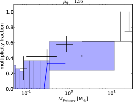
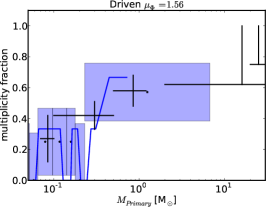
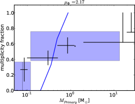
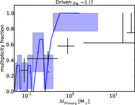
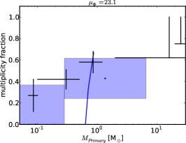
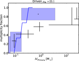
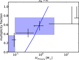
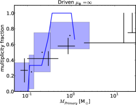
Figure 8: Multiple stellar system fraction at the end of each of the models with turbulent driving (right) and with decaying turbulence (left), computed as a function of primary star mass. The four rows show the $\mu_{\Phi}=1.56,2.17,23.1$, and $\infty$, from top to bottom. For the simulations, the blue curve indicates evolution of a running average over three systems as a function of mass, while shaded regions indicate the mean multiplicity and central 68% probability range on the multiplicity in bins – see main text for details on how the running average and binned values are computed. Black crosses denote the mass range and mean multiplicity found in observational surveys. The two highest mass surveys are statistical lower bounds. The horizantal marker on these observations indicate the lower bound. The observational data, from low to high mass, are compiled from Basri & Reiners (2006) and Allen (2007) (combined into the leftmost point), Fischer & Marcy (1992), Raghavan et al. (2010), Preibisch et al. (1999), Mason et al. (2009) and these are the same data used in Bate (2012) and Krumholz, Klein, & McKee (2012).

Comparing either the running averages or the binned results to the observed multiplicity fractions that we also plot in Figure 8, we find that all of the models generally agree with observations within the range of statistical uncertainties. It is noteworthy that the weakly magnetized models without turbulent forcing are consistent with observed multiplicity statistics even though their protostellar mass functions (3.3) are strongly inconsistent with observations. The driven turbulence $\mu_{\Phi}=2.17$ and $23.1$ models somewhat over-predict the multiplicity fraction for systems with primary mass $M_{p}\sim 1~{}{M}_{\mathord{\odot}}$, but this may be the result of poor statistics in this mass range in those models, and we note that the observational surveys are based on field stars, while there are strong hints that multiplicity fraction is higher for still-embedded systems (Tobin et al., 2016), which is the more relevant comparison for our simulations. We also note that, while the bins at low mass are generally consistent with the observations individually, taken together it is clear that we systematically under-produce multiple systems at low mass relative to the observational data. This is a likely a resolution effect. Our models do not resolve gas-particle gravity forces below the scale where sink source terms couple to the gas – $4\Delta x$. Low-mass multiple systems must necessarily be close and consequently more difficult to resolve to remain bound. This limitation is also noted in the multiplicity fractions extracted from the models of Bate (2009), Krumholz, Klein, & McKee (2012), and Myers et al. (2014).

3.5 Turbulent Decay and Protostellar Feedback Rates

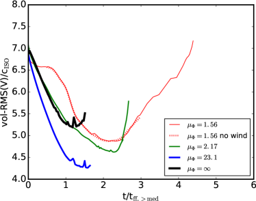
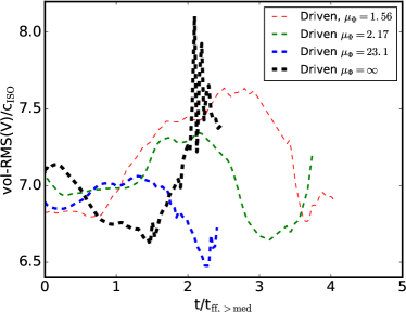
Figure 9: Volume-weighted root mean squared gas velocity, normalized by the gas sound speed, as a function of time for the models with turbulent forcing (right) and with decaying turbulence (left). Note the difference in scales between the left and right panels.

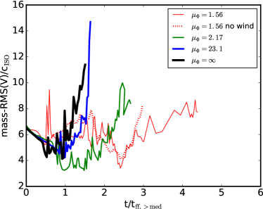
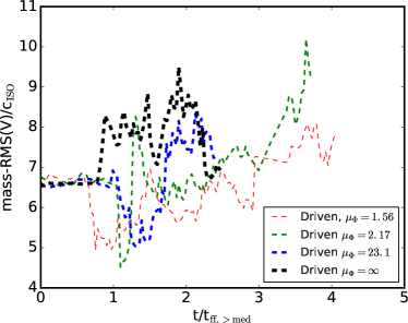
Figure 10: Same as Figure 9, but now showing mass-weighted rather than volume weighted velocities. As with Figure 9, note the difference in scales between the two panels.

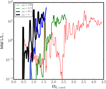
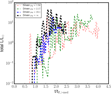
Figure 11: Total mechanical luminosity of the protostellar outflows as a function of time for the models with turbulent forcing (right) and with decaying turbulence (left). The data have been boxcar-smoothed with an interval of $0.05~{}t_{\rm ff}$.

Figure 9 shows the temporal evolution of the volume-weighted RMS gas velocity for each model. As intended, the models that include steady turbulent forcing remain within 10% of a constant RMS velocity with $\alpha_{\rm vir}\sim 1$. For the runs without driving, at early time, $t\lesssim t_{\rm ff}$, turbulent decay causes the RMS velocity to drop. However, after $1-2$ free-fall times (depending on the level of magnetic support) the system begins to undergo a global collapse, and this causes the velocity dispersion to rise again.

Figure 10 shows the temporal evolution of the mass-weighted RMS velocity dispersion. This averaging is more analogous to mass-biased observational line width-size measurements. However, it is also heavily biased toward dense, locally collapsing regions, which somewhat mutes the effect of turbulent decay relative to infall. Consequently, the clear drop in velocity dispersion seen in Figure 9 for the non-driven runs is absent here. We infer that mass-weighted line-width diagnostics are surprisingly insensitive to interruptions in large-scale driving source of durations up to $\la 1t_{\rm cross}$.

It is also interesting to compare the $\mu_{\Phi}=1.56$ cases with and without outflows. In principle the outflows have more than enough mechanical power to alter the turbulence. We illustrate this in Figure 11, which shows the outflow mechanical luminosity versus time, $L_{\rm outflow}=(1/2)\dot{M}_{\rm wind}v_{\rm wind}^{2}$. This is typically $\sim 1-10L_{\odot}$ at late times in our simulations, For comparison, the turbulent decay rate is $\sim\bar{\rho}v_{\rm rms}^{2}L^{3}/t_{\rm cross}\sim 10^{-3}~{}{L}_{\mathord{\odot}}$, roughly 3 orders of magnitude smaller. However, when we examine the volume-weighted RMS velocity, the $\mu_{\Phi}=1.56$ runs with and without outflows are nearly identical, and in the mass-weighted plot they are only slightly different. These results indicate that outflow mechanical power is efficiently dissipated by radiative shocks and does not quickly couple to the volume-filling turbulence of the surrounding molecular cloud, consistent with earlier works exploring the coupling of continuously driven jets through a stratified environments (Banerjee et al., 2007). What effects the outflows do have are limited to the dense gas surrounding protostellar cores, which is why the mass-weighted average shows an effect from outflows but the volume-weighted one does not. However, we emphasise that even in a mass-weighted sense the effect is modest. In our simulations, outflows do not appear to be efficient drivers of turbulence.

3.6 Local Magnetic Support

The turbulent driving phase introduces stretching and amplification of the magnetic field, relative to the initial magnetic field strength. The Alfvèn Mach number captures the strength of the turbulence relative to the initial magnetic field. As discussed in Section 2, the magnetized models in this work span the range $1<{\cal M}_{\rm A}<15$. However, the weakly magnetized models endure more significant stretching of the magnetic field and more small-scale magnetic field amplification in the turbulent driving phase than the more strongly magnetized models. The tangled magnetic field is further amplified due to collapse after self-gravity is switched on. Therefore, it is only the mean, large-scale field that is weak in our “weak-field” model. On the scale of the prestellar dense cores, the magnetic field is significantly more tangled and stretched than in stronger field models. Similar field amplification due to turbulence and the early gravitational collapse phase into starless dark clumps was noted in Li, McKee, & Klein (2015, section 8 in particular). In this section we examine the magnetic field structure in the vicinity of protostars, with the goal of understanding how the combination of turbulent and gravitational amplification maps from the initial, large-scale magnetic field to the final, small-scale one in the dense gas that is bound to and actively feeding accretion onto protostellar sources.

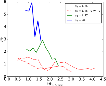
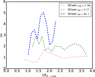
Figure 12: Temporal evolution of the mean mass-to-flux ratio averaged over the bound gas around each protostar. The averaging is weighted by protostellar mass. The plot is presented in units of the magnetically critical mass, for the models with turbulent forcing (right) and with decaying turbulence (left).

We seek to characterize the mean mass-to-flux ratio, averaged over the bound gas around each protostar that is poised for imminent accretion. We take this gas to be that which satisfies the condition

$$\frac{({\bf v}-{\bf v_{*}})\cdot({\bf x}-{\bf x_{*}})}{|{\bf x}-{\bf x_{*}}|}+c_{s}<\sqrt{\frac{Gm_{*}}{|{\bf x}-{\bf x_{*}}|}},$$ (14)

where ${\bf x}$, ${\bf v}$ and $c_{s}$ are the position, velocity and sound speed of the gas in the computational domain and ${\bf x_{*}}$, ${\bf v_{*}}$ and $m_{*}$ are the position, velocity and mass of each protostar. This criterion selects gas with insufficient thermal or kinetic energy to escape eventual accretion to the protostar, but distinguishes between infalling gas (for which ${\bf v}-{\bf v_{*}}$ is anti-aligned with ${\bf x}-{\bf x_{*}}$, and thus the dot product is negative), which is more bound, and outflowing gas (vectors aligned), which is less so. We assign gas that is bound to more than one star under this criterion only to the star to which it is most strongly bound.

For each star $i$, we have now defined a mass $m_{{\rm gas},i}$ of “bound gas." We next compute the volume weighted mean magnetic field direction in this gas, $\hat{\bf B}_{i}$, and we define the associated magnetic flux $\Phi_{i}$ as the net flux through the intersection of the plane defined by $\hat{\bf B}_{i}$ and the volume of assigned gas. Finally, we characterize the local mass-to-flux ratio of the gas assigned to each star as $\mu_{\Phi,i}=m_{{\rm gas},i}/M_{\Phi,i}$ where $M_{\Phi,i}$ is the magnetic critical mass computed from equation 1. It should be noted that the significance of $\mu_{\Phi}$ changes if a protostar is present in the cloud: The protostellar gravity also acts on the gas, so that accretion can occur normal to the field even for $\mu_{\Phi}<1$.

Figure 12 shows the temporal evolution of the mean mass-to-flux ratio averaged over the bound gas around each protostar. The average is weighted the by the mass of each protostar. Due to the computational burden associated with post-processing this result from our models, the plots in Figure 12 are sampled only every $0.2t_{\mathrm{ff,>med}}$ in time. In the figure, the curve for each model begins after the formation of the first sink particle.

In interpreting Figure 12 it is important to bear in mind that this diagnostic characterizes the net impact of multiple competing processes. Under our sink particle prescription (Lee et al., 2014), infalling gas is released from its associated magnetic flux the instant that it deposited onto the sink particle. This prescription is intended to mimic resistive effects near the surface of the protostar at length scales below that which can be resolved by our models. Consequently accretion causes the mass-to-flux ratio associated with locally bound dense gas clumps to decrease. The accreted mass is removed from the gas but the flux remains. However, the magnetic flux may subsequently escape, because it is no longer anchored to the gravitationally bound material – this is a form of magnetic interchange instability (Zhao et al., 2011; Krasnopolsky et al., 2012; Cunningham et al., 2012; Li et al., 2014). If the magnetic flux tubes escape the gravitationally bound region, this drives the mass to flux ratio back up. Similarly, turbulent magnetic reconnection acts to diffuse magnetic flux and increases the local mass-to-flux ratio in regions that undergo reconnection. In this case, the gas mass remains but the magnetic flux is displaced outward (Santos-Lima et al., 2012). Outflow ejection and turbulent forcing also impart mechanical energy to the system, and the resulting flows can further amplify, entangle, and ultimately reconnect magnetic flux tubes (Sur et al., 2012; Li, McKee, & Klein, 2015). In this way accretion, outflow, field tangling and reconnection all influence the mass to flux ratio. Since accretion itself is episodic, so too is the evolution of the mean mass to flux ratio of the bound gas in Figure 12. We anticipate the degree of tangling and episodic reconnection to be most pronounced in the weak-field models as weaker fields are more readily tangled and amplified by the turbulent flow. This too is borne out in Figure 12.

In the undriven models shown in the left panel of Figure 12, the mass-to-flux ratios in the bound gas systematically decreases with time for each of the models. This indicates that buoyant flux tubes rising away from the protostars as a consequence of accretion act enhance the degree of magnetic support to the bound gas, and this enhancement overwhelms the effect of turbulent reconnection. The $\mu_{\Phi}=1.56$ model without outflows indicates systematically stronger magnetic support in bound gas than the case with outflows. This indicates that outflows contribute to magnetic reconnection and consequent outward transport of magnetic flux, and explains why these models achieve comparable star formation efficiency ($\epsilon_{\rm ff,IC}=12\%$ in the case without outflows and $\epsilon_{\rm ff,IC}=23\%$ in the case with outflows). The enhanced magnetic support in the case without outflows offsets the loss of mechanical feedback support when the outflows are turned off. The $\mu_{\Phi}=2.17$ model is also strongly magnetically supported, with the mass-to-flux ratio in the bound gas approaching $\mu_{\Phi}\sim 1$ at late time, consistent with its accretion rate $\epsilon_{\rm ff,IC}=14\%$, slightly higher than the more strongly magnetized $\mu_{\Phi}=1.56$. The model that began with a field characterized globally as $\mu_{\Phi}=23.1$ attains a characteristic mass-to-flux ratio $\mu_{\Phi}\approx 5$ via field amplification and gravitational compression by the time the first protostellar particle forms. While the level of magnetic support in the bound gas increases with time, the degree of magnetic support achieved by the end of the model is insufficient to significantly reduce the net accretion rate from that of the purely hydrodynamical case.

The evolution of the mass-to-flux ratio of the bound gas in the models with driven turbulence models is shown in the right panel of Figure 12. In this case the model that began with a global $\mu_{\Phi}=2.17$ retains a roughly constant mass-to-flux ratio in the bound gas of $\mu_{\Phi}\sim 2$ throughout its evolution. The model that began with a global $\mu_{\Phi}=1.56$ attains stronger magnetic stabilization in the dense gas with $\mu_{\Phi}<1$ by the time the first protostars have formed. Subsequent evolution indicates a slowly decreasing level of magnetic support in the bound gas, stabilizing to $\mu_{\Phi}\gtrsim 1$. The model that began with a global $\mu_{\Phi}=23.1$ enhances the degree of magnetic support in the bound gas with time, reaching to $\mu_{\Phi}\sim 4$ by the end of the model.

Taken in aggregate, our results indicate that small-scale dissipation effects near the surface of a protostar provide a feedback loop for stabilising the star formation efficiency. Bound gas cores that are under-supported initially undergo more rapid collapse than cores that are better supported, independent of whether the initial support is predominately turbulent or magnetic. The more rapidly collapsing regions reconnect and expel magnetic flux to the core from the newly-formed protostar at a faster rate. The end result of this process over a time scale $>1t_{\textrm{ff}}$ is that cores with continuous mechanical support that remain in near virial equilibrium approach mass-to-flux ratios of $\mu_{\Phi}<5$ independent of the large-scale mean field strength. Models with decaying or otherwise sub-virial levels of turbulent support will lead to greater local enhancement of the level of magnetic support in the bound gas, approaching $\mu_{\Phi}<2$ at late time.

4 Magnetic and Radiative Effects in Shaping the IMF

In Section 3.3 we demonstrated that our models have protostellar mass distributions that are stable or evolving slowly toward higher mass only slowly compared to cloud-collapse timescales. The models with weak initial fields or a lack of driving all have median masses that are too large in comparison to the observed IMF, while the strong field and driven cases have smaller median masses that are at least roughly compatible with these models reproducing the observed IMF. It is therefore interesting to investigate in more depth what mechanisms shape this mass distributions. To explore this question, we turn to the techniques described in Krumholz et al. (2016), who analysed the simulations of Myers et al. (2014); these simulations use the same physics we include here, but focus on a much denser region appropriate to sites of high mass star formation. Comparing the two sets of simulations therefore enables us to understand how this question depends on the star-forming environment.

4.1 Analysis Methodology

We begin with a brief summary of the Krumholz et al. (2016) analysis, and refer readers interested in the details to that paper for a full description. The central idea of this analysis is to determine what physical process is responsible for halting fragmentation in the vicinity of each protostar, thereby leaving the mass available for accretion and the build up of more massive stars, rather than the production of additional low mass stars. To this end, we examine spherical regions of gas within a $4000~{}{\rm AU}$ radius around each protostellar sink particle at time intervals of $0.05t_{\rm ff,>med}$. We divide the volume of interest into 128 spherical shells of radius $r$ concentric with the position of the sink particle. For each shell, we compute the total gas enclosed $m_{\rm gas}$, excluding the sink particle mass, the mean density $\rho$ of the enclosed material, and its mass-weighted mean sound speed $c_{s}$. From the resulting profiles in $\rho$ and $c_{s}$ we compute an effective temperature

$$T_{\rm eff}=\frac{\mu m_{H}}{k_{B}}c_{s}^{2},$$ (15)

and, more importantly from the standpoint of determining whether gas will fragment, the Bonnor-Ebert mass (Ebert, 1955; Bonnor, 1956),

$$m_{\rm BE}=1.86\sqrt{\frac{c_{s}^{3}}{G^{3}\rho}}.$$ (16)

The Bonnor-Ebert mass characterizes the degree of thermal support. Absent other forces, objects less massive than $m_{\rm BE}$ are stable against collapse and objects more massive than $m_{\rm BE}$ are unstable against collapse. To elucidate the importance of heating by protostars in stabilizing the core, we repeat the computation with the sound speed $c_{s}=0.19~{}\textrm{cm s}^{-1}$, the sound speed of molecular gas at $10~{}\textrm{K}$ used as the background isothermal temperature in the simulations. We shall denote this quantity as $m_{\rm BE,10}$. Comparison of $m_{\rm BE}$ with $m_{\rm BE,10}$ enables us to determine the importance of radiative heating in limiting fragmentation.

To characterise the importance of magnetic forces, we compute the magnetic flux $\Phi$ threading each spherical shell, defined so that $\Phi=\int|{\bf B}\cdot\hat{n}|\,d^{2}x$ is computed along a circular cross section that is concentric with the spherical shell and has normal $\hat{n}$. The absolute value is taken in the integration on the assumption that oppositely-directed fluxes do not reconnect and cancel. We consider 12 possible orientations for $\hat{n}$, uniformly distributed on the unit sphere, with one value aligned with the star’s angular momentum vector, and use the largest value of $\Phi$ we find for all the $\hat{n}$ values considered. From this we can compute an effective mean magnetic field strength inside a radius $r$,

$$B_{\rm eff}(<r)=\frac{\Phi}{\pi r^{2}},$$ (17)

a magnetic critical mass $m_{\Phi}$ (equation 1), and the magnetically-supported mass (Mouschovias & Spitzer, 1976; McKee & Ostriker, 2007)

$$m_{B}=\frac{m^{3}_{\Phi}}{m^{2}_{\rm gas}}.$$ (18)

We prefer $m_{B}$ to $m_{\Phi}$ for this analysis as the former is an intensive quantity that does not depend on the size of the volume considered.

It has been well established that magnetic fields influence the spectrum of stars formed and reduce the star formation efficiency (Price & Bate, 2008). Here, we elucidate the relative contribution or radiative feedback to magnetic support by comparing the enclosed mass $m_{\rm gas}$ with the thermally- and magnetically-supported masses $m_{\rm BE}$ and $m_{B}$. This provides direct insight into the role of thermal support (augmented by radiative heating) and magnetic fields in shaping the IMF. For sufficiently small shells around each protostar, we always find $m_{\rm gas}\ll m_{\rm BE}$ and $m_{\rm gas}\ll m_{B}$, i.e., the enclosed mass is too small to fragment and form another star given the level of thermal and magnetic support. This gas will almost certainly be accreted onto the star that it surrounds, augmenting this star’s mass. At sufficiently large radii, $m_{\rm gas}\gg m_{\rm BE}$ and $m_{\rm gas}\gg m_{B}$, i.e., the mass enclosed is large enough that is able to fragment and produce additional stars, rather than being accreted onto the star it surrounds. Thus the shell at which $m_{\rm gas}\approx\max(m_{\rm BE},m_{B})$ marks a rough dividing line between gas that will end up in the existing star and gas that will end up elsewhere, and $m_{*}+m_{\rm gas}$ provides a rough estimate of the mass to which the star is likely to grow. We define the thermal critical mass $m_{\rm BE,crit}$ as the smallest (and almost always sole) mass where $m_{\rm gas}=m_{\rm BE}$, and analogously for $m_{B,{\rm crit}}$ and $m_{\rm BE,10,crit}$. Thus these critical masses provide a rough estimate of the future mass supply available for each star.

Krumholz et al. (2016) show that, in the simulations of Myers et al. (2014), stars with mass $m_{*}\ll 0.2$ $M_{\odot}$ almost invariably have stabilised gaseous envelopes such that $m_{\rm BE,crit}\gg m_{*}$, explaining the relative rarity of brown dwarfs as compared to stars: brown dwarf mass fragments can form, but when they do, they stabilise enough gas around themselves that they usually continuing accreting well out of the brown dwarf mass regime. Moreover, Krumholz et al. (2016) find that their stabilised regions have $m_{\rm BE,crit}\gg m_{B,{\rm crit}}\gg m_{\rm BE,10,crit}$, indicating that, while magnetic support is more important than thermal support in the absence of radiative heating, once one considers the effects of stellar radiation, it is the dominant factor in limiting fragmentation and thus establishing the location of the IMF peak.

4.2 Profiles of Mean Density, Temperature and Magnetic Field

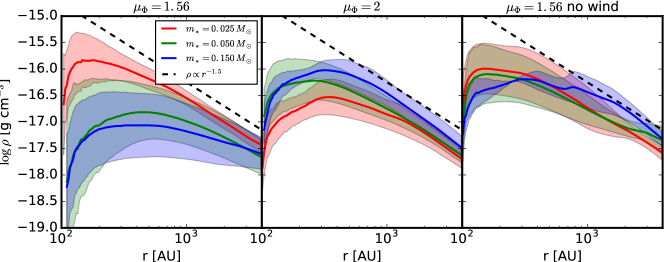
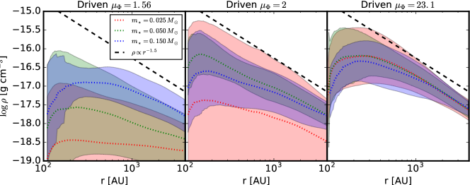
Figure 13: Mean density profiles $\rho(r)$ averaged in spherical shells around protostars. The panels shows the results for the strong (left), moderate (centre) and weak (right) magnetic field models. The top row depicts results for the models without turbulence driving after the onset of self-gravity at $t=0$. The bottom row depicts results for the model with continued turbulence driving after the onset of self-gravity. Different colours show means for protostars of mass $0.025~{}{M}_{\mathord{\odot}}$, $0.05~{}{M}_{\mathord{\odot}}$ and $0.15~{}{M}_{\mathord{\odot}}$. For each mass bin, the central line shows the mean while the shaded band shows the $1~{}\sigma$ dispersion for protostars in that mass bin. The dashed black line shows the density scaling $\rho\propto r^{-3/2}$, expected for free-fall collapse.

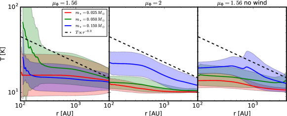
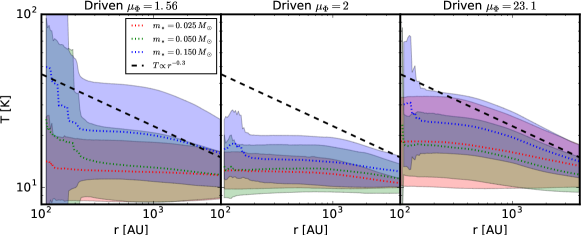
Figure 14: Same as Figure 13 but showing the mean effective temperature $T_{\rm eff}(r)$ (equation 15). The black dashed line shows a $T_{\rm eff}\propto r^{-0.3}$. The initial temperature of the models is $T=10~{}{\rm K}$.

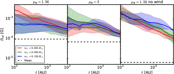
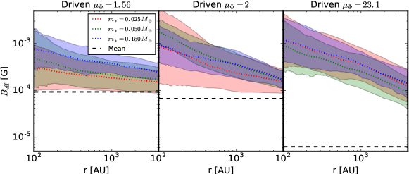
Figure 15: Same as Figure 13 but showing the mean effective magnetic field $B_{\rm eff}(<r)$ (equation 17). The black dashed horizontal line indicates the initial magnetic field strength before driving to the initial turbulent state.

Figure 13 shows the average density profile around central stars with three different masses; the averages plotted are taken over all protostars at all times. The density profiles always show a central dip at $130~{}\textrm{AU}<r<260~{}\textrm{AU}$, which is a result of our sink particle accretion zones; we therefore ignore this region in our analysis. At larger radii, we find that the moderately and weakly magnetized models ($\mu_{\Phi}\geq$ 2) without driving have density profiles $\rho\propto r^{-3/2}$. This profile is consistent with that expected for free-fall collapse onto a point mass. However, for Bondi-type flow the density at a fixed distance from the central object should increase with mass. The fact that it does not is inconsistent with pure Bondi flow, but is consistent with the turbulent core model of McKee & Tan (2003) and with the model of Murray et al. (2015) for the for collapsing, self-gravitating, turbulent cores. In contrast, the strongly magnetized ($\mu_{\Phi}=1.56$) undriven cases, and all driven cases for a central star mass of $m_{*}=0.15~{}{M}_{\mathord{\odot}}$, show slightly shallower density profiles. This is consistent with a buildup of magnetic flux resulting in a slower than free-fall collapse.

Figure 14 shows averaged profiles of $T_{\rm eff}$. Except for the $\mu_{\Phi}=1.56$ undriven model, these profiles indicate increasing $T_{\rm eff}$ with central star mass. As Krumholz et al. (2016) point out, to maintain a constant density profile, infall velocities and accretion rate must increase as the progenitor mass increases. Since accretion luminosity is the dominant source of radiative heating in low mass sources, the temperature around them rises with their mass. The weakly magnetized models show the most rapid increase in heating with mass. Krumholz et al. (2016) noted a similar trend in models of denser high mass star forming regions, and also found that the temperature profiles were always close to $T_{\rm eff}\propto r^{-0.3}$. Here we find substantially shallower profiles, likely because the lower optical depth environment we are simulating is less effective at trapping the radiation (Krumholz & McKee, 2008).

In Figure 15 we show the corresponding average profiles of $B_{\rm eff}$. Consistent with our findings in Section 3.6, despite the large differences in large-scale magnetic flux, there is very little difference between the small-scale magnetic field strengths around protostars in the different simulations. Nor does the effective field strength increase with star mass, as one might expect from a naive picture in which accretion drags magnetic flux toward a star.

The non-dependence of the small scale magnetic fields on either the large-scale flux or the amount of gas that has already been accreted strongly suggests that the magnetic field profiles we find are the result of a self-regulation mechanism operating on small scales. We can think of this self-regulation as due to two pairs of competing processes, although given our limited resolution and the complex nature of the flows in our simulations, we cannot easily identify which mechanisms dominate. First, there is a competition between dynamo amplification and reconnection. In a turbulent dynamo, magnetic fields amplify until these two effects balance (Sur et al., 2012; Li, McKee, & Klein, 2015). Second, there is a competition between advection and magnetic interchange instabilities. As gas accretes, magnetic flux tubes are advected into the cores around the protostars, which tends to drive up $B_{\rm eff}$. The countervailing process is escape of flux through magnetic interchange instabilities. In reality, the interchange instabilities are triggered by resistive effects close to the surface of the protostar, which decouple flux tubes from the mass that anchors them and allows them to drift outward (Zhao et al., 2011; Krasnopolsky et al., 2012; Cunningham et al., 2012; Li et al., 2014); we model this by not accreting any magnetic flux into the star particles. If the flux liberated from the protostar diffused out to a radius $R$, then it would contribute a mean field

$$B_{\rm eff,*}=2G^{1/2}\left(\frac{L}{Z}\right)\frac{m_{*}}{\mu_{\Phi}R^{2}},$$ (19)

where we have assumed that the protostar has formed from a cylinder of gas with a height $Z$ less than the box height $L$. For $m_{*}=0.15\,M_{\odot}$ and $\mu_{\Phi}=1.56$, the results in Figure 15 place a lower limit $R>1000$ au on the distance that the field has diffused outward.

4.3 Critical Mass

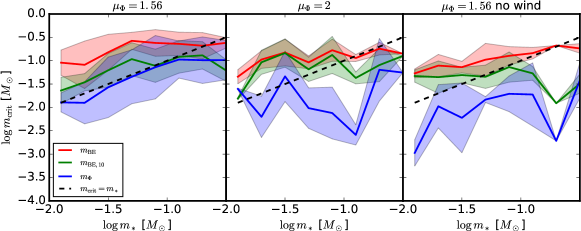
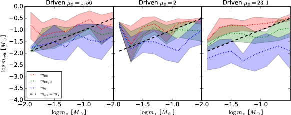
Figure 16: Critical mass of gas supported by thermal pressure $m_{\rm BE}$, thermal pressure fixed to the initial temperature $10~{}{\rm K}$ $m_{\rm BE,10}$ and magnetic fields $m_{B}$ as a function of central stellar mass $m_{*}$. Shaded bands indicate $1~{}\sigma$ dispersion over the protostars. The dashed black line indicates where the mass supported against collapse by pressure or magnetic forces is sufficient to double the present stellar mass, $m_{*}=m_{\rm crit}$. The panels shows the results for the strong (left), moderate (centre) and weak (right) magnetic field models. The top row depicts results for the models without turbulence driving after the onset of self-gravity at $t=0$.

In figure 16, we show the critical mass of gas supported by thermal pressure, $m_{\rm BE}$, thermal pressure fixed to the initial temperature, $10~{}{\rm K}$ $m_{\rm BE,10}$, and magnetic fields, $m_{B}$, as a function of central stellar mass $m_{*}$ as described in §4.2. When $m_{\rm crit}>m_{*}$, the mass of the stabilised envelope around a protostar is much greater than the mass of the star itself, and thus is likely to greatly increase its mass.

First consider thermal support. Krumholz et al. (2016) found that $m_{\rm BE}$ was typically a factor of $\sim 10$ larger than $m_{\rm BE,10}$, indicating that radiative heating increased the amount of mass that could be thermally supported by a factor of $\sim 10$. In our lower mass cluster models the difference between $m_{\rm BE}$ and $m_{\rm BE,10}$, is less pronouned, closer to $0.5$ dex than 1 dex. However, the difference is smaller not because $m_{\rm BE}$ is smaller, but rather because $m_{\rm BE,10}$ is larger. That is to say, in our lower density simulation the characteristic density is lower, and thus the Bonnor-Ebert mass in unheated gas is larger. In comparison, the mass that can be supported after heating, $m_{\rm BE}$, is almost unchanged and independent of environment—the increase in the temperature of the gas has been compensated by an increase in its density.

Next consider magnetic support. The results in Figure 16 are consistent with the findings of Krumholz et al. (2016) that the magnetic fields are relatively unimportant in supporting the cores compared to thermal pressure. Again, this points to the importance of local processes in regulating the magnetic field structure in the vicnity of protostars. The magnetic flux in the $\mu_{\Phi}=1.56$ case is sufficient to support a mass $m_{\Phi}=119~{}{M}_{\mathord{\odot}}$ against collapse, but the field threading the local region around the protostars is strong enough to support only $0.01~{}{M}_{\mathord{\odot}}$ to $0.1~{}{M}_{\mathord{\odot}}$. This result explains why the mode of the IMFs (§3.3) in our models are relatively insensitive to the large-scale magnetic field. The critical mass supported against fragmentation is determined primarily by thermal effects enhanced by radiation. Magnetic fields thus have a significant effect on the rate of star formation, but not on the IMF.

5 Conclusions

We present a numerical study of low-mass star cluster formation, and how this process is affected by the strength of the large-scale magnetic field, the presence or absence of turbulent energy input, and the effects of protostellar outflows. Our simulations include MHD, radiative transfer and protostellar radiation feedback, and protostellar outflows, a combination of physical processes that has received little attention in the literature to date.

Our primary finding is that our models are able to reproduce the observed (low) efficiency of star formation and the observed location of the IMF peak (to within a factor 2) only in models that include outflows and that do not undergo global collapse, either because they are supported by external energy input that drives the turbulence, or because they are close enough to the line of magnetic criticality for magnetic fields to inhibit collapse. In contrast, multiplicity statistics are insensitive to all variations in the initial conditions.

Krumholz, Klein, & McKee (2011, 2012) had previously conjectured that there might be a link between the low efficiency of star formation and the location of the IMF peak, but this was based on a single set of non-magnetised simulations. Our much more extensive suite of radiation-MHD simulations puts this conclusion on a much firmer footing, and suggests a general principle: the IMF peak location is directly linked to the inefficiency of star formation.

The primary mechanism controlling the IMF peak appears to be accretion-powered radiation from forming protostars, which produces enhanced thermal pressure on small scales in the vicinity of forming stars, as noted earlier by Bate (2009) as well. In comparison, the small-scale magnetic field structure around forming protostars is both insensitive to the large-scale magnetic field strength, and dynamically sub-dominant compared to radiation when it comes to regulating gas fragmentation. These results strongly favour a picture in which the small-scale magnetic field structure around protostars is regulated by local competitions between accretion of magnetized material and dynamo amplification, which tend to enhanced the field strength, and magnetic interchange instability and turbulent reconnection, which tend to suppress it. The competition between these processes tends to force the local mass to flux ratio in gas bound to protostars to $\sim 2$ (normalized to the critical value), regardless of the large-scale field.

Our models lack resolution to capture the effects of thermal support against gravitational contraction deep within very low mass cores and we lack non-ideal MHD effects that are most strongly coupled to turbulent density profiles on small scales. However these effects should influence our modeled protostellar mass distributions only on the low mass tail $m_{*}\lesssim 0.05{M}_{\mathord{\odot}}$ and our conclusions are not sensitive to these effects. We acknowledge that higher resolution models with non-ideal effects and multiple realizations to capture better statistics at protostellar mass extrema could improve the comparisons with observation made here by capturing a wider range of source masses with higher fidelity.

References

- Allen (2007) Allen, P. R. 2007, ApJ, 668, 492
- Banerjee et al. (2007) Banerjee, R., Klessen, R. S., & Fendt, C. 2007, ApJ, 668, 1028
- Basri & Reiners (2006) Basri, G., & Reiners, A. 2006, AJ, 132, 663
- Bate (2009) Bate, M. R. 2009, MNRAS, 392, 590
- Bate (2012) Bate, M. R. 2012, MNRAS, 419, 3115
- Bonnor (1956) Bonnor, W. B. 1956, MNRAS, 116, 351
- Crutcher et al. (2010) Crutcher, R. M., Wandelt, B., Heiles, C., Falgarone, E., & Troland, T. H. 2010, ApJ, 725, 466
- Chabrier (2005) Chabrier, G. 2005, The Initial Mass Function 50 Years Later, 327, 41
- Chakrabarti & McKee (2005) Chakrabarti, S., & McKee, C. F. 2005, ApJ, 631, 792
- Commerçon, Hennebelle, & Henning (2011) Commerçon, B., Hennebelle, P., & Henning, T. 2011, ApJ, 742, L9
- Cunningham et al. (2011) Cunningham, A. J., Klein, R. I., Krumholz, M. R., & McKee, C. F. 2011, ApJ, 740, 107
- Cunningham et al. (2012) Cunningham, A. J., McKee, C. F., Klein, R. I., Krumholz, M. R., & Teyssier, R. 2012, ApJ, 744, 185
- Ebert (1955) Ebert, R. 1955, Z. Astrophys., 37, 217
- Evans, Heiderman, & Vutisalchavakul (2014) Evans, II, N. J. and Heiderman, A. and Vutisalchavakul, N. 2014, ApJ, 782, 114
- Falgarone et al. (2008) Falgarone, E., Troland, T. H., Crutcher, R. M., & Paubert, G. 2008, A&A, 487, 247
- Federrath (2015) Federrath, C. 2015, MNRAS, 450, 4035
- Federrath & Klessen (2012) Federrath, C., & Klessen, R. S. 2012, ApJ, 761, 156
- Federrath, Klessen, & Schmidt (2009) Federrath, C., Klessen, R. S., & Schmidt, W. 2009, ApJ, 692, 364
- Federrath et al. (2010) Federrath, C., Roman-Duval, J., Klessen, R. S., Schmidt, W., & Mac Low, M.-M. 2010, A&A, 512, A81
- Federrath et al. (2011) Federrath, C., Sur, S., Schleicher, D. R. G., Banerjee, R., & Klessen, R. S. 2011, ApJ, 731, 62
- Feldmann & Gnedin (2011) Feldmann, R., & Gnedin, N. Y. 2011, ApJ, 727, L12
- Fischer & Marcy (1992) Fischer, D. A., & Marcy, G. W. 1992, ApJ, 396, 178
- Gammie & Ostriker (1996) Gammie, C. F., & Ostriker, E. C. 1996, ApJ, 466, 814
- García-Burillo et al. (2012) García-Burillo, S., Usero, A., Alonso-Herrero, A., Graciá-Carpio, J., Pereira-Santaella, M., Colina, L., Planesas, P., & Arribas, S. 2012, A&A, 539, A8
- Goldbaum et al. (2011) Goldbaum, N. J., Krumholz, M. R., Matzner, C. D., & McKee, C. F. 2011, ApJ, 738, 101
- Goldsmith (2001) Goldsmith, P. F. 2001, MNRAS, 557, 736
- Górski et al. (2005) Górski, K. M., Hivon, E., Banday, A. J., et al. 2005, ApJ, 622, 759
- Hansen et al. (2012) Hansen, C. E., Klein, R. I., McKee, C. F., & Fisher, R. T. 2012, ApJ, 747, 22
- Hennebelle et al. (2011) Hennebelle, P., Commerçon, B., Joos, M., et al. 2011, A&A, 528, A72
- Heyer et al. (2016) Heyer, M., Gutermuth, R., Urquhart, J. S., Csengeri, T., Wienen, M., Leurini, S., Menten, K., & Wyrowski, F. 2016, A&A, 588, A29
- Hubber & Whitworth (2005) Hubber, D. A., & Whitworth, A. P. 2005, A&A, 437, 113
- Klein et al. (1999) Klein, R. I., Fisher, R. T., McKee, C. F., & Truelove, J. K. 1999, Numerical Astrophysics, 240, 131
- Klessen & Hennebelle (2010) Klessen, R. S., & Hennebelle, P. 2010, A&A, 520, A17
- Krasnopolsky et al. (2012) Krasnopolsky, R., Li, Z.-Y., Shang, H., & Zhao, B. 2012, ApJ, 757, 77
- Krumholz (2014) Krumholz, M. R. 2014, Phys. Rep., 539, 49
- Krumholz (2015) Krumholz, M. R. 2015, arXiv:1511.03457
- Krumholz et al. (2010) Krumholz, M. R., Cunningham, A. J., Klein, R. I., & McKee, C. F. 2010, ApJ, 713, 1120
- Krumholz, Dekel, & McKee (2012) Krumholz, M. R., Dekel, A., & McKee, C. F. 2012, ApJ, 745, 69; Erratum 2013, ApJ, 779, 89