Multiscale analysis of the topological invariants in the logarithmic region of turbulent channels at $Re_{\tau}=932$

Abstract

The invariants of the velocity gradient tensor, $R$ and $Q$, and their enstrophy and strain components are studied in the logarithmic layer of an incompressible turbulent channel flow. The velocities are filtered in the three spatial directions and the results analyzed at different scales. We show that the $R$–$Q$ plane does not capture the changes undergone by the flow as the filter width increases, and that the enstrophy/enstrophy-production and strain/strain-production planes represent better choices. We also show that the conditional mean trajectories may differ significantly from the instantaneous behavior of the flow since they are the result of an averaging process where the mean is 3-5 times smaller than the corresponding standard deviation. The orbital periods in the $R$–$Q$ plane are shown to be independent of the intensity of the events, and of the same order of magnitude than those in the enstrophy/enstrophy-production and strain/strain-production planes. Our final goal is to test whether the dynamics of the flow are self-similar in the inertial range, and the answer turns out to be no. The mean shear is found to be responsible for the absence of self-similarity and progressively controls the dynamics of the eddies observed as the filter width increases. However, a self-similar behavior emerges when the calculations are repeated for the fluctuating velocity gradient tensor. Finally, the turbulent cascade in terms of vortex stretching is considered by computing the alignment of the vorticity at a given scale with the strain at a different one. These results generally support a non-negligible role of the phenomenological energy-cascade model formulated in terms of vortex stretching.

1 Introduction

The understanding of the structure of turbulence has been at the core of turbulence research from its very beginning. It is natural to investigate the gradients of the velocity, which provide important information regarding the local behavior of the flow. The invariants of the velocity gradient tensor for incompressible flows, $R$ and $Q$, were first introduced by Chong et al. (1990) and have proved to be a useful tool to analyze turbulent flows characterized by a wide range of scales (Chong et al., 1990; Chertkov et al., 1999; Chacin & Cantwell, 2000; Tanahashi et al., 2004; Chevillard & Meneveau, 2006; Lüthi et al., 2009; Atkinson et al., 2012; Wang & Lu, 2012; Cardesa et al., 2013). They quantify the relative strength of enstrophy production and strain self-amplification, and of local enstrophy density and strain density, respectively. Moving locally with a fluid particle, the velocity gradient tensor determines the linear approximation to the local velocity field surrounding the observer. In that frame, invariants can also be used to classify the local flow topology (Chong et al., 1990). However, the invariants are gradients of the velocities and hence, are dominated by the effect of the small scales. By filtering the velocity field, we will apply the topological and physical tools provided by the invariants to scales in the inertial range.

Measurements and simulations in different turbulent flows showed that the joint probability density function of $R$ and $Q$ has a very particular skewed ‘tear-drop’ shape, e.g. Soria et al. (1994); Ooi et al. (1999); Chertkov et al. (1999); Chacin & Cantwell (2000). That is, there is an increased probability of points where $R>0$ and $Q<0$ along the so-called Vieillefosse tail, reflecting a dominance of strain self-amplification over enstrophy production in strain-dominated regions. Such a signature turns out to be a quite universal feature persistent in many different turbulent flows, including mixing layers (Soria et al., 1994), channel flows (Blackburn et al., 1996), boundary layers (Chong et al., 1998; Atkinson et al., 2012), isotropic turbulence (Martín et al., 1998; Ooi et al., 1999), etc.

A better insight is gained by decomposing the velocity gradient tensor into its rate-of-rotation and rate-of-strain tensors (Blackburn et al., 1996; Chong et al., 1998; Ooi et al., 1999) or into their strain and enstrophy contributions (Gomes-Fernandes et al., 2014). Lüthi et al. (2009) expanded the $R$–$Q$ plane to three dimensions and studied the effect of enstrophy production and strain self-amplification separately using direct numerical simulations (DNSs) of isotropic turbulence at a Taylor-based Reynolds number $Re_{\lambda}=434$.

Martín et al. (1998) and Ooi et al. (1999) introduced and studied the conditional mean trajectories of the invariants (henceforth, CMTs) in DNSs of isotropic turbulence at $Re_{\lambda}=40$-$70$. This involved the calculation of the mean temporal rate of change along the fluid particle trajectories of the invariants conditioned on the values of the invariants themselves, which results in a vector field in the $R$–$Q$ plane. The resulting conditional vector field can be integrated to produce trajectories within the space of the invariants.

The analysis of the CMTs provides information about the dynamics of the small scales of turbulence. Previous results suggest a cyclic and approximately periodic orbit with a mean clockwise evolution in the $R$–$Q$ plane and trajectories spiraling towards $(R,Q)=(0,0)$. Some authors have conjectured about the spurious nature of the spiraling of the CMTs towards the origin (Martín et al., 1998). However, others have argued that this effect may be of physical significance and related to the statistical tendency of the flow to form shear layers (Elsinga & Marusic, 2010). Lozano-Durán et al. (2015) showed that the CMTs describe closed trajectories when the whole domain of a statistically stationary turbulent flow is considered, but that they may spiral inwards or outwards if the statistics are restricted to certain sub-regions of inhomogeneous flows. The dynamical evolution of the velocity gradient tensor has been also addressed in many statistical and reduced models (Vieillefosse, P., 1982; Vieillefosse, 1984; Cantwell, 1992; Meneveau, 2011).

The time-scale associated with the CMTs, i.e., the time to complete one revolution around the origin, is considered representative of the times involved in the turbulent dynamics. For isotropic turbulence at $Re_{\lambda}\simeq 40$-$70$, Martín et al. (1998) and Ooi et al. (1999) computed a characteristic time of $3\tau_{eddy}$ to complete one cycle of the orbit, where $\tau_{eddy}=L/u^{\prime}$ is the eddy-turnover time, $u^{\prime}$ is the root-mean-squared velocity and $L$ is the integral length scale. Elsinga & Marusic (2010) computed orbital periods using Tomographic PIV in an experimental boundary layer with a momentum thickness based Reynolds number $Re_{\theta}=U_{\infty}\theta/\nu\simeq 2460$ ($Re_{\lambda}\simeq 70$ at $x_{2}=0.5\delta_{99}$), where $U_{\infty}$ is the free-stream velocity, $\theta$ the momentum thickness, $\nu$ the kinematic viscosity, $\delta_{99}$ the boundary layer thickness based on 99% of $U_{\infty}$, and $x_{2}$ the distance from the wall. The results were restricted to the logarithmic layer and showed CMTs with a clockwise evolution similar to those in Martín et al. (1998) and Ooi et al. (1999), with a characteristic time close to $\tau_{eddy}$. Atkinson et al. (2012) computed the CMTs in the logarithmic and wake region of a DNS of a boundary layer at $Re_{\theta}=730$-$1954$ ($Re_{\lambda}\simeq 30$-$50$ at $x_{2}=0.4\delta_{99}$), with associated time-scales in inner and outer units of $658\nu/u_{\tau}^{2}$ or $2.51\tau_{eddy}$, respectively, where $u_{\tau}$ is the friction velocity. Lüthi et al. (2009) showed a 3D pattern in the expanded $R$–$Q$ plane of isotropic turbulence at $Re_{\lambda}=434$ more pronounced than the 2D one, and with a characteristic time of $40$ Kolmogorov units or one $\tau_{eddy}$.

Notably, the invariants of the velocity gradient tensor can be used to study phenomena at larger scales using the coarse-grained or filtered velocity gradient tensor (Borue & Orszag, 1998; Chertkov et al., 1999; van der Bos et al., 2002; Naso & Pumir, 2005; Naso et al., 2006, 2007; Lüthi et al., 2007; Meneveau, 2011). In both cases, some of the properties mentioned above are recovered. For example, it has been shown that the characteristic tear-drop shape in the $R$–$Q$ plane remains visible at scales that are well in the inertial range (Borue & Orszag, 1998; van der Bos et al., 2002; Lüthi et al., 2007). Using experimental particle tracking, Lüthi et al. (2007) found that the tear-drop shape persisted in the inertial range of quasi-homogeneous turbulence at $Re_{\lambda}=150$ even for filter sizes larger than the integral scale. Borue & Orszag (1998) showed similar results for isotropic turbulence using top-hat and Gaussian filters. On the contrary, in model calculations of isotropic turbulence, the contours became increasingly symmetric with growing filter widths, and at scales of the order of the integral length the results essentially resembled Gaussian statistics (Chertkov et al., 1999; Naso & Pumir, 2005; Naso et al., 2006, 2007; Pumir & Naso, 2010).

In this paper we study the small and inertial scale structure of the $R$–$Q$ space in a turbulent channel flow at friction Reynolds number $Re_{\tau}=hu_{\tau}/\nu=932$, where $h$ is the channel half-height. The main objective is to improve our knowledge about the properties and evolution of the filtered velocity gradient tensor. The study of the inertial scales is of paramount importance, since they are an intrinsic property of high Reynolds number turbulence. However, both experimental and numerical limitations have made it difficult to carry out this task. We would like to improve our insight into the physics of wall-bounded turbulence, where DNSs with a moderate range of inertial scales are now available. We decompose $R$ and $Q$ into their enstrophy and strain components, and analyze their multiscale dynamics and potential relation with the energy cascade in terms of vortex stretching. We show that the mean shear is responsible for the absence of self-similarity and progressively controls the dynamics of the eddies as the filter width increases. However, a self-similar behavior emerges when the calculations are repeated for the fluctuating velocity gradient tensor. Finally, the turbulent cascade is considered and our results support a non-negligible role of the phenomenological energy-cascade model in terms of vortex stretching.

The paper is organized as follows. In the next section, the topological invariants are revisited and the numerical experiments and filtering procedure presented. Results are offered in section 3 which is further divided into five parts. The dynamics of the $R$–$Q$ plane are studied in §3.1 and §3.2, their decomposition in strain and enstrophy components in §3.3, the characteristic orbital periods in §3.4, the alignment of the vorticity and the rate-of-strain tensor in §3.5, and the energy cascade in terms of vortex stretching in §3.6. Finally, we close with the conclusions in section 4.

2 Method

2.1 Topological invariants of the velocity gradient tensor

The second and third invariants of the velocity gradient tensor for an incompressible flow, $Q$ and $R$, are

$$Q = \frac{1}{4}(\omega_{i}\omega_{i}-2s_{ij}s_{ij}),$$ (1)

$$R = -\frac{1}{3}s_{ij}s_{jk}s_{ki}-\frac{1}{4}\omega_{i}\omega_{j}s_{ij},$$ (2)

where summation over repeated indices is implied, $\omega_{i}$ are the components of the vorticity vector and $s_{ij}$ of the rate-of-strain tensor. The first invariant, $P_{o}=s_{ii}$, is zero due to the incompressibility of the flow.

The invariants $R$ and $Q$ defined by relations (1) and (2) may be interpreted in two ways. From a physical point of view, $Q$ measures the relative importance of enstrophy and strain densities. Enstrophy dominates over strain for positive values of $Q$, and strain does for negative ones. The meaning of $R$ depends on the value of $Q$. For $Q>0$, $R<0$ represents vortex stretching and $R>0$ contraction of vorticity (also refer to as vortex compression in the literature). For $Q<0$, $R$ is dominated by the strain self-amplification. The second interpretation is topological and $R$ and $Q$ characterize the local motion of the fluid particles for an observer traveling with the fluid. The lines $D=27/4R^{2}+Q^{3}=0$ and $R=0$ divide the $R$–$Q$ plane in four regions (with $R$ the horizontal axis, as in figure 4a). The trajectories of the fluid particles are then classified according to critical point terminology (Chong et al., 1990), as stable focus/stretching (upper left-hand region), unstable focus/compressing (upper right-hand region), stable node/saddle/saddle (lower left-hand region) and unstable node/saddle/saddle (lower right-hand region).

The conditional mean trajectories or CMTs (Martín et al., 1998) aim to study the Lagrangian temporal evolution of the invariants. The method relies on calculating the average temporal rates of change of the invariants for the fluid particles, $\mathrm{D}R/\mathrm{D}t$ and $\mathrm{D}Q/\mathrm{D}t$, conditioned on the values of $R$ and $Q$. Note that $\mathrm{D}/\mathrm{D}t$ stands for material derivative. These quantities can be thought of as the components of a conditionally averaged vector field in the $R$–$Q$ plane,

$$\boldsymbol{V}=(V_{R},V_{Q})=\left\langle\left(\frac{\mathrm{D}R}{\mathrm{D}t},\frac{\mathrm{D}Q}{\mathrm{D}t}\right)\right\rangle_{R,Q},$$ (3)

where $\langle\cdot\rangle_{R,Q}$ denotes conditional average at point $(R,Q)$. From the vector field $\boldsymbol{V}$, any chosen initial condition can be integrated resulting in the aforementioned CMTs.

Lozano-Durán et al. (2015) argued that CMTs should remain closed when a statistically stationary wall-bounded or periodic domain is considered, but in inhomogeneous flows, as in channels, they spiral outwards and inwards when the statistics are restricted to the buffer and outer region, respectively. Since the values of $R^{\prime}(x_{2})$ and $Q^{\prime}(x_{2})$, where the prime denotes standard deviation with respect to the mean over homogeneous directions and time, decay several orders of magnitude from the wall to the center of the channel, it is reasonable to scale $R$ and $Q$ with a function of $x_{2}$ which compensates for the wall-normal inhomogeneity of the channel. For that reason, we will use

$$R/{Q^{\prime}}^{3/2},\quad Q/{Q^{\prime}}.$$ (4)

Accordingly, we have to compute the vector field (Lozano-Durán et al., 2015)

$$\boldsymbol{v}=(v_{R},v_{Q})=\left\langle\left(\frac{\mathrm{D}}{\mathrm{D}t}\left(\frac{R}{{Q^{\prime}}^{3/2}}\right),\frac{\mathrm{D}}{\mathrm{D}t}\left(\frac{Q}{{Q^{\prime}}}\right)\right)\right\rangle_{R/{Q^{\prime}}^{3/2},Q/{Q^{\prime}}},$$ (5)

which leads to CMTs consistent with the $(R/{Q^{\prime}}^{3/2})$–$(Q/{Q^{\prime}})$ plane. Throughout the paper, we will refer to $R/{Q^{\prime}}^{3/2}$–$Q/Q^{\prime}$ as the $R$–$Q$ plane for simplicity. When there is no danger of ambiguity, the vector $\boldsymbol{v}$ will also denote the conditionally averaged velocities in other planes.

We focus our study in the logarithmic layer which is chosen to span from $x_{2}^{+}=100$ to $x_{2}/h=0.4$. All the results shown in the present manuscript are computed for that region unless otherwise specified. It was checked that varying these limits within the usual range (Marusic et al., 2013) did not significantly alter the results presented below.

2.2 Numerical experiments

$Re_{\tau}$	$L_{1}/h$	$L_{3}/h$	$\delta_{1}^{+}$	$\delta_{3}^{+}$	$N_{1}$	$N_{2}$	$N_{3}$	$N_{f}$	$Tu_{\tau}/h$
932	$2\pi$	$\pi$	11	5.7	512	385	512	400	20

Table 1: Parameters of the simulation. $L_{1}$ and $L_{3}$ are the streamwise and spanwise dimensions of the numerical box, and $h$ is the channel half-height; $\delta_{1}$ and $\delta_{3}$ are the resolutions in terms of Fourier modes before dealiasing; $N_{1}$, $N_{2}$ and $N_{3}$ are the number of streamwise, wall-normal and spanwise modes, respectively; $N_{f}$ is the number of flow fields used to accumulate statistics separated by $0.05h/u_{\tau}$, and $Tu_{\tau}/h$ is the total time simulated in eddy turnovers.

We use data from a DNS of a turbulent channel flow from Lozano-Durán & Jiménez (2014a) at a friction Reynolds number $Re_{\tau}=u_{\tau}h/\nu=932$. The superscript $+$ denotes wall units based on $u_{\tau}$ and $\nu$. The parameters of the simulation are summarized in table 1 where $x_{1},x_{2}$ and $x_{3}$ are the streamwise, wall-normal and spanwise directions, respectively, with associated velocities $u_{1},u_{2}$ and $u_{3}$. The streamwise and spanwise directions are periodic. The incompressible flow is integrated in the form of evolution equations for the wall-normal vorticity and for the Laplacian of the wall-normal velocity (Kim et al., 1987). The spatial discretization is Fourier in the two wall-parallel directions using the 3/2 dealiasing rule, and Chebyshev polynomials in the $x_{2}$ direction. Time stepping is performed with a third-order semi-implicit Runge-Kutta scheme (Moser et al., 1999). The streamwise and spanwise lengths of the channel are $L_{1}=2\pi h$ and $L_{3}=\pi h$, respectively, and have been previously shown to be large enough to ensure an accurate representation of the coherent structures in the logarithmic layer (Lozano-Durán & Jiménez, 2014b; Flores & Jiménez, 2010). The DNS was run for 20 eddy-turnover times, $h/u_{\tau}$, and the fields were stored with a temporal spacing of $0.05h/u_{\tau}$ between consecutive snapshots. To assess the effect of the Reynolds number, an extra DNS at $Re_{\tau}=550$ was computed and the results are included in Appendix A.

The invariants of the velocity gradient and their material derivatives are computed from the DNS presented above. All the calculations are performed in double precision, and the spatial resolution and temporal numerical schemes are described below. A systematic study of the numerical effects on the invariants and their CMTs can be found in Lozano-Durán et al. (2015).

The spatial derivatives are computed using spectral methods: Fourier in $x_{1}$ and $x_{3}$, and Chebyshev in $x_{2}$. The number of modes of the velocity field from the DNS in table 1 is increased by a factor of three in each direction and padded with zeros before computing the invariants.

The material derivatives of $R$ and $Q$ (or of their normalized counterparts) are computed in the form

$$\mathrm{D}/\mathrm{D}t=\partial/\partial t+\boldsymbol{u}\cdot\boldsymbol{\nabla},$$ (6)

where $\boldsymbol{u}$ is the flow velocity and $\boldsymbol{\nabla}$ the gradient operator. For the time derivative, five extra fields are generated for each flow field advancing in time the DNS with a constant time step, $\Delta t$. The generated fields are then used to compute $\partial R/\partial t$ and $\partial Q/\partial t$ with fourth-order accurate finite differences and $\Delta t^{+}=4\cdot 10^{-2}$, which corresponds to CFL$=0.075$ on average.

All the CMTs shown in this work are obtained by integrating the trajectory of a virtual particle in the $R$–$Q$ plane using a time-marching Runge-Kutta-Fehlberg scheme with a relative error of $10^{-6}$, and interpolating the vector field $\boldsymbol{v}$ with cubic splines. As an example, figure 1(a) shows the CMTs computed in the whole turbulent channel normalized with the constant factor $[Q^{\prime}_{s}]_{2}$, where $[\cdot]_{2}$ denotes wall-normal average and $Q_{s}=-1/2s_{ij}s_{ij}$. Figure 1(b) shows the same result but normalized with the non-uniform function, $Q^{\prime}_{s}(x_{2})$, as shown in (4). In both cases, the CMTs describe closed trajectories as discussed in Lozano-Durán et al. (2015). The quantity $Q^{\prime}_{s}$ was used instead of $Q^{\prime}$ to avoid dividing $Q$ and $R$ by very small values close to the wall.

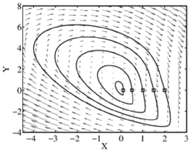
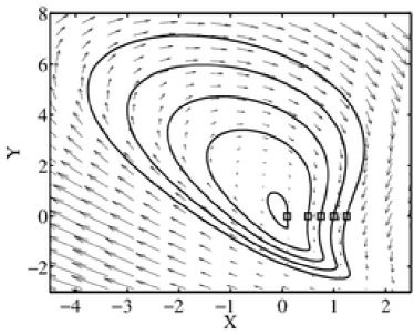
(a) (b)

Figure 1: CMTs (solid lines) in (a), the $(R/{[Q^{\prime}_{s}]_{2}}^{3/2})$–$(Q/[Q^{\prime}_{s}]_{2})$ plane; (b), the $(R/{Q^{\prime}_{s}}^{3/2})$–$(Q/{Q^{\prime}_{s}})$ plane. The trajectories are integrated from the initial conditions $(R/[Q^{\prime}_{s}]_{2}^{3/2},Q/[Q^{\prime}_{s}]_{2})=(0.1,0),(0.5,0),(1,0),(1.5,0)$ and $(2,0)$, and $(R/{Q^{\prime}_{s}}^{3/2},Q/{Q^{\prime}_{s}})=(0.1,0),(0.5,0),(0.75,0),(1,0),(1.25,0)$. The initial positions are marked by $\scriptstyle\Box$. The arrows represent the vector fields, (a), $(V_{R}/[Q^{\prime}_{s}]_{2}^{2},V_{Q}/[Q^{\prime}_{s}]_{2}^{3/2})h/u_{\tau}$ from equation (3); (b), $(v_{R},v_{Q})h/u_{\tau}$ from (5).

2.3 Data filtering

The three velocities components $u_{i}(\boldsymbol{x})$, with $\boldsymbol{x}=(x_{1},x_{2},x_{3})$, are low-pass filtered with a Gaussian cut-off,

$$\widetilde{u}_{i}(\boldsymbol{x})=\iiint_{V}a\cdot u_{i}(\boldsymbol{x}-\boldsymbol{x}^{\prime})\exp\left(-\left(\frac{\pi x_{1}^{\prime}}{\Delta_{1}}\right)^{2}-\left(\frac{\pi x_{2}^{\prime}}{\Delta_{2}}\right)^{2}-\left(\frac{\pi x_{3}^{\prime}}{\Delta_{3}}\right)^{2}\right)\mathrm{d}x_{1}^{\prime}\mathrm{d}x_{2}^{\prime}\mathrm{d}x_{3}^{\prime},$$ (7)

for $i=1,2$ and $3$, where $\Delta_{1}$, $\Delta_{2}$ and $\Delta_{3}$ are the filter widths in the streamwise, wall-normal and spanwise directions, respectively, $V$ is the channel domain extended as explained below and $a$ a constant such that the integral of the kernel over $V$ is one. The Gaussian filter is directly applied in the two homogeneous directions. However, that is not possible in $x_{2}$ due to the wall. To overcome this difficulty, the filtering operation is extended in the wall-normal direction by reflecting the filter at the walls as if they were a mirror (that is equivalent to copy the velocity field above the top wall and below the bottom one reversing the $x_{2}$ direction) and inverting the sign of $u_{2}$ (see figure 2). In this way, the filtered velocity remains incompressible. To assess the effect of this particular approach, all the results in the present manuscript were recomputed using the alternative filter described in Appendix B, and the differences turned out to be negligible. Another possible option was to simply filter in the wall-normal direction and not only in $x_{1}$ and $x_{3}$ as usually done for convenience in the literature. However, we will show that the two approaches are not equivalent.

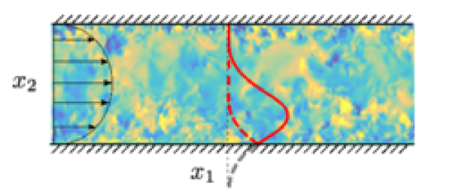
Figure 2: Sketch of the filter kernel reflected at the wall. The red solid line represents the Gaussian kernel in the $x_{2}$ direction, the gray dashed line its extension out of the domain and the red dashed one its reflection. The colormap is the wall-normal velocity.

The aspect ratios of the three filter widths are chosen to be elongated in the streamwise and spanwise directions, and such that $\Delta_{1}/\Delta_{2}=3$ and $\Delta_{3}/\Delta_{2}=1.5$, which is motivated by the characteristic geometrical shape of eddies attached to the wall in the logarithmic layer reported by previous works (Lozano-Durán et al., 2012; del Álamo et al., 2006; Jiménez, 2012). A homogeneous aspect ratio, $\Delta_{1}/\Delta_{2}=1$ and $\Delta_{3}/\Delta_{2}=1$, was also tested and qualitatively similar results were obtained as discussed in Appendix A.

In the present work, we only filter the velocities but quantities computed from them will be also denoted by $\widetilde{(\cdot)}$. For instance, $\widetilde{Q}$ is the second invariant of the velocity gradient tensor computed from the filtered velocities. Consistently, the material derivative of the quantity $\widetilde{\psi}$ is computed with respect to the filtered velocity $\mathrm{D}\widetilde{\psi}/\mathrm{D}t=\partial\widetilde{\psi}/\partial t+\widetilde{u_{i}}\partial\widetilde{\psi}/\partial x_{i}$.

Case	$\Delta_{1}/h$	$\Delta_{2}/h$	$\Delta_{3}/h$	Lines and symbols	Color
F0 (unfiltered)	black	-	-
F0.10	0.30	0.10	0.15	$-$$\circ$$-$	magenta
F0.20	0.60	0.20	0.30	$-$$\scriptstyle\triangle$$-$	blue
F0.25	0.75	0.25	0.38	$-$$\scriptstyle\Box$$-$	green
F0.30	0.90	0.30	0.45	$-\times-$	red
F0.40	1.20	0.40	0.60	$-\Diamond-$	yellow

Table 2: Summary of cases. The parameters $\Delta_{1}$, $\Delta_{2}$ and $\Delta_{3}$ are the filter widths in the streamwise, wall-normal and spanwise direction, respectively. The velocity field is filtered according to (7). The filtered cases are denoted by F$\gamma$, where $\gamma$ is the wall-normal filter width, $\Delta_{2}/h$. The symbols and colors in the last two columns are used to denote the different cases in the figures unless otherwise specified.

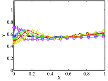
(a) (b)

Figure 3: (a) Root-mean-squared streamwise velocity fluctuations, normalized with $u_{\tau}$ from the unfiltered case, as a function of the wall-normal distance, $x_{2}$. (b) Root-mean-squared third invariant, $R^{\prime}(x_{2})$, normalized by $Q^{\prime 3/2}(x_{2})$. Symbols and colors are as in table 2.

Based on the filtered velocity, the invariants and their total derivatives are then calculated as described in §2.2. The results are computed for six filter widths summarized in Table 2. The first case corresponds to unfiltered data, and the rest are denoted by F$\gamma$, where $\gamma$ is the wall-normal filter width, $\Delta_{2}/h=0.1,0.2,0.25,0.3$ and $0.4$. Note that the largest filter width is $\Delta_{1}=1.2h$, which is still far from the streamwise length of the computational domain $L_{1}\approx 6.3h$. The effects of the size of the box on the results presented in this manuscript turned out to be negligible compared to those in larger domains, and are briefly discussed in Appendix A.

As previously mentioned, we compute the invariants of the filtered velocity components which are the ones usually used in the literature and perhaps also more useful for comparison with experimental data, which sometimes suffer from limited spatial resolution and measure coarse-grained velocity fields. Note that $u_{1}$ can be expressed as $u_{1}=\widetilde{u}_{1}+u_{1,r}$, where $u_{1,r}$ is the residual and $\widetilde{u}_{1}$ the filtered velocity. This filtering approach has the clear physical meaning of removing those scales smaller than the filter width. However, there is a shortcoming when non-linear terms are considered (e.g. kinetic energy or the invariants $R$ and $Q$) and mixed terms of the type $\widetilde{u}_{1}u_{1,r}$ appear. This poses a problem in the sense that it is not clear whether they should be added to the filtered quantity or to the residuals. Hence, another possibility for obtaining filtered invariants would be to filter $R$ and $Q$ directly. This approach does not suffer from the ambiguity above because there are no mixed terms, but the physical meaning is less clear, e.g. filtered $k$ is not the kinetic energy of a well defined velocity field. For that reason, this approach is not used in the present work.

The root-mean-square of the streamwise velocity fluctuations for the filtered and unfiltered cases is shown in figure 3(a). Similar trends are observed in the wall-normal and spanwise velocity fluctuations (not shown). The invariants are normalized as shown in (4), and for the filtered data, the resulting $\widetilde{Q}^{\prime}(x_{2})$ of each case is used. The vector field, $\boldsymbol{v}$, from (5) is normalized with the time scale $h/u_{\tau}$. Figure 3(b) shows that this normalization provides a very good collapse of $R^{\prime}$, at least far from the wall.

3 Results

3.1 R and Q joint distributions

In this section, we compare the invariants computed from the filtered and unfiltered velocity fields. The results are presented in figure 4(a), which shows the joint probability density functions (p.d.f.s) of $R$ and $Q$ for all the cases in table 2. For comparison, figure 4(b) includes the conditionally averaged velocity $\boldsymbol{v}$ from (5) for case F0.25. Similar vector fields are obtained for the other cases although they are omitted for the sake of brevity. Consistent with earlier findings (Borue & Orszag, 1998; van der Bos et al., 2002; Lüthi et al., 2007), the iso-probability lines maintain a tear-drop shape for the filtered cases, and the strain production dominates over enstrophy production in strain-dominated regions also in the inertial scales. This result differs from the more symmetrical p.d.f.s obtained for the coarse-grained velocity reported in previous works (Chertkov et al., 1999; Naso & Pumir, 2005; Naso et al., 2007; Pumir & Naso, 2010) and computed through a stochastic tetrad model based on the evolution of four tracer points. Nevertheless, Lüthi et al. (2007) showed that the latter results are aliased and that the tear-drop shape is recovered when the velocity derivatives are computed using a larger number of tracers.

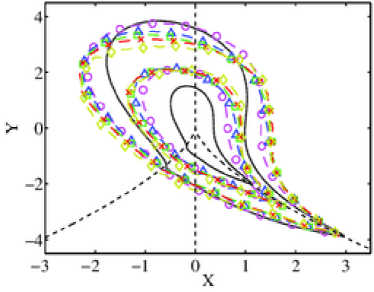
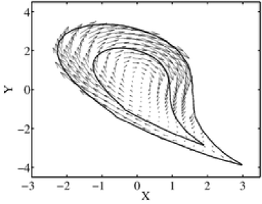
(a) (b)

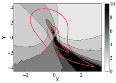
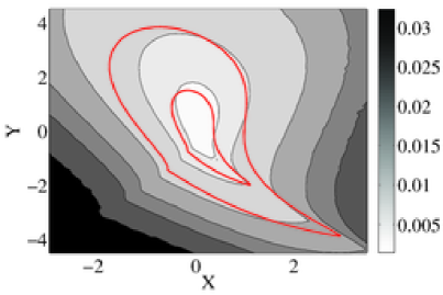
(c) (d)

Figure 4: (a) Joint probability density functions of $R$ and $Q$. The iso-probability contours contain 90% and 98% of the data (that is, 90% and 98% of the data points are enclosed by each contour respectively), corresponding to $1.5\times 10^{-4}$ and $3.3\times 10^{-6}$ of the maximum of the p.d.f.s. The dashed lines are $R=0$ and $D=0$. Symbols and color are as in table 2. (b) Vector field $\boldsymbol{v}$ for F0.25. The solid lines contain 90% and 98% of the data. (c) Ratio of the magnitude of the conditionally averaged velocity deviation $\boldsymbol{v}_{std}$ and the mean $\boldsymbol{v}$, conditioned on the $R$–$Q$ plane. Results for the unfiltered case. Although the colorbar ranges from 0 to 10, values up to 100 are attained close to the Vieillefosse tail. (d) Magnitude of the conditionally averaged velocity deviation $\boldsymbol{v}_{std}h/u_{\tau}$. Red solid lines in (c) and (d) contain 90% and 98% of the data for the probability density function of $R$ and $Q$.

The five filtered cases collapse well except for some small differences for large values of $Q$. However, they differ from the unfiltered case along the horizontal axis where the iso-contours of the filtered ones tend to broaden, meaning that for a given level of $Q$, the invariant $R$ is stronger than in the unfiltered case.

The fairly good overlap between the filtered cases also indicates that the normalization with $\widetilde{Q}^{\prime}$ is appropriate. Without the normalization, the values for the filtered cases are strongly reduced by several orders of magnitude with respect to the unfiltered case (not shown), since strong and intermittent events are mostly caused by the small scale structure of turbulence (Batchelor & Townsend, 1949; Jiménez, 2000). The good collapse for the filtered cases suggests that the dynamics on the $R$–$Q$ plane are self-similar in the inertial range, although it will be shown in section 3.3 that this is not the case for their enstrophy and strain components.

Note that the vectors in figure 4(b) are statistical representations of the conditional dynamics of the flow, and only represent the evolution of individual particles when their standard deviation is small with respect to the mean. Otherwise, they should be considered as small residuals of a more complex underlying evolution. This does not mean that they are irrelevant to the flow. They represent evolutionary trends, in the same sense as the bulk flow of a low-Mach-number fluid is a small residue of the much faster random motion of its molecules. To shed some light on that, figure 4(c) shows the ratio of the magnitudes of $\boldsymbol{v}$ and of the deviation vector

$$\boldsymbol{v}_{std}=\left\langle\left(\left[\frac{\mathrm{D}}{\mathrm{D}t}\left(\frac{R}{{Q^{\prime}}^{3/2}}\right)\right]_{std},\left[\frac{\mathrm{D}}{\mathrm{D}t}\left(\frac{Q}{{Q^{\prime}}}\right)\right]_{std}\right)\right\rangle_{R/{Q^{\prime}}^{3/2},Q/{Q^{\prime}}},$$ (8)

where the subindex $std$ denotes standard deviation at each $R/{Q^{\prime}}^{3/2},Q/{Q^{\prime}}$ point. The average velocity field is relevant at those points where $|\boldsymbol{v}_{std}|$ is much smaller than $|\boldsymbol{v}|$, with $|\cdot|$ the $L^{2}$-norm. In most of the $R$–$Q$ plane, $|\boldsymbol{v}_{std}|/|\boldsymbol{v}|$=3–5, meaning that $\boldsymbol{v}$ is not highly representative of the trajectories of individual fluid particles but rather a weak trend of their motion. This is particularly pronounced along the Vieillefosse tail, where the ratio achieves values up to $100$. Similar results were reported by Lüthi et al. (2009). This effect is caused by the small values attained by the mean rather than by the standard deviation as seen in figure 4(d), which shows $|\boldsymbol{v}_{std}|$ without dividing by the mean. Figure 4(c) corresponds to the unfiltered case, and qualitatively similar values are obtained for the filtered ones (see example in Appendix D).

3.2 Conditional mean trajectories

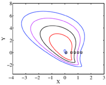
(a) (b)

(c) (d)

(e) (f)

Figure 5: CMTs in the $R$–$Q$ plane computed as shown in (5). The initial $R$ and $Q$ positions (marked by $\scriptstyle\Box$) are the same for all of the cases, $(R/{Q^{\prime}_{s}}^{3/2},Q/{Q^{\prime}_{s}})=(0.1,0),(0.5,0),(0.75,0),(1,0),(1.25,0)$. (a), case F0; (b), case F0.1; (c), case F0.2; (d), case F0.25; (e), case F0.3; (f), case F0.4.

The CMTs are shown in figure 5. It is important to remark that accurate calculation of CMTs is numerically challenging, and the inwards spiraling observed in many works is spurious. We have shown in section 2.2 that our numerics are good enough to recover closed CMTs when the full domain is considered. Results in figure 5 are physical and not the byproduct of numerical artifacts.

Lozano-Durán et al. (2015) showed that unfiltered CMTs, scaled as in (5), describe closed trajectories when the whole channel domain is considered (see figure 1), and the same result is found to be valid here for the filtered cases (not shown). When the p.d.f. is computed in a subdomain defined by two wall-parallel planes, as it is done for the logarithmic region in this paper, the trajectories need not to be closed any more. In that case, the equation for the conservation of probability of $J=J(R/Q^{\prime 3/2},Q/Q^{\prime})$ for a stationary state is

$$\boldsymbol{\nabla}_{R,Q}\cdot\left(J\boldsymbol{v}\right)=\psi_{t}+\psi_{b},$$ (9)

where

$$\boldsymbol{\nabla}_{R,Q}=\left(\frac{\partial}{\partial R/Q^{\prime 3/2}},\frac{\partial}{\partial Q/Q^{\prime}}\right),$$ (10)

$\boldsymbol{v}$ is as defined in (5). $\psi_{b}$ and $\psi_{t}$ are the probability fluxes at the bottom plane ($x_{2}^{+}=100$) and at the top plane ($x_{2}/h=0.4$)

$$\psi_{b} = \alpha V_{b}J_{b},$$ (11)

$$\psi_{t} = -\alpha V_{t}J_{t},$$ (12)

where $V_{b}$, $V_{t}$, $J_{b}$ and $J_{t}$ are functions of $(R/Q^{\prime 3/2},Q/Q^{\prime})$. $V_{b}$ and $V_{t}$ are the conditional wall-normal velocities on the $R/Q^{\prime 3/2}$–$Q/Q^{\prime}$ plane at $x_{2}=x_{b}$ and $x_{2}=x_{t}$, respectively, and $J_{b}$ and $J_{t}$ the probability density functions at those same heights. $\alpha$ is a scale-factor equal to $1/(x_{t}-x_{b})$. For $x_{b}$ and $x_{t}$ equal to the bottom and top walls, fluxes (11) and (12) become zero and equation (9) is equivalent to the stationary Fokker-Planck equation used in previous works (van der Bos et al., 2002; Chevillard et al., 2008, 2011). Some guidelines for deriving equation (9) are provided in Appendix C.

Figure 5(a) shows that, for the unfiltered case, the CMTs describe clockwise cycles around the origin in almost closed trajectories, consistently with the results from Lozano-Durán et al. (2015), who observed a probability flux of strong $R$–$Q$ leaving the buffer layer and entering the outer zone, but which canceled when both boundaries were considered.

For the filtered cases (figures 5b to 5f), the CMTs spiral outwards. Intuitively, this is caused by the unbalanced of $R$ and $Q$ associated with the fluid leaving and entering the subdomain through the boundaries, and can be better understood by studying the fluxes $\psi_{b}$ and $\psi_{t}$ shown in figures 6(a) and (b) for case F0.25. At the bottom boundary, incoming fluxes are located at the first ($R>0$ and $Q>0$) and third ($R<0$ and $Q<0$) quadrant, whereas at the top one they concentrate at the centre of the $Q$–$R$ plane. The resulting net effect $\psi_{b}+\psi_{t}$ (figure 6c) is dominated by incoming flux of weak events into the logarithmic layer, and a secondary outflow of stronger events distributed in the second and fourth quadrants. Qualitatively similar results are obtained for other filter widths (not shown).

In conclusion, the outward spiraling is mainly due to weaker normalized $R$ and $Q$ transported from the outer region into the logarithmic layer, where they are amplified. Results from the remaining cases (not shown) reveal that the increasing spiraling with wider filter widths is caused by the influx from the lower boundary being damped by the filter, while fluxes across the upper boundary remain similar. If the effect of the viscous terms is considered negligible for the filtered cases, the outward spiraling of inertial CMTs may be attributed to the combined effect of self-amplification, pressure and interscale transfer. Note that the outward spiraling also implies that the residual CMTs, i.e., those which added to the filtered cases result in the unfiltered one, must spiral inwards in order to recover the almost closed CMTs in figure 5(a). This may be caused by viscous and/or interscale transfer effects (among others), and a term-by-term analysis of the dynamic equations of $\widetilde{R}$ and $\widetilde{Q}$ (and of the residual counterparts) would be necessary to address this question in detail. This will be tackled in future studies.

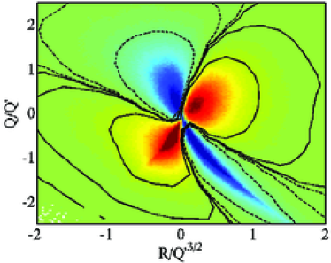
(a) (b)

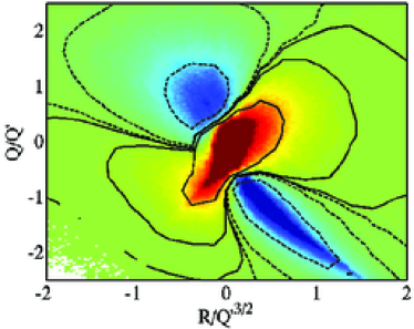
(c)

Figure 6: Probability fluxes from equation (11) and (12) at plane (a), $x_{2}^{+}=100$ ($\psi_{b}$); (b) $x_{2}/h=0.4$ ($\psi_{t}$); and (c), net flux through both boundaries ($\psi_{b}+\psi_{t}$). Positive values are represented by hot colors and solid contours. Negative values are cold colors and dashed lines. Contours are $\pm 10^{-1}$, $\pm 10^{-2}$ and $\pm 10^{-3}$ of the maximum. Data for F0.25.

3.3 Strain and enstrophy components

Despite the similarities found for the joint distributions of $R$ and $Q$ in the previous section, we show below that decomposing the invariants in their strain and enstrophy components leads to quite pronounced differences. Following Ooi et al. (1999), $Q$ and $R$ are decomposed as

$$Q_{s} = -\frac{1}{2}s_{ij}s_{ij},\quad Q_{\omega}=\frac{1}{4}\omega_{i}\omega_{i},$$ (13)

$$R_{s} = -\frac{1}{3}s_{ij}s_{jk}s_{ki},\quad R_{\omega}=-\frac{1}{4}\omega_{i}\omega_{j}s_{ij},$$ (14)

so that $Q=Q_{s}+Q_{\omega}$ and $R=R_{s}+R_{\omega}$. Note that this decomposition differs from that in Soria et al. (1994); Blackburn et al. (1996) and Davidson (2004) who considered the invariants of the rate-of-strain, $s_{ij}$, and rate-of-rotation, $\Omega_{ij}$, tensors. In those cases, $Q_{s}$ and $R_{s}$ coincide with the second and third invariants of $s_{ij}$, and so does $Q_{\omega}$ with the second invariant of $\Omega_{ij}$. However, the third invariant of $\Omega_{ij}$ is zero and $R_{\omega}$ is not.

Relations (13) and (14) show that $Q_{\omega}$ is proportional to the enstrophy density whose intense values tend to concentrate in tube-like structures (Jiménez et al., 1993). $Q_{s}$ is proportional to the strain, which is proportional to the local rate of viscous dissipation of kinetic energy, $\varepsilon=-4\nu Q_{s}$, with high values organized in sheets or ribbons (Moisy & Jiménez, 2004). The meaning of $R_{s}$ and $R_{\omega}$ is closely connected to the evolution equations for the strain and enstrophy densities, that for the filtered cases are (see Ooi et al. (1999) for the original equations for the unfiltered case)

$$\frac{D}{Dt}\left(\frac{\widetilde{\omega}_{i}\widetilde{\omega}_{i}}{2}\right) = \widetilde{\omega}_{i}\widetilde{\omega}_{j}\widetilde{s}_{ij}+\nu\widetilde{\omega}_{i}\frac{\partial^{2}\widetilde{\omega}_{i}}{\partial x_{k}\partial x_{k}}+\epsilon_{ilm}\widetilde{\omega}_{i}\frac{\partial^{2}\tau_{mk}}{\partial x_{l}\partial x_{k}},$$ (15)

$$\frac{D}{Dt}\left(\frac{\widetilde{s}_{ij}\widetilde{s}_{ij}}{2}\right) = -\widetilde{s}_{ik}\widetilde{s}_{kj}\widetilde{s}_{ij}-\frac{1}{4}\widetilde{\omega}_{i}\widetilde{\omega}_{j}\widetilde{s}_{ij}-\widetilde{s}_{ij}\frac{\partial^{2}\widetilde{p}}{\partial x_{i}\partial x_{j}}+\nu\widetilde{s}_{ij}\frac{\partial^{2}\widetilde{s}_{ij}}{\partial x_{k}\partial x_{k}}+\widetilde{s}_{ij}\frac{\partial B_{ijk}}{\partial x_{k}},$$ (16)

where $\tau_{mk}=\widetilde{u}_{m}\widetilde{u}_{k}-\widetilde{u_{m}u_{k}}$ and $B_{ijk}=1/2(\partial\tau_{ik}/\partial x_{j}+\partial\tau_{jk}/\partial x_{i})$ are responsible for the interscale transfer of strain and enstrophy. The corresponding relations for the unfiltered case are recovered by taking $\tau_{ik}=0$. Relations (15) and (16) show that $R_{s}$ and $R_{\omega}$ are proportional to the strain self-amplification and enstrophy production, respectively. We will use $Q^{\prime}_{s}(x_{2})$ to non-dimensionalize quantities related to the strain (such as $Q_{s}$ and $R_{s}$) and $Q^{\prime}_{\omega}(x_{2})$ for those related to the enstrophy (such as $Q_{\omega}$ and $R_{\omega}$). The material derivatives are computed for the normalized quantities as in (5).

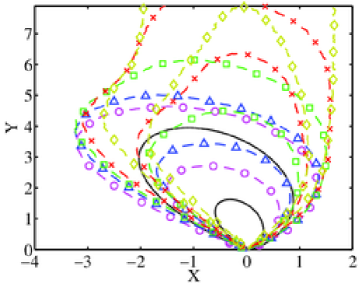
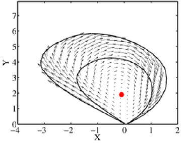
(a) (b)

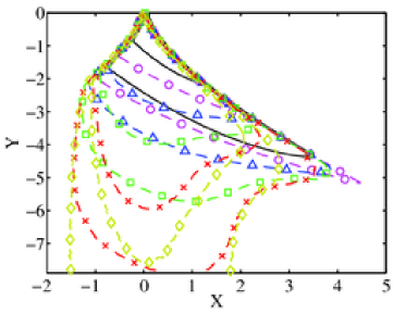
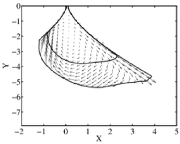
(c) (d)

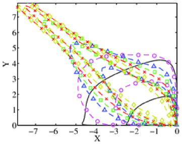
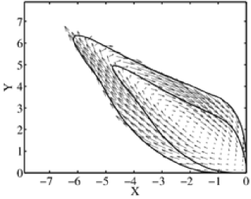
(e) (f)

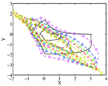
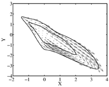
(g) (h)

Figure 7: Joint probability density functions of (a) and (b), $R_{\omega}$–$Q_{\omega}$; (c) and (d), $R_{s}$–$Q_{s}$; (e) and (f), $Q_{s}$–$Q_{\omega}$; (g) and (h), $R_{s}$–$R_{\omega}$. The left column includes the conditionally averaged velocity $\boldsymbol{v}$ for case F0. Symbols and colors as in table 2. The right column includes the joint p.d.f. and $\boldsymbol{v}$ for F0.25. The contours contain 90% and 98% of the data. The red dot in (b) is $\boldsymbol{v}=\boldsymbol{0}$. See text for details about the normalization.

The joint p.d.f.s for several combinations of (13) and (14) are plotted in figure 7. Figures 7(a,c,e,g) show the iso-probability contours for all of the cases in table 2, and the corresponding conditionally averaged velocity for the unfiltered case. For comparison, figures 7(b,d,f,h) show the contours and velocities for F0.25. In all of them, the corresponding conditional velocity $\boldsymbol{v}$ reveals a cyclical behavior of the CMTs that is consistent with previous literature, e.g. Ooi et al. (1999); Lüthi et al. (2009). Although not shown for the distributions in figure 7, $|\boldsymbol{v}_{std}|/|\boldsymbol{v}|$ attains values similar to those reported above in the $R$–$Q$ plane (see examples in Appendix D).

One of the most remarkable results is the lack of collapse of the p.d.f.s for the different filter widths. The distributions in the $Q_{\omega}$–$R_{\omega}$ and $Q_{s}$–$R_{s}$ planes lose their skewed shape, at least partially compared to the unfiltered case, and become more symmetric, specially for $\Delta_{2}\geq 0.3h$. On the contrary, the enstrophy and strain densities become increasingly anti-correlated as the filter width grows, and follow the relation, $Q_{s}\approx-Q_{\omega}$. The same result applies to the enstrophy production and strain self-amplification distributions which exhibit a strong anti-correlation, $R_{s}\approx-R_{\omega}$, although in this case the trend saturates above $\Delta_{2}=0.2h$. Note that $Q_{s}=-Q_{\omega}$, i.e. $Q=0$, represents a degenerate flow topology (Chong et al., 1990) that can be associated with pure shear, and that $R_{s}=-R_{\omega}$ implies a linear relation between enstrophy production and strain self-amplification.

The results above reveal that a lot of information is hidden in the $R$–$Q$ plane, and that decomposing the invariants in their strain and enstrophy contributions offers a more comprehensive view to study the dynamics of the flow. The resulting dynamics in the $R$–$Q$ plane are obtained by adding the quantities $Q_{s}+Q_{\omega}$ and $R_{s}+R_{\omega}$ which have similar magnitude but opposite signs most of time, making it difficult to predict the final shape of the $R$–$Q$ iso-contour in figure 4(a) from those in figure 7(a). It is still intriguing how the tear-drop shape persists at different scales despite the changes undergone by the strain and enstrophy components of $R$ and $Q$.

The lack of collapse in the previous results may be explained taking into account the increasing contribution of $\partial\widetilde{u}_{1}/\partial x_{2}$ with the filter width. We can write the relations for $\widetilde{Q}_{s}$, $\widetilde{Q}_{\omega}$, $\widetilde{R}_{s}$ and $\widetilde{R}_{\omega}$ in the limiting case in which the wall-normal derivative of $\widetilde{u}_{1}$ is the most important gradient,

$$\widetilde{Q}^{S}_{s} = -\frac{1}{4}\left(\frac{\partial\widetilde{u}_{1}}{\partial x_{2}}\right)^{2},\quad\widetilde{Q}^{S}_{\omega}=\frac{1}{4}\left(\frac{\partial\widetilde{u}_{1}}{\partial x_{2}}\right)^{2},$$ (17)

$$\widetilde{R}^{S}_{s} = \frac{1}{4}\frac{\partial\widetilde{u}_{3}}{\partial x_{3}}\left(\frac{\partial\widetilde{u}_{1}}{\partial x_{2}}\right)^{2},\quad\widetilde{R}^{S}_{\omega}=-\frac{1}{4}\frac{\partial\widetilde{u}_{3}}{\partial x_{3}}\left(\frac{\partial\widetilde{u}_{1}}{\partial x_{2}}\right)^{2}.$$ (18)

The superscript $S$ is used to distinguish them from the regular definitions in (13) and (14). Relations (17) and (18) show that $\widetilde{Q}^{S}_{s}=-\widetilde{Q}^{S}_{\omega}$ and $\widetilde{R}^{S}_{s}=-\widetilde{R}^{S}_{\omega}$, which is consistent with the trends observed in figures 7(e,g). In order to test whether the decomposed invariants are dominated by the contribution of $\partial\widetilde{u}_{1}/\partial x_{2}$ as the filter width increases, figure 8(a) shows the ratios of the standard deviations, $Q^{\prime S}_{s}/Q^{\prime}_{s}$, $Q^{\prime S}_{\omega}/Q^{\prime}_{\omega}$, $R^{\prime S}_{s}/R^{\prime}_{s}$ and $R^{\prime S}_{\omega}/R^{\prime}_{\omega}$ averaged in $x_{2}$ along the log-layer, denoted by $\overline{(\cdot)}$, and as a function of the filter width. The results suggest that the dynamics of the eddies are progressively controlled by $\partial\widetilde{u}_{1}/\partial x_{2}$ as their scale increases. Note that $\partial\widetilde{u}_{1}/\partial x_{2}$ is the instantaneous gradient but is related to the mean shear, $S$, by averaging in the homogeneous directions and in time. This is in agreement with Corrsin’s argument (Corrsin, 1958) whereby the dynamics of the eddies with sizes comparable or larger than the Corrsin scale, $l_{C}=(\varepsilon/S^{3})^{1/2}$, are dominated by the effect of the mean shear. It is also consistent with $l_{C}$ being on average $\approx 0.08h$ in the range considered for the logarithmic layer, which is well below the filter widths used (see table 2). The key role of $S$ in the dynamics of wall-attached eddies in the logarithmic layer have also been highlighted in previous works (Jiménez, 2013; Lozano-Durán & Jiménez, 2014b). At this point, it is interesting to add that the trends shown above are much weaker if the filter is only performed in the homogeneous but not in $x_{2}$, and the reader is referred to Appendix E for more details and some examples.

Another conclusion from (17) and (18) is that the distributions $\widetilde{Q}_{s}$–$\widetilde{R}_{s}$ and $\widetilde{Q}_{\omega}$–$\widetilde{R}_{\omega}$ should become mirror images of each other as the filter width increases, since their variables may be interchanged as $\widetilde{Q}_{s}\rightarrow-\widetilde{Q}_{\omega}$ and $\widetilde{R}_{s}\rightarrow-\widetilde{R}_{\omega}$. This is clearly visible in figures 7(a,c) for F0.4. Figure 8(b) shows that the skewness of $\widetilde{R}_{s}$ and $\widetilde{R}_{\omega}$ decreases, and justifies the increasingly symmetrical shape of the $\widetilde{Q}_{s}$–$\widetilde{R}_{s}$ and $\widetilde{Q}_{\omega}$–$\widetilde{R}_{\omega}$ distributions with the $\Delta_{2}$ (figures 7(a) and (c) respectively). Exact zero average enstrophy production is not expected for any filter width, since averaging (15) yields to

$$\langle\widetilde{\omega}_{i}\widetilde{\omega}_{j}\widetilde{s}_{ij}\rangle=-\langle\nu\widetilde{\omega}_{i}\frac{\partial^{2}\widetilde{\omega}_{i}}{\partial x_{k}\partial x_{k}}\rangle-\langle\epsilon_{jil}\widetilde{\omega}_{l}\frac{\partial^{2}\tau_{ik}}{\partial x_{k}\partial x_{j}}\rangle,$$ (19)

where $\langle\cdot\rangle$ denotes ensemble average. Assuming that the viscous effects are negligible at the inertial scales, (19) implies that the average filtered enstrophy production is not zero but balanced by the interscale transfer of enstrophy density.

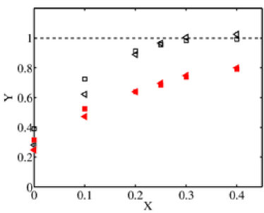
(a) (b)

Figure 8: (a) Ratios of the standard deviation of the terms defined by (17) and (18), and those in (13) and (14), averaged along the log-layer and as a function of the filter width, $\Delta_{2}$. $\scriptstyle\Box$, $\overline{Q^{\prime S}_{s}/Q^{\prime}_{s}}$; $\triangleleft$, $\overline{Q^{\prime S}_{\omega}/Q^{\prime}_{\omega}}$; $\blacksquare$, $\overline{R^{\prime S}_{s}/R^{\prime}_{s}}$; $\blacktriangleleft$, $\overline{R^{\prime S}_{\omega}/R^{\prime}_{\omega}}$. (b) Skewness of the probability density functions of $\scriptstyle\Box$, $R_{s}/{Q^{\prime}_{s}}^{3/2}$; $\scriptstyle\triangle$, $R_{\omega}/{Q^{\prime}_{\omega}}^{3/2}$, as a function of the wall-normal filter width, $\Delta_{2}$. The skewnesses for the unfiltered cases are omitted and roughly equal to $\pm 40$.

Case	$\Delta_{1}/h$	$\Delta_{2}/h$	$\Delta_{3}/h$	Lines and symbols	Color
S0 (unfiltered)	black	-	-
S0.10	0.30	0.10	0.15	$-$$\circ$$-$	magenta
S0.20	0.60	0.20	0.30	$-$$\scriptstyle\triangle$$-$	blue
S0.25	0.75	0.25	0.38	$-$$\scriptstyle\Box$$-$	green
S0.30	0.90	0.30	0.45	$-*-$	yellow
S0.40	1.20	0.40	0.60	$-\Diamond-$	black

Table 3: Summary of cases computed for the velocity fluctuations. The parameters $\Delta_{1}$, $\Delta_{2}$ and $\Delta_{3}$ are the filter widths in streamwise, wall-normal and spanwise directions, respectively. The fluctuating velocity field is filtered according to (7). The cases are denoted by S$\gamma$, where $\gamma$ is the wall-normal filter width, $\Delta_{2}/h$. The symbols and colors in the last columns are used to denote the different cases in the figures.

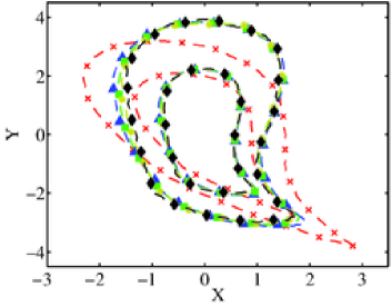
(a) (b)

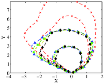
(c) (d)

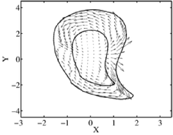
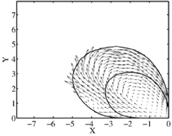
(e) (f)

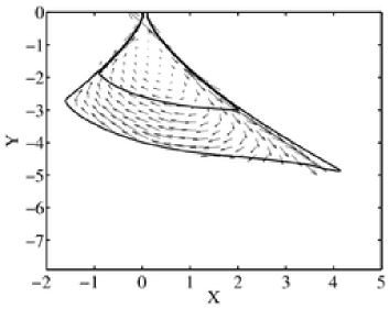
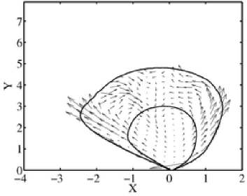
(g) (h)

Figure 9: Results computed for the velocity fluctuations. Joint probability density functions of (a), $R$–$Q$; (b), $Q_{s}$–$Q_{\omega}$; (c), $R_{s}$–$Q_{s}$; (d), $R_{\omega}$–$Q_{\omega}$. The iso-probability contours contain 90% and 98% of the data. Symbols and colors are as in table 3. For comparison, one more case is included: $\times$, case F0.3. (e), (f), (g), and (h), conditionally averaged velocity field computed as in (5) in the planes (e), $R$–$Q$; (f), $Q_{s}$–$Q_{\omega}$; (g), $R_{s}$–$Q_{s}$; (h), $R_{\omega}$–$Q_{\omega}$. The contours are 90% and 98% of the data of the corresponding p.d.f.. Results for case S0.25. See text for details about the normalization.

The direct effect of the mean shear in the previous results may be removed by computing the invariants of the velocity fluctuations instead of those of the total velocity. Hence, six more cases were computed using the fluctuating velocities, and their parameters are summarized in table 3. The new cases are denoted by S$\gamma$, where $\gamma$ is the wall-normal filter width, $\Delta_{2}/h$, with the same aspect ratios $\Delta_{1}/\Delta_{2}$ and $\Delta_{3}/\Delta_{2}$ as in F$\gamma$. Although not shown, the differences in the probability distributions in figure 7 computed with and without the mean shear are insignificant for the unfiltered case, meaning that the small scales are barely affected by $S$.

The results for S$\gamma$ are shown in figure 9. One noteworthy difference is the change in the joint p.d.f.s of $\widetilde{R}$ and $\widetilde{Q}$, which become more symmetric and lose a large portion of the Vieillefosse tail (figure 9a). The strong correlation between $\widetilde{Q}_{s}$ and $\widetilde{Q}_{\omega}$ is also lost (figure 9b) and the good collapse of the iso-probability contours reinforces the conclusion that the mean shear is responsible for the trends observed in figures 7. The distribution of $\widetilde{R}_{s}$–$\widetilde{R}_{\omega}$ behaves in a similar manner (not shown). The joint p.d.f.s of $\widetilde{Q}_{s}$–$\widetilde{R}_{s}$ and $\widetilde{Q}_{\omega}$–$\widetilde{R}_{\omega}$ become more symmetric too (figures 9c,d) and, contrary to the results observed for cases F$\gamma$, the contours collapse quite well for $\Delta_{2}>0.1h$. Case S0.1 lies in between S0 and S0.2, probably because it is an intermediate stage between the small and inertial scales, and was omitted from figure 9 for the sake of clarity.

Interestingly, the conditionally averaged velocities for S$\gamma$, computed from $\mathrm{D}/\mathrm{D}t$ based on the fluctuating filtered velocity, do not always rotate around one center as in F$\gamma$ (see figure 7). As an example, figures 9(e-h) contain the conditional velocity $\boldsymbol{v}$ for S0.25, and show that the CMTs in the $R$–$Q$ and $R_{\omega}$–$Q_{\omega}$ planes may be classified into two families according to their clockwise/counter-clockwise rotation. It is remarkable that the trajectories in the upper quadrant of the $R$–$Q$ plane now cycle counter-clockwise, in contrast to the result for the invariants of the total velocity gradient showed in figures 4(c)-(d). The difference comes mostly from the behavior of $R_{\omega}$ and $Q_{\omega}$, since $R_{s}$ and $Q_{s}$ remain similar to those observed in F$\gamma$ (cf. figures 7 and 9). The fluctuating $R$–$Q$ plane may be explained noting that intense contraction of vorticity ($R_{\omega}>0$) is now associated with increasing $Q_{\omega}$ (figure 9h), which is responsible for the counter-clockwise part in the first quadrant of figure 9(e). Also, the strongest $Q_{\omega}$ at negative $R_{\omega}$ (vortex stretching) is associated with decreasing $Q_{\omega}$, which explains the counter clockwise part of the second quadrant in figure 9(e). This very interesting behavior comes from the increase of fluctuating enstrophy ($Q_{\omega}$) in the presence of contraction of vorticity ($R_{\omega}>0$), in contrast to the usual decrease observed for the total velocity. It also implies that $R_{\omega}$ is not the dominant term for the budget of $Q_{\omega}$ (nor $Q$) in those regions, and that the interactions between mean and fluctuating gradients at the inertial scales or the interscale transfer are presumably responsible for these trends. Double cycles similar to those shown in figures 9(e) and (h) for S0.25 appear in the remaining filtered cases too (not shown).

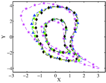
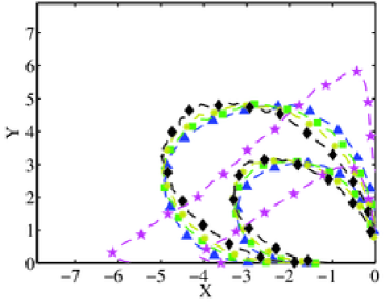
(a) (b)

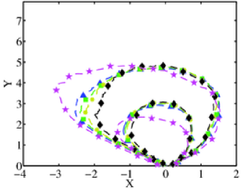
(c) (d)

Figure 10: Results computed for the velocity fluctuations. Joint probability density functions of (a), $R$–$Q$; (b), $Q_{s}$–$Q_{\omega}$; (c), $R_{s}$–$Q_{s}$; (d), $R_{\omega}$–$Q_{\omega}$. The iso-probability contours contain 90% and 98% of the data. Symbols and colors are as in table 3. For comparison, one more case is included, $\bigstar$, isotropic turbulence from JHU turbulence database (Li et al., 2008) filtered with $\Delta_{1}=\Delta_{2}=\Delta_{3}=90\eta$. See text for details about the normalization.

Another interesting question is whether the results for the velocity fluctuations presented above resemble those of isotropic turbulence (HIT). The idea is tested in figures 10(a-d) and turns out not to be the case. The data used is HIT from JHU turbulence database (Li et al., 2008) filtered using (7) with $\Delta_{1}=\Delta_{2}=\Delta_{3}=90\eta$, which is comparable to the filter widths from table 3, where $\Delta_{2}=0.3h\approx 90\eta$. Borue & Orszag (1998) reported distributions consistent with ours from their analysis of HIT using a top-hat filter. The distributions for HIT are more skewed than those for the fluctuations in the channel, specially in the $R$–$Q$ and $Q_{s}$–$R_{s}$ maps. The enstrophy/enstrophy-production p.d.f. for HIT is the only one close to the results obtained for cases S$\gamma$. However, the trends in the $Q_{s}$–$Q_{\omega}$ plane are opposite, and the CMTs from HIT resemble the clockwise cycling of figure 7 rather than the ones observed in figures 9(e) and (h). These results suggest that considering only fluctuating velocities removes the direct effect of the shear on the dynamics but there still remains the indirect effect, which is expected since the mean shear and the fluctuations are coupled by the non-linear dynamics of the Navier–Stokes equations.

3.4 Orbital periods

The CMTs are useful to compute orbital periods, i.e., the time $\tau$ elapsed to complete one full revolution around the stagnation point, $\boldsymbol{v}=\boldsymbol{0}$. This can be done for all the distributions in figure 7, and the results will be shown to be of the same order throughout this section. We focus on the periods in the $Q_{\omega}$–$R_{\omega}$ plane and some examples are discussed for other cases. Figure 11(a) shows the values of $\tau$ as a function of the initial distance to the stagnation point, $r_{0}$ (see figure 7b). Many initial conditions randomly distributed in each plane ($Q_{\omega}$–$R_{\omega}$, $R$–$Q$, etc) were used to compute $\tau$, and its average value is shown in figure 11(a).

The periods collapse reasonable well for all the filter widths when normalized by $\overline{\widetilde{Q}^{\prime}}^{1/2}$ (where the bar represents average along the logarithmic layer) and do not vary much with $r_{0}$, i.e., weak and strong events show similar characteristic time-scales. This is the consequence of the larger velocities sampled by the CMTs as $r_{0}$ increases, which compensates for the longer paths traveled, leading to $\tau\approx$ constant.

For the unfiltered case, $\tau$ decreases $~{}30$% by the time $r_{0}$ has tripled, but it remains always above the filtered cases. The dependence of $\tau$ with $r_{0}$ suggest that weak small-scale events take longer time to complete one dynamic cycle, although the underlying physical meaning is unclear. On average, $\tau\overline{Q^{\prime}}^{1/2}\approx 17$ for the unfiltered case, and $\tau\overline{\widetilde{Q}^{\prime}}^{1/2}\approx 10$ for the filtered ones. Results of the same order but slightly larger are obtained in the $Q_{s}$–$R_{s}$ plane, and one example is included in figure 11(a).

A Kolmogorov-scale normalization, $\tau_{\eta}\sim\overline{Q^{\prime}}^{-1/2}$, where $\tau_{\eta}$ is the Kolmogorov time-scale, is the natural choice for the unfiltered case since $\tau_{\eta}$ is the typical decorrelation time-scale during Lagrangian evolution (Meneveau, 2011). The fact that such a normalization works with $\widetilde{Q}^{\prime}$ for the filtered cases suggests that the dominating eddies in the filtered flow are those with characteristic size $\Delta_{2}$ and lifetimes proportional to their local eddy-turnover time $\overline{\widetilde{Q}^{\prime}}^{-1/2}$.

Figure 11(a) also includes the orbital periods in the $R$–$Q$ plane for case F0.2 and the trend is similar to those computed for other joint distributions. However, our experience shows that the conditionally averaged velocity on the $R$–$Q$ plane changes direction very fast close to the Vieillefosse tail, specially for large filter widths, which poses some numerical issues and makes the CMTs to follow wrong paths. For instance, it was not possible to complete a single orbit for case F0.4 for large $r_{0}$ (figure 5d). The $Q_{\omega}$–$R_{\omega}$ and $Q_{s}$–$R_{s}$ planes are more reliable than the $R$–$Q$ space to compute periods for large filter widths.

The last period computed corresponds to the CMTs from case S0.25 in the $R$–$Q$ plane restricted to $Q>0$ (see figure 9e). The results are included in figure 11(a) and remain within the scatter of previous orbital times. Many other periods can be computed and show different degrees of agreement with those shown before. These are not discussed here since we do not pretend to perform an exhaustive analysis of all the possibilities, but just to remark that they are of the same order.

(a) (b)

Figure 11: (a) Orbital periods of the CMTs, $\tau$, as a function of the distance of their initial condition to the stagnation point of $\boldsymbol{v}$ in the corresponding plane, $r_{0}$. $\blacksquare$, periods computed in the $R$–$Q$ plane for case F0.2; $\blacktriangledown$, periods computed in the $Q_{s}$–$R_{s}$ plane for case F0.2; *, periods computed in the $R$–$Q$ plane for CMTs in the regions $Q>0$ and case S0.25. The rest of the symbols are as in table 2 and correspond to periods extracted from the $Q_{\omega}$–$R_{\omega}$ plane and filter widths $\Delta_{2}=0,0.1,0.2,0.25,0.3$ and $0.4$. (b) Orbital periods of the CMTs in the $Q_{\omega}$–$R_{\omega}$ averaged in $r_{0}$ as a function of the wall-normal filter width, $\Delta_{2}$. The dashed line is $\tau u_{\tau}/h=8\Delta_{2}/h+0.08$.

The value $\tau\overline{\widetilde{Q}^{\prime}}^{1/2}\approx 10$ extracted from figure 11(a) for cases F$\gamma$ implies that the absolute orbital period increases with $\Delta_{2}$, since the magnitude of $\overline{Q^{\prime}}^{1/2}$ decreases with the filter width. Figure 11(b) shows that the relation between orbital periods and filter widths follows approximately the linear trend, $\tau u_{\tau}/h\approx 8\Delta_{2}/h+0.08$, when the time is normalized by the eddy-turnover time, $h/u_{\tau}$. The first and last points, $\Delta_{2}=0$ and $\Delta_{2}=0.4$, were excluded from the previous fitting, the former for being dominated by the viscous effects, and the latter for exceeding or being at the edge of the usual range considered for the logarithmic layer (Marusic et al., 2013). The dependence of $\overline{\widetilde{Q}^{\prime}}^{1/2}$ with $\Delta_{2}$ can be estimated analytically for a known velocity gradient spectrum and, for the range of filter widths considered here, turns out to be almost linear, which explains the trend in figure 11(b). The constant factor based on the filter width and friction velocity, $\Delta_{2}/u_{\tau}$, is a suitable normalization factor for the orbital period.

To close this section we compare our periods with those in the literature. The orbital periods discussed above for the unfiltered case, $\tau\overline{Q^{\prime}}^{1/2}\approx 17$, correspond to $\tau^{+}=280$ and $\tau/\tau_{\eta}=26$ in wall and Kolmogorov units, respectively, with $\tau_{\eta}=\overline{(\nu/\varepsilon)^{1/2}}$. The value obtained by Atkinson et al. (2012) in a turbulent boundary layer flow at a comparable Reynolds number is $\tau^{+}=658$, which exceeds ours, although in their case the periods are computed for the logarithmic and wake region. Elsinga & Marusic (2010) reported a smaller value, $\tau^{+}=470$, which is still larger than ours, although they used experimental data filtered over $50$ wall units in each direction. For isotropic turbulence, Lüthi et al. (2009), Martín et al. (1998) and Ooi et al. (1999) obtained $\tau/\tau_{\eta}\approx 40$ and $\tau/\tau_{\eta}\approx 30$, respectively, which are not so far from the value of $26$ obtained here. Nevertheless, some differences are expected since we compute the Lagrangian time derivative of the normalized invariants, as in (5), and not of the invariants themselves, as it is the case of previous works. It is difficult to find in the literature orbital periods for the filtered invariants, although values of the same order to those shown in figure 11(b) were obtained for the bursting periods, $T_{b}$, of minimal log-layer channels by Flores & Jiménez (2010), $T_{b}u_{\tau}/h\approx 6x_{2}/h$, if we take $\Delta_{2}=x_{2}$. However, it is not simple to establish a link between orbital and bursting periods, and it is unclear whether they are related or not. A linear relation between lifetime and scale has also been observed in previous works (del Álamo et al., 2006; Lozano-Durán & Jiménez, 2014b; LeHew et al., 2013), and is explained in the context of self-similar log-layer eddies with lifetimes proportional to their size. Lozano-Durán & Jiménez (2014b) found $Tu_{\tau}/h\approx\Delta_{2}/h$, with $T$ the lifetimes of wall-attached eddies, and $\Delta_{2}$ their size, that will be considered equivalent to the filter width. However, these lifetimes are much shorter than the orbital periods reported here, $\tau u_{\tau}/h\approx 8\Delta_{2}/h+0.08$. This discrepancy may be related to the ratio $|\boldsymbol{v}_{std}|/|\boldsymbol{v}|$ shown in figure 4(b). The average $|\boldsymbol{v}_{std}|/|\boldsymbol{v}|$ along a CMT is $6$–$12$ for all filter widths, and its inverse value can be interpreted as the fraction of time the fluid particles travel in the ‘correct’ direction to complete a cycle instead of drifting in other directions. This may responsible for the factor of 8 between orbital periods and lifetimes of individual eddies mentioned above.

3.5 Alignment of the vorticity and the rate-of-strain tensor

In order to gain a better insight into the dynamics at different scales, we analyze the alignment of the vorticity vector, $\boldsymbol{\omega}$, with the eigenvectors of the rate-of-strain tensor, $\boldsymbol{\lambda_{1}}$, $\boldsymbol{\lambda_{2}}$, and $\boldsymbol{\lambda_{3}}$, whose associated eigenvalues are $\lambda_{1}>\lambda_{2}>\lambda_{3}$ (note that in this case the subindex refers to the sorting of the eigenvalues, in contrast to the convection used for other quantities, $s_{ij}$, $u_{i}$,… where the index denotes the spatial direction $x_{i}$). This alignment is of interest since the enstrophy production may be expressed as (Betchov, 1956)

$$\omega_{i}\omega_{j}s_{ij}=\omega^{2}\left(p_{1}+p_{2}+p_{3}\right),$$ (20)

where $p_{i}=\lambda_{i}\cos^{2}(\boldsymbol{\omega},\boldsymbol{\lambda_{i}})$ and $\omega$ is the $L^{2}$-norm of $\boldsymbol{\omega}$. An equivalent expression applies to the filtered cases.

Since the trace of $s_{ij}$ must be zero owing to incompressibility, it is satisfied that $\lambda_{1}>0$ and $\lambda_{3}<0$. The former eigenvalue represents stretching in the direction of $\boldsymbol{\lambda_{1}}$, whereas the latter is a contraction of vorticity along $\boldsymbol{\lambda_{3}}$. The second eigenvalue, $\lambda_{2}$, takes both positive and negative values and it is well-known that, for the small scales, $\boldsymbol{\omega}$ aligns preferentially with $\boldsymbol{\lambda_{2}}$ in isotropic turbulence (Ashurst et al., 1987), free shear flows (Mullin & Dahm, 2006) and turbulent channels (Blackburn et al., 1996). Similar results hold for the filtered cases as shown in figure 12(a). However, the alignment of $\boldsymbol{\omega}$ and $\boldsymbol{\lambda_{2}}$ intensifies for larger scales and, as a result, the angles of $\boldsymbol{\lambda_{1}}$ and $\boldsymbol{\lambda_{3}}$ with $\boldsymbol{\omega}$ tend to zero, i.e., perpendicular to $\boldsymbol{\omega}$ (not shown).

(a) (b)

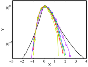
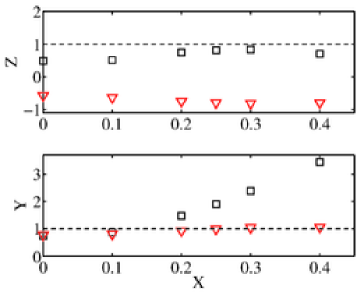
(c) (d)

Figure 12: Results computed for the total velocities. (a) Probability density functions of the cosine of the angle of the vorticity, $\boldsymbol{\omega}$, and the second eigenvector of the rate-of-strain tensor, $\boldsymbol{\lambda_{2}}$. (b) and (c) are the probability density functions of the eigenvalues of the rate-of-strain tensor, (b), $\lambda_{1}$ and $\lambda_{3}$; (c), $\lambda_{2}$. For (a), (b) and (c) the symbols and colors are as in table 2. (d) Relative contributions to the enstrophy production of $p_{1}=\lambda_{1}\cos^{2}(\boldsymbol{\omega},\boldsymbol{\lambda_{1}})$, $p_{2}=\lambda_{2}\cos^{2}(\boldsymbol{\omega},\boldsymbol{\lambda_{2}})$ and $p_{3}=\lambda_{3}\cos^{2}(\boldsymbol{\omega},\boldsymbol{\lambda_{3}})$ as a function of the wall-normal filter width, $\Delta_{2}$. The top panel shows the ratio of the means, $\scriptstyle\Box$, $\langle p_{2}\rangle/\langle p_{1}\rangle$; $\scriptstyle\triangle$, $\langle p_{3}\rangle/\langle p_{1}\rangle$. The bottom panel shows the ratio of the standard deviations, $\scriptstyle\Box$, $p^{\prime}_{2}/p^{\prime}_{1}$; $\scriptscriptstyle\bigtriangledown$, $p^{\prime}_{3}/p^{\prime}_{1}$.

Figures 12(b,c) show the p.d.f.s of $\lambda_{i}$ scaled by the corresponding ${Q^{\prime}_{s}}^{1/2}$ of each case. The distribution for the unfiltered $\lambda_{2}$ is skewed towards positive values as already reported in previous works (Ashurst et al., 1987; Vincent & Meneguzzi, 1991; Blackburn et al., 1996). The p.d.f.s of $\lambda_{1}$ do not collapse for the different filter widths, nor they do for $\lambda_{2}$ and $\lambda_{3}$, respectively, although the distributions become more symmetric as $\Delta_{2}$ increases, consistent with the results for the skewness of $R_{\omega}$ in figure 8(b).

The preferential alignment of $\boldsymbol{\omega}$ with $\boldsymbol{\lambda_{2}}$ is predicted by angular momentum conservation in the Restricted Euler Model (Cantwell, 1992), and was explained from a kinematic point of view in Jiménez (1992). Such an alignment, or at least part of it, may also be expected in the context of eddies controlled by the mean shear as proposed in section 3.3. In fact, in the very simple scenario in which $\partial u_{1}/\partial x_{2}$ is the most important term, the flow behaves like a pure shear, and $\boldsymbol{\omega}$ and $\boldsymbol{\lambda_{2}}$ align (Tennekes & Lumley, 1972). In this case, the associated $\lambda_{2}$ tends to zero, which is a consequence of the over-simplifications made and could be solved by retaining higher order terms.

The preferential alignment of $\boldsymbol{\omega}$ with $\boldsymbol{\lambda_{2}}$ does not imply that most of the contribution to the enstrophy production is due to $\omega^{2}p_{2}$ (Tsinober et al., 1997). Figure 12(d) shows the relative importance of $p_{1}$, $p_{2}$ and $p_{3}$ in terms of its mean $\langle\cdot\rangle$ (top panel), and its standard deviation $(\cdot)^{\prime}$ (bottom panel), for different filter widths. For the unfiltered case, the contributions of $\langle p_{2}\rangle$ and $\langle p_{3}\rangle$ to the mean enstrophy production/destruction are, in magnitude, roughly one half of the contribution of $\langle p_{1}\rangle$, which turns out to be the most important term (Vincent & Meneguzzi, 1994; Tsinober, 1998). When filtering, the ratios $\langle p_{2}\rangle/\langle p_{1}\rangle$ and $\langle p_{3}\rangle/\langle p_{1}\rangle$ approach to $\pm 1$, respectively. This implies that the small-scale vortices are mostly dominated by vortex stretching, but large-scale vorticity is equally influenced by the three terms from (20). From a geometric point of view, the results above suggest that the tube-like structures are favored at the small scales but that sheet-like objects dominate at larger ones as in the geometrical analysis of turbulent structures in Moisy & Jiménez (2004). The scale-dependence of the ratios is even more pronounced for the standard deviations of $p_{i}$, and $p^{\prime}_{2}/p^{\prime}_{1}$ increases steadily, attaining values up to three times those of $p^{\prime}_{3}/p^{\prime}_{1}$.

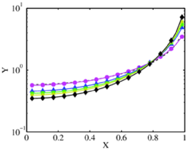
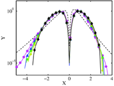
(a) (b)

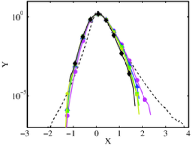
(c) (d)

Figure 13: Same as figure 13 but for the fluctuating velocities (cases S$\gamma$ table 3). For (a), (b) and (c) the symbols and colors are as in table 3.

The results above suggest that the dynamics of the flow differ at different scales. However, it was noticed in section 3.3 that this may be caused by the effect of the mean shear. For that reason, the calculations were repeated for cases S$\gamma$, where only the velocity fluctuations are considered, and the results are shown in figure 13. The fluctuating vorticity also aligns predominantly with the second eigenvector of the fluctuating rate-of-strain tensor (figure 13a), implying that the alignment shown in figure 12(a) is not entirely caused by the effect of the mean shear, and the distributions of the three eigenvalues become more symmetric, specially for $\Delta_{2}>0.1h$ (figures 13b,c). The main difference compared to the results computed for the total velocities is the improved collapse of the p.d.f.s for both the alignments and eigenvalues. Figure 13(d) is equivalent to figure 12(d), but the ratios remain roughly constant and independent from the filter width, suggesting that vortices defined through the fluctuating velocities are better candidates than the total vorticity to study the multiscale dynamics of the flow. This scale-independent behavior also suggest that these large-scale vortices are geometrically self-similar as opposed to those described above for the total velocities, although that should be tested in more detail with a geometrical analysis of the structures that is out of the scope of the present paper. From the results above, we can conclude that once the direct effect of the mean shear is removed, the multiscale dynamics of the enstrophy production become roughly self-similar, consistent with the results shown before for the joint distributions of $Q_{s}$, $Q_{\omega}$, $R_{s}$ and $R_{\omega}$ associated with the fluctuating velocity.

3.6 The energy cascade in terms of vortex stretching

In the previous section we have studied the alignment of the vorticity and the eigenvectors of the rate-of-strain tensor at the same scale. Here we analyze the alignment of vorticity and strain at different ones, i.e., the vorticity associated with the filtered velocity at scale $\Delta^{\omega}$, whose quantities will be denoted by $\widetilde{(\cdot)}$, and the rate-of-strain associated with the filtered velocity at a scale $\Delta^{s}$, represented by $\widehat{(\cdot)}$. The study is motivated by the classical energy cascade in terms of vortex stretching, where the strain at a given scale stretches the vortices at a smaller one and induces higher velocities by the conservation of angular momentum. This scenario provides a mechanism for the interscale energy transfer required by the energy cascade, but is presumably in contradiction with previous studies (Ashurst et al., 1987; She et al., 1991; Vincent & Meneguzzi, 1994) and with section 3.5, where the vorticity aligns most probably with the intermediate strain eigenvector. This may be caused by the fact that $\boldsymbol{\omega}$ and $s_{ij}$ are both studied at the same scale, and it has been noted before that the alignment of vorticity with the intermediate strain eigenvector decreases when the local strain induced by the vortices is eliminated (Jiménez, 1992; Hamlington et al., 2008). This suggests that such an alignment could change for vorticity fields and strain tensors calculated each at a different scale.

(a) (b)

Figure 14: Probability density functions of the cosine of the angle of the vorticity, $\widetilde{\boldsymbol{\omega}}$, filtered with $\Delta^{\omega}_{2}$, and the eigenvectors of the rate-of-strain tensor,   , $\widehat{\boldsymbol{\lambda}}_{1}$;            , $\widehat{\boldsymbol{\lambda}}_{2}$;                , $\widehat{\boldsymbol{\lambda}}_{3}$, filtered with $\Delta^{s}_{2}$. (a) $\Delta^{\omega}_{2}=0.05h$ and $\Delta^{s}_{2}=0.55h$, (b) $\Delta^{\omega}_{2}=0.55h$ and $\Delta^{s}_{2}=0.05h$. Results computed for the total velocity.

The previous idea was tested in Leung et al. (2012) for isotropic turbulence and a few scales. Here we extend the study to the logarithmic layer of a turbulent channel and a wider range of scales. We will denote the streamwise, wall-normal and spanwise filter widths by $\Delta^{j}_{1}$, $\Delta^{j}_{2}$ and $\Delta^{j}_{3}$ with $j=\omega,s$, and ratios as described in §2.3. The interest of this analysis is further motivated by figure 14(a), which shows that the roles of $\widehat{\boldsymbol{\lambda}}_{1}$ and $\widehat{\boldsymbol{\lambda}}_{2}$ change completely for $\Delta^{\omega}_{2}=0.05h$ and $\Delta^{s}_{2}=0.55h$ compared to those reported for the vorticity and strain at the same scale. In this particular case, the smaller-scale vorticity aligns predominantly with the most extensional eigenvector and is stretched by the larger-scale strain. On the other hand, figure 14(b) shows that the p.d.f.s of $\cos(\widetilde{\boldsymbol{\omega}},\widehat{\boldsymbol{\lambda}}_{i})$ follow a uniform distribution with no preferential alignment when computed for $\Delta^{\omega}_{2}=0.55h$ and $\Delta^{s}_{2}=0.05h$, i.e., large-scale vorticity versus smaller-scale strain.

It is difficult to infer the causal relation between scales from instantaneous flow fields without a more detailed time-resolved information of the flow. However, it is reasonable to suppose that, on average, the causality is from larger scales to smaller ones, since the characteristic times of the former are longer than those of the latter. Thus, for $\Delta^{s}_{2}>\Delta^{\omega}_{2}$, we will assume that the vorticity is stretched/compressed by the larger-scale strain, and vice versa for $\Delta^{\omega}_{2}>\Delta^{s}_{2}$.

To perform a more systematic analysis of the dominant alignment of $\widetilde{\boldsymbol{\omega}}$ and $\widehat{\boldsymbol{\lambda}}_{i}$, we expand the number of filters previously used in order to sample the scale-space in more detail. The new wall-normal filter widths range from $\Delta^{j}_{2}=0.05h$ to $\Delta^{j}_{2}=0.55h$ in increments of $0.05h$ with $j=\omega,s$, and all the possible combinations of $(\Delta^{\omega}_{2},\Delta^{s}_{2})$ are considered, which yields a total number of 121 cases. Alignments are measured by the ratio of probabilities of $|\cos(\widetilde{\boldsymbol{\omega}},\widehat{\boldsymbol{\lambda}}_{i})|>0.9$, with $i=1,2,3$, for each $(\Delta^{\omega}_{2},\Delta^{s}_{2})$ pair,

$$r_{i}(\Delta^{\omega}_{2},\Delta^{s}_{2})=\frac{P(|\cos(\widetilde{\boldsymbol{\omega}},\widehat{\boldsymbol{\lambda}}_{i})|>0.9)}{P(|\cos(\widetilde{\boldsymbol{\omega}},\widehat{\boldsymbol{\lambda}}_{2})|>0.9)},\ i=1,3$$ (21)

where $P$ stands for probability, and $|\cos(\widetilde{\boldsymbol{\omega}},\widehat{\boldsymbol{\lambda}}_{2})|>0.9$ is used as a reference value. $\cos(\alpha)=0.9$ corresponds to an angle close to $\pi/7$ radians or $25^{\circ}$, and $r_{i}>1$ implies a dominant alignment of $\widetilde{\boldsymbol{\omega}}$ and $\widehat{\boldsymbol{\lambda}}_{i}$. The discussion below is valid for values equal to 0.7 and 0.8 are used instead of 0.9.

Results for $r_{i}$ are shown in figure 15, where low values of the $r_{1}$ and $r_{3}$ appear along the diagonal $\Delta^{s}_{2}=\Delta^{\omega}_{2}$, in agreement with the dominant alignment of $\widetilde{\boldsymbol{\boldsymbol{\omega}}}$ and $\widetilde{\boldsymbol{\boldsymbol{\lambda}}}_{2}$ discussed in §3.5. For $\Delta^{s}_{2}>\Delta^{\omega}_{2}$ (upper diagonal), the alignment of $\widetilde{\boldsymbol{\omega}}$ and $\widehat{\boldsymbol{\lambda}}_{1}$ increases with the distance to the diagonal, consistent with the energy cascade framework described above. This is specially the case for low values of $\Delta^{\omega}_{2}$, around $0.05-0.10h$, and $\Delta^{s}_{2}>0.2h$, where $r_{1}\approx 1.6$. For $\Delta^{s}_{2}<\Delta^{\omega}_{2}$ (lower diagonal), the alignment of $\boldsymbol{\omega}$ and $\widehat{\boldsymbol{\lambda}}_{3}$ increases (compression of the flow field by large-scale vorticity) although the effect is weaker than the one observed in the upper diagonal for $r_{1}$. It is important to remark that the probability distributions flatten in this region, as shown in figure 14(b), and the peaks at $|\cos(\widetilde{\boldsymbol{\omega}},\widehat{\boldsymbol{\lambda}}_{i})|=1$ are less pronounced than those found in the upper diagonal. It was checked that the kurtosis coefficients of the p.d.f.s in the lower diagonal are closer to the theoretical value of a perfectly flat distribution than those in the upper part (not shown). This suggests that the alignment of $\widetilde{\boldsymbol{\omega}}$ and $\widehat{\boldsymbol{\lambda}}_{3}$ are less relevant than the one of $\widetilde{\boldsymbol{\omega}}$ and $\widehat{\boldsymbol{\lambda}}_{1}$ for $\Delta^{s}_{2}>\Delta^{\omega}_{2}$.

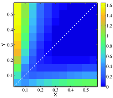
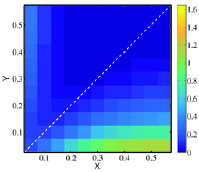
(a) (b)

Figure 15: (a) Ratio of the probability of $|\cos(\widetilde{\boldsymbol{\omega}},\widehat{\boldsymbol{\lambda}}_{1})|>0.9$ and $|\cos(\widetilde{\boldsymbol{\omega}},\widehat{\boldsymbol{\lambda}}_{2})|>0.9$ as a function of the vorticity and strain wall-normal filter widths, $\Delta^{\omega}_{2}$ and $\Delta^{s}_{2}$, respectively. Values equal to one imply equal probability of finding $|\cos(\widetilde{\boldsymbol{\omega}},\widehat{\boldsymbol{\lambda}}_{1})|>0.9$ and $|\cos(\widetilde{\boldsymbol{\omega}},\widehat{\boldsymbol{\lambda}}_{2})|>0.9$. (b) Same as (a) but for the ratio of the probability of $|\cos(\widetilde{\boldsymbol{\omega}},\widehat{\boldsymbol{\lambda}}_{3})|>0.9$ and $|\cos(\widetilde{\boldsymbol{\omega}},\widehat{\boldsymbol{\lambda}}_{2})|>0.9$. The dashed line is $\Delta^{\omega}_{2}=\Delta^{s}_{2}$. Results computed for the total velocity.

The $\widetilde{\boldsymbol{\omega}}$–$\widehat{\boldsymbol{\lambda}}_{i}$ alignments presented in figure 15 are of little value if its contribution to the enstrophy production of $\widetilde{\omega}^{2}$ is negligible. The dynamical equation for the average enstrophy from (19) can be re-written neglecting the viscous term as

$$\langle\widetilde{\omega}_{i}\widetilde{\omega}_{j}\widetilde{s}_{ij}\rangle=\langle\widetilde{\omega}_{i}\widetilde{\omega}_{j}\widehat{s}_{ij}\rangle+\langle\widetilde{\omega}_{i}\widetilde{\omega}_{j}s^{r}_{ij}\rangle\approx-\langle\epsilon_{jil}\widetilde{\omega}_{l}\frac{\partial^{2}\tau_{ik}}{\partial x_{k}\partial x_{j}}\rangle,$$ (22)

where $\widetilde{s}_{ij}$ has been decomposed into its contribution from scale $\Delta^{s}_{2}$ and a residual term such that $\widetilde{s}_{ij}=\widehat{s}_{ij}+s^{r}_{ij}$. Relation (22) shows that the enstrophy production may be expressed as the interaction of $\widetilde{\omega}_{i}$ and $\widehat{s}_{ij}$ plus a residual, and that the sum of both is balanced by the interscale transfer term on the right-hand-side. Note that the $\widetilde{\boldsymbol{\omega}}$–$\widehat{\boldsymbol{\lambda}}_{i}$ alignment calculated above is directly related to the enstrophy production $\widetilde{\omega}_{i}\widetilde{\omega}_{j}\widehat{s}_{ij}$. The importance of this term is quantified in figure 16(a), which shows the ratio

$$r^{p}(\Delta^{\omega}_{2},\Delta^{s}_{2})=\frac{\langle\widetilde{\omega}_{i}\widetilde{\omega}_{j}\widehat{s}_{ij}\rangle}{\sqrt{\langle\widetilde{\omega}_{i}\widetilde{\omega}_{j}\widehat{s}_{ij}\rangle^{2}+\langle\widetilde{\omega}_{i}\widetilde{\omega}_{j}s^{r}_{ij}\rangle^{2}}},$$ (23)

for all the possible combinations of filter widths. By definition, the diagonal elements must be $1$ since $s^{r}_{ij}=0$ and $\langle\widetilde{\omega}_{i}\widetilde{\omega}_{j}\widehat{s}_{ij}\rangle>0$. Interestingly, the data reveal that $r^{p}$ reaches values close to 1 for $\Delta^{s}_{2}>\Delta^{\omega}_{2}$, and the contribution of $\langle\widetilde{\omega}_{i}\widetilde{\omega}_{j}\widehat{s}_{ij}\rangle$ is large enough to support the idea of a non-negligible role of vortex stretching in the energy cascade. Surprisingly, $r^{p}$ is also large in magnitude but negative for scales in the far lower part. The term (22) appears in the dynamic equation for $\widehat{s}_{ij}\widehat{s}_{ij}$ acting as a source but with opposite sign. This suggests an interesting connection between large-scale vorticity and small-scale strain, closing the self-sustained cascade process. However, we have shown above that in that case there is no preferential alignment between vorticity and strain eigenframe (figure 14b) and the physical relevance of this result is unclear. A simplified sketch of the different scenarios is shown in figure 17.

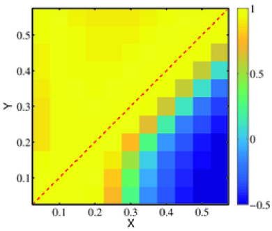
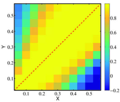
(a) (b)

Figure 16: Ratio of the average enstrophy productions, $r^{p}$, as a function of the wall-normal filter width for the vorticity, $\Delta^{\omega}_{2}$ denoted by $\widetilde{(\cdot)}$ and the strain, $\Delta^{s}_{2}$ denoted by $\widehat{(\cdot)}$. Results computed from (a), total velocity; (b), fluctuating velocity.

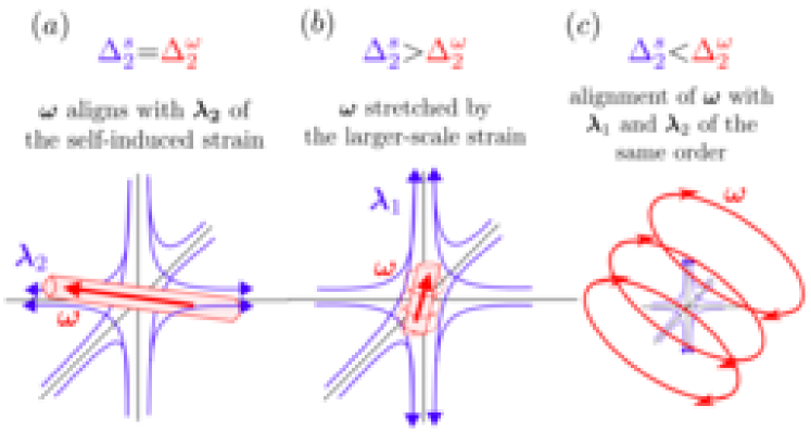
Figure 17: Sketches of the vorticity-strain interaction. (a) At the same scale; (b), strain-scale larger than vorticity-scale; (c), strain-scale smaller than vorticity-scale.

The results shown so far were calculated for the total velocity, and following the structure of previous sections, they were repeated for the fluctuations. Most of the conclusions discussed for the total velocity apply to the fluctuating vorticity and rate-of-strain tensor. The most remarkable difference is found in the ratio $r^{p}$ in figure 16(b). The contribution of $\langle\widetilde{\omega}_{i}\widetilde{\omega}_{j}\widehat{s}_{ij}\rangle$ decays with the distance to the diagonal and is around 20–30% of $\langle\widetilde{\omega}_{i}\widetilde{\omega}_{j}\widetilde{s}_{ij}\rangle$ at those places where the alignment of $\widetilde{\boldsymbol{\omega}}$ and $\widehat{\boldsymbol{\lambda}}_{1}$ is of the same order as the one from $\widetilde{\boldsymbol{\omega}}$ and $\widehat{\boldsymbol{\lambda}}_{2}$ (figure 18a). Figure 18 also shows that $r_{1}$ and $r_{3}$ attain values below those obtained for the total velocity, which may be connected to the counter-clockwise behavior in the $R_{\omega}$–$Q_{\omega}$ plane in figure 9(h) and discussed in §3.3.

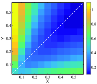
(a) (b)

Figure 18: (a) Ratio of the probability of $|\cos(\widetilde{\boldsymbol{\omega}},\widehat{\boldsymbol{\lambda}}_{1})|>0.9$ and $|\cos(\widetilde{\boldsymbol{\omega}},\widehat{\boldsymbol{\lambda}}_{2})|>0.9$ as a function of the vorticity and strain wall-normal filter widths, $\Delta^{\omega}_{2}$ and $\Delta^{s}_{2}$, respectively. Values equal to one imply equal probability of finding $|\cos(\widetilde{\boldsymbol{\omega}},\widehat{\boldsymbol{\lambda}}_{1})|>0.9$ and $|\cos(\widetilde{\boldsymbol{\omega}},\widehat{\boldsymbol{\lambda}}_{2})|>0.9$. (b) Same as (a) but for the ratio of the probability of $|\cos(\widetilde{\boldsymbol{\omega}},\widehat{\boldsymbol{\lambda}}_{3})|>0.9$ and $|\cos(\widetilde{\boldsymbol{\omega}},\widehat{\boldsymbol{\lambda}}_{2})|>0.9$. The dashed line is $\Delta^{\omega}_{2}=\Delta^{s}_{2}$. Results computed for the fluctuating velocity.

4 Conclusions

We have studied the dynamics of the invariants of the filtered velocity gradient tensor, $R$ and $Q$, in the logarithmic layer of an incompressible turbulent channel flow. The invariants are gradients of the velocities and hence, are dominated by the effect of the small scales. By filtering the velocity field, we have applied the topological and physical tools provided by the invariants to scales in the inertial range.

We have paid special attention to the numerics involved in the computation of the invariants in order to minimize numerical errors as much as possible. The spatial derivatives were computed with spectral methods, and the number of modes expanded by a factor of three in each direction to reduce aliasing problems. The temporal derivatives were computed with fourth-order finite differences using velocity fields contiguous in time. Besides, all the calculations were performed in double precision. More details about the numerical procedure can be found in Lozano-Durán et al. (2015).

In order to compensate for the wall-normal inhomogeneity of the channel, the invariants were scaled by the standard deviation of the second invariant, $Q^{\prime}$, as a function of the distance to the wall, and their material derivatives were consistently computed to obtained closed trajectories when the whole channel domain is considered as in Lozano-Durán et al. (2015).

The effect of filtering on the joint probability density function of $R$ and $Q$, $J(R,Q)$, is found to be rather weak. The tear-drop shape persists for larger scales, consistent with previous findings (Borue & Orszag, 1998; van der Bos et al., 2002; Lüthi et al., 2007), and the most noteworthy change is the widening of $J(R,Q)$ along the $R$ axis for the filtered cases.

The conditional mean trajectories in the normalized $R$–$Q$ plane rotate clockwise for all of the cases. The CMTs describe almost closed trajectories in the unfiltered case when normalized as $R/Q^{\prime 3/2}$ and $Q/Q^{\prime}$. However, they spiral outwards in the filtered cases, and this effect intensifies with the filter width. The probability fluxes show that the previous equilibrium is not achieved at the inertial scales, in the sense that fluid from the outer region with associated weak invariants enters to the logarithmic layer, and is later intensified, that is, CMTs spiral outwards to larger values of the normalized $R$ and $Q$.

Surprisingly, when the calculations were repeated for the invariants of the fluctuating velocity gradient, the CMTs split into two families for $Q<0$ and $Q>0$, with trajectories rotating clockwise and counter-clockwise, respectively. The latter differs from the CMTs of the invariants of the total velocity gradient tensor, and the cause was traced back to the enstrophy/enstrophy-production cycle. It was found that increasing enstrophy was on average associated with contraction of vorticity, and therefore, the upper counter clockwise cycle in the $R$–$Q$ plane can not be a consequence of the enstrophy production (as it is for the total velocity) but the result of the interaction of the fluctuations with the shear or with the interscale transfer. Nevertheless, it was also shown that they are the result of an averaging process where the mean is 3-5 times smaller than the corresponding standard deviation, and the CMTs represent broad trends that may differ quite significantly from the instantaneous behavior of the individual flow particles.

Decomposing the invariants $R$ and $Q$ in their enstrophy ($Q_{\omega}$ and $R_{\omega}$) and strain ($Q_{s}$ and $R_{s}$) components reveals substantial changes compared to those observed in the $R$–$Q$ plane. As the filter width increases, the strain/strain-self-amplification and enstrophy/enstrophy-production distributions become more symmetric. On the contrary, the joint p.d.f.s of $Q_{s}$–$Q_{\omega}$ and $R_{s}$–$R_{\omega}$ become progressively anti-correlated, i.e., $Q_{s}\approx-Q_{\omega}$ and $R_{s}\approx-R_{\omega}$. These results were explained considering that the filter diminishes the effect of the small scales in favor of larger wall-attached eddies, whose dynamics are controlled by the mean shear (Lozano-Durán et al., 2012; del Álamo et al., 2006; Flores & Jiménez, 2010; Jiménez, 2012). Interestingly, when the direct effect of the mean shear is removed by computing the normalized invariants of the fluctuating velocities, all the p.d.f.s collapse for filter widths $\Delta_{2}>0.1h$, suggesting a self-similar multiscale behavior of the fluctuating strain and enstrophy dynamical cycles. Nevertheless, the results obtained for the fluctuating velocities differ from those for isotropic turbulence, which is an indication that some indirect effect of the mean shear remains.

The orbital period $\tau$, i.e., the time employed by the CMTs to complete one full revolution, computed in the $R$–$Q$, $Q_{\omega}$–$R_{\omega}$ and $Q_{s}$–$R_{s}$ planes are all of the same order, which is expected since they represent the same dynamical cycle projected at different planes. Besides, the periods are independent of the initial position of the CMTs, namely weak and strong events have the same time-scale for a given filter width. This was explained by noting that the trajectories associated with weak regions in a certain space have shorter lengths but also slower conditional velocities. As the CMTs move towards stronger events, they travel longer distances but also move faster. These two effects compensate resulting in a roughly constant $\tau$. If we consider that strong and weak events are respectively associated with small and large scales, that is not strictly rigorous but reasonable on average, the previous results may be related to the classical turbulent cascade where the energy is fed into the largest scales and cascades downwards until is ultimately dissipated at the smallest ones. In this scenario, the evolution of the small scales is enslaved by the larger ones, and the orbital periods of the strong small-scale events would simply reflect the effect of the weaker larger ones (Jiménez, 2013; Cardesa et al., 2015).

The orbital periods collapse for all the filter widths when scaled by $\widetilde{Q}^{\prime-1/2}$, that is the natural eddy-turnover time of eddies at scale $\Delta_{2}$. Also, when expressed as a function of the filter width, they follow $\tau u_{\tau}/h\approx 8\Delta_{2}/h+0.08$. A linear relation between lifetimes and scales has already been observed in previous works (del Álamo et al., 2006; LeHew et al., 2013; Lozano-Durán & Jiménez, 2014b) in the context of self-similar eddies in the logarithmic layer with lifetimes proportional to their sizes, and dynamics controlled by the mean shear. The periods obtained here are 8 times larger than the lifetimes of individual eddies reported by Lozano-Durán & Jiménez (2014b) if $\Delta_{2}$ is taken as the characteristic size of the wall-attached motions. This disparity may be related to the large velocity differences between CMTs and instantaneous trajectories mentioned above. In this sense, the orbital periods are the average time required by the fluid particles to undergo all the different topologies, or from a dynamical point of view, to complete one cycle (in the enstrophy/enstrophy-production, strain/strain-self-amplification planes…) progressively.

The angle between the vorticity and the eigenvectors of the rate-of-strain tensor was also studied as a function of the filter width. The results showed that the vorticity, $\boldsymbol{\omega}$, tends to align with the second eigenvector of the rate-of-strain tensor, $\boldsymbol{\lambda_{2}}$, which intensifies as the filter width increases. Despite this, if the enstrophy production is decomposed as the sum of $p_{i}=\lambda_{i}\cos(\boldsymbol{\omega},\boldsymbol{\lambda_{i}})^{2}$ with $i=1,..,3$, most of the contribution to its mean ($\langle\cdot\rangle$) is caused by $\langle p_{1}\rangle$ in the unfiltered case, but $\langle p_{2}\rangle$ and $\langle p_{3}\rangle$ steadily increase and decrease, respectively, until they equal in magnitude the contribution of the first for large filter widths. The changes in the ratio of the standard deviations of $p_{i}$ as a function of the filter width is even more pronounced. Again, this scale-dependent behavior was explained in terms of the mean shear. When the calculations were repeated for the fluctuating velocities, the results became scale-independent. In this case, there is still a preferential alignment of $\boldsymbol{\omega}$ and $\boldsymbol{\lambda_{2}}$, but a similar contribution of $\langle p_{1}\rangle$, $\langle p_{2}\rangle$ and $\langle p_{3}\rangle$ to the mean enstrophy production at all the scales. The previous results reinforce the idea of self-similar dynamics in the inertial range when the direct effect of the mean shear is removed.

Finally, we have investigated the energy cascade in terms of vortex stretching where vortices at a given scale are stretched by the strain at a larger one. We have shown that the preferred alignment of the vorticity and the intermediate eigenvector of the strain decreases when vorticity and strain are each considered at a different scale. In particular, the alignment of lower-scale vorticity and larger-scale strain increases with the scale separation, and reaches values of the same order or larger than those obtained at same scale. Moreover, these interscale interactions between strain and vorticity attain values between $0.5$-$1.6$ of those of the total enstrophy production at the $\boldsymbol{\omega}$ scale. The scenario is qualitatively similar for the fluctuating velocity but with a weaker alignment of $\boldsymbol{\omega}$ and $\boldsymbol{\lambda_{1}}$, and contributions to the total enstrophy production around $0.2$-$0.3$. Although the results support a non-negligible role of the phenomenological energy-cascade model formulated in terms of vortex stretching, the details of such a cascade remain unknown, and time-resolved data at higher Reynolds numbers is required to perform a thorough analysis of the process.

Appendix A Effects of the Reynolds number, computational domain and filter width aspect ratios

The results presented in this paper were also computed for a DNS of a turbulent channel at $Re_{\tau}=550$ with a resolution $\delta_{1}$, $\delta_{2}$ and a numerical domain equal to the ones shown in table 1. The p.d.f.s at $Re_{\tau}=550$ collapse with those at $Re_{\tau}=932$ in the $R$–$Q$ plane as shown in figure 19(a). However, the trends observed in the distributions of the decomposed invariants at $Re_{\tau}=932$ are qualitatively similar but less pronounced at $Re_{\tau}=550$. Figure 19(b) shows the joint p.d.f.s of $Q_{s}$ and $Q_{\omega}$ as an example.

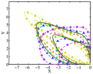
(a) (b)

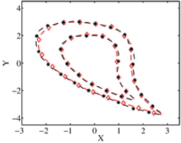
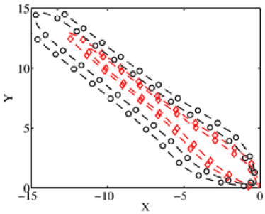
(c) (d)

Figure 19: (a) Joint probability density function of (a), $R$–$Q$ and (b), $Q_{s}$ and $Q_{\omega}$ at $Re_{\tau}=550$. Symbols and colors are as in table 2. The solid line is case F0.2. (c) Joint probability density function of $R$ and $Q$ computed for channels with streamwise and spanwise lengths of $\Diamond$, $L_{1}=2\pi h$ and $L_{3}=\pi h$; *, $L_{1}=8\pi h$ and $L_{3}=3\pi h$. In both cases the data was filtered with $\Delta_{1}=1.2h$, $\Delta_{2}=0.4h$ and $\Delta_{2}=0.6h$. (d) Joint probability density functions of $Q_{s}$ and $Q_{\omega}$ filtered with $\Diamond$, $\Delta_{1}=0.9h$, $\Delta_{2}=0.3h$ and $\Delta_{2}=0.45h$; $\circ$, $\Delta_{1}=\Delta_{2}=\Delta_{2}=0.6h$.

We address next the effect of the computational domain in the results presented above. The dataset were computed in boxes with streamwise and spanwise dimensions of $L_{1}=2\pi h$ and $L_{3}=\pi h$, respectively. Lozano-Durán & Jiménez (2014b) showed that these domains are large enough to correctly capture the dynamics of the logarithmic layer. However, this was done for the unfiltered case and it remains unclear whether it is also valid for filtered fields. The most restrictive case is the one with the larger filter width, i.e., case F0.4 (see table 2). Figure 19(b) compares the iso-probability contours of $R$-$Q$ for case F0.4 with the results obtained from a turbulent channel at the same Reynolds number, filtered with the same filter width but with a much larger computational domain, $L_{1}=8\pi h$ and $L_{3}=3\pi h$. The agreement between the p.d.f.s computed in both domains is almost perfect and suggests that the results in the previous sections are independent of the size of the domain.

The ratio of the filter widths $\Delta_{1},\Delta_{2}$ and $\Delta_{3}$ was chosen $\Delta_{1}/\Delta_{2}=3$, $\Delta_{3}/\Delta_{2}=1.5$ to match the size of the eddies educed by Lozano-Durán & Jiménez (2014b). This has a caveat, because the effect of the filter is smaller in the wall-normal derivatives than in the others. It was tested that modifying the aspect ratio of the filter widths does not alter the dominant role of $\partial u_{1}/\partial x_{2}$ and qualitatively similar results to those presented in the paper persist. Figure 19(d) shows one example with a homogeneous filter $\Delta_{1}=\Delta_{2}=\Delta_{3}=0.6h$ to illustrate that the strong correlation between $Q_{s}$ and $Q_{\omega}$ remains.

Appendix B Alternative filter

To assess the effect of (7), all the results were recomputed using the filter

$$\widetilde{u}_{i}(\boldsymbol{x})=\iiint_{Vr}u_{i}(\boldsymbol{x}-\boldsymbol{x}^{\prime})f(x_{2})\exp\left(-\left(\frac{\pi x_{1}^{\prime}}{\Delta_{1}}\right)^{2}-\left(\frac{\pi x_{2}^{\prime}}{\Delta_{2}}\right)^{2}-\left(\frac{\pi x_{3}^{\prime}}{\Delta_{3}}\right)^{2}\right)\mathrm{d}x_{1}^{\prime}\mathrm{d}x_{2}^{\prime}\mathrm{d}x_{3}^{\prime},$$ (24)

where $\Delta_{1}$, $\Delta_{2}$ and $\Delta_{3}$ are the filter widths in the streamwise, wall-normal and spanwise directions, respectively, and $V_{r}$ is the channel domain. The wall-normal Gaussian shape of the filter is maintained at all heights and truncated at the wall (see figure 20). The function $f(x_{2})$ is a normalization factor that accounts for the finite length of the domain in $x_{2}$, and such that the integral of the filter kernel over $V_{r}$ is one. Note that this makes the filtered velocity field slightly compressible, particularly close to the wall and for large filter widths. However, this effect is rather weak in the logarithmic layer, and although not shown, the remaining compressible components of the invariants, $Q_{p}=1/2P_{o}^{2}$ and $R_{p}=-1/3P_{o}^{3}+P_{o}Q$, (where $P_{o}$ is the first invariant) computed for the filtered velocity are at least $10^{5}$ times smaller than their $Q$ and $R$ counterparts from (1) and (2).

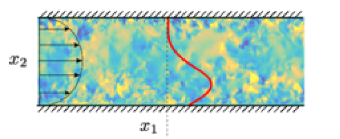
Figure 20: Alternative filter. Instantaneous wall-normal velocity used for filtering in the wall-normal direction. The red solid line represents the Gaussian kernel as a function of $x_{2}$ truncated at the wall. The colormap is the wall-normal velocity.

Figure 21 shows some examples that are practically identical to those from figure 7.

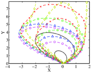
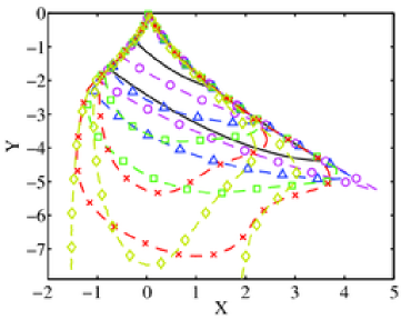
(a) (b)

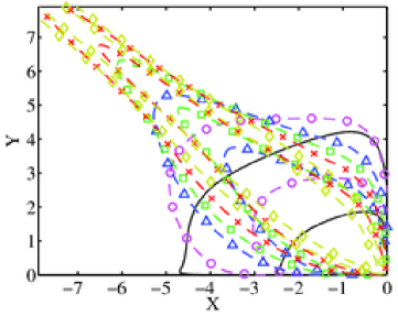
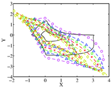
(c) (d)

Figure 21: Results filtering for the alternative filter. Joint probability density functions of (a), $R_{\omega}$–$Q_{\omega}$; (b), $R_{s}$–$Q_{s}$; (c), $Q_{s}$–$Q_{\omega}$; (d), $R_{s}$–$R_{\omega}$. Symbols and colors as in table 2. The contours contain 90% and 98% of the data.

Appendix C Conservation of probability equation

This Appendix provides some guidelines on how equation (9) is obtained. For more details about the procedure see chapter 2 in Beck & Schögl (1993). Similar equations have also been derived by Smoluchowski for the conservation of the particle probability distribution function (Doi & Edwards, 1988).

Let’s consider a number of experiments consisting of a tracer (fluid particle) in a turbulent channel flow, and its associated invariants and wall-normal position $(R,Q,x_{2})$. For simplicity, we will use $Q$ and $R$ but the following argument is also valid for $Q/Q^{\prime}$ and $R/Q^{\prime 3/2}$.

Let’s consider an initial condition for each experiment, $R$, $Q$ and the initial position of the particle, and let the system evolve in time. We will assume that the system is “mixing” (and hence ergodic), so that every sufficiently smooth initial distribution evolves to the “natural invariant density” (Beck & Schögl, 1993). That is, independently of the initial distribution of the test particles, they eventually evolve in time in such a way that they are a fair representation of the system.

Since $Q(x_{2})$ and $R(x_{2})$ are known, we can define a probability density function $P=P(R,Q,x_{2};t)$ at time $t$. The conservation of the number of experiments (equivalently of $P$) is then given by

$$\frac{\partial P}{\partial t}+\boldsymbol{\nabla}_{R,Q,x_{2}}\cdot\left(P\boldsymbol{w}\right)=0,$$ (25)

where $\boldsymbol{\nabla}_{R,Q,x_{2}}=(\partial/\partial R,\partial/\partial Q,\partial/\partial x_{2})$ and $\boldsymbol{w}$ is the mean velocity vector

$$\boldsymbol{w}=\left\langle\frac{\mathrm{D}}{\mathrm{D}t}(Q,R,x_{2})\right\rangle_{R,Q,x_{2}},$$ (26)

where $\langle\cdot\rangle_{R,Q,x_{2}}$ denotes conditional average at point $(R,Q,x_{2})$.

Let’s define a new probability

$$J=a\int_{x_{b}}^{x_{t}}P\mathrm{d}x_{2},$$ (27)

with $a=2/(x_{t}-x_{b})$. Multiplying equation (25) by $a$ and integrating from $x_{2}=x_{b}$ to $x_{2}=x_{t}$ yields to

$$\frac{\partial J}{\partial t}+\boldsymbol{\nabla}_{R,Q}\cdot\left(J\boldsymbol{V}\right)=\psi_{t}+\psi_{b},$$ (28)

where $\boldsymbol{\nabla}_{R,Q}=(\partial/\partial R,\partial/\partial Q)$, $\boldsymbol{V}$ is as defined in (3), $\psi_{b}=\alpha V_{b}J_{b}$, $\psi_{t}=-\alpha V_{t}J_{t}$ and $\alpha=1/(x_{t}-x_{b})$. $V_{b}$ and $V_{t}$ are the conditional wall-normal velocities on the $R$–$Q$ plane at $x_{2}=x_{b}$ and $x_{2}=x_{t}$, respectively, and

$$J_{b} = \frac{1}{a}P(R,Q,x_{b}),$$ (29)

$$J_{t} = \frac{1}{a}P(R,Q,x_{t}),$$ (30)

are the probability density functions of $(R,Q)$ conditioned on $x_{b}$ and $x_{t}$, respectively.

Appendix D Two examples of the conditionally averaged velocity deviation

This Appendix contains two more examples of the ratio of the magnitude of the conditionally averaged velocity deviation $\boldsymbol{v}^{\prime}$ and the mean $\boldsymbol{v}$ discussed in §3.1. Figure 22 shows two cases conditioned on the $R$–$Q$ and $R_{\omega}$–$Q_{\omega}$ planes, respectively, for case F0.1.

(a) (b)

Figure 22: Ratio of the magnitude of the conditionally averaged velocity deviation $\boldsymbol{v}^{\prime}$ and the mean $\boldsymbol{v}$, conditioned on (a), $R$–$Q$ and (b) $R_{\omega}$–$Q_{\omega}$ planes. Results for F0.1. Although the colorbar ranges from 0 to 10, values up to 100 are attained. The solid red lines in contain 90% and 98% of the data.

Appendix E Results filtering in homogeneous directions

The joint p.d.f.s from figure 7 were recomputed filtering the velocities with a Gaussian filter as the one in (7) but only applied in the two homogeneous directions. The results, shown in figure 23, are remarkable different from those in figure 7, and the mean shear never takes over as the primary effect. This difference shows that the wall-parallel filtering approach is not equivalent and justifies the complication of filtering in the wall-normal direction.

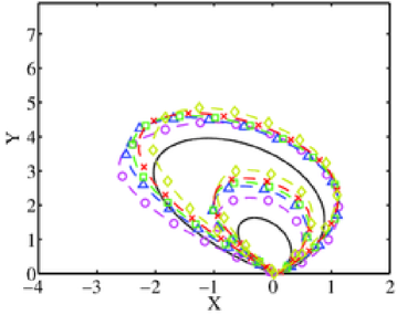
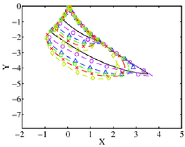
(a) (b)

(c) (d)

Figure 23: Results filtering only in the $x_{1}$ and $x_{3}$ directions. Joint probability density functions of (a), $R_{\omega}$–$Q_{\omega}$; (b), $R_{s}$–$Q_{s}$; (c), $Q_{s}$–$Q_{\omega}$; (d), $R_{s}$–$R_{\omega}$. Symbols and colors as in table 2. The contours contain 90% and 98% of the data.

References

- del Álamo et al. (2006) del Álamo, Juan C., Jiménez, Javier, Zandonade, Paulo & Moser, Robert D. 2006 Self-similar vortex clusters in the turbulent logarithmic region. J. Fluid Mech. 561, 329–358.
- Ashurst et al. (1987) Ashurst, Wm. T., Kerstein, A. R., Kerr, R. M. & Gibson, C. H. 1987 Alignment of vorticity and scalar gradient with strain rate in simulated Navier–Stokes turbulence. Phys. Fluids 30 (8), 2343–2353.
- Atkinson et al. (2012) Atkinson, C., Chumakov, S., Bermejo-Moreno, I. & Soria, J. 2012 Lagrangian evolution of the invariants of the velocity gradient tensor in a turbulent boundary layer. Phys. Fluids 24 (10).
- Batchelor & Townsend (1949) Batchelor, G. K. & Townsend, A. A. 1949 The nature of turbulent motion at large wave-numbers. Proc. Roy. Soc. London, A 199 (1057), 238–255.
- Beck & Schögl (1993) Beck, Christian & Schögl, Friedrich 1993 Thermodynamics of Chaotic Systems. Cambridge University Press, cambridge Books Online.
- Betchov (1956) Betchov, R. 1956 An inequality concerning the production of vorticity in isotropic turbulence. J. Fluid Mech. 1, 497–504.
- Blackburn et al. (1996) Blackburn, Hugh M., Mansour, Nagi N. & Cantwell, Brian J. 1996 Topology of fine-scale motions in turbulent channel flow. J. Fluid Mech. 310, 269–292.
- Borue & Orszag (1998) Borue, Vadim & Orszag, Steven A. 1998 Local energy flux and subgrid-scale statistics in three-dimensional turbulence. J. Fluid Mech. 366, 1–31.
- van der Bos et al. (2002) van der Bos, Fedderik, Tao, Bo, Meneveau, Charles & Katz, Joseph 2002 Effects of small-scale turbulent motions on the filtered velocity gradient tensor as deduced from holographic particle image velocimetry measurements. Phys. Fluids 14 (7), 2456–2474.
- Cantwell (1992) Cantwell, Brian J. 1992 Exact solution of a restricted Euler equation for the velocity gradient tensor. Phys. Fluids 4 (4), 782–793.
- Cardesa et al. (2013) Cardesa, J. I., Mistry, D., Gan, L. & Dawson, J. R. 2013 Invariants of the reduced velocity gradient tensor in turbulent flows. J. Fluid Mech. 716, 597–615.
- Cardesa et al. (2015) Cardesa, José I., Vela-Martín, Alberto, Dong, Siwei & Jiménez, Javier 2015 The propagation of kinetic energy across scales in turbulent flows. ArXiv:1505.00285v1, arXiv: 1505.00285.
- Chacin & Cantwell (2000) Chacin, Juan M. & Cantwell, Brian J. 2000 Dynamics of a low reynolds number turbulent boundary layer. J. Fluid Mech. 404, 87–115.
- Chertkov et al. (1999) Chertkov, M., Pumir, A. & Shraiman, B.I. 1999 Lagrangian tetrad dynamics and the phenomenology of turbulence. Phys. Fluids 11.
- Chevillard et al. (2011) Chevillard, Laurent, Lévêque, Emmanuel, Taddia, Francesco, Meneveau, Charles, Yu, Huidan & Rosales, Carlos 2011 Local and nonlocal pressure hessian effects in real and synthetic fluid turbulence. Phys. Fluids 23 (9).
- Chevillard & Meneveau (2006) Chevillard, L. & Meneveau, C. 2006 Lagrangian dynamics and statistical geometric structure of turbulence. Phys. Rev. Lett. 97, 174501.
- Chevillard et al. (2008) Chevillard, L., Meneveau, C., Biferale, L. & Toschi, F. 2008 Modeling the pressure hessian and viscous laplacian in turbulence: Comparisons with direct numerical simulation and implications on velocity gradient dynamics. Phys. Fluids 20 (10).
- Chong et al. (1990) Chong, M. S., Perry, A. E. & Cantwell, B. J. 1990 A general classification of three‐-dimensional flow fields. Phys. Fluids 2 (5), 765–777.
- Chong et al. (1998) Chong, M. S., Soria, J., Perry, A. E., Chacin, J., Cantwell, B. J. & Na, Y. 1998 Turbulence structures of wall-bounded shear flows found using DNS data. J. Fluid Mech. 357, 225–247.
- Corrsin (1958) Corrsin, S. 1958 Local isotropy in turbulent shear flow. Res. Memo 58B11. NACA.
- Davidson (2004) Davidson, P.A. 2004 Turbulence: An Introduction for Scientists and Engineers. OUP Oxford.
- Doi & Edwards (1988) Doi, M. & Edwards, S.F. 1988 The Theory of Polymer Dynamics. Clarendon Press.
- Elsinga & Marusic (2010) Elsinga, G. E. & Marusic, I. 2010 Evolution and lifetimes of flow topology in a turbulent boundary layer. Phys. Fluids 22 (1), 015102.
- Flores & Jiménez (2010) Flores, Oscar & Jiménez, Javier 2010 Hierarchy of minimal flow units in the logarithmic layer. Phys. Fluids 22 (7), 071704.
- Gomes-Fernandes et al. (2014) Gomes-Fernandes, R., Ganapathisubramani, B. & Vassilicos, J. C. 2014 Evolution of the velocity-gradient tensor in a spatially developing turbulent flow. J. Fluid Mech. 756, 252–292.
- Hamlington et al. (2008) Hamlington, Peter E., Schumacher, Jörg & Dahm, Werner J. A. 2008 Local and nonlocal strain rate fields and vorticity alignment in turbulent flows. Phys. Rev. E 77, 026303.
- Jiménez (1992) Jiménez, Javier 1992 Kinematic alignment effects in turbulent flows. Phys. Fluids 4 (4).
- Jiménez (2000) Jiménez, Javier 2000 Intermittency and cascades. J. Fluid Mech. 409, 99–120.
- Jiménez (2012) Jiménez, J. 2012 Cascades in wall-bounded turbulence. Ann. Rev. Fluid Mech. 44, 27–45.
- Jiménez (2013) Jiménez, J. 2013 How linear is wall-bounded turbulence? Phys. Fluids 25, 110814.
- Jiménez et al. (1993) Jiménez, Javier, Wray, Alan A., Saffman, Philip G. & Rogallo, Robert S. 1993 The structure of intense vorticity in isotropic turbulence. J. Fluid Mech. 255, 65–90.
- Kim et al. (1987) Kim, John, Moin, Parviz & Moser, Robert D 1987 Turbulence statistics in fully developed channel flow at low Reynolds number. J. Fluid Mech 177, 133–166.
- LeHew et al. (2013) LeHew, J.A., Guala, M. & McKeon, B.J. 2013 Time-resolved measurements of coherent structures in the turbulent boundary layer. Exp. Fluids 54 (4), 1–16.
- Leung et al. (2012) Leung, T, Swaminathan, N & Davidson, PA 2012 Geometry and interaction of structures in homogeneous isotropic turbulence. J. Fluid Mech. 710, 453–481.
- Li et al. (2008) Li, Yi, Perlman, Eric, Wan, Minping, Yang, Yunke, Meneveau, Charles, Burns, Randal, Chen, Shiyi, Szalay, Alexander & Eyink, Gregory 2008 A public turbulence database cluster and applications to study lagrangian evolution of velocity increments in turbulence. J. Turb. p. N31.
- Lozano-Durán et al. (2012) Lozano-Durán, Adrián, Flores, Oscar & Jiménez, Javier 2012 The three-dimensional structure of momentum transfer in turbulent channels. J. Fluid Mech. 694, 100–130.
- Lozano-Durán et al. (2015) Lozano-Durán, Adrian, Holzner, Markus & Jiménez, Javier 2015 Numerically accurate computation of the conditional trajectories of the topological invariants in turbulent flows. J. Comp. Phys. 295, 805–814.
- Lozano-Durán & Jiménez (2014a) Lozano-Durán, Adrián & Jiménez, Javier 2014a Effect of the computational domain on direct simulations of turbulent channels up to . Phys. Fluids 26 (1), 011702.
- Lozano-Durán & Jiménez (2014b) Lozano-Durán, Adrián & Jiménez, Javier 2014b Time-resolved evolution of coherent structures in turbulent channels: characterization of eddies and cascades. J. Fluid Mech. 759, 432–471.
- Lüthi et al. (2009) Lüthi, Beat, Holzner, Markus & Tsinober, Arkady 2009 Expanding the Q–R space to three dimensions. J. Fluid Mech. 641, 497–507.
- Lüthi et al. (2007) Lüthi, Beat, Ott, S., Berg, Jacob & Mann, Jakob 2007 Lagrangian multi-particle statistics. J. Turb. 8, N45, arXiv: http://dx.doi.org/10.1080/14685240701522927.
- Martín et al. (1998) Martín, Jesús, Ooi, Andrew, Chong, M. S. & Soria, Julio 1998 Dynamics of the velocity gradient tensor invariants in isotropic turbulence. Phys. Fluids 10 (9), 2336–2346.
- Marusic et al. (2013) Marusic, Ivan, Monty, Jason P., Hultmark, Marcus & Smits, Alexander J. 2013 On the logarithmic region in wall turbulence. J. Fluid Mech. 716, R3.
- Meneveau (2011) Meneveau, Charles 2011 Lagrangian dynamics and models of the velocity gradient tensor in turbulent flows. Ann. Rev. Fluid Mech. 43 (1), 219–245.
- Moisy & Jiménez (2004) Moisy, F. & Jiménez, J. 2004 Geometry and clustering of intense structures in isotropic turbulence. J. Fluid Mech. 513, 111–133.
- Moser et al. (1999) Moser, Robert D., Kim, John & Mansour, Nagi N. 1999 Direct numerical simulation of turbulent channel flow up to . Phys. Fluids 11 (4), 943–945.
- Mullin & Dahm (2006) Mullin, John A. & Dahm, Werner J. A. 2006 Dual-plane stereo particle image velocimetry measurements of velocity gradient tensor fields in turbulent shear flow. II. experimental results. Phys. Fluids 18 (3).
- Naso & Pumir (2005) Naso, Aurore & Pumir, Alain 2005 Scale dependence of the coarse-grained velocity derivative tensor structure in turbulence. Phys. Rev. E 72, 056318.
- Naso et al. (2006) Naso, Aurore, Pumir, Alain & Chertkov, Michael 2006 Scale dependence of the coarse-grained velocity derivative tensor: Influence of large-scale shear on small-scale turbulence. J. Turb. 7, N41.
- Naso et al. (2007) Naso, A., Pumir, A. & Chertkov, M. 2007 Statistical geometry in homogeneous and isotropic turbulence. J. Turb. p. N39.
- Ooi et al. (1999) Ooi, Andrew, Martín, Jesús, Soria, Julio & Chong, M. S. 1999 A study of the evolution and characteristics of the invariants of the velocity-gradient tensor in isotropic turbulence. J. Fluid Mech. 381, 141–174.
- Pumir & Naso (2010) Pumir, Alain & Naso, Aurore 2010 Statistical properties of the coarse-grained velocity gradient tensor in turbulence: Monte-carlo simulations of the tetrad model. New J. Phys. 12 (12), 123024.
- She et al. (1991) She, Zhen-Su, Jackson, Eric & Orszag, Steven A. 1991 Structure and dynamics of homogeneous turbulence: Models and simulations. Proc. Roy. Soc. London, A 434 (1890), 101–124.
- Soria et al. (1994) Soria, J., Sondergaard, R., Cantwell, B. J., Chong, M. S. & Perry, A. E. 1994 A study of the fine-‐scale motions of incompressible time-‐developing mixing layers. Phys. Fluids 6 (2), 871–884.
- Tanahashi et al. (2004) Tanahashi, M, Kang, S, Miyamoto, T & Shiokawa, S 2004 Scaling law of fine scale eddies in turbulent channel flows up to . Int. J. Heat Fluid Flow 25, 331–341.
- Tennekes & Lumley (1972) Tennekes, H. & Lumley, J.L. 1972 A First Course in Turbulence. MIT Press.
- Tsinober (1998) Tsinober, A. 1998 Is concentrated vorticity that important? Eur. J. Mech. B-Fluid 17 (4), 421–449.
- Tsinober et al. (1997) Tsinober, A, Shtilman, L & Vaisburd, H 1997 A study of properties of vortex stretching and enstrophy generation in numerical and laboratory turbulence. Fluid Dyn. Res. 21 (6), 477.
- Vieillefosse (1984) Vieillefosse, P. 1984 Internal motion of a small element of fluid in an inviscid flow. Phys. Stat. Mech. Appl. 125 (1), 150–162.
- Vieillefosse, P. (1982) Vieillefosse, P. 1982 Local interaction between vorticity and shear in a perfect incompressible fluid. J. Phys. France 43 (6), 837–842.
- Vincent & Meneguzzi (1991) Vincent, A. & Meneguzzi, M. 1991 The spatial structure and statistical properties of homogeneous turbulence. J. Fluid Mech. 225, 1–20.
- Vincent & Meneguzzi (1994) Vincent, A. & Meneguzzi, M. 1994 The dynamics of vorticity tubes in homogeneous turbulence. J. Fluid Mech. 258, 245–254.
- Wang & Lu (2012) Wang, Li & Lu, Xi-Yun 2012 Flow topology in compressible turbulent boundary layer. J. Fluid Mech. 703, 255–278.