An efficient algorithm to compute the genus of discrete surfaces and applications to turbulent flows

Abstract

A simple and efficient algorithm to numerically compute the genus of surfaces of three-dimensional objects using the Euler characteristic formula is presented. The algorithm applies to objects obtained by thresholding a scalar field in a structured-collocated grid, and does not require any triangulation of the data. This makes the algorithm fast, memory-efficient and suitable for large datasets. Applications to the characterization of complex surfaces in turbulent flows are presented to illustrate the method.

Adrián Lozano-Durán and Guillem Borrell 2015. An efficient algorithm to compute the genus of discrete surfaces and applications to turbulent flows

This work was supported by the Computational Fluid Mech. Lab. headed by Javier Jiménez, the European Research Council, under grant ERC-2010.AdG-20100224. A. Lozano–Durán was supported by an FPI fellowship from the Spanish Ministry of Education and Science, and ERC.

1 Introduction

We present a fast and memory-efficient algorithm to numerically compute the topological genus of all the surfaces associated with three-dimensional objects in a discrete space. The paper is aimed at the turbulence community interested in the topology of three-dimensional entities in turbulent flows such as coherent structures [del Álamo et al. (2006), Lozano-Durán et al. (2012)] or turbulent/non-turbulent interfaces [da Silva et al. (2014a)]. Konkle:2003 describes fast methods for computing the genus of triangulated surfaces which is usually a time and memory-consuming process. Our algorithm does not rely on triangulation [Toriwaki and Yonekura (2002), Chen and Rong (2010), Ayala et al. (2012), Cruz and Ayala (2013)] and is adapted to exploit the structured-collocated grid commonly used in the largest direct numerical simulations of turbulent flows [Kaneda et al. (2003), Hoyas and Jiménez (2008), Sillero et al. (2013)]. Our goal is to provide a clear and easy description of the algorithm and sample codes. More examples in Fortran and Python are available at torroja.

The genus is a topologically invariant property of a surface defined as the largest number of non-intersecting simple closed curves that can be drawn on the surface without separating it. The genus is negative when applied to a group of several isolated surfaces, since it is considered that no closed curves are required to separate them. Both spheres and discs have genus zero, while a torus has genus one. On the other hand, two separated spheres or the surfaces defined by a sphere shell (or sphere with an internal cavity) has genus minus one. For a set of objects in a given region, the genus is equal to the number of holes - number of objects - number of internal cavities+1. The concept is also defined for higher dimensions but the present work is restricted to two-dimensional surfaces embedded in a three-dimensional space. In Integral Geometry, the genus is part of a larger set of Galilean invariants called Minkowski functionals which characterize the global aspects of a structure in a $n$-dimensional space. The genus is also closely related to the Betti numbers, and more details can be found in tho:96.

Regarding its applications, the genus has proven to be very useful to characterize a wide variety of structures in many fields, for instance, in cosmology and related cosmic microwave background studies [J. Einasto et al. (2007)]. The large-scale structure of the universe has been studied over the years through analyses of the distribution of galaxies in three dimensions using the genus for characterizing its topology [Gott et al. (1986), Gott et al. (1987), Gott et al. (1989), Hamilton et al. (1986), Vogeley et al. (1994), Mecke et al. (1994), Park et al. (2005b), Park et al. (2005a)]. For a given threshold of the galaxy density, an isosurface separating higher and lower density regions is defined and the genus of such contour evaluated. This allows to compare the topology observed with that expected for Gaussian random phase initial conditions [Guth (1981), Linde (1983)]. In all these applications, the computation of the genus was performed by calculating the discrete integrated Gaussian curvatures [Gott et al. (1986), Chen and Rong (2010)] following the Fortran algorithm by wei:88 based on the Gauss-Bonnet theorem. As we will show in section 3, the present method does not rely on computing any curvatures.

Other applications are oriented to medical and biological areas and use the genus of surfaces or three-dimensional objects. For example, to compute adenine properties in the biochemistry field [Konkle et al. (2003)] and to evaluate the osteoporosis degree of mice femur [Martin-Badosa et al. (2003)] or human vertebrae [Odgaard and Gundersen (1993)].

The Minkowski functionals have recently been introduced in the study of turbulent flows through the so called shapefinders [Sahni et al. (1998)]. leu:swa:dav:2012 studied the topological properties of enstrophy isosurfaces in isotropic turbulence by filtering the data at different scales and computing structures of high enstrophy together with its corresponding Minkowski functionals. The geometry of the educed objects was then classified with two non-dimensional quantities, ‘planarity’ and ‘filamentarity’, which measure the shape of the structures.

In a recent work, bor:jim:2013 followed an strategy based on the genus to decide optimal thresholds in turbulent/non-turbulent interfaces extracted from numerical data. Several surfaces were obtained by thresholding the fluctuating enstrophy field in a turbulent boundary layer and their associated genus was used as an indicator of the complexity of the interface. This topological description was crucial to decide the range of thresholds where a vorticity isocontour can be considered a turbulent/non-turbulent interface.

The rest of the paper is organized as follows. Important definitions are provided in section 2. The algorithm to compute the genus is described in section 3. An alternative method is presented in §4, and validated with the previous one in section 5, which also contains some scalability tests. Two applications to turbulent flows are shown in §6. Finally, conclusions are offered in section 7.

2 Definitions

We will first introduce the definitions of object, voxel, surface, hole, cavity, and genus. The starting point is a discrete three-dimensional scalar field, $\phi=\phi(i,j,k)$, with $i=1,..,n_{x}$, $j=1,..,n_{y}$ and $k=1,..,n_{z}$, where $n_{x}$, $n_{y}$ and $n_{z}$ are the number of grid points in each direction respectively, separated by a grid spacing $\delta$. Given a thresholding value $\alpha$, we define the points belonging to the three-dimensional objects as those satisfying

$$\phi(i,j,k)>\alpha,$$ (1)

which can be expressed a scalar field $A=A(i,j,k)$ whose values are equal to 1 at $(i,j,k)$ if relation (1) is satisfied, and 0 otherwise. The latter is refer to as an empty region.

Three-dimensional individual objects in $A$ are constructed by connecting neighboring points with value 1. Figure 1(a) shows a two-dimensional example. Connectivity is defined in terms of the six orthogonal neighbors in the grid, usually called 6-connectivity. Points contiguous in oblique directions are not directly connected, although they may become so indirectly through connections with other points. This remark is important since the 6-connectivity is built-in in the algorithm and, for instance, the number of objects in the example shown in Figure 1(a) is not one but two.

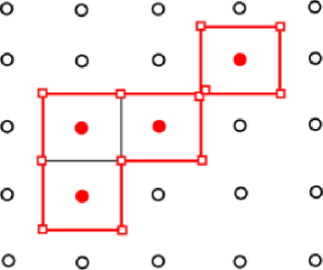
(a)             (b)

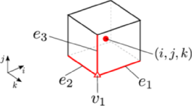
Figure 1: (a) Two-dimensional example of a structured-collocated grid defined by the open and closed circles. Points satisfying relation (1) are red closed circles and their corresponding voxels are solid lines. The exterior edges are the thicker lines colored in red and the exterior vertices are marked by squares. Objects are built by connecting orthogonal neighboring points with $A=1$, which results in two objects in this particular example. (b) Voxel around the grid point $(i,j,k)$. Only edges $e_{1}$, $e_{2}$ and $e_{3}$ (red lines), and vertex $v_{1}$ (triangle) are taken into account to compute the number of exterior vertices and edges corresponding to the voxel centered at $(i,j,k)$.

We define the voxel associated with $A(i,j,k)=1$ as the cube centered at $(i,j,k)$ and with edge length equal to $\delta$ (see Figure 1b). For a given object, its surface is delimited by the exterior faces of its voxels, i.e., those facing empty regions. In the 2D example shown in Figure 1(a), the 1D ‘surface’ is highlighted with red lines. Actual 3D examples are shown in Figure 4. A hole is a empty region piercing the object, as the torus in Figure 4(a), and a cavity an internal empty region which is locally not connected to the exterior. The term handle will be used occasionally as a synonym of hole, since they are topologically equivalent.

Our goal is to compute the genus of all the surfaces contained in $A$. Mathematically, the genus $g$ is defined in terms of the Euler characteristic $\chi$ via the relationship

$$\chi=2-2g.$$ (2)

The Euler characteristic can be calculated for continuous surfaces as

$$\chi=\frac{1}{2\pi}\iint\limits_{\Sigma}K\mathrm{d}\Sigma,$$ (3)

where $K$ is the Gaussian curvature of all the objects considered and $\Sigma$ their area. However, we are more interested in the original discrete form for polyhedral surfaces,

$$\chi=F-E+V,$$ (4)

where $F$, $E$, and $V$ are, respectively, the number of exterior faces, edges and vertices of all the polyhedra. In this case, the curvature can be considered to be located at the discrete edges, but the calculations lead to the same results as (3). The connection between the discrete and continuous formulations is the Gauss-Bonnet theorem [Chavel (2006), p. 243]. Intuitively, in terms of the elements defined above, the genus is equal to the number of holes - number of objects - number of internal cavities $+1$.

3 Algorithm

The present algorithm exploits formula (4) and the structured-collocated nature of the data to compute the genus of all the surfaces contained in the three-dimensional space defined by the scalar field $A$, without previous triangulation or calculation of the Gaussian curvatures. Note that this differs from other works which compute the genus of the three-dimensional objects themselves [Toriwaki and Yonekura (2002), Chen and Rong (2010), Ayala et al. (2012), Cruz and Ayala (2013)]. The method is conceived for large datasets of the order of $10^{2}$ GiB and takes $A$ as input.

First, we provide a general description of the algorithm. The key idea is to place a voxel around every $(i,j,k)$ point with $A(i,j,k)=1$, as the example shown in Figure 1(b), and to create a virtual mesh using the exterior elements of the resulting polyhedra. The term virtual is used here in the sense that no actual faces, vertices or edges have to be stored for each object, i.e., there is no actual structure in the code to do so, in contrast to the standard meshes obtained by triangulation, where these are saved in a file or in memory for all the objects. Figure 1(a) shows an example of a virtual mesh in a two-dimensional case.

The way to proceed is then to compute the Euler characteristic of the virtual mesh and thereafter the genus. The value of $\chi$ is easily calculated once the total number of exterior faces, vertices and edges are known for all the objects within $A$. To achieve so, three variables $F$, $V$ and $E$ are used to store the total number of exterior faces, vertices and edges, respectively, which are counted looping once through the array $A$. At each $(i,j,k)$, a voxel is placed if $A(i,j,k)=1$ and the counters $F$, $V$ and $E$ (initially set to zero) are increased accordingly every time faces, edges and vertices are identified as exterior. The selection of edges and vertices taken into account at each $(i,j,k)$, shown in Figure 1(b), is deliberately chosen to avoid counting several times edges and vertices already considered.

To prevent any problems at the boundaries of the field $A$, the original grid is extended by padding two extra planes of zeros at the beginning and at the end of each dimension. The new field will be still called $A$, but now with dimensions $N_{x}=n_{x}+4$, $N_{y}=n_{y}+4$ and $N_{z}=n_{z}+4$. For simplicity, we consider that $A$ is fully loaded in memory, but note that this is not required and it could be loaded in small chunks or planes.

A more detailed description of the algorithm is now presented:

1. Initialize the variables. $F,V$, and $E$ are integers containing the number of exterior faces, vertices and edges, and are initially set to zero. For large cases, they must be double precision. $A(i,j,k)$ is the array whose points are set to 1 if they belong to an object and to 0 otherwise. $N_{x},N_{y}$ and $N_{z}$ are the sizes of $A$ after extending it. $cube1$ and $cube2$ are auxiliary arrays of integers with dimensions $2\times 2\times 2$ and $2\times 2$, respectively, and are used to store the slices of $A$ shown in Figures 2(b,c).

2. Loop through $i=2,..,N_{x}-1$, $j=2,..,N_{y}-1$, $k=2,..,N_{z}-1$. For each $(i,j,k)$ proceed as follows:

   1. Count number of exterior faces. See algorithm 1. The six faces of the voxel at $(i,j,k)$ are considered, and its six neighbors are defined in Figure 2(a). For each neighboring voxel with coordinates $(i+\Delta i,j+\Delta j,k+\Delta k)$, $F$ is increased by one if $A(i,j,k)=1$ and $A(i+\Delta i,j+\Delta j,k+\Delta k)=0$. The possible values for $(i+\Delta i,j+\Delta j,k+\Delta k)$ are $(i-1,j,k)$, $(i+1,j,k)$, $(i,j-1,k)$, $(i,j+1,k)$, $(i,j,k-1)$ and $(i-1,j,k+1)$.

      Input: A,F

      Output: F

      if A is equal to 1 at position (i,j,k) then

            if A is equal to 0 at position (i-1,j,k) then

                 F $\leftarrow$ F + 1;

                 end if A is equal to 0 at position (i+1,j,k) then

                      F $\leftarrow$ F + 1;

                      end if A is equal to 0 at position (i,j-1,k) then

                           F $\leftarrow$ F + 1;

                           end if A is equal to 0 at position (i,j+1,k) then

                                F $\leftarrow$ F + 1;

                                end if A is equal to 0 at position (i,j,k-1) then

                                     F $\leftarrow$ F + 1;

                                     end if A is equal to 0 at position (i,j,k+1) then

                                          F $\leftarrow$ F + 1;

                                          end

      end

      ALGORITHM 1 Count number of exterior faces at position $(i,j,k)$.

   2. Count number of exterior vertices. See algorithm 2. Only vertex $v_{1}$ in Figure 1(b) is considered, and its eight adjacent voxels are defined in Figure 2(b). $V$ is increased by one if any of the eight adjacent voxels has value 1, and any other value 0. In some cases, $V$ must increase by a number $dV$ larger then 1 if some of the surrounding voxels are locally not connected. The value of $dV$ is calculated by procedure $getconnected1$, which is discussed at the end of the section.

      Input: A,V

      Output: V

      cube1 $\leftarrow$ slice of A from $i-1$ to $i$, $j-1$ to $j$ and $k-1$ to $k$;

      if any element in cube1 is 0 any element in cube1 is 1 then

            V $\leftarrow$ V + getconnected1(cube1);

           

      end

      ALGORITHM 2 Count number of exterior vertices at position $(i,j,k)$.

   3. Count number of exterior edges. See algorithm 3. Only edges $e_{1}$, $e_{2}$ and $e_{3}$ highlighted in Figure 1(b) are considered. The four adjacent voxels for edge $e_{1}$ are shown in Figure 2(c). $E$ is increased by one unit if any of the four adjacent voxels has value 1 and any other value 0. In some cases, the edges have to be counted $dE$ times when the voxels around are not locally connected. The increment $dE$ is computed by procedure $getconnected2$.

      Input: A,E

      Output: E

      cube2 $\leftarrow$ slice of A from $i-1$ to $i$, $j-1$ to $j$ and $k$;

      if any element in cube2 is 0 any element in cube2 is 1 then

            E $\leftarrow$ E + getconnected2(cube2);

           

      end

      ALGORITHM 3 Count number of exterior edges at position $(i,j,k)$.

      A similar algorithm applies to the other two edges $e_{2}$ and $e_{3}$ shown in Figure 1(b).

3. Finally the Euler characteristic and the genus are computed as $X=V-E+F$ and $G=(2-X)/2$.

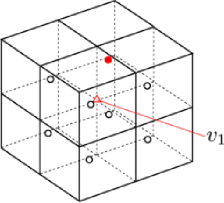
        (a)     (b)        (c)

Figure 2: Sketches of the neighboring voxels adjacent to voxel $(i,j,k)$ used to compute the number of exterior (a) faces, (b) vertices, and (c) edges. In all plots, the closed red dot denotes the center of the voxel $(i,j,k)$ and the triangle the position of its vertex $v_{1}$ as defined in Figure 1(b). Case (c) is particularized to edge $e_{1}$ and similar configurations apply to edges $e_{2}$ and $e_{3}$ (see Figure 1b).

To complete the description of the algorithm, we now comment on the procedures $getconnected1$ and $getconnected2$. Some edges or vertices has to be counted multiple times in order to be consistent with the 6-connectivity of the voxels. An example is illustrated in Figure 1(a). In contrast to other works [Toriwaki and Yonekura (2002), Ayala et al. (2012), Cruz and Ayala (2013)], this is achieved by counting the number of local objects contained in the slices shown in Figures 2(b,c), i.e., the number of objects in the $2\times 2\times 2$ sub-volume satisfying the 6-connectivity disregarding any other connections outside the slide. For example, the sub-volume denoted as C41 in Figure 3 contains one local object, and C33 contains three. Note that some voxels may be locally disconnected but belong to the same object, since they may connect indirectly through other voxels not considered in the slide. The purpose of procedure $getconnected1$, defined in algorithm 4, is to compute the number of local objects in the sub-volume shown in Figure 2(b), which can be easily obtained by any labeling method like the Hoshen-Kopelman algorithm [Hoshen and Kopelman (1976)]. Note that there is one degenerated case with a infinitesimally small hole, shown in case C63 in Figure 3, where there is only one object but the vertex must be considered twice.

Input: cube1

Output: dV

if cube1 is degenerated case C63 in Figure 3 then

      dV $\leftarrow$ 2;

      else

           dV $\leftarrow$ number of local objects in cube1;

          

end

ALGORITHM 4 Procedure getconnected1. It computes the increment $dV$ for V.

Procedure $getconnected2$ is presented in algorithm 5 and follows the same idea. In this case, the only possible configuration to obtained more than one local object in the slide shown in Figure 2(c) is with two voxels that do not share any face. In the rest of the cases, the number of local objects is one.

Input: cube2

Output: dE

if all the elements equal to 1 in cube2 are locally connected then

      dE $\leftarrow$ 1;

     

      else

           dE $\leftarrow$ 2;

          

end

ALGORITHM 5 Procedure getconnected2. It computes the increment $dE$ for E.

4 Alternative algorithm

An alternative algorithm is introduced for the purpose of validating the approach presented above. Conceptually, it follows the same ideas discussed in section 3 but relies on a pre-computed table of cases as in the work by tor:yon:2002. The process involves looping through all the vertices of the virtual grid, counting vertices, faces and edges, but no effort is made to prevent multiple counts of the last two, as opposed to the algorithm presented in section 3. This results in an extra number of faces and edges that is easily corrected by dividing the total number of faces by 4 and of edges by 2, the reason being that each face and edge contains 4 and 2 vertices, respectively.

The number of faces and edges at a particular vertex depends on its 8 surrounding voxels as shown in Figure 2(b). In this scenario, there are 256 different cases that may be reduced by symmetry to those shown in Figure 3. We will use the index $l$ to label sequentially the vertices of the virtual mesh. The contributions of the $l$-th vertex to the total number of faces, edges and vertices will be denoted by $\Delta F_{l}$, $\Delta E_{l}$ and $\Delta V_{l}$, respectively, and their values are tabulated in table 4 for all the possible cases. $F$, $E$ and $V$ are then obtained as

$$F=\frac{\sum_{l}\Delta F_{l}}{4},\quad E=\frac{\sum_{l}\Delta E_{l}}{2},\quad V=\sum_{l}\Delta V_{l},$$ (5)

where the summation extends to all the vertices of the virtual mesh. Finally, the Euler characteristic and the genus are calculated with (4) and (2), respectively.

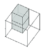
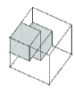
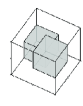
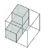
$C_{11}$ $C_{21}$ $C_{22}$ $C_{23}$ $C_{31}$

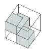
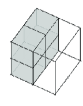
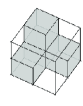
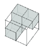
$C_{32}$ $C_{33}$ $C_{41}$ $C_{42}$ $C_{43}$

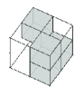
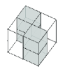
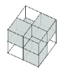
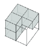
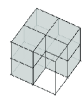
$C_{44}$ $C_{45}$ $C_{46}$ $C_{51}$ $C_{52}$

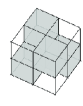
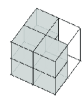
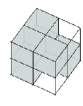
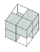
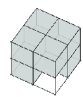
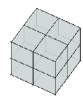
$C_{53}$ $C_{61}$ $C_{62}$ $C_{63}$ $C_{71}$ $C_{81}$

Figure 3: All possible configurations of voxels in a $2\times 2\times 2$ sub-volume considering symmetries. Grey cubes represent voxels with value one. The cases are denoted by $C_{ij}$, where $i$ is the number of voxels with value one in the sub-volume.

Contribution to the number of faces $\Delta F$, edges $\Delta E$ and vertices $\Delta F$ of each configuration of voxels in the $2\times 2\times 2$ sub-domains shown in Figure 3. Case $\Delta F$ $\Delta E$ $\Delta V$ Case $\Delta F$ $\Delta E$ $\Delta V$ $C_{01}$ 0 0 0 $C_{44}$ 8 8 2 $C_{11}$ 3 3 1 $C_{45}$ 8 8 2 $C_{21}$ 4 4 1 $C_{46}$ 12 12 4 $C_{22}$ 6 6 2 $C_{51}$ 5 5 1 $C_{23}$ 6 6 2 $C_{52}$ 7 7 1 $C_{31}$ 5 5 1 $C_{53}$ 9 9 2 $C_{32}$ 7 7 2 $C_{61}$ 4 4 1 $C_{33}$ 9 9 3 $C_{62}$ 6 6 1 $C_{41}$ 4 4 1 $C_{63}$ 6 6 2 $C_{42}$ 6 6 1 $C_{71}$ 3 3 1 $C_{43}$ 6 6 1 $C_{81}$ 0 0 0

The alternative algorithm is now briefly described following the same notation used in the previous section:

1. Initialize the variables. $F,V$, and $E$ are equivalent to those described in section 3 and are initialized to zero.

2. Loop through all the vertices in $A$. At the $l$-th vertex, proceed as follows:

   1. Find the case. Considering the 8 surrounding voxels at the $l$-th vertex shown in Figure 2(b), search for the corresponding case in Figure 3, taking into account symmetries.

   2. Contributions to $F$, $E$ and $V$. From table 4, obtain $\Delta F_{l}$, $\Delta E_{l}$ and $\Delta V_{l}$ and compute $F\leftarrow F+\Delta F_{l}$, $E\leftarrow E+\Delta E_{l}$ and $V\leftarrow V+\Delta V_{l}$.

3. Compute the actual number of faces and edges. $F\leftarrow F/4$ and $E\leftarrow E/2$.

4. Compute the Euler characteristic and genus. $X=V-E+F$ and $G=(2-X)/2$.

The algorithm described in section 3 is between 1.2 and 2 times faster than the one presented in this section, and roughly 3 times shorter in terms of lines of code, which makes it more efficient and simple to implement. For those reasons, the former approach is preferred and the alternative algorithm is only considered for validation purposes in the next section.

5 Validation and scalability

Two approaches are followed to validate the algorithms detailed in sections 3 and 4. First, synthetic cases whose genus are known beforehand are fed into the algorithms, and the results are compared to the expected theoretical values. Second, different datasets are used to compute the genus with both algorithms and the outputs are shown to match.

The synthetic cases tested are the following: all possible configurations in a $2\times 2\times 2$ volume, $n$ number of isolated solid objects ($g=-n+1$), $n$ isolated objects with an interior cavity each ($g=-2n+1$), $n$ isolated torus ($g=1$) as the example shown in Figure 4(a), and $n$ torus connected by solid bridges ($g=n$) as in Figure 4(b). More cases were tested by rotating the previous ones at different angles, for instance, as in the case shown in Figure 4(b). The values of $n$ tested range from $1$ to $10^{6}$. One more synthetic case tested consists of randomly generated structures built using the blocks shown in Figure 5, referred to as nodes and ends and linked by two type of connectors. The number of faces, edges and vertices of the resulting object is given by

$$F = n_{e}\Delta F_{e}+n_{n}\Delta F_{n}+n_{I}\Delta F_{I}+n_{II}\Delta F_{II},$$ (6)

$$E = n_{e}\Delta E_{e}+n_{n}\Delta E_{n}+n_{I}\Delta E_{I}+n_{II}\Delta E_{II},$$ (7)

$$V = n_{e}\Delta V_{e}+n_{n}\Delta V_{n}+n_{I}\Delta V_{I}+n_{II}\Delta V_{II},$$ (8)

where $n_{e}$, $n_{n}$, $n_{I}$ and $n_{II}$ are the number of ends, nodes, and connectors of type I and II that belong to the object. The increments $\Delta F_{i}$, $\Delta E_{i}$ and $\Delta V_{i}$ with $i=e,b,I$ and $II$ are the contribution to the number of faces, edges and vertices of each block respectively, and its values are tabulated in table 5. Roughly $10^{6}$ cases were randomly generated and tested and two examples are shown in Figures 4(c,d). More synthetic cases similar to those presented above but using differently shaped connectors were also successfully tested (not shown).

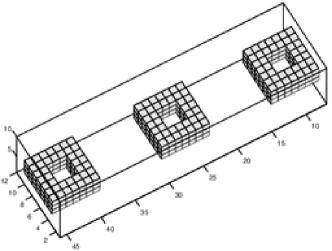
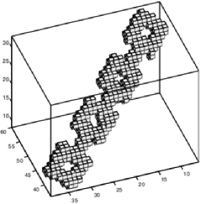
(a) (b)

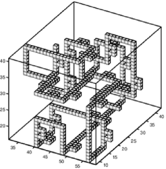
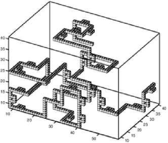
(c) (d)

Figure 4: Examples of synthetic cases used to validate the algorithms. (a), isolated torus; (b), concatenated torus; (c) and (d), synthetic random cases generated from the building blocks shown in Figure 5.

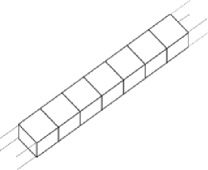
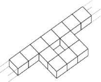
(a)       (b)       (c)       (d)

Figure 5: Building blocks of randomly generated test cases. (a), node; (b), end; (c), connector type I; (d), connector type II.

Contribution to the number of faces $\Delta F$, edges $\Delta E$ and vertices $\Delta V$ of the different blocks shown in Figure 5. Case end node connector type I connector type II $\Delta F$ 5 4 28 46 $\Delta E$ 12 12 52 88 $\Delta V$ 8 8 24 40

We perform a second validation comparing the number of faces, edges and vertices computed with the algorithm presented in section 3 and the alternative one in section 4, which of course, must be identical. This was verified for the synthetic cases described above. More test cases are the three models from the Stanford 3D Scanning Repository [Stanford (2014)] voxelized with binvox [Min (2015)] (see also noo:tur:2003) and shown in Figure 6. Finally, we tested $10^{2}$ cases delimited by a cubical region and with grid sizes from $16^{3}$ up to $4096^{3}$ whose voxels were randomly initialized with 0’s and 1’s filling approximately 50% of the total volume. Two examples are shown in Figure 7. The two algorithms yield identical results for all the cases tested, counting exactly the same number of faces, edges and vertices, and therefore, the same genus.

Table 5 summarizes the number of voxels, faces, edges, vertices and genus of some of the cases tested, which are available for download in our webpage [Lab. (2015)].

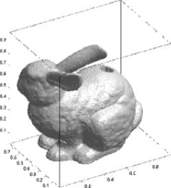
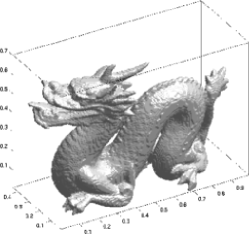
(a)    (b)    (c)

Figure 6: 3D models obtained from the Stanford 3D Scanning Repository and voxelized with binvox. (a), bunny [Turk and Levoy (1994)]; (b), Buda [Curless and Levoy (1996)]; (c), dragon [Curless and Levoy (1996)].

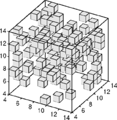
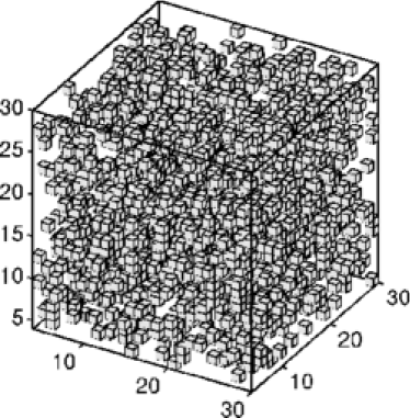
(a)    (b)

Figure 7: Test cases of cubical domains with (a), $16^{3}$ and (b), $32^{3}$ voxels randomly initialized with 0’s and 1’s.

Summary of some of the datasets tested and available for download at [Lab. (2015)] Case Size Faces Edges Vertices Genus Synthetic1 $64^{3}$ 1924 3848 1880 23 Synthetic2 $64^{3}$ 2174 4348 2120 28 Bunny $256^{3}$ 309482 618964 309466 9 Buda $256^{3}$ 129800 259600 129780 11 Dragon $256^{3}$ 164494 328988 164494 1 Random1 $64^{3}$ 297496 594992 280160 8669 Random2 $128^{3}$ 2744830 5489660 2570182 87325 Random3 $256^{3}$ 23530742 47061484 21985520 772612 Random4 $512^{3}$ 194709102 389418204 181726644 6491230 Random5 $1024^{3}$ 1584014008 3168028016 1477589086 53212462 Random6 $2048^{3}$ 12778133206 25556266412 11916193918 430969645 Random7 $4096^{3}$ 102651228492 205302456984 95713851166 3468688664

The algorithm presented in section 3 was implemented in Fortran, compiled with Intel Fortran Studio XE 2016 16.0.0 20150815 , and tested in an Intel^® Xeon^® CPU X5650 2.67GHz with 192GiB of RAM for cubical arrays of different sizes and randomly generated as those shown in table 5. The average time elapsed to compute the genus of inputs with different sizes is presented in Figure 8(a), which shows linear scalability and makes feasible applications to very large datasets.

The code was also parallelized using Fortran Coarrays. The domain decomposition was performed by dividing the $z$ direction in chunks of size $N_{x}\times N_{y}\times\Delta N_{z}$, where $\Delta N_{z}$ is nint$(N_{z}/n_{proc})$, and $n_{proc}$ the number of processing elements. Two overlapped $x$-$y$ planes are added at the beginning and end of each chunk in order to compute faces, edges and vertices without any extra communication between images. Once this is done, the genus is obtained by summing the faces, edges and vertices of all the chunks. The parallelization works for any number of processing elements smaller than $N_{z}$, and the size of the last chunk may differ from the size of the others if $N_{z}$ is not divisible by $n_{proc}$. The reader is referred to the software component of the manuscript to cover all the details of the parallelization. The strong scaling efficiency, where the problem size stays fixed but the number of processing elements increases, is shown in Figure 8(b). The results are quite satisfactory and the efficiency remains always above 90%.

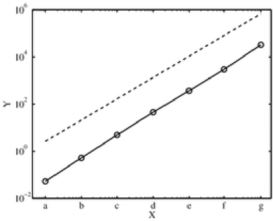
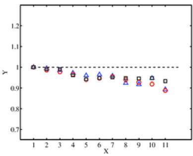
(a)       (b)

Figure 8: (a) For the Fortran serial version, average time in seconds elapsed to compute the genus of cubical arrays of size $N^{3}$ randomly initialized to 0’s and 1’s with roughly 50% of the volume occupied. Results for a single processor. The circles are the measured times and the solid dashed line is $time\sim N$. (b) For the Fortran Coarrays version, strong scaling efficiency as a function of the number of processing elements, $n_{proc}$, for three different problem sizes, $N=1024^{3}$ ($\scriptstyle\triangle$), $N=2048^{3}$ ($\circ$), and $N=4096^{3}$ ($\scriptstyle\Box$).

6 Applications to turbulent flows

We show two examples where the genus is used as a tool to characterize the topology of regions of interest in turbulent flows. In the first example, the genus is computed for millions of individual coherent structures extracted from a turbulent channel flow. In the second one, the genus is used to identify physically meaningful interfaces separating turbulent and non-turbulent flow in a time-decaying jet.

6.1 Topology of coherent regions in turbulent flows

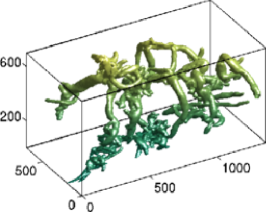
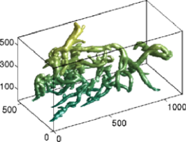
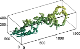
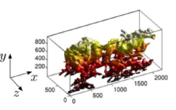
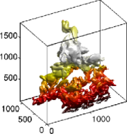
Figure 9: Examples of three vortex cluster (top row) and Q-structures (bottom row) extracted from a direct numerical simulation of a turbulent channel at $Re_{\tau}=4180$ [Lozano-Durán and Jiménez (2014)]. The flow goes from bottom-left to top-right. The axis are normalized with $\nu/u_{\tau}$. The colors change gradually with the distance to the wall, which is located at $y=0$. Note that the objects are not to scale.

We use three direct numerical simulations of turbulent channel flows (two parallel walls delimiting a flow moving on average in one direction) from loz:jim:2014 at Reynolds numbers $Re_{\tau}=934,2004$ and $4180$, with $Re_{\tau}=hu_{\tau}/\nu$ where $h$ is the channel half-height, $u_{\tau}$ the friction velocity and $\nu$ the kinematic viscosity. More details about turbulent channel flows may be found in [Chapter 7.1]pope:2000. The streamwise, wall-normal and spanwise directions are denoted by $x$, $y$ and $z$ respectively. Very briefly, we compute the genus of coherent structures, namely, regions of the flow where a variable is higher than a prescribed threshold. The three-dimensional coherent structures under study are vortex cluster from ala:jim:zan:mos:2006 and Q-structures from loz:flo:jim:2012. The former are defined in terms of the discriminant of the velocity gradient and are connected regions satisfying

$$D(x,y,z)/D^{\prime}(y)>\alpha,$$ (9)

where $D$ is the instantaneous discriminant of the velocity gradient tensor, $D^{\prime}(y)$ its standard deviation at each $x-z$ plane and $\alpha=0.02$ a thresholding parameter obtained from a percolation analysis. Similarly, Q-structures are defined as places where

$$uv(x,y,z)/uv^{\prime}(y)>H,$$ (10)

where $uv$ is the instantaneous tangential Reynolds stress, being $u$ and $v$ the streamwise and wall-normal velocity fluctuations, $uv^{\prime}(y)$ its rooted-mean-squared value at each $y$-position, and $H$ a thresholding parameter equal to $1.75$. Three-dimensional objects are constructed by connecting neighboring grid points fulfilling relations (9) for vortex clusters and (10) for Q-structures and using the 6-connectivity criteria. Full details for both types of structures can be found in ala:jim:zan:mos:2006, loz:flo:jim:2012 and loz:jim:2014. To compute the genus, each object is circumscribed within a box aligned to the Cartesian axes which constitutes the limits of the array $A(i,j,k)$ discussed in section 3. Figure 9 shows several examples of actual objects extracted from the flow and demonstrates the complex geometries that may appear. The number of structures computed is of the order of $10^{7}$, with a wide spectrum of sizes ranging from $\sim 30^{3}$ to $\sim 2000^{3}$ voxels.

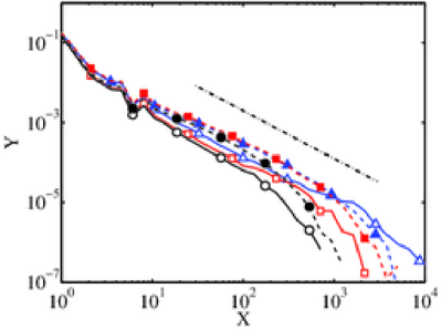
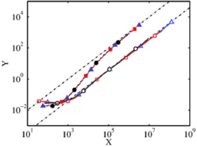
(a) (b)

Figure 10: (a) Probability density functions of the genus. The dashed-dotted line is proportional to $g^{-1.2}$. (b) Average number of holes (genus) of individual coherent structures as a function of their volume, $V_{o}$, in Kolmogorov units. The dashed-dotted lines are $\langle g\rangle=10^{-3}\eta^{-3}(V_{o}/\eta^{3})$ and $\langle g\rangle=4\times 10^{-5}\eta^{-3}(V_{o}/\eta^{3})$. For (a) and (b), the solid lines with open symbols correspond to Q-structures and the dashed lines with closed symbols to vortex clusters. Different symbols stand for different Reynolds numbers; $\circ$, $Re_{\tau}=934$; $\scriptstyle\Box$, $Re_{\tau}=2004$; $\scriptstyle\triangle$, $Re_{\tau}=4180$.

Each array $A(i,j,k)$ contains just one single object and, hence, the only contributions to the genus are the number of holes and internal cavities. The data reveals that only 0.05% of objects have negative genus and it was checked that most of structures are solid. In this scenario, genus and number of holes can be used interchangeably.

The probability density functions (PDFs) of the genus, $g$, are presented in Figure 10(a) and most of the values concentrate around zero or a few holes, although the long potential tails reach values up to $10^{4}$ holes. Figure 10(b) shows the average number of holes in the objects as a function of their volume, $V_{o}$, normalized in Kolmogorov units, $\eta^{3}$ (see [Chapter 6]pope:2000). It becomes clear that as the volume of the structures increases, so does the genus, which is reasonable if we consider that the volume of the object is related to its internal Reynolds number (or complexity), and increasing its volume results in more complicated topologies. The curves for both vortex clusters and Q-structures show good collapse for the three Reynolds numbers and follow the trend $\langle g\rangle=\rho V_{o}$, with $\langle g\rangle$ the average genus for a given volume, and $\rho$ a constant equal to $10^{-3}\eta^{-3}$ and $4\times 10^{-5}\eta^{-3}$ for vortex clusters and Q-structures respectively.

From relation $\langle g\rangle=\rho V_{o}$, the genus may be understood as an alternative method to characterize the level of complexity of the structures, with $\rho$ a density equal to the number of holes per unit volume. If we define $l$ as the average distance between holes within the structures, its value may be approximated as $l\approx(10^{-3})^{-1/\alpha_{c}}\eta\approx 30\eta$ for vortex clusters and $l\approx(4\times 10^{-5})^{-1/\alpha_{Q}}\eta\approx 90\eta$ for Q-structures, with $\alpha_{c}=2$ and $\alpha_{Q}=2.25$ the average fractal dimensions of the objects computed by loz:flo:jim:2012. These lengths are consistent with a model of coherent structures built by small blocks of length $30-90\eta$ stacked together to create larger objects but not perfectly compacted, which results in holes between the blocks. For a given volume, $V_{o}$, vortex clusters have on average 25 times more holes than Q-structures, suggesting that their blocks and connections are fundamentally different. This is consistent with loz:flo:jim:2012 who showed that the Q-structures are flake-shaped while vortex clusters are worm-shaped, also visible in Figure 9.

6.2 Turbulent/non-turbulent interface detection in a turbulent jet

We use a direct numerical simulation of a time-decaying turbulent jet (see [Chapter 5]pope:2000) by vel:bor:2014 to identify a turbulent/non-turbulent interface. A brief introduction about such interface is presented next.

Two regions can be distinguished in an unbounded turbulent flow, the fully turbulent region, characterized by strong fluctuations, and the irrotational free stream. These two regions are, in most cases, separated by a single thin layer, called turbulent/non-turbulent interface. The first step to analyze the physical processes that happen within this interface layer is to locate it. This interface is known to be fractal-like [Sreenivasan et al. (1989)] and it contains all the scales between the smallest and the largest possible. Such a wide range of scales imposes a strong restriction on the size of the domain that has to be studied, since small portions would only give reliable results for the small scales. The most common method to locate the turbulent/non-turbulent interface is to threshold a scalar field where the two characteristic states of the flow can be easily distinguished. Sre:1989 and FLM:5919136 use the concentration of a passive scalar injected in the turbulent side, and threshold it at the least probable value of the concentration. FLM:95049 and SilvaTaveira use a particular isocontour of the magnitude of vorticity $|\omega|(x,y,z)=\omega_{0}$, where vorticity is defined as the rotational of the velocity vector, $\vec{\omega}=\nabla\wedge\vec{u}$. gampert2014vorticity found that the isocontours obtained thresholding concentration and vorticity magnitude are similar, and dasilva2014characteristics found that the least probable value of vorticity magnitude can be used successfully as a threshold for a variety of turbulent flows. Despite the convergence of some popular methodologies, other authors like FLM:9176488 have proposed alternative strategies.

                 (a)                  (b)                  (c)

Figure 11: Isocontours of vorticity magnitude $|\omega|$, at different thresholds for a turbulent jet. Figure (a) corresponds to a very low value of the threshold $|\omega|/\omega_{rms}=0.05$, and very low genus, where $\omega_{rms}$ is the rooted-mean-squared vorticity magnitude. Figure (b) corresponds to the threshold that maximize the genus $|\omega|/\omega_{rms}=3$, and (c) to a threshold slightly higher than (b) $|\omega|/\omega_{rms}=5$.

One important aspect of the choice of the threshold is the impact it has on the geometry of the interface. If the threshold $\omega_{0}$ is a low value of vorticity, like the detection shown in Figure 11(a), the interface is relatively simple, showing that the perturbation caused by the turbulent motion is smoothed out farther down the free stream. On the other hand, as soon as the threshold is slightly increased, the surface is populated with a large amount of handles (or holes), as can be seen in Figures 11(b,c). These handles are most likely a geometrical feature of the fully turbulent flow. Depending on the value of the threshold, the surface generated has different topological properties.

The geometrical complexity, measured in this case with the number handles, has an important side effect on the analysis of the properties of the flow depending on the relative position to the interface. Two relatively popular assumptions about the interface are that there is a privileged direction across which the relative distance to the interface can be measured [Westerweel et al. (2009), da Silva and Taveira (2010)], and that the interface is simple enough so that a local normal is meaningful [Bisset et al. (2002), Chauhan et al. (2014)]. These two assumptions are not strictly correct if handles are a dominant feature of the interface. At the same time, the criterion explored by dasilva2014characteristics depends on the characteristics of the non-turbulent region. The probability density function of vorticity in the same round jet of Figure 11 is shown in Figure 12. It has been premultiplied to emphasize the fact that the PDF has two major contributions, one from the bulk of the non-turbulent flow with low vorticity (left peak), and a second one from the bulk of the turbulent flow with high vorticity (right peak). Note that, if the flow was in an ideal state with no perturbations, the left peak would be in in the limit of vanishing vorticity. In consequence, the outcome of the criterion defined by [Sreenivasan et al. (1989)] applied to the vorticity field can be intuitively defined as the lowest threshold that is not affected by the spurious vorticity present in the free stream. This criterion is strictly correct, but it may be more representative of the smoothed out perturbations relatively far from the turbulent motion. It is therefore necessary to explore other complementary threshold choices that provide a more complete description of the vorticity field.

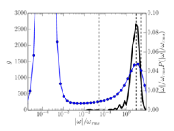
Figure 12: (Blue line with circles) Premultiplied PDF of vorticity magnitude $|\omega|$ normalized with its root-mean-squared value in a turbulent temporal round jet. (Solid black line) Genus of the turbulent/non-turbulent interface as a function of the vorticity magnitude. The vertical dashed lines are the thresholds used in Figures 11(a,b,c).

The genus of the surface detected as a function of the value used to threshold the vorticity magnitude is presented in Figure 12. The results have been averaged using an ensemble of four equivalent cases. The curve shows that there is a gradual yet evident change in the topological properties of the vorticity interface from a threshold $\omega_{0}\sim\omega_{rms}$. Beyond that value, handles are a dominant feature of the interface, and the standard tools for the conditional analysis are probably not valid. If the criterion of minimum probability provides a lower limit for the threshold, the genus of the interface is an useful criterion for an upper limit.

7 Conclusions

We have presented and validated a simple algorithm to numerically compute the genus of discrete surfaces using the Euler characteristic formula. The method is valid for surfaces associated with three-dimensional objects obtained by thresholding a discrete scalar field defined in a structured-collocated grid and offers several advantages. First, it does not rely on any direct triangulation of the surfaces, which is usually memory and time-consuming. Besides, the surfaces of all the 3D objects in the domain are automatically detected and the genus is exactly computed without any spurious holes. Last, but not least, it needs practically zero memory, it is fast and scalable, with a computational cost directly proportional to the size of the grid computed. The algorithm is also highly parallelizable, and a Fortran Coarrays version was implemented to take advantage of multicore processors without increasing the memory usage. This makes the algorithm suitable for large datasets, like the ones encountered in direct numerical simulations of turbulent flows. Two applications to the characterization of complex structures in turbulent flows have been presented. In the first case, the genus of coherent structures extracted from a turbulent channel flows is computed and found to be proportional to the volume of the objects. In the second application, the genus is used to find an appropriate threshold to detect the turbulent/non-turbulent interface in a turbulent jet.

The authors would like to acknowledge fruitful discussions with Javier Jiménez and José Cardesa-Dueñas, and to thank Profs. Dolors Ayala and Irving Cruz for providing the test data used in the early stages of the work. We are also very grateful to Tim Hopkins for his assistance with the software component of the paper, and to the referees for their very constructive feedback.

References

- [1]
- Ayala et al. (2012) D. Ayala, E. Vergés, and I. Cruz. 2012. A Polyhedral Approach to Compute the Genus of a Volume dataset, In Proceedings of the International Conference on Computer Graphics Theory and Applications-GRAPP 2012. INSTICC Press (February 2012), 38–47.
- Bisset et al. (2002) D. K. Bisset, J. C. R. Hunt, and M. M. Rogers. 2002. The turbulent/non-turbulent interface bounding a far wake. Journal of Fluid Mechanics 451 (1 2002), 383–410. DOI:http://dx.doi.org/10.1017/S0022112001006759
- Borrell and Jimenez (2013) G. Borrell and J. Jimenez. 2013. Geometrical properties and scaling of the turbulent-nonturbulent interface in boundary layers. Bulletin of the American Physical Society. 66th Annual Meeting of the APS, Division of Fluid Dynamics. 58, 18 (2013).
- Chauhan et al. (2014) K. Chauhan, J. Philip, C. M. de Silva, N. Hutchins, and I. Marusic. 2014. The turbulent/non-turbulent interface and entrainment in a boundary layer. Journal of Fluid Mechanics 742 (3 2014), 119–151. DOI:http://dx.doi.org/10.1017/jfm.2013.641
- Chavel (2006) I. Chavel. 2006. Riemannian Geometry (second ed.). Cambridge University Press. http://dx.doi.org/10.1017/CBO9780511616822 Cambridge Books Online.
- Chen and Rong (2010) L. Chen and Y. Rong. 2010. Digital topological method for computing genus and the Betti numbers. Topology and its Applications 157, 12 (2010), 1931 – 1936. DOI:http://dx.doi.org/10.1016/j.topol.2010.04.006
- Cruz and Ayala (2013) I. Cruz and D. Ayala. 2013. An Efficient Alternative to Compute the Genus of Binary Volume Models, In Proceedings of the International Conference on Computer Graphics Theory and Applications-GRAPP 2013. INSTICC Press (February 2013), 18–26.
- Curless and Levoy (1996) B. Curless and M. Levoy. 1996. A Volumetric Method for Building Complex Models from Range Images. In Proceedings of the 23rd Annual Conference on Computer Graphics and Interactive Techniques (SIGGRAPH ’96). ACM, New York, NY, USA, 303–312. DOI:http://dx.doi.org/10.1145/237170.237269
- da Silva et al. (2014a) C. B. da Silva, J. C. Hunt, I. Eames, and J. Westerweel. 2014a. Interfacial Layers Between Regions of Different Turbulence Intensity. Ann. Rev. Fluid Mech. 46, 1 (2014), 567–590. DOI:http://dx.doi.org/10.1146/annurev-fluid-010313-141357
- da Silva and Taveira (2010) C. B. da Silva and R. R. Taveira. 2010. The thickness of the turbulent/nonturbulent interface is equal to the radius of the large vorticity structures near the edge of the shear layer. Physics of Fluids 22 (2010), 121702.
- da Silva et al. (2014b) C. B. da Silva, R. R. Taveira, and G. Borrell. 2014b. Characteristics of the turbulent/nonturbulent interface in boundary layers, jets and shear-free turbulence. In J Phys, Vol. 506. IOP Publishing, 012015.
- del Álamo et al. (2006) J. C. del Álamo, J. Jiménez, P. Zandonade, and R. D. Moser. 2006. Self-similar vortex clusters in the turbulent logarithmic region. J. Fluid Mech. 561 (8 2006), 329–358. DOI:http://dx.doi.org/10.1017/S0022112006000814
- Gampert et al. (2014) M. Gampert, J. Boschung, F. Hennig, M. Gauding, and N. Peters. 2014. The vorticity versus the scalar criterion for the detection of the turbulent/non-turbulent interface. J Fluid Mech 750 (2014), 578–596.
- Gott et al. (1986) J. R. Gott, III, M. Dickinson, and A. L. Melott. 1986. The sponge-like topology of large-scale structure in the universe. Astrophys. J 306 (July 1986), 341–357. DOI:http://dx.doi.org/10.1086/164347
- Gott et al. (1989) J. R. Gott, III, J. Miller, T. X. Thuan, S. E. Schneider, D. H. Weinberg, C. Gammie, K. Polk, M. Vogeley, S. Jeffrey, S. P. Bhavsar, A. L. Melott, R. Giovanelli, M. P. Hayes, R. B. Tully, and A. J. S. Hamilton. 1989. The topology of large-scale structure. III - Analysis of observations. Astrophys. J 340 (may 1989), 625–646. DOI:http://dx.doi.org/10.1086/167425
- Gott et al. (1987) J. R. Gott, III, D. H. Weinberg, and A. L. Melott. 1987. A quantitative approach to the topology of large-scale structure. Astrophys. J 319 (aug 1987), 1–8. DOI:http://dx.doi.org/10.1086/165427
- Guth (1981) A. H. Guth. 1981. Inflationary universe: A possible solution to the horizon and flatness problems. Phys. Rev. D 23 (Jan 1981), 347–356. Issue 2. DOI:http://dx.doi.org/10.1103/PhysRevD.23.347
- Hamilton et al. (1986) A. J. S. Hamilton, J. R. Gott, III, and D. Weinberg. 1986. The topology of the large-scale structure of the universe. Astrophys. J 309 (oct 1986), 1–12. DOI:http://dx.doi.org/10.1086/164571
- Hoshen and Kopelman (1976) J. Hoshen and R. Kopelman. 1976. Percolation and cluster distribution. I. Cluster multiple labeling technique and critical concentration algorithm. Phys. Rev. B 14 (Oct 1976), 3438–3445. Issue 8. DOI:http://dx.doi.org/10.1103/PhysRevB.14.3438
- Hoyas and Jiménez (2008) S. Hoyas and J. Jiménez. 2008. Reynolds number effects on the Reynolds-stress budgets in turbulent channels. Physics of Fluids 20, 10 (2008), –. DOI:http://dx.doi.org/10.1063/1.3005862
- J. Einasto et al. (2007) J. Einasto, M. Einasto, E. Tago, E. Saar, G. Hütsi, M. Jõeveer, L. J. Liivamägi, I. Suhhonenko, J. Jaaniste, P. Heinämäki, V. Müller, A. Knebe, and D. Tucker. 2007. Superclusters of galaxies from the 2d redshift survey. A&A 462, 2 (2007), 811–825. DOI:http://dx.doi.org/10.1051/0004-6361:20065296
- Kaneda et al. (2003) Y. Kaneda, T. Ishihara, M. Yokokawa, K. Itakura, and A. Uno. 2003. Energy dissipation rate and energy spectrum in high resolution direct numerical simulations of turbulence in a periodic box. Physics of Fluids 15, 2 (2003).
- Konkle et al. (2003) S. E. Konkle, P. Moran, B. Hamann, and K. Joy. 2003. Fast Methods for Computing Isosurface Topology with Betti Numbers. Kluwer Academic Publishers, Norwell, Massachusetts, 363–375.
- Lab. (2015) C. F. M. Lab. 2015. Algorithm for computing the genus: codes and datasets. (2015). http://torroja.dmt.upm.es/genus/
- Leung et al. (2012) T. Leung, N. Swaminathan, and P. A. Davidson. 2012. Geometry and interaction of structures in homogeneous isotropic turbulence. J. Fluid Mech. 710 (11 2012), 453–481. DOI:http://dx.doi.org/10.1017/jfm.2012.373
- Linde (1983) A. Linde. 1983. Chaotic inflation. Phys. Lett. 129, 3–4 (1983), 177 – 181. DOI:http://dx.doi.org/10.1016/0370-2693(83)90837-7
- Lozano-Durán et al. (2012) A. Lozano-Durán, O. Flores, and J. Jiménez. 2012. The three-dimensional structure of momentum transfer in turbulent channels. J. Fluid Mech. 694 (3 2012), 100–130. DOI:http://dx.doi.org/10.1017/jfm.2011.524
- Lozano-Durán and Jiménez (2014) A. Lozano-Durán and J. Jiménez. 2014. Effect of the computational domain on direct simulations of turbulent channels up to . Phys. Fluids 26, 1 (2014), 011702. DOI:http://dx.doi.org/10.1063/1.4862918
- Martin-Badosa et al. (2003) E. Martin-Badosa, A. Elmoutaouakkil, S. Nuzzo, D. Amblard, L. Vico, and F. Peyrin. 2003. A method for the automatic characterization of bone architecture in 3D mice microtomographic images. Comput Med Imag Grap 27, 6 (2003), 447–458.
- Mecke et al. (1994) K. R. Mecke, T. Buchert, and H. Wagner. 1994. Robust morphological measures for large-scale structure in the Universe. aap 288 (Aug. 1994), 697–704.
- Min (2015) P. Min. 2015. binvox: mesh voxelizer. (2015). http://www.google.com/search?q=binvox
- Nooruddin and Turk (2003) F. Nooruddin and G. Turk. 2003. Simplification and repair of polygonal models using volumetric techniques. Visualization and Computer Graphics, IEEE Transactions on 9, 2 (April 2003), 191–205. DOI:http://dx.doi.org/10.1109/TVCG.2003.1196006
- Odgaard and Gundersen (1993) A. Odgaard and H. Gundersen. 1993. Quantification of connectivity in cancellous bone, with special emphasis on 3-D reconstructions. Bone 14, 2 (1993), 173 – 182. DOI:http://dx.doi.org/10.1016/8756-3282(93)90245-6
- Park et al. (2005a) C. Park, Y.-Y. Choi, M. S. Vogeley, J. R. Gott, III, J. Kim, C. Hikage, T. Matsubara, M.-G. Park, Y. Suto, D. H. Weinberg, and SDSS Collaboration. 2005a. Topology Analysis of the Sloan Digital Sky Survey. I. Scale and Luminosity Dependence. Astrophys. J 633 (Nov. 2005), 11–22. DOI:http://dx.doi.org/10.1086/452625
- Park et al. (2005b) C. Park, J. Kim, and J. R. Gott, III. 2005b. Effects of Gravitational Evolution, Biasing, and Redshift Space Distortion on Topology. Astrophys. J 633 (Nov. 2005), 1–10. DOI:http://dx.doi.org/10.1086/452621
- Pope (2000) S. Pope. 2000. Turbulent Flows. Cambridge University Press.
- Sahni et al. (1998) V. Sahni, B. S. Sathyaprakash, and S. F. Shandarin. 1998. Shapefinders: A New Shape Diagnostic for Large-Scale Structure. Astrophys. J 495, 1 (1998), L5.
- Sillero et al. (2013) J. A. Sillero, J. Jiménez, and R. D. Moser. 2013. One-point statistics for turbulent wall-bounded flows at Reynolds numbers up to +≈ 2000. Physics of Fluids 25, 10 (2013), 105102.
- Sreenivasan et al. (1989) K. R. Sreenivasan, R. Ramshankar, and C. Meneveau. 1989. Mixing, Entrainment and Fractal Dimensions of Surfaces in Turbulent Flows. Proceedings of the Royal Society of London. A. Mathematical and Physical Sciences 421, 1860 (1989), 79–108. DOI:http://dx.doi.org/10.1098/rspa.1989.0004
- Stanford (2014) Stanford. 2014. The Stanford 3D Scanning Repository. (2014). https://graphics.stanford.edu/data/3Dscanrep/
- Thompson (1996) A. C. Thompson. 1996. Minkowski geometry (1. publ. ed.). Cambridge University Press,, Cambridge [u.a.].
- Toriwaki and Yonekura (2002) J. Toriwaki and T. Yonekura. 2002. Euler Number and Connectivity Indexes of a Three Dimensional Digital Picture. Forma 17 (2002), 183–209.
- Turk and Levoy (1994) G. Turk and M. Levoy. 1994. Zippered Polygon Meshes from Range Images. In Proceedings of the 21st Annual Conference on Computer Graphics and Interactive Techniques (SIGGRAPH ’94). ACM, New York, NY, USA, 311–318. DOI:http://dx.doi.org/10.1145/192161.192241
- Vela-Martín and Borrell (2014) A. Vela-Martín and G. Borrell. 2014. Computation of a temporal decaying turbulent jet with GPGPUS. Computational Fluid Mechanics Group. UPM. Internal Report (2014).
- Vogeley et al. (1994) M. S. Vogeley, C. Park, M. J. Geller, J. P. Huchra, and J. R. Gott, III. 1994. Topological analysis of the CfA redshift survey. Astrophys. J 420 (Jan. 1994), 525–544. DOI:http://dx.doi.org/10.1086/173583
- Weinberg (1988) D. H. Weinberg. 1988. Contour - A topological analysis program. Publications of the Astronomical Society of the Pacific 100 (Nov. 1988), 1373–1385. DOI:http://dx.doi.org/10.1086/132337
- Westerweel et al. (2009) J. Westerweel, C. Fukushima, J. M. Pedersen, and J. C. R. Hunt. 2009. Momentum and scalar transport at the turbulent/non-turbulent interface of a jet. Journal of Fluid Mechanics 631 (7 2009), 199–230. DOI:http://dx.doi.org/10.1017/S0022112009006600