Achieving robust and high-fidelity quantum control via spectral phase optimization

Abstract

Achieving high-fidelity control of quantum systems is of fundamental importance in physics, chemistry and quantum information sciences. However, the successful implementation of a high-fidelity quantum control scheme also requires robustness against control field fluctuations. Here, we demonstrate a robust optimization method for control of quantum systems by optimizing the spectral phase of an ultrafast laser pulse, which is accomplished in the framework of frequency domain quantum optimal control theory. By incorporating a filtering function of frequency into the optimization algorithm, our numerical simulations in an abstract two-level quantum system as well as in a three-level atomic rubidium show that the optimization procedure can be enforced to search optimal solutions while achieving remarkable robustness against the control field fluctuations, providing an efficient approach to optimize the spectral phase of the ultrafast laser pulse to achieve a desired final quantum state of the system.

Keywords: quantum optimal control theory, quantum state transfer, ultrafast laser pulse, adiabatic pulses

1 Introduction

In spite of rapid progress in quantum technology [1], it remains a challenge to achieve high-fidelity quantum control while tolerating uncertainty and quantum decoherence effects [2, 3]. In regard to the latter, the advanced ultrafast (pico-, femto- and attosecond) laser technique provides an alternative approach to control quantum dynamical processes on extremely short time scales before quantum decoherence effect plays roles, leading to a variety of applications from science to industry [4, 5, 6, 7, 8]. Mathematical description of an ultrafast laser pulse can be written as

$$\mathcal{E}(t)=\mathrm{Re}\Bigg{[}\int_{0}^{\infty}\boldsymbol{E}(\omega)\exp(-i\omega t)d\omega\Bigg{]},$$ (1)

in terms of a complex function $\boldsymbol{E}(\omega)$ in the frequency domain, where $\boldsymbol{E}(\omega)=\mathcal{A}(\omega)\exp(i\phi(\omega))$ is a product of a spectral amplitude $\mathcal{A}(\omega)$ and a spectral phase $\phi(\omega)$. To achieve high-fidelity of quantum control with optimal ultrafast laser pulses, quantum optimal control experiment (QOCE) relying on the computational intelligence of an evolutionary algorithm is often employed to find the “best” combination of $\mathcal{A}(\omega)$ and $\phi(\omega)$ in the frequency domain [9, 10, 11, 12], whereas many quantum optimal control theory (QOCT) methods used for simulations are accomplished in the time domain by directly shaping the temporal field $\mathcal{E}(t)$ [3, 13, 14]. It is clear that there is a big mismatch between theory and experiment. Recently, a general frequency domain quantum optimal control theory (FDQOCT) was established [15, 16], which can be utilized in a monotonic convergence fashion to optimize the spectral field $\boldsymbol{E}(\omega)$ while incorporating multiple internal limitations as well as external constraints into the optimization algorithm. Provided that the involved limitations and constraints are sufferable, the broad successes of QOCT and QOCE applications have shown that there usually exist many solutions capable of achieving the same observable value [17, 18, 19, 20]. A question of particular interest is how to search optimal robust solutions against various uncertainties. Many efforts have been put forth to address this question even for the simplest quantum system of two states [21, 22, 23, 24, 25, 26, 27, 28, 29, 30, 31, 32, 33]. Optimization approaches usually are accomplished in the time domain by solving a robust optimization problem [34, 35, 36, 37, 38], which have intuitive applications with state-of-the-art technologies for microsecond radio-frequency pulses.
In this paper, we present a theoretical investigation in the framework of FDQOCT for optimal robust control of quantum systems without taking the uncertainty into account. To highlight quantum coherence effects while reducing the “search space” [39, 40, 41, 42, 43, 44], the FDQOCT is specifically employed to shape the spectral phase $\phi(\omega)$ of an ultrafast nonadiabatic pulse by keeping the spectral amplitude $\mathcal{A}(\omega)$ unchanged, which leads to the spectral-phase-only optimization (SPOO) algorithm. To illustrate this method without complexities from the dimension of systems, we first employ the SPOO algorithm to obtain a complete population inversion between two levels, for which previous theoretical and experimental studies have demonstrated that a quadratic spectral phase function of $\phi(\omega)=\beta_{0}/2(\omega-\omega_{0})^{2}$ with a large enough chirp rate $\beta_{0}$ can lead to robust control [45, 46, 47, 48]. By incorporating a smooth filtering function of frequency into the optimization algorithm, our numerical simulations show that optimal solutions towards remarkable robustness also turn out to be a quadratic spectral phase function, whereas optimal solutions found by the algorithm in the absence of this filtering function are far from being robust. From quantum optimal control point of view, our results provide a new approach to search optimal robust solutions, yielding the high-fidelity value of a cost functional while resisting the control field fluctuations. We further examine the SPOO algorithm in a three-level atomic rubidium, for which optimal robust solutions are unknown before performing the optimization. Two different schemes of quantum state transfer are discussed for achieving optimal robust population inversion between levels with either allowed or forbidden electric dipole transitions.
The rest of the paper is organized as follows. In Sec. 2, we describe the details of the SPOO algorithm in the frame of FDQOCT. Numerical simulations and discussion are demonstrated in Sec. 3 for the two-level quantum system and three-level atomic rubidium. Our results are briefly summarized in Sec. 4.

2 Theoretical Methods

Consider a general system consisting of $N$ quantum states $|n\rangle$ with eigenenergies $|E_{n}\rangle$ ($n=1\cdots$, $N$). The total Hamiltonian operator $\hat{H}(t)$ of the quantum system in interaction with the temporal field $\mathcal{E}(t)$ can be described by $\hat{H}(t)=\hat{H}_{0}-\hat{\mu}\mathcal{E}(t)$, where $\hat{H}_{0}=\Sigma_{n=1}^{N}E_{n}|n\rangle\langle n|$ is the field-free Hamiltonian operator and $\hat{\mu}$ denotes the dipole operator. The time-dependent evolution of the quantum system initially in state $|i\rangle$ at time $t_{i}$ is described by the wave function $|\Psi(t)\rangle=\hat{U}(t,t_{i})|i\rangle$. The corresponding unitary evolution operator $\hat{U}(t,t_{i})$ is governed by the time-dependent Schrödinger equation,

$$i\hbar\frac{\partial\hat{U}(t,t_{i})}{\partial t}=\hat{H}(t)\hat{U}(t,t_{i}),\ \ \ \hat{U}(t_{i},t_{i})\equiv\mathbb{I}.$$ (2)

To find an optimal control field $\mathcal{E}(t)$ in the ultrafast time scales, the FDOQCT has been formulated previously in Ref. [15] for optimizing the complex function $\boldsymbol{E}(\omega)$ subject to multiple equality constraints, which was further developed in Ref. [16] leading to a multi-objective frequency domain optimization algorithm. In the following, we will describe the details of how employ the FDQOCT to optimize the real spectral phase function $\phi(\omega)$ of an ultrafast control field subject to multiple equality constraints. As a result, a multiple-equality-constraint SPOO algorithm is used for maximizing a cost functional $P_{i\rightarrow f}(t_{f})=|\langle f|\Psi(t_{f})\rangle|^{2}$, i.e., the probability of quantum state transfer from the initial state $|i\rangle$ to the final state $|f\rangle$ at the final time $t_{f}$.
As demonstrated in the FDOQCT [15], a dummy variable $s\geq 0$ is employed to record the changes of the spectral phase $\phi(\omega)$ and the cost functional $P_{i\rightarrow f}(t_{f})$ with $\phi(s,\omega)$ and $P_{i\rightarrow f}(s,t_{f})$. Note that the parameter $s$ introduced in the FDQOCT is not a physical variable of the laser field, which is used for formulating the optimization algorithm by first-order differential equations [49, 50]. As $s$ increases, updating the spectral phase from $\phi(s,\omega)$ to $\phi(s+\delta s,\omega)$ that increases the value of $P_{i\rightarrow f}(t_{f})$ (i.e., $P_{i\rightarrow f}(s+\delta s,t_{f})-P_{i\rightarrow f}(s,t_{f})\geq 0$) can be written using the chain rule as

$$g_{0}(s)\equiv\frac{dP_{i\rightarrow f}(s,t_{f})}{ds}=\int_{0}^{\infty}\frac{\delta P_{i\rightarrow f}(s,t_{f})}{\delta\phi(s,\omega)}\frac{\partial\phi(s,\omega)}{\partial s}d\omega\geq 0.$$ (3)

If there are no any constraints on the optimal control fields, Eq. (3) can be satisfied by integrating the following equation

$$\frac{\partial\phi(s,\omega)}{\partial s}=\frac{\delta P_{i\rightarrow f}(s,t_{f})}{\delta\phi(s,\omega)}.$$ (4)

In this work, we further impose two equality external constraints

$$g_{1}(s)\equiv\frac{d\mathcal{E}(s,t_{i})}{ds}=\int_{0}^{\infty}\frac{\delta\mathcal{E}(s,t_{i})}{\delta\phi(s,\omega)}\frac{\partial\phi(s,\omega)}{\partial s}d\omega=0,$$ (5)

and

$$g_{2}(s)\equiv\frac{d\mathcal{E}(s,t_{f})}{ds}=\int_{0}^{\infty}\frac{\delta\mathcal{E}(s,t_{f})}{\delta\phi(s,\omega)}\frac{\partial\phi(s,\omega)}{\partial s}d\omega=0,$$ (6)

on the control fields during the whole optimization, which are often considered in quantum optimal control simulations for practical implementation [13, 28, 38, 51, 52]. Optimal solutions of $\partial\phi(s,\omega)/\partial s$ that simultaneously satisfy Eqs. (3), (5) and (6) can be expressed as

$$\frac{\partial\phi(s,\omega)}{\partial s}=g_{0}(s)\int_{0}^{\infty}S(\omega^{\prime}-\omega)\sum_{\ell=0}^{2}\left[\Gamma^{-1}\right]_{0\ell}\frac{\delta\mathcal{Q}_{\ell}}{\delta\phi(s,\omega)}d\omega^{\prime},$$

where $\mathcal{Q}_{0}=P_{i\rightarrow f}(s,t_{f})$, $\mathcal{Q}_{1}=\mathcal{E}(s,t_{i})$ and $\mathcal{Q}_{2}=\mathcal{E}(s,t_{f})$. A frequency domain convolution filtering function $S(\omega^{\prime}-\omega)$ in Eq. (2) is introduced to locally average the inputs $\delta\mathcal{Q}_{\ell}/\delta\phi(s,\omega)$. In our simulations, we take a normalized Gaussian function of frequency as the convolution filtering

$$S(\omega^{\prime}-\omega)=\exp\Bigg{[}-\frac{4\ln 2(\omega^{\prime}-\omega)^{2}}{\sigma^{2}}\Bigg{]},$$ (8)

where $\sigma$ is the bandwidth. Although such a convolution filtering has been involved in the FDQOCT [15, 16], we did not highlight its virtue for obtaining robust solutions. $\Gamma$ is a $3\times 3$ symmetric matrix composed of the elements

$$\Gamma_{\ell\ell^{\prime}}=\int_{0}^{\infty}\delta\mathcal{Q}_{\ell}/\delta\phi(s,\omega)\int_{0}^{\infty}S(\omega^{\prime}-\omega)\delta\mathcal{Q}_{\ell^{\prime}}/\delta\phi(s,\omega^{\prime})d\omega^{\prime}d\omega.$$ (9)

By inserting Eq. (2) into Eqs. (3), (5) and (6), we can verify that

$$g_{\ell^{\prime}}(s) = g_{0}(s)\int_{0}^{\infty}\delta\mathcal{Q}_{\ell^{\prime}}/\delta\phi(s,\omega)\int_{0}^{\infty}S(\omega^{\prime}-\omega)\sum_{\ell=0}^{2}\left[\Gamma^{-1}\right]_{0\ell}\frac{\delta\mathcal{Q}_{\ell}}{\delta\phi(s,\omega)}d\omega^{\prime}d\omega$$ (10)

$$= g_{0}(s)\sum_{\ell=0}^{M}\left[\Gamma^{-1}\right]_{0\ell}\Gamma_{\ell\ell^{\prime}}$$

$$= g_{0}(s)\delta_{0\ell^{\prime}}\ \ \ \ell^{\prime}=0,1,2.$$

That is, all requirements from Eqs. (3), (5) and (6) are satisfied during the optimization simultaneously if the spectral phase is updated with the algorithm Eq. (2).
The SPOO algorithm in Eq. (2) is independent of the dimension of Hamiltonian, ensuring its applicability to complex multi-level quantum systems. To perform this SPOO algorithm, the gradients $\delta\mathcal{Q}_{1}/\delta\phi(s,\omega)$ and $\delta\mathcal{Q}_{2}/\delta\phi(s,\omega)$ can be analytically given by

$$\frac{\partial\mathcal{E}(s,t)}{\partial\phi(s,\omega)}=\mathcal{A}(\omega)\sin[\omega t-\phi(s,\omega)]$$ (11)

with $t=t_{i}$ and $t_{f}$. The gradient $\delta\mathcal{Q}_{0}/\delta\phi(s,\omega)$ is computed by

$$\frac{\delta\mathcal{Q}_{0}}{\delta\phi(s,\omega)}=\int_{-\infty}^{\infty}\frac{\delta\mathcal{Q}_{0}}{\delta\mathcal{E}(s,t)}\frac{\partial\mathcal{E}(s,t)}{\partial\phi(s,\omega)}dt,$$ (12)

in which $\partial\mathcal{E}(s,t)/\partial\phi(s,\omega)$ has been derived in Eq. (11), and the gradient $\delta\mathcal{Q}_{0}/\delta\mathcal{E}(s,t)$ is calculated by [53]

$$\frac{\delta\mathcal{Q}_{0}}{\delta\mathcal{E}(s,t)} = -2\mathrm{Im}\left\{\langle i|\hat{U}^{\dagger}(t_{f},t_{i})|f\rangle\langle f|\hat{U}(t_{f},t_{i})\hat{U}^{\dagger}(t,t_{i})\hat{\mu}\hat{U}(t,t_{i})|i\rangle\right\}.$$ (13)

In our simulations, the spectral amplitude $\mathcal{A}(\omega)$ is fixed with a Gaussian frequency distribution centered at the frequency $\omega_{0}$,

$$\mathcal{A}(\omega)=\mathcal{E}_{0}\sqrt{\frac{1}{2\pi\Delta\omega^{2}}}\exp\Bigg{[}-\frac{(\omega-\omega_{0})^{2}}{2\Delta\omega^{2}}\Bigg{]},$$ (14)

where $\Delta\omega$ is the frequency bandwidth, and $\mathcal{E}_{0}$ is the peak field strength. Equation (2) is firstly solved by using a temporal field $\mathcal{E}(s_{0},t)$ with an initial guess of the spectral phase $\phi(s_{0},\omega)$, and then the generated wavefunction $|\Psi(t)\rangle$ is used to calculate $\delta\mathcal{Q}_{0}/\delta\phi(s_{0},\omega)$. The first-order differential equation (2) is solved (e.g., by using the Euler method) to obtain the first updated spectral phase $\phi(s_{1}=s_{0}+\delta s,\omega)=\phi(s_{0},\omega)+\delta s(\partial\phi(s_{0},\omega)/\partial s)$, which combined with the fixed spectral amplitude $\mathcal{A}(\omega)$ is used to calculate the first updated control field $\mathcal{E}(s_{1},t)$. Equation (2) is further solved by using the updated field $\mathcal{E}(s_{1},t)$, which will increase the cost functional of $\mathcal{Q}_{0}$ (i.e., $P_{i\rightarrow f}(t_{f})$) as compared with that by the initial field $\mathcal{E}(s_{0},t)$. By repeating the step $s_{0}$ to the step $s_{1}$, the spectral phase is iteratively updated from $\phi(s_{1},\omega)$ to $\phi(s_{2}=x_{1}+\delta s,\omega),\cdots,\phi(s_{n},\omega)$ until $\mathcal{Q}_{0}$, i.e., $P_{i\rightarrow f}(t_{f})$, converges to the desired precision.

3 Results and Discussion

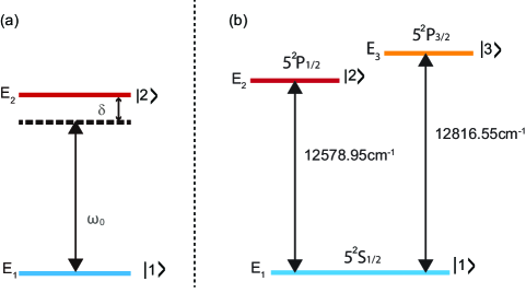
Figure 1: Schematic energy level structures of a two-level quantum system (a) and a three-level atomic rubidium (b). For two-level simulations, the energies of the two states $|1\rangle$ and $|2\rangle$ in (a) are fixed at $E_{1}=0$ and $E_{2}=12500$ cm^-1, and $\delta$ denotes a single-photon detuning between the center frequency $\omega_{0}$ and the transition frequency $\omega_{12}=(E_{2}-E_{1})/\hbar$. For three-level simulations, the three states $|1\rangle$, $|2\rangle$ and $|3\rangle$ correspond to the energy levels $5^{2}S_{1/2}$, $5^{2}P_{1/2}$ and $5^{2}P_{3/2}$ in atomic rubidium with the energies $E_{1}=0$, $E_{2}=12578.95$ and $E_{3}=12816.55$ cm^-1, respectively.

In the following, we will perform the SPOO algorithm in an abstract two-level quantum system and in a three-level atomic rubidium, respectively. For two-level simulations, the energies of the two states $|1\rangle$ and $|2\rangle$ in Fig. 1 (a) are fixed at $E_{1}=0$ and $E_{2}=12500$ cm^-1, and $\delta$ denotes a single-photon detuning between the center frequency $\omega_{0}$ and the transition frequency $\omega_{12}=(E_{2}-E_{1})/\hbar$. The transition dipole moments between the states $|1\rangle$ and $|2\rangle$ are chosen to be $\mu_{12}=\mu_{21}=1.0$ a.u. without loss of generality. For three-level simulations, the three states $|1\rangle$, $|2\rangle$ and $|3\rangle$ in Fig. 1 (b) correspond to the energy levels $5^{2}S_{1/2}$, $5^{2}P_{1/2}$ and $5^{2}P_{3/2}$ for atomic rubidium-87 with $E_{1}=0$, $E_{2}=12578.95$ and $E_{3}=12816.55$ cm^-1, respectively. The transition dipole moments between states are taken as $\mu_{12}=\mu_{21}=2.9931$ and $\mu_{13}=\mu_{31}=4.2275$ a.u., and $\mu_{23}=\mu_{32}$ are set to be zero for describing the electric dipole forbidden atomic transitions between the states $|2\rangle$ and $|3\rangle$.

3.1 Application to an abstract two-level quantum system

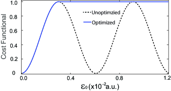
Figure 2: Two-level simulations: The cost functional $P_{1\rightarrow 2}(t_{f})$ as a function of the field strength $\mathcal{E}_{0}$ by using the transform limited (dashed lines) and spectral phase optimized (solid line) pulses. The optimized calculations are accomplished by optimizing the spectral phase without involving the filtering function $S(\omega^{\prime}-\omega)$ in Eq. (2) while fixing the spectral amplitude $\mathcal{A}(\omega)$ as the corresponding transform limited pulse.

We first perform the two-level simulations by using a zero spectral phase and fixing the center frequency $\omega_{0}$ in resonance with the transition frequency $\omega_{12}$, for which the temporal control field in Eq. (1) corresponds to a transform limited pulse, $\mathcal{E}(t)=\mathcal{E}_{0}\exp(-t^{2}/2\tau_{0}^{2})\cos\omega_{0}t$ with a duration of $\tau_{0}=1/\Delta\omega$. In our simulations, the total propagation time is taken as $T=t_{f}-t_{i}=100\tau_{0}=1000$ fs, which is discretized with $3.2\times 10^{5}$ uniform time steps. The quantum system is initially in the state $|1\rangle$, and finally is expected to be in the state $|2\rangle$. We scan the field strength $\mathcal{E}_{0}$ with different values to solve the time-dependent Schrödinger equation (2), and the corresponding $P_{1\rightarrow 2}(t_{f})$ as a function of $\mathcal{E}_{0}$ is plotted in Fig. 2 (dashed lines). Since the exact resonant condition (i.e., $\delta=0$) is satisfied, the transition probability $P_{1\rightarrow 2}(t_{f})$ can be analytically expressed as [54] $P_{1\rightarrow 2}(t_{f})=\sin^{2}(A(t_{f})/2)$ with $A(t_{f})=\mathcal{E}_{0}\mu_{12}\int_{t_{i}}^{t_{f}}\exp(-t^{2}/2\tau_{0}^{2})/2dt\propto\mathcal{E}_{0}$, which as shown in Fig. 2 oscillates between 0 and 1 depending on the value of $\mathcal{E}_{0}$. Complete population transfer occurs for $A(t_{f})=(2q+1)\pi$ (i.e., odd-$\pi$ pulse) and complete population return takes place for $A(t_{f})=2q\pi$ (i.e., even-$\pi$ pulse), where $q$ is an integer. This phenomenon is either called Rabi oscillation or Rabi flopping. The odd-$\pi$ pulse provides an approach for achieving complete population transfer, whereas as demonstrated in Fig. 2 the obtained population of $P_{1\rightarrow 2}(t_{f})$ is not robust with respect to the fluctuation of $\mathcal{E}_{0}$. To explore whether there are optimal robust solutions, the SPOO algorithm is first employed without using the filtering function $S(\omega^{\prime}-\omega)$. Optimal spectral phases with different values of $\mathcal{E}_{0}$ are obtained, and the corresponding $P_{1\rightarrow 2}(t_{f})$ as a function of $\mathcal{E}_{0}$ is plotted in Fig. 2 (solid line). It is clear that $P_{1\rightarrow 2}(t_{f})$ with a high-fidelity is possible in a large range of $\mathcal{E}_{0}$ (i.e. $A(t_{f})\geq\pi$). That is, there exist many optimal spectral phases $\phi(\mathcal{E}_{0},\omega)$, which are able to obtain the observable value of $P_{1\rightarrow 2}(t_{f})>0.9999$ with an admissible error $<10^{-4}$.

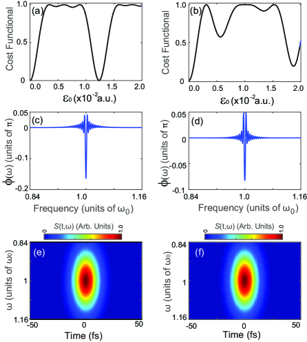
Figure 3: Two-level simulations: Robustness with respect to the field strength variations for two different optimal spectral phases. (a) and (b) The cost functional $P_{1\rightarrow 2}(t_{f})$ as a function of $\mathcal{E}_{0}$, (c) and (d) the corresponding spectral phases, and (e) and (f) the time and frequency resolved distributions of the control fields. The two optimized spectral phases are obtained from the unfiltered optimizations at $\mathcal{E}_{0}=0.6\times 10^{-2}$ (left panels) and $1.0\times 10^{-2}$ a.u. (right panels).

To see whether the optimized spectral phases are robust, two different optimized spectral phases obtained with $\mathcal{E}_{0}=0.6\times 10^{-2}$ and $1.0\times 10^{-2}$ a.u. that lead to $P_{1\rightarrow 2}(t_{f})>0.9999$ in Fig. 2 are examined, respectively. The corresponding robustness of $P_{1\rightarrow 2}(t_{f})$ against the fluctuation of $\mathcal{E}_{0}$ is plotted in Figs. 3 (a) and (b). As can be seen from Figs. 3 (c) and (d), the optimized spectral phases are mainly modulated in a small region around the center frequency $\omega_{0}$, showing strong oscillations in the values. Figures 3 (e) and (f) plot the corresponding time and frequency resolved distributions of the control fields, which are almost unchanged as compared with the corresponding transform limited pulses. That is, the optimized spectral phases only lead to a small modulation on the initial temporal field, but such a slight modification of the initial guess (i.e., a transform limited pulse) is capable of maximizing $P_{1\rightarrow 2}(\mathcal{E}(\cdot))$. We also examine other optimized spectral phases (not shown here), showing similar behaviours as Fig. 3. Thus, the SPOO algorithm in the absence of the filtering function can be used to find optimal solutions, but they are far from being robust.

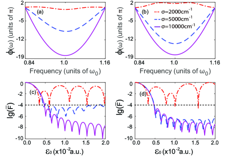
Figure 4: Two-level simulations: The effect of the parameter $\sigma$ on the optimal spectral phases and infidelity $\bar{F}=1-P_{1\rightarrow 2}(t_{f})$. The optimal spectral phases for three different values of $\sigma=2.0\times 10^{3},5.0\times 10^{3}$ and $1.0\times 10^{4}$ cm^-1 are calculated with (a) $\mathcal{E}_{0}=0.6\times 10^{-2}$ and (b) $1.0\times 10^{-2}$ a.u., and the corresponding infidelity $\bar{F}=1-P_{1\rightarrow 2}(t_{f})$ in decimal logarithmic scale as a function of $\mathcal{E}_{0}$ is plotted in (c) and (d). The dashed horizontal lines correspond to the infidelity $\bar{F}=1.0\times 10^{-4}$.

We apply the SPOO algorithm with the filtering function to the above problem. To show the role of the parameter $\sigma$ in the filtering function, we examine the optimization algorithm at the two different field strengths $\mathcal{E}_{0}=0.6\times 10^{-2}$ and $1.0\times 10^{-2}$ a.u. as used in the above simulations with different values of $\sigma=2.0\times 10^{3},5.0\times 10^{3}$ and $1.0\times 10^{4}$ cm^-1, and the corresponding optimal spectral phases are plotted in Figs. 4 (a) and (b). We can find that the optimal spectral phases are very sensitive to the parameter $\sigma$, indicating that there are still many optimal solutions with the same spectral amplitude $\mathcal{A}(\omega)$. To clearly view the dependance of the robustness on the parameter $\sigma$ with these optimal spectral phases, Figs. 4 (c) and (d) show the corresponding infidelity $\bar{F}=1-P_{1\rightarrow 2}(t_{f})$ in decimal logarithmic scale as a function of $\mathcal{E}_{0}$, which usually is used to assess a quantum state transformation error in quantum information science. We find that the infidelity is dramatically decreased to the admissible error below $10^{-4}$ with the value of $\sigma\geq 5.0\times 10^{3}$ cm^-1, where the corresponding optimal spectral phases in Figs. 4 (a) and (b) show a smooth change in $\omega$ without strong oscillations.

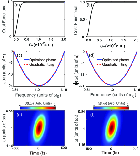
Figure 5: Two-level simulations: Robustness with respect to the field strength variations for two different optimal spectral phases. (a) and (b) The cost functional $P_{1\rightarrow 2}(t_{f})$ as a function of $\mathcal{E}_{0}$, (c) and (d) the corresponding spectral phases, and (e) and (f) the time and frequency resolved distributions of the control fields. The two optimized spectral phases (blue solid lines) are obtained from the filtered optimizations at $\mathcal{E}_{0}=0.6\times 10^{-2}$ (left panels) and $1.0\times 10^{-2}$ a.u. (right panels), which with a constant shift can be fitted (red dashed lines) by using a quadratic function of $\beta_{0}/2(\omega-\omega_{0})^{2}$ with a chirp rate $\beta_{0}=898$ fs² in (c) and 1044 fs² in (d).

Figure 5 displays the same simulations as Fig. 3 by involving the filtering function with the parameter of $\sigma=2.0\times 10^{4}$ cm^-1. The robustness against $\mathcal{E}_{0}$ is examined in Figs. 5 (a) and (b) with the two optimized spectral phases in Figs. 5 (c) and (d), showing remarkable robustness to large changes in the field strength $\mathcal{E}_{0}$. It is interesting to note that optimized spectral phases with a constant shift can be fitted very well using a quadratic spectral phase $\beta_{0}/2(\omega-\omega_{0})^{2}$ with a chirp rate $\beta_{0}$, which clearly introduces a time-dependent frequency distribution of the field, as shown in Figs. 5 (e) and (f) and prolongs the durations $\tau$ of the optimized pulses much longer than $\tau_{0}=10$ fs. As a result, shaping the spectral phase will reduce the peak intensity of the optimized temporal electric fields as compared with the transform-limited pulse (see also details in Appendix). The underlying mechanism of generating robust control of a two-level quantum system with such a linear frequency-chirped pulse can be understood well in terms of the noncrossing adiabatic representation (see details in Appendix). As demonstrated in Figs. 6 (a) and (b), the evolution of quantum systems is almost completely in the adiabatic ground state $|-\rangle$ during the whole quantum control process. As a result, the quantum system in the diabatic representation smoothly evolves from the initial state $|1\rangle$ to the final state $|2\rangle$, as shown in Figs. 6 (c) and (d). That is, an adiabatic pulse is designed by optimizing the spectral phase of the initial nonadiabatic ultrafast pulse, which leads to a remarkable robustness against the variations of the field strength.

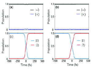
Figure 6: Two-level simulations: Time evolution of the qubit control in (a) and (b) adiabatic and (c) and (d) diabatic states for the two filtered spectral phase-optimized pulses. The spectral amplitude $A(\omega)$ is fixed at (left panels) $\mathcal{E}_{0}=0.6\times 10^{-2}$ and (right panels) $1.0\times 10^{-2}$ a.u.

Optimal control theory combined with adiabatic theorem has been applied previously for the time-domain design of adiabatic microsecond radio-frequency pulses by explicitly incorporating an adiabaticity term into the cost functional [35]. The present method is performed in the frequency domain for the design of ultrafast pulses without using such an adiabaticity term as the part of control objective, whereas as demonstrated in the two-level simulations the spectral filtering function with a large enough value of $\sigma$ “implicitly” enforces optimal solutions towards adiabatic pulses, providing a new approach to search for optimal robust solutions.

3.2 Application to a three-level atomic rubidium

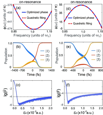
Figure 7: Three-level simulations for on-resonance excitations: The center frequency $\omega_{0}$ is fixed in resonance with the transition frequency $\omega_{12}=(E_{2}-E_{1})/\hbar$ in (left panels) and $\omega_{13}=(E_{3}-E_{1})/\hbar$ (right panels). (a) and (d): The optimal spectral phases (blue solid lines) are obtained with $\mathcal{E}_{0}=0.8\times 10^{-2}$ a.u. and $\sigma=1.8\times 10^{4}$ cm^-1, which with a constant shift are fitted (red dashed lines) by using a quadratic function $\beta_{0}/2(\omega-\omega_{c})^{2}$ (a) with $\omega_{c}=12727.39$ cm^-1 and $\beta_{0}=4161$ fs² and (d) with $\omega_{c}=12644.675$ cm^-1 and $\beta_{0}=-2235$ fs². (b) and (e): The time-dependent population transfer among the three states. (c) and (f): The infidelity $\bar{F}=1-P_{1\rightarrow 2}(t_{f})$ and $\bar{F}=1-P_{1\rightarrow 3}(t_{f})$ in decimal logarithmic scale as a function of $\mathcal{E}_{0}$. The dashed horizontal lines correspond to the infidelity $\bar{F}=1.0\times 10^{-4}$.

3.2.1 On-resonance case

We apply the SPOO algorithm with the filtering function to the three-level atomic rubidium, as shown in Fig. 1 (b). We first examine two different on-resonance excitation schemes from state $|1\rangle$ by fixing the center frequency $\omega_{0}$ in resonance with the transition frequency $\omega_{12}=(E_{2}-E_{1})/\hbar$ or $\omega_{13}=(E_{3}-E_{1})/\hbar$, and the corresponding final state is $|2\rangle$ or $|3\rangle$, respectively. Figure 7 shows the corresponding simulations with $\mathcal{E}_{0}=0.8\times 10^{-2}$ a.u. and $\sigma=1.8\times 10^{4}$ cm^-1. The optimal spectral phase in Fig. 7 (a) or in Fig. 7 (d) with a constant shift in the value can be fitted very well by using a quadratic function $\beta_{0}/2(\omega-\omega_{c})^{2}$ centered at the frequency $\omega_{c}$. Figure 7 (c) or (e) shows the corresponding infidelity $\bar{F}=1-P_{1\rightarrow 2}(t_{f})$ or $\bar{F}=1-P_{1\rightarrow 3}(t_{f})$ in decimal logarithmic scale as a function of $\mathcal{E}_{0}$. A high fidelity with the admissible error of $\bar{F}<10^{-4}$ is observed in a large range of $\mathcal{E}_{0}$. We also examine this on-resonance case with other values of $\mathcal{E}_{0}$, and the similar behaviours are observed with a large value of $\sigma$. We can see that the frequency distribution of the optimal spectral phase is not symmetric to the center frequency $\omega_{0}$, and therefore a frequency detuned quadratic spectral phase function is found as an optimal robust solution. As can be seen from Fig. 7 (b) or from Fig. 7 (e), the state $|3\rangle$ or $|2\rangle$ is clearly involved in the population transfer process, whereas the final population in this state is efficiently suppressed to a very low value of $<10^{-4}$. Furthermore, we can find in Fig. 7 (c) or in Fig. 7 (f) that increasing the laser pulse strength causes a rising trend of infidelity. This can also be attributed to the existence of the state $|3\rangle$ or $|2\rangle$, as the frequency bandwidth of the pulse is broad enough to excite both the excited states $|2\rangle$ and $|3\rangle$ with an energy separation of $E_{3}-E_{2}\approx 238$ cm^-1. Based on these considerations, the optimal robust pulse does not construct an adiabatic passage between the initial state and the final state, whereas it is able to achieve a high-fidelity of $P_{1\rightarrow 2}(t_{f})>0.9999$ or $P_{1\rightarrow 3}(t_{f})>0.9999$ against the fluctuation of $\mathcal{E}_{0}$.
For such a three-level atomic rubidium, we have noticed that the three levels involved can also be approximated to form a two-level system with the states $|1\rangle$ and $|2\rangle$ by choosing a set of optimal parameters ($\Delta\omega,\delta$, $\beta_{0}$) [47], so that the effect of the state $|3\rangle$ on quantum state transfer can be sufficiently suppressed. That is, we may also form a two-level system by setting the spectral amplitude $\mathcal{A}(\omega)$ with the frequency bandwidth $\Delta\omega$ small enough to overlap significantly only the final state of interest [45]. As a result, optimal robust solutions will turn out to be the two-level case with adiabatic pulses. That is, the dynamics of a multi-level quantum system is reduced to an effective two-level model.

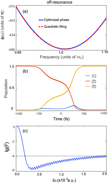
Figure 8: Three-level simulations for off-resonance excitations: The system is initially in the sate $|2\rangle$ with the state $|3\rangle$ as the target, and the center frequency $\omega_{0}$ is fixed in resonance with the transition frequency $\omega_{12}=(E_{2}-E_{1})/\hbar$. (a): The optimal spectral phase (blue solid line) is obtained with $\mathcal{E}_{0}=0.8\times 10^{-2}$ a.u. and $\sigma=1.8\times 10^{4}$ cm^-1, which with a constant shift is fitted (red dashed lines) by using a quadratic function $\beta_{0}/2(\omega-\omega_{c})^{2}$ with $\omega_{c}=12735.2$ cm^-1 and $\beta_{0}=3884$ fs². (b): The time-dependent population transfer among the three states. (c): The corresponding infidelity $\bar{F}=1-P_{2\rightarrow 3}(t_{f})$ in decimal logarithmic scale as a function of $\mathcal{E}_{0}$. The dashed horizontal lines correspond to the infidelity $\bar{F}=1.0\times 10^{-4}$.

3.2.2 Off-resonance case

Figure 8 shows the off-resonance case in the three-level atomic rubidium with $\mathcal{E}_{0}=0.8\times 10^{-2}$ a.u. and $\sigma=1.8\times 10^{4}$ cm^-1. For this off-resonance excitation, we assume that the initial state is $|2\rangle$, and fix the center frequency $\omega_{0}$ in resonance with the transition frequency $\omega_{12}=(E_{2}-E_{1})/\hbar$. An optimal spectral phase, as shown in Fig. 8 (a), is found, which leads to the evolution of the system from the initial state $|2\rangle$ to the final state $|3\rangle$. The optimal spectral phase with a constant shift in the value can also be fitted very well by using a quadratic function $\beta_{0}/2(\omega-\omega_{c})^{2}$. Although the direct transition between the states $|2\rangle$ and $|3\rangle$ is forbidden, the intermediate state $|1\rangle$ due to the broad bandwidth of the pulse can be involved to construct two (multi)-photon transition pathways. As can be seen from Fig. 8 (b), the population is transferred to this intermediate state. Note that the population transfer processes involved in this three-level system are different from that by using the stimulated adiabatic Raman passage (STIRAP) scheme within a V-type configuration system, where the intermediate state is never populated during the whole population transfer process [55, 56]. Thus, this is not a completely adiabatic quantum state transfer from the initial state to the final state by using the optimized pulse, whereas we can see that the population in the intermediate state $|1\rangle$ is not noticeable during the population transfer process. As a result, it is still able to lead to a very low error in a large range of $\mathcal{E}_{0}$.
Finally, we have an analysis for the center frequency detuning $\omega_{c}-\omega_{0}$ involved in the both on- and off-resonance simulations. We can expand the optimal spectral phase around the center frequency $\omega_{0}$ by using the second-order Taylor expansion $\phi(\omega)=\Sigma_{n=0}^{2}(\phi_{n}/n!)(\omega-\omega_{0})^{n}$, where the first-order term is involved to lead to a shift of the spectral phase shape in the frequency domain. According to the Fourier transform shift theorem, a linear term in the spectral phase leaves the control field envelope unchanged, and only shifts the pulse in the time domain. As a result, the optimal solutions can also be understood as the chirped pulses, which transform an initial quantum state into a desired final state through an intermediate state by sweeping instantaneous frequency of laser pulse.

4 Conclusion

In summary, we have demonstrated a theoretical study to show how the spectral phase of an ultrafast laser pulse can be shaped to achieve optimal robust control of quantum systems without shaping the spectral amplitude of the laser pulse. A SPOO algorithm was established in the framework of FDQOCT, and was successfully applied for quantum state transfer in the abstract two-level quantum system as well as in the three-level atomic rubidium. By incorporating the filtering function into the optimization algorithm, the optimal spectral phases that lead to robust and high-fidelity quantum state transfer are found, and therefore we have shown an efficient approach to enforce optimal control algorithm in the frequency domain to extract optimal robust solutions.
As this frequency domain optimization approach is in line with the current ultrafast pulse shaping technique commonly used in QOCEs, this work together with optimization algorithms may open a new access to achieve optimal robust feedback control of quantum systems, for which both the spectral phase and amplitude of the ultrafast laser pulses can be used as the control variables. This method in principle can be potentially applied to more complex quantum control problems by either increasing the dimensionality of quantum systems or considering interactions of quantum systems with its environments, e.g., electron spins in diamond [61], single molecules in polymer hosts polymers [62], and therefore we expect that it can be used in a robust way to optimize specific pathways in chemical reactions and energy transfer channels in light-harvesting complexes, to achieve various quantum gates for quantum computing.

5 Acknowledgment

Y.G. is partially supported by the scholarship of Hunan Provincial Department of Education of China under grant No. 2015210, and by Hunan Provincial Natural Science Foundation of China under grant No. 2017JJ2272. C.C.S acknowledges the financial support by the Vice-Chancellor’s Postdoctoral Research Fellowship of University of New South Wales (UNSW), Australia. D.D. acknowledges partial supports by the Australian Research Council under Grant No. DP130101658. Y.G. also acknowledges the support and hospitality provided by UNSW Canberra during his visit.

Appendix

The time-dependent electric field of a chirped pulse with a quadratic spectral phase takes the form [57]

$$\mathcal{E}\left(t\right)=\mathcal{E}_{0}\mathrm{Re}\left\{\sqrt{\frac{\tau_{0}^{2}}{\tau_{0}^{2}-i\beta_{0}}}\exp\left[-\frac{t^{2}}{2\tau^{2}}-i\left(\frac{\beta}{2}t+\omega_{0}\right)t\right]\right\},$$ (15)

where $\beta=\beta_{0}/(\tau_{0}^{4}+\beta_{0}^{2})$ and $\tau=\tau_{0}\sqrt{1+\beta_{0}^{2}/\tau_{0}^{4}}$. By substituting the complex-valued $\sqrt{\tau_{0}^{2}/(\tau_{0}^{2}-i\beta_{0})}=fe^{-i\varphi}$ into Eq. (15), the time-dependent electric field $\mathcal{E}\left(t\right)$ can be written as

$$\mathcal{E}\left(t\right)=\mathcal{E}^{\prime}_{0}\left\{\exp\left(-\frac{t^{2}}{2\tau^{2}}\right)\cos\left[\left(\frac{\beta}{2}t+\omega_{0}\right)t+\varphi\right]\right\}$$ (16)

with an updated field strength $\mathcal{E}^{\prime}_{0}=\mathcal{E}_{0}f$.

Within the rotating wave approximation, the diabatic interaction Hamiltonian can be described by

$$\hat{H}_{dia}=\frac{\hbar}{2}\left(\begin{array}[]{cc}-\Delta(t)&\Omega(t)\exp(i\varphi)\\ \Omega(t)\exp(-i\varphi)&\Delta(t)\\ \end{array}\right),$$ (19)

where $\Delta(t)=\delta-\beta t$ is the instantaneous detuning and $\Omega(t)=-\mu_{12}\mathcal{E}^{\prime}_{0}\exp(-t^{2}/2\tau^{2})/\hbar$ is the Rabi frequency. This leads to a modified Landau-Zener model with a constant variation rate $\beta$ of the energy difference [58, 59], whereas the time-dependent diabatic coupling $\Omega(t)$ is involved. Clearly, the diabatic energy levels in the absence of $\Omega(t)$ will take place an exact crossing when the energy level is swept. In the presence of $\Omega(t)$, however, the adiabatic energy levels $E_{\pm}(t)=\pm\hbar\sqrt{\Omega^{2}(t)+\Delta^{2}(t)}/2$ obtained by diagonalizing $\hat{H}_{dia}$ will form an avoided crossing by slowly chirping the instantaneous frequency of the control field with a large enough chirp rate $\beta_{0}$ combined with a large enough Rabi frequency $\Omega(t)$, i.e., the adiabatic condition of $|\dot{\vartheta}(t)|\ll\sqrt{\Delta^{2}(t)+\Omega^{2}(t)}$ is maintained [29, 46, 60]. The corresponding adiabatic eigenstates can be given by $|+\rangle=\sin\vartheta(t)|1\rangle e^{i\varphi}+\cos\vartheta(t)|2\rangle$ and $|-\rangle=\cos\vartheta(t)|1\rangle e^{i\varphi}-\sin\vartheta(t)|2\rangle$ with a mixing angle $\vartheta(t)=\tan^{-1}(\Omega(t)/\Delta(t))/2$.

References

References

- [1] Castelvecchi D 2017 Quantum computers ready to leap out of the lab in 2017 Nature 541 9
- [2] Gottesman D 2016 Efficient fault tolerance, Nature 540 9
- [3] Glaser S J, Boscain U, Calarco T, Koch C P, Köckenberger W, Kosloff R, Kuprov I, Luy B, Schirmer S, Schulte-Herbrüggen T, Sugny D and Wilhelm F K Training 2015 Schröinger cat: quantum optimal control Eur. Phys. J. D 69 279
- [4] Silberberg Y 2009 Quantum coherent Control for nonlinear spectroscopy and microscopy Annu. Rev. Phys. Chem. 60 277
- [5] Fisher K, England D G, Philippe J W, Maclean W, Bustard P J, Resch K J and Sussman B J 2016 Frequency and bandwidth conversion of single photons in a room-temperature diamond quantum memory Nat. Commun. 7 11200
- [6] Kahra S, Leschhorn G, Kowalewski M, Schiffrin A, Bothschafter E, Fuß W, de Vivie-Riedle R, Ernstorfer R, Krausz F, Kienberger R and Schaetz T 2012 A molecular conveyor belt by controlled delivery of single molecules into ultrashort laser pulses Nat. Phys. 8 238
- [7] Shu C -C, Yuan K -J Dong D Petersen I R and Bandrauk A D 2017 Identifying strong-field effects in indirect photofragmentation reactions J. Phys. Chem. Lett. 8 1
- [8] Yuan K -J, Shu C -C, Dong D and Bandrauk A D 2017 Attosecond dynamics of molecular electronic ring currents J. Phys. Chem. Lett. 8 2229
- [9] Assion A, Baumert T, Bergt M, Brixner T, Kiefer B, Seyfried V, Strehle M and Gerber G 1998 Control of chemical reactions by feedback-optimized phase-shaped femtosecond laser pulses Science 282 919
- [10] Daniel C, Full J, González L, Lupulescu C, Manz J, Merli A, Vajda S and Wöste L 2003 Deciphering the reaction dynamics underlying optimal control laser fields Science 299 536
- [11] Nuernberger P, Vogt G, Brixner T and Gerber G 2007 Femtosecond quantum control of molecular dynamics in the condensed phase Phys. Chem. Chem. Phys. 9 2470
- [12] Roslund J and Rabitz H 2014 Dynamic dimensionality identification for quantum control Phys. Rev. Lett. 112 143001
- [13] Werschnik J and Gross E K U 2007 Quantum optimal control theory J. Phys. B 40 R175
- [14] Brif C, Chakrabarti R and Rabitz H 2010 Control of quantum phenomena: past, present and future New J. Phys. 12 075008
- [15] Shu C -C, Ho T -S, Xing X and Rabitz H 2016 Frequency domain quantum optimal control under multiple constraints Phys. Rev. A. 93 033417
- [16] Shu C -C, Dong D, Petersen I R and Henriksen N E 2017 Complete elimination of nonlinear light-matter interactions with broadband ultrafast laser pulses Phys. Rev. A 95 033809
- [17] Beltrani V, Dominy J, Ho T -S and Rabitz H 2011 Exploring the top and bottom of the quantum control landscape J. Chem. Phys. 134 194106
- [18] Moore K W and Rabitz H 2012 Exploring constrained quantum control landscapes J. Chem. Phys. 137 134113
- [19] Riviello G, Tibbetts K M, Brif C, Long R, Wu R -B, Ho T -S and Rabitz H 2015 Searching for quantum optimal controls under severe constraints Phys. Rev. A 91 043401
- [20] Riviello G, Wu R -B, Sun Q Y and Rabitz H 2017 Searching for an optimal control in the presence of saddles on the quantum-mechanical observable landscape Phys. Rev. A 95 063418
- [21] James M R, Nurdin H I and Petersen I R 2008 Control of Linear Quantum Stochastic Systems IEEE Transactions on Automatic Control 53 1787
- [22] Xiang C, Petersen I R and Dong D 2017 Coherent robust control of linear quantum systems with uncertainties in the Hamiltonian and coupling operators, Automatica 81 8
- [23] Viola L, Knill E and Lloyd S 1999 Dynamical decoupling of open quantum systems Phys. Rev. Lett. 82 2417
- [24] Dong D and Petersen I R 2009 Sliding mode control of quantum systems New J. Phys. 11 105033
- [25] Dong D and Petersen I R 2012 Sliding mode control of two-level quantum systems Automatica 48 725
- [26] Soare A, Ball H, Hayes D, Sastrawan J, Jarratt M C, McLoughlin J J, Zhen X, Green T J and Biercuk M J 2014 Experimental noise filtering by quantum control Nat. Phys. 10 825
- [27] Chen C, Dong D, Long R, Petersen I R and Rabitz H A 2014 Sampling-based learning control of inhomogeneous quantum ensembles Phys. Rev. A 89 023402
- [28] Daems D, Ruschhaupt A, Sugny D and Guérin S 2013 Robust quantum control by a single-shot shaped pulse Phys. Rev. Lett. 111 050404
- [29] Zhdanovich S, Shapiro E A, Shapiro M, Hepburn J W and Milner V 2008 Population transfer between two quantum states by piecewise chirping of femtosecond pulses: Theory and experiment Phys. Rev. Lett. 100 103004
- [30] Torosov B T, Guérin S and Vitanov N V 2011 High-fidelity adiabatic passage by composite sequences of chirped pulses Phys. Rev. Lett. 106 233001
- [31] Dou F -Q, Cao H, Liu J and Fu L -B 2016 High-fidelity composite adiabatic passage in nonlinear two-level systems Phys. Rev. A 93 043419
- [32] Huang C -H and H -S Goan 2017 Robust quantum gates for stochastic time-varying noise Phys. Rev. A 95 062325
- [33] Damme L V, Leiner D, Mardešić P, Glaser S J and Sugny D 2017 Linking the rotation of a rigid body to the Schröodinger equation: The quantum tennis racket effect and beyond Sci. Rep. 7 3998
- [34] Zhang H and Rabitz H 1994 Robust optimal control of quantum molecular systems in the presence of disturbances and uncertainties, Phys. Rev. A 49 2241
- [35] Rosenfeld D and Zur Y 1996 Design of adiabatic selective pulses using optimal control theory Magn. Reson. Med. 36 401
- [36] Kosut R L, Grace M D and Brif C 2013 Robust control of quantum gates via sequential convex programming Phys. Rev. A 88 052326
- [37] Van Damme L, Ansel Q, Glaser S J and Sugny D 2017 Robust optimal control of two-level quantum systems Phys. Rev. A 95 063403
- [38] Van-Damme L, Schraft D, Genov G T, Sugny D, Halfmann T and Guérin S 2017 Robust NOT gate by single-shot-shaped pulses: Demonstration of the efficiency of the pulses in rephasing atomic coherences Phys. Rev. A 96 022309
- [39] Weigel A, Sebesta A and Kukura P Shaped and feedback-controlled excitation of single molecules in the weak-field limit J. Phys. Chem. Lett. 6 4032
- [40] García-Vela A 2016 Communication: Control of the fragment state distributions produced upon decay of an isolated resonance state J. Chem. Phys. 144 141102.
- [41] García-Vela A and Henriksen N E 2015 Coherent control of photofragment distributions using laser phase modulation in the weak-field limit J. Phys. Chem. Lett. 6 824
- [42] Dudovich N, Dayan B, Gallagher Faeder S. M and Silberberg Y 2001 Transform-limited pulses are not optimal for resonant multiphoton transitions Phys. Rev. Lett. 86 47
- [43] Konar A, Lozovoy V V and Dantus M 2012 Solvation stokes-shift dynamics studied by chirped femtosecond laser pulses J. Phys. Chem. Lett. 3 2458
- [44] Shu C -C and Henriksen N E 2012 Phase-only shaped laser pulses in optimal control theory: Application to indirect photofragmentation dynamics in the weak-field limit J. Chem. Phys. 136 044303
- [45] Malinovsky V S and Krause J L 2001 General theory of population transfer by adiabatic rapid passage with intense, chirped laser pulses Eur. Phys. J. D 14 147
- [46] Dou F -Q, Liu J and Fu L -B 2016 High-fidelity superadiabatic population transfer of a two-level system with a linearly chirped Gaussian pulse Eur. Phys. Lett. 116 60014
- [47] Jo H, Lee H -G, Guérin S and Ahn J 2017 Robust control of coherent superpositions by ultrafast nonadiabatic chirped pulse (arXiv:1701.03541v3)
- [48] J. Baum, R. Tycko, and A. Pines, Broadband and adiabtic inversion of a two-level system by phase-modulated pulses, Phys. Rev. A 32, 3435 (1985).
- [49] Rothman A, Ho T.-S and Rabitz H 2005 Quantum observable homotopy tracking control J. Chem. Phys. 123 134104
- [50] Rothman A, Ho T -S and Rabitz H 2005 Observable-preserving control of quantum dynamics over a family of related systems Phys. Rev. A 72 023416
- [51] Elliott P, Krieger K, Dewhurst J K, Sharma S and Gross E K U 2016 Optimal control of laser-induced spinorbit mediated ultrafast demagnetization New J. Phys. 18 013014
- [52] Gollub C, Kowalewski M and Vivie-Riedle R de 2008 Monotonic convergent optimal control theory with strict limitations on the spectrum of optimized laser fields Phys. Rev. Lett. 101 073002
- [53] Shu C -C, Ho T -S and Rabitz H 2016 Monotonic convergent quantum optimal control method with exact equality constraints on the optimized control fields Phys. Rev. A. 93, 053418
- [54] Scully M O and Zubiary M S 1997 Quantum Optics (Cambridge University Press, Cambridge)
- [55] Vitanov N V, Rangelov A A, Shore B W and Bergmann K 2017 Stimulated Raman adiabatic passage in physics, chemistry, and beyond Rev. Mod. Phys. 89 015006
- [56] Shu C -C, Yu J, Yuan K -J, Hu W -H, Yang J and Cong S -L 2009 Stimulated Raman adiabatic passage in molecular electronic states Phys. Rev. A 79 023418
- [57] Shu C -C and Henriksen N E 2011 Coherent control of indirect photofragmentation in the weak-field limit: Control of transient fragment distributions J. Chem. Phys. 134 164308
- [58] Landau L D 1932 On the theory of transfer of energy at collisions II, Phys. Z. Sowjetunion 2 46
- [59] Zener C 1932 Nonadiabatic crossing of energy levels Proc. R. Soc. A 137 696
- [60] Lee H -G, Song Y, Kim H, Jo H and Ahn J 2016 Quantum dynamics of a two-state system induced by a chirped zero-area pulse Phys. Rev. A 93 023423
- [61] Hirose M and Cappellaro P 2016 Coherent feedback control of a single qubit in diamond Nature 532 77
- [62] Hildner R, Brinks D and van Hulst N F 2011 Femtosecond coherence and quantum control of single molecules at room temperature Nat. Phys. 7 172