Optimal Points for Cubature Rules and Polynomial Interpolation on a Square

Abstract

The nodes of certain minimal cubature rule are real common zeros of a set of orthogonal polynomials of degree $n$. They often consist of a well distributed set of points and interpolation polynomials based on them have desired convergence behavior. We report what is known and the theory behind by explaining the situation when the domain of integrals is a square.

Dedicated to Ian H. Sloan on the occasion of his 80th birthday.

1 Introduction

A numerical integration rule is a finite linear combination of point evaluations that approximates an integral. The degree of precision of such a rule is the highest total degree of polynomials that are evaluated exactly. For a fixed degree of precision, the minimal rule uses the smallest number of point evaluations. Finding a minimal rule is a difficult problem and the most challenging part lies in identifying the set of nodes used in the rule, which is often a desirable set of points for polynomial interpolation. For integration on subsets of the real line, a Gaussian quadrature rule is minimal; its nodes are known to be zeros of orthogonal polynomials and polynomial interpolation based on the nodes has desired convergence behavior. The problem is far less understood in higher dimension, where we have fewer answers and many open questions. The purpose of this paper is to explain the situation when the integral domain is a square on the plane, for which we know more than on any other domain.

We can work with any fixed square and will fix our choice as

$$\Box:=[-1,1]^{2}$$

throughout the paper. Let $\Pi_{n}^{2}$ denote the space of polynomials of (total) degree at most $n$ in two real variables, where the total degree means the sum of degrees in both variables. It is known that $\dim\Pi_{n}^{2}=(n+1)(n+2)/2$. Let $W$ be a nonnegative weight function on the square. For the integral with respect to $W$, a cubature rule of degree of precision $m$ (abbreviated as degree $m$ from now on) is a finite sum, defined below, such that

$$\int_{\Box}f(x,y)W(x,y)dxdy=\sum_{k=1}^{N}\lambda_{k}f(x_{k},y_{k}),\qquad\hbox{for all $f\in\Pi_{m}^{2}$},$$ (1)

and there exists at least one $f\in\Pi_{m+1}^{2}$ such that the equality (1) fails to hold. The integer $N$ is the number of nodes. The points $(x_{k},y_{k})\in\mathbb{R}^{2}$ are called nodes and the numbers $\lambda_{k}$ are called weights of the cubature rule, respectively. We consider only positive cubature rules for which $\lambda_{k}$ are all positive.

As in the case of one variable, the nodes of a minimal cubature rule are closely related to the zeros of orthogonal polynomials. A polynomial $P$ is an orthogonal polynomial of degree $n$ with respect to the weight function $W$ if $P\in\Pi_{n}^{2}$ and

$$\int_{\Box}P(x,y)Q(x,y)W(x,y)dxdy=0\qquad\hbox{for all $Q\in\Pi_{n-1}^{2}$}.$$

Let $\mathcal{V}_{n}(W)$ denote the space of orthogonal polynomials of degree $n$. Then

$$\dim\mathcal{V}_{n}(W)=n+1,$$

as can be seen by applying the Gram Schmidt process to $x^{n},x^{n-1}y,\ldots,xy^{n-1},y^{n}$. However, the structure of zeros for polynomials of more than one variable can be complicated and what is needed is the common zeros of a family of orthogonal polynomials of degree $n$. A common zero of a family of polynomials is a point which is a zero for every polynomial in the family. To be more precise, what we often need is to identify a polynomial ideal, $I$, generated by a family of orthogonal polynomials in $\mathcal{V}_{n}(W)$, so that its variety, $V$, is real and zero-dimensional, and the cardinality of $V$ equals the codimension of $I$. Given the status of real algebraic geometry, this is difficult in general. Only in a few cases can we establish the existence of a minimal, or near minimal, cubature rule and identify its generating polynomial ideal explicitly. The nodes of such a cubature rule are good points for polynomial interpolation. Indeed, using the knowledge on orthogonal polynomial that vanish on the nodes, it is not difficult to construct a polynomial subspace $\Pi_{n}^{*}$, so that the problem of finding $p$ such that $p(x_{i},y_{i})=f(x_{i},y_{i})$ for all nodes $(x_{i},y_{i})$ of the cubature rule has a unique solution in $\Pi_{n}^{*}$. Moreover, this interpolation polynomial is easy to compute and has desirable convergence behavior. The above rough description applies to all cubature rules. Restricting to the square allows us to describe the idea and results without becoming overly tangled by notations.

The minimal or near-minimal cubature rules offer highly efficient tools for high-precision computation of integrals. It is unlikely, however, that they will become a major tool for numerical integration any time soon, because we do not know how to construct them in most cases. Moreover, their usage is likely restricted to lower dimension integrals, since they are even less understood in higher dimensions, where the difficulty increases rapidly as the dimension goes up, and, one could also add, truly high-dimensional numerical integration is really a different problem (see, for example, DFS ). Nevertheless, with their deep connection to other fields in mathematics and their promise as high dimensional substitute for Gaussian quadrature rules, minimal cubature rules are a fascinating object to study. It is our hope that this paper will help attract researchers into this topic.

The paper is organized as follows. We review the theoretic results in the following section. In Section 3, we discuss minimal and near minimal cubature rules for the Chebyshev weight functions on the square, which includes a discussion on the Padua points. In Section 4, we discuss more recent extensions of the results in previous section to a family of weight functions that have a singularity on the diagonal of the square. Finally, in Section 5, we describe how cubature rules of lower degrees can be established for unit weight function on the square.

2 Cubature Rules and Interpolation

We are interested in integrals with respect to a fixed weight function $W$ over the square, as in (1), and we assume that all moments of $W$ are finite. A typical example of $W$ is the product weight function

$$W_{\alpha,\beta}(x,y):=(1-x^{2})^{\alpha}(1-y^{2})^{\beta},\qquad\alpha,\beta>-1.$$

This weight function is centrally symmetric, which means that it is symmetric with respect to the origin; more precisely, it satisfies $W(x,y)=W(-x,-y)$. If we replace $(1-x^{2})^{\alpha}$ by $(1-x)^{\alpha}(1+x)^{\gamma}$, with $\gamma\neq\alpha$, the resulting weight function will not be centrally symmetric.

Many of the results below hold for cubature rules with respect to integrals on all domains in the plane, not just for the square. We start with the first lower bound for the number of nodes of cubature rules St .

Theorem 1

Let $n$ be a positive integer and let $m=2n-1$ or $2n-2$. If the cubature rule (1) is of degree $m$, then its number of nodes satisfies

$$N\geq\dim\Pi_{n-1}^{2}=\frac{n(n+1)}{2}.$$ (2)

A cubature rule of degree $m$ is called Gaussian if the lower bound (2) is attained. In the one-dimensional case, it is well–known that the Gaussian quadrature rule of degree $2n-1$ has $n=\dim\Pi_{n-1}$ nodes, where $\Pi_{n}$ denote the space of polynomials of degree at most $n$ in one variable, and the same number of nodes is needed for the quadrature rule of degree $2n-2$.

For $n=0,1,2,\ldots$, let $\{P_{k}^{n}:0\leq k\leq n\}$ be a basis of $\mathcal{V}_{n}(W)$. We denote by $\mathbb{P}_{n}$ the set of this basis and we also regard $\mathbb{P}_{n}$ as a column vector

$$\mathbb{P}_{n}=(P_{0}^{n},P_{1}^{n},\ldots,P_{n}^{n})^{\mathsf{t}},$$

where the superscript $\mathsf{t}$ denotes the transpose. The Gaussian cubature rules can be characterized as follows:

Theorem 2

Let $\mathbb{P}_{s}$ be a basis of $\mathcal{V}_{s}(W)$ for $s=n$ and $n-1$. Then

1. A Gaussian cubature rule (1) of degree $2n-1$ exists if, and only if, its nodes are common zeros of the polynomials in $\mathbb{P}_{n}$;

2. A Gaussian cubature rule (1) of degree $2n-2$ exists if, and only if, its nodes are common zeros of the polynomials in

   $$\mathbb{P}_{n}+\Gamma\,\mathbb{P}_{n-1},$$

   where $\Gamma$ is a real matrix of size $(n+1)\times n$.

For $m=2n-1$, the characterization is classical and established in My1 ; see also DX ; My . For $m=2n-2$, the characterization was established in MP ; Sch . As in the classical Gaussian quadrature rules, a Gaussian cubature rule, if it exists, can be derived from integrating the Lagrange interpolation based on its nodes.

Let $(x_{k},y_{k}):1\leq k\leq\dim\Pi_{n-1}^{2}$ be distinct points in $\mathbb{R}^{2}$. The Lagrange interpolation polynomial, denoted by $L_{n}f$, is a polynomial of degree $n$, such that

$$L_{n}f(x_{k},y_{k})=f(x_{k},y_{k}),\qquad 1\leq k\leq\dim\Pi_{n-1}^{2}.$$

If $(x_{k},y_{k})$ are zeros of a Gaussian cubature rule, then the Lagrange interpolation polynomial is uniquely determined. Moreover, let $K_{n}(\cdot,\cdot)$ be the reproducing kernel of the space $\mathcal{V}_{n}(W)$, which can be written as

$$K_{n}((x,y),(x^{\prime},y^{\prime})):=\sum_{m=0}^{n}\sum_{k=0}^{m}P_{k}^{m}(x,y)P_{k}^{m}(x^{\prime},y^{\prime}),$$

where $\{P_{k}^{m}:0\leq k\leq m\}$ is an orthonormal basis of $\mathcal{V}_{m}(W)$; then the Lagrange interpolation polynomial based on the nodes $(x_{k},y_{k})$ of the Gaussian cubature rule can be written as

$$L_{n}f(x,y)=\sum_{k=0}^{N}f(x_{k},y_{k})\ell_{k,n}(x,y),\qquad\ell_{k,n}:=\frac{K_{n-1}((x,y),(x_{k},y_{k}))}{K_{n-1}((x_{k},y_{k}),(x_{k},y_{k}))},$$

where $\lambda_{k}$ are the cubature weights; moreover, $\lambda_{k}=1/K_{n-1}((x_{k},y_{k}),(x_{k},y_{k}))$ is clearly positive.

Another characterization, more explicit, of the Gaussian cubature rules can be given in terms of the coefficient matrices of the three-term relations satisfied by the orthogonal polynomials.

For $n=0,1,2,\ldots$, let $\{P_{k}^{n}:0\leq k\leq n\}$ be an orthonormal basis of $\mathcal{V}_{n}(W)$. Then there exist matrices $A_{n,i}:(n+1)\times(n+2)$ and $B_{n,i}:(n+1)\times(n+1)$ such that (DX ),

$$x_{i}\mathbb{P}_{n}(x)=A_{n,i}\mathbb{P}_{n+1}(x)+B_{n,i}\mathbb{P}_{n}(x)+A_{n-1,i}^{\mathsf{t}}\mathbb{P}_{n-1}(x),\quad x=(x_{1},x_{2}),$$ (3)

for $i=1,2$. The coefficient matrices $B_{n,i}$ are necessarily symmetric. Furthermore, it is known that $B_{n,i}=0$ if $W$ is centrally symmetric.

Theorem 3

Let $n\in\mathbb{N}$, Assume that the cubature rule (1) is of degree $2n-1$.

1. The number of nodes of the cubature rule satisfies

   $$N\geq\dim\Pi_{n-1}^{2}+\frac{1}{2}\mathrm{rank}(A_{n-1,1}A_{n-1,2}^{\mathsf{t}}-A_{n-1,2}A_{n-1,1}^{\mathsf{t}}).$$ (4)

2. The cubature is Gaussian if, and only if, $A_{n-1,1}A_{n-1,2}^{\mathsf{t}}=A_{n-1,2}A_{n-1,1}^{\mathsf{t}}$.

3. If $W$ is centrally symmetric, then (4) becomes

   $$N\geq\dim\Pi_{n-1}^{2}+\left\lfloor\frac{n}{2}\right\rfloor=\frac{n(n+1)}{2}+\left\lfloor\frac{n}{2}\right\rfloor=:N_{\rm min}.$$ (5)

   In particular, Gaussian cubature rules do not exist for centrally symmetric weight functions.

The lower bound (5) was established by Möller in his thesis (see M ). The more general lower bound (4) was established in X94 , which reduces to (5) when $W$ is centrally symmetric. The non-existence of the Gaussian cubature rule of degree $2n-1$ for centrally symmetric weight functions motivates the consideration of minimal cubature rules, defined as the cubature rule(s) with the smallest number of nodes among all cubature rules of the same degree for the same integral. Evidently, the existence of a minimal cubature rule is a tautology of its definition.

Cubature rules of degree $2n-1$ that attain Möller’s lower bound $N_{\rm min}$ in (5) can be characterize in terms of common zeros of orthogonal polynomials as well.

Theorem 4

Let $W$ be centrally symmetric. A cubature rule of degree $2n-1$ attains Möller’s lower bound (5) if, and only if, its nodes are common zeros of $(n+1)-\left\lfloor\frac{n}{2}\right\rfloor$ many orthogonal polynomials of degree $n$ in $\mathcal{V}_{n}(W)$.

This theorem was established in M . In the language of polynomial ideal and variety, we say that the nodes of the cubature rule are the variety of a polynomial ideal generated by $\left\lfloor\frac{n+1}{2}\right\rfloor+1$ many orthogonal polynomials of degree $n$. More general results of this nature were developed in X94 , which shows, in particular, that a cubature rule of degree $2n-1$ with $N=N_{\rm min}+1$ exists if its nodes are common zeros of $\left\lfloor\frac{n+1}{2}\right\rfloor$ many orthogonal polynomials of degree $n$ in $\mathcal{V}_{n}(W)$.

These cubature rules can also be derived from integrating their corresponding interpolating polynomials. However, since $N_{\rm min}$ is not equal to the dimension of $\Pi_{n-1}^{2}$, we need to define an appropriate polynomial subspace in order to guarantee that the Lagrange interpolant is unique. Assume that a cubature rule of degree $2n-1$ with $N=N_{\rm min}$ exists. Let $\sigma=\left\lfloor\frac{n}{2}\right\rfloor$ and let $\mathcal{P}_{n}:=\{P_{1},\ldots,P_{n-\sigma}\}$ be the set of orthogonal polynomials whose common zeros are the nodes of the cubature rule. We can assume, without loss of generality, that these polynomials are mutually orthogonal and they form an orthonormal subset of $\mathcal{V}_{n}(W)$. Let $\mathcal{Q}_{n}:=\{Q_{1},\ldots,Q_{\sigma}\}$ be an orthonormal basis of $\mathcal{V}_{n}(W)\setminus\mathrm{span}\,\mathcal{P}_{n}$, so that $\mathcal{P}_{n}\cup\mathcal{Q}_{n}$ is an orthonormal basis of $\mathcal{V}_{n}(W)$. Then it is shown in X94 that there is a unique polynomial in the space

$$\Pi_{n}^{*}:=\Pi_{n-1}^{2}\cup\mathrm{span}\,\mathcal{Q}_{n}$$ (6)

that interpolates a generic function $f$ on the nodes of the minimal cubature rule; that is, there is a unique polynomial $L_{n}f\in\Pi_{n}^{*}$ such that

$$L_{n}f(x_{k},y_{k})=f(x_{k},y_{k}),\qquad 1\leq k\leq N_{\rm min},$$

where $(x_{k},y_{k})$ are zeros of the minimal cubature rule. Furthermore, this polynomial can be written as

$$L_{n}f(x,y)=\sum_{k=0}^{N}f(x_{k},y_{k})\ell_{k,n}(x,y),\qquad\ell_{k,n}:=\frac{K^{*}_{n}((x,y),(x_{k},y_{k}))}{K^{*}_{n}((x_{k},y_{k}),(x_{k},y_{k}))},$$ (7)

where

$$K_{n}^{*}((x,y),(x^{\prime},y^{\prime}))=K_{n-1}((x,y),(x^{\prime},y^{\prime}))+\sum_{j=1}^{\sigma}Q_{j}(x,y)Q_{j}(x^{\prime},y^{\prime}).$$ (8)

Integrating $L_{n}f$ gives a cubature rule with $N_{\rm min}$ nodes that is exact for all polynomials in $\Pi_{2n-1}^{2}$ and, in particular, $\lambda_{k}=1/K^{*}_{n}((x_{k},y_{k}),(x_{k},y_{k}))$. Furthermore, the above relation between cubature rules and interpolation polynomials hold if $\sigma=\lfloor\frac{n}{2}\rfloor+1$ and the cubature rule has $N_{\rm min}+1$ points.

All our examples are given for cubature rules for centrally symmetric cases. We are interested in cubature rules that either attain or nearly attain the lower bounds, which means Gaussian cubature of degree $2n-2$ or cubature rules of degree $2n-1$ with $N_{\rm min}$ nodes or $N_{\rm min}+1$ nodes. When such a cubature rule exists, the Lagrange interpolation polynomials based on its nodes possesses good, close to optimal, approximation behavior.

Because our main interest lies in the existence of our cubature rules and the convergence behavior of our interpolation polynomials, we shall not state cubature weights, $\lambda_{k}$ in (1), nor explicit formulas for the interpolation polynomials throughout this paper. For all cases that we shall encounter below, these cubature weights can be stated explicitly in terms of known quantities and interpolation polynomials can be written down in closed forms, which can be found in the references that we provide.

3 Results for Chebyshev Weight Function

We start with the product Gegenbauer weight function defined on $[-1,1]^{2}$ by

$$W_{\lambda}(x,y)=(1-x^{2})^{\lambda-1/2}(1-y^{2})^{\lambda-1/2},\qquad\lambda>-1/2.$$

The cases $\lambda=0$ and $\lambda=1$ are the Chebyshev weight functions of the first and the second kind, respectively. One mutually orthogonal basis of $\mathcal{V}_{n}(W)$ is given by

$$P_{k}^{n}(x,y):=C_{n-k}^{\lambda}(x)C_{k}^{\lambda}(y),\qquad 0\leq k\leq n,$$

where $C_{n}^{\lambda}$ denotes the usual Gegenbauer polynomial of degree $n$. When $\lambda=0$, $C_{n}^{\lambda}$ is replaced by $T_{n}$, the Chebyshev polynomial of the first kind, and when $\lambda=1$, $C_{n}^{\lambda}=U_{n}$, the Chebyshev polynomial of the second kind. Setting $x=\cos\theta$, we have

$$T_{n}(x)=\cos n\theta\quad\hbox{and}\quad U_{n}(x)=\frac{\sin(n+1)\theta}{\sin\theta}.$$

In the following we always assume that $C_{k}^{\lambda}(x)=U_{k}(x)=T_{k}(x)=0$ if $k<0$.

The first examples of minimal cubature rules were given for Chebyshev weight functions soon after M . We start with the Gaussian cubature rules for Chebyshev weight function of the second type in MP .

Theorem 5

For the product Chebyshev weight function $W_{1}$ of the second kind, the Gaussian cubature rules of degree $2n-2$ exist. Their nodes can be explicitly given by

$$\begin{split}&(\cos\tfrac{2i\pi}{n+2},\cos\tfrac{(2j-1)\pi}{n+1}),\quad 1\leq i\leq(n+1)/2,\quad 1\leq j\leq(n+1)/2,\\ &(\cos\tfrac{(2i-1)\pi}{n+2},\cos\tfrac{2j\pi}{n+1}),\quad 1\leq i\leq n/2+1,\quad 1\leq j\leq n/2,\end{split}$$ (9)

which are common zeros of the polynomials

$$U_{n-k}(x)U_{k}(y)-U_{k}(x)U_{n-1-k}(y),\qquad 0\leq k\leq n.$$

However, $W_{1}$ remains the only weight function on the square for which the Gaussian cubature rules of degree $2n-2$ are known to exist for all $n$. For other weight functions, for example, the constant weight function $W_{1/2}(x,y)=1$, the existence is known only for small $n$; see the discussion in the last section.

For minimal cubature of degree $2n-1$ that attains Möller’s lower bound, we are in better position. The first result is again known for Chebyshev weight functions.

Theorem 6

For the product Chebyshev weight function $W_{0}$ of the first kind, the cubature rules of degree $2n-1$ that attain the lower bound (5) exist. Moreover, for $n=2m$, their nodes can be explicitly given by

$$\begin{split}&(\cos\tfrac{i\pi}{m},\cos\tfrac{(2j+1)\pi}{2m}),\quad\quad 0\leq i\leq m,\quad 0\leq j\leq m-1,\\ &(\cos\tfrac{(2i+1)\pi}{m},\cos\tfrac{j\pi}{m}),\quad\quad 0\leq i\leq m,\quad 1\leq j\leq m,\end{split}$$ (10)

which are common zeros of the polynomials

$$T_{2m-k+1}(x)T_{m-1}(y)-T_{k-1}(x)T_{m-k+1}(y),\qquad 1\leq k\leq m+1.$$

For $n=2m$, this was first established in MP , using the characterization in M , and it was later proved by other methods BP ; LSX . The case for $n=2m-1$ is established more recently in X16 , for which the structure of orthogonal polynomials that vanish on the nodes is more complicated, see the discussion after Theorem 4.2. The analog of the explicit construction in the case $n=2m$ holds for cubature rules of degree $2n-1$, with $n=2m-1$, that have one more node than the lower bound (5) X94 . The nodes of these formulas are by X96

$$\begin{split}&(\cos\tfrac{2i\pi}{2m-1},\cos\tfrac{2j\pi}{2m-1}),\quad\quad 0\leq k\leq m-1,\,0\leq j\leq m-1,\\ &(\cos\tfrac{(2m-2i-1)\pi}{2m-1},\cos\tfrac{(2m-j-1)\pi}{2m-1}),\quad\quad 0\leq i\leq m-1,\,1\leq j\leq m-1,\end{split}$$ (11)

and they are common zeros of the polynomials

$$T_{2m-k}(x)T_{k-1}(y)-T_{k-1}(x)T_{2m-k}(y),\qquad 1\leq k\leq m.$$

These points are well distributed. Two examples are depicted in Figure 1.

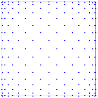
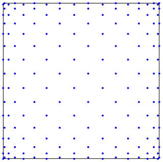
Figure 1: Left: 180 nodes for minimal cubature rule of degree 35 Right: 162 nodes for near-minimal cubature rule of degree 33

The Lagrange interpolation polynomials based on the nodes of these cubature rules were first studied in X96 . Let $L_{n}f(x,y)$ denote the Lagrange interpolation polynomial based on the nodes (10) for $n=2m$ and on (11) for $n=2m-1$, which belongs to the space $\Pi_{n}^{*}$ defined in (6). Using the Christoffel-Darboux formula in two variables, these interpolation polynomials can be given explicitly. Their convergence behavior is about optimal among all interpolation polynomials on the square. To be more precise, we introduce the following notation.

Let $\|\cdot\|_{p}$ denote the usual $L^{p}$ norm of the space $L^{p}(\Box,W_{0})$ for $1\leq p<\infty$, and define it as the uniform norm on the square $\Box$ when $p=\infty$. For $f\in C(\Box)$, let $E_{n}(f)_{\infty}$ be the error of best approximation by polynomials from $\Pi_{n}^{2}$ in the uniform norm; that is,

$$E_{n}(f)_{\infty}=\inf_{P\in\Pi_{n}^{2}}\|f-P\|_{\infty}.$$

Theorem 7

Let $f$ be a continuous function on $\Box$. Then

1. There is a constant $c>0$, independent of $n$ and $f$, such that

   $$\|f-L_{n}f\|_{p}\leq c\,E_{n}(f)_{\infty},\qquad 1\leq p<\infty;$$

2. The Lebesgue constant $\|L_{n}\|_{\infty}:=\sup_{\|f\|_{\infty}\neq 0}\|L_{n}f\|_{\infty}$ satisfies

   $$\|L_{n}\|_{\infty}=\mathcal{O}((\log n)^{2}),$$

   which is the optimal order among all projection operators from $C(\Omega)\mapsto\Pi_{n}^{*}$.

The first item was proved in X96 , which shows that $L_{n}f$ behaves like polynomials of best approximation in $L^{p}$ norm when $1\leq p<\infty$. The second one was proved more recently in BMV , which gives the upper bound of the Lebesgue constant; that this upper bound is optimal was established in SV . These results indicate that the set of points (10) is optimal for both numerical integration and interpolation. These interpolation polynomials were also considered in Ha1 , and further extended in Ha1A ; Ha2 , where points for other Chebyshev weights MP , including $(1-x^{2})^{\pm\frac{1}{2}}(1-y^{2})^{\mp\frac{1}{2}}$, are considered.

The interpolation polynomial $L_{n}f$ defined above is of degree $n$ and its set of interpolation points has the cardinality $\dim\Pi_{n-1}^{2}+\lfloor n/2\rfloor$ or one more. One could ask if it is possible to identify another set of points, say $X_{n}$, that has the cardinality $\dim\Pi_{n}^{2}$ and is just as good, which means that the interpolation polynomials based on $X_{n}$ should have the same convergence behavior as those in Theorem 7 and the cubature rule with $X_{n}$ as the set of nodes should be of the degree of precision $2n-1$. If such an $X_{n}$ exists, the points in $X_{n}$ need to be common zeros of polynomials of the form

$$\mathbb{P}_{n+1}+\Gamma_{1}\mathbb{P}_{n}+\Gamma_{2}\mathbb{P}_{n-1},$$

where $\Gamma_{1}$ and $\Gamma_{2}$ are matrices of sizes $(n+2)\times(n+1)$ and $(n+2)\times n$, respectively. For $W_{0}$, such a set indeed exists and known as the Padua points Pad1 ; Pad2 . One version of these points is

$$\begin{split}X_{n}:=&\left\{(\cos\tfrac{2i\pi}{n},\cos\tfrac{(2j-1)\pi}{n+1}),\quad 0\leq i\leq\lfloor\tfrac{n}{2}\rfloor\quad 1\leq j\leq\lfloor\tfrac{n}{2}\rfloor+1,\right.\\ &\left.(\cos\tfrac{(2i-1)\pi}{n},\cos\tfrac{(2j-2)\pi}{n+1}),\quad 1\leq i\leq\lfloor\tfrac{n}{2}\rfloor+1,\quad 1\leq j\leq\lfloor\tfrac{n}{2}\rfloor+2\right\},\end{split}$$ (12)

which are common zeros of polynomials $Q_{k}^{n+1}$, $0\leq k\leq n+1$, defined by

$$Q_{0}^{n+1}(x,y) =T_{n+1}(x)-T_{n-1}(x),$$ (13)

$$Q_{k}^{n+1}(x,y) =T_{n-k+1}(x)T_{k}(y)+T_{n-k+1}(y)T_{k-1}(x),\quad 1\leq k\leq n+1.$$ (14)

Theorem 8

For $n\in\mathbb{N}$, let $X_{n}$ be defined as in (12). Then $|X_{n}|=\dim\Pi_{n}^{2}$ and

1. There is a cubature rule of degree $2n-1$ with $X_{n}$ as its set of nodes.

2. There is a unique polynomial of degree $n$ that interpolates at the points in $X_{n}$, which enjoys the same convergence as that of $L_{n}f$ given in Theorem 7.

One interesting property of the Padua points is that they are self-intersection points of a Lissajous curve. For $X_{n}$ given in (12), the curve is given by $Q_{0}^{n+1}$ or, in parametric form,

$$(-\cos((n+1)t),-\cos(nt)),\qquad 0\leq t\leq(2n+1)\pi,$$

as shown in Figure 2. The generating curve offers a convenient tool for studying the interpolation polynomial based on Padua points.

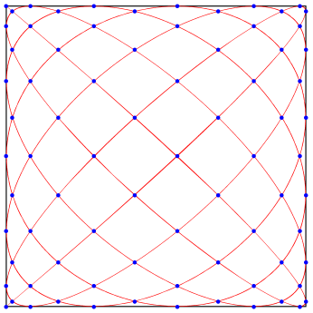
Figure 2: $78$ Padua points ($n=11$) and their generating curve

More generally, a Lissajous curve takes of the form $(\cos((n+p)t),\cos(nt))$ with positive integers $n$ and $p$ such that $n$ and $n+p$ are relatively prime. It is known F that such a curve has $(n-1)(n+p-1)/2$ self-intersection points inside $[-1,1]^{2}$. For $p\neq 1$, the number is not equal to the full dimension of $\Pi_{m}$ for any $m$ in general. Nonetheless, these points turn out to be good points for cubature rules and for polynomial interpolation, as shown in E1 ; E2 .

4 Results for a Family of Weight Functions

In this section we consider a family of weight functions that include the Chebyshev weight functions as special cases. Let $w$ be a weight function on the interval $[-1,1]$. For $\gamma>-1/2$, we define a weight function

$$\mathcal{W}_{\gamma}(x,y):=\, w(\cos(\theta-\phi))w(\cos(\theta+\phi))|x^{2}-y^{2}|(1-x^{2})^{\gamma}(1-y^{2})^{\gamma},$$

$$\qquad\hbox{where}\,\,x=\cos\theta,\,\,y=\cos\phi,\quad(x,y)\in[-1,1]^{2}.$$

When $w$ is the Jacobi weight function $w_{\alpha,\beta}(x):=(1-x)^{\alpha}(1+x)^{\beta}$, we denote the weight function $\mathcal{W}_{\gamma}$ by $W_{\alpha,\beta,\gamma}$. It is not difficult to verify that

$$W_{\alpha,\beta,\gamma}(x,y):=|x+y|^{2\alpha+1}|x-y|^{2\beta+1}(1-x^{2})^{\gamma}(1-y^{2})^{\gamma}.$$ (15)

In the special cases of $\alpha=\beta=-\frac{1}{2}$ and $\gamma=\pm\frac{1}{2}$, these are exactly the Chebyshev weight functions. It was proved recently in X12a ; X16 , rather surprisingly, that the results in the previous section can be extended to these weight functions. First, however, we describe a family of mutually orthogonal polynomials. To be more precise, we state this basis only for the weight function $W_{\alpha,\beta,\pm\frac{1}{2}}$.

For $\alpha,\beta>-1$, let $p_{n}^{(\alpha,\beta)}$ be the normalized Jacobi polynomial of degree $n$, so that $c_{\alpha,\beta}\int_{-1}^{1}|p_{n}^{(\alpha,\beta)}(x)|^{2}w_{\alpha,\beta}(x)dx=1$ and $p_{0}^{(\alpha,\beta)}(x)=1$. For $x=\cos\theta$ and $y=\cos\phi$, we define

$$P_{k,n}^{\alpha,\beta,-\frac{1}{2}}(2xy,x^{2}+y^{2}-1)$$

$$\,:=p_{n}^{(\alpha,\beta)}(\cos(\theta-\phi))p_{k}^{(\alpha,\beta)}(\cos(\theta+\phi))+p_{k}^{(\alpha,\beta)}(\cos(\theta-\phi))p_{n}^{(\alpha,\beta)}(\cos(\theta+\phi)),$$

$$P_{k,n}^{\alpha,\beta,\frac{1}{2}}(2xy,x^{2}+y^{2}-1)$$

$$\,:=\frac{p_{n+1}^{(\alpha,\beta)}(\cos(\theta-\phi))p_{k}^{(\alpha,\beta)}(\cos(\theta+\phi))-p_{k}^{(\alpha,\beta)}(\cos(\theta-\phi))p_{n+1}^{(\alpha,\beta)}(\cos(\theta+\phi))}{2\sin\theta\sin\phi}.$$

It turns out that $P_{k,n}^{\alpha,\beta,\pm\frac{1}{2}}(u,v)$ itself is a polynomial of degree $n$ in the variables $u$ and $v$, as can be seen by the elementary trigonometric identities

$$2xy=\cos(\theta-\phi)+\cos(\theta+\phi)\quad\hbox{and}\quad x^{2}+y^{2}-1=\cos(\theta-\phi)\cos(\theta+\phi),$$

and the fundamental theorem of symmetric polynomials. Furthermore, $P_{k,n}^{\alpha,\beta,\pm\frac{1}{2}}(u,v)$, first studied in K74a , are orthogonal polynomials with respect to a weight function on a domain bounded by a parabola and two straight lines and the weight function admit Gaussian cubature rules of all degrees SX . These polynomials are closely related to the orthogonal polynomials in $\mathcal{V}_{n}(W_{\alpha,\beta,-\frac{1}{2}})$, as shown in the following proposition established in X12b :

Proposition 9

Let $\alpha,\beta>-1$. A mutually orthogonal basis for $\mathcal{V}_{2m}(W_{\alpha,\beta,-\frac{1}{2}})$ is given by

$$\begin{split}{}_{1}Q_{k,2m}^{\alpha,\beta,\pm\frac{1}{2}}(x,y):=&P_{k,m}^{\alpha,\beta,\pm\frac{1}{2}}(2xy,x^{2}+y^{2}-1),\quad 0\leq k\leq m,\\ {}_{2}Q_{k,2m}^{\alpha,\beta,\pm\frac{1}{2}}(x,y):=&(x^{2}-y^{2})P_{k,m-1}^{\alpha+1,\beta+1,\pm\frac{1}{2}}(2xy,x^{2}+y^{2}-1),\quad 0\leq k\leq m-1,\end{split}$$ (16)

and a mutually orthogonal basis for $\mathcal{V}_{2m+1}(W_{\alpha,\beta,\pm\frac{1}{2}})$ is given by

$$\begin{split}{}_{1}Q_{k,2m+1}^{\alpha,\beta,\pm\frac{1}{2}}(x,y):=&(x+y)P_{k,m}^{\alpha,\beta+1,\pm\frac{1}{2}}(2xy,x^{2}+y^{2}-1),\quad 0\leq k\leq m,\\ {}_{2}Q_{k,2m+1}^{\alpha,\beta,\pm\frac{1}{2}}(x,y):=&(x-y)P_{k,m-1}^{\alpha+1,\beta,\pm\frac{1}{2}}(2xy,x^{2}+y^{2}-1),\quad 0\leq k\leq m.\end{split}$$ (17)

The orthogonal polynomials in (16) of degree $2n$ are symmetric polynomials in $x$ and $y$, and they are invariant under $(x,y)\mapsto(-x,-y)$. Notice, however, that the product Chebyshev polynomials do not possess such symmetries, even though $W_{-\frac{1}{2},-\frac{1}{2},\pm\frac{1}{2}}$ are the Chebyshev weight functions.

We now return to cubature rules and interpolation and state the following theorem.

Theorem 10

The minimal cubature rules of degree $2n-1$ that attain the lower bound (5) exist for the weight function $\mathcal{W}_{\pm\frac{1}{2}}$ when $n=2m$. Moreover, the same holds for the weight function $W_{\alpha,\beta,\pm\frac{1}{2}}$ when $n=2m+1$.

The orthogonal polynomials whose common zeros are nodes of these cubature rules, as described in Theorem 4, can be identified explicitly. Let us consider only $W_{\alpha,\beta,-\frac{1}{2}}$. For $n=2m$, these polynomials can be chosen as ${}_{1}Q_{k,2m}^{\alpha,\beta,-\frac{1}{2}}$, $0\leq k\leq m$, in (16). For $n=2m+1$, they can be chosen as ${}_{2}Q_{k,2m+1}^{\alpha,\beta,-\frac{1}{2}}$, $0\leq k\leq m$, in (17), together with one more polynomial

$$q_{m}(x,y)=(x+y) \left[p_{m}^{(\alpha,\beta+1)}(\cos(\theta-\phi))p_{m}^{(\alpha+1,\beta)}(\cos(\theta+\phi))\right.$$

$$\left.+p_{m}^{(\alpha,\beta+1)}(\cos(\theta+\phi))p_{m}^{(\alpha+1,\beta)}(\cos(\theta-\phi))\right]$$

in $\mathcal{V}_{2m+1}(W_{\alpha,\beta,-\frac{1}{2}})$, as shown in X16 . For $n=2m$, the nodes of the minimal cubature rules for $W_{\alpha,\beta,-\frac{1}{2}}$ are not as explicit as those for $n=2m$. For interpolation, it is often easier to work with the near minimal cubature rule of degree $2n-1$ when $n=2m+1$, whose number of nodes is just one more than the minimal number $N_{\min}$ in (5). The nodes of the these near minimal rules are common zeros of ${}_{2}Q_{k,2m+1}^{\alpha,\beta,-\frac{1}{2}}$, $0\leq k\leq m$, and a quasi-orthogonal polynomial of the form ${}_{1}Q_{k,2m+2}^{\alpha,\beta,-\frac{1}{2}}-a_{k,m}{}_{1}Q_{k,2m}^{\alpha,\beta,-\frac{1}{2}}$, where $a_{k,m}$ are specific constants ((X16, , Theorem 3.5)).

The nodes of these cubature rules can be specified. For $\alpha,\beta>-1$ and $1\leq k\leq m$, let $\cos\theta_{k,m}^{\alpha,\beta}$ be the zeros of the Jacobi polynomial $P_{m}^{\alpha,\beta}$ so that

$$0<\theta_{1,m}^{\alpha,\beta}<\ldots<\theta_{m,m}^{\alpha,\beta}<\pi,$$

and we also define $\theta_{0,m}^{\alpha,\beta}=0$. We further define

$$s_{j,k}^{\alpha,\beta}:=\cos\tfrac{\theta_{j,n}-\theta_{k,n}}{2}\quad\hbox{and}\quad t_{j,k}^{\alpha,\beta}:=\cos\tfrac{\theta_{j,n}+\theta_{k,n}}{2},\qquad\hbox{where}\quad\theta_{k,n}=\theta_{k,n}^{\alpha,\beta}.$$

For $n=2m$, the nodes of the minimal cubature rule of degree $2n-1$ consist of

$$X_{2m}^{\alpha,\beta}:=\{(s_{j,k}^{\alpha,\beta},t_{j,k}^{\alpha,\beta}),(t_{j,k}^{\alpha,\beta},s_{j,k}^{\alpha,\beta}),(-s_{j,k}^{\alpha,\beta},-t_{j,k}^{\alpha,\beta}),(-t_{j,k}^{\alpha,\beta},-s_{j,k}^{\alpha,\beta}):1\leq j\leq k\leq m\}.$$

For $n=2m+1$, the nodes of the near minimal cubature rule of degree $2n-1$ consist of

$$X_{2m+1}^{\alpha,\beta}:=\{(s_{j,k}^{\alpha+1,\beta},t_{j,k}^{\alpha+1,\beta}), (t_{j,k}^{\alpha+1,\beta},s_{j,k}^{\alpha+1,\beta}),(-s_{j,k}^{\alpha+1,\beta},-t_{j,k}^{\alpha+1,\beta}),$$

$$(-t_{j,k}^{\alpha+1,\beta},-s_{j,k}^{\alpha+1,\beta}):0\leq j\leq k\leq m\}.$$

The weight function $W_{\alpha,\beta,-\frac{1}{2}}$ has a singularity at the diagonal $y=x$ of the square when $\alpha\neq-\frac{1}{2}$, or at the diagonal $y=-x$ of the square when $\beta\neq-\frac{1}{2}$, or at both diagonals when neither $\alpha$ nor $\beta$ equal to $-\frac{1}{2}$. This is reflected in the distribution of the nodes, which are propelled away from these diagonals. Furthermore, for a fixed $m$, the points in $X_{2m}$ and $X_{2m+1}$ will be propelled further away for increasing values of $\alpha$ and/or $\beta$. In Figure 3 we depict the nodes of the minimal cubature rules of degree 31 for $W_{\frac{1}{2},\frac{1}{2},-\frac{1}{2}}$, which has singularity on both diagonals, and for $W_{\frac{1}{2},-\frac{1}{2},-\frac{1}{2}}$, which has singularity at the diagonal $y=x$. Writing explicitly, these weight functions are

$$W_{\frac{1}{2},\frac{1}{2},-\frac{1}{2}}(x,y)=\frac{(x-y)^{2}(x+y)^{2}}{\sqrt{1-x^{2}}\sqrt{1-y^{2}}}\quad\hbox{and}\quad W_{\frac{1}{2},-\frac{1}{2},-\frac{1}{2}}(x,y)=\frac{(x-y)^{2}}{\sqrt{1-x^{2}}\sqrt{1-y^{2}}}.$$

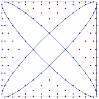
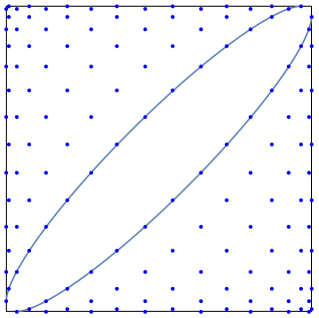
Figure 3: 144 nodes for minimal cubature rule of degree 31 for the weight functions $W_{\frac{1}{2},\frac{1}{2},-\frac{1}{2}}$ (left) and $W_{\frac{1}{2},-\frac{1}{2},-\frac{1}{2}}$ (right)

We also depicted the curves that bound the region that does not contain any nodes, which are given in explicit parametric formulas in (X16, , Proposition 3.6). The region without nodes increases in size when $\alpha$ and/or $\beta$ increase for a fixed $m$, but they are getting smaller when $m$ increases while $\alpha$ and $\beta$ are fixed. These figures can be compared to those in Figure 1 for the case $\alpha=\beta=-\frac{1}{2}$, where the obvious symmetry in $X_{n}^{\alpha,\beta}$ is not evident.

Let $L_{n}^{\alpha,\beta}f$ be the interpolation polynomial based on $X_{2m}^{\alpha,\beta}$ when $n=2m$ and on $X_{2m+1}^{\alpha,\beta}$ when $n=2m+1$, as defined in (7). The asymptotics of the Lebesgue constants for these interpolation polynomials can be determined X12a ; X16 .

Theorem 11

Let $\alpha,\beta\geq-1/2$. The Lebesgue constant of the Lagrange interpolation polynomial $\mathcal{L}_{n}^{\alpha,\beta}f$ satisfies

$$\|\mathcal{L}_{n}^{\alpha,\beta}\|_{\infty}=\mathcal{O}(1)\begin{cases}n^{2\max\{\alpha,\beta\}+1},&\max\{\alpha,\beta\}>-1/2,\\ (\log n)^{2},&\max\{\alpha,\beta\}=-1/2.\end{cases}$$ (18)

It should be mentioned that an explicit formula for the kernel $K_{n}^{*}$ in (8) is known, so that the interpolation polynomials $L_{n}^{\alpha,\beta}f$ can be written down in closed form without solving a large linear system of equations.

5 Minimal Cubature Rules for Constant Weight

The weight functions in the previous two sections contain the Chebyshev weight functions but do not include the weight functions $(1-x^{2})^{\lambda}(1-y^{2})^{\lambda}$ for $\lambda\neq\pm\frac{1}{2}$. In particular, it does not include the constant weight function $W(x,y)=1$.

For these weight functions, it is possible to establish their existence when $n$ is small. In this section we discuss how these formulas can be constructed. For cubature rules of degree $2n-2$, we consider the Gaussian cubature rules described in the item 2 of Theorem 2. For cubature rules of degree $2n-1$, we consider minimal cubature rules that attain the lower bound (5). Both these cases can be characterized by non-linear system of equations, which may or may not have solutions. We shall describe these equations and solve them for the constant weight function for small $n$. The known cases for these cubature rules are listed in Cools1 ; Cools2 .

Throughout the rest of this section, we shall assume that $W(x,y)=1$. Let $\mathcal{V}_{n}$ be the space of orthogonal polynomials of degree $n$ with respect to the inner product $\langle f,g\rangle=\frac{1}{2}\int_{\Box}f(x,y)g(x,y)dxdy$. Then an orthonormal basis of $\mathcal{V}_{n}$ is given by

$$P_{k}^{n}(x,y)=\widehat{P}_{n-k}(x)\widehat{P}_{k}(y),\qquad 0\leq k\leq n,$$

where $\widehat{P}_{n}=\sqrt{2n+1}P_{n}$ and $P_{n}$ is the classical Legendre polynomial of degree $n$. In this case, the coefficients $B_{n,i}$ in the three-term relations (3) are zero and the three-term relations take the form

$$x\mathbb{P}_{n}(x,y) =A_{n,1}\mathbb{P}_{n+1}(x,y)+A_{n-1,1}^{\mathsf{t}}\mathbb{P}_{n-1}(x,y),$$

$$y\mathbb{P}_{n}(x,y) =A_{n,2}\mathbb{P}_{n+1}(x,y)+A_{n-1,2}^{\mathsf{t}}\mathbb{P}_{n-1}(x,y),$$

where $\mathbb{P}_{n}=(P_{0}^{n},\ldots,P_{n}^{n})^{\mathsf{t}}$, $A_{n,1}$ and $A_{n,2}$ are given by

$$A_{n,1}=\left[\begin{matrix}a_{n}&&\bigcirc&0\cr&\ddots&&\vdots\cr\bigcirc&&a_{0}&0\end{matrix}\right]\quad\hbox{and}\quad A_{n,2}=\left[\begin{matrix}0&a_{0}&&\bigcirc\cr\vdots&&\ddots&\cr 0&\bigcirc&&a_{n}\end{matrix}\right],$$

in which

$$a_{k}:=\frac{k+1}{\sqrt{(2k+1)(2k+3)}},\qquad k=0,1,2,....$$

5.1 Minimal cubature rules of degree $2n-2$

By Theorem 2, the nodes of a Gaussian cubature rule of degree $2n-2$, if it exists, are common zeros of $\mathbb{P}_{n}+\Gamma_{n}\mathbb{P}_{n-1}$ for some matrix $\Gamma_{n}$ of size $(n+1)\times n$. The latter is characterized in the following theorem X94a .

Theorem 12

The polynomials in $\mathbb{P}_{n}+\Gamma_{n}\mathbb{P}_{n-1}$ have $n(n+1)/2$ real, distinct zeros if, and only if, $\Gamma_{n}$ satisfies

$$A_{n-1,1}\Gamma_{n}=\Gamma_{n}^{\mathsf{t}}A_{n-1,1}^{\mathsf{t}},\quad \quad A_{n-1,2}\Gamma_{n}=\Gamma_{n}^{\mathsf{t}}A_{n-1,2}^{\mathsf{t}},$$ (19)

$$\Gamma_{n}^{\mathsf{t}}(A_{n-1,1}^{\mathsf{t}}A_{n-1,2}-A_{n-1,2}^{\mathsf{t}}A_{n-1,1})\Gamma_{n} =(A_{n-1,1}A_{n-1,2}^{\mathsf{t}}-A_{n-1,2}A_{n-1,1}^{\mathsf{t}}).$$ (20)

The equations in (19) imply that $\Gamma_{n}$ can be written in terms of a Hankel matrix $H_{n}=(h_{i+j})$ of size $(n+1)\times n$,

$$\Gamma=G_{n}H_{n}G_{n-1}^{\mathsf{t}},\quad\hbox{where}\quad G_{n}=\mathrm{diag}\{g_{n,0},g_{n-1,1},\ldots,g_{1,n-1},g_{0,n}\}$$ (21)

with

$$g_{n-k,k}=\gamma_{n-k}\gamma_{k}\quad\hbox{and}\quad\gamma_{k}=\frac{(2k)!\sqrt{2k+1}}{2^{k}k!^{2}}.$$

Thus, solving the system of equations in Theorem 12 is equivalent to solving (20) for the Hankel matrix $H_{n}$, which is a nonlinear system of equations and its solution may not exist. Since the matrices in both sides of (20) are skew symmetric, the nonlinear system consists of $n(n-1)/2$ equations and $2n$ variables. The number of variables is equal to the number of equations when $n=5$.

We found the solution when $n=3,4,5$, which gives Gaussian cubature rules of degree $4,6,8$. These cases are known in the literature, see the list in Cools1 . In the case $n=3$ and $n=4$, we were able to solve the system analytically instead of numerically. For $n=3$, the matrix $H_{3}$ takes the form

$$H_{3}=\frac{4}{27\sqrt{7}}\left[\begin{matrix}-\frac{11}{25}&0&1\\ 0&1&0\\ 1&0&\frac{2}{5}\\ 0&\frac{2}{5}&0\end{matrix}\right].$$

The case $H_{4}$ is too cumbersome to write down. In the case $n=5$, the system is solved numerically, which has multiple solutions but essentially one up to symmetry. This solution, however, has one common zero (or node of the Gaussian cubature rule of degree 8) that lies outside of the square, which agrees with the list in Cools2 .

Solving the system for $n>5$ numerically yields no solution. It is tempting to proclaim that the Gaussian cubature rules of degree $2n-2$ for the constant weight function on the square do not exist for $n\geq 6$, but a proof is still needed.

5.2 Minimal cubature rules of degree $2n-1$

Here we consider minimal cubature rules of degree $2n-1$ that attain the lower bound (5). By Theorem 4, the nodes of such a cubature rule are common zeros of $(n+1)-\lfloor n/2\rfloor$ many orthogonal polynomials of degree $n$, which can be written as the elements of $U^{\mathsf{t}}\mathbb{P}_{n}$, where $U$ is a matrix of size $(n+1)\times(n+1-\lfloor n/2\rfloor)$ and $U$ has full rank.

Theorem 13

There exist $(n+1)-\lfloor n/2\rfloor$ many orthogonal polynomials of degree $n$, written as $U^{\mathsf{t}}\mathbb{P}_{n}$, that have $n(n+1)+\lfloor\frac{n}{2}\rfloor$ real, distinct common zeros if, and only if, $U$ satisfies $U^{\mathsf{t}}V=0$ for a matrix $V$ of size $(n+1)\times\lfloor\frac{n}{2}\rfloor$ that satisfies

$$A_{n-1,1}(VV^{\mathsf{t}}-I)A_{n-1,2}^{\mathsf{t}}=A_{n-1,2}(VV^{\mathsf{t}}-I)A_{n-1,2}^{\mathsf{t}},$$ (22)

$$VV^{\mathsf{t}}(A_{n-1,1}^{\mathsf{t}}A_{n-1,2}-A_{n-1,2}^{\mathsf{t}}A_{n-1,1})VV^{\mathsf{t}}=0,$$ (23)

where $I$ denotes the identity matrix.

The equation (22) implies that the matrix $VV^{\mathsf{t}}$ can be written in terms of a Hankel matrix $H_{n}$ of size $(n+1)\times(n+1)$,

$$VV^{\mathsf{t}}=I+G_{n}H_{n}G_{n}^{\mathsf{t}}:=W,$$

where $G_{n}$ is defined as in (21). Thus, to find the matrix $V$ we need to solve (23) for $H_{n}$ and make sure that the matrix $W$ is nonnegative definite and has rank $\lfloor\frac{n}{2}\rfloor$, so that it can be factored as $VV^{\mathsf{t}}$. The non-linear system (23) consists of $n(n+1)/2$ equations and has $2n+1$ variables, which may not have a solution.

Comparing with the Gaussian cubature rules of even degree in the previous subsection, however, the situation here is more complicated. We not only need to solve (23), similar to solving (20), for $H_{n}$, we also have to make sure that the resulting $W$ is non-negative definite and has rank $\lfloor\frac{n}{2}\rfloor$, which poses an additional constraint that is not so easy to verify.

We found the solutions when $n=3,4,5$ and $6$, which gives minimal cubature rules of degree $5,7,9,11$. These cases are all known in the literature, see the list in Cools1 and the references therein. In the case of $n=4$, there are multiple solutions; for example, one solution has all 12 points inside the square and another one has 2 points outside. In the case $n=3,4,5$, we were able to solve the system analytically instead of numerically. We give Hankel matrices $H_{n}$ for those cases that have all nodes of the minimal cubature rules inside the square:

$$H_{3}=\frac{4}{135}\left[\begin{matrix}-\frac{8}{35}&0&1&0\\ 0&1&0&0\\ 1&0&0&0\\ 0&0&0&\frac{4}{35}\end{matrix}\right],\qquad H_{4}=\frac{44}{14385}\left[\begin{matrix}\frac{94}{231}&1&1&1&-\frac{82}{55}\\ 1&1&1&-\frac{82}{55}&1\\ 1&1&-\frac{82}{55}&1&1\\ 1&-\frac{82}{55}&1&1&1\\ -\frac{82}{55}&1&1&1&\frac{94}{231}\end{matrix}\right],$$

and

$$H_{5}=\frac{96}{77875}\left[\begin{matrix}\frac{1151}{2079}&\frac{10\sqrt{86}}{189}&-\frac{31}{86}&-\frac{1}{9}\sqrt{\frac{43}{2}}&1&0\\ \frac{10\sqrt{86}}{189}&-\frac{31}{86}&-\frac{1}{9}\sqrt{\frac{43}{2}}&1&0&1\\ -\frac{31}{86}&-\frac{1}{9}\sqrt{\frac{43}{2}}&1&0&1&\frac{1}{9}\sqrt{\frac{43}{2}}\\ -\frac{1}{9}\sqrt{\frac{43}{2}}&1&0&1&\frac{1}{9}\sqrt{\frac{43}{2}}&-\frac{31}{86}\\ \\ 1&0&1&\frac{1}{9}\sqrt{\frac{43}{2}}&-\frac{31}{86}&-\frac{10\sqrt{86}}{189}\\ 0&1&\frac{1}{9}\sqrt{\frac{43}{2}}&-\frac{31}{86}&-\frac{10\sqrt{86}}{189}&\frac{1151}{2079}\end{matrix}\right].$$

Once $H_{n}$ is found, it is easy to verify that $W$ satisfies the desired rank condition and is non-negative definite. We can then find $U$, or the set of orthogonal polynomials, and then find common zeros. For example, when $n=5$, we have $4$ orthogonal polynomials of degree $5$ given by

$$Q_{1}(x,y)= \frac{10\sqrt{86}}{189}P_{0}^{5}(x,y)+\frac{1081\sqrt{11}}{2835\sqrt{3}}P_{1}^{5}(x,y)+P_{5}^{5}(x,y),$$

$$Q_{2}(x,y)= \frac{205}{21\sqrt{33}}P_{0}^{5}(x,y)+\frac{10\sqrt{86}}{189}P_{1}^{5}(x,y)+P_{4}^{5}(x,y),$$

$$Q_{3}(x,y)= -\frac{5\sqrt{438}}{27\sqrt{77}}P_{0}^{5}(x,y)+\frac{62\sqrt{5}}{81\sqrt{21}}P_{1}^{5}(x,y)+P_{3}^{5}(x,y),$$

$$Q_{4}(x,y)= -\frac{10\sqrt{5}}{3\sqrt{77}}P_{0}^{5}(x,y)-\frac{\sqrt{430}}{9\sqrt{21}}P_{1}^{5}(x,y)+P_{2}^{5}(x,y),$$

which has 17 real common zeros inside the square. Only numerical results are known for the case $n=6$. We also tried the case $n=7$, but found no solution numerically.

Acknowledgements The author thanks two anonymous referees for their careful reading and corrections.

References

- (1) Bojanov, B., Petrova, G.: On minimal cubature formulae for product weight function. J. Comput. Appl. Math. 85, 113–121 (1997)
- (2) Bos, L., Caliari, M., De Marchi, S., Vianello, M., Xu, Y.: Bivariate Lagrange interpolation at the Padua points: the generating curve approach. J. Approx. Theory 143, 15–25 (2006)
- (3) Bos, L., De Marchi, S., Vianello, M.: On the Lebesgue constant for the Xu interpolation formula. J. Approx. Theory 141, 134–141 (2006)
- (4) Bos, L., De Marchi, S., Vianello, M., Xu, Y.: Bivariate Lagrange interpolation at the Padua points: The ideal theory approach. Numer. Math. 108, 43–57 (2007)
- (5) Cools, R.: Monomial cubature rules since “Stroud”: a compilation – part 2. J. Comput. Appl. Math. 112, 21–27 (1999)
- (6) Cools, R., Rabinowitz, P.: Monomial cubature rules since “Stroud”: a compilation. J. Comput. Appl. Math. 48, 309–326 (1993)
- (7) Dick, J., Kuo, F., Sloan, I.: High-dimensional integration: the quasi-Monte Carlo way. Acta Numer. 22, 133–288 (2013)
- (8) Dunkl, C. F., Xu, Y.: Orthogonal Polynomials of Several Variables, Encyclopedia of Mathematics and its Applications 155, Cambridge University Press, Cambridge (2014)
- (9) Erb, W.: Bivariate Lagrange interpolation at the node points of Lissajous curves – the degenerate case. Appl. Math. Comput. 289, 409–425 (2016)
- (10) Erb, W., Kaethner, C., Ahlborg, M., Buzug, T. M.: Bivariate Lagrange interpolation at the node points of non–degenerate Lissajous curves. Numer. Math. 133, 685–705 (2016)
- (11) Fischer, G.: Plane algebraic curves, translated by Leslie Kay. American Mathematical Society (AMS), Providence, RI (2001)
- (12) Harris, L.: Bivariate Lagrange interpolation at the Chebyshev nodes. Proc. Amer. Math. Soc. 138, 4447–4453 (2010)
- (13) Harris, L.: Bivariate polynomial interpolation at the Geronimus nodes, Complex analysis and dynamical systems V, 135–147, Contemp. Math., 591, Israel Math. Conf. Proc., Amer. Math. Soc., Providence, RI (2013)
- (14) Harris, L.: Lagrange polynomials, reproducing kernels and cubature in two dimensions. J. Approx. Theory, 195, 43–56 (2015)
- (15) Koornwinder, T. H.: Orthogonal polynomials in two variables which are eigenfunctions of two algebraically independent partial differential operators, I, II. Proc. Kon. Akad. v. Wet., Amsterdam 36, 48–66 (1974)
- (16) Li, H., Sun, J., Xu, Y.: Cubature formula and interpolation on the cubic domain. Numer. Math. Theory Methods Appl. 2, 119–152 (2009)
- (17) Möller, H.: Kubaturformeln mit minimaler Knotenzahl. Numer. Math. 25, 185–200 (1976)
- (18) Morrow, C. R., Patterson, T. N. L.: Construction of algebraic cubature rules using polynomial ideal theory. SIAM J. Numer. Anal. 15, 953–976 (1978)
- (19) Mysovskikh, I. P.: Numerical characteristics of orthogonal polynomials in two variables. Vestnik Leningrad Univ. Math. 3, 323–332 (1976)
- (20) Mysovskikh, I. P.: Interpolatory cubature formulas. Nauka, Moscow (1981)
- (21) Schmid, H.: On cubature formulae with a minimal number of knots. Numer. Math. 31, 282–297 (1978)
- (22) Schmid, H., Xu, Y.: On bivariate Gaussian cubature formula. Proc. Amer. Math. Soc. 122, 833–842 (1994)
- (23) Stroud, A. H.: Approximate calculation of multiple integrals. Prentice-Hall, Inc., Englewood Cliffs, N.J. (1971)
- (24) Szili, L., Vértesi, P.: On multivariate projection operators. J. Approx. Theory 159, 154–164 (2009)
- (25) Xu, Y.: Gaussian cubature and bivariable polynomial interpolation. Math. Comput. 59, 547–555 (1992)
- (26) Xu, Y.: Common zeros of polynomials in several variables and higher dimensional quadrature, Pitman Research Notes in Mathematics Series, Longman, Essex (1994)
- (27) Xu, Y.: On zeros of multivariate quasi-orthogonal polynomials and Gaussian cubature formulae. SIAM J. Math. Anal. 25, 991–1001 (1994)
- (28) Xu, Y.: Lagrange interpolation on Chebyshev points of two variables. J. Approx. Theory 87, 220–238 (1996)
- (29) Xu, Y.: Minimal Cubature rules and polynomial interpolation in two variables. J. Approx. Theory 164, 6–30 (2012).
- (30) Xu, Y.: Orthogonal polynomials and expansions for a family of weight functions in two variables. Constr. Approx. 36, 161–190 (2012).
- (31) Xu, Y.: Minimal Cubature rules and polynomial interpolation in two variables, II. J. Approx. Theory 214, 49–68 (2017)