MILP and Max-Clique based heuristics for the Eternity II puzzle

Abstract

The present paper considers a hybrid local search approach to the Eternity II puzzle and to unsigned, rectangular, edge matching puzzles in general. Both an original mixed-integer linear programming (MILP) formulation and a novel Max-Clique formulation are presented for this NP-hard problem. Although the presented formulations remain computationally intractable for medium and large sized instances, they can serve as the basis for developing heuristic decompositions and very large scale neighbourhoods. As a side product of the Max-Clique formulation, new hard-to-solve instances are published for the academic research community. Two reasonably well performing MILP-based constructive methods are presented and used for determining the initial solution of a multi-neighbourhood local search approach. Experimental results confirm that this local search can further improve the results obtained by the constructive heuristics and is quite competitive with the state of the art procedures.

1 Introduction

The Eternity II puzzle (EII) is a commercial edge matching puzzle in which 256 square tiles with four coloured edges must be arranged on a $16\times 16$ grid such that all tile edges are matched. In addition, a complete solution requires that the ‘grey’ patterns, which appear only on a subset of the tiles, should be matched to the outer edges of the grid. An illustration of a complete solution for a small size puzzle, $5\times 5$, is provided in Figure 1.

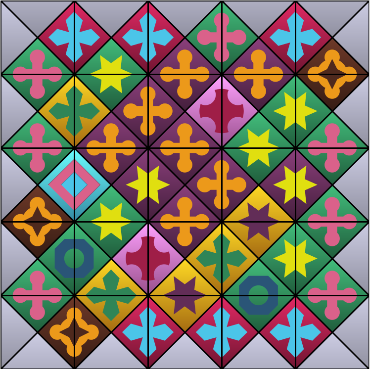
Figure 1: Solution to an Eternity II-like edge matching puzzle of size $5\times 5$ (Image generated with the Eternity II editor, http://sourceforge.net/projects/eternityii/, accessed on 24 January 2014)

The EII puzzle was created by Christopher Monckton and released by the toy distributor Tomy UK Ltd. in July 2007. Along with the puzzle release, a large cash prize of 2 million USD was announced to be awarded to the first person who could solve the puzzle. As can be expected, this competition attracted considerable attention. Many efforts were made to tackle this challenging problem, yielding interesting approaches and results. However, no complete solution has ever been generated. Meanwhile, the final scrutiny date for the cash price, 31 December 2010, has passed, leaving the large money prize unclaimed.

The EII puzzle belongs to the more general class of Edge Matching Puzzles, which have been shown to be NP-complete [5]. Many approaches to Edge Matching Puzzles are now available in the literature. Constraint programming approaches [2, 11] have been developed, in addition to metaheuristics [4, 11, 13], backtracking [12] and evolutionary methods [10]. Other methods translate the problem into a SAT formulation and then solve it with SAT solvers [1, 7]. An extensive literature overview on the topic is provided in [14], while [8] provides a survey on the complexity of other puzzles.

The present paper introduces a novel Mixed-Integer Linear Programming (MILP) model and a novel Max-Clique based formulation for EII-like puzzles of size $n\times n$. Both formulations serve as components of heuristic decompositions used in a multi-neighbourhood local search approach. The remainder of the paper is structured as follows. Section 2 presents the MILP and Max-Clique formulations. In Section 3, several hybrid heuristic approaches are introduced. Computational results are presented in Section 4. Final conclusions are drawn in Section 5.

2 Problem formulations

2.1 Mixed integer linear programming formulation

A novel mixed-integer linear programming model was developed for the EII puzzle problem. The following notation will be used. The puzzle consists of an $n\times n$ square onto which $n^{2}$ tiles need to be placed. The index $t=1\ldots n^{2}$ is used to refer to tiles. The indices $r=1\ldots n$, $c=1\ldots n$ denote the rows, resp. columns, of the puzzle board. The index $\alpha=0\ldots 3$ refers to the rotation of the tile, i.e. $\alpha=0$ means not rotated, $\alpha=1$ means rotated clockwise over $90^{\circ}$, etc. The coefficient $CT_{t,\alpha,l}$ (resp. $CB$, $CL$, $CR$) is equal to $1$ if tile $t$ has colour $l$ at its top (resp. bottom, left, right) position when rotated by $\alpha$.

The decision variables of the MILP model are defined as follows:

$$x_{t,r,c,\alpha}= \begin{cases}1&\textrm{if tile $t$ is placed in row $r$, column $c$ with rotation $\alpha$},\\ 0&\textrm{otherwise}.\end{cases}$$

$$h_{r,c}= \begin{cases}1&\textrm{if the right edge of position $(r,c)$ is \emph{unmatched}},\\ 0&\textrm{otherwise}.\end{cases}$$

$$v_{r,c}= \begin{cases}1&\textrm{if the bottom edge of position $(r,c)$ is \emph{unmatched}},\\ 0&\textrm{otherwise}.\end{cases}$$

The model is then defined as follows:

$$\textrm{Min}\ \sum_{r=1}^{n}\sum_{c=1}^{n-1}h_{r,c}+\sum_{r=1}^{n-1}\sum_{c=1}^{n}v_{r,c}$$ (1)

$$s.t.$$

$$\sum_{r=1}^{n}\sum_{c=1}^{n}\sum_{\alpha=0}^{3}x_{t,r,c,\alpha}=1\quad\forall t=1,\ldots,n^{2}$$ (2)

$$\sum_{t=1}^{n^{2}}\sum_{\alpha=0}^{3}x_{t,r,c,\alpha}=1\quad\forall r=1,\ldots,n,\;c=1,\ldots,n$$ (3)

$$\sum_{t=1}^{n^{2}}{\sum_{\alpha=0}^{3}{CR_{t,\alpha,l}x_{t,r,c,\alpha}}}-\sum_{t=1}^{n^{2}}{\sum_{\alpha=0}^{3}{CL_{t,\alpha,l}x_{t,r,c+1,\alpha}}}\leq h_{r,c}$$

$$\quad\forall r=1,\ldots,n,\;c=1,\ldots,n-1,\;l=1,\ldots,L$$ (4)

$$- \sum_{t=1}^{n^{2}}{\sum_{\alpha=0}^{3}{CR_{t,\alpha,l}x_{t,r,c,\alpha}}}+\sum_{t=1}^{n^{2}}{\sum_{\alpha=0}^{3}{CL_{t,\alpha,l}x_{t,r,c+1,\alpha}}}\leq h_{r,c}$$

$$\quad\forall r=1,\ldots,n,\;c=1,\ldots,n-1,\;l=1,\ldots,L$$ (5)

$$\sum_{t=1}^{n^{2}}{\sum_{\alpha=0}^{3}{CB_{t,\alpha,l}x_{t,r,c,\alpha}}}-\sum_{t=1}^{n^{2}}{\sum_{\alpha=0}^{3}{CT_{t,\alpha,l}x_{t,r+1,c,\alpha}}}\leq v_{r,c}$$

$$\quad\forall r=1,\ldots,n-1,\;c=1,\ldots,n,\;l=1,\ldots,L$$ (6)

$$- \sum_{t=1}^{n^{2}}{\sum_{\alpha=0}^{3}{CB_{t,\alpha,l}x_{t,r,c,\alpha}}}+\sum_{t=1}^{n^{2}}{\sum_{\alpha=0}^{3}{CT_{t,\alpha,l}x_{t,r+1,c,\alpha}}}\leq v_{r,c}$$

$$\quad\forall r=1,\ldots,n-1,\;c=1,\ldots,n,\;l=1,\ldots,L$$ (7)

$$\sum_{t=1}^{n^{2}}{\sum_{\alpha=0}^{3}{CT_{t,\alpha,0}\cdot x_{t,0,c,\alpha}}}=1\quad\forall c=1,\ldots,n$$ (8)

$$\sum_{t=1}^{n^{2}}{\sum_{\alpha=0}^{3}{CB_{t,\alpha,0}\cdot x_{t,n-1,c,\alpha}}}=1\quad\forall c=1,\ldots,n$$ (9)

$$\sum_{t=1}^{n^{2}}{\sum_{\alpha=0}^{3}{CL_{t,\alpha,0}\cdot x_{t,r,0,\alpha}}}=1\quad\forall r=1,\ldots,n$$ (10)

$$\sum_{t=1}^{n^{2}}{\sum_{\alpha=0}^{3}{CR_{t,\alpha,0}\cdot x_{t,r,n-1,\alpha}}}=1\quad\forall r=1,\ldots,n$$ (11)

$$x_{t,r,c,\alpha}\in\{0,1\}$$

$$\forall t=1,\ldots,n^{2},\;r=1,\ldots,n,\;c=1,\ldots,n,\;\alpha=0,\ldots,3$$ (12)

$$0\leq h_{r,c}\leq 1\quad\forall r=1,\ldots,n,\;c=1,\ldots,n-1$$ (13)

$$0\leq v_{r,c}\leq 1\quad\forall r=1,\ldots,n-1,\;c=1,\ldots,n$$ (14)

The objective function (Expression 1) minimises the number of unmatched edges in the inner region of the puzzle. Constraints (2) indicate that each tile must be assigned to exactly one position, with one rotation. Constraints (3) require that exactly one tile must be assigned to a position. The edge constraints (4) and (5) force the $h_{r,c}$ variables to take on the value 1 if the tiles on positions $(r,c)$ and $(r,c+1)$ are unmatched. Similarly, constraints (6) and (7) do the same for the vertical edge variables $v_{r,c}$. Finally, constraints (8) - (11) ensure that the border edges are matched to the gray frame (colour $l=0$).

We point out that constraining the objective function to zero (i.e. no unmatched edges allowed), turns the model into a feasibility problem where every feasible solution is also optimal. However, preliminary testing showed that the latter model is only relevant for very small size problem instances. If the MILP solver needs to be stopped prematurely on the feasibility model, no solution is returned.

2.2 Clique formulation

The EII puzzle itself is a decision problem and can be modelled as (i.e. it reduces to) the well known decision version of the clique problem [3] as follows. Given a parameter $k$ and an undirected graph $G=(V,E)$, the clique problem calls for finding a subset of pairwise adjacent nodes, called a clique, with a cardinality greater than or equal to $k$. Let the nodes of the graph correspond to variables $x_{t,r,c,\alpha}$ from the formulation introduced in Section 2.1. Each node thus represents a tile in a given position on the puzzle and with a given rotation $\alpha$. The nodes are connected $\mathrm{iff}$ there is no conflict between the nodes in the puzzle. Possible causes of conflicts are:

• unmatching colors for adjacent positions

• same tile assigned to different positions

• same tile assigned to the same position with different rotations

• different tiles assigned to the same position.

The objective is to find a clique of size $n^{2}$, where $n$ is the size of the puzzle.

2.3 Comparison of the MILP model and the Clique model

The applicability of the MILP model and the Clique model is investigated in what follows. Initial testing was performed on a set of small puzzle instances, ranging from $3\times 3$ up to $8\times 8$ (refer to Section 4 for more information on these instances). The MILP model was implemented using CPLEX $12.6$. A state of the art heuristic was used for solving the maximum clique problem [6], kindly provided by its authors. The heuristic has only one parameter, i.e. the number of selections $q$. The computing time of the algorithm is linear with respect to $q$. We tested the heuristic with $q\in\left\{1,000,000;\ 10,000,000;\ 50,000,000\right\}$. Both the MILP model and the Max Clique heuristic were tested on a modern desktop pc.

Table 1 shows the results obtained with the max clique formulation and the MILP formulation.

Puzzle size	3x3	4x4	5x5	6x6	7x7	8x8
Optimal solution	12	24	40	60	84	112
Clique
Number of nodes	30	138	478	1290	2910	5770
Number of edges	291	6707	86184	674512	3620565	14751304
Graph density	66.9$\%$	70.9$\%$	75.6$\%$	81.1$\%$	85.5$\%$	88.6$\%$
	$E$ ($T$)	$E$ ($T$)	$E$ ($T$)	$E$ ($T$)	$E$ ($T$)	$E$ ($T$)
$q=1,000,000$	12 (0.2)	24 (0.3)	40 (0.8)	57 (1.4)	78 (2.5)	102 (4.8)
$q=10,000,000$	12 (1.9)	24 (3.8)	40 (7.6)	60 (13.5)	80 (22.4)	106 (35.7)
$q=50,000,000$	12 (9.3)	24 (19.3)	40 (37.8)	60 (67.0)	82 (110.5)	106 (172.4)
MILP
Number of variables	336	1048	2540	5244	9688	16496
Number of constraints	126	288	630	1056	1638	2624
	$E$ ($T$)	$E$ ($T$)	$E$ ($T$)	$E$ ($T$)	$E$ ($T$)	$E$ ($T$)
1 thread, 3600s time	12 (0.1)	24 (0.1)	40 (16.7)	60 (243.5)	81 (3600.0)	103 (3600.0)
4 threads, 3600s time	12 (0.1)	24 (0.1)	40 (1.2)	60 (158.5)	81 (3600.0)	103 (3600.0)

Table 1: Results obtained with the maximum clique formulation solved with the algorithm by [6], and the MILP formulation solved with CPLEX, on small size edge matching puzzle instances.

For each instance, we report for the clique formulation: the number of nodes, the number of edges, the optimal solution (namely the max. number of matching edges), the density, the best number of matching edges $E$ and the average computing time $T$ (in seconds) for $10$ runs. The number of variables and constraints is reported for the MILP formulation. The solutions depicted in bold are optimal. The results show that instances up to size $6\times 6$ can be easily solved using a state of the art maximum clique algorithm. Instances of size $7\times 7$ could not be solved completely, even when the algorithm was executed with higher values of $q$ and more runs. The MILP is also able to solve up to size $6\times 6$. However, the clique formulation is significantly faster from size $6\times 6$ upwards.

Note that the edge matching puzzles correspond with large, difficult clique instances, for which current state-of-the-art max clique solvers are not able to find the optimal solution. We provide the corresponding max clique instances of the $3\times 3$ to $9\times 9$ instances to the academic community. Larger size instances are hard to manage. The $10\times 10$ graph file, for example, is larger than 1 GB.

3 Solution Approaches

Both the MILP model and the clique formulation presented in the previous section proved to be computationally intractable for medium sized instances. The size appears to be restricted to $7\times 7$ and $8\times 8$ when the execution time is limited to one day. The true EII puzzle instance is still far beyond the grasp of these models. However, these models can serve as the basis for some well performing heuristics, presented in the following paragraphs.

3.1 MILP-based greedy heuristic

A MILP-based greedy constructive heuristic has been developed for the problem studied here. The heuristic is based on subproblem optimisation. The puzzle is divided in regions, e.g. by considering individual rows/columns or rectangular regions. Regions are then consecutively constructed by employing a variant of the MILP model presented in Section 2.

First we introduce the notion of a partial solution $S^{\ast}=T^{\ast}\mapsto R^{\ast}$, in which a subset $T^{\ast}$ of the tiles $T=\{1,\ldots,n^{2}\}$ have been assigned to a subset $R^{\ast}$ of the positions $R=\{(r,c)|r=1,\ldots,n,c=1,\ldots,n\}$. Given a partial solution $S^{\ast}$, model (1)–(14) can be modified such that it only considers the positions in a region $R^{\prime}\subseteq R\backslash R^{\ast}$, and it only aims to assign tiles $T^{\prime}\subseteq T\backslash T^{\ast}$ (i.e. tiles that have not been assigned elsewhere). In addition, we restrict $R^{\prime}$ to a rectangular region, denoted by $(r^{\prime}_{min},c^{\prime}_{min})\times(r^{\prime}_{max},c^{\prime}_{max})$ (i.e. the min/max positions of the region).
Figure 2 illustrates how model (1)–(14) can be modified to solve a region $(1,4)\times(4,8)$, given a partial solution on $(1,1)\times(4,4)$. In this example, it is required to select $16$ of the available $64-16=48$ tiles (16 tiles are already assigned to region $(1,1)\times(4,4)$) in such a way that the unmatched edges are minimised. Hence, in order to consider region $(1,4)\times(4,8)$, the objective function is modified as follows

$$\textrm{Min}\ \sum_{r=1}^{4}\sum_{c=4}^{7}h_{r,c}+\sum_{r=1}^{3}\sum_{c=4}^{8}v_{r,c}$$ (15)

Only $16$ of the remaining $48$ tiles must be selected and assigned to the region and therefore constraints (2) are modified as follows. Note that the inequality indicates that not all tiles will be selected.

$$\sum_{r=1}^{4}\sum_{c=4}^{8}\sum_{\alpha=0}^{3}x_{t,r,c,\alpha}\leq 1\quad\forall t\in T\backslash T^{\ast}$$ (16)

Similarly, constraints (3–14) are also suitably modified in order to take into account the specific region to be considered. Note that the edge constraints forcing the values of the $h_{r,c}$ and $v_{r,c}$ variables also hold for rows and columns matching the boundaries of previously solved regions. This enables building a solution with only a few unmatched edges between region boundaries.

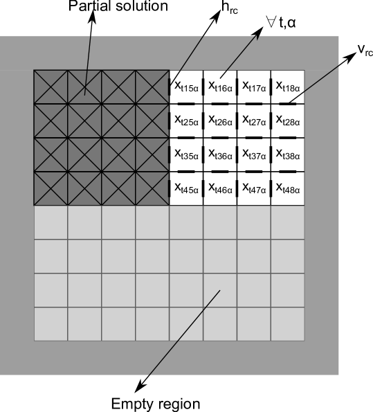
Figure 2: Illustration of how model (1)–(14) can be modified such that it only considers the positions in a region $(1,4)\times(4,8)$, given a partial solution $S^{\ast}$ on region $(1,1)\times(4,4)$.

This partial optimization model can be applied to solve all regions sequentially, thus constructing the final complete solution. Initially $R_{1}$ is optimised, after which region $R_{2}$, disjoint from region $R_{1}$, is optimised, and so on. The variables corresponding with the region are then optimally assigned by the MILP solver. Algorithm 1 presents pseudocode of this approach.

Algorithm 1 Greedy heuristic

$\mathcal{R}=\{R_{1},R_{2},R_{3},\ldots R_{K}\}$ $\triangleright$ A decomposition of $R$ in $K$ regions $R_{i}$

$T^{\ast}_{0}\leftarrow\emptyset,R^{\ast}_{0}\leftarrow\emptyset,S^{\ast}_{0}\leftarrow\emptyset$ $\triangleright$ The initial partial solution $S^{\ast}$ has no tiles assigned

for $i=1,\ldots,K$ do

    $S^{\ast}_{i},T^{\ast}_{i},R^{\ast}_{i}\leftarrow$ Apply MILP model to region $R_{i}$, given $S^{\ast}_{i-1},T^{\ast}_{i-1}$ and $R^{\ast}_{i-1}$.

    $\triangleright$ Get a new partial solution $S^{\ast}_{i}$, with tiles assigned to $R_{i}$

end for

return $S^{\ast}_{K}$

For each puzzle’s size, differently sized subsets of tiles have been tested to assess the quality of the approach. Preliminary tests of regions varying from 2 by 2 tiles (size 4) to 16 by 2 tiles (size 32) have been performed on the EII puzzle instance. This preliminary analysis revealed that the CPU time required at each iteration of the greedy heuristic limits the subset size to 32 tiles. This roughly corresponds to 32500 MILP variables for the first region of the real EII puzzle. Clearly, an increased number of tiles leads to better results. However, more CPU time is needed to compute the optimal solution, limiting the use in any hybrid framework.

3.2 MILP-based backtracking constructive heuristic

A backtracking version of the greedy heuristic has also been developed. The main idea, namely building a complete solution by constructing optimal regions, is the same as for the greedy heuristic. The backtracking version, however, restricts the optimal value of each subproblem to zero. All tiles in the region should match both internally and with respect to the tiles outside the region. Whenever a subproblem is determined to be infeasible (i.e. no completely edge matching region can be constructed), the procedure backtracks to the previous region in order to find a new assignment in that region. This may afterwards enable constructing a feasible assignment in the next region. If not, then the process is repeated until the backtracks are sufficient to find a complete solution.

Model (1)–(14), suitably modified, is again used to build partial solutions. Let $R_{i}$ be the current region considered by the procedure and $S_{i}^{\ast}$ the related partial solution once the corresponding MILP model is solved. Whenever the lower bound of the MILP model related to region $R_{i}$ is detected to be greater than zero, optimisation of region $R_{k}$ is stopped. Instead, the previous region $R_{i-1}$ is reconsidered in order to obtain a new partial solution $S_{i-1}^{\prime\ast}$, again with value $0$. Let $X_{i-1}^{*}$ be the set of variables ${x}_{t,r,c,\alpha}$ having value $1$ in solution $S_{i-1}^{*}$. The previous partial solution $S_{i-1}^{\ast}$ must be cut off when searching for solution $S_{i-1}^{\prime\ast}$. The following new constraint is added to the model:

$$\sum_{\hskip 56.9055ptt,r,c,\alpha\;:\;x_{t,r,c,\alpha}\in X_{i-1}^{*}}x_{t,r,c,\alpha}\leq|X_{i-1}^{*}|-1$$ (17)

The rationale is to force at least one of the variables of set $X_{i-1}^{*}$ to be equal to zero. If no solution of the previous region $R_{i-1}$ can lead to a zero lower bound in the current region $R_{i}$, the procedure backtracks further and searches for a new solution for region $R_{i-2}$ (and so on).

Due to the enumerative nature, this procedure can lead to incomplete solutions despite long computation times. We decided to limit the backtracking procedure to a fixed time limit, after which the greedy heuristic continues until a complete solution is generated. This backtracking heuristic is sketched in Algorithm 2, in which a recursive method ($BACKTRACKING\_HEURISTIC$) attempts to solve the current region $R_{i}$, given partial solution $S^{\ast}_{i-1}$ obtained in the previous region $R_{i-1}$. If the lower bound $lb$ of the current region is greater than 0, the method backtracks to the previous level. However, if the lower bound is still $0$ (and a perfectly matched assignment is found), the heuristic attempts to solve the next region. This will continue calling recursively until the puzzle is solved, or shown infeasible given the current assignments in $S^{\ast}_{i-1}$. In the latter case, the current partial solution $S^{\ast}_{i-1}$ will be excluded and a new partial solution $S^{\prime\ast}_{i-1}$ will be constructed, different from $S^{\ast}_{i-1}$ and any other previously excluded partial solution.

If a timeout is reached, the method will continue with the best partial solution and solve the remaining regions with the greedy heuristic, discussed in the previous section.

Algorithm 2 $BACKTRACKING\_HEURISTIC$

$\mathcal{R}=\{R_{1},R_{2},R_{3},\ldots R_{K}\}$ $\triangleright$ A decomposition of $R$ in $K$ regions $R_{i}$

$i$ $\triangleright$ Current recursive level ($i=1,\ldots,K$)

$S^{\ast}_{i-1}:T^{\ast}_{i-1}\mapsto R^{\ast}_{i-1}$ $\triangleright$ Partial solution of the previous level ($S^{\ast}_{0}$ is the initial empty partial solution)

$excludedsolutions\leftarrow\emptyset$ $\triangleright$ Partial solutions not leading to feasible solutions

while not timeout do

    $S^{\ast}_{i}\leftarrow OPTIMIZE\_REGION(S^{\ast}_{i-1},R_{i},excludedsolutions)$

    if $lb>0$ then

         return $S^{\ast}_{i-1}$ $\triangleright$ No feasible solution in current level. (backtrack)

    else

         $S^{\ast}_{i+1}\leftarrow BACKTRACKING\_HEURISTIC(\mathcal{R},i+1,S^{\ast}_{i})$

         if $S^{\ast}_{i+1}=S^{\ast}_{i}$ then $\triangleright$ $S^{\ast}_{i}$ does not lead to feasible solution

             $excludedsolutions\leftarrow excludedsolutions\cup S_{i}^{\ast}$

         else

             $S^{\ast}\leftarrow S^{\ast}_{i+1}$ $\triangleright$ $S^{\ast}_{i+1}$ is the complete solution

             return $S^{\ast}$

         end if

    end if

end while

$S^{\ast}\leftarrow GREEDY(S^{\ast}_{i},R^{\ast}_{i})$

return $S^{\ast}$

3.3 A multi-neighbourhood local search approach

A multi-neighbourhood local search approach has been developed to improve the solutions generated by the constructive heuristics (or any random solution). The key idea is to test, after an initial, complete solution is generated by the heuristics, whether a controlled-size neighbourhood can still improve the current solution. This local search method is a Steepest Descent search that tries to improve a solution with the following neighbourhoods: Border Optimisation, Region Optimisation, Tile Assignment and Tiles Swap and Rotation. We refer to Figure 3 for an illustration of the regions considered by these neighbourhoods.

The Border Optimisation (BO) neighbourhood only considers placing tiles in the border, while all the tiles in the inner part are fixed. The decomposition tries to find the optimal border in terms of matching edges, also considering the fixed tiles on the adjacent inner part. Correspondingly, model (1)–(14) is modified in such a way that the inner tile/positions variables are fixed to their current value. Only the border tile/positions variables can change value. This subproblem corresponds to a one-dimensional edge-matching problem. Preliminary computational tests indicated that the related MILP model could always be solved. Solutions for the largest instances, such as the original EII puzzle, can be generated within little computation time. When the BO neighborhood is considered, the corresponding MILP model is solved, returning a solution at least as good as the current solution and consisting of an optimal border with respect to the $(n-2)\times(n-2)$ inner region.

The Region Optimisation (RO) neighbourhood relates to the optimisation of a smaller region inside the puzzle and only considers the tiles of this region in the puzzle. Correspondingly, given the current solution, model (1)–(14) is suitably modified in such a way that the tile/position variables outside the region are fixed to their current value. Only the region’s tile/position variables can change value. The RO neighborhood can also be tackled by means of the Max-Clique formulation by generating a graph only containing nodes corresponding to tile/position assignments in the specified region. However, only feasible tile/position assignments should be considered and nodes conflicting with assignments adjacent to (but outside) the region should not be added to the graph. We recall that the purpose of the model is to find complete assignments, that is, without any unmatched edges. However, given the tiles in the considered region, it may not be feasible to find such a solution. In this case, holes are left in the region to which the remaining, unassigned tiles should be assigned. The related MILP region model is solved where all assigned tile/position variables are fixed to the value determined by the Max-Clique solver. When the RO neighborhood is considered, the local search procedure samples regions of fixed size in the current solution under consideration. For small sizes, the Max-Clique model (heuristically) is solved faster than the MILP model. Therefore, the RO neighborhood is always addressed by means of the Max-Clique formulation where the MILP formulation is only used for completing the solution whenever holes are left in the region.

In the Tile Assignment (TA) neighbourhood, $k$ tiles are removed from non-adjacent positions (diagonally adjacent is allowed) and optimally reinserted, thereby minimising the number of unmatched edges. The related subproblem corresponds to a pure bipartite weighted matching problem, which is optimally solvable by e.g. the Hungarian Algorithm [9]. The TA neighbourhood was first introduced by Schaus and Deville [11] who called it a very large neighbourhood. Wauters et al. [14] developed a probabilistic version of the TA neighbourhood that sets a higher probability to selecting tiles with many unmatched edges. The latter TA variant was applied in the present paper. The TA separates the inner and the border moves. It is prohibited to reassign border pieces to the inner region and vice versa.

An extention to the TA neighbourhood is also tested. In particular a “checkers” configuration of selected tiles is studied, i.e. all tiles on the board that are diagonally adjacent. We denote this extension Black and White (BW). The local search procedure iterates in this neighbourhood, iteratively changing between “black” and “white” positions and solving the related bipartite weighted matching problem until no more improvements are found.

Finally, the Tiles Swap and Rotation (TSR) neighbourhood is a standard local search swap operator, in this case swapping the assignment of two tiles, trying all possible rotations as well. The local search procedure exhaustively searches the neighbourhood until a local optimum is reached.

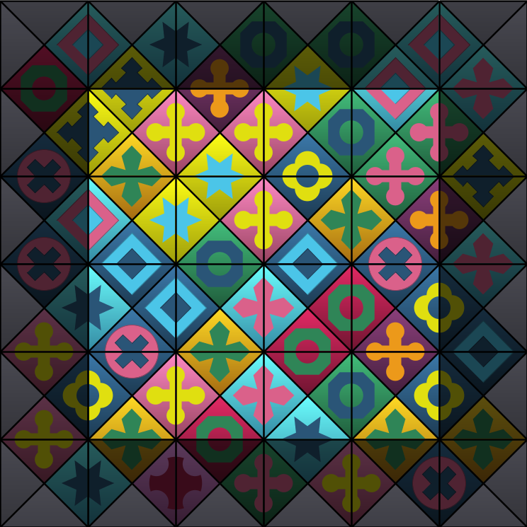
(a)

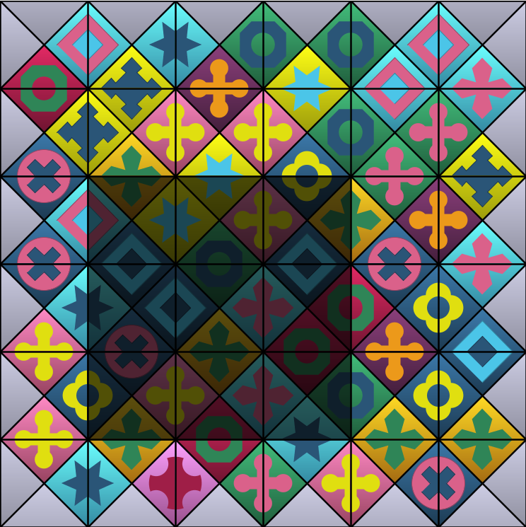
(b)

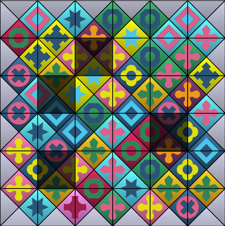
(c)

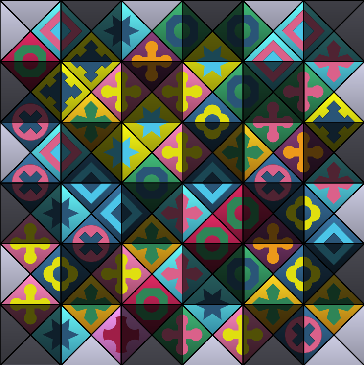
(d)

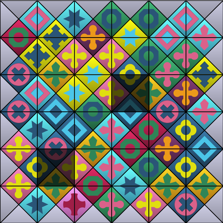
(e)

Figure 3: Illustration of the regions involved in the neighbourhood operations: LABEL:sub@subfig:bo optimizing the border (BO); LABEL:sub@subfig:ro optimizing a rectangular region (RO); LABEL:sub@subfig:ta optimizing non-adjacent tile assignments (TA); LABEL:sub@subfig:bw optimizing diagonally adjacent tile assignments in a checkers fashion (BW); LABEL:sub@subfig:tsr swapping two tiles and possibly rotating them (TSR).

4 Computational Results

This section provides computational results obtained by the multi-neighbourhood local search approach on the Eternity II puzzle as well as the $10\times 10$, $12\times 12$, $14\times 14$ and $16\times 16$ instances that were used in the META 2010 EII contest. The latter instances serve as an interesting test set for comparison, due to the availability of some results from the contest. In addition, to the best of our knowledge, the complete solutions of these instances are not publicly available. The $3\times 3$ to $9\times 9$ instances used in Section 2 also originate from this set.

All tests were performed on a 40 cores Intel Nehalem cluster with 120 GB ram, with each core running @ 3.46 GHz with 8 MB cache. Computational resources provided by DAUIN’s HPC Initiative. This cluster was used to solve different instances/runs in parallel in order to reduce the total time required to run all tests. Each individual test was run on a single processing core, thus no parallelism was employed in the algorithms. All MILP models are solved using CPLEX 12.4.

Parameter Name	Value
$TA.K$	16 tiles
$TA.N$	1000 it
$Clique.W$	6 cols
$Clique.H$	6 rows
$Clique.N$	10 it

Table 2: Parameter Settings

Table 2 summarizes the parameter settings of the multi-neighbourhood local search approach. The local search procedure starts either from a random solution or from a solution obtained by the constructive heuristics. The algorithm cycles through the proposed neighbourhoods in the following sequence: TA (for $TA.N$ iterations with sample size $TA.K$), BO (for one iteration), BW (till local optimum), TSR (till local optimum) and finally RO by means of the Max-Clique formulation (for $Clique.N$ iterations with rectangular sample size $Clique.W\times Clique.H$). This sequence was determined experimentally, though the difference in performance between sequences was very limited. At the end of the multi-neighbourhood step, the final solution is a local minimum with respect to all considered neighbourhoods.

Table 4 shows the results for twenty runs of the MILP-based greedy heuristic and the MILP-based backtracking heuristic for different region sizes on all the problem instances. A timeout of $1200$ seconds was set for the backtracking heuristic for the $10\times 10$ instance, $1800$ seconds for the $12\times 12$ instance, $2400$ seconds for the $14\times 14$ instance and $3600$ seconds for the $16\times 16$ and EII instances. The greedy heuristic (executed by itself, or after the backtracking heuristic) is executed until all regions are solved. The table also shows the results of both constructive methods after subsequent optimisation by the local search heuristic.
In general, both constructive heuristics generate better results when larger regions are used. This clearly affects the CPU time needed to compute optimal solutions for each region. By comparing the results of the two heuristics (without the local search phase), it seems that the backtracking procedure does not strongly dominate (on maximum, average and minimum values) the greedy one, while consuming all the available time. This dominance tends to be more evident for small puzzles and region sizes, while for larger instances with solutions generated by larger regions, the gap becomes smaller.

In almost all cases, the local search procedure manages to improve the results of the constructive heuristics by several units, indicating that these initial solutions are not local optima with respect to the considered neighbourhoods. We conclude that many neighbourhoods in a complex structure are effective for improving these greedy constructive solutions. Table 4 shows the performance of the local search procedure starting from a random initial solution of poor quality. The procedure can achieve good quality results for the $10\times 10$ instance, but not for larger instances. This can easily be related to the size of the RO neighborhood. As it is quite large with respect to the puzzle size in the $10\times 10$ instance, it is able to optimize a large part of the puzzle. However, this ratio becomes smaller and is thus less effective for larger instances.

Finally, Table 5 compares the best published results with the results obtained by the hybrid local search procedure. The CPU times refer to the considered time limits. Table 5 also reports a large test of the procedure, where the best performing configuration (backtracking+LS) was run 100 times within a doubled execution time limit. Larger execution times (using CPLEX 12.4 as ILP solver) do not induce further improvements of the results. We note that some of the entries of Table 5 are missing. Many of the approaches only deal with a subset of the considered instances. Only three studies [4, 13, 14] report results for the $10\times 10$ to $16\times 16$ instances that were tested in this paper. Some approaches [11, 10, 12] were only applied to the real EII game puzzle.

The algorithm reported in [11] was executed on a CPU Intel Xeon(TM) 2.80GHz, with computation time 24 hours. The best score over 20 runs equals 458.
[10] obtained a best score of 371. No indication was provided on the computer and the required CPU time.
The algorithm of [4] was run on a PC Pentium Core 2 Quad (Q6600), 2.4 GHz, with 8 GB of RAM. It considered EII style problems (but not the real puzzle) with sizes $10\times 10$, $12\times 12$, $14\times 14$ and $16\times 16$. The corresponding time limits were 1200, 1800, 2400 and 3600 seconds respectively and the entries of Table 5 report the best solution obtained over 30 runs.
The algorithm of [13] addressed the same instances with the same time limits and number of runs as [4]. It was tested on a personal computer with 1.8GHz CPU and 1GB RAM. Time limits and number of runs were the same as in [13]. The tests were performed on an Intel Core 2 Duo @ 3Ghz with 4GB of RAM.
The algorithm of [14] was tested on all the instances from [4] and [13] and also on the EII real game puzzle. The entry reports the best result obtained over 30 runs with a time limit of 3600 seconds for EII.
Finally, the algorithm of [12] was tested on the EII real game puzzle only running on a grid computing system over a period of several weeks/months not explicitly indicated by the authors.

The results show that the algorithm is competitive with the state of the art, obtaining top results for the $10\times 10$ instance in a similar time frame as the other algorithms. Most interesting, the initial solution constructed by the greedy and backtracking heuristics is already of high quality, leaving only a limited gap from the optimal solution. Therefore, we expect that these methods may serve as the basis for reaching new top results. The best result for the official EII puzzle instance, 467 obtained using a slipping tile, scan-row backtracking algorithm [12], is still out of our current grasp. However, that algorithm was highly tailored to the EII puzzle instances, used precomputed sequences and was run over the course of several weeks/months (see http:$//$www.shortestpath.se$/$eii$/$eii$\_$details.html). A direct comparison with the approach presented is partially misleading. Among the other existing approaches, only [14] shows to be slightly superior to our approach. However, our approach should become more competitive along with the expected performance improvement of MILP solvers over the years. Clearly, solving larger subregions in both the constructive heuristics (greedy and backtracking) will lead to better initial solutions. In addition, the effectiveness of the MIP-based local search neighbourhoods is expected to improve when larger regions can be solved. If performance improvements allow ILP solvers to address instances of size $8\times 8$ or even $9\times 9$ in a reasonable amount of time, it may safely be assumed that the proposed approach will lead to improved results competitive with the other state of the art approaches.

INSTANCE	START	Region Size	MAX	AVG	MIN	Time Avg. (s)
10x10	greedy	1 x 10	165	161.10	158	4.29
	greedy+LS	1 x 10	168	164.90	161	1204.29
	greedy	2 x 10	170	166.35	164	25.93
	greedy+LS	2 x 10	170	167.05	164	1225.93
	backtracking	1 x 10	169	165.65	162	1200.24
	backtracking+LS	1 x 10	172	167.75	165	2400.24
	backtracking	2 x 10	170	167.65	164	1207.06
	backtracking+LS	2 x 10	171	168.10	165	2407.06
12x12	greedy	1 x 12	245	241.20	239	6.83
	greedy+LS	1 x 12	247	244.00	240	1806.83
	greedy	2 x 12	249	247.00	244	101.02
	greedy+LS	2 x 12	250	247.50	245	1901.02
	backtracking	1 x 12	248	245.35	242	1801.51
	backtracking+LS	1 x 12	250	247.75	246	3601.51
	backtracking	2 x 12	249	247.60	246	1868.85
	backtracking+LS	2 x 12	252	248.45	246	3668.85
14x14	greedy	1 x 14	338	333.00	329	10.43
	greedy+LS	1 x 14	339	335.56	332	2410.43
	greedy	2 x 14	344	340.50	338	2335.42
	greedy+LS	2 x 14	344	340.80	338	4735.42
	backtracking	1 x 14	342	338.25	334	2401.36
	backtracking+LS	1 x 14	344	340.69	336	4801.36
	backtracking	2 x 14	344	342.17	340	4664.65
	backtracking+LS	2 x 14	344	342.33	340	7064.65
16x16	greedy	1 x 16	448	444.05	440	24.08
	greedy+LS	1 x 16	449	446.20	443	3624.08
	greedy	2 x 16	454	451.38	448	11188.03
	greedy+LS	2 x 16	454	451.88	448	14788.03
	backtracking	1 x 16	453	448.80	444	3605.68
	backtracking+LS	1 x 16	454	451.53	449	7205.68
	backtracking	2 x 16	457	453.69	451	13722.86
	backtracking+LS	2 x 16	457	454.00	451	17322.86
EII-instance	greedy	1 x 16	449	443.75	440	21.85
	greedy+LS	1 x 16	450	446.50	442	3621.85
	greedy	2 x 16	456	451.75	450	13835.04
	greedy+LS	2 x 16	457	451.95	450	17435.04
	backtracking	1 x 16	453	449.00	446	3605.08
	backtracking+LS	1 x 16	454	451.35	447	7205.08
	backtracking	2 x 16	457	452.80	448	15294.52
	backtracking+LS	2 x 16	457	453.15	449	18894.52

Table 3: Results for the MILP-based greedy and backtracking heuristics with and without local search, using different region sizes.

	$\mathbf{10\times 10}$	$\mathbf{12\times 12}$	$\mathbf{14\times 14}$	$\mathbf{16\times 16}$	$\mathbf{EII-instance}$
$\mathbf{Obj_{Max}}$	167	238	312	398	391
$\mathbf{Obj_{Avg}}$	163.2	231.1	299.2	384.3	382
$\mathbf{Obj_{Min}}$	158	223	292	367	372
Optimum	180	264	364	480	480

Table 4: Results for the local search procedure with optimal neighbourhoods starting from a random solution.

	$\mathbf{10\times 10}$	$\mathbf{12\times 12}$	$\mathbf{14\times 14}$	$\mathbf{16\times 16}$	$\mathbf{EII-instance}$
Present paper (20 runs)	172 (20 min)	252 (30 min)	344 (40 min)	457 (180 min)	457 (180 min)
Present paper (100 runs)	172 (40 min)	252 (60 min)	347 (80 min)	457 (360 min)	458 (360 min)
Muñoz et al. [10]	-	-	-	-	371 (-)
Wang and Chiang [13]	163 (20 min)	234 (30 min)	318 (40 min)	418 (60 min)	-
Coelho et al. [4]	167 (20 min)	241 (30 min)	325 (40 min)	425 (60 min)	-
Schaus and Deville [11]	-	-	-	-	458 (1440 min)
Wauters et al. [14]	172 (20 min)	254 (30 min)	348 (40 min)	460 (60 min)	461 (60 min)
Verhaard [12]	-	-	-	-	467 (weeks/months)
Optimum	180	264	364	480	480

Table 5: Comparison of the best results to other approaches available in the literature. (Execution times presented within parenthesis)

5 Conclusions

The present work introduced a hybrid approach to the Eternity II puzzle. A MILP formulation is related to the puzzle’s optimisation version, where the total number of unmatched edges should be minimised. It is shown that the Eternity II puzzle can be modelled as a clique problem, providing, as a byproduct of this work, new hard instances of the maximum clique problem to the community. Preliminary testing revealed it was clear that these models cannot handle large size instances (such as the original EII puzzle), as they quickly become computationally intractable. Therefore, these models were used as the basis for heuristic decompositions, which could then be used in a hybrid approach.

A greedy and a backtracking constructive heuristic have been designed, which strongly rely on the capability of optimally solving a specific region of the puzzle. Within a reasonable time limit, high quality solutions can be generated using these heuristics. A multi-neighbourhood local search approach has also been proposed. By applying a set of different neighbourhoods, the local search procedure manages to improve upon the initial solutions generated by the constructive heuristics and reaches solutions competitive to the best available results.

These results confirm that a novel and clever use of mathematical models and solvers/heuristics is effective for large size problems, which cannot be solved all in once by the same MILP solver. We believe that hybridizing local search approaches and mathematical programming techniques in a matheuristic context is the key to break up the intractability of hard problems such as the EII puzzle.

References

- [1] Ansótegui C, Béjar R, Fernàndez C, Mateu C. Edge matching puzzles as hard SAT/CSP benchmarks. In: CP ’08 Proceedings of the 14th international conference on Principles and Practice of Constraint Programming, 560-565, 2008.
- [2] Benoist T, Bourreau E. Fast global filtering for Eternity II. Constraint Programming Letters, 3, 35-50, 2008.
- [3] Bomze IM, Budinich M, Pardalos PM, PelilloM. The maximum clique problem. In: Du DZ, Pardalos PM (eds) Handbook of combinatorial optimization. Kluwer Academic, Dordrecht, 1–74, 1999.
- [4] Coelho I, Coelho B, Coelho V, Haddad M, Souza M, Ochi L. A general variable neighborhood search approach for the resolution of the Eternity II puzzle. In: Proceedings of the 3rd International Conference on Metaheuristics and Nature Inspired Computing, META’10. 2010, http://www2.lifl.fr/META10/proceedings//meta20100submission157.pdf.
- [5] Demaine ED, Demaine ML. Jigsaw puzzles, edge matching, and polyomino packing: Connections and complexity. Graphs and Combinatorics, 23, 195-208, 2007.
- [6] Grosso A, Locatelli M, Pullan W. Simple ingredients leading to very efficient heuristics for the maximum clique problem. Journal of Heuristics, 14, 587-612, 2008.
- [7] Heule MJH. Solving edge-matching problems with satisfiability solvers. In: Proceedings of the Second International Workshop on Logic and Search (LaSh 2008), 88-102, 2008.
- [8] Kendall G, Parkes A, Spoerer K. A survey of NP-Complete puzzles. International Computer Games Association Journal, 31, 13-34, 2008.
- [9] Kuhn HW. The Hungarian Method for the assignment problem. Naval Research Logistics Quarterly, 2, 83-97, 1955.
- [10] Muñoz J, Gutierrez G, Sanchis A. Evolutionary genetic algorithms in a constraint satisfaction problem: Puzzle Eternity II. In: Cabestany J, Sandoval F, Prieto A, Corchado J, editors. Bio-Inspired Systems: Computational and Ambient Intelligence; LNCS 5517, 720-727, 2009.
- [11] Schaus P, Deville Y. Hybridization of CP and VLNS for Eternity II. In: JFPC’08 Quatrième Journées Francophones de Programmation par Contraintes. 2008, http://www.info.ucl.ac.be/yde/Papers/JFPC2008Eternityen.pdf.
- [12] Verhaard L. http://www.shortestpath.se/eii/index.html; 2008.
- [13] Wang WS, Chiang TC. Solving eternity-ii puzzles with a tabu search algorithm. In: Proceedings of the 3rd International Conference on Metaheuristics and Nature Inspired Computing. 2010, http://www2.lifl.fr/META10/proceedings//meta20100submission161.pdf.
- [14] Wauters T, Vancroonenburg W, Vanden Berghe G. A guide-and-observe hyper-heuristic approach to the Eternity II puzzle. Journal of Mathematical Modelling and Algorithms, 11, 217-233, 2012.