Reheating constraints through decaying inflaton
Abstract
In this paper we study the reheating constraints on inflationary models considering perturbatively decaying inflaton. Important difference with the existing analysis is the inclusion of explicit decaying dynamics of inflaton during reheating. One of the important findings of our analysis is the possible existence of maximum reheating temperature considering perturbative reheating scenario. For all the models under consideration the value of this temperature turned out to be GeV. Corresponding to this value of reheating temperature the duration of reheating period assumes naturally small value, which indicates instantaneous reheating. Most importantly, maximum reheating temperature also leads to a maximum values of scalar spectral index and inflationary e-folding number in association with the observed CMB scale. Based on our general analysis, we have studied four different inflationary models, and discuss their predictions and constraints.
After the inflation, reheating is the most important phase which sets the initial condition for the subsequent standard big-bang evolution of our universe. During this phase all the visible and invisible matter fields are assumed to be produced through the decay of coherently oscillating inflaton field. Therefore, not only inflaton encyclopedia but details of its inflationary dynamics is expected to have strong influence on the dynamics of reheating. Cosmic Microwave Background (CMB) is crucially dependent upon the background expansion starting from the radiation phase to the present epoch. Therefore the observed CMB scales and their horizon exit during inflation must be correlated through reheating phase. Reheatingreheating is the integral part of the inflationary paradigm. However, complicated thermalization process erases many details of this phase. Understanding this phase could answer many unanswered questions such as inflationary mechanism itself, baryogenesis, origin of dark matter etc. A model independent approach has recently been adopted martin to analyze this phase. In this approach the main idea was to parametrize the phase by an effective equation of state , and there by constrain it by e-folding number and the reheating temperature through the inflationary parameters. A large class of inflationary models have been studied based on this idea martin ; reheatingfollows . Recently there are attempts to consider the explicit decay of inflaton into the analysis decay , and subsequently its application to specific inflationary models decayfollows . Constraining the reheating temperature through decaying inflation has also be considered reheatingtemp . However, all the analysis so far were done based on identifying effective fluid with the reheating equation of state , and finally express the perturbative reheating temperature in terms of inflaton decay constant. Therefore, the process of decaying inflaton during reheating has not been considered explicitly in the analysis.
As has been mentioned before, our goal in the present paper will be to study the reheating constraints considering the effect of perturbative decay of inflaton into the dynamics of radiation and inflaton. Therefore, important parameter of our analysis is the inflaton decay constant. We further assume that the inflaton decays only into the relativistic fields collectively called as radiation.
General analysis: After inflation, the inflaton oscillates around its minimum and reheating phase starts. Depending upon the coupling parameters, non-perturbative reheating may occur. However, as emphasized before, we ignore non-perturbative reheating for the present purpose.
We start with the following Einstein’s equation for the cosmological scale factor and conservation of energy,
| (1) | |||
Where, ””s are the energy densities of two different components. At any instant of time during reheating, we parametrize the duration of reheating by e-folding number , where ”” is the cosmological scale factor. During reheating if we assume the effective equation of state of the inflaton to approximately constant, the above conservation equation turned out to be
| (2) |
The index ”i” stands for the initial stage of reheating, which also marks the end of inflation. At the beginning of reheating we set . For solving the above set of equations, the boundary condition is . The physical quantity of our interest is the ratio of the radiation energy density and the inflaton energy density. From eq.2, one gets
| (3) |
Where, ”f” corresponds to the final value of radiation density. We define total e-folding number during reheating as .
The main goal is to understand the relation among inflaton’s energy density , the radiation temperature and the CMB scale . A particular scale going out of the horizon during inflation will re-enter the horizon during usual cosmological evolution. This fact will provide us an important relation among different phases as follows
| (4) |
where, a particular scale satisfy the relation . , are the cosmological scale factors at the end of reheating phase and at the present time respectively. are the efolding number and the Hubble parameter respectively during inflation. is the present value of the Hubble constant.
The usual approach so far was to define the effective equation of state of the total energy density during reheating and study its evolution. However, we consider only the radiation part during reheating and try to understand the evolution of its temperature as a function of scalar spectral index associated with CMB scale. The reheating temperature is identified with radiation temperature at thermal equilibrium between the decaying inflaton and the radiation. From the entropy conservation of thermal radiation, the relation among , and , temperature of the CMB photon and neutrino background at the present day respectively, can be written as
| (5) |
Using eq.(4,5), one arrives at the following well known relation
| (6) |
Where, is the effective number of relativistic degrees of freedom during radiation phase. In our subsequent study we identify the cosmological scale as the pivot scale set by PLANCK, and compare our result with the corresponding estimated scalar spectral index PLANCK .
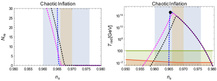
Exactly solvable case: In order to understand the possible existence of maximum reheating temperature, we first consider an analytically solvable model where the inflaton is decaying as
| (7) |
is a dimensionless constant,
which parametrizes the decay of inflaton. This form of decay essentially modifies the Hubble friction term for the dynamics of inflaton during reheating. With aforementioned ansatz for the decaying inflaton, the solution for radiation density turned out to be
| (8) |
The second term in the parenthesis is quantifying the fractional amount of inflaton energy left after the reheating process is over. Expressing in term of radiation temperature as , the eq.8 leads to a maximum radiation temperature for a given as
| (9) |
where, . This also can be clearly seen from the Fig.1 for each value of . Now from the perturbative point of view, the value of . However, if we naively extrapolate the above result for large most important result turned out to be the existence of a maximum possible temperature,
| (10) |
And this value is numerically of the order of same as for limiting perturbative value at as shown in the figure Fig.1. Therefore, above temperature can be naturally identified as maximum possible reheating temperature. Considering eq.6, this also corresponds to a maximum possible value of scalar spectra index at that temperature. Now identifying associated temperature of the produced radiation in eq.8 with eq.6, we arrive at the following exact expression for ,
| (11) | |||
| (12) |
In the fig.1, we have considered three possible values of for quadratic inflaton potential. The special value is , for which the equilibrium condition between the inflaton and the radiation can be achieved at the maximum temperature shown as a black dot. The maximum value of scalar spectral index turned out to be . This analysis motivates us to subsequently analyze more general cases, and we will show that this conclusion still holds.
General case: In this section we will consider general perturbatively decaying inflaton. For this case, we express the decaying inflaton as
| (13) |
Where is effective time independent inflaton decay constant. However, we believe our conclusion will remain same for time dependent , which we will study later. Before numerical analysis, let us examine the approximate solution which has already been discussed in the literature tmax . During the early stage of evolution, approximating , the radiation density can be calculated as
| (14) |
As has been discussed for the exactly solvable case in eq.9, above equation also leads to a maximum radiation temperature tmax for a given ,
| (15) |
Where, the relation has been used. In the same way as we have discussed in the previously discussed exactly solvable case, maximum possible temperature could be obtained, if one identifies a special point where two temperature meets, . Our numerical analysis also shows the maximum reheating temperature at the aforementioned special point,
| (16) |
The maximum reheating temperature can also be computed for another exactly solvable case with . The corresponding result is as follows,
| (17) | |||||
This expression is exactly the same as previously discussed case. For this special value of , we also have exact expression for parameters as
| (18) | |||
| (19) |
At this point let us again emphasize the fact that as long as we are in the perturbative regime, the relation among the scalar spectral index and the reheating temperature can be understood from our detail analysis above. However, existence of maximum reheating temperature will come if we extrapolate all our formulas for large . For low scale inflation, could always be in the perturbative regime. However, for large scale inflation, which we will be considering the system could be in the non-perturbative regime. The detail analysis we will take up for our future publication. To this end, we would like to point out that in the effective reheating equation of state description martin , the maximum temperature can be explained in the limit of zero reheating e-folding number . Therefore, large limit in our analysis can be thought of as an equivalent to the zero limit of the previously studied reheating constraint studies.
The main point of our is to understand the dynamics of decaying inflaton in the reheating constraint analysis. We think this is the appropriate procedure to understand the relation among . In the subsequent discussions, we consider different models their predictions.
Numerical study and constraints: For general case let us first describe the strategy of our numerical study. We identify the inflation model dependent input parameters as for a particular CMB scale . Given a canonical inflaton potential , the inflationary efolding number and Hubble constant can be expressed as
| (20) |
were, the field values are computed form the condition of end of inflation,
| (21) |
and equating a particular value of scalar spectral index with . Therefore, we will get explicit relations between and . The reheating parameters will implicitly depend on the scalar spectral index for a given scale.
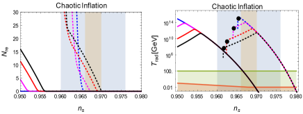
Associated with each value of , if we assume the radiation domination starts at , present CMB scale eq.(6), fixes the corresponding value of the scalar spectral index. In plot we have three distinct regions. In the high region, the reheating time parametrized by is significantly small. Therefore, increases with the increasing through the specific function till the maximum is reached. In this region, the amount of radiation transfered is significantly small unless we are at the maximum reheating temperature where instant reheating happens. In the intermediate region, increasing starts playing role and decreases towards reheating temperature where decaying inflaton and radiation equilibrates. We have taken four sample values of decay constants and corresponding respectively. The aforementioned equilibrium condition fixes the reheating temperature of our universe as Therefore, corresponding perturbative reheating temperatures are GeV. We marked those points as black dots in fig.2. In addition for a given inflaton-radiation equilibrium state during reheating in association with the present CMB scale corresponds to a specific value of inflationary scalar spectral. At the equilibrium temperature perturbative decay of inflaton is expected to be maximum and reheating is assumed to be completed. As expected after this the radiation density falls very fast, therefore, temperature of the radiation will also fall very fast as we decrease .
However, the most interesting point of our analysis is the existence of maximum temperature in eq.15. This is clearly seen from all the plots for different models under consideration. At this temperature, the intermediate region shrinks to zero at . The interplay between the observed CMB scale and the dynamics of inflation limit the aforementioned for all the models we have considered. It is also interesting that associated with this , eq.6 and eq.15 predicts maximum value of scalar spectral index and inflationary e-folding number associated with the CMB scale. Therefore, is the maximum possible reheating e-folding number required to explain the observed CMB scale assuming the perturbative reheating. In the following discussions we consider various models, and study their predictions and constraints.
Chaotic chaotic inflation
As has been emphasized, for the canonical inflationary models, potential will contain all the information. For usual chaotic inflation the potential looks like,
| (22) |
Where . If we consider only the absolute value of the field, can also be included. The average equation of state of the inflaton during reheating is taken as . As has been mentioned before, the black dots in Fig.2, correspond to reheating temperature for different value of .
For case, within the blue shaded () region of , the combined effect of CMB measurement and the inflation provide the following limit , and in GeV unit. Therefore, for chaotic inflation, the maximum value of scalar spectral index . It is also clear from the figure that for or in other word if the inflaton field behaves like a radiation during reheating, prediction of is well outside the observed CMB limit as seen in Fig.2. Therefore, all models with are strongly disfavored considering the perturbative reheating scenario.
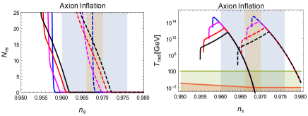
Axionaxion inflation
The potential for the axion/natural inflation is
| (23) |
where, are the scale of inflation and axion decay constant respectively. The CMB normalization fixes the over all scale of inflation . Therefore, by tuning the model can be made compatible with observation as seen in Fig.3. Because of quadratic form of the axion potential near the minimum, we chose in our analysis. The over all behavior of the in terms of is similar as for the chaotic models. We have chosen two sample values of axion decay constant . is disfavored as it predicts maximum value of which is outside the region. However for , we have , and in GeV unit. Interestingly, turned out to be equal to the central value of observed in CMB. Therefore, larger value of axion decay constant is favored for the axion model.
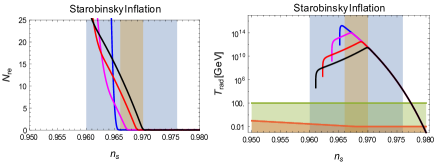
Starobinskistarobinsky /Higgshiggs inflation
Both of the inflation models are fundamentally different in their non-canonical form. However, after the canonical normalization, both the models transform into usual scalar tensor model with the same form of potential as follows,
| (24) |
where the dimension full parameter takes the following forms,
| (25) |
Prefixes, stand for Starobinsky and Higgs model respectively. The aforementioned coupling parameters appear in the non-canonical Lagrangian are as follows,
| (26) | |||
where, is the Ricci scalar in the Jordan frame. For the Higgs inflation model one assumes during inflation. The inflaton degree of freedom in the eq.24, are expressed as,
in unit of . For these system we again consider the equation of state . In both these models once we fix the CMB normalization, there is no free parameter to control. Therefore, predictions for both the models are same and quantitatively similar to the chaotic inflation. From the Fig.4, we clearly see the combined effect of CMB measurement and the inflation puts following limit , and in GeV unit. In the table 1, we summarize all our important predictions for the models we have studied.
| Chaotic | Axion | Starobinsky/Higgs | |
|---|---|---|---|
| 0.96560 | 0.9682 | 0.96548 | |
| 57.6 | 57.2 | 55.8 | |
| 0.30 | 0.32 | 0.34 |
Summary and discussion: One of the main assumptions of our analysis is perturbative decay of inflaton. We have considered two different types of perturbative decay processes. Irrespective of the different decay processes, the important out come of our analysis is the existence of maximum reheating temperature GeV which is nearly independent of the models we have studied. This universality is because of slow roll condition which sets the almost same boundary condition for all the models under consideration. In association with the maximum temperature, the relation between the observed CMB scale and its horizon exit during inflation yields a maximum possible scalar spectral index and e-folding number during inflation, which we have shown in the table 1. Therefore, considering the explicit decay process into the analysis, the reheating has further restricted the model parameters and even exclude some models. For example without considering the tensor spectral index, our analysis excludes power law potential form with .
It would be interesting to further generalize our analysis to consider other decay channels. Generalizing our analysis for more general class of inflationary models such as recently found -attractor alpha could be interesting. One of the assumptions of our analysis is time independent and . Depending upon particular model of reheating, can depend on the background time dependent inflaton field. Therefore, most important generalization of our analysis would be to consider time variation of . We will take up all these questions for our future publications.
References
- (1) A. H. Guth, Phys.Rev. D 23, 347356 (1981); A. D. Linde, Phys. Lett. B 108, 389393 (1982); A. Albrecht and P. J. Steinhardt, Phys. Rev. Lett. 48, 12201223 (1982); J. Martin, C. Ringeval and V Vennin, Phys. Dark Univ. 5-6 (2014) 75-235.
- (2) L. Kofman, A. D. Linde and A. A. Starobinsky, Phys. Rev. Lett. 73, 3195 (1994); L. Kofman, A. D. Linde and A. A. Starobinsky, Phys. Rev. D 56, 3258 (1997); ; Y. Shtanov, J. H. Traschen and R. H. Brandenberger, Phys. Rev. D 51 (1995) 5438.
- (3) J. Martin and C. Ringeval, Phys. Rev. D82, 023511 (2010); J. Martin, C. Ringeval and V. Vennin, Phys. Rev.Lett. 114, 081302 (2015); L. Dai, M. Kamionkowski and J. Wang, Phys. Rev. Lett. 113, 041302 (2014).
- (4) P. Adshead, R. Easther, J. Pritchard and A. Loeb, JCAP 1102, 021 (2011); R. Easther and H. V. Peiris, Phys. Rev. D85, 103533 (2012); J. B. Munoz and M. Kamionkowski, Phys. Rev. D91, 043521 (2015); J. L. Cook, E. Dimastrogiovanni, D. A. Easson and L. M. Krauss, JCAP 1504, 047 (2015).
- (5) M. Drewes, JCAP 1603, 013 (2016).
- (6) M. Drewes, J. U Kang, and U. R. Mun, arXiv:1708.01197; J. Ellis etal, JCAP 1507, 050 (2015).
- (7) M.Yu.Khlopov, A.D.Linde, Phys. Lett. 138B, 265, (1984); V. Domcke and J. Heisig, Phys. Rev. D92, 103515 (2015)
- (8) Planck Collaboration: P. A. R. Ade et al., 594, A20 (2016); Keck Array, BICEP2 Collaborations: P. A. R. Ade et al., Phys. Rev. Lett. 116, 031302 (2016).
- (9) Euclid Theory Working Group Collaboration, L. Amendola et al., Living. Rev.Rel. 16, 6 (2013).
- (10) PRISM Collaboration, P. Andre et al., [arXiv:1306.2259].
- (11) G. F. Giudice, E. W. Kolb, and A. Riotto, Phys. Rev. D64, 023508 (2001).
- (12) A. D. Linde, Phys. Lett. 129B, 177 (1983).
- (13) K. Freese, J. A. Frieman and A. V. Olinto, Phys. Rev. Lett. 65, 3233 (1990).
- (14) A. A. Starobinsky, Phys. Lett. B 91, 99 (1980).
- (15) F. L. Bezrukov and M. Shaposhnikov, Phys.Lett. B 659, 703 (2008).
- (16) R. Kallosh and A. Linde, JCAP 1307, 002 (2013); R. Kallosh, A. Linde and D. Roest, JHEP 1311, 198 (2013).