A domain-decomposition method to implement electrostatic free boundary conditions in the radial direction for electric discharges

Abstract

At high pressure electric discharges typically grow as thin, elongated filaments. In a numerical simulation this large aspect ratio should ideally translate into a narrow, cylindrical computational domain that envelops the discharge as closely as possible. However, the development of the discharge is driven by electrostatic interactions and, if the computational domain is not wide enough, the boundary conditions imposed to the electrostatic potential on the external boundary have a strong effect on the discharge. Most numerical codes circumvent this problem by either using a wide computational domain or by calculating the boundary conditions by integrating the Green’s function of an infinite domain. Here we describe an accurate and efficient method to impose free boundary conditions in the radial direction for an elongated electric discharge. To facilitate the use of our method we provide a sample implementation. Finally, we apply the method to solve Poisson’s equation in cylindrical coordinates with free boundary conditions in both radial and longitudinal directions. This case is of particular interest for the initial stages of discharges in long gaps or natural discharges in the atmosphere, where it is not practical to extend the simulation volume to be bounded by two electrodes.

PROGRAM SUMMARY

Program Title: poisson_sparse_fft.py
Licensing provisions: CC By 4.0
Programming language: Python

Nature of problem: Electric discharges are typically elongated and their optimal computational domain has a large aspect ratio. However, the electrostatic interactions within the discharge volume may be affected by the boundary conditions imposed to the Poisson equation. Computing these boundary conditions using a direct integration of Green’s function involves either heavy computations or a loss of accuracy.
Solution method: We use a Domain Decomposition Method to efficiently impose free boundary conditions to the Poisson equation. This code provides a stand-alone example implementation.

©2018. This manuscript version is made available under the CC-BY-NC-ND 4.0 license http://creativecommons.org/licenses/by-nc-nd/4.0/

1 Introduction

Despite their prevalence in industry and in nature, electric discharges still hold many unknowns. For example, we do not yet understand precisely how a lightning channel starts, how it advances in its way to the ground or how exactly are bursts of X-rays produced as it progresses [1]. This is partly due to the short time and length scales involved in such processes which, combined with their jittery behaviour, prevents the use of many diagnostic techniques. Due to these limitations, much of what we know about electric discharges comes from computer models which, at least within a simulation, are predictable and reveal arbitrarily small scales.

Consider streamer simulations. Streamers are thin filaments of ionized air that precede most electric discharges in long gaps at atmospheric pressure. The main challenge for simulating streamers is the wide separation between length scales: whereas the total length of the streamer channel at atmospheric pressure ranges from about one to some tens of centimeters, the ionization of air molecules is mostly confined to a layer thinner than one millimeter. Despite this difficulty, there are many numerical codes that explain most of the observed properties of streamers [2, 3, 4, 5, 6, 7]. In the past decades these models have gradually improved and successfully overcome many of the challenges posed by streamer physics. However, they are still computationally intensive and often require days of runtime to produce meaningful simulations.

In this work we look at one of the problems behind these long running times: the large aspect ratio of a single-channel discharge. Whereas the width of an atmospheric-pressure streamer is at most about one centimeter, its length spans many times this extension. In order to minimize the amount of work performed in a simulation, one strives to adapt the computational domain to the dimensions of the streamer, which means using a narrow cylindrical domain with a diameter only slightly larger than the streamer width. However, in such a narrow domain the electrostatic interaction between separate points in the channel is strongly affected by the boundary conditions imposed on the electric potential at the outer boundaries.

One approach to avoid this artifact while keeping a narrow domain around the streamer is to calculate the boundary values of the potential by direct integration of the electrostatic Green’s function in free space [8, 9, 10, 3, 11]. These values are then imposed as inhomogeneous Dirichlet boundary conditions in the solution of the Poisson equation. In a cartesian grid with $M$ cells in the radial direction and $N$ cells in the axial direction the direct integration of the Green’s function at each of the $N$ nodes in the external boundary requires about $MN^{2}$ operations. Since the work employed by fast Poisson solvers scales as $MN\log(MN)$ ($MN$ for multigrid solvers), the computation of boundary values by direct integration may easily dominate the work employed in the electrostatic calculations. This is mitigated in part by using a coarse-grained charge distribution in the integration. However, in that case there is a tradeoff between the degree of coarsening and the minimal radial extension of the domain required for a tolerable error.

Beyond this common approach used to solve Poisson’s equation in electric discharges, some other methods have been developed. A family of these methods has been built upon the idea of the decoupling of local and far-field effects [12] and the computation of the boundary potential by means of a potential generated by a set of screening charges located in the outer surface of the computational domain [13]. Based on these two methods mentioned above, reference [14] uses a domain decomposition approach to exploit parallel computing capabilities; first, Poisson’s equation subject to unbounded boundary conditions is solved in a set of disjoint patches. As a second step a coarse-grid representation of the space charge is obtained and Poisson’s equation is again solved in a global coarse-grid whose solution is used to communicate far-field effects to local patches. Finally, Poisson’s equation is solved in a fine grid using boundary conditions computed from the coarse-grid solution corrected with local field information.

A different family of methods uses the convolution with Green’s function subject to free boundary conditions. They manage the singular behaviour of Green’s function by either regularizing it [15], or by replacing the singular component to the integrand of the convolution by an analytical contribution [16]. These methods have achieved an order of convergence greater than two.

Here we adapt to the cylindrical geometry of electric discharges the domain-decomposition method described by Anderson [17] (see also [18] for a review of similar techniques). As we discuss below, this method requires two calls to the Poisson solver but otherwise the leading term in its algorithmic complexity follows the scaling of the Poisson solver itself. Therefore for large grid sizes our approach is more efficient than the direct integration method. Furthermore, as we do not reduce the resolution, we do not introduce any numerical error in addition to the discretization error of the Poisson equation. We believe that the method we present is simple enough that it can be easily implemented on top of any existing streamer simulation code. To aid in this task we provide a standalone example in Python.

Some applications may also require free boundary conditions for the $z$-direction: for example, when the discharge develops far from the electrodes. In those cases one may also reduce the computational domain in the longitudinal direction while the core of the simulation remains inside the computational domain. We have considered this topic of interest in A where we have applied the domain decomposition method to obtain free boundary conditions also in the longitudinal direction. This extension requires an extra solution of Poisson’s equation.

Note that streamers are not the only type of discharge that typically exhibits a large aspect ratio and that therefore our scheme is also applicable to other processes such as leaders and arcs.

2 Description of the method

2.1 Domain decomposition

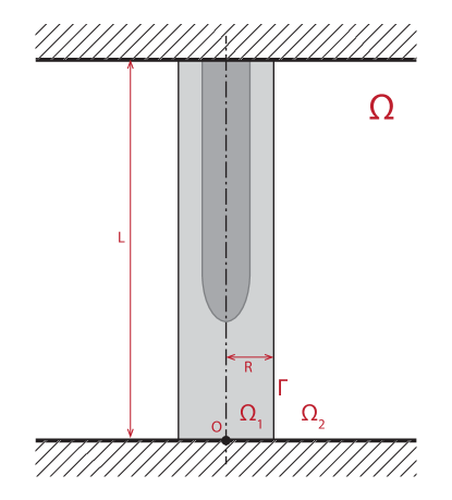
Figure 1: Geometry of the discharge considered in this work. An elongated channel propagates between two conducting electrodes. The space between these electrodes, $\Omega$ is divided into two domains: the inner domain $\Omega_{1}$ is our computational domain and contains all the space charge. The outer domain $\Omega_{2}$ extends indefinitely outwards from the external boundary of $\Omega_{1}$ and does not contain any space charge. The cylindrical surface $\Gamma$ is the common boundary between $\Omega_{1}$ and $\Omega_{2}$.

The most convenient decomposition of the domain strongly depends on the problem at hand. The decomposition we present here is suitable for elongated discharges and probably some other applications but the procedure and the highlighted ideas are not restricted to this particular scheme.

We consider the geometry sketched in figure 1, where an elongated, cylindrically symmetrical streamer propagates between two planar electrodes. With minimal changes, our scheme can be extended to more complex geometries commonly employed in streamer simulations, such as protrusion-plane, protrusion-protrusion and sphere-plane. The electrostatic potential $\phi$ satisfies the Poisson equation with appropriate boundary conditions:

$$\begin{array}[]{ccc}\Delta\phi=f&\text{in}&\Omega,\\ \phi=g&\text{on}&\partial\Omega,\end{array}$$ (1)

where $f=-q/\epsilon_{0}$, with $q$ being the charge density and $\epsilon_{0}$ the vacuum permittivity. In principle an arbitrary boundary condition, here denoted by $g$, can be applied to the upper and lower electrodes. However, to simplify our discussion we limit ourselves to the most common case where $g=0$, meaning $\phi=0$ at $z=0$ and $z=L$ (to impose a potential difference $V$ between the two electrodes we simply add $\phi_{\text{inhom}}=zV/L$ to the solution of the homogeneous problem). The domain $\Omega$ is the space between the two electrodes, formally defined as

$$\Omega=\left\{x\equiv\left(\rho,\theta,z\right)\in\mathbb{R}^{3}/0\leq\rho,0\leq\theta<2\pi,0\leq z\leq L\right\}.$$ (2)

Since our geometry is cylindrically symmetrical, we will henceforth omit the variable $\theta$ and consider the two-dimensional domain spanned by the variables $(\rho,z)$.

Our purpose is to decompose the physical domain $\Omega$ into two, which we name $\Omega_{1}$ and $\Omega_{2}$, such that $\Omega=\overline{\Omega}_{1}\cup\overline{\Omega}_{2}$ ($\overline{\Omega}_{i}$ is the closure of the set $\Omega_{i}$), $\Omega_{1}\cap\Omega_{2}=\emptyset$ and $\operatorname{supp}(f)\subset\Omega_{1}$, i.e. all the space charge is contained in $\Omega_{1}$. The inner domain $\Omega_{1}$, extending up to a given radius $R$, is our computational domain and therefore must be selected to be as narrow as possible.

Under this domain decomposition the problem (1) turns into two coupled problems:

$$\begin{array}[]{ccc}\Delta\phi_{i}=f&\text{in}&\Omega_{i},\\ \phi_{i}=0&\text{on}&\partial\Omega_{i}\setminus\Gamma,\\ \phi_{i}=\phi_{\Gamma}&\text{on}&\partial\Gamma,\end{array}$$ (3)

where $i=1,2$ and $\Gamma=\partial\Omega_{1}\cap\partial\Omega_{2}$ is the cylindrical surface at $\rho=R$ that separates the two domains.

Since at the interface $\Gamma$ both, $\phi_{1}$ and $\phi_{2}$, are equal to the boundary value $\phi_{\Gamma}$, they fulfill $\phi_{1}=\phi_{2}$. But besides this condition, in order for $\phi_{1}$ and $\phi_{2}$ to be consistent with the solution $\phi$ of the original problem (1), they must also satisfy

$$\frac{\partial\phi_{1}}{\partial\rho}=\frac{\partial\phi_{2}}{\partial\rho}\;\text{on}\;\Gamma.$$ (4)

2.2 Linearity

The linearity of the Poisson problems (3) with respect to their sources $f$ allows us to decompose the potentials as

$$\phi_{i}=\bar{\phi}_{i}[\phi_{\Gamma}]+\tilde{\phi}_{i}[f_{i}],$$ (5)

where $\bar{\phi}_{i}[\phi_{\Gamma}]$ results from the boundary values $\phi_{\Gamma}$ at the interface $\Gamma$ and $\tilde{\phi}_{i}[f_{i}]$ results from the original sources $f$ restricted to $\Omega_{i}$ (we use $[\cdot]$ to denote a functional dependence). The precise definitions read

$$\begin{array}[]{ccc}\Delta\bar{\phi}_{i}=0&\text{in}&\Omega_{i},\\ \bar{\phi}_{i}=0&\text{on}&\partial\Omega_{i}\setminus\Gamma,\\ \bar{\phi}_{i}=\phi_{\Gamma}&\text{on}&\partial\Gamma,\end{array}$$ (6)

and

$$\begin{array}[]{ccc}\Delta\tilde{\phi}_{i}=f&\text{in}&\Omega_{i},\\ \tilde{\phi}_{i}=0&\text{on}&\partial\Omega_{i}\setminus\Gamma,\\ \tilde{\phi}_{i}=0&\text{on}&\partial\Gamma.\end{array}$$ (7)

In terms of these components the flux equation (4) can be expressed as

$$\frac{\partial\bar{\phi}_{1}}{\partial\rho}\left[\phi_{\Gamma}\right]-\frac{\partial\bar{\phi}_{2}}{\partial\rho}\left[\phi_{\Gamma}\right]=-\frac{\partial\tilde{\phi}_{1}}{\partial\rho}\left[f\right]\;\text{on}\;\Gamma,$$ (8)

where on the right hand side we have made use of $\tilde{\phi}_{2}=0$, since f=0 in $\Omega_{2}$.

2.3 Expansion in orthonormal solutions of the Laplace equation

The potentials $\bar{\phi}_{i}$ in (6) are solutions of the Laplace equation in cylindrical geometry and they can be expanded using an orthogonal basis of solutions (see e.g. [19]):

$$\bar{\phi}_{1}=\sum_{m=1}^{\infty}\alpha_{m}I_{0}\left(k_{m}\rho\right)\sin\left(k_{m}z\right),$$ (9a)

$$\bar{\phi}_{2}=\sum_{m=1}^{\infty}\beta_{m}K_{0}\left(k_{m}\rho\right)\sin\left(k_{m}z\right),$$ (9b)

where $\alpha_{m}$ and $\beta_{m}$ are expansion coefficients, $k_{m}=m\pi/L$ and $I_{n}\left(x\right)$ and $K_{n}\left(x\right)$ are the modified $n$-order Bessel functions of the first and second kind respectively. Note that the set $S=\left\{\sin\left(k_{m}z\right)\right\}_{m=0}^{\infty}$ is an orthogonal basis of

$$\mathcal{L}^{2}\left(\left[0,L\right]\right)=\left\{f\mathrel{\mathop{\mathchar 58\relax}}\left[0,L\right]\mapsto\mathbb{R}\mathrel{\mathop{\mathchar 58\relax}}\int\left|f\left(z\right)\right|\text{\texttwosuperior}dz<\infty\right\},$$ (10)

therefore, $\phi_{\Gamma}$ can be expanded as:

$$\phi_{\Gamma}\left(z\right)=\sum_{m=1}^{\infty}a_{m}\sin\left(k_{m}z\right).$$ (11)

If $\phi_{\Gamma}$ is continuous and piecewise differentiable on $\left[0,L\right]$, $\phi_{\Gamma}^{\prime}\in\mathcal{L}^{2}\left(\left[0,L\right]\right)$ and $\phi_{\Gamma}$ satisfies homogeneous Dirichlet boundary conditions, then the sine series converges to $\phi_{\Gamma}$ uniformly on $\left[0,L\right]$. Note that the term with $m=0$ vanishes due to the homogeneous boundary conditions at $z=0$ and $z=L$.

The boundary conditions at $z=0$ and $z=L$ restrict the basis of solutions. Homogeneous Dirichlet boundary conditions are simpler because there is only need for sine functions. However, if we had some other boundary conditions such as homogeneous Neumann, the convenient basis should also include cosine functions to allow for non-zero values of the potential at $z=0$ and $z=L$. Nevertheless, this basis is not orthogonal and this would make things slightly more complicated.

2.4 Continuity of the normal derivative

Imposing that $\bar{\phi}_{1}=\bar{\phi_{2}}=\phi_{\Gamma}$ at $\rho=R$ we solve for $\alpha_{m}$ and $\beta_{m}$ and write (9b) as

$$\bar{\phi}_{1}=\sum_{m=1}^{\infty}a_{m}\frac{I_{0}\left(k_{m}\rho\right)}{I_{0}\left(k_{m}R\right)}\sin\left(k_{m}z\right),$$ (12a)

$$\bar{\phi}_{2}=\sum_{m=1}^{\infty}a_{m}\frac{K_{0}\left(k_{m}\rho\right)}{K_{0}\left(k_{m}R\right)}\sin\left(k_{m}z\right).$$ (12b)

Using these expressions into the equation for the normal derivatives (8) we obtain

$$\sum_{m=1}^{\infty}a_{m}k_{m}\left[\frac{I_{1}\left(k_{m}R\right)}{I_{0}\left(k_{m}R\right)}+\frac{K_{1}\left(k_{m}R\right)}{K_{0}\left(k_{m}R\right)}\right]\sin(k_{m}z)=-\left.\frac{\partial\tilde{\phi}_{1}}{\partial\rho}\right|_{\rho=R},$$ (13)

where we have made use of the identities $I_{0}^{\prime}(x)=I_{1}(x)$, $K_{0}^{\prime}(x)=-K_{1}(x)$. Using now the orthogonality of the basis $S$ we obtain equations for the coefficients $a_{m}$:

$$\frac{L}{2}k_{m}a_{m}\left[\frac{I_{1}\left(k_{m}R\right)}{I_{0}\left(k_{m}R\right)}+\frac{K_{1}\left(k_{m}R\right)}{K_{0}\left(k_{m}R\right)}\right]=-\int_{0}^{L}\operatorname{d\!}z\,\sin\left(k_{m}z\right)\left.\frac{\partial\tilde{\phi}_{1}}{\partial\rho}\right|_{\rho=R}.$$ (14)

In a space discretization based on a cartesian grid the integral in the latest expression is approximated by a finite sum with the form of a Discrete Sine Transform (DST). This leads to this final expression for the coefficients $a_{m}$

$$a_{m}=-\frac{2}{m\pi}\left[\frac{I_{1}\left(k_{m}R\right)}{I_{0}\left(k_{m}R\right)}+\frac{K_{1}\left(k_{m}R\right)}{K_{0}\left(k_{m}R\right)}\right]^{-1}\;\sum_{i=1}^{N}h\sin\left(k_{m}z_{i}\right)\left.\frac{\partial\tilde{\phi}_{1}}{\partial\rho}\right|_{\rho=R,z=z_{i}}+\mathcal{O}(h^{2}),$$ (15)

where $h$ is the grid size and $\left\{z_{i}\right\}_{i=1}^{N}$ are the solution nodes in the $z$-direction. In a discrete problem the series in (11) is also truncated above $m=N$.

2.5 Algorithm

We are now ready to detail the domain-decomposition algorithm that allows us to solve the Poisson equation in the reduced computational domain $\Omega_{1}$ with free boundary conditions:

1. Solve the Poisson equation in $\Omega_{1}$ with the source term $f$ and homogeneous Dirichlet boundary conditions at the boundary $\Gamma$. Call the result $\tilde{\phi}_{1}$.

2. Calculate the normal derivative of $\tilde{\phi}_{1}$ at $\Gamma$. Apply a DST and use expression (15) to obtain the coefficients $a_{m}$.

3. Use these coefficients to obtain the boundary values $\phi_{\Gamma}$ by means of a second DST and expression (11).

4. Solve again the Poisson equation in $\Omega_{1}$ but now use $\phi_{\Gamma}$ as inhomogeneous Dirichlet boundary condition at $\Gamma$. The result, $\phi_{1}$ is the solution of the Poisson equation with free boundary conditions.

To this algorithm we add the following remarks:

1. After obtaining the coefficients $a_{m}$ one is tempted to use (12a) together with $\phi_{1}=\bar{\phi}_{1}+\tilde{\phi}_{1}$ to avoid solving the Poisson equation a second time. However, in a grid of $M\times N$ cells this procedure takes about $MN^{2}$ operations whereas solving the Poisson equation requires only $MN\log(MN)$ or $MN$ operations.

2. The computational domain $\Omega_{1}$ has to be as narrow as possible in order to reduce the computational cost of the simulation. Of course this narrowing is limited by the constraint that $\Omega_{1}$ contains the support of the space charge density. In an electrostatic discharge the charge density typically decays smoothly away from the channel so in some cases one has to decide at which level it is safe to truncate the charge density with an acceptable error. Nevertheless, given the fast decay of the charge away from the channel, this is probably not a serious concern in most cases.

3 Tests and sample implementation

3.1 Tests

In order to test our scheme we consider now a simple setup where the Poisson equation has a closed-form solution. An example of such a configuration is a uniformly charged sphere located between two grounded, infinite planar electrodes. The electrostatic potential in this setup can be calculated by the method of images (see e.g. [19]) and equals the potential created in free space by an infinite series of spheres with alternating charges.

Suppose a sphere centred at $(\rho,z)=(0,z_{0})$ with radius $a<\min(z_{0},L-z_{0})$ and total charge $Q$. At a point with cylindrical coordinates $(\rho,z)$ the potential reads

$$\phi(\rho,z)=\phi_{0}(\rho,z)+\frac{Q}{4\pi\epsilon_{0}}\sum_{\begin{subarray}{c}k=-\infty\\ k\neq 0\end{subarray}}^{\infty}\frac{(-1)^{k}}{\left[\rho^{2}+\left(z-z_{0}-2k(L-z_{0})\right)^{2}\right]^{1/2}},$$ (16a)

with

$$\phi_{0}(\rho,z)=\frac{Q}{4\pi\epsilon_{0}}\begin{cases}\frac{1}{\left[\rho^{2}+\left(z-z_{0}\right)^{2}\right]^{1/2}}&\text{if $\rho^{2}+(z-z_{0})^{2}>a^{2}$},\\ \frac{3a^{2}-\rho^{2}-(z-z_{0})^{2}}{2a^{3}}&\text{if $\rho^{2}+(z-z_{0})^{2}\leq a^{2}$}.\end{cases}$$ (16b)

Figure 2 shows a comparison between the electric fields computed using expression (16b) and using the approach described in section 2. Here we took $a=$3\text{\,}\mathrm{m}\mathrm{m}$$, $L=$10\text{\,}\mathrm{m}\mathrm{m}$$, $Q=${10}^{13}\text{\,}\mathrm{e}$$ (e is the elementary charge), $z_{0}=L/2$. For the discretized solution we used $\Delta r=\Delta z=${10}^{-2}\text{\,}\mathrm{m}\mathrm{m}$$ and a radial extension of the computational domain $R=$5\text{\,}\mathrm{m}\mathrm{m}$$. We also include the electrostatic potential calculated by imposing homogeneous Neumann boundary conditions at the external boundary.

We see that the field calculated with the approach presented here is indistinguishable from the field from the method of images. The homogeneous Neumann conditions, on the other hand, produce an electric field that at the surface of the sphere deviates by about 15% from the other two in the worst case, i.e. with $R=$5\text{\,}\mathrm{m}\mathrm{m}$$. To investigate the convergence of the homogeneous Neumann solution we extended the computational domain by computing the field also for $R=$10\text{\,}\mathrm{m}\mathrm{m}$$ and $R=$20\text{\,}\mathrm{m}\mathrm{m}$$. As we move the external boundary away, the solution with Neumann conditions approaches our reference solution (Method of Images). Essentially, bringing the external boundary closer to the charged sphere shields the electric field before so the Neumann condition is fulfilled. As we will see, applied to streamer simulations, this leads to slightly lower values of the electric field in the streamer head and therefore less ionization.

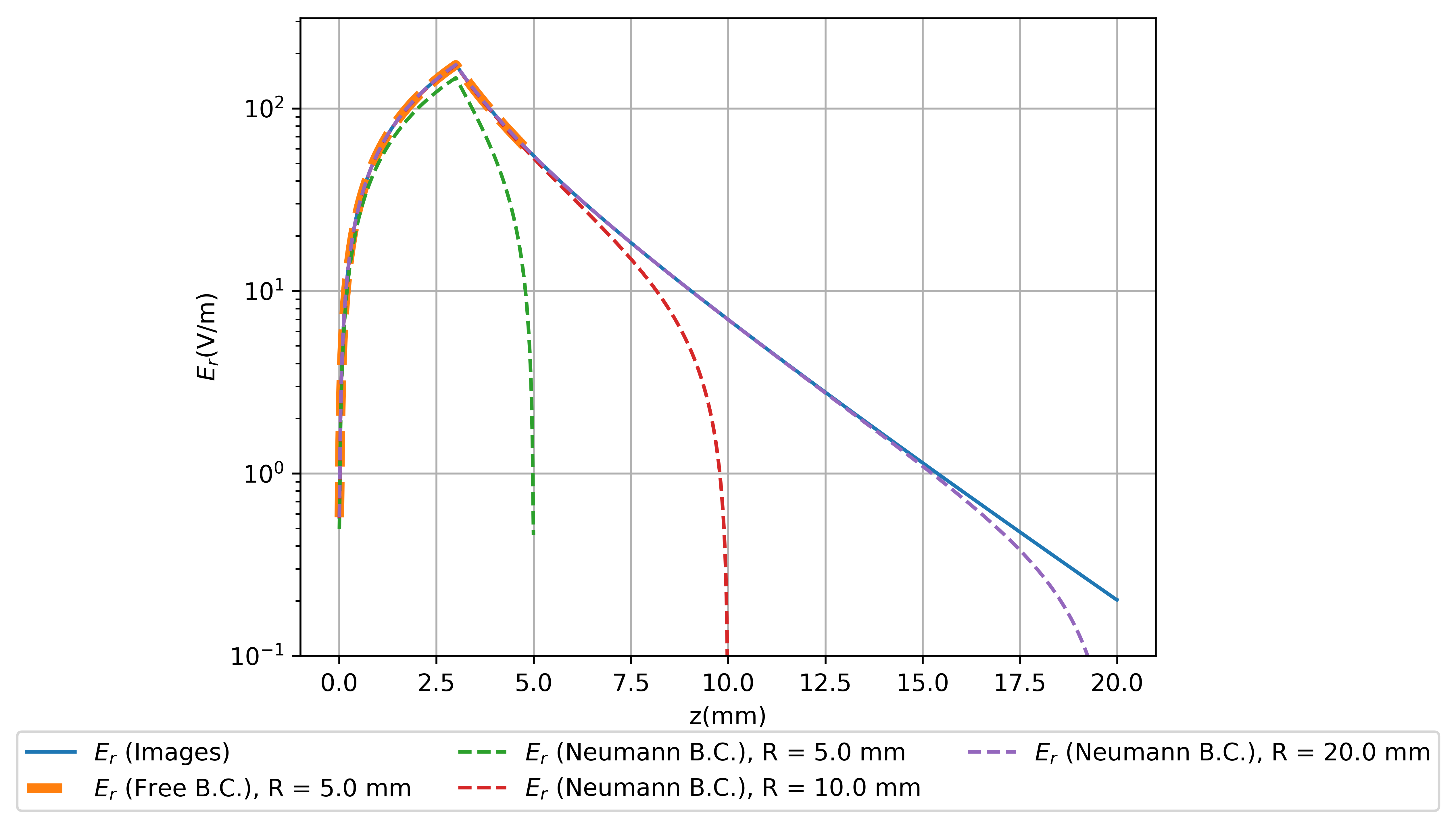
Figure 2: Comparison between electric fields created by a uniformly charged sphere between two planar infinite electrodes calculated by the approach presented in this work, by the method of images and by imposing homogeneous Neumann boundary conditions at the external boundary of the computational domain. Note the overlap between the lines corresponding to free boundary conditions and to the method of images.

3.2 Order of accuracy

We have checked that the method described above does not change the order of accuracy of the discretization of the Poisson equation by constructing a closed-form solution of the Poisson equation that satisfies homogeneous Dirichlet boundary conditions in the upper and lower electrodes. We have used the potential

$$\phi=\sin\left(\pi\frac{z}{L}\right)e^{-\frac{r^{2}}{\sigma^{2}}-\frac{\left(z-z_{0}\right)^{2}}{\sigma^{2}}},$$ (17)

whose Laplacian has the form

$$\begin{split}\Delta\phi=&\frac{1}{L^{2}\sigma^{4}}\left\{4L\pi\sigma^{2}\left(z-z_{0}\right)\cos\left(\pi\frac{z}{L}\right)+\left[\pi^{2}\sigma^{4}+L^{2}\left(-4r^{2}+6\sigma^{2}-4\left(z-z_{0}\right)^{2}\right)\right]\right\}\\ &\times\sin\left(\pi\frac{z}{L}\right)e^{-\frac{r^{2}}{\sigma^{2}}-\frac{\left(z-z_{0}\right)^{2}}{\sigma^{2}}}.\end{split}$$ (18)

Although this charge density is not strictly bounded, the contribution of charges excluded from the domain decays super-exponentially as the domain becomes wider and can thus be neglected as long as the external radius of the computational domain is significantly longer than $\sigma$.

We have solved the Poisson equation corresponding to the Laplacian (18) with $L=$1\text{\,}\mathrm{m}$$, $\sigma=$0.1\text{\,}\mathrm{m}$$ and $z_{0}=$0.5\text{\,}\mathrm{m}$$ within a cylindrical domain with a radius $R=$0.5\text{\,}\mathrm{m}$$, where we imposed free boundary conditions with the method described above. In this manner we checked that the convergence in the $\ell^{2}$-norm is of second order, the same as that of the finite difference scheme. This is as expected because $\tilde{\phi}_{1}$, its derivative in the radial direction and the Fourier coefficients (15) retain convergence of order $\mathcal{O}\left(h^{2}\right)$.

We are also interested in the convergence as we move the outer boundary. Following the example of the previous section, this time we change the radius of the sphere to 0.1 mm and the mesh spacing to $1\text{\,}\mu\mathrm{m}$. Errors are presented in Table 1, and the convergence is as expected of second order. Therefore, the decomposition method does not cause errors of order less than two.

Outer radius (mm)	$\left\|\epsilon\right\|_{2}$	$\frac{\left\|\epsilon\right\|_{2}}{\left\|\phi_{exact}\right\|_{2}}$
0.2	$5.919\text{\times}{10}^{-7}$	$5.037\text{\times}{10}^{-6}$
0.5	$4.735\text{\times}{10}^{-8}$	$3.812\text{\times}{10}^{-7}$
1	$1.227\text{\times}{10}^{-8}$	$9.838\text{\times}{10}^{-8}$

Table 1: Error obtained with change in outer radius

3.3 Sample implementation

A computer code that produces a figure similar to figure 2 is included with this work. The code is implemented in Python and to be executed it requires only the widely available scientific libraries NumPy and SciPy. To solve the discrete Poisson equation the code constructs a sparse matrix for the discrete Laplacian operator and invokes UMFPACK [20] (via SciPy) to solve the resulting linear system.

The code consists of a single file poisson_sparse_fft.py and contains the following methods:

compute_matrix: Calculates the sparse matrix for the discrete Laplacian operator in a given cartesian grid and boundary conditions.

apply_inhom_bc: Modifies the right-hand-side of the linear system in order to apply inhomogeneous Dirichlet boundary conditions.

DDM: Applies the domain decomposition method described in section 2 to solve the Poisson equation with free boundary conditions.

MOI: Calculates the electrostatic potential by means of the method of images, using (16b).

main: This is the entry-point of the code: it uses the above methods to produce the output figure.

4 Streamer simulations

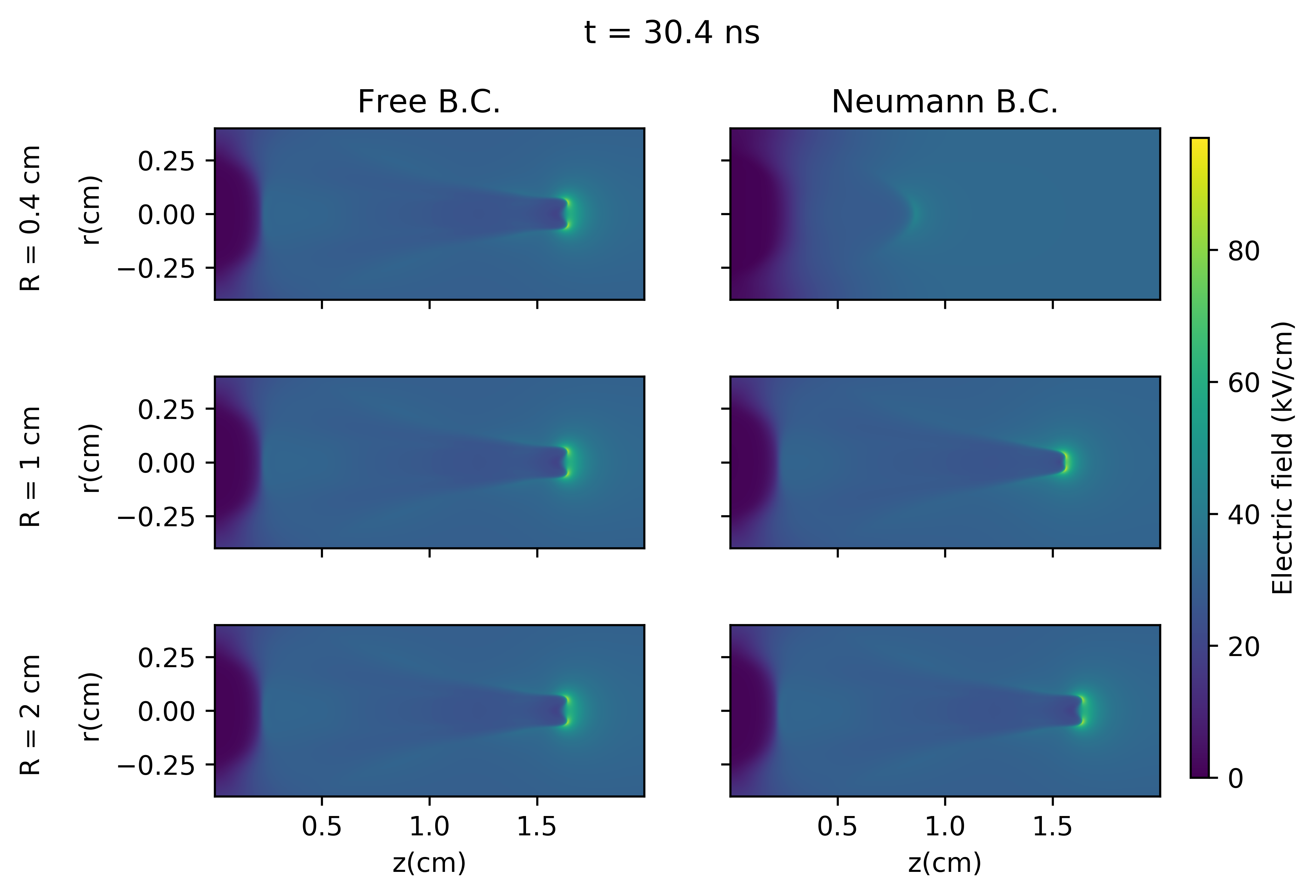
Figure 3: Streamer simulations using free boundary conditions (left column) and homogeneous Neumann boundary conditions (right column) in the external boundary of the computational domain. For each selection of the boundary conditions we show three simulations where the computational domain extends to a radius $R=$0.5\text{\,}\mathrm{c}\mathrm{m}$$ (top), $R=$1\text{\,}\mathrm{c}\mathrm{m}$$ (middle) and $R=$2\text{\,}\mathrm{c}\mathrm{m}$$ (bottom).

In elongated electric discharges, Neumann boundary conditions are often considered more appropriate than Dirichlet to be applied at $r_{max}$ because there is not a physical electrode in the radial direction, and therefore there is no reason to keep constant the potential there. The development of electric discharges is driven by long range interactions and therefore boundary conditions certainly affect the solution inside the computational domain. These effects can be reduced by enlarging the domain in the radial direction in exchange of a higher computational cost. The procedure we have described allows us to keep the boundary $r_{max}$ close to the core of the simulation without noticeable numerical effects on the electric discharge. The following simulations clearly illustrate the features mentioned.

We simulated the propagation of streamer discharges between two planar electrodes with a model that includes electron drift, impact ionization and dissociative attachment and is implemented using the CLAWPACK/PetClaw library [21, 22]. The Poisson equation is solved using the Improved Stabilized version of BiConjugate Gradient solver from the PETSc numerical library [23, 24]. For more details about the physical model see e.g. references [25, 26, 4].

We selected an inter-electrode gap of $L=$2\text{\,}\mathrm{c}\mathrm{m}$$ and a background electric field of $27\text{\,}\mathrm{k}\mathrm{V}\mathrm{/}\mathrm{c}\mathrm{m}$. The streamer is initiated by a neutral ionization seed attached to the electrode on the central axis and centred at $z=L$. The peak electron density in this seed is ${10}^{14}\text{\,}\mathrm{c}\mathrm{m}^{-3}$ and the $e$-folding length is $0.7\text{\,}\mathrm{m}\mathrm{m}$.

As we are interested in the effect of the external boundary conditions, we run simulations both with free boundary conditions, implemented as described above, and with homogeneous Neumann conditions for the electrostatic potential (as mentioned above, it is generally assumed that Neumann boundary conditions introduce slightly smaller artifacts). We also use different radii of the computational domain, $R=$0.5\text{\,}\mathrm{c}\mathrm{m}$$, $R=$1\text{\,}\mathrm{c}\mathrm{m}$$ and $R=$2\text{\,}\mathrm{c}\mathrm{m}$$. In figure 3 we show snapshots of the electric field resulting from these simulations at time $t=$30\text{\,}\mathrm{n}\mathrm{s}$$, shortly after the streamer branches in the simulations with free boundary conditions. Note however that the cylindrical symmetry of the simulations prevents proper branching. MovieS1 (available online) shows the complete evolution of the streamers.

In the plots we see that the simulations with free boundary conditions are essentially identical regardless of the lateral extension of the computational domain. The simulations with homogeneous Neumann conditions on the other hand depend artificially on the radius of the computational domain. The streamer barely develops with $R=$0.5\text{\,}\mathrm{c}\mathrm{m}$$ and only the simulation with $R=$2\text{\,}\mathrm{c}\mathrm{m}$$ reproduces accurately the branching time of the simulations with free boundary conditions. We conclude that, even in this case where the aspect ratio of the discharge is not extremely high, the computational gain from reducing the domain size (roughly a factor 4) more than compensates for the cost of solving twice the Poisson equation, resulting in an overall improvement of about a factor 2.

5 Discussion and conclusions

When they are not laterally constrained, most electrical discharges develop as elongated channels. Despite different physical conditions and ionization mechanisms this feature is common to streamers, leaders and arcs. The underlying reason for this shared property is that all these processes are affected by a Laplacian instability [27, 28], whereby small bumps in a discharge front enhance the electric field ahead and thus grow faster than the surrounding regions. This prevents the formation of wide, smooth discharges and creates branched discharge trees of many filaments [29].

Since this is the preferred shape of a discharge, it is reasonable to optimize our numerical models for elongated channels, selecting high-aspect-ratio computational domains. The method and the code that we have presented here can be used to achieve this efficiently and without losing accuracy.

We mention several possible extensions and refinements of this method. The first one, which is described in the appendix, consists in extending the free boundary conditions also to the upper and lower simulation boundaries. This can be useful for the investigation of discharges not attached to any electrode or, with appropriate modifications, attached to a single electrode.

A second extension is to adapt the method to run in parallel in several processors. If we parallelize the Poisson solver by vertically decomposing the domain, the application of the method described above requires collecting information about the initial solution around the external boundary and then performing a one-dimensional Fourier transform. The overhead of these steps is small compared to the operations required for the solution of the Poisson equation so the method can be efficiently parallelized.

Finally, one may ask about the suitability of this method for non-uniform meshes and, in particular, for adaptively refined meshes. Although the application of the method is in principle straightforward, a careful analysis is required to understand the error incurred due to a possibly coarser resolution around the boundary than around a localized charge density. This analysis, however, falls out of the scope of the present paper.

Note that although we have focused on the solution of the Poisson equation, this method can be easily generalized to other elliptic partial differential equations. This can then applied to other components of streamer simulation codes such as the speeding-up of photoionization calculations by approximating the interaction integral by combining solutions of a set of partial differential equations, as proposed in references [30, 31, 11].

Appendix A Full free boundary conditions

The focus in this paper is the implementation of free boundary conditions in the outer boundary of a discharge confined between two parallel plates but the method described above can also be extended to implement free boundary conditions in all boundaries of a simulation with cylindrical symmetry. In this appendix we describe this extension.

A.1 Domain decomposition

The method described above allows us to solve the Poisson equation in the space between two infinite, parallel planes. To build upon this procedure we decompose now the full-space domain $\Omega$ into three disjoint subdomains, which we name $\Omega_{0}$, $\Omega_{1}$ and $\Omega_{2}$ (see figure 4). We assume now that the support of the charge distribution $f$ is contained in $\Omega_{0}$ and thus arrive at the three coupled problems

$$\begin{array}[]{ccc}\Delta\phi_{0}=f&\text{in}&\Omega_{0},\\ \phi_{0}=\phi_{\Gamma_{0i}}&\text{on}&\partial\Gamma_{0i},i=1,2,\end{array}$$ (19a)

and

$$\begin{array}[]{ccc}\Delta\phi_{i}=f&\text{in}&\Omega_{i},\\ \phi_{i}=\phi_{\Gamma_{0i}}&\text{on}&\partial\Gamma_{0i},\end{array}$$ (19b)

where $i=1,2$ and $\Gamma_{0i}=\partial\Omega_{0}\cap\partial\Omega_{i}$ are the surfaces $z=0$ and $z=L$ respectively.

Since there are two interfaces, there are also two conditions for the continuity of the normal derivative:

$$\frac{\partial\phi_{0}}{\partial z}=\frac{\partial\phi_{i}}{\partial z}\;\text{on}\;\Gamma_{i},i=1,2.$$ (20)

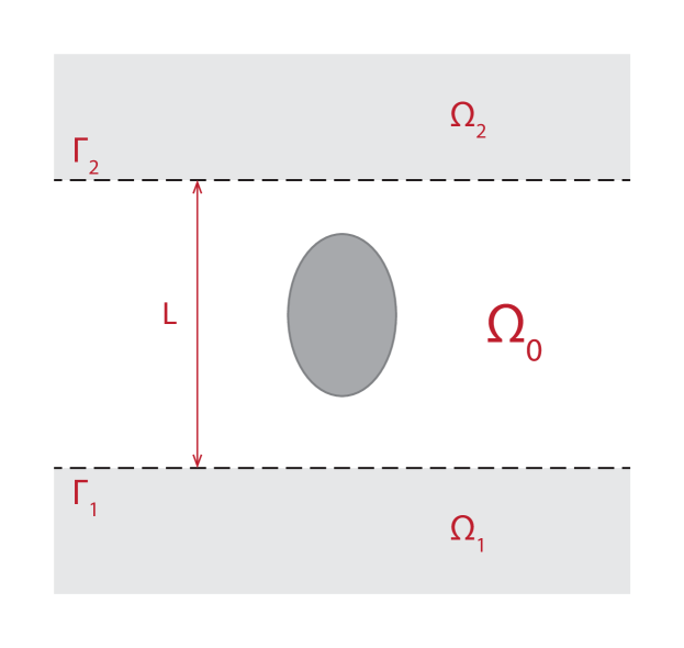
Figure 4: Geometry of the problem. $\Omega$ is divided into three subdomains: $\Omega_{0}$, $\Omega_{1}$ and $\Omega_{2}$. The three extend indefinitely outwards and the latter two also downwards and upwards respectively.

A.2 Linearity

Linearity allows us to split the problem into

$$\begin{array}[]{ccc}\Delta\bar{\phi}_{0}=0&\text{in}&\Omega_{0},\\ \bar{\phi}_{0}=\phi_{\Gamma_{0i}}&\text{on}&\partial\Gamma_{0i},i=1,2,\end{array}$$ (21a)

$$\begin{array}[]{ccc}\Delta\tilde{\phi}_{0}=f&\text{in}&\Omega_{0},\\ \tilde{\phi}_{0}=0&\text{on}&\partial\Gamma_{0i},i=1,2\end{array}$$ (21b)

and for $i=1,2$,

$$\begin{array}[]{ccc}\Delta\bar{\phi}_{i}=0&\text{in}&\Omega_{i},\\ \bar{\phi}_{i}=\phi_{\Gamma_{0i}}&\text{on}&\partial\Gamma_{0i},\end{array}$$ (22a)

$$\begin{array}[]{ccc}\Delta\tilde{\phi}_{i}=f&\text{in}&\Omega_{i},\\ \tilde{\phi}_{i}=0&\text{on}&\partial\Gamma_{0i}.\end{array}$$ (22b)

Since there is no charge outside the computational domain, $\tilde{\phi}_{i}=0$ for $i=1,2$. These equations are naturally subject to the condition that the potential vanishes at $-z,z,\rho\rightarrow\infty$.

Note now that the problem (21b) can be solved by the procedure described in the main text, since $\tilde{\phi}_{0}$ is the union of the solutions to the problems at (3).

In terms of these components, the flux equation (4) can be expressed as

$$\frac{\partial\bar{\phi}_{0}}{\partial z}\left[\phi_{\Gamma_{0i}}\right]-\frac{\partial\bar{\phi}_{i}}{\partial z}\left[\phi_{\Gamma_{0i}}\right]=-\frac{\partial\tilde{\phi}_{0}}{\partial z}\left[f\right]\;\text{on}\;\Gamma,\;\forall i.$$ (23)

A.3 Expansion in solutions of the Laplace equation

The potentials $\bar{\phi}_{i}$ in (22a) are solutions of the Laplace equation in cylindrical coordinates and they can be expanded using a set of solutions (see e.g. [19]). Since the domain is unbounded in the radial direction, instead of a series expansion we obtain an integral transform, which we can write in terms of the zero-order Hankel transform, which reads:

$$\bar{\phi}_{0}=\int_{0}^{\infty}k\operatorname{d\!}k\left[A\left(k\right)e^{kz}+B\left(k\right)e^{-kz}\right]J_{0}\left(k\rho\right),$$ (24a)

$$\bar{\phi}_{1}=\int_{0}^{\infty}k\operatorname{d\!}k\>C\left(k\right)e^{kz}J_{0}\left(k\rho\right),$$ (24b)

$$\bar{\phi}_{2}=\int_{0}^{\infty}k\operatorname{d\!}k\>D\left(k\right)e^{-kz}J_{0}\left(k\rho\right),$$ (24c)

where $J_{0}\left(x\right)$ is the zero-order Bessel function of the first kind and the functions $A,B,C,D$ weight the independent solutions to the Laplace equation. Note that, although the factor $k$ can be absorbed into these functions, it appears explicitly in order to show the Hankel transform structure.

The function $\phi_{\Gamma_{0i}}$ can also be transformed as:

$$\phi_{\Gamma_{0i}}\left(\rho\right)=\int_{0}^{\infty}k\operatorname{d\!}kE_{i}\left(k\right)J_{0}\left(k\rho\right).$$ (25)

Casting these equations in the form of a Hankel transform is important because as the Hankel transform can be inverted (it is its own inverse) we can use the fact that, subject to some regularity assumptions,

$$\int_{0}^{\infty}k\operatorname{d\!}k\>F\left(k\right)J_{0}\left(k\rho\right)=0\iff F(k)=0.$$ (26)

A.4 Continuity of the normal derivative

Imposing that $\bar{\phi}_{0}=\bar{\phi_{i}}=\phi_{\Gamma_{0i}}$ at $z=0\;\text{and}\;L,$ we solve for $A,B,C,D$ using (26) and write (24c) as

$$\bar{\phi}_{0}=\int_{0}^{\infty}\frac{k\operatorname{d\!}k}{e^{2kL}-1}\left[\left(E_{2}e^{kL}-E_{1}\right)e^{kz}+\left(-E_{2}+E_{1}e^{kL}\right)e^{-k\left(z-L\right)}\right]J_{0}\left(k\rho\right),$$ (27a)

$$\bar{\phi}_{1}=\int_{0}^{\infty}k\operatorname{d\!}k\>E_{1}e^{kz}J_{0}\left(k\rho\right),$$ (27b)

$$\bar{\phi}_{2}=\int_{0}^{\infty}k\operatorname{d\!}k\>E_{2}e^{-k\left(z-L\right)}J_{0}\left(k\rho\right).$$ (27c)

Using these expressions into the equation for the normal derivative (23) we obtain

$$\int_{0}^{\infty}\frac{2e^{kL}k^{2}\operatorname{d\!}k}{e^{2kL}-1}\left(E_{2}-E_{1}e^{kL}\right)J_{0}\left(k\rho\right)=-\left.\frac{\partial\tilde{\phi}_{0}}{\partial z}\right|_{z=0},$$ (28a)

$$\int_{0}^{\infty}\frac{e^{kL}k^{2}\operatorname{d\!}k}{e^{2kL}-1}\left(E_{2}e^{kL}-E_{1}\right)J_{0}\left(k\rho\right)=-\left.\frac{\partial\tilde{\phi}_{0}}{\partial z}\right|_{z=L}.$$ (28b)

We can obtain the coefficients $E_{1}$ and $E_{2}$ going back to the $k$-space by means of the Hankel transform:

$$E_{1}\left(k\right)=\frac{1}{2}\left(e^{-kL}I_{L}-I_{0}\right),$$ (29a)

$$E_{2}\left(k\right)=\frac{1}{2}\left(I_{L}-e^{-kL}I_{0}\right),$$ (29b)

where

$$I_{0,L}\left(k\right)=-\frac{1}{k}\int_{0}^{\infty}\rho\operatorname{d\!}\rho\left.\frac{\partial\tilde{\phi}_{0}}{\partial z}\right|_{z=0,L}J_{0}\left(k\rho\right).$$ (30)

In this expression $\tilde{\phi}_{0}$ and its normal derivative are known from the algorithm described in 2.5. Therefore we can compute $I_{0,L}$ and, using (29b) $E_{1,2}$. These functions in turn can be inserted in (25) to yield the boundary condition to impose on $\Gamma_{1,2}$.

Supplementary Data

The Supplementary Data include a movie (MovieS1) showing the development of several streamer discharges within domains of different radial extent as described in section 4. Among a total of six cases, three of them show the development of the discharge for Poisson’s equation subject to Neumann boundary conditions whereas the remaining three correspond to the solution of Poisson’s equation with free radial boundary conditions. Figure 3 is a frame extracted from this movie.

References

- [1] J. R. Dwyer, M. A. Uman, The physics of lightning, Phys. Rep.534 (2014) 147. doi:10.1016/j.physrep.2013.09.004.
- [2] U. Ebert, C. Montijn, T. M. P. Briels, W. Hundsdorfer, B. Meulenbroek, A. Rocco, E. M. van Veldhuizen, The multiscale nature of streamers, Plasma Sour. Sci. Technol. 15 (2006) S118. arXiv:physics/0604023, doi:10.1088/0963-0252/15/2/S14.
- [3] N. Liu, V. P. Pasko, Effects of photoionization on similarity properties of streamers at various pressures in air, J. Phys. D 39 (2006) 327. doi:10.1088/0022-3727/39/2/013.
- [4] A. Luque, U. Ebert, Density models for streamer discharges: Beyond cylindrical symmetry and homogeneous media, J. Comput. Phys. 231 (2012) 904. doi:10.1016/j.jcp.2011.04.019.
- [5] N. Liu, J. R. Dwyer, H. C. Stenbaek-Nielsen, M. G. McHarg, Sprite streamer initiation from natural mesospheric structures, Nature Communications 6 (2015) 7540. doi:10.1038/ncomms8540.
- [6] J. Qin, V. P. Pasko, Dynamics of sprite streamers in varying air density, Geophys. Res. Lett. 42 (2015) 2031. doi:10.1002/2015GL063269.
- [7] J. Teunissen, U. Ebert, Afivo: a framework for quadtree/octree AMR with shared-memory parallelization and geometric multigrid methodsarXiv:1701.04329.
- [8] N. Y. Babaeva, G. V. Naidis, Two-dimensional modelling of positive streamer dynamics in non-uniform electric fields in air, J. Phys. D 29 (1996) 2423. doi:10.1088/0022-3727/29/9/029.
- [9] N. Y. Babaeva, G. V. Naidis, Modeling of streamer propagation, in: E. M. van Veldhuizen (Ed.), Electrical discharges for environmental purposes: fundamentals and applications, Nova Science, New York, United States, 2000.
- [10] N. Liu, V. P. Pasko, Effects of photoionization on propagation and branching of positive and negative streamers in sprites, J. Geophys. Res. (Space Phys) 109 (2004) A04301. doi:10.1029/2003JA010064.
- [11] A. Bourdon, V. P. Pasko, N. Y. Liu, S. Célestin, P. Ségur, E. Marode, Efficient models for photoionization produced by non-thermal gas discharges in air based on radiative transfer and the Helmholtz equations, Plasma Sour. Sci. Technol. 16 (2007) 656. doi:10.1088/0963-0252/16/3/026.
- [12] C. R. Anderson, A method of local corrections for computing the velocity field due to a distribution of vortex blobs, J. Comput. Phys. 62, 111 (1986). doi:10.1016/0021-9991(86)90102-6.
- [13] R. J. James, The solution of Poisson’s equation for isolated source distributions, J. Comput. Phys. 25 (1977) 71-93. doi:10.1016/0021-9991(77)90013-4.
- [14] Gregory T. Balls, Phillip Colella, A Finite Difference Domain Decomposition Methods Using Local Corrections for the Solution of Poisson’s Equation, J. Comput. Phys. 180, 25-53 (2002). doi:10.1006/jcph.2002.7068.
- [15] Mads Mølholm Hejlesen, Johannes Tophøj Rasmussen, Philippe Chatelain Jens Honoré Walther, A high order solver for the unbounded Poisson equation, J. Comput. Phys. 252 (1) (2013) 458-467. doi:10.1016/j.jcp.2013.05.050.
- [16] Christopher R. Anderson, High order expanding domain methods for the solution of Poisson’s equation in infinite domains, J. Comput. Phys. 314 (2016) 194-205. doi:10.1016/j.jcp.2016.02.074.
-
[17]
C. R. Anderson, Domain decomposition
techniques and the solution of poissons’s equation in infinite domains, in:
T. Chan, R. Glowinski, J. Périaux, O. Widlund (Eds.), Domain Decomposition
Methods, Proceedings in Applied Mathematics, SIAM, 1989.
URL http://www.ddm.org/DD02/Proc-2.php - [18] A. Bayliss, M. Gunzburger, E. Turkel, Boundary conditions for the numerical solution of elliptic equations in exterior regions, SIAM J. App. Math 42 (2) (1982) 430–451. doi:10.1137/0142032.
- [19] J. Jackson, Classical electrodynamics, John Wiley and sons, New York, USA, 1975.
-
[20]
T. A. Davis, Algorithm 832:
Umfpack v4.3—an unsymmetric-pattern multifrontal method, ACM Trans. Math.
Softw. 30 (2) (2004) 196–199.
doi:10.1145/992200.992206.
URL http://doi.acm.org/10.1145/992200.992206 - [21] R. LeVeque, Finite Volume Methods for Hyperbolic Problems, Cambridge Texts in Applied Mathematics, Cambridge University Press, 2002.
-
[22]
A. Alghamdi, A. Ahmadia, D. I. Ketcheson, M. G. Knepley, K. T. Mandli,
L. Dalcin, Petclaw:
A scalable parallel nonlinear wave propagation solver for python, in:
Proceedings of the 19th High Performance Computing Symposia, HPC ’11, Society
for Computer Simulation International, San Diego, CA, USA, 2011, pp. 96–103.
URL http://dl.acm.org/citation.cfm?id=2048577.2048590 -
[23]
S. Balay, S. Abhyankar, M. F. Adams, J. Brown, P. Brune, K. Buschelman,
L. Dalcin, V. Eijkhout, W. D. Gropp, D. Kaushik, M. G. Knepley, L. C.
McInnes, K. Rupp, B. F. Smith, S. Zampini, H. Zhang, H. Zhang,
PETSc Web page,
http://www.mcs.anl.gov/petsc (2016).
URL http://www.mcs.anl.gov/petsc -
[24]
S. Balay, S. Abhyankar, M. F. Adams, J. Brown, P. Brune, K. Buschelman,
L. Dalcin, V. Eijkhout, W. D. Gropp, D. Kaushik, M. G. Knepley, L. C.
McInnes, K. Rupp, B. F. Smith, S. Zampini, H. Zhang, H. Zhang,
PETSc users manual, Tech. Rep.
ANL-95/11 - Revision 3.7, Argonne National Laboratory (2016).
URL http://www.mcs.anl.gov/petsc - [25] C. Montijn, W. Hundsdorfer, U. Ebert, An adaptive grid refinement strategy for the simulation of negative streamers, J. Comput. Phys. 219 (2006) 801. arXiv:physics/0603070, doi:10.1016/j.jcp.2006.04.017.
- [26] U. Ebert, S. Nijdam, C. Li, A. Luque, T. Briels, E. van Veldhuizen, Review of recent results on streamer discharges and discussion of their relevance for sprites and lightning, J. Geophys. Res. (Space Phys) 115 (2010) A00E43. arXiv:1002.0070, doi:10.1029/2009JA014867.
- [27] M. Arrayás, U. Ebert, W. Hundsdorfer, Spontaneous Branching of Anode-Directed Streamers between Planar Electrodes, Phys. Rev. Lett. 88 (17) (2002) 174502. arXiv:nlin/0111043, doi:10.1103/PhysRevLett.88.174502.
- [28] G. Derks, U. Ebert, B. Meulenbroek, Laplacian Instability of Planar Streamer Ionization Fronts—An Example of Pulled Front Analysis, Journal of NonLinear Science 18 (2008) 551. doi:10.1007/s00332-008-9023-0.
- [29] A. Luque, U. Ebert, Growing discharge trees with self-consistent charge transport: the collective dynamics of streamers, New Journal of Physics 16 (1) (2014) 013039. arXiv:1307.2378, doi:10.1088/1367-2630/16/1/013039.
- [30] P. Ségur, A. Bourdon, E. Marode, D. Bessieres, J. H. Paillol, The use of an improved Eddington approximation to facilitate the calculation of photoionization in streamer discharges, Plasma Sour. Sci. Technol. 15 (2006) 648. doi:10.1088/0963-0252/15/4/009.
- [31] A. Luque, U. Ebert, C. Montijn, W. Hundsdorfer, Photoionization in negative streamers: Fast computations and two propagation modes, Appl. Phys. Lett. 90 (8) (2007) 081501. arXiv:physics/0609247, doi:10.1063/1.2435934.