Seasonal Effects on Honey Bee Population Dynamics: a Nonautonomous System of Difference Equations

Abstract

The honey bees play a role of unquestioned relevance in nature and the comprehension of the mechanisms affecting their population dynamic is of fundamental importance. As experimentally documented, the proper development of a colony is related to the nest temperature, whose value is maintained around the optimal value if the colony population is sufficiently large. Then, the environmental temperature, the way in which this influence the nest temperature and the colony population size, are variables closely linked to each other and deserve to be taken into account in a model that aims to describe the population dynamics. In the present study, as first step, the continuous-time autonomous system proposed by Khoury, Myerscoug and Barron (KMB) in 2011 was approximated by means a Nonstandard finite difference (NSFD) scheme in order to obtain a set of autonomous difference equations. Subsequently, with the aim to introduce the seasonal effects, a nonautonomous version (NAKMB) was proposed and formulated in discrete-time domain via a NSFD scheme, by introducing a time–-dependent formulation for the queen bee laying rate and the recruitment rate coefficients. By means the phase-plane analysis was possible to deduce that, with an appropriate choice of the parameters, the NAKMB model admits both a limit cycle at nonzero population size and an equilibrium point marking the colony collapse, depending on the initial population size.

1 Introduction

The honey bees are perhaps the most studied insects because their pollinating activities have a fundamental impact on the whole ecosystem. The growing attention to the safeguard of honey bees requires to deep understand the mechanisms that impact on the life of a colony. In order to rigorously describe the population dynamics of a colony and the role played by the surrounding environment, the mathematical modeling could be important to address the problem.

The honey bee colonies are composed by three castes: $20$-$40$ thousand workers, a queen and zero to few thousand drones [24]. The drone bee is a male and his main function is to be ready to fertilize a receptive queen, that is the unique responsible for laying eggs and for this reason is the parent of the whole colony. The worker bees are infertile and their energies are completely dedicated to the survival of the colony, by serving many roles during their lifetime: colony maintenance, brood rearing tasks, defense and foraging, among the main roles. A complete discussion about the roles of the worker bees can be found in [13]. For the purposes of this paper, it is useful to classify the work of the bees in two categories, according to the level of risk to which they are subjected: hive bees and foragers. The firsts live in a protected environment, the seconds are exposed to the external climatic conditions and are constantly life-threatening. The model proposed by Khoury, Myerscoug and Barron in 2011 [16] (cited in the present work as KMB model) describes a demographic model to explore the process of colony failure, by discussing the effect of different death rates of forager bees on colony growth. The model forecasts a threshold forager death rate $m^{*}$ such that if $m>m^{*}$ the colony is doomed to failure. The model proposed by Brown in 2013 [3] introduces a nonzero death rate also for hive bees, knowingly neglected in [16]. In both models the authors study a system of autonomous differential equations: none of the parameters explicitly depends on time.

Nevertheless, the seasonal effects are of a fundamental importance and deserve to be considered so that the model can describe the population dynamics as realistically as possible. The seasons are marked by changes in weather, in particular the temperature is one of the most impacting factors regulating the life cycle of all animals. In this paper were taken into account only the effects related to the annual variations (seasonal), neglecting the circadian ones, also important as discussed, i.e., in [9]. Seasonal effects have been investigated by Russell, Barron and Harris in 2013 [27], with a detailed dynamic flow model using a commercial software (Stella, isee system - version 8.0) that takes into account the influence of the seasonality on death rates and food availability. Their work report also a complete review of the other models taking into account seasonal effects.

In this paper is first proposed a discrete-time version of the KMB model, by taking advantage of the Nonstandard Finite Difference Scheme (NSFD) [19]. The NSFD introduces some rules ensuring a finite difference scheme without the instabilities sometimes introduced by the other discretization methods. In scientific literature there are many applications of the NSFD scheme, each showing the robustness and flexibility of the method (see, i.e., [19, 20, 21, 22, 10]). After, the seasonal effects were evaluated by introducing a new formulation for the queen laying rate and the recruitment functions. The problem is first formulated in continuous-time domain by means a system of two nonlinear nonautonomous differential equations and after, applying the NSFD rules, in discrete-time domain.

2 Definitions and preliminaries

In this section some basic definitions will be given, about the concept of stability of a dynamical system, with particular regard to discrete-time formulation.

2.1 Autonomous dynamical systems

2.1.1 Continuous-time

A general $n$-dimensional autonomous continuous-time dynamical system is defined by the equation

$$\left\{\begin{array}[]{l}\frac{d\xi(t)}{dt}=F(\xi(t),k)\\ \\ \xi(t_{0})=\xi_{0}\in\mathbb{R}^{n}_{+},\\ \end{array}\right.$$ (4)

with $F:\mathbb{R}^{n}\longrightarrow\mathbb{R}^{n}$ is supposed to be differentiable in $\mathbb{R}^{n}_{+}$ and constitutes a vector field, $\xi=\xi(t):[0,+\infty)\longrightarrow\mathbb{R}^{n}$ is the state at time $t$, with initial condition $\xi_{0}\in\mathbb{R}^{n}_{+}$, and $k=(k_{1},k_{2},\ldots)$ represents the system parameters. If $F$ is globally Lipschitz, then there exists a unique solution $\xi(t)$ for all $t\geq t_{0}$, hence the (4) defines a dynamical system on $\mathbb{R}^{n}$. In general $F$ could be linear or nonlinear respect to $\xi$; in this paper only nonlinear systems will be discussed.

Definition 2.1.

For a system defined with (4), a steady-state solution is a point $\tilde{\xi}\in\mathbb{R}^{n}$ satisfying the relation:

$$F(\tilde{\xi})=0.$$ (5)

In the continuation of the text the set $\Gamma_{c}=\{\tilde{\xi}|f(\tilde{\xi})=0,\,\tilde{\xi}\in\mathbb{R}^{n}\}$ will indicate the set of steady-states solutions.

In order to evaluate the stability of the steady-state solutions of the nonlinear system, a linearization around each equilibrium point is required, through the calculation of the Jacobian matrix, indicated with $J_{F}$, and its eigenvalues, indicated with $\lambda$.

Definition 2.2.

Let $\sigma(J_{F})$ the set of eigenvalues of $J_{F}$, a steady-state $\tilde{\xi}\in\mathbb{R}^{n}$ for which $J_{F}$ has no eigenvalues with zero real parts, named hyperbolic steady-states, is [18]:

• asymptotically stable if and only if $\Re\lambda<0$, for all $\lambda\in\sigma(J_{F})$,

• unstable if and only if $\Re\lambda>0$, for all $\lambda\in\sigma(J_{F})$.

This criterion does not apply for nonhyperbolic steady-states, characterized by one or more eigenvalues with $\Re\lambda=0$.

The correspondence between the behavior of the nonlinear equations and the linearized version is ensured by the Hartman–Grobman theorem.

Theorem 2.1 (Hartman–Grobman).

If $\tilde{\xi}$ is a hyperbolic equilibrium of $d\xi(t)/dt=F(\xi(t))$, then there is a neighborhood of $\tilde{\xi}$ in which $F$ is topologically equivalent to the linear vector field $d\xi(t)/dt=J_{F}(\tilde{\xi})\xi$.

2.1.2 Discrete-time

In case of an autonomous discrete-time model, the continuous variable $t$ must be replaced by $t_{0},t_{1},\ldots,t_{k}$, with $t_{k}-t_{k-1}=\Delta t$, in which $\Delta t$ is the constant time-step; the variable $\xi(t)$ must take discrete values $\xi_{n}$. Then, the differential equation becomes a difference equation.

Let $f:\mathbb{R}^{n}\longrightarrow\mathbb{R}^{n}$, consider a sequence $\{\xi_{n}\}_{n=0}^{\infty}$: it can be defined by a mapping $\leavevmode\nobreak\ \Lambda:\mathbb{R}^{n}\times\mathbb{R}^{n}\longrightarrow\mathbb{R}^{n}$ of the form $H(\xi_{n+1},\xi_{n})$. In some cases, is possible that $\xi_{n+1}$ is given explicitly in terms of $\xi_{n}$:

$$\xi_{n+1}=\Phi(\xi_{n},k),$$ (6)

where $\Phi:A\subseteq\mathbb{R}^{n}\longrightarrow\mathbb{R}^{n}$ and $k=(k_{1},k_{2},\ldots)$ represents the system parameters.

Definition 2.3.

A steady-state (or fixed point) $\tilde{\xi}_{n}\in\mathbb{R}^{n}$ of (6) respects the following conditions:

$$\Phi(\tilde{\xi}_{n})=\tilde{\xi}_{n}.$$ (7)

Likewise to the continuous case, also in discrete case it is useful to indicate with $\Gamma_{d}=\{\tilde{\xi}_{n}|\Phi(\tilde{\xi}_{n})=0,\,\tilde{\xi}_{n}\in\mathbb{R}^{n}\}$ the set of steady-states.

Definition 2.4.

Let $\Phi\in C^{1}$, $J_{\Phi}$ its $n\times n$ Jacobian matrix and $\sigma(J_{\Phi})$ the set of the Jacobian eigenvalues, a theorem (see i.e., [7]) ensures that a steady-state $\tilde{\xi}_{n}\in\mathbb{R}^{n}$ is:

• locally asymptotically stable $\iff$ $\Re\lambda<1$, $\forall\,\lambda\in\sigma(J_{\Phi})$: this point is an attractor;

• unstable $\iff$ $\Re\lambda>1$, $\forall\lambda\in\sigma(J_{\Phi})$: this point is a repeller;

• no conclusions on stability if $\Re\lambda>1$ for some $\lambda\in\sigma(J_{\Phi})$.

Definition 2.5.

The finite difference method is called elementary stable if for all $\Delta t>0$, the stability properties of each $\tilde{\xi}_{n}\in\Gamma_{d}$ are the same of each $\tilde{\xi}\in\Gamma_{c}$.

Let $\tilde{J}_{\Phi}:=J_{\Phi}(\tilde{\xi}_{n})$, in two dimensional systems the characteristic polynomial of the Jacobian can be written as:

$$\lambda^{2}-\lambda\operatorname{tr}(\tilde{J}_{\Phi})+\det(\tilde{J}_{\Phi}).$$ (8)

In order to have $\Re\lambda<1$ for all $\lambda\in\sigma(J_{\Phi})$, the Jury condition [15] states that:

$$|\operatorname{tr}(\tilde{J}_{\Phi})|<1+\det(\tilde{J}_{\Phi})<2.$$ (9)

Therefore, this criterion establishes that exists a necessary and sufficient condition to guarantee the asymptotic stability of the steady-state solutions.

2.2 Nonautonomous dynamical systems and the Poincaré map

Definition 2.6.

If the vector field $F$ of (4) depends explicitly on $t$, the system of equations is called nonautonomous.

Definition 2.7.

In case of a nonautonomous dynamical system, if there exists a $\tau>0$ such that $F(\xi,t)=F(\xi,t+\tau)$ for all $\xi\in\mathbb{R}^{n},\,t\in\mathbb{R}$, the system is said time-periodic with period $\tau$.

A such $\tau$-periodic dynamical system can be converted into a $(n+1)$-order autonomous dynamical system by adding an equation [25]:

$$\left\{\begin{array}[]{l}\frac{d\xi(t)}{dt}=F(\xi(t),\theta\tau/2\pi,k)\\ \\ \frac{d\theta(t)}{dt}=\frac{2\pi}{\tau}\\ \\ \xi(t_{0})=\xi_{0}\in\mathbb{R}^{n}_{+},\,\theta(t_{0})=2\pi t_{0}/\tau.\\ \end{array}\right.$$ (15)

In such a way the problem is formulated in the $\mathbb{R}^{n}\times S^{1}$ toroidal phase space, where $S:=[0,2\pi)$. If $\theta$ is substituted with $\theta+2\pi m$ for $m\in\mathbb{Z}$, then the system is unchanged. In this space, the planes identified by $\theta=2\pi m$ coincide with $\theta=0$, which is a section for a Poincaré sequence [14].

3 Rules to built a numerically stable finite difference scheme

The numerical integration of ordinary differential equations using traditional methods could produce different solutions from those of the original ODE [23, 10, 5]. In particular, using a discretization step-size larger than some relevant time scale, is possible to obtain solutions that may not reflect the dynamics of the original system [23]. To overcome this problem, Ronald Mickens, in 1989, suggested what is known as the Nonstandard Finite Difference (NSFD) method [19], based on the concept of Dynamic Consistency.

Definition 3.1.

Let a first-order autonomous ODE and given $U$ its set of properties, the correspondent difference equation is dynamically consistent with the ODE if it respects the same set of properties: stability, bifurcations and eventually chaotic behavior of the original differential equation [1].

Definition 3.2.

A finite difference method is defined a NSFD scheme if at least one of the following conditions is satisfied [21]:

1. Nonlinear terms must be replaced by nonlocal discrete representations, i.e.,

   $$\xi^{2}\longrightarrow\xi_{n}\xi_{n+1}.$$

2. Denominator functions for the discrete representation must be nontrivial. The following replacement is then required:

   $$\Delta t\longrightarrow\phi(\Delta t)+O(\Delta t^{2}),$$

   where $\phi(\Delta t)$ is such that $0<\phi(\Delta t)<1$, for all $\Delta t>0$.

Remark.

The NSFD scheme incorporates the principle of Dynamical Consistency.

Other important rules to build discretization are:

• the order of the discrete derivative should be equal to the order of the corresponding derivatives of the differential equation;

• special conditions that hold for the solutions of the differential equations should also hold for the solutions of the finite difference scheme;

• the scheme should not introduce spurious solutions.

An important characteristic of dynamical systems, especially in those of biological interest, is that all solutions must remain nonnegative in order to maintain the problem well-posed, from biological and mathematical points of view.

Definition 3.3.

A method that respects the NSFD rules and preserves the solution’s positivity is called Positive and Elementary Stable Nonstandard (PESN) method.

By applying these expedients, the discrete scheme will comply with the physical properties of the differential equations, without any restriction on the step size $\Delta t$.

4 Hive bees vs foragers population: the KMB model

In this section the continuous-time model proposed in 2011 by Khoury, Myerscoug and Barron (KMB) is reported and briefly described; after, a discrete-time version is proposed.

4.1 Continuous-time model

The KMB model is based on hypothesis that a colony of honey bees is schematizable as the sum of $h$ bees working in the hive and $f$ foragers bees working outside the hive, with a total number of workers $N=h+f$. The system of differential equations proposed by the authors is:

$$\left\{\begin{array}[]{l}\frac{dh(t)}{dt}=L\frac{h(t)+f(t)}{w+h(t)+f(t)}-h(t)\bigg{(}\alpha-\sigma\frac{f(t)}{h(t)+f(t)}\bigg{)}\\ \\ \frac{df(t)}{dt}=h(t)\bigg{(}\alpha-\sigma\frac{f(t)}{h(t)+f(t)}\bigg{)}-mf(t)\\ \\ h(0)\geq 0,\,f(0)\geq 0,\\ \end{array}\right.$$ (16)

where the parameter $L$ is the maximum queen laying rate, $w$ represents the brood mortality, $\sigma$ is the social inhibition and $\alpha$ is the maximum rate at which hive bees will become foragers. In the first differential equation of (16), the sign of the right term depends upon the balance between a positive contribute, whose magnitude is related to the eclosion rate, and a negative term, named by the authors in the manuscript recruitment function, due to the hive bees recruited as foragers. The recruitment function is a balance between a term that favors the transition to foragers and another that inhibits hive bees from transitioning to foragers; with a such formulation, if the foragers number is high the inhibition term prevents a further growing of $f$.
Since it is not the purpose of this work to analyze the KMB model in all its details, the interested reader may find an exhaustive analysis in [16].

4.2 Discrete-time model

The differential equation (16) can be discretized by following the rules listed in Section 3. The obtained difference equations are:

$$\left\{\begin{array}[]{l}\frac{h_{n+1}-h_{n}}{\phi(\Delta t)}=L\frac{h_{n}+f_{n}}{w+h_{n}+f_{n}}-\alpha h_{n+1}+\sigma\frac{f_{n}h_{n}}{h_{n}+f_{n}}\\ \\ \frac{f_{n+1}-f_{n}}{\phi(\Delta t)}=h_{n}\bigg{(}\alpha-\sigma\frac{f_{n+1}}{h_{n}+f_{n}}\bigg{)}-mf_{n+1}\\ \\ h_{0}\geq 0,f_{0}\geq 0.\\ \end{array}\right.$$ (17)

That can be explicated respect to $h_{n+1}$ and $f_{n+1}$ as follows:

$$\left\{\begin{array}[]{l}h_{n+1}=\Phi_{1}(h_{n},f_{n})\\ \\ f_{n+1}=\Phi_{2}(h_{n},f_{n})\\ \\ h_{0}\geq 0,f_{0}\geq 0,\\ \end{array}\right.$$ (18)

in which

$$\left\{\begin{array}[]{l}\Phi_{1}(h_{n},f_{n})=\bigg{(}h_{n}\bigg{(}1+\frac{\sigma\phi(\Delta t)f_{n}}{h_{n}+f_{n}}\bigg{)}+L\phi(\Delta t)\bigg{(}1-\frac{w}{w+h_{n}+f_{n}}\bigg{)}\bigg{)}\frac{1}{1+\alpha\phi(\Delta t)}\\ \\ \Phi_{2}(h_{n},f_{n})=\frac{\big{(}f_{n}+h_{n}\big{)}\big{(}f_{n}+\alpha\phi(\Delta t)h_{n}\big{)}}{\big{(}1+m\phi(\Delta t)\big{)}f_{n}+\big{(}1+(m+\sigma)\phi(\Delta t)\big{)}h_{n}}\\ \\ h_{0}\geq 0,f_{0}\geq 0.\\ \end{array}\right.$$ (19)

To find the steady-states of (19) the condition (7) must be satisfied:

$$\left\{\begin{array}[]{l}\Phi_{1}(h_{n},f_{n})=h_{n}\\ \\ \Phi_{2}(h_{n},f_{n})=f_{n}\\ \\ h_{0}\geq 0,f_{0}\geq 0.\\ \end{array}\right.$$ (20)

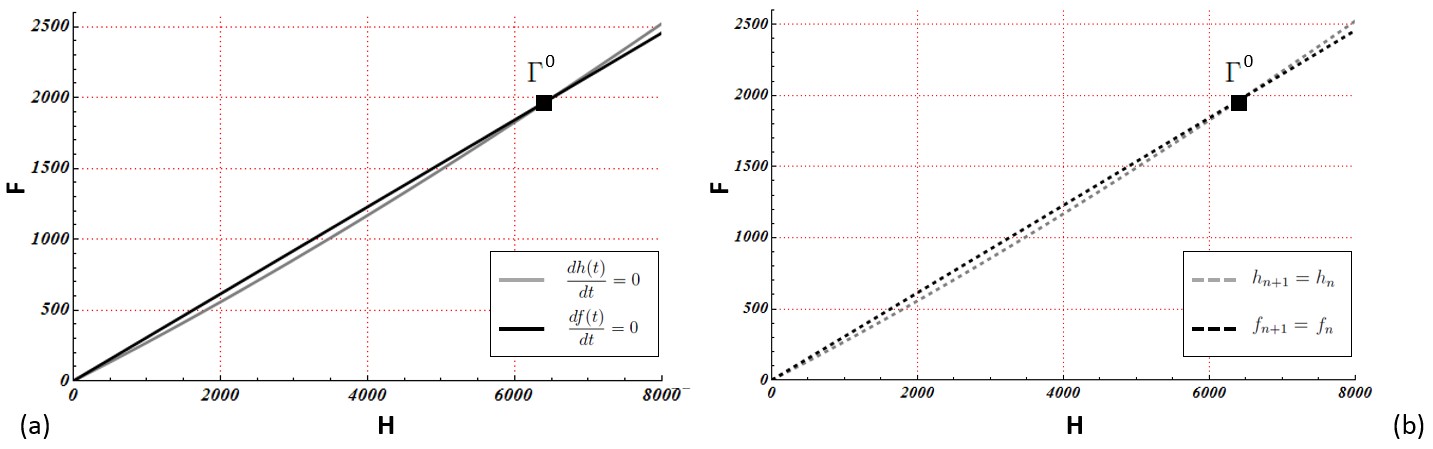
Figure 1: Comparison between phase-plane diagrams for continuous-time and discrete-time KMB models. (a) Zero-growth isoclines for system (16) are represented as gray ($dh(t)/dt=0$) and black ($df(t)/dt=0$) lines. (b) Zero-growth isoclines of system (17): black dotted line for the first equation and gray dotted line for the second equation. The steady-state is identified by the letter $\Gamma^{0}$. The values assigned at each parameter are: $L=2000$, $\alpha=0.25$, $\sigma=0.75$, $w=27000$ and $m=0.24$. The values assigned to the discretization parameters are: $\Delta t=0.1$ and $q=0.5$.

The nontrivial form of $\phi(\Delta t)$, requested by the second rule of Definition 3.2, is given by the following expression [21]:

$$\phi(\Delta t)=\frac{1-e^{-q\Delta t}}{q}.$$ (21)

Introducing $\Omega=\bigcup_{\tilde{\xi}\in\Gamma_{d}}\sigma(\tilde{J})$, the optimal value of $q$ must respect the condition

$$q\geq\max_{\Omega}\Big{\{}\frac{\lambda^{2}}{2|\Re(\lambda)|}\Big{\}}\,\,\,\rm if\,\,\,\Re(\lambda)\neq 0\,\,for\,\,\,\lambda\in\Omega.$$ (22)

By assuming $L=2000$, $\alpha=0.25$, $\sigma=0.75$, $w=27000$ and $m=0.24$, the same values adopted in [16], the zero-growth isoclines in continuous and in discrete cases are represented respectively in Figure 1a and b. In both cases, they intersect in the point $\Gamma^{0}=(H^{0},F^{0})\simeq(6470,1988)$: this means that $\Gamma^{0}$ constitutes an equilibrium point of both the systems (16) and (17).

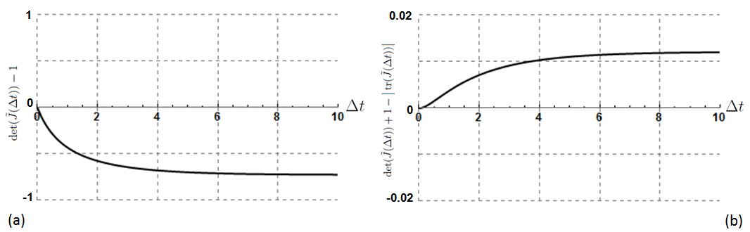
Figure 2: Jury condition validation for NSFD scheme. (a) Plot of $\det(\tilde{J}(\Delta t))-1$ versus the time step $\Delta t$. (b) Plot of $\det(\tilde{J}(\Delta t))+1-\big{|}\operatorname{tr}(\tilde{J}(\Delta t))\big{|}$ versus $\Delta t$.

To evaluate the stability of $\Gamma_{0}$ in continuous-time, the definition 2.2 must be taken into account. In particular, the set of eigenvalues calculated in point $\Gamma^{0}$ is $\sigma(J_{F}(H^{0},F^{0}))\simeq\{-0.83,-0.014\}$; since they are both negatives, is possible to conclude that $\Gamma^{0}$ is asymptotically stable. The magnitude of the eigenvalues implies a choice of $q\geq 0.41$, then a $q=0.5$ was used for the numerical calculations described in the following sections.

In the discrete-time case, in order to evaluate the stability of $\Gamma_{0}$, is sufficient to consider the inequality (9) and rewrite it making explicit the dependence on $\Delta t$ in order to control if the step size affects or not the stability of $\Gamma^{0}$:

$$\det(\tilde{J}(\Delta t))-1<0,$$ (23)

$$\det(\tilde{J}(\Delta t))+1-\big{|}\operatorname{tr}(\tilde{J}(\Delta t))\big{|}>0.$$ (24)

The Figure 2a and Figure 2b show the left terms of inequalities expressed respectively in (23) and in (24): it is possible to note that both the inequalities (23) and (24) are respected up to $\Delta t=10$, then, in this time-step interval, $\Gamma^{0}$ is asymptotically stable as found in continuous case.

5 NAKMB: the proposed nonautonomous KMB model

In this section a nonautonomous version of the KMB model is proposed, in which the seasonal effects are investigated by introducing a time-dependent formulation for some of the parameters involved in KMB model. Also, differently from the original KMB model, in addition to the foragers bees death rate, a nonzero death rate for hive bees was assumed in order to reproduce a possible depopulation related to inadequate nutrition, brood disease or to the presence of Varroa mites and viruses, among the main factors [3].

5.1 Time-dependent parameters

A healthy colony of honey bees regulates the temperature of the nest $T^{N}$ using heating and cooling systems [4], to compensate for the variations of the environmental temperature $T^{E}$. In [11, 12] was highlighted that, in order to grant the proper rearing of brood, an optimal value for the nest temperature $T^{O}$ exists, comprised in the narrow range of $32$-$36\,^{\circ}C$, with a mean of $34.5\,^{\circ}C$. In case of necessity, in order to cool the hive during the warmer months, the worker bees start fanning, evaporate water by tongue lashing or spread droplets of water on the brood [2]; conversely, to heat the nest, the bees form a cluster clinging to each other. The role of the temperature, that of the nest in direct way and the environmental one in a roundabout way, is then of the utmost importance and it deserves to be taken into account in a model that aims to describe how the population evolves in time.

Below, the fundamental hypotheses at the base of the NAKMB model are discussed and the mathematical formulation is given:

• The queen laying rate $L$ is influenced by the nest temperature. This assumption is justified by the evidence that a low deposition rate is linked to a $T^{N}$ substantially greater or smaller than $T^{O}$ [6]. To reproduce this behavior the proposed formula is:

  $$L(t)=\frac{L_{0}(\Gamma/2)^{2}}{(T^{N}(t)-T^{O})^{2}+(\Gamma/2)^{2}},$$ (25)

  where $L_{0}$ is the maximum laying rate. The function defined in (25) is a Lorentzian curve characterized by a width $\Gamma$, multiplied by a factor such that, if $T^{N}=T^{O}$, then $L_{max}=L_{0}$. The $\Gamma$ represents the ability to withstand deviations of the nest temperature from the optimal value.

• The nest temperature is maintained around the optimal value if the total number of individuals in a colony $N$ overcomes a critical threshold $N^{T}$; if the number of individuals falls below that threshold the colony may fail to incubate brood or maintain the optimum temperature in the nest [26, 17]. To capture this effect the following formulation is proposed:

  $$T^{N}(t)=\frac{T^{E}(t)}{1+\big{(}\frac{f+h}{N^{T}}\big{)}^{2}}+\frac{T^{O}}{1+\big{(}\frac{N^{T}}{f+h}\big{)}^{2}}$$ (26)

• The environmental temperature $T^{E}$ is supposed to have sinusoidal behavior with annual periodicity:

  $$T^{E}(t)=\theta_{0}+\theta_{1}\sin(\Omega t)+\theta_{2}\cos(\Omega t),$$ (27)

  in which $\Omega=2\pi/\tau$, $\tau$ is the period. The coefficients $\theta_{0}$, $\theta_{1}$ and $\theta_{2}$ can be estimated by least-square fitting of the environmental temperature measured, for example, by a weather station.

• The recruitment function, due to hive bees recruited as foragers, unlike the KMB model, is supposed to be influenced by the season. To meet this need, it can be multiplied by a coefficient

  $$\eta(t)=\eta_{0}+\eta_{1}\sin(\Omega t)+\eta_{2}\cos(\Omega t).$$ (28)

  In particular, since the foraging activity stops during the winter and is maximum during the spring, $\eta(t)$ must have zero-phase delay respect to $T^{E}(t)$ (maxima and minima coinciding) and respect $0\leq\eta(t)\leq 1$. To satisfy these two requirements the coefficients in (28) must be linked to $\theta_{1}$ and $\theta_{2}$ as follows (see the proof in the Appendix):

  $$\eta_{0}=\frac{1}{2},\,\,\eta_{1}=-\frac{\theta_{1}\theta_{2}}{2\big{(}\theta_{1}^{2}+\theta_{2}^{2}\big{)}}\sqrt{1+\bigg{(}\frac{\theta_{1}}{\theta_{2}}\bigg{)}^{2}},\,\,\eta_{2}=-\frac{\theta_{2}^{2}}{2\big{(}\theta_{1}^{2}+\theta_{2}^{2}\big{)}}\sqrt{1+\bigg{(}\frac{\theta_{1}}{\theta_{2}}\bigg{)}^{2}}$$ (29)

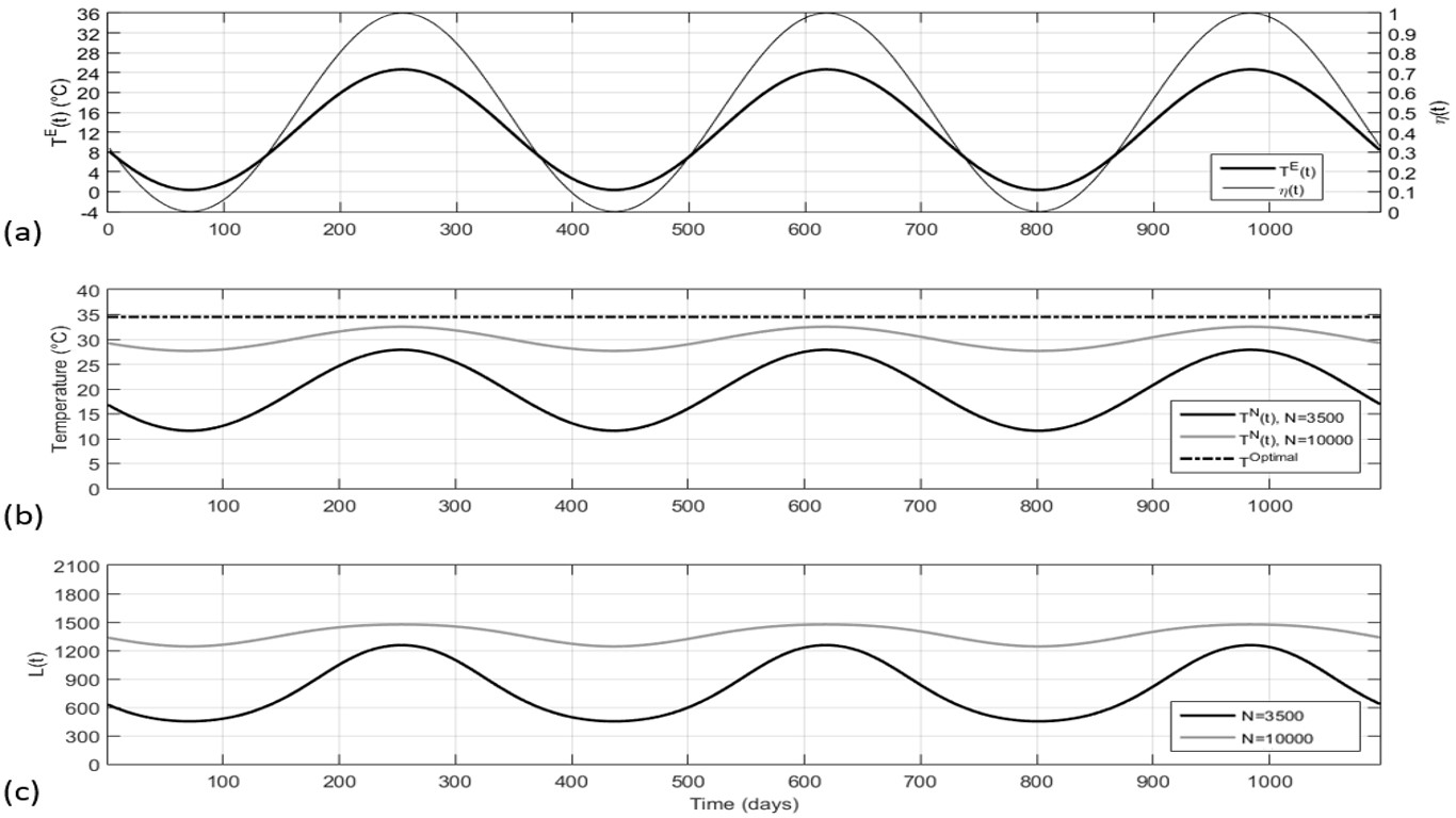
Figure 3: Temporal evolution of the environmental temperature $T^{E}(t)$, recruiting function coefficient $\eta(t)$, nest temperature $T^{N}(t)$ and queen laying rate $L(t)$ over a period of 2 years. (a) $T^{E}(t)$ of (27) with $\theta_{0}=12.51\,^{\circ}{\rm C}$, $\theta_{1}=-11.41\,^{\circ}{\rm C}$, $\theta_{2}=-4.16\,^{\circ}{\rm C}$ and $\Omega=2\pi/\tau$, with period $\tau=365$ days (thick line); $\eta(t)$ of (28) with $\eta_{0}=0.5$, $\eta_{1}=-0.47$ and $\eta_{2}=-0.17$ (thin line). (b) $T^{N}(t)$ of (26) for $N_{0}=3500$ (black) and $N_{0}=10000$ individuals (gray) with $N^{T}=5000$ individuals; $T^{O}=34.5\,^{\circ}{\rm C}$ (black dashed line). (c) $L(t)$ of (25) for $N_{0}=h_{0}+f_{0}=3500$ (black) and $N_{0}=10000$ (gray), with $T^{O}=34.5\,^{\circ}{\rm C}$ and $\Gamma=30$.

In Figures 3a, b and c are shown respectively the temporal evolutions of $T^{E}(t)$, $\eta(t)$, $T^{N}(t)$ and $L(t)$ over a period of 2 years, keeping fixed the number of individuals of each population ($h=h_{0}$, $f=f_{0}$ and $N=N_{0}=h_{0}+f_{0}$). In particular, in Figure 3a is shown the $T^{E}(t)$, whose coefficients $\theta_{0}$, $\theta_{1}$ and $\theta_{2}$ were evaluated by nonlinear least-square fitting of the annual variation of temperature registered by the meteorological station located in Osnago, Italy (lat: $45.68^{\circ}$, long: $9.38^{\circ}$) during the year 2012 [29]. Superimposed on $T^{E}(t)$ there is $\eta(t)$, whose coefficients $\eta_{0}$, $\eta_{1}$ and $\eta_{2}$ are calculated by using (29). By setting the threshold population at $5000$ individuals [28], the nest temperature is calculated and shown in Figure 3b for two values of the total populations $N=3500$ and $N=10000$, respectively below and above the critical threshold. In Figure 3c is represented the queen laying rate for $N=3500$ and $N=10000$.

From the Figure 3b, it is possible to see that the nest temperature is maintained close to the optimal value if the population is greater than the critical threshold, otherwise is greatly influenced by the environmental temperature. Consequently, being $L(t)$ dependent on $T^{N}(t)$, and being $T^{N}(t)$ linked to the total number of individuals in a colony, results that $L(t)$ is sensitively influenced by the number of individuals in a colony.

5.2 Continuous-time NAKMB model

The system of autonomous nonlinear differential equations at the base of the KMB model is modified as follows:

$$\left\{\begin{array}[]{l}\frac{dh(t)}{dt}=L(t)\frac{h(t)+f(t)}{w+h(t)+f(t)}-\eta(t)h(t)\bigg{(}\alpha-\sigma\frac{f(t)}{h(t)+f(t)}\bigg{)}-\mu h(t)\\ \\ \frac{df(t)}{dt}=\eta(t)h(t)\bigg{(}\alpha-\sigma\frac{f(t)}{h(t)+f(t)}\bigg{)}-mf(t)\\ \\ h(0)\geq 0,\,f(0)\geq 0,\\ \end{array}\right.$$ (30)

where $L(t)$ and $\eta(t)$ are expressed respectively in (25) and in (28). In the right term of the first equation $\mu$ represents the death rate factor afflicting the hive bees. Since the laying rate and the recruiting function coefficients were assumed explicitly depending on time, the model defined in (30) is nonautonomous.

5.3 Discrete-time NAKMB model: a nonstandard formulation

The system (30) is now formulated in discrete-time domain by taking advantage of the NSFD scheme. The proposed formulation is:

$$\left\{\begin{array}[]{l}\frac{h_{n+1}-h_{n}}{\phi(\Delta t)}=L_{n}\frac{h_{n}+f_{n}}{w+h_{n}+f_{n}}-\alpha\eta_{n}h_{n+1}+\sigma\eta_{n}\frac{f_{n}h_{n}}{h_{n}+f_{n}}\\ \\ \frac{f_{n+1}-f_{n}}{\phi(\Delta t)}=\eta_{n}h_{n}\bigg{(}\alpha-\sigma\frac{f_{n+1}}{h_{n}+f_{n}}\bigg{)}-mf_{n+1}\\ \\ h_{0}\geq 0,f_{0}\geq 0,\\ \end{array}\right.$$ (31)

in which

$$L_{n}=\frac{L_{0}(\Gamma/2)^{2}}{(T^{N}_{n}-T^{O})^{2}+(\Gamma/2)^{2}},$$ (32)

$$T^{N}_{n}=\frac{T^{E}_{n}}{1+\big{(}\frac{f_{n}+h_{n}}{N^{T}}\big{)}^{2}}+\frac{T^{O}}{1+\big{(}\frac{N^{T}}{f_{n}+h_{n}}\big{)}^{2}},$$ (33)

$$T^{E}_{n}=\theta_{0}+\theta_{1}\sin(\Omega n)+\theta_{2}\cos(\Omega n),$$ (34)

$$\eta_{n}=\eta_{0}+\eta_{1}\sin(\Omega n)+\eta_{2}\cos(\Omega n).$$ (35)

With simple algebraic manipulation, the explicit form of $h_{n+1}$ and $f_{n+1}$ is obtained:

$$\left\{\begin{array}[]{l}h_{n+1}=\bigg{(}h_{n}+L_{n}\frac{h_{n}+f_{n}}{w+h_{n}+f_{n}}+\sigma\phi(\Delta t)\frac{\eta_{n}f_{n}h_{n}}{f_{n}+h_{n}}\bigg{)}\big{(}1+\phi(\Delta t)(\mu+\alpha\eta_{n})\big{)}^{-1}\\ \\ f_{n+1}=\frac{\big{(}f_{n}+\alpha\phi(\Delta t)\eta_{n}h_{n}\big{)}}{\sigma\phi(\Delta t)\big{(}1+m\phi(\Delta t)\big{)}\eta_{n}h_{n}}\\ \\ h_{0}\geq 0,f_{0}\geq 0.\\ \end{array}\right.$$ (36)

The choice of the NSFD method has left the chance to customize the discretization of (30) in order to verify the positivity condition for $h_{n+1}$ and $f_{n+1}$. In fact, since all the parameters are nonnegative, the condition $h_{n+1},f_{n+1}\geq 0$ is verified for all $n\in\mathbb{Z}^{+}$, then the NAKMB respects the PESN criterion formalized in Definition 3.3.

5.4 Phase-plane analysis

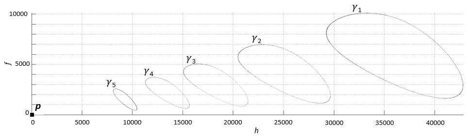
Figure 4: Phase-plane of $h$ and $f$ expressed in (36). The trajectories start from $2000\leq h_{0}\leq 20000$, $500\leq f_{0}\leq 8000$. The steady states, labelled with $\gamma_{1}\div\gamma_{5}$, and the equilibrium point at $(h,f)=(0,0)$, labelled with $p$ and highlighted with a black square, are obtained with different values of $\mu$: $0$, $0.015$, $0.03$, $0.045$, $0.06$ and $0.07$. The other parameters are: $L_{0}=2000$, $\alpha=0.25$, $\sigma=0.75$, $\omega=10000$, $m=0.24$, $N^{T}=5000$, $T^{O}=34.5\,^{\circ}{\rm C}$, $\theta_{0}=12.51\,^{\circ}{\rm C}$, $\theta_{1}=-11.41\,^{\circ}{\rm C}$, $\theta_{2}=-4.16\,^{\circ}{\rm C}$, $\Gamma=30$ and $\Omega=2\pi/\tau$, with period $\tau=365$ days. Number of iterations: $3\cdot 10^{4}$.

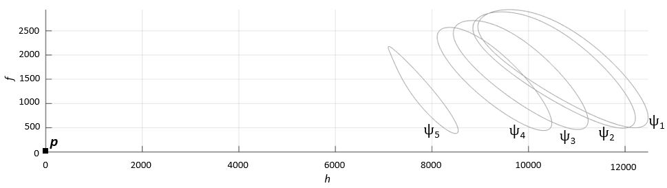
Figure 5: Phase-plane of $h$ and $f$ expressed in (36). The trajectories start from $2000\leq h_{0}\leq 20000$ and $500\leq f_{0}\leq 8000$ and increase with a step of $500$ individuals. The steady states, labelled with $\psi_{1}\div\psi_{5}$, and the equilibrium point at $(h,f)=(0,0)$, labelled with $p$ and highlighted by a black square, were obtained with different values of $\Gamma$: $100$, $60$, $35$, $30$ and $25$. The number of iterations and the values attributed to the parameters are the same used for computation of Figure 4, except for $\mu=0.06$.

The phase-plane of the discrete NAKMB model is calculated, by assuming the initial conditions $2000\leq h_{0}\leq 20000$, $500\leq f_{0}\leq 8000$ with an increment of $500$ individuals. The main purpose is to evaluate the effects of the parameters $\mu$ and $\Gamma$ on the asymptotical behavior of the system.

In Figure 4 the phase-plane of NAKMB model is represented for different values of the parameter $\mu$: $0$, $0.015$, $0.03$, $0.045$, $0.06$ and $0.07$. It is possible to recognize five closed loops, labelled with $\gamma_{1}$-$\gamma_{5}$ and an equilibrium point labelled with $p$, located at $(h,f)=(0,0)$ and highlighted by a black square. The closed loops $\gamma_{1}$, $\gamma_{2}$ and $\gamma_{3}$, classifiable as limit cycles, appear respectively assuming $\mu=0,\,0.015,\,0.03$; by choosing $\mu=0.045,\,0.06$ arise respectively the limit cycles $\gamma_{4}$ and $\gamma_{5}$ and the equilibrium point $p$; $\mu=0.07$ leads the system to have only the equilibrium point $p$. With an accurate analysis it was possible to verify that there exists a threshold value $\tilde{\mu}\simeq 0.038$ above which the system exhibits the two aforementioned asymptotic behaviors: depending on the initial conditions, the population can settle in a limit cycle or definitely decline; similarly, it is possible to show that assuming $\mu>\tilde{\mu}^{\prime}\simeq 0.066$ the system goes toward the equilibrium point $p$, regardless to the initial conditions. The autonomous model studied by Brown [3], in which is also considered $\mu\neq 0$, a critical threshold has been established at $\tilde{\mu}^{\prime}_{B}=0.12234969$ above which occurs the collapse of the population, by assuming a constant laying rate $L=1500$. Then, in NAKMB model, unlike in the autonomous Brown’s model, values of $\tilde{\mu}^{\prime}\leq\mu\leq\tilde{\mu}^{\prime}_{B}$ lead to the collapse of the colony. By looking at the Figure 4 it is also remarkable that the range of population in which are enclosed the limit cycles decreases by increasing the hive bees death rate $\mu$, as it is reasonable to be.

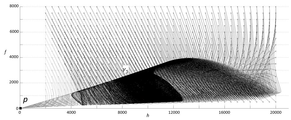
Figure 6: Phase-portrait of $h$ and $f$ expressed in (36) using the same parameters values used for computation of phase-plane in Figure 4 and $\mu=0.06$. The trajectories start from the initial points $2000\leq h_{0}\leq 20000$, $500\leq f_{0}\leq 8000$ and increase with a step of $500$ individuals. Number of iterations: $3\cdot 10^{4}$. The trajectories ending in $p$ are colored in gray and the ones ending in limit cycle $\gamma_{5}$ in black.

By fixing $\mu=0.06$, as in [3], the phase-plane of NAKMB model is calculated and represented in Figure 5 for different values of the parameter $\Gamma$: $100$, $60$, $35$, $30$ and $25$. The limit cycles $\psi_{1}$ and $\psi_{2}$ appear respectively assuming $\Gamma=100$ and $60$; the limit cycles $\psi_{3}$, $\psi_{4}$ and $\psi_{5}$, together with the equilibrium point $p$ characterized by $(h,f)=(0,0)$, appear assuming respectively $\Gamma=35,\,30$ and $25$. A detailed analysis showed that the threshold between these two behaviors is $\tilde{\Gamma}\simeq 39.5$. Similarly, it exists a second threshold $\tilde{\Gamma}^{\prime}\simeq 25.9$, so that if $\Gamma<\tilde{\Gamma}^{\prime}$ is got only the final state $p$; for this reason, the trajectory calculated assuming $\Gamma=25$ leads to $p$. This means that the larger is $\Gamma$, the better is the ability of a colony to survive to large variations of the nest temperature; smaller values lead towards a collapse of the colony. Then, an appropriate value of $\Gamma$, presumably in the range $\tilde{\Gamma}^{\prime}<\Gamma<\tilde{\Gamma}$, must be chosen in order to have two possible asymptotic states depending on the initial conditions: a limit cycle whose populations $h,\,f$ settle around ecologically plausible values and an equilibrium point representing the collapse of the colony.

In order to delineate the geometry of the basins of attraction, characterized by the set of initial conditions leading to a certain attractor, the phase portrait of (36) is calculated and represented in Figure 6, by fixing $\mu=0.06$ and $\Gamma=30$. The trajectories colored in gray are those driving the system to the collapse and the black trajectories lead to the limit cycle $\gamma_{5}$. It is easily verifiable that the two basins of attraction are separated by a straight line of equation $f(h)\simeq-1.8462h+9915$.

5.5 Toroidal phase-space representation

The temporal evolution of the NAKMB dynamical system through the phase-portrait of Figure 6 is rather complicated to be visually interpreted, since the trajectories intersect between them. The NAKMB model is, in fact, a nonautonomous model, in which the parameters $L(t)$ and $\eta(t)$ are $\tau$-periodic, then $L(t)=L(t+\tau)$ and $\eta(t)=\eta(t+\tau)$. In discrete domain, the periodicity condition corresponds to $L_{n}=L_{n+\nu}$ and $\eta_{n}=\eta_{n+\nu}$, in which $\nu=2\pi/\Omega$ is the period. Following the approach of (15), the behavior of the system of (36) can be investigated by introducing the angular variable $\theta$ so that replacing $\theta+2\pi m$ for $\theta$, $m\in\mathbb{Z}^{+}$, the system is unchanged.

A particularly suitable alternative to visualize and analyze the trajectories of periodic nonautonomous dynamical systems is given by the toroidal phase-space [14]. As introduced in Subsection 2.2, it allows an expeditious computation of the Poincaré map. The steps carried out to construct this representation are the following:

• Let $D_{0}$ the domain composed by the initial conditions and $D_{1}$ the rectangular domain enclosing the trajectories starting from $D_{0}$ for all $t$, or $n$ in discrete case ($D_{0}\subseteq D_{1}$). Suppose that $D_{1}$ is defined by $h_{a}\leq h\leq h_{b},\,f_{a}\leq f\leq f_{b}$, the new coordinates are calculated as follows:

  $$h^{\prime}=\frac{h-h_{a}}{h_{b}-h_{a}},\,\,f^{\prime}=\frac{f-f_{a}}{f_{b}-f_{a}},$$ (37)

  in which $h_{b}\neq h_{a}$ and $f_{b}\neq f_{a}$. A such transformation ensures $0\leq h^{\prime}\leq 1$ and $0\leq f^{\prime}\leq 1$.

• $h^{\prime}$-$f^{\prime}$ phase-plane is mapped into a $h^{*}$-$f^{*}$ plane by applying the diametrical transformation [14]:

  $$h^{*}=\frac{h^{\prime}}{\sqrt{1+r^{2}}},\,\,f^{*}=\frac{f^{\prime}}{\sqrt{1+r^{2}}},$$ (38)

  in which

  $$r=\sqrt{h^{\prime 2}+f^{\prime 2}}.$$ (39)

  This projection allows visualizing the whole phase-plane in a circumference of unitary radius.

Although the step I is not strictly required, with $h,f$ varying in the range $0$-$10^{4}$ individuals, the diametrical projection applied directly to $h$ and $f$ would have led to trajectories squeezed around the outer surface of the manifold $\mathbb{R}^{n}\times S^{1}$; the transformation performed in step I allows to distribute the trajectories in a larger portion of the manifold to improve the visualization.

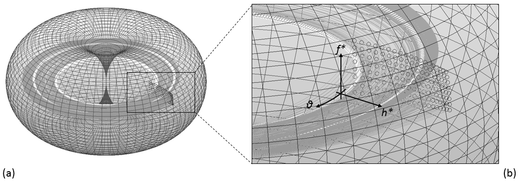
Figure 7: (a) Toroidal phase-space of the discrete NAKMB model of (36). (b) Zoom on the initial conditions, represented by black circles. The trajectories are represented in gray far from equilibrium and in white approaching to the equilibrium. The torus has unitary major and minor radii.

The toroidal phase-space is shown in Figure 7a adopting the same parameter values used to compute the Figure 6. The orbits start from the points indicated with the black circles located at $\theta=0$ and back after $2\pi m$, $m\in\mathbb{Z^{+}}$; the trajectories are colored in gray far from equilibrium and in white approaching to the equilibrium. The inner white closed path corresponds to the equilibrium point p characterized by $(h,f)=(0,0)$ in the standard phase-plane, and the outer one to the limit cycle $\gamma_{5}$.

The toroidal phase-space computation facilitates the extraction of the Poincaré map since it represents a section of the torus at a particular value of $\theta$, which is a disc of unitary radius. By fixing $\theta=\pi/2$ the Poincaré map of Figure 8 is obtained; note that only the quadrant $h^{*},f^{*}\geq 0$ is represented. The equilibrium point p and the limit cycle $\gamma_{5}$ are highlighted respectively by a square and a circle. By looking at the zoomed window of Figure 8, it is possible to note the progressive densification of the points approaching $\gamma_{5}$, as well as in phase-portrait of Figure 6 there is a densification of the intersecting paths approaching $\gamma_{5}$.

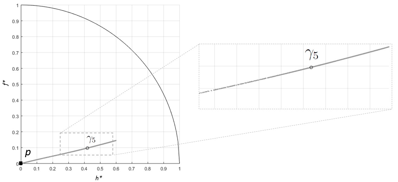
Figure 8: Poincaré map extracted as a slice at $\theta=\pi/2$ of the torus in Figure 7; only the quadrant $h^{*},f^{*}\geq 0$ is represented.

6 Conclusions

In this paper the continuous-time model proposed by Khoury et al. [16] (KMB) has been considered and formulated in discrete-time domain by adopting the Nonstandard Finite Difference (NSFD) scheme. As shown by the numerical simulations, the NSFD scheme well reproduces the behavior of the continous-time KMB model, in terms of steady-states and their stability properties.

Subsequently, a nonautonomous version of the KMB model was proposed (NAKMB), in which the seasonal effects were introduced by means a time-dependent formulation for the queen laying rate and the eclosion rate coefficient. In particular, the formulation proposed for the queen laying rate was meant to reproduce the experimental evidence that a reduced number of individuals in a colony, below a critical threshold, can hardly be able to maintain the optimum temperature in the nest, especially in the colder periods, and this could lead the entire colony toward the collapse. Taking advantages of the NSFD scheme, the NAKMB model was studied via a numerical approach in standard phase-plane and in toroidal phase-space. The system showed a sensitive dependence of the steady-states on parameters $\mu$ and $\Gamma$, respectively the hive bees death rate and the parameter introduced in the present study representing the ability of a colony to bear large variations of the nest temperature from the optimal value. In particular, small values of $\mu$ lead the population toward a limit cycle regardless of the initial conditions; by increasing $\mu$ the colony can experience a collapse or stabilizes in a limit cycle depending on the initial population; high values of $\mu$ bring the system toward the collapse, regardless of the initial population. The same three scenarios are obtained by varying $\Gamma$ from high to low values. An interesting feature of the NAKMB model is that, by assuming a moderate death rate for the foragers bees ($m=0.24$) and with an appropriate choice of the parameters, it admits two steady-states; unlike the KMB model that predicts only one equilibrium point at nonzero populations, regardless of the initial population. This features of the NAKMB model seems to be reasonable since a colony counting a number of individuals below the critical threshold encounter more difficulties to develop respect to a large colony and its collapse is a possible scenario.

Appendix A Recruiting function coefficient

The formula proposed for the recruiting function coefficient is:

$$\eta(t)=\eta_{0}+\eta_{1}\sin(\Omega t)+\eta_{2}\cos(\Omega t).$$ (40)

In this section the explicit formulation of $\eta_{0}$, $\eta_{1}$ and $\eta_{2}$ coefficients is derived. The requisites that $\eta(t)$ must respect are:

• Zero-phase delay respect to $T^{E}(t)$ of (27).

  Since

  $$\frac{dT^{E}(t)}{dt}=\Omega\big{(}\theta_{1}\cos(\Omega t)-\theta_{2}\sin(\Omega t)\big{)},$$ (41)

  for the extreme points of $T^{E}(t)$:

  $$\frac{dT^{E}(t)}{dt}=0\,\,\iff t=\hat{t}=\frac{1}{\Omega}\bigg{(}\arctan\bigg{(}\frac{\theta_{1}}{\theta_{2}}\bigg{)}+k\pi\bigg{)},\,\,k\in\mathbb{Z}.$$ (42)

  Similarly, for the extreme points of $\eta(t)$:

  $$\frac{d\eta^{E}(t)}{dt}=0\,\,\iff t=\tilde{t}=\frac{1}{\Omega}\bigg{(}\arctan\bigg{(}\frac{\eta_{1}}{\eta_{2}}\bigg{)}+k\pi\bigg{)},\,\,k\in\mathbb{Z}.$$ (43)

  In order to have zero-phase delay between $\eta(t)$ and $T^{E}(t)$, is required that $\hat{t}=\tilde{t}$, then the relation

  $$\eta_{1}\theta_{2}=\eta_{2}\theta_{1}$$ (44)

  must be respected.

  After a simple algebraic manipulation, the second derivative becomes:

  $$\frac{d^{2}\eta(t)}{dt^{2}}\bigg{|}_{t=\tilde{t}}=(-1)^{k}\frac{\eta_{1}\Omega^{2}\theta_{2}}{\theta_{1}}\bigg{(}1+\bigg{(}\frac{\theta_{1}}{\theta_{2}}\bigg{)}^{2}\bigg{)}^{1/2}.$$ (45)

  By looking at (45), it is possible to conclude that if $k$ is even, then $\tilde{t}$ is a relative minimum; if $k$ is odd, then $\tilde{t}$ is a maximum.

• $0\leq\eta(t)\leq 1$.

  From (44), $\eta_{2}=\eta_{1}\theta_{2}/\theta_{1}$ may be substituted in (40). Then, the coefficients $\eta_{0}$ and $\eta_{1}$ can be found by solving the system:

  $$\left\{\begin{array}[]{l}\eta_{0}+\eta_{1}\bigg{(}\sin(\Omega t)+\frac{\theta_{2}}{\theta_{1}}\cos(\Omega t)\eta(t)\bigg{)}=1,\,\,\forall t\in S^{M}\\ \eta_{0}+\eta_{1}\bigg{(}\sin(\Omega t)+\frac{\theta_{2}}{\theta_{1}}\cos(\Omega t)\eta(t)\bigg{)}=0,\,\,\forall t\in S^{m},\\ \end{array}\right.$$ (46)

  where $S^{M}$ is the set of the relative maximum and $S^{m}$ of the relative minimum. The solutions of (46) are:

  $$\eta_{0}=\frac{1}{2},\,\,\eta_{1}=-\frac{\theta_{1}\theta_{2}}{2\big{(}\theta_{1}^{2}+\theta_{2}^{2}\big{)}}\sqrt{1+\bigg{(}\frac{\theta_{1}}{\theta_{2}}\bigg{)}^{2}},$$ (47)

  then,

  $$\eta_{2}=-\frac{\theta_{2}^{2}}{2\big{(}\theta_{1}^{2}+\theta_{2}^{2}\big{)}}\sqrt{1+\bigg{(}\frac{\theta_{1}}{T^{b}}\bigg{)}^{2}}.$$ (48)

References

- [1] H. Al–Kahby, F. Dannan, and S. Elaydi, Non-standard discretization methods for some biological models, in R.E. Mickens (Editor), Applications of nonstandard finite difference schemes, World Scientific, Singapore, 2000, pp. 155–180.
- [2] M. A. Becher, H. Hildenbrandt, C. K. Hemelrijk, and R. F. A. Moritz, Brood temperature, task division and colony survival in honeybees: A model, Ecological Modelling, 221, December 2009, pp. 769–776.
- [3] K. M. Brown, Mathematical Models of Honey Bee Populations: Rapid Population Decline. Thesis, University of Mary Washington. Open access.
- [4] D. Cramp, A Practical Manual of Beekeeping, Spring Hill, United Kingdom, 2008.
- [5] J. Cresson, and F. Pierret, Non standard finite difference scheme preserving dynamical properties, J. Computational Applied Mathematics, 2016, Vol. 303, pp. 15–30.
- [6] W. E. Dunham, Temperature Gradient in the Egg-Laying Activities of the Queen Bee, Ohio Journal of Science, 1930, Vol. 30, pp. 403–410.
- [7] L. Edelstein–Keshet, Mathematical Models in Biology, Society for Industrial and Applied Mathematics Ed., USA, 2005.
- [8] J. M. Epstein, Nonlinear Dynamics, Mathematical Biology, and Social Science, Addison-Weskey Publishing Company, USA, 1997.
- [9] T. Fuchikawa, and I. Shimizu, Effects of temperature on circadian rhythm in the Japanese honeybee, Apis cerana japonica, Journal of Insect Physiology, Vol. 53, Issue 11, November 2007, pp. 1179–1187.
- [10] G. Gabbriellini, Nonstandard Finite Difference Scheme for Mutualistic Interaction Description, International Journal of Difference Equations, ISSN 0973-6069, Volume 9, Number 2, 2014, pp. 147–161.
- [11] W. R. Hess, Die Temperaturregulierung im Bienenvolk, Z. Vergl. Physiol., 1926, Vol. 4, pp. 465-–487.
- [12] A. Himmer, Ein Beitrag zur Kenntnis des Wärmehaushaltes im Nestbau sozialer Hautflügler, Z. Vergl. Physiol., 1927, Vol. 7, pp. 375-–389.
- [13] B. Johnson, Division of labor in honeybees: form, function, and proximate mechanisms, Behav. Ecol. Sociobiol. 64(3), 2010, pp. 305–316
- [14] D. W. Jordan, and P. Smith, Nonlinear Ordinary Differential Equations, Oxford University Press Inc., New York, 2007.
- [15] E. I. Jury, ”Inners” approach to some problems of system theory, IEEE Trans. Automatic Control, 1971, AC-16:233–240.
- [16] D. S. Khoury, M. R. Myerscough, and A. B. Barron, A Quantitative Model of Honey Bee Colony Population Dynamics, PLoS ONE 6(4): e18491. doi:10.1371/journal.pone.0018491.
- [17] D. S. Khoury, A. B. Barron, and M. R. Myerscough, Modelling Food and Population Dynamics in Honey Bee Colonies, PLoS ONE 8(5): e59084. doi:10.1371/journal.pone.0059084.
- [18] A. M. Lyapunov, General Problem of Stability of Motion, Taylor Francis Ed., Washington, DC, 1992.
- [19] R. E. Mickens, Exact solutions to a finite-difference model of a nonlinear reaction-advection equation: Implications for numerical analysis, Numerical Methods for Partial Differential Equations, Vol. 5, n. 4, 1989, pp. 313–325.
- [20] R. E. Mickens, Nonstandard Finite Difference Models of Differential Equations, World Scientific, Singapore, 1994.
- [21] R. E. Mickens, Advances in the Applications of Nonstandard Finite Difference Schemes, World Scientific, Singapore, 2000.
- [22] R. E. Mickens, Nonstandard Finite Difference Schemes for Differential Equations, Journal of Difference Equations and Applications, 2002, Vol. 8 (9), pp. 823–847.
- [23] R. E. Mickens, Discrete Models of Differential Equations: the Roles of Dynamic Consistency and Positivity, In: L. J. S. Allen, B. Aulbach, S. Elaydi and Sacker (Eds), Difference Equations and Discrete Dynamical System (Proceedings of the 9th International Conference), Los Angeles, USA, 2–7 August 2004, World Scientific, Singapore, 2005, pp. 51–70.
- [24] R. E. Page, Aging and development in social insects whit emphasis on the honey bee, Apis mellifera L., Experimental Gerontology, Vol. 36, 2001, pp. 695–711.
- [25] T. S. Parker, L. O. Chua, Practical numerical algorithms for chaotic systems, Springer–Verlag New York Inc., USA, 1989.
- [26] P. Rosenkranz, Report of the Landesanstalt für Bienenkunde der Universität Hohenheim for the year 2007, Stuttgart-Hohenheim, Germany, 2008.
- [27] S. Russell, A. B. Barron, and D. Harris. Dynamic modelling of honey bee (Apis mellifera) colony growth and failure, Ecological Modelling 265, 2013, pp. 158–169.
- [28] A. Xia, R. M. Huggins, M. J. Barons and L. Guillot, A marked renewal process model for the size of a honey bee colony, 2016, arXiv:1604.00051v1.
- [29] http://www.centrometeolombardo.com/