Electron-Acoustic Solitons in an Electron-Beam Plasma System with kappa-distributed Electrons

Abstract

We investigate the existence conditions and propagation properties of electron-acoustic solitary waves in a plasma consisting of an electron beam fluid, a cold electron fluid, and a hot suprathermal electron component modeled by a $\kappa$-distribution function. The Sagdeev pseudopotential method was used to investigate the occurrence of stationary-profile solitary waves. We have determined how the soliton characteristics depend on the electron beam parameters. It is found that the existence domain for solitons becomes narrower with an increase in the suprathermality of hot electrons, increasing the beam speed, and decreasing the beam-to-cold electron population ratio.

I Introduction

Interaction of a stream of high-energy electrons with the background plasma plays an important role in the astrophysical phenomena such as solar bow shock [1, 2, 3] and Earth’s foreshock emission [4, 5]. Electron beams can emerge directly as a fast stream of electrons propagating through the background plasma, or indirectly from electrons accelerated by slow propagating hydrodynamic shocks. It is not yet fully understood how electrostatic solitary waves are produced at the bow shock.

Interestingly, a population of energetic suprathermal electrons was also found to exist in those environments, which has a suprathermal tail on the velocity distribution function [6]. Energetic electrons are often modeled by a $\kappa$-distribution function having high-energy tails of the suprathermal (non-Maxwellian) forms [6]. The suprathermality is identified by the spectral index $\kappa$, which describes how it deviates from a Maxwellian. Low values of $\kappa$ are associated with a significant suprathermality, whereas Maxwellian distribution is recovered in the limit $\kappa\rightarrow\infty$. The common form of the $\kappa$-velocity distribution function is given by [7, 8, 9]:

$$f_{\kappa}(v)=n_{0}(\pi\kappa\theta^{2})^{-3/2}\frac{\Gamma(\kappa+1)}{\Gamma(\kappa-\frac{1}{2})}\left(1+\frac{v^{2}}{\kappa\theta^{2}}\right)^{-\kappa-1}.$$ (1)

where $n_{0}$ is the equilibrium number density of the electron, $v$ the velocity variable, and $\theta=v_{th,e}\left[(\kappa-\tfrac{3}{2})/\kappa\right]^{1/2}$ the most probable speed related to the usual thermal velocity $v_{th,e}=(2k_{B}T_{e}/m_{e})^{1/2}$. Here, $k_{B}$ is the Boltzmann constant, $m_{e}$ the electron mass, and $T_{e}$ the temperature of an equivalent Maxwellian having the same energy content. The term involving the Gamma function $\Gamma$ arises from the normalization of $f_{\kappa}(v)$, viz., $\int f_{\kappa}(v)d^{3}v=n_{0}$. The spectral index describes the suprathermality, with $\kappa>3/2$ for reality.

In the previous work [10, 11, 12], we have studied the properties of negative electrostatic potential solitary structures exist in a plasma with excess suprathermal electrons. In the present work, we aim to study the existence conditions and propagation properties of electron-acoustic solitary waves in a plasma consisting of an electron beam fluid, a cold electron fluid, and hot suprathermal electrons modeled by a $\kappa$-distribution function.

II Theoretical model

We consider a plasma consisting of four components, namely a cold inertial drifting electron-fluid (the beam), a cold inertial background electron-fluid, an inertialess hot suprathermal electron component modeled by a $\kappa$-distribution, and uniformly distributed stationary ions.

The cold electron behavior is governed by the following normalized one-dimensional equations,

$$\frac{\partial n}{\partial t}+\frac{\partial(nu)}{\partial x}=0,$$ (2)

$$\frac{\partial u}{\partial t}+u\frac{\partial u}{\partial x}=\frac{\partial\phi}{\partial x},$$ (3)

and for the electron beam,

$$\frac{\partial n_{b}}{\partial t}+\frac{\partial(n_{b}u_{b})}{\partial x}=0,$$ (4)

$$\frac{\partial u_{b}}{\partial t}+u_{b}\frac{\partial u_{b}}{\partial x}=\frac{\partial\phi}{\partial x},$$ (5)

Here, $n$ and $n_{b}$ denote the fluid density variables of the cold electrons and the beam electrons normalized with respect to the equilibrium number density of cold electron-fluid $n_{c,0}$ and electron beam $n_{b,0}$, respectively. The velocities $u$ and $u_{b}$, and the equilibrium beam speed $U_{0}=u_{b,0}/c_{th}$ are scaled by the hot electron thermal speed $c_{th}=\left(k_{B}T_{h}/m_{e}\right)^{1/2}$, and the wave potential $\phi$ by $k_{B}T_{h}/e$. Time and space are scaled by the plasma period $\omega_{pc}^{-1}=\left(n_{c,0}e^{2}/\varepsilon_{0}m_{e}\right)^{-1/2}$ and the characteristic length $\lambda_{0}=\left(\varepsilon_{0}k_{B}T_{h}/n_{c,0}e^{2}\right)^{1/2}$, respectively, where $\varepsilon_{0}$ is the permittivity constant and $T_{h}$ is the temperature of the hot electrons.

The following normalized $\kappa$-distribution is adopted for the number density of the hot electrons [7, 8, 9]:

$$n_{h}=\alpha\left(1-\frac{\phi}{(\kappa-\tfrac{3}{2})}\right)^{-\kappa+1/2}.$$ (6)

where $\alpha=n_{h,0}/n_{c,0}$ is the hot-to-cold electron charge density ratio, $n_{h,0}$ the equilibrium number density of hot electrons.

The ions are assumed to be immobile in a uniform state, so $n_{i}=n_{i,0}=$ const, where $n_{i,0}$ is the undisturbed ion density. At equilibrium, the plasma is quasi-neutral, so $Zn_{i,0}=n_{c,0}+n_{b,0}+n_{h,0}$. We also define the beam-to-cold electron charge density ratio $\beta=n_{b,0}/n_{c,0}$, so $Z{n_{i,0}}/{n_{c,0}}=1+\alpha+\beta$.

All four components are coupled via the Poisson’s equation as follows

$$\frac{\partial^{2}\phi}{\partial x^{2}}=-\left(1+\alpha+\beta\right)+n+\beta n_{b}+n_{h}.$$ (7)

III Linear waves

As a first step, we consider linearized forms of Eqs. (2)-(5) to study small-amplitude harmonic waves of frequency $\omega$ and wavenumber $k$. We assume that $S=\{n,u,n_{b},u_{b},\phi\}$ describes the system’s state at a given position $x$ and instant $t$. A small deviation from the equilibrium state $S^{(0)}=\{1,0,1,U_{0\text{ }},0\}$ by taking $S=S^{(0)}+S_{1}^{(1)}e^{i(kx-\omega t)}$ leads to the derivatives of the first order amplitudes $\partial S_{1}^{(1)}/\partial t=-i\omega S_{1}^{(1)}$and $\partial S_{1}^{(1)}/\partial x=ikS_{1}^{(1)}$. Using these derivatives, we obtain the following equations:

$$n_{1}^{(1)} =\dfrac{k}{\omega}u_{1}^{(1)},\text{ \ \ }u_{1}^{(1)}=-\dfrac{k}{\omega}\phi_{1}^{(1)},$$ (8)

$$n_{b1}^{(1)}=\dfrac{k}{\omega-U_{0\text{ }}k}u_{b1}^{(1)},$$ (9)

$$u_{b1}^{(1)} =-\dfrac{k}{\omega}\left(\phi_{1}^{(1)}-U_{0\text{ }}u_{b1}^{(1)}\right),$$ (10)

Substituting Eqs. (8)–(10) to the Poisson’s equation (7) and make use of the expansion keeping up to first order provides the following linear dispersion relation

$$1+\frac{k_{D,\kappa}^{2}}{k^{2}}-\frac{1}{\omega^{2}}-\frac{\beta}{\left(\omega-kU_{0\text{ }}\right)^{2}}=0.$$ (11)

The appearance of a normalized $\kappa$-dependent screening factor $k_{D,\kappa}$ in the denominator, is defined by

$$k_{D,\kappa}\equiv\dfrac{1}{\lambda_{D,\kappa}}\equiv\left[\dfrac{\alpha(\kappa-\frac{1}{2})}{\kappa-\tfrac{3}{2}}\right]^{1/2}\,.$$ (12)

Figure 1 shows the effect of varying the values of the electron beam velocity $U_{0}$ and the beam-to-cold electron charge density ratio $\beta$ on the dispersion curve. As seen, the phase speed ($\omega/k$) increases weakly with an increase in the electron beam parameters $U_{0}$ and $\beta$. An increase in the number density of suprathermal hot electrons or the suprathermality (decreasing $\kappa$) also decreases the phase speed, in agreement with what found in Ref. [10].

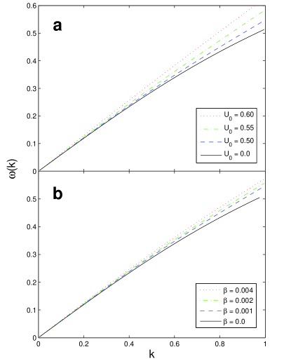
Figure 1: Dispersion curve for harmonic (linear) electron-acoustic waves. Upper panel (a): The variation of the dispersion curve for different values of  $U_{0}$. Curves from bottom to top: $U_{0}=0$  (solid), $0.5$ (dashed), $0.55$ (dot-dashed), and $0.6$ (dotted curve). Bottom panel (b): Variation of the dispersion curve for different values of  $\beta$. Curves from bottom to top: $\beta=0.0$ (solid), $0.001$ (dashed), $0.002$ (dot-dashed curve), and $0.004$ (dotted curve). Here, (a) $\beta=0.001$ (b) $U_{0}=0.5$, and (a-b) $\alpha=1$ and $\kappa=3$.

IV Nonlinear analysis

To obtain solitary wave profile solutions, we consider all fluid variables in a stationary frame traveling at a constant normalized velocity $M$ (to be referred to as the Mach number), implying the transformation $\xi=x-Mt$. This replaces the space and time derivatives with $\partial/\partial x=d/d\xi$ and $\partial/\partial t=-Md/d\xi$, respectively. Now equations (2)-(5) and (7) take the form:

$$-M\dfrac{dn}{d\xi}+\frac{d(nu)}{d\xi}=0,$$ (13)

$$-M\dfrac{du}{d\xi}+u\dfrac{du}{d\xi}=\dfrac{d\phi}{d\xi},$$ (14)

$$-M\dfrac{dn_{b}}{d\xi}+\frac{d(n_{b}u_{b})}{d\xi}=0,$$ (15)

$$-M\dfrac{du_{b}}{d\xi}+u_{b}\dfrac{du_{b}}{d\xi}=\dfrac{d\phi}{d\xi},$$ (16)

$$\dfrac{d^{2}\phi}{d\xi^{2}} =-\left(1+\alpha+\beta\right)+n+\beta n_{b}$$

$$+\alpha\left(1-\frac{\phi}{(\kappa-\tfrac{3}{2})}\right)^{-\kappa+1/2},$$ (17)

The equilibrium state is assumed to be reached at both infinities ($\xi\rightarrow\pm\infty$), so integrating Eqs. (13)–(16) and applying the boundary conditions $n=1$, $u=0$, $n_{b}=1$, $u_{b}=U_{0\text{ }}$ and $\phi=0$ at infinities provide

$$u=M\left[1-\left(\frac{1}{n}\right)\right],$$ (18)

$$u={M-}\left({M}^{2}{+2\phi}\right)^{1/2},$$ (19)

$$u_{b}=M\left[1-\frac{1}{n_{b}}\left(1-\frac{U_{0\text{ }}}{M}\right)\right],$$ (20)

$$u_{b}=M-\left(M^{2}+2\phi-2MU_{0\text{ }}+U_{0}^{2}\right)^{1/2},$$ (21)

Combining Eqs. (18)–(21), one obtains the following equations for the cold electron density and beam electron density, respectively

$$n=\left(1+\dfrac{2\phi}{M^{2}}\right)^{-1/2},$$ (22)

$$n_{b}=\left(1+\dfrac{2\phi}{(M-U_{0\text{ }})^{2}}\right)^{-1/2},$$ (23)

Substituting the density expression (22) and (23) into Poisson’s equation (17) and integrating, yields a pseudo-energy balance equation:

$$\frac{1}{2}\left(\frac{d\phi}{d\xi}\right)^{2}+\Psi(\phi)=0,$$ (24)

where the Sagdeev pseudopotential $\Psi(\phi)$ is given by

$$\Psi(\phi) =\beta(M-U_{0\text{ }})^{2}\left[1-\left(1+\dfrac{2\phi}{(M-U_{0\text{ }})^{2}}\right)^{1/2}\right]$$

$$+\left(1+\alpha+\beta\right)\phi+M^{2}\left[1-\left(1+\dfrac{2\phi}{M^{2}}\right)^{1/2}\right]$$

$$+\alpha\left[1-\left(1-\frac{\phi}{(\kappa-\tfrac{3}{2})}\right)^{-\kappa+3/2}\right].$$ (25)

In the absence of the beam ($\beta\rightarrow 0$), Eq. (25) recovers Eq. (33) given in Ref. [10] in the cold-electron limit ($T_{e}=0$).

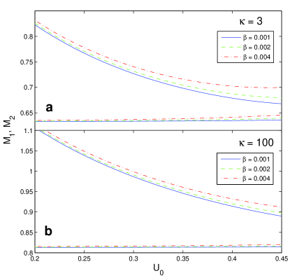
Figure 2: Variation of the lower limit $M_{1}$ (lower curves) and the upper limit $M_{2}$ (upper curves) with the equilibrium beam speed $U_{0}$ for different values of the beam-to-cool electron charge density ratio $\beta$. Curves: $\beta=0.001$ (solid), $0.002$ (dashed), and $0.004$ (dot-dashed). Here, (a) $\kappa=3$, (b) $\kappa=100$ and (a-b) $\alpha=1.5$.

V Soliton existence domain

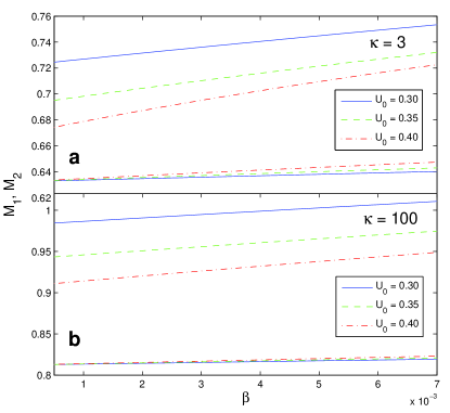
Figure 3: Variation of the lower limit $M_{1}$ (lower curves) and the upper limit $M_{2}$ (upper curves) with the beam-to-cool electron charge density ratio $\beta$ for different values of the equilibrium beam speed $U_{0}$. Curves: $U_{0}=0.3$ (solid), $0.35$ (dashed), and $0.4$ (dot-dashed). Here, we have taken: (a) $\kappa=3$ and (b) $\kappa=100$. Here, we have taken: (a) $\kappa=3$, (b) $\kappa=100$ and (a-b) $\alpha=1.5$.

For existence of solitons, we require that the origin at $\phi=0$ is a root and a local maximum of $\Psi$ in Eq. (25), i.e., $\Psi(\phi)=0$, $d\Psi(\phi)/d\phi=0$ and $d^{2}\Psi(\phi)/d\phi^{2}<0$ at $\phi=0$. The first two constraints are satisfied. We thus impose the condition $F_{1}(M)=-d^{2}\Psi(\phi)/d\phi^{2}|_{\phi=0}>0$, and we get

$$F_{1}(M)=\frac{\alpha(\kappa-\frac{1}{2})}{\kappa-\tfrac{3}{2}}-\frac{1}{M^{2}}-\frac{\beta}{(M-U_{0\text{ }})^{2}}>0$$ (26)

Eq. (26) provides the minimum value for the Mach number $M_{1}$.

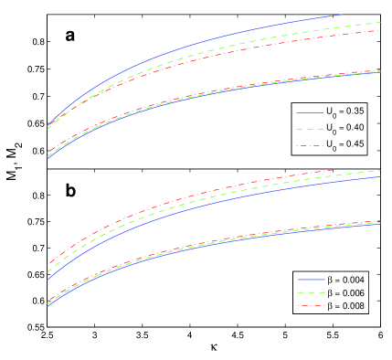
Figure 4: Variation of the lower limit $M_{1}$ (lower curves) and the upper limit $M_{2}$ (upper curves) with the suprathermality parameter $\kappa$ for different values of the equilibrium beam speed $U_{0}$ (a) and the beam-to-cool electron charge density ratio $\beta$ (b). Upper panel (a): $U_{0}=0.35$ (solid curve), $0.40$ (dashed), and $0.45$ (dot-dashed). Middle panel (b): $\beta=0.004$ (solid curve), $0.006$ (dashed), and $0.008$ (dot-dashed). Here, we have taken (a) $\beta=0.004$, (b) $U_{0}=0.4$ and (a-b) $\alpha=1.5$.

An upper limit for M is found through the fact that the cold electron density becomes complex at $\phi_{\lim(-)}=-\frac{1}{2}{M}^{2}$ for $U_{0}\leqslant 0$ and $\phi_{\lim(-)}=-\frac{1}{2}\left(M-U_{0}\right)^{2}$ for $U_{0}>0$, which yield the following equations for the upper limit in $M$ for $U_{0}\leqslant 0$:

$$F_{2}(M) =M^{2}\left(1-\tfrac{1}{2}\left(1+\alpha+\beta\right)\right)$$

$$+\beta(M-U_{0\text{ }})^{2}\left[1-\left(1-\dfrac{M^{2}}{(M-U_{0\text{ }})^{2}}\right)^{1/2}\right]$$

$$+\alpha\left[1-\left(1+\dfrac{M^{2}}{2\kappa-3}\right)^{-\kappa+3/2}\right]$$ (27)

and for $U_{0}>0$:

$$F_{2}(M) =-\tfrac{1}{2}\left(1+\alpha-\beta\right)(M-U_{0})^{2}$$

$$+M^{2}\left[1-\left(1-\dfrac{(M-U_{0})^{2}}{M^{2}}\right)^{1/2}\right]$$

$$+\alpha\left[1-\left(1+\dfrac{(M-U_{0})^{2}}{2\kappa-3}\right)^{-\kappa+3/2}\right]$$ (28)

Solving equations (27) and (28) provides the upper limit $M_{2}$ for acceptable values of the Mach number for solitons to exist. In the absence of the beam ($\beta\rightarrow 0$), Eqs. (26) and (27) yield exactly Eqs. (34) and (36) given in Ref. [10] in the cold-electron limit ($T_{e}=0$).

Figure 2 depicts the existence domain of electron-acoustic solitary waves in two opposite cases: a very low, and a very high value of $\kappa$. We see that the existence domain in Mach number becomes narrower for strong suprathermality and higher values of the equilibrium beam speed $U_{0}$. From two frames (a) and (b) in Fig. 2, it is found that low value of $\kappa$ imposes that the soliton propagates at lower Mach number range. We note that lower values of the beam-to-cold electron charge density ratio ($\beta$; see also Fig. 3) shrink the permitted soliton region for very high $U_{0}$ ($\geqslant 0.5$) and strong suprathermality (low $\kappa$).

As seen in Figs. 2 and 3, the existence region becomes narrower for lower values of $\beta$ and $\kappa$. It is in contrast to increasing the hot-to-cold electron charge density ratio $\alpha$, which shrinks down the existence region [10]. As seen, a high value of the beam speed $U_{0}$ shrinks the permitted region for strong suprathermality (low $\kappa$).

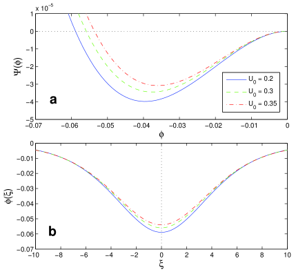
Figure 5: The pseudopotential $\Psi(\phi)$ vs. $\phi$ (a) and the associated electric potential pulse $\phi$ vs. $\xi$ (b) for different values of the equilibrium beam speed $U_{0}$. From bottom to top: $U_{0}=0.2$ (solid curve), $0.3$ (dashed curve), and $0.35$ (dot-dashed curve). Here, we have taken: $\alpha=1$, $\beta=0.008$, $\kappa=4.0$ and $M=0.9$.

Figure 4 shows the effect of a $\kappa$-distribution of hot electrons. The acoustic limits ($M_{1}$ and $M_{2}$) decreases rapidly as approaching the limiting value $\kappa\rightarrow 3/2$. However, going towards a Maxwellian distribution ($\kappa\rightarrow\infty$) broadens the permitted range of the Mach number. The result is similar to the trend in Figs. 2 and 3. It is also similar to what we found in the model without the beam [10].

VI Soliton characteristics

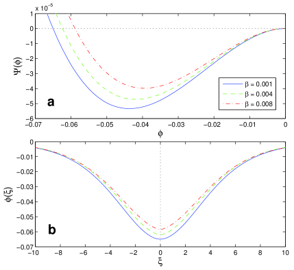
Figure 6: The pseudopotential $\Psi(\phi)$ vs. $\phi$ (a) and the associated electric potential pulse $\phi$ vs. $\xi$ (b) for different values of the beam-to-cool electron charge density ratio $\beta$. From bottom to top: $\beta=0.001$ (solid curve); $0.004$ (dashed curve); $0.008$ (dot-dashed curve). Here, we have taken $\alpha=1$, $U_{0}=0.2$, $\kappa=4.0$ and $M=0.9$.

Figure 5a shows the variation of the pseudopotential $\Psi(\phi)$ with the normalized potential $\phi$, for different values of the beam speed $U_{0}$ (keeping $\alpha=1$, $\beta=0.008$, $\kappa=4$ and $M=0.9$). The electrostatic pulse (soliton) solution shown in Fig. 5b is obtained via numerical integration. As seen, the pulse amplitude $|\phi_{m}|$ decreases with increasing $U_{0}$.

Figure 6 shows the variation of the pseudopotential $\Psi(\phi)$ for different values of the beam-to-cold electron charge density ratio $\beta$. Both the root and the depth of the Sagdeev potential increase with decreasing $\beta=n_{b,0}/n_{c,0}$. This means that either increasing the cold electron density or decreasing the electron beam density increase the negative potential solitary waves.

VII Conclusion

In the present study, we have investigated the linear and nonlinear large-amplitude characteristics of electron-acoustic solitary waves in a plasma consisting of electron beam, hot $\kappa$-distributed electrons, cold background electrons and immobile ions. We derived the linear dispersion relation of our model, and determined the effects of beam parameters on the dispersion characteristics, namely the beam-to-cool electron population ratio $\beta$ and the equilibrium beam speed $U_{0}$. We have used the Sagdeev pseudopotential method to investigate large amplitude localized nonlinear electrostatic structures (solitary waves), and to determine the region in parameter space where stationary profile solutions may exist. We have found only negative potential solitons as apparently the $\kappa$-distribution does not lead to reverse polarity. The existence domain for solitons was found to become narrower with an increase in the suprathermality (decreasing $\kappa$), increasing the beam speed $U_{0}$, decreasing the beam-to-cold electron population ratio $\beta$. We numerically obtained a series of appropriate examples of the electrostatic solitons, which also supports the soliton permitted regions obtained through a root and a local maximum of the pseudopotential. Our results will improve the understanding of solitary waves observed in space electron-beam plasmas, which often include energetic suprathermal electrons.

References

- [1] H. V. Cane, W. C. Erickson, and N. P. Prestage, “Solar flares, type III radio bursts, coronal mass ejections, and energetic particles,” Journal of Geophysical Research (Space Physics), vol. 107, p. 1315, Oct. 2002.
- [2] K.-L. Klein and A. Posner, “The onset of solar energetic particle events: prompt release of deka-MeV protons and associated coronal activity,” Astronomy and Astrophysics, vol. 438, pp. 1029–1042, Aug. 2005.
- [3] M. J. Reiner, K.-L. Klein, M. Karlický, K. Jiřička, A. Klassen, M. L. Kaiser, and J.-L. Bougeret, “Solar Origin of the Radio Attributes of a Complex Type III Burst Observed on 11 April 2001,” Solar Physics, vol. 249, pp. 337–354, Jun. 2008.
- [4] I. H. Cairns and S. F. Fung, “Growth of electron plasma waves above and below f(p) in the electron foreshock,” Journal of Geophysical Research, vol. 93, pp. 7307–7317, Jul. 1988.
- [5] I. H. Cairns, “Fine structure in plasma waves and radiation near the plasma frequency in Earth’s foreshock,” Journal of Geophysical Research, vol. 99, p. 23505, Dec. 1994.
- [6] V. M. Vasyliunas, “A survey of low-energy electrons in the evening sector of the magnetosphere with OGO 1 and OGO 3,” Journal of Geophysical Research, vol. 73, pp. 2839–2884, May 1968.
- [7] D. Summers and R. M. Thorne, “The modified plasma dispersion function,” Physics of Fluids B, vol. 3, pp. 1835–1847, Aug. 1991.
- [8] T. K. Baluku and M. A. Hellberg, “Dust acoustic solitons in plasmas with kappa-distributed electrons and/or ions,” Physics of Plasmas, vol. 15, no. 12, p. 123705, Dec. 2008.
- [9] M. A. Hellberg, R. L. Mace, T. K. Baluku, I. Kourakis, and N. S. Saini, “Comment on “Mathematical and physical aspects of Kappa velocity distribution” [Phys. Plasmas 14, 110702 (2007)],” Physics of Plasmas, vol. 16, no. 9, p. 094701, Sep. 2009.
- [10] A. Danehkar, N. S. Saini, M. A. Hellberg, and I. Kourakis, “Electron-acoustic solitary waves in the presence of a suprathermal electron component,” Physics of Plasmas, vol. 18, no. 7, p. 072902, Jul. 2011.
- [11] ——, “Electron beam–plasma interaction in a dusty plasma with excess suprathermal electrons,” in The 6th International Conference on the Physics of Dusty Plasmas (ICPDP2011), ser. AIP Conference Proceedings, V. Y. Nosenko, P. K. Shukla, M. H. Thoma, and H. M. Thomas, Eds., vol. 1397, Nov. 2011, pp. 305–306.
- [12] N. S. Saini, A. Danehkar, M. A. Hellberg, and I. Kourakis, “Large-amplitude electron-acoustic solitons in a dusty plasma with kappa-distributed electrons,” in The 6th International Conference on the Physics of Dusty Plasmas (ICPDP2011), ser. AIP Conference Proceedings, V. Y. Nosenko, P. K. Shukla, M. H. Thoma, and H. M. Thomas, Eds., vol. 1397, Nov. 2011, pp. 357–358.