Tensor Networks for Dimensionality Reduction and Large-Scale Optimizations
Part 2 Applications and Future Perspectives
A. Cichocki,          A-H. Phan,
Q. Zhao,        N. Lee,
I.V. Oseledets,          M. Sugiyama,
D. Mandic

Abstract

Part 2 of this monograph builds on the introduction to tensor networks and their operations presented in Part 1. It focuses on tensor network models for super-compressed higher-order representation of data/parameters and related cost functions, while providing an outline of their applications in machine learning and data analytics.

A particular emphasis is on the tensor train (TT) and Hierarchical Tucker (HT) decompositions, and their physically meaningful interpretations which reflect the scalability of the tensor network approach. Through a graphical approach, we also elucidate how, by virtue of the underlying low-rank tensor approximations and sophisticated contractions of core tensors, tensor networks have the ability to perform distributed computations on otherwise prohibitively large volumes of data/parameters, thereby alleviating or even eliminating the curse of dimensionality.

The usefulness of this concept is illustrated over a number of applied areas, including generalized regression and classification (support tensor machines, canonical correlation analysis, higher order partial least squares), generalized eigenvalue decomposition, Riemannian optimization, and in the optimization of deep neural networks.

Part 1 and Part 2 of this work can be used either as stand-alone separate texts, or indeed as a conjoint comprehensive review of the exciting field of low-rank tensor networks and tensor decompositions.

Chapter 1 Tensorization and Structured Tensors

The concept of tensorization refers to the generation of higher-order structured tensors from the lower-order data formats (e.g., vectors, matrices or even low-order tensors), or the representation of very large scale system parameters in low-rank tensor formats. This is an essential step prior to multiway data analysis, unless the data itself is already collected in a multiway format; examples include color image sequences where the R, G and B frames are stacked into a 3rd-order tensor, or multichannel EEG signals combined into a tensor with modes, e.g., channel $\times$ time $\times$ epoch. For any given original data format, the tensorization procedure may affect the choice and performance of a tensor decomposition in the next stage.

Entries of the so constructed tensor can be obtained through: $i$) a particular rearrangement, e.g., reshaping of the original data to a tensor, $ii$) alignment of data blocks or epochs, e.g., slices of a third-order tensor are epochs of multi-channel EEG signals, or $iii$) data augmentation through, e.g., Toeplitz and Hankel matrices/tensors. In addition, tensorization of fibers of a lower-order tensor will yield a tensor of higher order. A tensor can also be generated using transform-domain methods, for example, by a time-frequency transformation via the short time Fourier transform or wavelet transform. The latter procedure is most common for multichannel data, such as EEG, where, e.g., $S$ channels of EEG are recorded over $T$ time samples, to produce $S$ matrices of $F\times T$ dimensional time-frequency spectrograms stacked together into an $F\times T\times S$ dimensional third-order tensor. A tensor can also represent the data at multi-scale and orientation levels by using, e.g., the Gabor, countourlet, or pyramid steerable transformations. When exploiting statistical independence of latent variables, tensors can be generated by means of higher-order statistics (cumulants) or by partial derivatives of the Generalised Characteristic Functions (GCF) of the observations. Such tensors are usually partially or fully symmetric, and their entries represent mutual interaction between latent variables. This kind of tensorization is commonly used in ICA, BSS and blind identification of a mixing matrix. In a similar way, a symmetric tensor can be generated through measures of distances between observed entities, or their information exchange. For example, a third-order tensor, created to analyse common structures spread over EEG channels, can comprise distance matrices of pair-wise correlation or other metrics, such as causality over trials. A symmetric third-order tensor can involve three-way similarities. For such a tensorization, symmetric tensor decompositions with nonnegativity constraints are particularly well-suited.

Tensorization can also be performed through a suitable representation of the estimated parameters in some low-rank tensor network formats. This method is often used when the number of estimated parameters is huge, e.g., in modelling system response in a nonlinear system, in learning weights in a deep learning network. In this way, computation on the parameters, e.g., multiplication, convolution, inner product, Fourier transform, can be performed through core tensors of smaller scale.

One of the main motivations to develop various types of tensorization is to take advantage of data super-compression inherent in tensor network formats, especially in quantized tensor train (QTT) formats. In general, the type of tensorization depends on a specific task in hand and the structure presented in data. The next sections introduce some common tensorization methods employed in blind source separation, harmonic retrieval, system identification, multivariate polynomial regression, and nonlinear feature extraction.

1.1 Reshaping or Folding

The simplest way of tensorization is through the reshaping or folding operations, also known as segmentation [Debals and De Lathauwer, 2015, Boussé et al., 2015]. This type of tensorization preserves the number of original data entries and their sequential ordering, as it only rearranges a vector to a matrix or tensor. Hence, folding does not require additional memory space.

Folding. A tensor $\underline{\mathbf{Y}}$ of size $I_{1}\times I_{2}\times\cdots\times I_{N}$ is considered a folding of a vector ${\bf y}$ of length $I_{1}I_{2}\cdots I_{N}$, if

$$\underline{\mathbf{Y}}(i_{1},i_{2},\ldots,i_{N})={\bf y}(i)\,,$$ (1.1)

for all $1\leq i_{n}\leq I_{n}$, where $i=1+\sum_{n=1}^{N}(i_{n}-1)\prod_{k=1}^{n-1}I_{k}$ is a linear index of ($i_{1},i_{2},\ldots,i_{2}$).

In other words, the vector ${\bf y}$ is vectorization of the tensor $\underline{\mathbf{Y}}$, while $\underline{\mathbf{Y}}$ is a tensorization of ${\bf y}$.

As an example, the arrangement of elements in a matrix of size $I\times L/I$, which is folded from a vector ${\bf y}$ of length $L$ is given by

$${\bf Y} = \left[\begin{array}[]{cccc}y(1)&y(I+1)&\cdots&y(L-I+1)\\ y(2)&y(I+2)&\cdots&y(L-I+2)\\ \vdots&\vdots&\ddots&\vdots\\ y(I)&y(2I)&\cdots&y(L)\end{array}\right]\,.$$ (1.6)

Higher-order folding/reshaping refers to the application of the folding procedure several times, whereby a vector ${\bf y}\in\mathbb{R}^{I_{1}I_{2}\cdots I_{N}}$ is converted into an $N$th-order tensor of size $I_{1}\times I_{2}\times\cdots\times I_{N}$.

Application to BSS. It is important to notice that a higher-order folding (quantization) of a vector of length $q^{N}$ $(q=2,3,\ldots)$, sampled from an exponential function $y_{k}=az^{k-1}$, yields an $N$th-order tensor of rank 1. Moreover, wide classes of functions formed by products and/or sums of trigonometric, polynomial and rational functions can be quantized in this way to yield (approximate) low-rank tensor train (TT) network formats [Khoromskij, 2011a, b, Oseledets, 2012]. Exploitation of such low-rank representations allows us to separate the signals from a single or a few mixtures, as outlined below.

Consider a single mixture, $y(t)$, which is composed of $J$ component signals, $x_{j}(t)$, $j=1,\ldots,J$, and corrupted by additive Gaussian noise, $n(t)$, to give

$$y(t)=a_{1}x_{1}(t)+a_{2}x_{2}(t)+\cdots+a_{J}x_{J}(t)+n(t).$$ (1.7)

The aim is to extract the unknown sources (components) $x_{j}(t)$ from the observed signal $y(t)$. Assume that higher-order foldings, $\underline{\mathbf{X}}_{j}$, of the component signals, $x_{j}(t)$, have low-rank representations in, e.g., the CP or Tucker format, given by

$$\underline{\mathbf{X}}_{j}=\llbracket\underline{\mathbf{G}}_{j};{\bf U}_{j}^{(1)},{\bf U}_{j}^{(2)},\ldots,{\bf U}_{j}^{(N)}\rrbracket\,,$$

or in the TT format

$$\underline{\mathbf{X}}_{j}=\mathopen{\hbox{\set@color${\langle}$}\kern-1.94444pt\leavevmode\hbox{\set@color${\langle}$}}\underline{\mathbf{G}}_{j}^{(1)},\underline{\mathbf{G}}_{j}^{(2)},\ldots,\underline{\mathbf{G}}_{j}^{(N)}\mathclose{\hbox{\set@color${\rangle}$}\kern-1.94444pt\leavevmode\hbox{\set@color${\rangle}$}},$$

or in any other tensor network format. Because of the multi-linearity of this tensorization, the following relation between the tensorization of the mixture, $\underline{\mathbf{Y}}$, and the tensorization of the hidden components, $\underline{\mathbf{X}}_{j}$, holds

$$\underline{\mathbf{Y}} = a_{1}\underline{\mathbf{X}}_{1}+a_{2}\underline{\mathbf{X}}_{2}+\cdots+a_{J}\underline{\mathbf{X}}_{J}+\underline{\mathbf{N}}\,,$$ (1.8)

where $\underline{\mathbf{N}}$ is the tensorization of the noise $n(t)$.

Now, by a decomposition of $\underline{\mathbf{Y}}$ into $J$ blocks of tensor networks, each corresponding to a tensor network (TN) representation of a hidden component signal, we can find approximations of $\underline{\mathbf{X}}_{j}$ and the separate component signals up to a scaling ambiguity. The separation method can be used in conjunction with the Toeplitz and Hankel foldings. Example 1.10.1 illustrates the separation of damped sinusoid signals.

1.2 Tensorization through a Toeplitz/Hankel Tensor

1.2.1 Toeplitz Folding

The Toeplitz matrix is a structured matrix with constant entries in each diagonal. Toeplitz matrices appear in many signal processing applications, e.g., through covariance matrices in prediction, estimation, detection, classification, regression, harmonic analysis, speech enhancement, interference cancellation, image restoration, adaptive filtering, blind deconvolution and blind equalization [Bini, 1995, Gray, 2006].

Before introducing a generalization of a Toeplitz matrix to a Toeplitz tensor, we shall first consider the discrete convolution between two vectors ${\bf x}$ and ${\bf y}$ of respective lengths $I$ and $L>I$, given by

$${\bf z}={\bf x}\ast{\bf y}\,.$$ (1.9)

Now, we can write the entries ${\bf z}_{I:L}=\left[z(I),z(I+1),\ldots,z(L)\right]^{\text{T}}$ in a linear algebraic form as

$${\bf z}_{I:L} =\left[\begin{array}[]{cccccc}y(I)&y(I-1)&y(I-2)&\cdots&y(1)\\ y(I+1)&y(I)&y(I-1)&\cdots&y(2)\\ y(I+2)&y(I+1)&y(I)&\cdots&y(3)\\ \vdots&\vdots&\vdots&\ddots&\vdots\\ y(L)&y(L-1)&y(L-2)&\cdots&y(J)\end{array}\right]\,\left[\begin{array}[]{c}x(1)\\ x(2)\\ x(3)\\ \vdots\\ x(I)\end{array}\right]$$ (1.20)

$$={\bf Y}^{\text{T}}{\bf x}={\bf Y}\bar{\times}_{1}{\bf x},$$

where $J=L-I+1$. With this representation, the convolution can be computed through a linear matrix operator, ${\bf Y}$, which is called the Toeplitz matrix of the generating vector ${\bf y}$.

Toeplitz matrix. A Toeplitz matrix of size $I\times J$, which is constructed from a vector ${\bf y}$ of length $L=I+J-1$, is defined as

$${\bf Y}={\mathcal{T}}_{I,J}({\bf y})=\left[\begin{array}[]{cccc}y(I)&y(I+1)&\cdots&y(L)\\ y(I-1)&y(I)&\cdots&y(L-1)\\ \vdots&\vdots&\ddots&\vdots\\ y(1)&y(2)&\cdots&y(L-I+1)\end{array}\right]\,.\;\;$$ (1.25)

The first column and first row of the Toeplitz matrix represent its entire generating vector.

Indeed, all $(L+I-1)$ entries of ${\bf y}$ in the above convolution (1.9) can be expressed either by: (i) using a Toeplitz matrix formed from a zero-padded generating vector $[{\bf 0}_{I-1}^{\text{T}},{\bf y}^{\text{T}},{\bf 0}_{I-1}^{\text{T}}]^{\text{T}}$, with $[{\bf y}^{\text{T}},{\bf 0}_{I-1}^{\text{T}}]$ being the first row of this Toeplitz matrix, to give

$${\bf z}={\mathcal{T}}_{I,L+I-1}([{\bf 0}_{I-1}^{\text{T}},{\bf y}^{\text{T}},{\bf 0}_{I-1}^{\text{T}}]^{\text{T}})^{\text{T}}\,{\bf x}\,,$$ (1.26)

or (ii) through a Toeplitz matrix of the generating vector $[{\bf 0}_{L-1}^{\text{T}},{\bf x}^{\text{T}},{\bf 0}_{L-1}^{\text{T}}]^{\text{T}}$, to yield

$${\bf z}={\mathcal{T}}_{L,L+I-1}([{\bf 0}_{L-1}^{\text{T}},{\bf x}^{\text{T}},{\bf 0}_{L-1}^{\text{T}}]^{\text{T}})^{\text{T}}\,{\bf y}\,.$$ (1.27)

The so expanded Toeplitz matrix is a circulant matrix of $[{\bf y}^{\text{T}},{\bf 0}_{I-1}^{\text{T}}]^{\text{T}}$.

Consider now a convolution of three vectors, ${\bf x}_{1}$, ${\bf x}_{2}$ and ${\bf y}$ of respective lengths $I_{1}$, $I_{2}$ and $(L\geq I_{1}+I_{2})$, given by

$${\bf z}={\bf x}_{1}\ast{\bf x}_{2}\ast{\bf y}\,.$$

For its implementation, we first construct a Toeplitz matrix, ${\bf Y}$, of size $I_{1}\times(L-I_{1}+1)$ from the generating vector ${\bf y}$. Then, we use the rows ${\bf Y}(k,:)$ to generate Toeplitz matrices, ${\bf Y}_{k}$ of size $I_{2}\times I_{3}$. Finally, all $I_{1}$ Toeplitz matrices, ${\bf Y}_{1}$, …, ${\bf Y}_{I_{1}}$, are stacked as horizontal slices of a third-order tensor $\underline{\mathbf{Y}}$, i.e., $\underline{\mathbf{Y}}(k,:,:)={\bf Y}_{k}$, $k=1,\ldots,I_{1}$. It can be verified that entries $[z(I_{1}+I_{2}-1),\ldots,z(L)]^{T}$ can be computed as

$$\left[\begin{array}[]{cccc}z(I_{1}+I_{2}-1)\\ \vdots\\ z(L)\end{array}\right]=[{\bf x}_{1}\ast{\bf x}_{2}\ast{\bf y}]_{I_{1}+I_{2}-1:L} = \underline{\mathbf{Y}}\,\bar{\times}_{1}\,{\bf x}_{1}\,\bar{\times}_{2}\,{\bf x}_{2}.$$ (1.31)

The tensor $\underline{\mathbf{Y}}$ is referred to as the Toeplitz tensor of the generating vector ${\bf y}$.

Toeplitz tensor. An $N$th-order Toeplitz tensor of size $I_{1}\times I_{2}\times\cdots\times I_{N}$, which is represented by $\underline{\mathbf{Y}}={\mathcal{T}}_{I_{1},\ldots,I_{N}}({\bf y})$, is constructed from a generating vector ${\bf y}$ of length $L=I_{1}+I_{2}+\cdots+I_{N}-N+1$, such that its entries are defined as

$$\underline{\mathbf{Y}}(i_{1},\ldots,i_{N-1},i_{N})=y(\bar{i}_{1}+\cdots+\bar{i}_{N-1}+i_{N})\,,$$ (1.32)

where $\bar{i}_{n}=I_{n}-i_{n}$. An example of the Toeplitz tensor is illustrated in Figure 1.1.

Example 1  Given a $3\times 3\times 3$ dimensional Toeplitz tensor of a sequence $1,2,\ldots,7$, the horizontal slices are Toeplitz matrices of sizes $3\times 3$ given by

$${\mathcal{T}}_{3,3,3}(1,\ldots,7) =\left[\begin{array}[]{cccc}{\mathcal{T}}_{3,3}(3,\ldots,7)\\ {\mathcal{T}}_{3,3}(2,\ldots,6)\\ {\mathcal{T}}_{3,3}(1,\ldots,5)\end{array}\right]=\left[\begin{array}[]{c}\left[\begin{array}[]{cccc}5&6&7\\ 4&5&6\\ 3&4&5\end{array}\right]\\ \left[\begin{array}[]{cccc}4&5&6\\ 3&4&5\\ 2&3&4\\ \end{array}\right]\\ \left[\begin{array}[]{cccc}3&4&5\\ 2&3&4\\ 1&2&3\\ \end{array}\right]\end{array}\right]\,.$$ (1.48)

Figure 1.1: Illustration of a 3rd-order Toeplitz tensor of size $I_{1}\times I_{2}\times I_{3}$, generated from a vector ${\bf y}$ of length $L=I_{1}+I_{2}+I_{3}-2$. (a) The highlighted fibers of the Toeplitz tensor form the generating vector ${\bf y}$. (b) The entries in every shaded diagonal intersection are identical and represent one element of ${\bf y}$.

Recursive generation. An $N$th-order Toeplitz tensor of a generating vector ${\bf y}$ is of size $I_{1}\times I_{2}\times\cdots\times I_{N}$, can be constructed from an $(N-1)$th-order Toeplitz tensor of size $I_{1}\times I_{2}\times\cdots\times(I_{N-1}+I_{N}-1)$ of the same generating vector, by a conversion of mode-$(N-1)$ fibers to Toeplitz matrices of size $I_{N-1}\times I_{N}$.

Following the definition of the Toeplitz tensor, the convolution of $(N-1)$ vectors, ${\bf x}_{n}$ of respective lengths $I_{n}$, and a vector ${\bf y}$ of length $L$, can be represented as a tensor-vector product of an $N$th-order Toeplitz tensor and vectors ${\bf x}_{n}$, that is

$$[{\bf x}_{1}\ast{\bf x}_{2}\ast\cdots\ast{\bf x}_{N-1}\ast{\bf y}]_{J:L}=\underline{\mathbf{Y}}\,\bar{\times}_{1}\,{\bf x}_{1}\,\bar{\times}_{2}\,{\bf x}_{2}\cdots\bar{\times}_{N-1}\,{\bf x}_{N-1}\,,$$

where $\underline{\mathbf{Y}}={\mathcal{T}}_{I_{1},\ldots,I_{N-1},L-J}({\bf y})$ is a Toeplitz tensor of size $I_{1}\times\cdots\times I_{N-1}\times(L-J)$ generated from ${\bf y}$, and $J=\sum_{n=1}^{N-1}I_{n}-N+1$, or

$${\bf x}_{1}\ast{\bf x}_{2}\ast\cdots\ast{\bf x}_{N-1}\ast{\bf y}=\widetilde{\underline{\mathbf{Y}}}\,\bar{\times}_{1}\,{\bf x}_{1}\,\bar{\times}_{2}\,{\bf x}_{2}\cdots\bar{\times}_{N-1}\,{\bf x}_{N-1}\,,$$

where $\widetilde{\underline{\mathbf{Y}}}={\mathcal{T}}_{I_{1},\ldots,I_{N-1},L+J}([{\bf 0}_{J}^{\text{T}},{\bf y}^{\text{T}},{\bf 0}_{J}^{\text{T}}]^{\text{T}})$ is a Toeplitz tensor, of the zero-padded vector of ${\bf y}$, is of size $I_{1}\times\cdots\times I_{N-1}\times(L+J)$.

1.2.2 Hankel Folding

The Hankel matrix and Hankel tensor have similar structures to the Toeplitz matrix and tensor and can also be used as linear operators in the convolution.

Hankel matrix. An $I\times J$ Hankel matrix of a vector ${\bf y}$, of length $L=I+J-1$, is defined as

$${\bf Y}={\mathcal{H}}_{I,J}({\bf y}) = \left[\begin{array}[]{cccc}y(1)&y(2)&\cdots&y(J)\\ y(2)&y(3)&\cdots&y(J+1)\\ \vdots&\vdots&\ddots&\vdots\\ y(I)&y(I+1)&\cdots&y(L)\end{array}\right]\,.$$ (1.53)

Hankel tensor. [Papy et al., 2005] An $N$th-order Hankel tensor of size $I_{1}\times I_{2}\times\cdots\times I_{N}$, which is represented by $\underline{\mathbf{Y}}={\mathcal{H}}_{I_{1},\ldots,I_{N}}({\bf y})$, is constructed from a generating vector ${\bf y}$ of length $L=\sum_{n}I_{n}-N+1$, such that its entries are defined as

$$\underline{\mathbf{Y}}(i_{1},i_{2},\ldots,i_{N})=y(i_{1}+i_{2}+\cdots+i_{N}-N+1)\,.$$ (1.54)

Remark 1

(Properties of a Hankel tensor)

• The generating vector ${\bf y}$ can be reconstructed by a concatenation of fibers of the Hankel tensor $\underline{\mathbf{Y}}(I_{1},\ldots,I_{n-1},:,1,\ldots,1)$, where $n=1,\ldots,N-1$, and

  $${\bf y}=\left[\begin{array}[]{c}\underline{\mathbf{Y}}(1:I_{1}-1,1,\ldots,1)\\ \vdots\\ \underline{\mathbf{Y}}(I_{1},\ldots,I_{n-1},1:I_{n}-1,1,\ldots,1)\\ \vdots\\ \underline{\mathbf{Y}}(I_{1},\ldots,I_{N-1},1:I_{N})\\ \end{array}\right]\,.$$ (1.60)

• Slices of a Hankel tensor $\underline{\mathbf{Y}}$, i.e., any subset of the tensor produced by fixing $(N-2)$ indices of its entries and varying the two remaining indices, are also Hankel matrices.

• An $N$th-order Hankel tensor, ${\mathcal{H}}_{I_{1},\ldots,I_{N-1},I_{N}}({\bf y})$, can be constructed from an $(N-1)$th-order Hankel tensor ${\mathcal{H}}_{I_{1},\ldots,I_{N-2},I_{N-1}+I_{N}-1}({\bf y})$ of size $I_{1}\times\cdots\times I_{N-2}\times(I_{N-1}+I_{N}-1)$ by converting its mode-$(N-1)$ fibers to Hankel matrices of size $I_{N-1}\times I_{N}$.

• Similarly to the Toeplitz tensor, the convolution of $(N-1)$ vectors, ${\bf x}_{n}$ of lengths $I_{n}$, and a vector ${\bf y}$ of length $L$, can be represented as

  $$[{\bf x}_{1}\ast{\bf x}_{2}\ast\cdots\ast{\bf x}_{N-1}\ast{\bf y}]_{J:L}=\underline{\mathbf{Y}}\,\bar{\times}_{1}\,\tilde{{\bf x}}_{1}\,\bar{\times}_{2}\,\tilde{{\bf x}}_{2}\cdots\bar{\times}_{N-1}\,\tilde{{\bf x}}_{N-1},$$

  or

  $${\bf x}_{1}\ast{\bf x}_{2}\ast\cdots\ast{\bf x}_{N-1}\ast{\bf y}=\widetilde{\underline{\mathbf{Y}}}\,\bar{\times}_{1}\,\tilde{{\bf x}}_{1}\,\bar{\times}_{2}\,\tilde{{\bf x}}_{2}\cdots\bar{\times}_{N-1}\,\tilde{{\bf x}}_{N-1},$$

  where $\tilde{{\bf x}}_{n}=[x_{n}(I_{n}),\ldots,x_{n}(2),x_{n}(1)]$, $J=\sum_{n}I_{n}-N+1$, $\underline{\mathbf{Y}}={\mathcal{H}}_{I_{1},\ldots,I_{N-1},L-J}({\bf y})$ is the $N$th-order Hankel tensor of ${\bf y}$, whereas $\widetilde{\underline{\mathbf{Y}}}={\mathcal{H}}_{I_{1},\ldots,I_{N-1},L+J}([{\bf 0}_{J}^{\text{T}},{\bf y}^{\text{T}},{\bf 0}_{J}^{\text{T}}]^{\text{T}})$ is the Hankel tensor of a zero-padded version of ${\bf y}$.

• A Hankel tensor with identical dimensions $I_{n}=I$, for all $n$, is a symmetric tensor.

Example 2  A $3\times 3\times 3$ – dimensional Hankel tensor of a sequence $1,2,\ldots,7$ is a symmetric tensor, and is given by

$${\mathcal{H}}_{3,3,3}(1:7) = \left[\left[\begin{array}[]{cccc}1&2&3\\ 2&3&4\\ 3&4&5\end{array}\right],\left[\begin{array}[]{cccc}2&3&4\\ 3&4&5\\ 4&5&6\end{array}\right],\left[\begin{array}[]{cccc}3&4&5\\ 4&5&6\\ 5&6&7\end{array}\right]\right]\,.$$ (1.70)

1.2.3 Quantized Tensorization

It is important to notice that the tensorizations into the Toeplitz and Hankel tensors typically enlarge the number of data samples (in the sense that the number of entries of the corresponding tensor is larger than the number of original samples). For example, when the dimensions $I_{n}=2$ for all $n$, the so generated tensor to be a quantized tensor of order $(L-1)$, while the number of entries of a such tensor increases from the original size $L$ to $2^{L-1}$. Therefore, quantized tensorizations are suited to analyse signals of short-length, especially in multivariate autoregressive modelling.

1.2.4 Convolution Tensor

Consider again the convolution ${\bf x}\ast{\bf y}$ of two vectors of respective lengths $I$ and $L$. We can then rewrite the expression for the entries-$(I,I+1,\ldots,L)$ as

$$[{\bf x}\ast{\bf y}]_{I:L}=\underline{\mathbf{C}}\,{\bar{\times}}_{1}\,{\bf x}\,{\bar{\times}}_{3}\,{\bf y}\,,$$

where $\underline{\mathbf{C}}$ is a third-order tensor of size $I\times J\times L$, $J=L-I+1$, for which the $(l-I)$-th diagonal elements of $l$-th slices are ones, and the remaining entries are zeros, for $l=1,2,\ldots,L$. For example, the slices $\underline{\mathbf{C}}(:,:,l)$, for $l\leq I$, are given by

$$\underline{\mathbf{C}}(:,:,l)=\blockarray{cccccc}\block{c[ccccc]}&00\\ \\ 1\ddots\\ \ddots\\ 010\\ &{l}\,.$$

The tensor $\underline{\mathbf{C}}$ is called the convolution tensor. Illustration of a convolution tensor of size $I\times I\times(2I-1)$ is given in Figure 1.2.

Figure 1.2: Visualization of a convolution tensor of size $I\times I\times(2I-1)$. Unit entries are located on the shaded parallelogram.

Note that a product of this tensor with the vector ${\bf y}$ yields the Toeplitz matrix of the generating vector ${\bf y}$, which is of size $I\times J$, in the form

$$\underline{\mathbf{C}}\,\bar{\times}_{3}\,{\bf y}={\mathcal{T}}_{I,J}({\bf y})\,,$$

while the tensor-vector product $\underline{\mathbf{C}}\bar{\times}_{1}{\bf x}$ yields a Toeplitz matrix of the generating vector $[{\bf 0}_{L-I}^{\text{T}},{\bf x}^{\text{T}},{\bf 0}_{J-1}^{\text{T}}]^{\text{T}}$, or a circulant matrix of $[{\bf 0}_{L-I}^{\text{T}},{\bf x}^{\text{T}}]^{\text{T}}$

$$\underline{\mathbf{C}}\,\bar{\times}_{1}\,{\bf x}={\mathcal{T}}_{L,J}([{\bf 0}_{L-I}^{\text{T}},{\bf x}^{\text{T}},{\bf 0}_{J-1}^{\text{T}}]^{\text{T}})\,.$$

In general, for a convolution of $(N-1)$ vectors, ${\bf x}_{1}$, …, ${\bf x}_{N-1}$, of respective lengths $I_{1},\ldots,I_{N-1}$ and a vector ${\bf y}$ of length $L$

$${\bf z}={\bf x}_{1}\ast{\bf x}_{2}\ast\cdots\ast{\bf x}_{N-1}\ast{\bf y}\,,$$ (1.71)

the entries of ${\bf z}$ can be expressed through a multilinear product of a convolution tensor, $\underline{\mathbf{C}}$, of $(N+1)$th-order and size $I_{1}\times I_{2}\times\cdots\times I_{N}\times L$, $I_{N}=L-\sum_{n=1}^{N-1}I_{n}+N-1$, and the $N$ input vectors

$${\bf z}_{L-I_{N}+1:L}=\underline{\mathbf{C}}\,{\bar{\times}}_{1}\,{\bf x}_{1}\,{\bar{\times}}_{2}\,{\bf x}_{2}\cdots\,{\bar{\times}}_{N-1}\,{\bf x}_{N-1}\,{\bar{\times}}_{N+1}\,{\bf y}\,.$$ (1.72)

Most entries of $\underline{\mathbf{C}}$ are zeros, except for those located at $(i_{1},i_{2},\ldots,i_{N+1})$, such that

$$\sum_{n=1}^{N-1}\bar{i}_{n}+i_{N}-i_{N+1}=0\,,$$ (1.73)

where $\bar{i}_{n}=I_{n}-i_{n}$, $i_{n}=1,2,\ldots,I_{n}$.

The tensor product $\underline{\mathbf{C}}{\bar{\times}}_{N+1}\,{\bf y}$ yields the Toeplitz tensor of the generating vector ${\bf y}$, shown below

$$\underline{\mathbf{C}}\,{\bar{\times}}_{N+1}\,{\bf y}={\mathcal{T}}_{I_{1},\ldots,I_{N}}({\bf y}).$$ (1.74)

1.2.5 QTT Representation of the Convolution Tensor

An important property of the convolution tensor is that it has a QTT representation with rank no larger than the number of inputs vectors, $N$. To illustrate this property, for simplicity, we consider an $N$th-order Toeplitz tensor of size $I\times I\times\cdots\times I$ generated from a vector of length $(N\,I-N+1)$, where $I=2^{D}$. The convolution tensor of this Toeplitz tensor is of $(N+1)$th-order and of size $I\times I\times\cdots\times I\times(N\,I-N+1)$.

Zero-padded convolution tensor. By appending $(N-1)$ zero tensors of size $I\times I\times\cdots\times I$ before the convolution tensor, we obtain an $(N+1)$th-order convolution tensor, $\underline{\mathbf{C}},$ of size $I\times I\times\cdots\times I\times IN$.

QTT representation. The zero-padded convolution tensor can be represented in the following QTT format

$$\underline{\mathbf{C}}=\widetilde{\underline{\mathbf{C}}}^{(1)}\,\,|\!\!\otimes\!\!|\,\,\widetilde{\underline{\mathbf{C}}}^{(2)}\,\,|\!\!\otimes\!\!|\,\cdots\,|\!\!\otimes\!\!|\,\,\widetilde{\underline{\mathbf{C}}}^{(D)}\,\,|\!\!\otimes\!\!|\,\,\widetilde{\underline{\mathbf{C}}}^{(D+1)}\,,$$ (1.75)

where “$\,|\!\!\otimes\!\!|\,$” represents the strong Kronecker product between block tensors $\widetilde{\underline{\mathbf{C}}}^{(n)}=[\widetilde{\underline{\mathbf{C}}}^{(n)}_{r,s}]$ defined from the $(N+3)$th-order core tensors $\underline{\mathbf{C}}^{(n)}$ as $\widetilde{\underline{\mathbf{C}}}^{(n)}_{r,s}=\underline{\mathbf{C}}^{(n)}(r,:,\ldots,:,s)$.

The last core tensor $\underline{\mathbf{C}}^{(D+1)}$ represents an exchange (backward identity) matrix of size $N\times N$ which can represented as an $(N+3)$th-order tensor of size $N\times 1\times\cdots\times 1\times N\times 1$. The first $D$ core tensors $\underline{\mathbf{C}}^{(1)}$, $\underline{\mathbf{C}}^{(2)}$, …, $\underline{\mathbf{C}}^{(D)}$ are expressed based on the so-called elementary core tensor $\underline{\mathbf{S}}$ of size $N\times\underbrace{2\times 2\times\cdots\times 2}_{\text{$(N+1)$ dimensions}}\times N$, as

$$\underline{\mathbf{C}}^{(1)}=\underline{\mathbf{S}}(1,:,\ldots,:),\quad\underline{\mathbf{C}}^{(2)}=\cdots=\underline{\mathbf{C}}^{(D)}=\underline{\mathbf{S}}\,.$$ (1.76)

The rigorous definition of the elementary core tensor is provided in Appendix 3.

Table 1.1 provides ranks of the QTT representation for various order of convolution tensors. The elementary core tensor $\underline{\mathbf{S}}$ can be further re-expressed in a (tensor train) TT-format with $(N+1)$ sparse TT cores, as

$$\underline{\mathbf{S}}=\mathopen{\hbox{\set@color${\langle}$}\kern-1.94444pt\leavevmode\hbox{\set@color${\langle}$}}\underline{\mathbf{G}}^{(1)},\underline{\mathbf{G}}^{(2)},\ldots,\underline{\mathbf{G}}^{(N+1)}\mathclose{\hbox{\set@color${\rangle}$}\kern-1.94444pt\leavevmode\hbox{\set@color${\rangle}$}}\,,$$

where $\underline{\mathbf{G}}^{(k)}$ is of size $(N+k-1)\times 2\times(N+k)$, for $k=1,\ldots,N$, and the last core tensor $\underline{\mathbf{G}}^{(N+1)}$ is of size $2N\times 2\times N$.

Table 1.1: Rank of QTT representations of convolution tensors of $(N+1)$th-order for $N=2,\ldots,17$.

$N$ QTT rank $N$ QTT rank 2 2, 2, 2, …, 2 10 6, 8, 9, …, 9 3 2, 3, 3, …, 3 11 6, 9, 10, …, 10 4 3, 4, 4, …, 4 12 7, 10, 11, …, 11 5 3, 4, 5, …, 5 13 7, 10, 12, …, 12 6 4, 5, 6, …, 6 14 8, 11, 13, …, 13 7 4, 6, 7, …, 7 15 8, 12, 14, …, 14 8 5, 7, 8, …, 8 16 9, 13, 15, …, 15 9 5, 7, 8, …, 8 17 9, 13, 15, …, 15

Example 3  Convolution tensor of 3rd-order.

For the vectors ${\bf x}$ of length $2^{D}$ and ${\bf y}$ of length $(2^{D+1}-1)$, the expanded convolution tensor has size of $2^{D}\times 2^{D}\times 2^{D+1}$. The elementary core tensor $\underline{\mathbf{S}}$ is then of size $2\times 2\times 2\times 2\times 2$ and its sub-tensors, $\underline{\mathbf{S}}(i,:,:,:,:)$, are given in a $2\times 2$ block form of the last two indices through four matrices, ${\bf S}_{1}$, ${\bf S}_{2}$, ${\bf S}_{3}$ and ${\bf S}_{4}$, of size $2\times 2$, that is

$$\underline{\mathbf{S}}(1,:,:,:,:) =\left[\begin{array}[]{cc}{\bf S}_{1}&{\bf S}_{3}\\ {\bf S}_{2}&{\bf S}_{4}\end{array}\right]\,,\quad\underline{\mathbf{S}}(2,:,:,:,:)=\left[\begin{array}[]{cc}{\bf S}_{2}&{\bf S}_{4}\\ {\bf S}_{3}&{\bf S}_{1}\end{array}\right]\,,$$ (1.81)

where

$${\bf S}_{1}=\left[\begin{array}[]{cc}1&0\\ 0&1\end{array}\right],\,{\bf S}_{2}=\left[\begin{array}[]{cc}0&1\\ 0&0\end{array}\right],\,{\bf S}_{3}=\left[\begin{array}[]{cc}0&0\\ 0&0\end{array}\right],\,{\bf S}_{4}=\left[\begin{array}[]{cc}0&0\\ 1&0\end{array}\right].\,\,$$ (1.90)

The convolution tensor can then be represented in a QTT format of rank-2 [Kazeev et al., 2013] with core tensors $\underline{\mathbf{C}}^{(2)}=\cdots=\underline{\mathbf{C}}^{(D)}=\underline{\mathbf{S}}$, $\underline{\mathbf{C}}^{(1)}=\underline{\mathbf{S}}(1,:,:,:,:)$, and the last core tensor $\underline{\mathbf{C}}^{(D+1)}=\left[\begin{array}[]{cc}0&1\\ 1&0\end{array}\right]$ which is of size $2\times 1\times 1\times 2\times 1$. This QTT representation is useful to generate a Toeplitz matrix when its generating vector is given in the QTT format. An illustration of the convolution tensor $\underline{\mathbf{C}}$ is provided in Figure 1.3.

Figure 1.3: Representation of the convolution tensor in QTT format. (Top) Distributed representation of a convolution tensor $\underline{\mathbf{C}}$ of size $I\times J\times 2I$ in a QTT format, where $I=J=2^{D}$. The first core tensor $\underline{\mathbf{C}}^{(1)}$ is of size $1\times 2\times 2\times 2\times 2$, the last core tensor $\underline{\mathbf{C}}^{(D+1)}$ represents a backward identity matrix, and the remaining 5th-order core tensors of size $2\times 2\times 2\times 2\times 2$ are identical. A vector ${\bf y}$ is of length $2^{D+1}$ in a QTT format. (Bottom) Generation of the Toeplitz matrix, ${\mathcal{T}}({\bf y})$, of the vector ${\bf y}$ from the convolution tensor and its representation in the QTT format, $I_{d}=J_{d}=2$ for $d=1,\ldots,D$.

Example 4  Convolution tensor of fourth-order.

For the convolution tensor of fourth order, i.e., Toeplitz order $N=3$, the elementary core tensor $\underline{\mathbf{S}}$ is of size $3\times 2\times 2\times 2\times 2\times 3$, and is given in a $2\times 3$ block form of the last two indices as

$$\underline{\mathbf{S}}(1,:,\ldots,:) =\left[\begin{array}[]{ccc}\underline{\mathbf{S}}_{1}&\underline{\mathbf{S}}_{3}&\underline{\mathbf{S}}_{5}\\ \underline{\mathbf{S}}_{2}&\underline{\mathbf{S}}_{4}&\underline{\mathbf{S}}_{6}\end{array}\right]\,,\quad\underline{\mathbf{S}}(2,:,\ldots,:)=\left[\begin{array}[]{ccc}\underline{\mathbf{S}}_{2}&\underline{\mathbf{S}}_{4}&\underline{\mathbf{S}}_{6}\\ \underline{\mathbf{S}}_{5}&\underline{\mathbf{S}}_{1}&\underline{\mathbf{S}}_{3}\end{array}\right]\,,$$ (1.95)

$$\underline{\mathbf{S}}(3,:,\ldots,:) =\left[\begin{array}[]{ccc}\underline{\mathbf{S}}_{5}&\underline{\mathbf{S}}_{1}&\underline{\mathbf{S}}_{3}\\ \underline{\mathbf{S}}_{6}&\underline{\mathbf{S}}_{2}&\underline{\mathbf{S}}_{4}\end{array}\right]\,.$$ (1.98)

where $\underline{\mathbf{S}}_{n}$ are of size $2\times 2\times 2$, $\underline{\mathbf{S}}_{5}$, $\underline{\mathbf{S}}_{6}$ are zero tensors, and

$$\underline{\mathbf{S}}_{1} =\left[\left[\begin{array}[]{cc}1&0\\ 0&0\end{array}\right]\left[\begin{array}[]{cc}0&1\\ 1&0\end{array}\right]\right]\;,\quad\underline{\mathbf{S}}_{2}=\left[\left[\begin{array}[]{cc}0&0\\ 0&0\end{array}\right]\left[\begin{array}[]{cc}1&0\\ 0&0\end{array}\right]\right]\;,$$ (1.107)

$$\underline{\mathbf{S}}_{3} =\left[\left[\begin{array}[]{cc}0&0\\ 0&1\end{array}\right]\left[\begin{array}[]{cc}0&0\\ 0&0\end{array}\right]\right]\;,\quad\underline{\mathbf{S}}_{4}=\left[\left[\begin{array}[]{cc}0&1\\ 1&0\end{array}\right]\left[\begin{array}[]{cc}0&0\\ 0&1\end{array}\right]\right]\;.$$ (1.116)

Finally, the zero-padded convolution tensor of size $2^{D}\times 2^{D}\times 2^{D}\times 3\cdot 2^{D}$ has a QTT representation in (1.75) with $\underline{\mathbf{C}}^{(1)}=\underline{\mathbf{S}}(1,:,:,:,:,[1,2])$, $\underline{\mathbf{C}}^{(2)}=\underline{\mathbf{S}}([1,2],:,:,:,:,:)$, $\underline{\mathbf{C}}^{(3)}=\cdots=\underline{\mathbf{C}}^{(D)}=\underline{\mathbf{S}}$, and the last core tensor $\underline{\mathbf{C}}_{D+1}=\left[\begin{array}[]{ccc}0&0&1\\ 0&1&0\\ 1&0&0\end{array}\right]$ which is of size $3\times 1\times 1\times 3\times 1$.

1.2.6 Low-rank Representation of Hankel and Toeplitz Matrices/Tensors

The Hankel and Toeplitz foldings are multilinear tensorizations, and can be applied to the BSS problem, as in (1.8). When the Hankel and Toeplitz tensors of the hidden sources are of low-rank in some tensor network representation, the tensor of the mixture is expressed as a sum of low rank tensor terms.

For example, the Hankel and Toeplitz matrices/tensors of an exponential function, $v_{k}=az^{k-1}$, are rank-1 matrices/tensors, and consequently Hankel matrices/tensors of sums and/or products of exponentials, sinusoids, and polynomials will also be of low-rank, which is equal to the degree of the function being considered.

Hadamard Product. More importantly, when Hankel/Toeplitz tensors of two vectors ${\bf u}$ and ${\bf v}$ have low-rank CP/TT representations, the Hankel/Toeplitz tensor of their element-wise product, ${\bf w}={\bf u}\circledast{\bf v}$, can also be represented in the same CP/TT tensor format

$${\mathcal{H}}({\bf u})\circledast{\mathcal{H}}({\bf v}) = {\mathcal{H}}({\bf u}\circledast{\bf v})$$

$${\mathcal{T}}({\bf u})\circledast{\mathcal{T}}({\bf v}) = {\mathcal{T}}({\bf u}\circledast{\bf v})\,.$$

The CP/TT rank of ${\mathcal{H}}({\bf u}\circledast{\bf v})$ or ${\mathcal{T}}({\bf u}\circledast{\bf v})$ is not larger than the product of the CP/TT ranks of the tensors of ${\bf u}$ and ${\bf v}$.

Example 5 

The third-order Hankel tensor of $u(t)=\sin(\omega t)$ is a rank-3 tensor, and the third-order Hankel tensor of $v(t)=t$ is of rank-2; hence the Hankel tensor of the $w(t)=t\,\sin(\omega t)$ has at most rank-6.

Symmetric CP and Vandermonde decompositions. It is important to notice that a Hankel tensor $\underline{\mathbf{Y}}$ of size $I\times I\times\cdots\times I$ can always be represented by a symmetric CP decomposition

$$\underline{\mathbf{Y}}=\underline{\mathbf{I}}\times_{1}{\bf A}\times_{2}{\bf A}\cdots\times_{N}{\bf A}\,.$$

Moreover, the tensor $\underline{\mathbf{Y}}$ also admits a symmetric CP decomposition with Vandermonde structured factor matrix [Qi, 2015]

$$\underline{\mathbf{Y}}=\mathop{\rm diag}\nolimits_{N}(\mbox{\boldmath$\lambda$})\times_{1}{\bf V}^{\text{T}}\times_{2}{\bf V}^{\text{T}}\cdots\times_{N}{\bf V}^{\text{T}}\,,$$ (1.117)

where $\lambda$ comprises $R$ non-zero coefficients, and ${\bf V}$ is a Vandermonde matrix generated from $R$ distinct values ${\bf v}=[v_{1},v_{2},\ldots,v_{R}]$

$${\bf V}=\left[\begin{array}[]{ccccc}1&v_{1}&v_{1}^{2}&\ldots&v_{1}^{I-1}\\ 1&v_{2}&v_{2}^{2}&\ldots&v_{2}^{I-1}\\ \vdots&\vdots&\vdots&\ddots&\vdots\\ 1&v_{R}&v_{R}^{2}&\ldots&v_{R}^{I-1}\end{array}\right]\,.$$ (1.122)

By writing the decomposition in (1.117) for the entries $\underline{\mathbf{Y}}(I_{1},\ldots,I_{n-1},:,1,\ldots,1)$ (see (1.60)), the Vandermonde decomposition of the Hankel tensor $\underline{\mathbf{Y}}$ becomes a Vandermonde factorization of ${\bf y}$ [Chen, 2016], given by

$${\bf y}=\left[\begin{array}[]{ccccc}1&1&\ldots&1\\ v_{1}&v_{2}&\ldots&v_{R}\\ v_{1}^{2}&v_{2}^{2}&\ldots&v_{R}^{2}\\ \vdots&\vdots&\ddots&\vdots\\ v_{1}^{L-1}&v_{2}^{L-1}&\ldots&v_{R}^{L-1}\\ \end{array}\right]\mbox{\boldmath$\lambda$}\,.$$ (1.128)

Observe that various Vandermonde decompositions of the Hankel tensors of the same vector ${\bf y}$, but of different tensor orders $N$, have the same generating Vandermonde vector ${\bf v}$. Moreover, the Vandemonde rank, i.e, the minimum of $R$ in the decomposition (1.117), therefore cannot exceed the length $L$ of the generating vector ${\bf y}$.

QTT representation of Toeplitz/Hankel tensor. As mentioned previously, the zero-padded convolution tensor of $(N+1)$th-order can be represented in a QTT format of rank of at most $N$. Hence, if a vector ${\bf y}$ of length $2^{D}N$ has a QTT representation of rank-$(R_{1},\ldots,R_{D})$, given by

$${\bf y}=\widetilde{{\bf Y}}^{(1)}\,|\!\!\otimes\!\!|\,\widetilde{{\bf Y}}^{(2)}\,|\!\!\otimes\!\!|\,\cdots\,|\!\!\otimes\!\!|\,\widetilde{{\bf Y}}^{(D+1)}\,,$$ (1.129)

where $\widetilde{{\bf Y}}^{(d)}$ is an $R_{d-1}\times R_{d}$ block matrix of the core tensor $\underline{\mathbf{Y}}^{(d)}$ of size $R_{d-1}\times 2\times R_{d}$, for $d=1,\ldots,D$, or of $\underline{\mathbf{Y}}^{(D+1)}$ of size $R_{D}\times N\times 1$, then following the relation between the convolution tensor and the Toeplitz tensor of the generating vector ${\bf y}$, we have

$${\mathcal{T}}({\bf y})=\underline{\mathbf{C}}\,{\bar{\times}}_{N+1}\,{\bf y}\,.$$ (1.130)

This $N$th-order Toeplitz tensor can also be represented by a QTT tensor with rank of at most $N(R_{1},\ldots,R_{D})$, as

$${\mathcal{T}}({\bf y})=\widetilde{\underline{\mathbf{T}}}^{(1)}\,|\!\!\otimes\!\!|\,\widetilde{\underline{\mathbf{T}}}^{(2)}\,|\!\!\otimes\!\!|\,\cdots\,|\!\!\otimes\!\!|\,\widetilde{\underline{\mathbf{T}}}^{(D)}\,,$$ (1.131)

where $\widetilde{\underline{\mathbf{T}}}^{(d)}$ is a block tensor of the core tensor ${\underline{\mathbf{T}}}^{(d)}$. The core $\underline{\mathbf{T}}^{(1)}$ is of size $1\times 2\times\cdots\times 2\times N\,R_{1}$, and cores $\underline{\mathbf{T}}^{(2)}$, …, $\underline{\mathbf{T}}^{(D-1)}$ are of size $NR_{d-1}\times 2\times\cdots\times 2\times NR_{d}$, while the last core tensor $\underline{\mathbf{T}}^{(D)}$ is of size $NR_{D-1}\times 2\times\cdots\times 2\times 1$. These core tensors are core contractions between the two core tensors $\underline{\mathbf{C}}^{(d)}$ and $\underline{\mathbf{Y}}^{(d)}$. Figure 1.3 illustrates the generation of a Toeplitz matrix as a tensor-vector product of a third-order convolution tensor $\underline{\mathbf{C}}$ and a generating vector, ${\bf x}$, of length $2^{D+1}$, both in QTT-formats. The core tensors of $\underline{\mathbf{C}}$ are given in Example 1.2.5.

Remarks:

• Because of zero-padding within the convolution tensor, the Toeplitz tensor of ${\bf y}$, generated in (1.130) and (1.131), takes only entries ${\bf y}(N),{\bf y}(N+1),\ldots,{\bf y}(2^{D}N)$, i.e., it corresponds to the Toeplitz tensor of the generating vector ${\bf y}(N),{\bf y}(N+1),\ldots,{\bf y}(2^{D}N)$.

• The Hankel tensor also admits a QTT representation in the similar form to a Toeplitz tensor (cf. (1.131)).

• Low-rank TN representation of the Toeplitz and Hankel tensors has been exploited, e.g., in blind source separation and harmonic retrieval. By verifying a low-rank TN representation of the signal in hand, we can confirm the existence of a low-rank TN representation of Toeplitz/Hankel tensors of the signal.

• QTT rank of the Toeplitz tensor in (1.131) is at most $N$ times the QTT rank of the generating vector ${\bf y}$. The rank may not be minimal. For example, the sinusoid signal is of rank-2 in QTT format, and its Toeplitz tensor also has a rank-2 QTT representation.

• Fast convolution of vectors in QTT formats. A straightforward consequences is that when vectors ${\bf x}_{n}$ are given in their QTT formats, their convolution ${\bf x}_{1}\ast{\bf x}_{2}\ast\cdots\ast{\bf x}_{N}$ can be computed through core contractions between the core tensors of the convolution tensor and those of the vectors.

1.3 Tensorization by Means of Löwner Matrix (Löwner Folding)

A Löwner matrix of a vector ${\bf v}\in\mathbb{R}^{I+J}$ is formed from a function $f(t)$ sampled at $(I+J)$ distinct points $\{x_{1},\ldots,x_{I},y_{1},\ldots,y_{J}\}$, to give

$${\bf v}=\left[f(x_{1}),\ldots,f(x_{I}),f(y_{1}),\ldots,f(y_{J})\right]^{\text{T}}\in\mathbb{R}^{I+J},$$

so that the entries of ${\bf v}$ are partitioned into two disjoint sets, $\{f(x_{i})\}_{i=1}^{I}$ and $\{f(y_{j})\}_{j=1}^{J}$. The vector ${\bf v}$ is then converted into the Löwner matrix, ${\bf L}\in\mathbb{R}^{I\times J}$, defined by

$${\bf L}=\left[\frac{f(x_{i})-f(y_{j})}{x_{i}-y_{j}}\right]_{ij}\in\mathbb{R}^{I\times J}.$$

Löwner matrices appear as a powerful tool in fitting a model to data in the form of a rational (Pade form) approximation, that is $f(x)=A(x)/B(x)$. When considered as transfer functions, such type of approximations are much more powerful than the polynomial approximations, as in this way it is also possible to model discontinuities and spiky data. The optimal order of such a rational approximation is given by the rank of the Löwner matrix. In the context of tensors, this allows us to construct a model of the original dataset which is amenable to higher-order tensor representation, has minimal computational complexity, and for which the accuracy is governed by the rank of the Löwner matrix. An example of Löwner folding of a vector $[1/3,1/4,1/5,1/6,1/8,1/9,1/10]$ is given below

$$\begin{bmatrix}\frac{1/3-1/8}{3-8}&\frac{1/3-1/9}{3-9}&\frac{1/3-1/10}{3-10}\\ \frac{1/4-1/8}{4-8}&\frac{1/4-1/9}{4-9}&\frac{1/4-1/10}{4-10}\\ \frac{1/5-1/8}{5-8}&\frac{1/5-1/9}{5-9}&\frac{1/5-1/10}{5-10}\\ \frac{1/6-1/8}{6-8}&\frac{1/6-1/9}{6-9}&\frac{1/6-1/10}{6-10}\\ \end{bmatrix}=-\begin{bmatrix}1/3\\ 1/4\\ 1/5\\ 1/6\end{bmatrix}\begin{bmatrix}1/8&1/9&1/10\end{bmatrix}.$$

More applications of this tensorization can be found in [Debals et al., 2016a].

1.4 Tensorization based on Cumulant and Derivatives of
the Generalised Characteristic Functions

The use of higher-order statistics (cumulants) or partial derivatives of the Generalised Characteristic Functions (GCF) as a means of tensorization is useful in the identification of a mixing matrix in a blind source separation.

Consider linear mixtures of $R$ stationary sources, ${\bf S}$, received by an array of $I$ sensors in the presence of additive noise, ${\bf N}$ (see Figure 1.4 for a general principle). The task is to estimate a mixing matrix ${\bf H}\in\mathbb{R}^{I\times R}$ from only the knowledge of the noisy observations

$${\bf X}={\bf H}{\bf S}+{\bf N}\,,$$ (1.132)

under some mild assumptions, i.e., the sources are statistically independent and non-Gaussian, their number is known, and the matrix ${\bf H}$ has no pair-wise collinear columns (see also [Yeredor, 2000, Comon and Rajih, 2006])

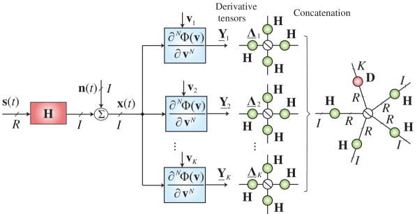
Figure 1.4: Tensorization based on derivatives of the characteristic functions and tensor-based approach to blind identification. The task is to estimate the mixing matrix, ${\bf H}$, from only the knowledge of the noisy output observations ${\bf X}=[{\bf x}(1),\ldots,{\bf x}(t),\ldots,{\bf x}(T)]\in\mathbb{R}^{I\times T}$, with $I<T$. A high dimensional tensor $\underline{\mathbf{Y}}$ is generated from the observations ${\bf X}$ by means of higher-order statistics (cumulants) or partial derivatives of the second generalised characteristic functions of the observations. A CP decomposition of $\underline{\mathbf{Y}}$ allows us to retrieve the mixing matrix ${\bf H}$.

A well-known approach to this problem is based on the decomposition of a high dimensional structured tensor, $\underline{\mathbf{Y}}$, generated from the observations, ${\bf X}$, by means of partial derivatives of the second GCFs of the observations at multiple processing points.

Derivatives of the GCFs. More specifically, we next show how to generate the tensor $\underline{\mathbf{Y}}$ from the observation, ${\bf X}$. We shall denote the first and second GCFs of the observations evaluated at a vector ${\bf u}$ of length $I$, respectively by

$$\phi_{{\bf x}}({\bf u})=\mbox{E}\left[\exp({\bf u}^{\text{T}}{\bf x})\right],\quad\Phi_{{\bf x}}({\bf u})=\log{\phi_{{\bf x}}({\bf u})}\,.$$ (1.133)

Similarly, $\phi_{{\bf s}}({\bf v})$ and $\Phi_{{\bf s}}({\bf v})$ designate the first and second GCFs of the sources, where ${\bf v}$ is of length $R$. Because the sources are statistically independent, the following holds

$$\Phi_{{\bf s}}({\bf v})=\Phi_{s_{1}}(v_{1})+\Phi_{s_{2}}(v_{2})+\cdots+\Phi_{s_{R}}(v_{R})\,,$$ (1.134)

which implies that $N$th-order derivatives of $\Phi_{{\bf s}}({\bf v})$ with respect to ${\bf v}$ result in $N$th-order diagonal tensors of size $R\times R\times\cdots\times R$, where $N=2,3,\ldots$, that is

$$\underline{\mathbf{\Psi}}_{{\bf s}}({\bf v})=\frac{\partial^{N}\Phi_{{\bf s}}({\bf v})}{\partial{\bf v}^{N}}=\mathop{\rm diag}\nolimits_{N}\!\left\{\frac{d^{N}\Phi_{s_{1}}}{dv_{1}^{N}},\frac{d^{N}\Phi_{s_{2}}}{dv_{2}^{N}},\ldots,\frac{d^{N}\Phi_{s_{R}}}{dv_{R}^{N}}\right\}\!.$$ (1.135)

In addition, for the noiseless case ${\bf x}(t)={\bf H}\,{\bf s}(t)$, and since $\Phi_{{\bf x}}({\bf u})=\Phi_{{\bf s}}({\bf H}^{\text{T}}{\bf u})$, the $N$th-order derivative of $\Phi_{{\bf x}}({\bf u})$ with respect to ${\bf u}$ yields a symmetric tensor of $N$th-order which admits a CP decomposition of rank-$R$ with $N$ identical factor matrices ${\bf H}$, to give

$$\underline{\mathbf{\Psi}}_{{\bf x}}({\bf u})=\underline{\mathbf{\Psi}}_{{\bf s}}({\bf H}^{\text{T}}{\bf u})\times_{1}{\bf H}\times_{2}{\bf H}\cdots\times_{N}{\bf H}\,.$$ (1.136)

In order to improve the identification accuracy, the mixing matrix ${\bf H}$ should be estimated as a joint factor matrix in decompositions of various derivative tensors, evaluated at distinct processing points ${\bf u}_{1}$, ${\bf u}_{2}$, …, ${\bf u}_{K}$. This is equivalent to a decomposition of an $(N+1)$th-order tensor $\underline{\mathbf{Y}}$ of size $I\times I\times\cdots\times I\times K$ concatenated from the $K$ derivative tensors as

$$\underline{\mathbf{Y}}(:,\ldots,:,k)=\underline{\mathbf{\Psi}}_{{\bf x}}({\bf u}_{k}),\quad k=1,2,\ldots,K.$$ (1.137)

The CP decomposition of the tensor $\underline{\mathbf{Y}}$ can be written in form of

$$\underline{\mathbf{Y}}=\underline{\mathbf{I}}\times_{1}{\bf H}\times_{2}{\bf H}\cdots\times_{N}{\bf H}\times_{N+1}{\bf D}\,,$$ (1.138)

where the last factor matrix ${\bf D}$ is of size $K\times R$, and each row comprises the diagonal of the symmetric tensor $\underline{\mathbf{\Psi}}_{{\bf s}}({\bf H}^{\text{T}}{\bf u}_{k})$.

In the presence of statistically independent, additive and stationary Gaussian noise, we can eliminate the derivatives of the noise terms in the derivative tensor $\underline{\mathbf{\Psi}}_{{\bf x}}({\bf u})$ by subtracting any other derivative tensor $\underline{\mathbf{\Psi}}_{{\bf x}}(\tilde{{\bf u}})$, or by an average of derivative tensors.

Estimation of Derivatives of GCF. In practice, the GCF of the observation and its derivatives are unknown, but can be estimated from the sample first GCF [Yeredor, 2000]. Detailed expression and the approximation of the derivative tensor $\underline{\mathbf{\Psi}}_{{\bf x}}({\bf u})$ for some low orders $N=2,3,\ldots,7$, are given in Appendix 1.

Cumulants. When the derivative is taken at the origin, ${\bf u}=[0,\ldots,0]^{\text{T}}$, the tensor ${\mathcal{K}}_{{\bf x}}^{(N)}=\underline{\mathbf{\Psi}}_{{\bf x}}^{(N)}({\bf 0})$ is known as the $N$th-order cumulant of ${\bf x}$, and a joint diagonalization or the CP decomposition of higher-order cumulants is a well-studied method for the estimation of the mixing matrix ${\bf H}$.

For the sources with symmetric probabilistic distributions, their odd-order cumulants, $N=3,5,\ldots$, are zero, and the cumulants of the mixtures are only due to noise. Hence, a decomposition of such tensors is not able to retrieve the mixing matrix. However, the odd-order cumulant tensors can be used to subtract the noise term in the derivative tensors evaluated at other processing points.

Example 6  Blind identification (BI) in a system of $2$ mixtures and $R$ binary signals.

To illustrate the efficiency of higher-order derivatives of the second GCF in blind identification we considered a system of two mixtures, $I=2$, linearly composed by $R$ signals of length $T=100\times\,2^{R}$, the entries of which can take the values 1 or $-1$, i.e., $s_{r,t}=1$ or $-1$. The mixing matrix ${\bf H}$ of size $2\times R$ was randomly generated, where $R=4,6,8$. The signal-to-noise ratio was SNR = 20 dB. The main purpose of BI is to estimate the mixing matrix ${\bf H}$.

We constructed 50 tensors $\underline{\mathbf{Y}}_{i}$ $\;(i=1,\ldots,50)$ of size $R\times\cdots\times R\times 3$, which comprise three derivative tensors evaluated at the two leading left singular vectors of ${\bf X}$, and a unit-length processing point, generated such that its collinearity degree with the first singular vector uniformly distributed over a range of $[-0.99,0.99]$. The average derivative tensor was used to eliminate the noise term in $\underline{\mathbf{Y}}_{i}$.

CP decomposition of derivative tensors. The tensors $\underline{\mathbf{Y}}_{i}$ were decomposed by CP decompositions of rank-$R$ to retrieve the mixing matrix ${\bf H}$. The mean of Squared Angular Errors $SAE({\bf h}_{r},\hat{{\bf h}}_{r})=-20\log_{10}\arccos(\frac{{\bf h}_{r}^{\text{T}}\hat{{\bf h}}_{r}}{|{\bf h}_{r}|_{2}|\hat{{\bf h}}_{r}|_{2}})$ over all columns ${\bf h}_{r}$ was computed as a performance index for one estimation of the mixing matrix.

The averages of the mean and best MSAEs over 100 independent runs for the number of the unknown sources $R=4,6,8$ are plotted in Figure 1.5. The results indicate that with a suitably chosen processing point, the decomposition of the derivative tensors yielded good estimation of the mixing matrix. Of more importance is that higher-order derivative tensors, e.g., 7th and 8th orders, yielded better performance than lower-order tensors, while the estimation accuracy deteriorated with the number of sources.

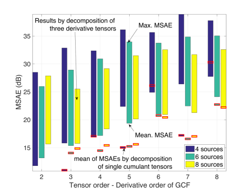
Figure 1.5: Mean SAE (in dB) in the estimation of the mixing matrix ${\bf H}$ from only two mixtures, achieved by CP decomposition of three $2\times 2\times\cdots\times 2$ derivative tensors of the second GCFs. Small bars in red represent the mean of MSAEs, obtained by decomposition of single cumulant tensors.

CP decomposition of cumulant tensors. Because of symmetric pdfs, the odd order cumulants of the sources are zero. Only decompositions of cumulants of order 6 or 8 were able to retrieve the mixing matrix ${\bf H}$. For all the test cases, better performances could be obtained by a decomposition of three derivative tensors.

Tensor train decomposition of derivative tensors. The estimation of the mixing matrix ${\bf H}$ can be performed in a two-stage decomposition

• A tensor train decomposition of high-order derivative tensors, e.g., tensor order exceeds 5.

• A CP decomposition of the tensor in TT-format, to retrieve the mixing matrix.

Experimental results confirmed that the performances with prior TT-decomposition were more stable and yielded an approximately 2 dB higher mean SAE than those using only CP decomposition for derivative tensors of orders 7 and 8 and a relatively high number of unknown sources.

1.4.1 Tensor Structures in Constant Modulus Signal Separation

Another method to generate tensors of relatively high order in BSS is through modelling modulus of the estimated signals as roots of a polynomial.

Consider a linear mixing system ${\bf X}={\bf H}{\bf S}$ with $R$ sources of length $K$, and $I$ mixtures, where the modulus of the sources ${\bf S}$ is drawn from a set of given moduli. For simplicity, we assume $I=R$. For example, the binary phase-shift keying (BPSK) signal in telecommunication consists of a sequence of 1 and $-1$, hence, it has a constant modulus of unity. The quadrature phase shift keying (QPSK) signal takes one of the values $\pm 1\pm 1i$, i.e., it has a constant modulus $\sqrt{2}$. The 16-QAM signal has three squared moduli of 2, 10 and 18. For this BSS problem for single constant modulus signals, Lathauwer [2004] linked the problem to CP decomposition of a fourth-order tensor. For multi-constant modulus signals, Debals et al. [2016b] established a link to a coupled CP decomposition.

A common method to extract the original sources ${\bf S}$ is to use a demixing matrix ${\bf W}$ of size $I\times R$ or a vector ${\bf w}$ of length $I$ such that ${\bf y}={\bf w}^{\text{T}}{\bf X}$ is an estimate of one of the source signals. The constant modulus constraints require that each entry, $|y_{k}|$, must be one of given moduli, $c_{1},c_{2},\ldots,c_{M}$. This means that for all entries of ${\bf y}$ the following holds

$$f(y_{k})=\prod_{m=1}^{M}(|y_{k}|^{2}-c_{m})=0\,.$$ (1.139)

In other words, $|y_{k}|^{2}$ are roots of an $M$th-degree polynomial, given by

$$p^{M}+\alpha_{m}p^{M-1}+\cdots+\alpha_{2}p+\alpha_{1}\,,$$

with coefficients $\alpha_{M+1}=1$, and $\alpha_{1},\alpha_{2},\ldots,\alpha_{M}$, given by

$$\alpha_{m}=(-1)^{m-1}\sum_{i_{1},i_{2},\ldots,i_{m}}c_{i_{1}}c_{i_{2}}\cdots c_{i_{m}}\,.$$ (1.140)

By expressing $|y_{k}|^{2}=({\bf w}\otimes{\bf w}^{*})^{\text{T}}({\bf x}_{k}\otimes{\bf x}_{k}^{*})$, and

$$|y_{k}|^{2m}=({\bf w}^{\otimes_{m}}\otimes({\bf w}^{\otimes_{m}})^{*})^{\text{T}}({\bf x}_{k}^{\otimes_{m}}\otimes({\bf x}_{k}^{\otimes_{m}})^{*})\,,$$

where the symbol “$*$” represents the complex conjugate, ${\bf x}^{\otimes_{m}}={\bf x}\otimes{\bf x}\otimes\cdots\otimes{\bf x}$ denotes the Kronecker product of $m$ vectors ${\bf x}$, and bearing in mind that the rank-1 tensors ${\bf w}^{\circ_{m}}={\bf w}\circ{\bf w}\circ\cdots\circ{\bf w}$ are symmetric, and in general have only $\frac{(R+m-1)!}{m!(R-1)!}$ distinct coefficients, the rank-1 tensors ${\bf w}^{\circ_{m}}\circ({\bf w}^{\circ_{m}})^{*}$ have at least $\left(\frac{(R+m-1)!}{m!(R-1)!}\right)^{2}$ distinct entries. We next introduce the operator ${\mathcal{K}}$ which keeps only distinct entries of the symmetric tensor ${\bf w}^{\circ_{m}}\circ({\bf w}^{\circ_{m}})^{*}$ or of the vector ${\bf w}^{\otimes_{m}}\otimes({\bf w}^{\otimes_{m}})^{*}$. The constant modulus constraint of $y_{k}$ can then be rewritten as

$$f(y_{k}) =\alpha_{1}+\sum_{m=2}^{M+1}\!\!\alpha_{m}({\bf w}^{\otimes_{m}}\otimes({\bf w}^{\otimes_{m}})^{*})^{\text{T}}({\bf x}_{k}^{\otimes_{m}}\otimes({\bf x}_{k}^{\otimes_{m}})^{*})$$

$$=\alpha_{1}+\sum_{m=2}^{M+1}\!\!\alpha_{m}({\mathcal{K}}({\bf w}^{\otimes_{m}}\otimes({\bf w}^{\otimes_{m}})^{*}))^{\text{T}}\mathop{\rm diag}\nolimits({\bf d}_{m})\,{\mathcal{K}}({\bf x}_{k}^{\otimes_{m}}\otimes({\bf x}_{k}^{\otimes_{m}})^{*})$$

$$=\alpha_{1}+\left[\ldots,({\mathcal{K}}({\bf w}^{\otimes_{m}}\otimes({\bf w}^{\otimes_{m}})^{*}))^{\text{T}},\ldots\right]$$

$$\qquad\qquad[\ldots,{\mathcal{K}}({\bf x}_{k}^{\otimes_{m}}\otimes({\bf x}_{k}^{\otimes_{m}})^{*})^{\text{T}}\mathop{\rm diag}\nolimits(\alpha_{m}{\bf d}_{m}),\ldots]^{\text{T}}\,,$$

where $d_{m}(i)$ represents the number of occurrences of an entry of ${\mathcal{K}}({\bf x}_{k}^{\otimes_{m}}\otimes({\bf x}_{k}^{\otimes_{m}})^{*})$ in ${\bf x}_{k}^{\otimes_{m}}\otimes({\bf x}_{k}^{\otimes_{m}})^{*}$.

The vector of the constant modulus constraints of ${\bf y}$ is now given by

$$\boldsymbol{f} = [\ldots,f(y_{k}),\ldots]^{\text{T}}=\alpha_{1}{\bf 1}+{\bf Q}{\bf v}\,,$$ (1.141)

where

$${\bf v}=\left[\begin{array}[]{@{}c@{}}\vdots\\ {\mathcal{K}}({\bf w}^{\otimes_{m}}\otimes({\bf w}^{\otimes_{m}})^{*})\\ \vdots\end{array}\right],\;{\bf Q}=\left[\begin{array}[]{@{}c@{}}\vdots\\ \mathop{\rm diag}\nolimits(\alpha_{m}{\bf d}_{m}){\mathcal{K}}({\bf X}^{\odot_{m}}\odot({\bf X}^{\odot_{m}})^{*})\\ \vdots\end{array}\right]^{\text{T}}\!.$$ (1.148)

The constraint vector is zero for the exact case, and should be small for the noisy case. For the exact case, from (1.141) and $f(y_{k+1})-f(y_{k})=0$, this leads to

$${\bf L}{\bf Q}{\bf v}={\bf 0}\,,$$

where ${\bf L}$ is the first-order Laplacian implying that the vector ${\bf v}$ is in the null space of the matrix $\tilde{{\bf Q}}={\bf L}{\bf Q}$. The above condition holds for other demixing vectors ${\bf w}$, i.e., $\tilde{{\bf Q}}{\bf V}={\bf 0}$, where ${\bf V}=[{\bf v}_{1},\ldots,{\bf v}_{R}]$, and each ${\bf v}_{r}$ is constructed from a corresponding demixing vector ${\bf w}_{r}$.

With the assumption $I=R$, and that the sources have complex values, and the mixing matrix does not have collinear columns, it can be shown that the kernel of the matrix $\tilde{{\bf Q}}$ has the dimension of $R$ [Debals et al., 2016b]. Therefore, the basis vectors, ${\bf z}_{r}$, $r=1,\ldots,R$, of the kernel of $\tilde{{\bf Q}}$ can be represented as linear combination of ${\bf V}$, that is

$${\bf z}_{r}={\bf V}\mbox{\boldmath$\lambda$}_{r}\,.$$

Next we partition ${\bf z}_{r}$ into $M$ parts, ${\bf z}_{r}=[{\bf z}_{rm}]$, each of the length $\left(\frac{(R+m-1)!}{m!(R-1)!}\right)^{2}$, which can be expressed as

$${\bf z}_{rm}=\sum_{s=1}^{R}\lambda_{rs}{\mathcal{K}}({\bf w}_{s}^{\otimes_{m}}\otimes({\bf w}_{s}^{\otimes_{m}})^{*})={\mathcal{K}}\left(\sum_{s=1}^{R}\lambda_{rs}{\bf w}_{s}^{\otimes_{m}}\otimes({\bf w}_{s}^{\otimes_{m}})^{*}\right),$$

thus implying that ${\bf W}$ and ${\bf W}^{*}$ are factor matrices of a symmetric tensor $\underline{\mathbf{Z}}_{rm}$ of $(2m)$th-order, constructed from the vector ${\bf z}_{rm}$, i.e., ${\mathcal{K}}(\operatorname{vec}\left(\underline{\mathbf{Z}}_{rm}\right))={\bf z}_{rm}$, in the form

$$\underline{\mathbf{Z}}_{rm}=\llbracket\mathop{\rm diag}\nolimits_{2m}(\mbox{\boldmath$\lambda$}_{r});\underbrace{{\bf W},\ldots,{\bf W}}_{\text{$m$ terms}},\underbrace{{\bf W}^{*},\ldots,{\bf W}^{*}}_{\text{$m$ terms}}\rrbracket\,.$$ (1.149)

By concatenating all $R$ tensors $\underline{\mathbf{Z}}_{1m}$, …, $\underline{\mathbf{Z}}_{Rm}$ into one $(2m+1)$th-order tensor $\underline{\mathbf{Z}}_{m}$, the above $R$ CP decompositions become

$$\underline{\mathbf{Z}}_{m}=\llbracket\underline{\mathbf{I}};\underbrace{{\bf W},\ldots,{\bf W}}_{\text{$m$ terms}},\underbrace{{\bf W}^{*},\ldots,{\bf W}^{*}}_{\text{$m$ terms}},\mbox{\boldmath$\Lambda$}\rrbracket\,.$$ (1.150)

All together, the $M$ CP decompositions of $\underline{\mathbf{Z}}_{1}$, …, $\underline{\mathbf{Z}}_{M}$ form a coupled CP tensor decomposition to find the two matrices ${\bf W}$ and $\Lambda$.

Example 7  [Separation of QAM signals.]

We performed the separation of two rectangular 32- or 64-QAM signals of length $1000$ from two mixture signals corrupted by additive Gaussian noise with SNR = 15 dB. Columns of the real-valued mixing matrix had unit-length, and a pair-wise collinearity of 0.4. The 32-QAM signal had $M=5$ constant moduli of 2, 10, 18, 26 and 34, whereas the 64-QAM signal had $M=9$ squared constant moduli of 2, 10, 18, 26, 34, 50, 58, 74 and 98. Therefore, for the first case (32-QAM), the demixing matrix was estimated from 5 tensors of size $2\times 2\times\cdots\times 2$ and of respective orders 3, 5, 7, 9 and 11, while for the later case (64-QAM), we decomposed 9 quantized tensors of orders 3, 5, …, 19. The estimated QAM signals for the two cases were perfectly reconstructed with zero bit error rates. Scatter plots of the recovered signals are shown in Figure 1.6.

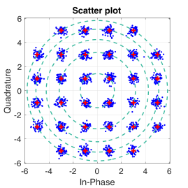
(a) 32-QAM

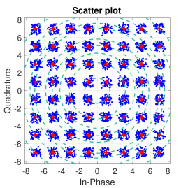
(b) 64-QAM

Figure 1.6: Scatter plots of the estimated sources (blue dots). Red dots indicate the ideal signal constellation, the values of which are located on one of dashed circles.

1.5 Tensorization by Learning Local Structures

Different from the previous tensorizations, this tensorization approach generates tensors from local blocks (patches) which are similar or closely related. For the example of an image, given that the intensities of pixels in a small window are highly correlated, hidden structures which represent relations between small patches of pixels can be learnt in local areas. These structures can then be used to reconstruct the image as a whole in, e.g., an application of image denoising [Phan et al., 2016].

Figure 1.7: A “local-structure” tensorization method generates 5th-order tensors of size $h\times w\times 3\times(2d+1)\times(2d+1)$ from similar image patches, or patches in close spatial proximity.

For a color RGB image $\underline{\mathbf{Y}}$ of size $I\times J\times 3$, each block of pixels of size $h\times w\times 3$ is denoted as

$$\underline{\mathbf{Y}}_{r,c}=\underline{\mathbf{Y}}(r:r+h-1,c:c+w-1,:).$$

A small tensor, $\underline{\mathbf{Z}}_{r,c}$, of size $h\times w\times 3\times(2d+1)\times(2d+1)$, comprising $(2d+1)^{2}$ blocks centered around $\underline{\mathbf{Y}}_{r,c}$, with $d$ denoting the neighbourhood width, can be constructed in the form

$$\underline{\mathbf{Z}}_{r,c}(:,:,:,d+1+i,d+1+j)=\underline{\mathbf{Y}}_{r+i,c+j},$$

where $i,j=-d,\ldots,0,\ldots,d$, as illustrated in Figure 1.7. Every $(r,c)$-th block $\underline{\mathbf{Z}}_{r,c}$ is then approximated through a constrained tensor decomposition

$$\|\underline{\mathbf{Z}}_{r,c}-\hat{\underline{\mathbf{Z}}}_{r,c}\|_{F}^{2}\leq\varepsilon^{2}\,,$$ (1.151)

where the noise level $\varepsilon^{2}$ can be determined by inspecting the coefficients of the image in the high-frequency bands. A pixel is then reconstructed as the average of all its approximations which cover that pixel.

Example 8  Image denoising. The principle of tensorization from learning the local structures is next demonstrated in an image denoising application for the benchmark “peppers” color image of size $256\times 256\times 3$, which was corrupted by white Gaussian noise at SNR = 10 dB. Latent structures were learnt for patches of sizes $8\times 8\times 3$ (i.e., $h=w=8$) in the search area of width $d=3$. To the noisy image, we applied the DCT spatial filtering before their block reconstruction. The results are shown in Figure 1.8, and illustrate the advantage of the tensor network approach over a CP decomposition approach.

(a) Noisy image

(b) TT, PSNR = 31.64 dB

(c) CP, PSNR = 28.90 dB

Figure 1.8: Tensor based image reconstruction in Example 1.5. The Pepper image with added noise at 10 dB SNR (left), and the images reconstructed using the TT (middle) and CP (right) decompositions.

1.6 Tensorization based on Divergences, Similarities or Information Exchange

For a set of $I$ data points ${\bf x}_{i}$, $i=1,2,\ldots,I$, this type of tensorization generates an $N$th-order nonnegative symmetric tensor of size $I\times I\times\cdots\times I$, the entries of which represent $N$-way similarities or dissimilarities between ${\bf x}_{i_{1}}$, ${\bf x}_{i_{2}}$, …, ${\bf x}_{i_{N}}$, where $i_{n}=1,\ldots,I$, so that

$$\underline{\mathbf{Y}}(i_{1},i_{2},\ldots,i_{N})=d({\bf x}_{i_{1}},{\bf x}_{i_{2}},\ldots,{\bf x}_{i_{N}})\,.$$ (1.152)

Such metric function can express pair-wise distances between the two observations ${\bf x}_{i}$ and ${\bf x}_{j}$. In a general case, $d({\bf x}_{i_{1}},{\bf x}_{i_{2}},\ldots,{\bf x}_{i_{N}})$ can compute the volume of a convex hull formed by $N$ data points.

The so generated tensor can be expanded to $(N+1)$th-order tensor, where the last mode expresses the change of data points over e.g., time or trials. Tensorizations based on divergences and similarities are useful for the analysis of interaction between observed entities, and for their clustering or classification.

1.7 Tensor Structures in Multivariate Polynomial Regression

The Multivariate Polynomial Regression (MPR) is an extension of the linear and multilinear regressions which allows us to model nonlinear interaction between independent variables [Chen and Billings, 1989, Billings, 2013, Vaccari, 2003]. For illustration, consider a simple example of fitting a curve to data with two independent variables $x_{1}$ and $x_{2}$, in the form

$$y = w_{0}+w_{1}x_{1}+w_{2}x_{2}+w_{12}x_{1}x_{2}\,.$$ (1.153)

The term $w_{12}$ then quantifies the strength of interaction between the two independent variables in the data, $x_{1}$ and $x_{2}$. Observe that the model is still linear with respect to the variables $x_{1}$ and $x_{2}$, while involving the cross-term $w_{12}x_{1}x_{2}$. The above model can also have more terms, e.g., $x_{1}^{2},x_{1}x_{2}^{2}$, to describe more complex functional behaviours. For example, the full quadratic polynomial regression for two independent variables, $x_{1}$ and $x_{2}$, can have up to 9 terms, given by

$$y = w_{0}+w_{1}x_{1}+w_{2}x_{2}+w_{12}x_{1}x_{2}$$ (1.154)

$$+w_{11}x_{1}^{2}+w_{22}x_{2}^{2}+w_{112}x_{1}^{2}x_{2}+w_{122}x_{1}x_{2}^{2}+w_{1122}x_{1}^{2}x_{2}^{2}\,.\;\;\;\;$$

Tensor representation of the system weights. The simple model for two independent variables in (1.153) can be rewritten in a bilinear form as

$$y=\left[\begin{array}[]{cc}1&x_{1}\end{array}\right]\,\left[\begin{array}[]{cc}w_{0}&w_{2}\\ w_{1}&w_{12}\end{array}\right]\left[\begin{array}[]{c}1\\ x_{2}\end{array}\right]\,,$$ (1.160)

whereas the full model in (1.154) has an equivalent bilinear expression

$$y = \left[\begin{array}[]{ccc}1&x_{1}&x_{1}^{2}\end{array}\right]\,\left[\begin{array}[]{ccc}w_{0}&w_{2}&w_{22}\\ w_{1}&w_{12}&w_{122}\\ w_{11}&w_{112}&w_{1122}\end{array}\right]\left[\begin{array}[]{c}1\\ x_{2}\\ x_{2}^{2}\end{array}\right]\,,$$ (1.168)

or a tensor-vector product representation

$$y=\underline{\mathbf{W}}\,{\bar{\times}_{1}}\,\left[\begin{array}[]{c}1\\ x_{1}\end{array}\right]\,{\bar{\times}_{2}}\,\left[\begin{array}[]{c}1\\ x_{1}\end{array}\right]\,{\bar{\times}_{3}}\,\left[\begin{array}[]{c}1\\ x_{2}\end{array}\right]\,{\bar{\times}_{4}}\,\left[\begin{array}[]{c}1\\ x_{2}\end{array}\right]\,,$$ (1.177)

where the 4th-order weight tensor $\underline{\mathbf{W}}$ is of size $2\times 2\times 2\times 2$, and is given by

$$\underline{\mathbf{W}}(:,:,1,1) =\left[\begin{array}[]{cc}w_{0}&\frac{1}{2}w_{1}\\ \frac{1}{2}w_{1}&w_{11}\end{array}\right],\;\;\underline{\mathbf{W}}(:,:,2,2)=\left[\begin{array}[]{cc}w_{22}&\frac{1}{2}w_{122}\\ \frac{1}{2}w_{122}&w_{1122}\end{array}\right]\,,$$ (1.182)

$$\underline{\mathbf{W}}(:,:,1,2) =\underline{\mathbf{W}}(:,:,2,1)=\frac{1}{2}\left[\begin{array}[]{cc}w_{2}&\frac{1}{2}w_{12}\\ \frac{1}{2}w_{12}&w_{112}\end{array}\right]\,.\;\;$$ (1.185)

It is now obvious that for a generalised system with $N$ independent variables, $x_{1}$, …, $x_{N}$, the MPR can be written as a tensor-vector product as [Chen and Billings, 1989]

$$y = \sum_{i_{1}=0}^{N}\sum_{i_{2}=0}^{N}\cdots\sum_{i_{N}=0}^{N}w_{i_{1},i_{2},\ldots,i_{N}}\,x_{1}^{i_{1}}\,x_{2}^{i_{2}}\cdots\,x_{N}^{i_{N}}\,$$ (1.186)

$$= \underline{\mathbf{W}}\,\bar{\times}_{1}\,{\mathcal{V}}_{N}(x_{1})\,\bar{\times}_{2}\,{\mathcal{V}}_{N}(x_{2})\,\cdots\,\bar{\times}_{N}\,{\mathcal{V}}_{N}(x_{N})\,,$$

where $\underline{\mathbf{W}}$ is an $N$th-order tensor of size $(N+1)\times(N+1)\times\cdots\times(N+1)$, and ${\mathcal{V}}_{N}(x)$ is the length-$(N+1)$ Vandermonde vector of $x$, given by

$${\mathcal{V}}_{N}(x)=\left[\begin{array}[]{ccccc}1&x&x^{2}&\ldots&x^{N}\end{array}\right]^{\text{T}}\,.$$ (1.188)

Similarly to the representation in (1.177), the MPR model in (1.186) can be equivalently expressed as a product of a tensor of $N^{2}$th-order and size $2\times 2\times\cdots\times 2$ with $N$ vectors of length-2, to give

$$y=\widetilde{\underline{\mathbf{W}}}\,\bar{\times}_{1:N}\left[\begin{array}[]{c}1\\ x_{1}\end{array}\right]\,\bar{\times}_{N+1:2N}\left[\begin{array}[]{c}1\\ x_{2}\end{array}\right]\,\cdots\bar{\times}_{N(N-1)+1:N^{2}}\left[\begin{array}[]{c}1\\ x_{N}\end{array}\right]\,.\;\;\;$$ (1.195)

An illustration of the MPR is given in Figure 1.9, where the input units are scalars.

(a)                                                      (b)

Figure 1.9: Graphical illustration of Multivariate Polynomial Regression (MPR). (a) The MPR for multiple input units $x_{1}$, …, $x_{N}$, where the nonlinear function $h(x_{1},\ldots,x_{N})$ is expressed as a multilinear tensor-vector product of an $N$th-order tensor, $\underline{\mathbf{W}}$, of size $(N+1)\times(N+1)\times\cdots\times(N+1)$, and Vandermonde vectors ${\mathcal{V}}_{N}(x_{n})$ of length $(N+1)$. (b) An equivalent MPR model but with quantized $N^{2}$th-order tensor $\widetilde{\underline{\mathbf{W}}}$ of size $2\times 2\times\cdots\times 2$.

The MPR has found numerous applications, owing to its ability to model any smooth, continuous nonlinear input-output system , see e.g. [Vaccari, 2003]. However, since the number of parameters in the model in (1.186) grows exponentially with the number of variables, $N$, the MPR demands a huge amount of data in order to yield a good model, and therefore, it is computationally intensive in a raw tensor format, and thus not suitable for very high-dimensional data. To this end, low-rank tensor network representation emerges as a viable approach to accomplishing MPR. For example, the weight tensor $\underline{\mathbf{W}}$ can be constrained to be in low rank TT-format [Chen et al., 2016]. An alternative approach would be to consider a truncated model which takes only two entries along each mode of $\underline{\mathbf{W}}$ in (1.186). In other words, this truncated model becomes linear with respect to each variable $x_{n}$ [Novikov et al., 2016], leading to

$$y = \underline{\mathbf{W}}_{t}\,\bar{\times}_{1}\,\left[\begin{array}[]{c}1\\ x_{1}\end{array}\right]\,\bar{\times}_{2}\,\left[\begin{array}[]{c}1\\ x_{2}\end{array}\right]\,\cdots\bar{\times}_{N}\,\left[\begin{array}[]{c}1\\ x_{N}\end{array}\right]\,,$$ (1.202)

where $\underline{\mathbf{W}}_{t}$ is a tensor of size $2\times 2\times\cdots\times 2$ in the QTT-format. Both (1.195) and (1.202) represent the weight tensors in the QTT-format, however, the tensor $\widetilde{\underline{\mathbf{W}}}$ in (1.195) has $N^{2}$ core tensors of the full MPR, whereas $\underline{\mathbf{W}}_{t}$ in (1.202) has $N$ core tensors for the truncated model.

1.8 Tensor Structures in Vector-variate Regression

The MPR in (1.186) is formulated for scalar data. When the observations are vectors or tensors, the model can be extended straightforwardly. For illustration, consider a simple case of two independent vector inputs ${\bf x}_{1}$ and ${\bf x}_{2}$. Then, the nonlinear function which maps the input to the output $y=h({\bf x}_{1},{\bf x}_{2})$ can be approximated in a linear form as

$$y=h({\bf x}_{1},{\bf x}_{2}) =w_{0}+{\bf w}_{1}^{\text{T}}{\bf x}_{1}+{\bf w}_{2}^{\text{T}}{\bf x}_{2}+{\bf x}_{1}^{\text{T}}{\bf W}_{12}{\bf x}_{2}\,$$ (1.203)

$$=[1,\;{\bf x}_{1}^{\text{T}}]\,\left[\begin{array}[]{cc}w_{0}&{\bf w}_{2}^{\text{T}}\\ {\bf w}_{1}&{\bf W}_{12}\end{array}\right]\left[\begin{array}[]{cc}1\\ {\bf x}_{2}\end{array}\right],$$ (1.208)

or in a quadratic with 9 terms, including one bias, two vectors, three matrices, two third-order tensors and one fourth-order tensor, given by

$$h({\bf x}_{1},{\bf x}_{2}) =w_{0}+{\bf w}_{1}^{\text{T}}{\bf x}_{1}+{\bf w}_{2}^{\text{T}}{\bf x}_{2}+{\bf x}_{1}^{\text{T}}{\bf W}_{12}{\bf x}_{2}+{\bf x}_{1}^{\text{T}}\,{\bf W}_{11}{\bf x}_{1}+{\bf x}_{2}^{\text{T}}\,{\bf W}_{22}{\bf x}_{2}$$

$$+\underline{\mathbf{W}}_{112}\,\bar{\times}_{1}\,{\bf x}_{1}\,\bar{\times}_{2}\,{\bf x}_{1}\,\bar{\times}_{3}\,{\bf x}_{2}+\underline{\mathbf{W}}_{122}\,\bar{\times}_{1}\,{\bf x}_{1}\,\bar{\times}_{2}\,{\bf x}_{2}\,\bar{\times}_{3}\,{\bf x}_{2}$$

$$+\underline{\mathbf{W}}_{1122}\,\bar{\times}_{1}\,{\bf x}_{1}\,\bar{\times}_{2}\,{\bf x}_{1}\,\bar{\times}_{3}\,{\bf x}_{2}\,\bar{\times}_{4}\,{\bf x}_{2}$$

$$=[1,\;{\bf x}_{1}^{\text{T}},\;({\bf x}_{1}\otimes{\bf x}_{1})^{T}]\;{\bf W}\;\left[\begin{array}[]{cc}1\\ {\bf x}_{2}\\ {\bf x}_{2}\otimes{\bf x}_{2}\end{array}\right],$$ (1.212)

where the matrix ${\bf W}$ is given

$${\bf W}=\left[\begin{array}[]{ccc}w_{0}&{\bf w}_{2}^{\text{T}}&\operatorname{vec}\left({\bf W}_{22}\right)^{\text{T}}\\ {\bf w}_{1}&{\bf W}_{12}&[\underline{\mathbf{W}}_{122}]_{(1)}\\ \operatorname{vec}\left({\bf W}_{11}\right)&[\underline{\mathbf{W}}_{112}]_{(1,2)}&[\underline{\mathbf{W}}_{1122}]_{(1,2)}\end{array}\right]\,.$$ (1.216)

and $[\underline{\mathbf{W}}_{112}]_{(1,2)}$ represents the mode-(1,2) unfolding of the tensor $\underline{\mathbf{W}}_{112}$. Similarly to (1.177), the above model has an equivalent expression of through the tensor-vector product of a fourth-order tensor $\underline{\mathbf{W}}$, in the form

$$y=\underline{\mathbf{W}}\,{\bar{\times}_{1}}\,\left[\begin{array}[]{c}1\\ {\bf x}_{1}\end{array}\right]\,{\bar{\times}_{2}}\,\left[\begin{array}[]{c}1\\ {\bf x}_{1}\end{array}\right]\,{\bar{\times}_{3}}\,\left[\begin{array}[]{c}1\\ {\bf x}_{2}\end{array}\right]\,{\bar{\times}_{4}}\,\left[\begin{array}[]{c}1\\ {\bf x}_{2}\end{array}\right]\,.$$ (1.225)

In general, the regression for a system with $N$ input vectors, ${\bf x}_{n}$ of lengths $I_{n}$, can be written as

$$h({\bf x}_{1},\ldots,{\bf x}_{N})=w_{0}+\sum_{d=1}^{N^{2}}\sum_{i_{1},i_{2},\ldots,i_{d}=1}^{N}\underline{\mathbf{W}}_{i_{1},i_{2},\ldots,i_{d}}\bar{\times}\,({\bf x}_{i_{1}}\circ{\bf x}_{i_{2}}\,\circ\cdots\circ{\bf x}_{i_{d}})\,,$$ (1.226)

where $\bar{\times}$ represents the inner product between two tensors, and the tensors $\underline{\mathbf{W}}_{i_{1},\ldots,i_{d}}$ are of $d$-th order, and of size $I_{i_{1}}\times I_{i_{2}}\times\cdots\times I_{i_{d}}$, $d=1,\ldots,N^{2}$. The representation of the generalised model as a tensor-vector product of an $N$th-order tensor of size $J_{1}\times J_{2}\times\cdots\times J_{N}$, where $J_{n}=\frac{I_{n}^{N+1}-1}{I_{n}-1}$, comprising all the weights, is given by

$$h({\bf x}_{1},\ldots,{\bf x}_{N})=\underline{\mathbf{W}}\,\bar{\times}_{1}\,{\bf v}_{N}({\bf x}_{1})\,\bar{\times}_{2}\,{\bf v}_{N}({\bf x}_{2})\,\cdots\,\bar{\times}_{N}\,{\bf v}_{N}({\bf x}_{N}),$$ (1.227)

where

$${\bf v}_{N}({\bf x})=\left[\begin{array}[]{ccccc}1&{\bf x}^{\text{T}}&({\bf x}\otimes{\bf x})^{T}&\ldots&({\bf x}\otimes\cdots\otimes{\bf x})^{T}\end{array}\right]^{\text{T}}\,,$$ (1.229)

or, in a more compact form, with a very high-order tensor $\widetilde{\underline{\mathbf{W}}}$ of $N^{2}$th-order and of size $(I_{1}+1)\times\cdots\times(I_{1}+1)\times(I_{2}+1)\times\cdots\times(I_{N}+1)\times\cdots\times(I_{N}+1)$, as

$$h({\bf x}_{1},\ldots,{\bf x}_{N})=\widetilde{\underline{\mathbf{W}}}\,\bar{\times}_{1:N}\,\left[\begin{array}[]{c}1\\ {\bf x}_{1}\end{array}\right]\,\cdots\bar{\times}_{N(N-1)+1:N^{2}}\,\left[\begin{array}[]{c}1\\ {\bf x}_{N}\end{array}\right]\,.$$ (1.234)

The illustration of this generalized model is given in Figure 1.10.

(a)                                                      (b)

Figure 1.10: Graphical illustration of the vector-variate regression. (a) The vector-variate regression for multiple input units ${\bf x}_{1}$, …, ${\bf x}_{N}$, where the nonlinear function $h({\bf x}_{1},\ldots,{\bf x}_{N})$ is expressed as a tensor-vector product of an $N$th-order core tensor, $\underline{\mathbf{W}}$, of size $J_{1}\times J_{2}\times\cdots\times J_{N}$, and Vandermonde-like vectors ${\bf v}_{N}({\bf x}_{n})$ of length $J_{n}$, where $J_{n}=\frac{I_{n}^{N+1}-1}{I_{n}-1}$. (b) An equivalent regression model but with an $N^{2}$th-order tensor of size $(I_{1}+1)\times\cdots\times(I_{1}+1)\times(I_{2}+1)\times\cdots\times(I_{N}+1)\times\cdots\times(I_{N}+1)$. When the input units are scalars, the tensor $\widetilde{\underline{\mathbf{W}}}$ is of size $2\times 2\times\cdots\times 2$.

Tensor-variate model. When the observations are matrices, ${\bf X}_{n}$, or higher-order tensors, $\underline{\mathbf{X}}_{n}$, the models in (1.226), (1.227) and (1.234) are still applicable and operate by replacing the original vectors, ${\bf x}_{n}$, by the vectorization of the higher-order inputs. This is because the inner product between two tensors can be expressed as a product of their two vectorizations.

Separable representation of the weights. Similar to the MPR, the challenge in the generalised tensor-variate regression is the curse of dimensionality of the weight tensor $\underline{\mathbf{W}}$ in (1.227), or of the tensor $\widetilde{\underline{\mathbf{W}}}$ in (1.234).

A common method to deal with the problem is to restrict the model to some low order, i.e., to the first order. The weight tensor is now only of size $(I_{1}+1)\times(I_{2}+1)\times\cdots\times(I_{N}+1)$. The large weight tensor can then be represented in the canonical form [Nguyen et al., 2015, Qi et al., 2016], the TT/MPS tensor format [Stoudenmire and Schwab, 2016], or the hierarchical Tucker tensor format [Cohen and Shashua, 2016].

1.9 Tensor Structure in Volterra Models of Nonlinear Systems

1.9.1 Discrete Volterra Model

System identification is a paradigm which aims to provide a mathematical description of a system from the observed system inputs and outputs [Billings, 2013]. In practice, tensors are inherently present in Volterra operators which model the system response of a nonlinear system which maps an input signal $x(t)$ to an output signal $y(t)$ in the form

$$y(t)=V(x(t))=h_{0}+H_{1}(x(t))+H_{2}(x(t))+\cdots+H_{n}(x(t))+\cdots$$

where $h_{0}$ is a constant and $H_{n}(x(t))$ is the $n$th-order Volterra operator, defined as a generalised convolution of the integral Volterra kernels $h^{(n)}(\tau_{1},\ldots,\tau_{n})$ and the input signal, that is

$$H_{n}(x(t))=\int h^{(n)}(\tau_{1},\ldots,\tau_{n})x(t-\tau_{1})\cdots x(t-\tau_{n})d\tau_{1}\cdots d\tau_{n}\,.\quad$$ (1.235)

The system, which is assumed to be time-invariant and continuous, is treated as a black box, and needs to be represented by appropriate Volterra operators.

Figure 1.11: A Volterra model of a nonlinear system with memory of length $M$. Each block computes the tensor product between an $n$th-order Volterra kernel, $\underline{\mathbf{H}}^{(n)}$, and the vector ${\bf x}$ of length $M$, which comprises $M$ samples of the input signal. The system identification task amounts to estimating the Volterra kernels, $\underline{\mathbf{H}}^{(n)}$, directly or in suitable tensor network formats.

In practice, for a finite duration sample input data, ${\bf x}$, the discrete system can be modelled using truncated Volterra kernels of size $M\times M\times\cdots\times M$, given by

$$H_{n}({\bf x}) = \sum_{i_{1}=1}^{I}\cdots\sum_{i_{n}=1}^{I}h^{(n)}_{i_{1},\ldots,i_{n}}x_{i_{1}}\ldots x_{i_{2}}$$ (1.236)

$$= \underline{\mathbf{H}}^{(n)}\,\bar{\times}_{1}{\bf x}\,\bar{\times}_{2}{\bf x}\,\cdots\,\bar{\times}_{n}{\bf x}.$$

For simplicity, the Volterra kernels $\underline{\mathbf{H}}^{(n)}=[h^{(n)}_{i_{1},\ldots,i_{n}}]$ are assumed to have the same size $M$ in each mode, and, therefore, to yield a symmetric tensor. Otherwise, they can be symmetrized.

Curse of dimensionality. The output which corresponds to the input ${\bf x}$ is written as a sum of $N$ tensor products (see in Figure 1.11), given by

$$y=h_{0}+\sum_{n=1}^{N}\underline{\mathbf{H}}^{(n)}\,\bar{\times}_{1}\,{\bf x}\,\bar{\times}_{2}\,{\bf x}\,\cdots\,\bar{\times}_{n}\,{\bf x}.$$ (1.237)

Despite the symmetry of the Volterra kernels, $\underline{\mathbf{H}}^{(n)}$, the number of actual coefficients of the $n$th-order kernel to be estimated is still huge, especially for higher-order kernels, and is given by $\frac{(M+n-1)!}{n!(M-1)!}$. As a consequence, the estimation requires a large number of measures (data samples), so that the method for a raw tensor format is only feasible for systems with a relatively small memory and low-dimensional input signals.

1.9.2 Separable Representation of Volterra Kernel

In order to deal with the curse of dimensionality in Volterra kernels, we consider the kernel $\underline{\mathbf{H}}^{(n)}$ to be separable, i.e., it can be expressed in some low rank tensor format, e.g., as a CP tensor or in any other suitable tensor network format (for the concept of general separability of variables, see Part 1).

Volterra-CP model. The first and simplest separable Volterra model, proposed in [Favier et al., 2012], represents the kernels by symmetric tensors of rank $R_{n}$ in the CP format, that is

$$\underline{\mathbf{H}}^{(n)}=\underline{\mathbf{I}}\times_{1}{\bf A}_{n}\times_{2}{\bf A}_{n}\cdots\times_{n}{\bf A}_{n}\,.$$ (1.238)

For this tensor representation, the identification problem simplifies into the estimation of $N$ factor matrices, ${\bf A}_{n}$, of size $M\times R_{n}$ and an offset, $h_{0}$, so that the number of parameters reduces to $M\sum_{n}R_{n}+1$ (note that $R_{1}=1$). Moreover, the implementation of the Volterra model becomes

$$y_{k}=h_{0}+\sum_{n=1}^{N}({\bf x}_{k}^{\text{T}}\,{\bf A}_{n})^{\mathchoice{\mathbin{\vbox{\hbox{\scalebox{0.5}{$\displaystyle\bullet$}}}}}{\mathbin{\vbox{\hbox{\scalebox{0.5}{$\textstyle\bullet$}}}}}{\mathbin{\vbox{\hbox{\scalebox{0.5}{$\scriptstyle\bullet$}}}}}{\mathbin{\vbox{\hbox{\scalebox{0.5}{$\scriptscriptstyle\bullet$}}}}}n}\,\mbox{\boldmath$1$}_{R_{n}}\,,$$ (1.239)

where ${\bf x}_{k}=[x_{k-M+1},\ldots,x_{k-1},x_{k}]^{\text{T}}$ comprises $M$ samples of the input signal, and $(\mathchoice{\mathbin{\vbox{\hbox{\scalebox{0.5}{$\displaystyle\bullet$}}}}}{\mathbin{\vbox{\hbox{\scalebox{0.5}{$\textstyle\bullet$}}}}}{\mathbin{\vbox{\hbox{\scalebox{0.5}{$\scriptstyle\bullet$}}}}}{\mathbin{\vbox{\hbox{\scalebox{0.5}{$\scriptscriptstyle\bullet$}}}}})^{\mathchoice{\mathbin{\vbox{\hbox{\scalebox{0.5}{$\displaystyle\bullet$}}}}}{\mathbin{\vbox{\hbox{\scalebox{0.5}{$\textstyle\bullet$}}}}}{\mathbin{\vbox{\hbox{\scalebox{0.5}{$\scriptstyle\bullet$}}}}}{\mathbin{\vbox{\hbox{\scalebox{0.5}{$\scriptscriptstyle\bullet$}}}}}n}$ represents the element-wise power operator. The entire output vector ${\bf y}$ can be computed in a simpler way through the convolution of the input vector ${\bf x}$ and the factor matrices ${\bf A}_{n}$, as [Batselier et al., 2016a]

$${\bf y}=h_{0}+\sum_{n=1}^{N}({\bf x}\ast{\bf A}_{n})^{\mathchoice{\mathbin{\vbox{\hbox{\scalebox{0.5}{$\displaystyle\bullet$}}}}}{\mathbin{\vbox{\hbox{\scalebox{0.5}{$\textstyle\bullet$}}}}}{\mathbin{\vbox{\hbox{\scalebox{0.5}{$\scriptstyle\bullet$}}}}}{\mathbin{\vbox{\hbox{\scalebox{0.5}{$\scriptscriptstyle\bullet$}}}}}n}\,\,\mbox{\boldmath$1$}_{R_{n}}\,.$$ (1.240)

Volterra-TT model. Alternatively, the Volterra kernels, $\underline{\mathbf{H}}^{(n)}$, can be represented in the TT-format, as

$$\underline{\mathbf{H}}^{(n)}=\mathopen{\hbox{\set@color${\langle}$}\kern-1.94444pt\leavevmode\hbox{\set@color${\langle}$}}\underline{\mathbf{G}}_{n}^{(1)},\underline{\mathbf{G}}_{n}^{(2)},\ldots,\underline{\mathbf{G}}_{n}^{(n)}\mathclose{\hbox{\set@color${\rangle}$}\kern-1.94444pt\leavevmode\hbox{\set@color${\rangle}$}}\,.$$ (1.241)

By exploiting the fast contraction over all modes between a TT-tensor and ${\bf x}_{k}$, we have

$$\underline{\mathbf{H}}^{(n)}\bar{\times}{\bf x}_{k}=(\underline{\mathbf{G}}_{n}^{(1)}\bar{\times}_{2}{\bf x}_{k})(\underline{\mathbf{G}}_{n}^{(2)}\bar{\times}_{2}{\bf x}_{k})\cdots(\underline{\mathbf{G}}_{n}^{(n)}\bar{\times}_{2}{\bf x}_{k})\,.$$

The output signal, can be then computed through the convolution of the core tensors and the input vector, as

$$y_{k}=h_{0}+\sum_{n=1}^{N}\underline{\mathbf{Z}}_{n,1}(1,k,:)\,\underline{\mathbf{Z}}_{n,2}(:,k,:)\,\cdots\,\underline{\mathbf{Z}}_{n,n-1}(:,k,:)\underline{\mathbf{Z}}_{n,n}(:,k)\,,$$

where $\underline{\mathbf{Z}}_{n,m}=\underline{\mathbf{G}}_{n}^{(m)}\ast_{2}{\bf x}$ is a mode-2 partial convolution of the input signal ${\bf x}$ and the core tensor $\underline{\mathbf{G}}_{n}^{(m)}$, for $m=1,\ldots,n$. A similar method, but with only one TT-tensor, is considered in [Batselier et al., 2016b].

1.9.3 Volterra-based Tensorization for Nonlinear Feature Extraction

Consider nonlinear feature extraction in a supervised learning system, such that the extracted features maximize the Fisher score [Kumar et al., 2009]. In other words, for a data sample ${\bf x}_{k}$, which can be a recorded signal in one trial or a vectorization of an image, a feature extracted from ${\bf x}_{k}$ by a nonlinear process is denoted by $y_{k}=f({\bf x}_{k})$. Such constrained (discriminant) feature extraction can be treated as a maximization of the Fisher score

$$\max\frac{\sum_{c}(\bar{y}_{c}-\bar{y})^{2}}{\sum_{k}(y_{k}-\bar{y}_{c_{k}})^{2}}\,,$$ (1.242)

where $\bar{y}_{c_{k}}$ is the mean feature of the samples in class-$k$, and $\bar{y}$ the mean feature of all the samples.

Next, we model the nonlinear system $f({\bf x})$ by a truncated Volterra series representation

$$y_{k} = \sum_{n=1}^{N}\underline{\mathbf{H}}^{(n)}\bar{\times}({\bf x}_{k}\circ{\bf x}_{k}\circ\cdots\circ{\bf x}_{k})={\bf h}^{\text{T}}\,{\bf z}_{k}\,,$$ (1.243)

where ${\bf h}$ and ${\bf x}_{k}$ are vectors comprising all coefficients of the Volterra kernels and

$${\bf h} = [\operatorname{vec}\left({\bf H}^{(1)}\right)^{\text{T}},\operatorname{vec}\left({\bf H}^{(2)}\right)^{\text{T}},\ldots,\operatorname{vec}\left({\bf H}^{(N)}\right)^{\text{T}}]^{\text{T}}\,,$$

$${{\bf z}}_{k} = [{\bf x}_{k}^{\text{T}},({\bf x}_{k}^{\otimes_{\,2}})^{\text{T}},\ldots,({\bf x}_{k}^{\otimes_{\,N}})^{\text{T}}]^{\text{T}}\,.$$

The shorthand ${\bf x}^{\otimes_{\,n}}={\bf x}\otimes{\bf x}\otimes\cdots\otimes{\bf x}$ represents the Kronecker product of $n$ vectors ${\bf x}$. The offset coefficient, $h_{0}$, is omitted in the above Volterra model because it will be eliminated in the objective function (1.242). The vector ${\bf h}$ can be shortened by keeping only distinct coefficients, due to symmetry of the Volterra kernels. The augmented sample ${\bf z}_{k}$ needs a similar adjustment but multiplied with the number of occurrences.

Observe that the nonlinear feature extraction, $f({\bf x}_{k})$, becomes a linear mapping, as in (1.243) after ${\bf x}_{k}$ is tensorized into ${{\bf z}}_{k}$. Hence, the nonlinear discriminant in (1.242) can be rewritten in the form of a standard linear discriminant analysis

$$\max\frac{{\bf h}^{\text{T}}{\bf S}_{b}{\bf h}}{{\bf h}^{\text{T}}{\bf S}_{w}{\bf h}}\,,$$ (1.244)

where ${\bf S}_{b}=\sum_{c}(\bar{{\bf z}}_{c}-\bar{{\bf z}})(\bar{{\bf z}}_{c}-\bar{{\bf z}})^{\text{T}}$ and ${\bf S}_{w}=\sum_{k}({{\bf z}}_{k}-\bar{{\bf z}}_{c_{k}})({{\bf z}}_{k}-\bar{{\bf z}}_{c_{k}})^{\text{T}}$ are respectively between- and within-scattering matrices of ${\bf z}_{k}$. The problem then boils down to finding generalised principal eigenvectors of ${\bf S}_{b}$ and ${\bf S}_{w}$.

Efficient implementation. The problem with the above analysis is that the length of eigenvectors, ${\bf h}$, in (1.244) grows exponentially with the data size, especially for higher-order Volterra kernels. To this end, Kumar et al. [2009] suggested to split the data into small patches. Alternatively, we can impose low rank-tensor structures, e.g., the CP or TT format, onto the Volterra kernels, ${\bf H}^{(n)}$, or the entire vector ${\bf h}$.

1.10 Low-rank Tensor Representations of Sinusoid Signals and their Applications to BSS and Harmonic Retrieval

Harmonic signals are fundamental in many practical applications. This section addresses low-rank structures of sinusoid signals under several tensorization methods. These properties can then be exploited in the blind separation of sinusoid signals or their modulated variants, e.g., the exponentially decaying signals, the examples of which are

$$x(t) =\sin(\omega\,t+\phi)\,, x(t) =t\sin(\omega\,t+\phi)\,\,,$$ (1.245)

$$x(t) =\exp(-\gamma t)\sin(\omega\,t+\phi)\,, x(t) =t\exp(-\gamma t)\,,$$ (1.246)

for $t=1,2,\ldots,L$, $\omega\neq 0$.

1.10.1 Folding - Reshaping of Sinusoid

Harmonic matrix. The harmonic matrix ${\bf U}_{\omega,I}$ is a matrix of size $I\times 2$ defined over the two variables, the angular frequency $\omega$ and the folding size $I$, as

$${\bf U}_{\omega,I} = \left[\begin{array}[]{cc}1&0\\ \vdots&\vdots\\ \cos(k\omega)&\sin(k\omega)\\ \vdots&\vdots\\ \cos((I-1)\omega)&\sin((I-1)\omega)\\ \end{array}\right]\,.$$ (1.252)

Two-way folding. A matrix of size $I\times J$, folded from a sinusoid signal $x(t)$ of length $L=IJ$, is of rank-2, and can be decomposed as

$${\bf Y} = {\bf U}_{\omega,I}\,{\bf S}\,{\bf U}_{\omega I,J}^{\text{T}}\,,$$ (1.253)

where ${\bf S}$ is invariant to the folding size $I$, depends only on the phase $\phi$, and takes the form

$${\bf S}=\left[\begin{array}[]{cc}\sin(\phi)&\cos(\phi)\\ \cos(\phi)&-\sin(\phi)\end{array}\right].$$ (1.256)

Three-way folding. A third-order tensor of size $I\times J\times K$, where $I,J,K>2$, reshaped from a sinusoid signal of length $L$, can take the form of a multilinear rank-(2,2,2) or rank-3 tensor

$$\underline{\mathbf{Y}}=\llbracket\underline{\mathbf{H}};{\bf U}_{\omega,I},{\bf U}_{\omega I,J},{\bf U}_{\omega IJ,K}\rrbracket\,,$$ (1.257)

where $\underline{\mathbf{H}}=\underline{\mathbf{G}}\times_{3}{\bf S}$ is a small-scale tensor of size $2\times 2\times 2$, and

$$\underline{\mathbf{G}}(:,:,1) = \left[\begin{array}[]{cc}1&0\\ 0&-1\end{array}\right],\qquad\underline{\mathbf{G}}(:,:,2)=\left[\begin{array}[]{cc}0&1\\ 1&0\end{array}\right]\,.$$ (1.262)

The above expression can be derived by folding the signal $y(t)$ two times. We can prove by contradiction that the so-created core tensor $\underline{\mathbf{G}}$ does not have rank-2, but has the following rank-3 tensor representation

$$\underline{\mathbf{G}}=\frac{1}{2}\left[\begin{array}[]{@{}c@{}}1\\ 1\end{array}\right]\circ\left[\begin{array}[]{@{}c@{}}1\\ 1\end{array}\right]\circ\left[\begin{array}[]{@{}c@{}}1\\ 1\end{array}\right]-\frac{1}{2}\left[\begin{array}[]{@{}c@{}}-1\\ 1\end{array}\right]\circ\left[\begin{array}[]{@{}c@{}}-1\\ 1\end{array}\right]\circ\left[\begin{array}[]{@{}c@{}}-1\\ 1\end{array}\right]+2\left[\begin{array}[]{@{}c@{}}0\\ 1\end{array}\right]\circ\left[\begin{array}[]{@{}c@{}}0\\ 1\end{array}\right]\circ\left[\begin{array}[]{@{}c@{}}-1\\ 0\end{array}\right]\,.$$ (1.281)

Hence, $\underline{\mathbf{Y}}$ is also a rank-3 tensor. Note that $\underline{\mathbf{Y}}$ does not have a unique rank-3 decomposition.

Remark 2

The Tucker-3 decomposition in (1.257) has a fixed core tensor $\underline{\mathbf{G}}$, while the factor matrices are identical for signals of the same frequency.

Higher-order folding - TT-representation. An $N$th-order tensor of size $I_{1}\times I_{2}\times\cdots\times I_{N}$, where $I_{n}\geq 2$, which is reshaped from a sinusoid signal, can be represented by a multilinear rank-(2,2,…, 2) tensor

$$\underline{\mathbf{Y}}=\llbracket\underline{\mathbf{H}};{\bf U}_{\omega,I_{1}},{\bf U}_{\omega J_{1},I_{2}},\ldots,{\bf U}_{\omega J_{N-1},I_{N}}\rrbracket\,,$$ (1.282)

where $\underline{\mathbf{H}}=\mathopen{\hbox{\set@color${\langle}$}\kern-1.94444pt\leavevmode\hbox{\set@color${\langle}$}}\underbrace{\underline{\mathbf{G}},\underline{\mathbf{G}},\ldots,\underline{\mathbf{G}}}_{(N-2)\text{terms}},{\bf S}\mathclose{\hbox{\set@color${\rangle}$}\kern-1.94444pt\leavevmode\hbox{\set@color${\rangle}$}}$ is an $N$th-order tensor of size $2\times 2\times\cdots\times 2$, and $J_{n}=\prod_{k=1}^{n}I_{k}$.

Remark 3 (TT-representation)

Since the tensor $\underline{\mathbf{H}}$ has TT-rank of (2,2,…,2), the folding tensor $\underline{\mathbf{Y}}$ is also a tensor in TT-format of rank-(2,2,…,2), that is

$$\underline{\mathbf{Y}}=\mathopen{\hbox{\set@color${\langle}$}\kern-1.94444pt\leavevmode\hbox{\set@color${\langle}$}}\underline{\mathbf{A}}_{1},\underline{\mathbf{A}}_{2},\,\ldots,\underline{\mathbf{A}}_{N}\mathclose{\hbox{\set@color${\rangle}$}\kern-1.94444pt\leavevmode\hbox{\set@color${\rangle}$}}\,,$$ (1.283)

where $\underline{\mathbf{A}}_{1}={\bf U}_{\omega,I_{1}}$, $\underline{\mathbf{A}}_{N}={\bf S}{\bf U}_{\omega J_{N-1},I_{N}}^{\text{T}}$ and $\underline{\mathbf{A}}_{n}=\underline{\mathbf{G}}\times_{2}\,{\bf U}_{\omega J_{n-1},I_{n}}$ for $n=2,\ldots,N-1$.

Remark 4 (QTT-Tucker representation)

When the folding sizes $I_{n}=2$, for $n=1,\ldots,N$, the representation of the folding tensor $\underline{\mathbf{Y}}$ in (1.282) is also known as the QTT-Tucker format, given by

$$\underline{\mathbf{Y}}=\llbracket\underline{\mathbf{H}};{\bf A}_{1},\ldots,{\bf A}_{N-1},{\bf A}_{N}\rrbracket,$$ (1.284)

where ${\bf A}_{n}=\left[\begin{array}[]{@{}cc@{}}1&0\\ \cos(2^{n-1}\omega)&\sin(2^{n-1}\omega)\end{array}\right]$.

Example 9  Separation of damped sinusoid signals.

This example demonstrates the use of multiway folding in a single channel separation of damped sinusoids. We considered a vector composed of $P$ damped sinusoids,

$$y(t) = \sum_{p=1}^{P}a_{p}\,x_{p}(t)+n(t)\,,$$ (1.285)

where

$$x_{p}(t)=\exp({\frac{-5t}{Lp}})\,\sin(\frac{2\pi f_{p}}{f_{s}}t+\frac{(p-1)\pi}{P})\,,$$

with frequencies $f_{p}$ = 10, 12 and 14 Hz, and the sampling frequency $f_{s}=10f_{P}$. Additive Gaussian noise, $n(t)$, was generated at a specific signal-noise-ratio (SNR). The weights, $a_{p}$, were set such that the component sources were equally contributing to the mixture, i.e., $a_{1}\|{\bf x}_{1}\|=\cdots=a_{P}\|{\bf x}_{P}\|$, and the signal length was $L=2^{d}\,P^{2}$.

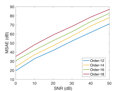
Figure 1.12: Comparison of the mean SAEs for various noise levels SNR, signal lengths, and tensor orders.

In order to separate the three signals $x_{p}(t)$ from the mixture $y(t)$, we tensorized the mixture to a $d$th-order tensor of size $2R\times 2\times\cdots\times 2\times 2R$. Under this tensorization, the exponentially decaying signals $\exp(\gamma t)$ yielded rank-1 tensors, while according to (1.282) the sinusoids have TT-representations of rank-$(2,2,\ldots,2)$. Hence, the tensors of $x(t)$ can also be represented by tensors in the TT-format of rank-$(2,2,\ldots,2)$. We were, therefore, able to approximate $\underline{\mathbf{Y}}$ as a sum of $P$ TT-tensors $\underline{\mathbf{X}}_{r}$ of rank-$(2,2,\ldots,2)$, that is, through the minimization [Phan et al., 2016]

$$\min\quad\|\underline{\mathbf{Y}}-\underline{\mathbf{X}}_{1}-\underline{\mathbf{X}}_{2}-\cdots-\underline{\mathbf{X}}_{P}\|_{F}^{2}\,.$$ (1.286)

For this purpose, a tensor $\underline{\mathbf{X}}_{p}$ in a TT-format was fitted sequentially to the residual $\underline{\mathbf{Y}}_{p}=\underline{\mathbf{Y}}-\sum_{s\neq p}\underline{\mathbf{X}}_{s}$, calculated by the difference between the data tensor $\underline{\mathbf{Y}}$ and its approximation by the other TT-tensors $\underline{\mathbf{X}}_{s}$ where $s\neq p$, that is,

$$\operatornamewithlimits{\arg\min}_{\underline{\mathbf{X}}_{p}}\|\underline{\mathbf{Y}}_{p}-\underline{\mathbf{X}}_{p}\|_{F}^{2}\,,$$ (1.287)

for $p=1,\ldots,P$. Figure 1.12 illustrates the mean SAEs (MSAE) of the estimated signals for various noise levels SNR = 0, 10, …, 50 dB, and different signal lengths $K=9\times 2^{d}$, where $d=12,14,16,18$.

On average, an improvement of 2 dB SAE is achieved if the signal is two times longer. If the signal has less than $L=9\times 2^{6}=576$ samples, the estimation quality will deteriorate by about 12 dB compared to the case when signal length of $L=9\times 2^{12}$. For such cases, we suggest to augment the signals using other tensorizations before performing the source extraction, e.g., by construction of multiway Toeplitz or Hankel tensors. Example 1.10.2 further illustrates the separation of short length signals.

1.10.2 Toeplitz Matrix and Toeplitz Tensors of Sinusoidal Signals

Toeplitz matrix of sinusoid. The Toeplitz matrix, ${\bf Y}$, of a sinusoid signal, $y(t)=\sin(\omega\,t+\phi)$, is of rank-2 and can be decomposed as

$${\bf Y}=\left[\begin{array}[]{cccc}y(1)&y(2)\\ y(2)&y(3)\\ \vdots&\vdots\\ y(I)&y(I+1)\end{array}\right]{\bf Q}_{T}\left[\begin{array}[]{cccc}y(I)&\cdots&y(L)\\ y(I-1)&\cdots&y(L-1)\\ \end{array}\right]\,,\;$$ (1.294)

where ${\bf Q}_{T}$ is invariant to the selection of folding length $I$, and has the form

$${\bf Q}_{T}=\frac{1}{\sin^{2}(\omega)}\,\left[\begin{array}[]{cc}-y(3)&y(2)\\ y(2)&-y(1)\end{array}\right]\,\,.$$ (1.297)

The above expression follows from the fact that

$$\left[\begin{array}[]{@{\hspace{.1ex}}c@{\hspace{1ex}}c@{\hspace{.1ex}}}\hskip 0.43057pt\lx@intercol\hfil y(i)\hfil\hskip 4.30554pt&y(i+1)\hfil\hskip 0.43057pt\end{array}\right]\,\left[\begin{array}[]{@{\hspace{.1ex}}c@{\hspace{1ex}}c@{\hspace{.1ex}}}\hskip 0.43057pt\lx@intercol\hfil-y(3)\hfil\hskip 4.30554pt&y(2)\hfil\hskip 0.43057pt\\ \hskip 0.43057pt\lx@intercol\hfil y(2)\hfil\hskip 4.30554pt&-y(1)\hfil\hskip 0.43057pt\end{array}\right]\,\left[\begin{array}[]{@{\hspace{1ex}}c@{\hspace{1ex}}c@{\hspace{1ex}}cc}\hskip 4.30554pt\lx@intercol\hfil y(j)\hfil\hskip 4.30554pt\\ \hskip 4.30554pt\lx@intercol\hfil y(j-1)]\hfil\hskip 4.30554pt\end{array}\right]=\sin^{2}(\omega)\,y(j-i+1)\,.$$ (1.303)

Toeplitz tensor of sinusoid. An $N$th-order Toeplitz tensor, tensorized from a sinusoidal signal, has a TT-Tucker representation

$$\underline{\mathbf{Y}}=\llbracket\underline{\mathbf{G}};{\bf U}_{1},\ldots,{\bf U}_{N-1},{\bf U}_{N}\rrbracket$$ (1.304)

where the factor matrices ${\bf U}_{n}$ are given by

$${\bf U}_{1} =\left[\begin{array}[]{@{}cc@{}}y(1)&y(2)\\ \vdots&\vdots\\ y(J_{1})&y(J_{1}+1)\end{array}\right]\,,\quad{\bf U}_{N}=\left[\begin{array}[]{@{}cc@{}}y(J_{N-1}-1)&y(J_{N-1}-2)\\ \vdots&\vdots\\ y(L)&y(L-1)\end{array}\right]\,,$$ (1.311)

$${\bf U}_{n} =\left[\begin{array}[]{@{}cc@{}}y(J_{n-1})&y(J_{n-1}+1)\\ \vdots&\vdots\\ y(J_{n}-1)&y(J_{n})\end{array}\right]\,,\quad n=2,\ldots,N-1\,,$$ (1.315)

in which $J_{n}=I_{1}+I_{2}+\cdots+I_{n}$. The core tensor $\underline{\mathbf{G}}$ is an $N$th-order tensor of size $2\times 2\times\cdots\times 2$, in a TT-format, given by

$$\underline{\mathbf{G}}=\mathopen{\hbox{\set@color${\langle}$}\kern-1.94444pt\leavevmode\hbox{\set@color${\langle}$}}\underline{\mathbf{G}}^{(1)},\underline{\mathbf{G}}^{(2)},\ldots,\underline{\mathbf{G}}^{(N-1)}\mathclose{\hbox{\set@color${\rangle}$}\kern-1.94444pt\leavevmode\hbox{\set@color${\rangle}$}},$$ (1.316)

where $\underline{\mathbf{G}}^{(1)}={\bf T}(1)$ is a matrix of size $1\times 2\times 2$, while the core tensors $\underline{\mathbf{G}}^{(n)}$, for $n=2,\ldots,N-1$, are of size $2\times 2\times 2$ and have two horizontal slices, given by

$$\underline{\mathbf{G}}^{(n)}(1,:,:) ={\bf T}(J_{n-1}-n+2)\,,\quad\underline{\mathbf{G}}^{(n)}(2,:,:)={\bf T}(J_{n-1}-n+1)\,,$$

with

$${\bf T}(I)=\frac{1}{\sin^{2}(\omega)}\,\left[\begin{array}[]{@{}cc@{}}-y(I+2)&y(I+1)\\ y(I+1)&-y(I)\end{array}\right]\,.$$ (1.319)

Following the two-stage Toeplitz tensorization, and upon applying (1.294), we can deduce the decomposition in (1.304) from that for the $(N-1)$th-order Toeplitz tensor.

Remark 5

For second-order tensorization, the core tensor $\underline{\mathbf{G}}$ in (1.316) comprises only ${\bf G}^{(1)}$, which is identical to the matrix ${\bf Q}_{T}$ in (1.297).

Quantized Toeplitz tensor. An $(L-1)$th-order Toeplitz tensor of a sinusoidal signal of length $L$ and size $2\times 2\times\cdots\times 2$ has a TT-representation with $(L-3)$ identical core tensors $\underline{\mathbf{G}}$, in the form

$$\underline{\mathbf{Y}}=\mathopen{\hbox{\set@color${\langle}$}\kern-1.94444pt\leavevmode\hbox{\set@color${\langle}$}}\underline{\mathbf{G}},\underline{\mathbf{G}},\ldots,\underline{\mathbf{G}},\left[\begin{array}[]{@{}cc@{}}y(L-1)&y(L)\\ y(L-2)&y(L-1)\end{array}\right]\mathclose{\hbox{\set@color${\rangle}$}\kern-1.94444pt\leavevmode\hbox{\set@color${\rangle}$}}\,,$$ (1.322)

where

$$\underline{\mathbf{G}}(1,:,:)=\left[\begin{array}[]{@{}cc@{}}1&0\\ 0&1\end{array}\right],\quad\underline{\mathbf{G}}(2,:,:)=\left[\begin{array}[]{@{}cc@{}}0&1\\ -1&2\cos(\omega)\end{array}\right]\,.$$ (1.327)

Example 10  Separation of short-length damped sinusoid signals.

This example illustrates the use of Toeplitz-based tensorization in the separation of damped sinusoid signals from a short-length observation. We considered a single signal composed by $P=3$ damped sinusoids of length $L=66$, given by

$$y(t) = \sum_{p=1}^{P}a_{p}\,x_{p}(t)+n(t)\,,$$ (1.328)

where

$$x(t)=\exp(\frac{-pt}{30})\,\sin(\frac{2\pi f_{p}}{f_{s}}t+\frac{p\pi}{7})\,$$ (1.329)

with frequencies $f_{p}$ = 10, 11 and 12 Hz, the sampling frequency $f_{s}$ = 300 Hz, and the mixing factors $a_{p}=p$. Additive Gaussian noise $n(t)$ was generated at a specific signal-noise-ratio.

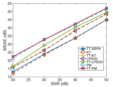
Figure 1.13: Mean SAEs (MSAE) of the estimated signals in Example 1.10.2, for various noise levels SNR.

In order to separate the three signals, $x_{p}(t)$, from the mixture $y(t)$, we first tensorized the observed signal to a 7th-order Toeplitz tensor of size $16\times 8\times 8\times 8\times 8\times 8\times 16$, then folded this tensor to a 23th-order tensor of size $2\times 2\times\cdots\times 2$. With this tensorization, according to (1.304) and (1.282), each damped sinusoid $x_{p}(t)$ had a TT-representation of rank-$(2,2,\ldots,2)$. The result produced by minimizing the cost function (1.286), annotated by TT-SEPA, is shown in Figure 1.13 as a solid line with star marker. The so obtained performance was much better than in Example 1.10.1, even for the signal length of only 66 samples.

We note that the parameters of the damped signals can be estimated using linear self-prediction (auto-regression) methods, e.g., singular value decomposition of the Hankel-type matrix as in the Kumaresan-Tufts (KT) method [Kumaresan and Tufts, 1982]. As shown in Figure 1.13, the obtained results based on the TT-decomposition were slightly better than those using the KT method. For this particular problem, the estimation performance can even be higher when applying self-prediction algorithms, which exploit the low-rank structure of damped signals, e.g., TT-KT, and TT-linear prediction methods based on SVD. For a detailed derivation of these algorithms, see [Phan et al., 2017].

1.10.3 Hankel Matrix and Hankel Tensor of Sinusoidal Signal

Hankel tensor of sinusoid. The Hankel tensor of a sinusoid signal $y(t)$ is a TT-Tucker tensor,

$$\underline{\mathbf{Y}}=\llbracket\underline{\mathbf{G}};{\bf U}_{1},{\bf U}_{2},\ldots,{\bf U}_{N}\rrbracket\,,$$ (1.330)

for which the factor matrices are defined in (1.315). The core tensor $\underline{\mathbf{G}}$ is an $N$th-order tensor of size $2\times 2\times\cdots\times 2$, in the TT-format, given by

$$\underline{\mathbf{G}}=\mathopen{\hbox{\set@color${\langle}$}\kern-1.94444pt\leavevmode\hbox{\set@color${\langle}$}}\underline{\mathbf{G}}^{(1)},\underline{\mathbf{G}}^{(2)},\ldots,\underline{\mathbf{G}}^{(N-1)}\mathclose{\hbox{\set@color${\rangle}$}\kern-1.94444pt\leavevmode\hbox{\set@color${\rangle}$}}\,,$$ (1.331)

where $\underline{\mathbf{G}}^{(1)}={\bf H}(J_{1})$ is a matrix of size $1\times 2\times 2$, while the core tensors $\underline{\mathbf{G}}^{(n)}$, for $n=2,\ldots,N-1$, are of size $2\times 2\times 2$ and have two horizontal slices, given by

$$\underline{\mathbf{G}}^{(n)}(1,:,:) ={\bf H}(J_{n}-n+1)\,,\quad\underline{\mathbf{G}}^{(n)}(2,:,:)={\bf H}(J_{n}-n+2)\,,$$

with

$${\bf H}(I)=\frac{1}{\sin^{2}(\omega)}\,\left[\begin{array}[]{@{}cc@{}}y(I)&-y(I+1)\\ -y(I-1)&y(I)\end{array}\right]\,.$$ (1.334)

Remark 6

The two TT-Tucker representations of the Toeplitz and Hankel tensors of the same sinusoid have similar factor matrices ${\bf U}_{n}$, but their core tensors are different.

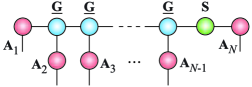
1. Folded tensor $\underline{\mathbf{G}}=\left[\left[\begin{array}[]{@{}cc@{}}1&0\\ 0&1\end{array}\right],\left[\begin{array}[]{@{}cc@{}}0&1\\ -1&0\end{array}\right]\right]$ ${\bf S}=\left[\begin{array}[]{@{}cc@{}}\sin(\phi)&\cos(\phi)\\ \cos(\phi)&-\sin(\phi)\end{array}\right]$, ${\bf A}_{n}={\bf U}_{\omega,2^{n-1}}$ 2. Toeplitz tensor $\underline{\mathbf{G}}=\left[\left[\begin{array}[]{@{}cc@{}}1&0\\ 0&1\end{array}\right],\left[\begin{array}[]{@{}c@{\hspace{1ex}}c@{}}0\hfil\hskip 4.30554pt&1\\ -1\hfil\hskip 4.30554pt&2\cos(\omega)\end{array}\right]\right]$ ${\bf A}=\left[\begin{array}[]{@{}cc@{}}y{(L-1)}&y{(L)}\\ y{(L-2)}&y{(L-1)}\end{array}\right]$ 3. Hankel tensor $\underline{\mathbf{G}}=\left[\left[\begin{array}[]{@{}c@{\hspace{1ex}}c@{}}2\cos(\omega)\hfil\hskip 4.30554pt&-1\\ 1\hfil\hskip 4.30554pt&0\end{array}\right],\left[\begin{array}[]{@{}cc@{}}1&0\\ 0&1\end{array}\right]\right]$ ${\bf A}=\left[\begin{array}[]{@{}cc@{}}y{(L-2)}&y{(L-1)}\\ y{(L-1)}&y{(L)}\end{array}\right]$

Figure 1.14: Representations of a sinusoid signal in different quantized tensor formats of size $2\times 2\times\cdots\times 2$.

Quantized Hankel tensor. An $(L-1)$th-order Hankel tensor of size $2\times 2\times\cdots\times 2$ of a sinusoid signal of length $L$ has a TT-representation with $(N-2)$ identical core tensors $\underline{\mathbf{G}}$, in the form

$$\underline{\mathbf{Y}}=\mathopen{\hbox{\set@color${\langle}$}\kern-1.94444pt\leavevmode\hbox{\set@color${\langle}$}}\underline{\mathbf{G}},\underline{\mathbf{G}},\ldots,\underline{\mathbf{G}},\left[\begin{array}[]{@{}cc@{}}y(L-2)&y(L-1)\\ y(L-1)&y(L)\end{array}\right]\mathclose{\hbox{\set@color${\rangle}$}\kern-1.94444pt\leavevmode\hbox{\set@color${\rangle}$}}\,,$$ (1.337)

where

$$\underline{\mathbf{G}}(1,:,:)=\left[\begin{array}[]{@{}cc@{}}2\cos(\omega)&-1\\ 1&0\end{array}\right]\,,\quad\underline{\mathbf{G}}(2,:,:)=\left[\begin{array}[]{@{}cc@{}}1&0\\ 0&1\end{array}\right].$$ (1.342)

Finally, representations of the sinusoid signal in various tensor format of size are summarised in Figure 1.14.

1.11 Summary

This chapter has introduced several common tensorization methods, together with their properties and illustrative applications in blind source separation, blind identification, denoising, and harmonic retrieval. The main criterion for choosing a suitable tensorization is that the tensor generated from lower-order original data must reveal the underlying low-rank tensor structure in some tensor format. For example, the folded tensors of mixtures of damped sinusoid signals have low-rank QTT representation, while the derivative tensors in blind identification admit the CP decomposition. The Toeplitz and Hankel tensor foldings augment the number of signal entries, through the replication of signal segments (redundancy), and in this way become suited to modeling of signals of short length. A property crucial to the solution via the tensor networks shown in this chapter, is that the tensors can be generated in the TT/QTT format, if the generating vector admits a low-rank QTT representation.

In modern data analytics problems, such as regression and deep learning, the number of model parameters can be huge, which renders the model intractable. Tensorization can then serve as a remedy, by representing the parameters in some low-rank tensor format. For further discussion on tensor representation of parameters in tensor regression, we refer to Chapter 2. A wide class of optimization problems including of solving linear systems, eigenvalue decomposition, singular value decomposition, Canonical Correlation Analysis (CCA) are addressed in Chapter 3. The tensor structures for Boltzmann machines and convolutional deep neural networks (CNN) are provided in Chapter 4.

Chapter 2 Supervised Learning with Tensors

Learning a statistical model that formulates a hypothesis for the data distribution merely from multiple input data samples, ${\bf x}$, without knowing the corresponding values of the response variable, $y$, is refereed to as unsupervised learning. In contrast, supervised learning methods, when seen from a probabilistic perspective, model either the joint distribution $p({\bf x},y)$ or the conditional distribution $p(y|{\bf x})$, for given training data pair $\{\mathbf{x},y\}$. Supervised learning can be categorized into regression, if $y$ is continuous, or classification, if $y$ is categorical (see also Figure 2.1).

Regression models can be categorized into linear regression and nonlinear regression. In particular, multiple linear regression is associated with multiple smaller-order predictors, while multivariate regression corresponds to a single linear regression model but with multiple predictors and multiple responses. Normally, multivariate regression tasks are encountered when the predictors are arranged as vectors, matrices or tensors of variables. A basic linear regression model in the vector form is defined as

$$y=f({\bf x};{\bf w},b)=\langle{\bf x},{\bf w}\rangle+b={\bf w}^{\text{T}}{\bf x}+b,$$ (2.1)

where ${\bf x}\in\mathbb{R}^{I}$ is the input vector of independent variables, ${\bf w}\in\mathbb{R}^{I}$ the vector of regression coefficients or weights, $b$ the bias, and $y$ the regression output or a dependent/target variable.

Such simple linear models can be applied not only for regression but also for feature selection and classification. In all the cases, those models approximate the target variable $y$ by a weighted linear combination of input variables, ${\bf w}^{\text{T}}{\bf x}+b$.

Tensor representations are often very useful in mitigating the small sample size problem in discriminative subspace selection, because the information about the structure of objects is inherent in tensors and is a natural constraint which helps reduce the number of unknown parameters in the description of a learning model. In other words, when the number of training measurements is limited, tensor-based learning machines are expected to perform better than the corresponding vector-based learning machines, as vector representations are associated with several problems, such as loss of information for structured data and over-fitting for high-dimensional data.

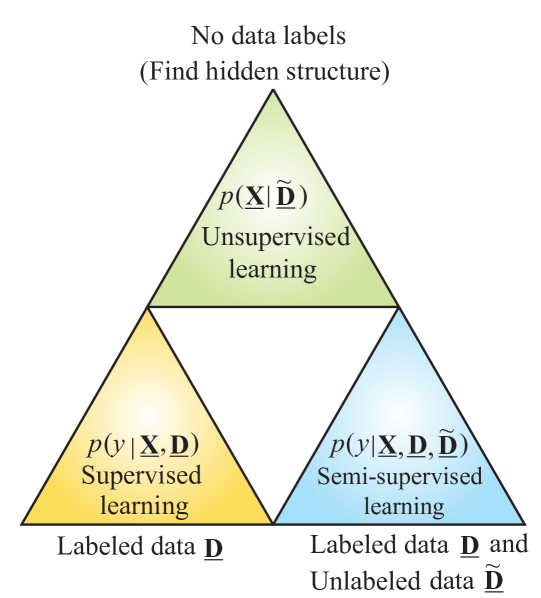
Figure 2.1: Graphical illustration of three fundamental learning approaches: Supervised, unsupervised and semi-supervised learning.

2.1 Tensor Regression

Regression is at the very core of signal processing and machine learning, whereby the output is typically estimated based on a linear combination of regression coefficients and the input regressor, which can be a vector, matrix, or tensor. In this way, regression analysis can be used to predict dependent variables (responses, outputs, estimates), from a set of independent variables (predictors, inputs, regressors), by exploring the correlations among these variables as well as explaining the inherent factors behind the observed patterns. It is also often convenient, especially regarding ill-posed cases of matrix inversion, which is inherent to regression to jointly perform regression and dimensionality reduction through, e.g., principal component regression (PCR) [Jolliffe, 1982], whereby regression is performed on a well-posed low-dimensional subspace defined through most significant principal components. With tensors being a natural generalization of vectors and matrices, tensor regression can be defined in an analogous way.

A well established and important supervised learning technique is linear or nonlinear Support Vector Regression (SVR) [Smola and Vapnik, 1997], which allows for the modeling of streaming data and is quite closely related to Support Vector Machines (SVM) [Cortes and Vapnik, 1995]. The model produced by SVR only depends on a subset of training data (support vectors), because the cost function for building the model ignores any training data that is close (within a threshold $\varepsilon$) to the model prediction.

Standard support vector regression techniques have been naturally extended to Tensor Regression (TR) or Support Tensor Machine (STM) methods [Tao et al., 2005]. In the (raw) tensor format, the TR/STM can be formulated as

$$y=f(\underline{\mathbf{X}};\underline{\mathbf{W}},b)=\langle\underline{\mathbf{X}},\underline{\mathbf{W}}\rangle+b,$$ (2.2)

where $\underline{\mathbf{X}}\in\mathbb{R}^{I_{1}\times\cdots\times I_{N}}$ is the input tensor regressor, $\underline{\mathbf{W}}\in\mathbb{R}^{I_{1}\times\cdots\times I_{N}}$ the tensor of weights (also called regression tensor or model tensor), $b$ the bias, and $y$ the regression output, $\langle\underline{\mathbf{X}},\underline{\mathbf{W}}\rangle=\operatorname{vec}\left(\underline{\mathbf{X}}\right)^{\text{T}}\operatorname{vec}\left(\underline{\mathbf{W}}\right)$ is the inner product of two tensors.

We shall denote input samples of multiple predictor variables (or features) by $\underline{{\bf X}}_{1},\ldots,\underline{{\bf X}}_{M}$ (tensors), and the actual continuous or categorical response variables by $y_{1},y_{2},\ldots,y_{M}$ (usually scalars). The training process, that is the estimation of the weight tensor $\underline{\mathbf{W}}$ and bias $b$, is carried out based on the set of available training samples $\{\underline{\mathbf{X}}_{m},y_{m}\}$ for $m=1,\ldots,M$. Upon arrival of a new training sample, the TR model is used to make predictions for that sample.

The problem is usually formulated as a minimization of the following squared cost function, given by

$$J(\underline{\mathbf{X}},y\;|\;\underline{\mathbf{W}},b)=\sum_{m=1}^{M}\Big{(}y_{m}-\big{(}\langle\underline{\mathbf{W}},\underline{\mathbf{X}}_{m}\rangle+b\big{)}\Big{)}^{2}$$ (2.3)

or the logistic loss function (usually employed in classification problems), given by

$$J(\underline{\mathbf{X}},y\;|\;\underline{\mathbf{W}},b)=\sum_{m=1}^{M}\log\left(\frac{1}{1+e^{-y_{m}(\langle\underline{\mathbf{W}},\underline{\mathbf{X}}_{m}\rangle+b)}}\right).$$ (2.4)

In practice, for very large scale problems, tensors are expressed approximately in tensor network formats, especially using Canonical Polyadic (CP), Tucker or Tensor Train (TT)/Hierarchical Tucker (HT) models [Oseledets, 2011a, Grasedyck, 2010]. In this case, a suitable representation of the weight tensor, $\underline{\mathbf{W}}$, plays a key role in the model performance. For example, the CP representation of the weight tensor, in the form

$$\underline{\mathbf{W}} = \sum_{r=1}^{R}\mathbf{u}_{r}^{(1)}\circ\mathbf{u}_{r}^{(2)}\circ\cdots\circ\mathbf{u}_{r}^{(N)}$$ (2.5)

$$= \underline{\mathbf{I}}\times_{1}\mathbf{U}^{(1)}\times_{2}\mathbf{U}^{(2)}\cdots\times_{N}\mathbf{U}^{(N)},$$

where “$\circ$” denotes the outer product of vectors, leads to a generalized linear model (GLM), called the CP tensor regression [Zhou et al., 2013].

Analogously, upon the application of Tucker multilinear rank tensor representation

$$\underline{\mathbf{W}}=\underline{\mathbf{G}}\times_{1}\mathbf{U}^{(1)}\times_{2}\mathbf{U}^{(2)}\cdots\times_{N}\mathbf{U}^{(N)},$$ (2.6)

we obtain Tucker tensor regression [Hoff, 2015, Li et al., 2013, Yu et al., 2016].

An alternative form of the multilinear Tucker regression model, proposed by Hoff [2015], assumes that the replicated observations $\{\underline{\mathbf{X}}_{m},\underline{\mathbf{Y}}_{m}\}_{m=1}^{M}$ are stacked in concatenated tensors $\underline{\mathbf{X}}\in\mathbb{R}^{I_{1}\times\cdots\times I_{N}\times M}$ and $\underline{\mathbf{Y}}\in\mathbb{R}^{J_{1}\times\cdots\times J_{N}\times M}$, which admit the following model

$$\underline{\mathbf{Y}}=\underline{\mathbf{X}}\times_{1}{\bf W}_{1}\times_{2}{\bf W}_{2}\cdots\times_{N}{\bf W}_{N}\times_{N+1}{\bf D}_{M}+\underline{\mathbf{E}},$$ (2.7)

where ${\bf D}_{M}$ is an $M\times M$ diagonal matrix, ${\bf W}_{n}\in\mathbb{R}^{J_{n}\times I_{n}}$ are the weight matrices within the Tucker model, and $\underline{\mathbf{E}}$ is a zero-mean residual tensor of the same order as $\underline{\mathbf{Y}}$. The unknown regression coefficient matrices, ${\bf W}_{n}$ can be found using the procedure outlined in Algorithm 1.

It is important to highlight that the Tucker regression model offers several benefits over the CP regression model, which include:

1. A more parsimonious modeling capability and a more compact model, especially for a limited number of available samples;

2. Ability to fully exploit multi-linear ranks, through the freedom to choose a different rank for each mode, which is essentially useful when data is skewed in dimensions (different sizes in modes);

3. Tucker decomposition explicitly models the interaction between factor matrices in different modes, thus allowing for a finer grid search over a larger modeling space.

0:  $\underline{\mathbf{X}}\in\mathbb{R}^{I_{1}\times I_{2}\times\cdots\times I_{N}\times M}$ and $\underline{\mathbf{Y}}\in\mathbb{R}^{J_{1}\times I_{2}\times\cdots\times J_{N}\times M}$. 0:  $\{\mathbf{W}_{n}\},n=1,\ldots,N$. 1:  Initialize randomly ${\bf W}_{n}$ for $n=1,\ldots,N$. 2:  while not converged or iteration limit is not reached do 3:     for $n=1$ to $N$ do 4:        $\underline{{\bf X}}^{(n)}=\underline{{\bf X}}\times_{1}{\bf W}_{1}\cdots\times_{n-1}{\bf W}_{n-1}\times_{n+1}{\bf W}_{n+1}\cdots\times_{N}{\bf W}_{N}$ 5:        Matricize tensors $\underline{{\bf X}}^{(n)}$ and $\underline{{\bf Y}}$ into their respective unfolded matrices ${\bf X}^{(n)}_{(n)}$ and ${\bf Y}_{(n)}$ 6:        Compute ${\bf W}_{n}={\bf Y}_{(n)}({\bf X}_{(n)}^{(n)})^{\text{T}}\left({\bf X}_{(n)}^{(n)}\;({\bf X}_{(n)}^{(n)})^{\text{T}}\right)^{-1}$ 7:     end for 8:  end while

Algorithm 1 Multilinear Tucker Regression

Both the CP and Tucker tensor regression models can be solved by alternating least squares (ALS) algorithms which sequentially estimate one factor matrix at a time while keeping other factor matrices fixed. To deal with the curse of dimensionality, various tensor network decompositions can be applied, such as the TT/HT decomposition for very high-order tensors [Oseledets, 2011a, Grasedyck, 2010]. When the weight tensor $\underline{\mathbf{W}}$ in (2.2) is represented by a low-rank HT decomposition, this is referred to as the H-Tucker tensor regression [Hou, 2017].

Remark 1. In some applications, the weight tensor, $\underline{{\bf W}}$, is of a higher-order than input tensors, $\underline{{\bf X}}_{m}$, this yields a more general tensor regression model

$$\underline{\mathbf{Y}}_{m}=\langle\underline{\mathbf{X}}_{m}|\underline{\mathbf{W}}\rangle+\underline{\mathbf{E}}_{m},\qquad m=1,\ldots,M,$$ (2.8)

where $\langle\underline{\mathbf{X}}_{m}|\underline{\mathbf{W}}\rangle$ denotes a tensor contraction along the first $N$ modes of an $N$th-order input (covariate) tensor, $\underline{\mathbf{X}}_{m}\in\mathbb{R}^{I_{1}\times\cdots\times I_{N}}$, and a $P$th-order weight tensor, $\underline{\mathbf{W}}\in\mathbb{R}^{I_{1}\times\cdots\times I_{P}}$, with $P>N$, while $\underline{\mathbf{E}}\in\mathbb{R}^{I_{P+1}\times\cdots\times I_{P}}$ is the residual tensor and $\underline{\mathbf{Y}}\in\mathbb{R}^{I_{P+1}\times\cdots\times I_{P}}$ the response tensor.

Observe that the tensor inner product is equivalent to a contraction of two tensors of the same order (which is a scalar) while a contraction of two tensors of different orders, $\underline{\mathbf{X}}\in\mathbb{R}^{I_{1}\times\cdots\times I_{N}}$ and $\underline{\mathbf{W}}\in\mathbb{R}^{I_{1}\times\cdots\times I_{P}}$, with $P>N$, is defined as a tensor $\underline{{\bf Y}}\in\mathbb{R}^{I_{N+1}\times\cdots\times I_{P}}$ of $(P-N)$th-order with entries

$$\langle\underline{\mathbf{X}}|\underline{\mathbf{W}}\rangle_{i_{N+1},\ldots,i_{P}}=\sum_{i_{1}=1}^{I_{1}}\cdots\sum_{i_{N}=1}^{I_{N}}x_{i_{1},\ldots,i_{N}}\;w_{i_{1},\ldots,i_{N},i_{N+1},\ldots,i_{P}}.$$ (2.9)

Many regression problems are special cases of the general tensor regression model in (2.8), including the multi-response regression, vector autoregressive model and pair-wise interaction tensor model (see [Raskutti and Yuan, 2015] and references therein).

In summary, the aim of tensor regression is to estimate the entries of a weight tensor, $\underline{\mathbf{W}}$, based on available input-output observations $\{\underline{\mathbf{X}}_{m},\underline{\mathbf{Y}}_{m}\}$. In a more general scenario, support tensor regression (STR) aims to identify a nonlinear function, $f:\mathbb{R}^{I_{1}\times I_{2}\times\cdots\times I_{N}}\rightarrow\mathbb{R}$, from a collection of observed input-output data pairs $\{\underline{\mathbf{X}}_{m},y_{m}\}_{m=1}^{M}$ generated from the model

$$y_{m}=f(\underline{\mathbf{X}}_{m})+\varepsilon,$$ (2.10)

where the input $\underline{\mathbf{X}}_{m}$ has a tensor structure, the output $y_{m}$ is a scalar, and $\varepsilon$ is also a scalar which represents the error.

Unlike linear regression models, nonlinear regression models have the ability to characterize complex nonlinear dependencies in data, in which the responses are modeled through a combination of nonlinear parameters and predictors, with the nonlinear parameters usually taking the form of an exponential function, trigonometric function, power function, etc. The nonparametric counterparts, so called nonparametric regression models, frequently appear in machine learning, such as Gaussian Processes (GP) (see [Zhao et al., 2013b, Hou, 2017] and references therein).

2.2 Regularized Tensor Models

Regularized tensor models aims to reduce the complexity of tensor regression models through constraints (restrictions) on the model parameters, $\underline{{\bf W}}$. This is particularly advantageous for problems with a large number of features but a small number of data samples.

Regularized linear tensor models can be generally formulated as

$$\min_{\underline{{\bf W}},b}\,f(\underline{{\bf X}},y)=J(\underline{{\bf X}},y\;|\;\underline{{\bf W}},b)+\lambda R(\underline{{\bf W}}),$$ (2.11)

where $J(\underline{{\bf X}},y\;|\;\underline{{\bf W}},b)$ denotes a loss (error) function, $R(\underline{{\bf W}})$ is a regularization term, while the parameter $\lambda>0$ controls the trade-off between the contributions of the original loss function and regularization term.

One such well-known regularized linear model is the Frobenius-norm regularized model for support vector regression, called Grouped LASSO [Tibshirani, 1996a], which employs logistic loss and $\ell_{1}$-norm regularization for simultaneous classification (or regression) and feature selection. Another very popular model of this kind is the support vector machines (SVM) [Cortes and Vapnik, 1995] which uses a hinge loss in the form $l(\hat{y})=\text{max}(0,1-y\hat{y})$, where $\hat{y}$ is the prediction and $y$ the true label.

In regularized tensor regression, when the regularization is performed via the Frobenius norm, $\|\underline{{\bf W}}\|^{2}_{F}=\langle\underline{{\bf W}},\underline{{\bf W}}\rangle$, we arrive at the standard Tikhonov regularization, while using the $\ell_{1}$ norm, $\|\cdot\|_{\ell_{1}}$, we impose classical sparsity constraints. The advantage of tensors over vectors and matrices is that we can exploit the flexibility in the choice of sparsity profiles. For example, instead of imposing global sparsity for the whole tensor, we can impose sparsity for slices or fibers if there is a need to enforce some fibers or slices to have most of their entries zero. In such a case, similarly to group LASSO, we can apply group-based $\ell_{1}$-norm regularizers, such as the $\ell_{2,1}$ norm, i.e., $\|\mathbf{X}\|_{2,1}=\sum_{j=1}^{J}\|\mathbf{x}_{j}\|_{2}$.

Similarly to matrices, the various rank properties can also be employed for tensors, and are much richer and more complex due to the multidimensional structure of tensors. In addition to sparsity constraints, a low-rank of a tensor can be exploited as a regularizer, such as the canonical rank or multilinear (Tucker) rank, together with various more sophisticated tensor norms like the nuclear norm or latent norm of the weight tensor $\underline{{\bf W}}$.

The low-rank regularization problem can be formulated as

$$\begin{split}\min_{\underline{\mathbf{W}}}\;J(\underline{\mathbf{X}},y\;|\;\underline{\mathbf{W}},b),\quad\mbox{s.t.}\quad\text{multilinear rank}(\underline{\mathbf{W}})\leq R.\end{split}$$ (2.12)

Such a formulation allows us to estimate a weight tensor, $\underline{\mathbf{W}}\in\mathbb{R}^{I_{1}\times\cdots\times I_{N}}$, that minimizes the empirical loss $J$, subject to the constraint that the multilinear rank of $\underline{\mathbf{W}}$ is at most $R$. Equivalently, this implies that the weight tensor, $\underline{\mathbf{W}}$, admits a low-dimensional factorization in the form $\underline{\mathbf{W}}=\underline{\mathbf{G}}\times_{1}\mathbf{U}^{(1)}\times_{2}\mathbf{U}^{(2)}\cdots\times_{N}\mathbf{U}^{(N)}$.

Low rank structure of tensor data has been successfully utilized in applications including missing data imputation [Liu et al., 2013, Zhao et al., 2015], multilinear robust principal component analysis [Inoue et al., 2009], and subspace clustering [Zhang et al., 2015a]. Instead of low-rank properties of data itself, low-rank regularization can be also applied to learning coefficients in regression and classification [Yu et al., 2016].

Similarly, for very large-scale problems, we can also apply the tensor train (TT) decomposition as the constraint, to yield

$$\begin{split}\min_{\underline{\mathbf{W}}}\,J(\underline{{\bf X}},y\;|\;\underline{{\bf W}},b),\quad\mbox{s.t.}\quad\underline{\mathbf{W}}=\mathopen{\hbox{\set@color${\langle}$}\kern-1.94444pt\leavevmode\hbox{\set@color${\langle}$}}\underline{\mathbf{G}}^{(1)},\ldots,\underline{\mathbf{G}}^{(N)}\mathclose{\hbox{\set@color${\rangle}$}\kern-1.94444pt\leavevmode\hbox{\set@color${\rangle}$}}.\end{split}$$ (2.13)

In this way, the weight tensor $\underline{\mathbf{W}}$ is approximated by a low-TT rank tensor of the TT-rank $(R_{1},\ldots,R_{N-1})$ of at most $R$.

The low-rank constraint for the tensor $\underline{\mathbf{W}}$ can also be formulated through the tensor norm, in the form [Wimalawarne et al., 2016]

$$\min_{\underline{\mathbf{W}},b}\,(J(\underline{{\bf X}},y\;|\;\underline{{\bf W}},b)+\lambda\|\underline{\mathbf{W}}\|),$$ (2.14)

where $\|\cdot\|$ is a suitably chosen tensor/matrix norm.

One of the important and useful tensor norms is the tensor nuclear norm [Liu et al., 2013] or the (overlapped) trace norm [Wimalawarne et al., 2014], which can be defined for a tensor $\underline{\mathbf{W}}\in\mathbb{R}^{I_{1}\times\cdots\times I_{N}}$ as

$$\|\underline{\mathbf{W}}\|_{*}=\sum_{n=1}^{N}\|\mathbf{W}_{(n)}\|_{*},$$ (2.15)

where $\|\mathbf{W}_{(n)}\|_{*}=\sum_{i}\sigma_{i}$, $\sigma_{i}$ denotes the $i$th singular value of $\mathbf{W}_{(n)}$. The overlapped tensor trace norm can be viewed as a direct extension of the matrix trace norm, since it uses unfolding matrices of a tensor in all of its modes, and then computes the sums of trace norms of those unfolding matrices. Regularization based on the overlapped trace norm can also be viewed as an overlapped group regularization, due to the fact that the same tensor is unfolded over all modes and regularized using the trace norm.

Recently Tomioka and Suzuki [2013] proposed the latent trace norm of a tensor, which takes a mixture of $N$ latent tensors, $\underline{\mathbf{W}}^{(n)}$, and regularizes each of them separately, as in (2.15), to give

$$\|\underline{\mathbf{W}}\|_{latent}=\inf_{\underline{\mathbf{W}}}\;\sum_{n=1}^{N}\|\mathbf{W}_{(n)}^{(n)}\|_{*},$$ (2.16)

where $\underline{\mathbf{W}}=\underline{\mathbf{W}}^{(1)}+\underline{\mathbf{W}}^{(2)}+\cdots+\underline{\mathbf{W}}^{(N)}$ and $\mathbf{W}^{(n)}_{(n)}$ denotes the unfolding of $\underline{\mathbf{W}}^{(n)}$ in its $n$th mode. In contrast to the nuclear norm, the latent tensor trace norm effectively regularizes different latent tensors in each unfolded mode, which makes it possible for the latent tensor trace norm to identify (in some cases) a latent tensor with the lowest possible rank. In general, the content of each latent tensor depends on the rank of its unfolding matrices.

Remark 2. A major drawback of the latent trace norm approach is its inability to identify the rank of a tensor, when the rank value is relatively close to its dimension (size). In other words, if a tensor has a mode with a dimension (size) much smaller than other modes, the latent trace norm may be incorrectly estimated. To deal with this problem, the scaled latent norm was proposed by Wimalawarne et al. [2014] which is defined as

$$\|\underline{\mathbf{W}}\|_{scaled}=\inf_{\underline{\mathbf{W}}}\;\sum_{n=1}^{N}\frac{1}{\sqrt{I_{n}}}\|\mathbf{W}^{(n)}_{(n)}\|_{*},$$ (2.17)

where $\underline{\mathbf{W}}=\underline{\mathbf{W}}^{(1)}+\underline{\mathbf{W}}^{(2)}+\cdots+\underline{\mathbf{W}}^{(N)}$. Owing to the normalization by the mode size, in the form of (2.17), the scaled latent trace norm scales with mode dimension, and thus estimates more reliably the rank, even when the sizes of various modes are quite different.

The state-of-the-art tensor regression models therefore employ the scaled latent trace norm, and are solved by the following optimization problem

$$P(\underline{\mathbf{W}},b)=\min_{\underline{\mathbf{W}},b}\,\bigg{(}\sum_{m=1}^{M}\Big{(}y_{m}-\big{(}\langle\underline{\mathbf{W}},\underline{\mathbf{X}}_{m}\rangle+b\big{)}\Big{)}^{2}+\sum_{n=1}^{N}\lambda_{n}\|\mathbf{W}^{(n)}_{(n)}\|_{*}\bigg{)},$$ (2.18)

where $\underline{\mathbf{W}}=\underline{\mathbf{W}}^{(1)}+\underline{\mathbf{W}}^{(2)}+\cdots+\underline{\mathbf{W}}^{(N)}$, for $n=1,\ldots,N$, and for any given regularization parameter $\lambda$, where $\lambda_{n}=\lambda$ in the case of latent trace norm and $\lambda_{n}=\frac{\lambda}{\sqrt{I_{n}}}$ in the case of the scaled latent trace norm, while $\mathbf{W}^{(n)}_{(n)}$ denotes the unfolding of $\underline{\mathbf{W}}^{(n)}$ in its $n$th mode.

Remark 3. Note that the above optimization problems involving the latent and scaled latent trace norms require a large number ($N\prod_{n}I_{n}$) of variables in $N$ latent tensors.

Moreover, the existing methods based on SVD are infeasible for very large-scale applications. Therefore, for very large scale high-order tensors, we need to use tensor network decompositions and perform all operations in tensor networks formats, taking advantage of their lower-order core tensors.

2.3 Higher-Order Low-Rank Regression (HOLRR)

Consider a full multivariate regression task in which the response has a tensor structure. Let $f:\mathbb{R}^{I_{0}}\rightarrow\mathbb{R}^{I_{1}\times I_{2}\times\cdots\times I_{N}}$ be a function we desire to learn from input-output data, $\{\mathbf{x}_{m},\underline{\mathbf{Y}}_{m}\}_{m=1}^{M}$, drawn from the model $\underline{\mathbf{Y}}=\underline{\mathbf{W}}\;\bar{\times}_{1}\;\mathbf{x}+\underline{\mathbf{E}}$, where $\underline{\mathbf{E}}$ is an error tensor, ${\bf x}\in\mathbb{R}^{I_{0}}$, $\underline{{\bf Y}}\in\mathbb{R}^{I_{1}\times\cdots\times I_{N}}$, and $\underline{\mathbf{W}}\in\mathbb{R}^{I_{0}\times I_{1}\times\cdots\times I_{N}}$ is a tensor of regression coefficients. The extension of low-rank regression methods to tensor-structured responses can be achieved by enforcing low multilinear rank of the regression tensor, $\underline{\mathbf{W}}$, to yield the so-called higher-order low rank regression (HOLRR) [Rabusseau and Kadri, 2016, Sun and Li, 2016]. The aim is to find a low-rank regression tensor, $\underline{\mathbf{W}}$, which minimizes the loss function based on the training data.

To avoid numerical instabilities and to prevent overfitting, it is convenient to employ a ridge regularization of the objective function, leading to the following minimization problem

$$\begin{split}\min_{\underline{\mathbf{W}}}&\sum_{m=1}^{M}\|\underline{\mathbf{W}}\;\bar{\times}_{1}\;\mathbf{x}_{m}-\underline{\mathbf{Y}}_{m}\|_{F}^{2}+\gamma\|\underline{\mathbf{W}}\|_{F}^{2}\\ \mbox{s.t.}\quad&\mbox{multilinear rank}(\underline{\mathbf{W}})\leq(R_{0},R_{1},\ldots,R_{N}),\end{split}$$ (2.19)

for some given integers $R_{0},R_{1},\ldots,R_{N}$.

Taking into account the fact that input vectors, ${\bf x}_{m}$, can be concatenated into an input matrix, ${\bf X}=[{\bf x}_{1},\ldots,{\bf x}_{M}]^{\text{T}}\in\mathbb{R}^{M\times I_{0}}$, the above optimization problem can be reformulated in the following form

$$\begin{split}&\min_{\underline{\mathbf{W}}}\,\|\underline{\mathbf{W}}\times_{1}\mathbf{X}-\underline{\mathbf{Y}}\|_{F}^{2}+\gamma\|\underline{\mathbf{W}}\|_{F}^{2}\\ \mbox{s.t.}\quad&\underline{\mathbf{W}}=\underline{\mathbf{G}}\times_{1}\mathbf{U}^{(0)}\times_{2}\mathbf{U}^{(1)}\cdots\times_{N+1}\mathbf{U}^{(N)},\\ &\mathbf{U}^{(n)\,\text{T}}\mathbf{U}^{(n)}=\mathbf{I}\quad\text{for}\quad n=1,\ldots,N,\end{split}$$ (2.20)

where the output tensor $\underline{\mathbf{Y}}$ is obtained by stacking the output tensors $\underline{\mathbf{Y}}_{m}$ along the first mode $\underline{\mathbf{Y}}(m,:,\ldots,:)=\underline{\mathbf{Y}}_{m}$. The regression function can be rewritten as

$$f:\mathbf{x}\mapsto\underline{\mathbf{G}}\times_{1}\mathbf{x}^{\text{T}}\mathbf{U}^{(0)}\times_{2}\mathbf{U}^{(1)}\cdots\times_{N+1}\mathbf{U}^{(N)}.$$ (2.21)

This minimization problem can be reduced to finding ($N+1$) projection matrices onto subspaces of dimensions, $R_{0},R_{1},\ldots,R_{N}$, where the core tensor $\underline{\mathbf{G}}$ is given by

$$\underline{\mathbf{G}}={\underline{\mathbf{Y}}}\times_{1}(\mathbf{U}^{(0)\,\text{T}}({\mathbf{X}}^{\text{T}}{\mathbf{X}}+\gamma\mathbf{I})\mathbf{U}^{(0)})^{-1}\mathbf{U}^{(0)\,\text{T}}{\mathbf{X}}^{\text{T}}\times_{2}\mathbf{U}^{(1)\,\text{T}}\cdots\times_{N+1}\mathbf{U}^{(N)\,\text{T}},$$ (2.22)

and the orthogonal matrices $\mathbf{U}^{(n)}$   for $n=0,1,\ldots,N$ can be computed by the eigenvectors of

$$\Bigg{\{}\begin{array}[]{ll}(\mathbf{X}^{\text{T}}\mathbf{X}+\gamma\mathbf{I})^{-1}\mathbf{X}^{\text{T}}\mathbf{Y}_{(1)}\mathbf{Y}_{(1)}^{\text{T}}\mathbf{X},&\quad n=0,\\ \mathbf{Y}_{(n)}\mathbf{Y}_{(n)}^{\text{T}},&otherwise.\end{array}$$ (2.23)

In other words, by the computation of $R_{n}$ largest eigenvalues and the corresponding eigenvectors. The HOLRR procedure is outlined in Algorithm 2.

0:  $\mathbf{X}\in\mathbb{R}^{M\times I_{0}}$, $\underline{\mathbf{Y}}\in\mathbb{R}^{M\times I_{1}\times\cdots\times I_{N}}$, rank $(R_{0},R_{1},\ldots,R_{N})$ and a regularization parameter $\gamma$. 0:  $\underline{\mathbf{W}}=\underline{\mathbf{G}}\times_{1}\mathbf{U}^{(0)}\times_{2}\mathbf{U}^{(1)}\cdots\times_{N+1}\mathbf{U}^{(N)}$ 1:  $\mathbf{U}^{(0)}\leftarrow$ top $R_{0}$ eigenvectors of $(\mathbf{X}^{\text{T}}\mathbf{X}+\gamma\mathbf{I})^{-1}\mathbf{X}^{\text{T}}\mathbf{Y}_{(1)}\mathbf{Y}_{(1)}^{\text{T}}\mathbf{X}$ 2:  for $n=1$ to $N$ do 3:     $\mathbf{U}^{(n)}\leftarrow$ top $R_{n}$ eigenvectors of $\mathbf{Y}_{(n)}\mathbf{Y}_{(n)}^{\text{T}}$ 4:  end for 5:  $\mathbf{T}=\left(\mathbf{U}^{(0)\,\text{T}}({\mathbf{X}}^{\text{T}}{\mathbf{X}}+\gamma\mathbf{I})\mathbf{U}^{(0)}\right)^{-1}\mathbf{U}^{(0)\,\text{T}}{\mathbf{X}}^{\text{T}}$ 6:  $\underline{\mathbf{G}}\leftarrow{\underline{\mathbf{Y}}}\times_{1}\mathbf{T}\times_{2}\mathbf{U}^{(1)\,\text{T}}\cdots\times_{N+1}\mathbf{U}^{(N)\,\text{T}}$

Algorithm 2 Higher-Order Low-Rank Regression (HOLRR)

2.4 Kernelized HOLRR

The HOLRR can be extended to its kernelized version, the kernelized HOLRR (KHOLRR). Let $\phi:\mathbb{R}^{I_{0}}\rightarrow\mathbb{R}^{L}$ be a feature map and let $\mbox{\boldmath$\Phi$}\in\mathbb{R}^{M\times L}$ be a matrix with row vectors $\phi(\mathbf{x}_{m}^{\text{T}})$ for $m\in\{1,\ldots,M\}$. The HOLRR problem in the feature space boils down to the ridge regularized minimization problem

$$\begin{split}&\min_{\underline{\mathbf{W}}}\,\|\underline{\mathbf{W}}\times_{1}\mbox{\boldmath$\Phi$}-\underline{\mathbf{Y}}\|_{F}^{2}+\gamma\|\underline{\mathbf{W}}\|_{F}^{2}\\ \mbox{s.t.}\quad&\underline{\mathbf{W}}=\underline{\mathbf{G}}\times_{1}\mathbf{U}^{(0)}\times_{2}\mathbf{U}^{(1)}\cdots\times_{N+1}\mathbf{U}^{(N)},\\ &\text{and}\quad\mathbf{U}^{(n)\,\text{T}}\mathbf{U}^{(n)}=\mathbf{I}\quad\text{for}\quad n=0,\ldots,N.\end{split}$$ (2.24)

The tensor $\underline{\mathbf{W}}$ is represented in a Tucker format. Then, the core tensor $\underline{\mathbf{G}}$ is given by

$$\underline{\mathbf{G}}={\underline{\mathbf{Y}}}\times_{1}(\mathbf{U}^{(0)\,\text{T}}{\mathbf{K}}({\mathbf{K}}+\gamma\mathbf{I})\mathbf{U}^{(0)})^{-1}\mathbf{U}^{(0)\,\text{T}}{\mathbf{K}}\times_{2}\mathbf{U}^{(1)\,\text{T}}\cdots\times_{N+1}\mathbf{U}^{(N)\,\text{T}},$$ (2.25)

where $\mathbf{K}$ is the kernel matrix and the orthogonal matrices $\mathbf{U}^{(n)},n=0,1,\ldots,N$, can be computed via the eigenvectors of

$$\Bigg{\{}\begin{array}[]{ll}(\mathbf{K}+\gamma\mathbf{I})^{-1}\mathbf{Y}_{(1)}\mathbf{Y}_{(1)}^{\text{T}}\mathbf{K},&\quad n=0,\\ \mathbf{Y}_{(n)}\mathbf{Y}_{(n)}^{\text{T}},&otherwise,\end{array}$$ (2.26)

which corresponds to the computation of $R_{n}$ largest eigenvalues and the associated eigenvectors, where $\mathbf{K}=\mbox{\boldmath$\Phi$}\mbox{\boldmath$\Phi$}^{\text{T}}$ is the kernel matrix. The KHOLRR procedure is outlined in Algorithm 3.

0:  Gram matrix $\mathbf{K}\in\mathbb{R}^{M\times M}$, $\underline{\mathbf{Y}}\in\mathbb{R}^{M\times I_{1}\times\cdots\times I_{N}}$, rank $(R_{0},R_{1},\ldots,R_{N})$ and a regularization parameter $\gamma$. 0:  $\underline{\mathbf{W}}=\underline{\mathbf{G}}\times_{1}\mathbf{U}^{(0)}\times_{2}\mathbf{U}^{(1)}\cdots\times_{N+1}\mathbf{U}^{(N)}$ 1:  $\mathbf{U}^{(0)}\leftarrow$ top $R_{0}$ eigenvectors of $(\mathbf{K}+\gamma\mathbf{I})^{-1}\mathbf{Y}_{(1)}\mathbf{Y}_{(1)}^{\text{T}}\mathbf{K}$ 2:  for $n=1$ to $N$ do 3:     $\mathbf{U}^{(n)}\leftarrow$ top $R_{n}$ eigenvectors of $\mathbf{Y}_{(n)}\mathbf{Y}_{(n)}^{\text{T}}$ 4:  end for 5:  $\mathbf{T}=\left(\mathbf{U}^{(0)\,\text{T}}{\mathbf{K}}({\mathbf{K}}+\gamma\mathbf{I})\mathbf{U}^{(0)}\right)^{-1}\mathbf{U}^{(0)\,\text{T}}{\mathbf{K}}$ 6:  $\underline{\mathbf{G}}\leftarrow{\underline{\mathbf{Y}}}\times_{1}\mathbf{T}\times_{2}\mathbf{U}^{(1)\,\text{T}}\cdots\times_{N+1}\mathbf{U}^{(N)\,\text{T}}$

Algorithm 3 Kernelized Higher-Order Low-Rank Regression (KHOLRR)

Note that the kernel HOLRR returns the weight tensor, $\underline{\mathbf{W}}\in\mathbb{R}^{M\times I_{1}\times\cdots\times I_{N}}$, which is used to define the regression function

$$f:\mathbf{x}\mapsto\underline{\mathbf{W}}\bar{\times}_{1}\mathbf{k}_{x}=\sum_{m=1}^{M}k(\mathbf{x},\mathbf{x}_{m})\underline{\mathbf{W}}_{m},$$ (2.27)

where $\underline{\mathbf{W}}_{m}=\underline{\mathbf{W}}(m,:,\ldots,:)\in\mathbb{R}^{I_{1}\times\cdots\times I_{N}}$ and the $m$th component of $\mathbf{k}_{x}$ is $k(\mathbf{x},\mathbf{x}_{m})$.

2.5 Higher-Order Partial Least Squares (HOPLS)

In this section, Partial Least Squares (PLS) method is briefly presented followed by its generalizations to tensors.

2.5.1 Standard Partial Least Squares

The principle behind the PLS method is to search for a common set of latent vectors in the independent variable $\mathbf{X}\in\mathbb{R}^{I\times J}$ and the dependent variable $\mathbf{Y}\in\mathbb{R}^{I\times M}$ by performing their simultaneous decomposition, with the constraint that the components obtained through such a decomposition explain as much as possible of the covariance between $\mathbf{X}$ and $\mathbf{Y}$. This problem can be formulated as (see also Figure 2.2)

$$\mathbf{X} = \mathbf{T}\mathbf{P}^{\text{T}}+\mathbf{E}=\sum_{r=1}^{R}{\mathbf{t}_{r}\mathbf{p}_{r}^{\text{T}}}+\mathbf{E},$$ (2.28)

$$\mathbf{Y} = \mathbf{T}\mathbf{D}\mathbf{C}^{\text{T}}+\mathbf{F}=\sum_{r=1}^{R}d_{rr}{\mathbf{t}_{r}\mathbf{c}_{r}^{\text{T}}}+\mathbf{F},$$ (2.29)

where $\mathbf{T}=[\mathbf{t}_{1},\mathbf{t}_{2},\ldots,\mathbf{t}_{R}]\in\mathbb{R}^{I\times R}$ consists of $R$ orthonormal latent variables from $\mathbf{X}$, and a matrix $\mathbf{U}=\mathbf{T}\mathbf{D}=[\mathbf{u}_{1},\mathbf{u}_{2},\ldots,\mathbf{u}_{R}]\in\mathbb{R}^{I\times R}$ represents latent variables from $\mathbf{Y}$ which have maximum covariance with the latent variables, ${\bf T}$, in $\mathbf{X}$. The matrices $\mathbf{P}$ and $\mathbf{C}$ represent loadings (PLS regression coefficients), and $\mathbf{E},\mathbf{F}$ are respectively the residuals for $\mathbf{X}$ and $\mathbf{Y}$, while $\mathbf{D}$ is a scaling diagonal matrix.

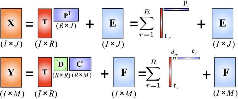
Figure 2.2: The standard PLS model which performs data decomposition as a sum of rank-one matrices.

The PLS procedure is recursive, so that in order to obtain the set of first latent components in $\mathbf{T}$, the standard PLS algorithm finds the two sets of weight vectors, $\mathbf{w}$ and $\mathbf{c}$, through the following optimization problem

$$\max_{\{\mathbf{w},\mathbf{c}\}}\;\left(\mathbf{w}^{\text{T}}\mathbf{X}^{\text{T}}\mathbf{Y}\mathbf{c}\right)^{2},\quad\mbox{s.t. }\quad\mathbf{w}^{\text{T}}\mathbf{w}=1,\quad\mathbf{c}^{\text{T}}\mathbf{c}=1.$$ (2.30)

The obtained latent variables are given by $\mathbf{t}={\mathbf{X}\mathbf{w}}/{\|\mathbf{X}\mathbf{w}\|_{2}^{2}}$ and $\mathbf{u}=\mathbf{Yc}$. In doing so, we have made the following two assumptions: i) the latent variables $\{\mathbf{t}_{r}\}_{r=1}^{R}$ are good predictors of $\mathbf{Y}$; ii) the linear (inner) relation between the latent variables $\mathbf{t}$ and $\mathbf{u}$ does exist, that is $\mathbf{U}=\mathbf{TD}+\mathbf{Z}$, where $\mathbf{Z}$ denotes the matrix of Gaussian i.i.d. residuals. Upon combining with the decomposition of $\mathbf{Y}$, in (2.29), we have

$$\mathbf{Y}=\mathbf{TDC}^{\text{T}}+(\mathbf{ZC}^{\text{T}}+\mathbf{F})=\mathbf{T}\mathbf{D}\mathbf{C}^{\text{T}}+\mathbf{F}^{*},$$ (2.31)

where $\mathbf{F}^{*}$ is the residual matrix. Observe from (2.31) that the problem boils down to finding common latent variables, $\mathbf{T}$, that best explain the variance in both $\mathbf{X}$ and $\mathbf{Y}$. The prediction of new dataset $\mathbf{X}^{*}$ can then be performed by $\mathbf{Y}^{*}\approx\mathbf{X}^{*}\mathbf{W}\mathbf{D}\mathbf{C}^{\text{T}}$.

2.5.2 The $N$-way PLS Method

The multi-way PLS (called $N$-way PLS) proposed by Bro [1996] is a simple extension of the standard PLS. The method factorizes an $N$th-order tensor, $\underline{\mathbf{X}}$, based on the CP decomposition, to predict response variables represented by $\mathbf{Y}$, as shown in Figure 2.3. For a 3rd-order tensor, $\underline{\mathbf{X}}\in\mathbb{R}^{I\times J\times K}$, and a multivariate response matrix, $\mathbf{Y}\in\mathbb{R}^{I\times M}$, with the respective elements $x_{ijk}$ and $y_{im}$, the tensor of independent variables, $\underline{\mathbf{X}}$, is decomposed into one latent vector $\mathbf{t}\in\mathbb{R}^{I\times 1}$ and two loading vectors, $\mathbf{p}\in\mathbb{R}^{J\times 1}$ and $\mathbf{q}\in\mathbb{R}^{K\times 1}$, i.e., one loading vector per mode. As shown in Figure 2.3, the $3$-way PLS (the $N$-way PLS for $N=3$) performs the following simultaneous tensor and matrix decompositions

$$\underline{\mathbf{X}}=\sum_{r=1}^{R}\mathbf{t}_{r}\circ\mathbf{p}_{r}\circ\mathbf{q}_{r}+\underline{\mathbf{E}},\qquad\mathbf{Y}=\sum_{r=1}^{R}d_{rr}\,\mathbf{t}_{r}\mathbf{c}_{r}^{\text{T}}+\mathbf{F}.$$ (2.32)

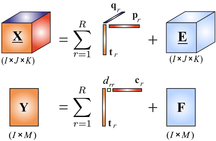
Figure 2.3: The $N$-way PLS model performs a joint decomposition of data tensors/matrices as a sum of rank-one tensors through standard CP decomposition for the independent variables, $\underline{\mathbf{X}}$, and a sum of rank-one matrices for the responses, $\mathbf{Y}$.

The objective is to find the vectors $\mathbf{p}_{r},\mathbf{q}_{r}$ and $\mathbf{c}_{r}$, which are the solutions of the following optimization problem

$$\{\mathbf{p}_{r},\mathbf{q}_{r},\mathbf{c}_{r}\} = \arg\max_{\mathbf{p}_{r},\mathbf{q}_{r},\mathbf{c}_{r}}\ \mbox{cov}(\mathbf{t}_{r},\mathbf{u}_{r}),$$

$$\mbox{s.t.}\quad\mathbf{t}_{r}=\underline{\mathbf{X}}\bar{\times}_{1}\mathbf{p}_{r}\bar{\times}_{2}\mathbf{q}_{r},\qquad\mathbf{u}_{r} = \mathbf{Yc}_{r},\quad\|\mathbf{p}_{r}\|^{2}_{2}=\|\mathbf{q}_{r}\|^{2}_{2}=\|\mathbf{c}_{r}\|^{2}_{2}=1.$$

Again, the problem boils down to finding the common latent variables, $\mathbf{t}_{r}$, in both $\underline{\mathbf{X}}$ and $\underline{\mathbf{Y}}$, that best explain the variance in $\underline{\mathbf{X}}$ and $\underline{\mathbf{Y}}$. The prediction of a new dataset, $\underline{\mathbf{X}}^{*}$, can then be performed by $\mathbf{Y}^{*}_{(1)}\approx\mathbf{X}_{(1)}^{*}(\mathbf{Q}\bigodot\mathbf{P})^{-1}\mathbf{D}\mathbf{C}^{\text{T}}$, where $\mathbf{P}=[\mathbf{p}_{1},\ldots,\mathbf{p}_{R}]$, $\mathbf{Q}=[\mathbf{q}_{1},\ldots,\mathbf{q}_{R}]$, and $\mathbf{D}=\text{diag}(d_{rr})$.

2.5.3 HOPLS using Constrained Tucker Model

An alternative, more flexible and general multilinear regression model, termed the higher-order partial least squares (HOPLS) [Zhao et al., 2011, 2013a], performs simultaneously constrained Tucker decompositions for an $(N+1)$th-order independent tensor, $\underline{\mathbf{X}}\in\mathbb{R}^{M\times I_{1}\times\cdots\times I_{N}}$, and an $(N+1)$th-order dependent tensor, $\underline{\mathbf{Y}}\in\mathbb{R}^{M\times J_{1}\times\cdots\times J_{N}}$, which have the same size in the first mode, i.e., $M$ samples. Such a model allows us to find the optimal subspace approximation of $\underline{\mathbf{X}}$, in which the independent and dependent variables share a common set of latent vectors in one specific mode (i.e., samples mode). More specifically, we assume that $\underline{\mathbf{X}}$ is decomposed as a sum of rank-($1,L_{1},\ldots,L_{N}$) Tucker blocks, while $\underline{\mathbf{Y}}$ is decomposed as a sum of rank-($1,K_{1},\ldots,K_{N}$) Tucker blocks, which can be expressed as

$$\begin{split}\underline{\mathbf{X}}&=\sum_{r=1}^{R}\underline{\mathbf{G}}_{xr}\!\times_{1}\mathbf{t}_{r}\!\times_{2}\mathbf{P}_{r}^{(1)}\!\cdots\!\times_{N+1}\mathbf{P}_{r}^{(N)}+\!\underline{\mathbf{E}}_{R},\\ \underline{\mathbf{Y}}&=\sum_{r=1}^{R}\underline{\mathbf{G}}_{yr}\!\times_{1}\mathbf{t}_{r}\!\times_{2}\mathbf{Q}_{r}^{(1)}\!\cdots\!\times_{N+1}\!\mathbf{Q}_{r}^{(N)}+\!\underline{\mathbf{F}}_{R},\end{split}$$ (2.33)

where $R$ is the number of latent vectors, $\mathbf{t}_{r}\in\mathbb{R}^{M}$ is the $r$-th latent vector, $\left\{\mathbf{P}^{(n)}_{r}\right\}_{n=1}^{N}\in\mathbb{R}^{I_{n}\times L_{n}}$ and $\left\{\mathbf{Q}^{(n)}_{r}\right\}_{n=1}^{N}\in\mathbb{R}^{J_{n}\times K_{n}}$ are the loading matrices in mode-$n$, and $\underline{\mathbf{G}}_{xr}\in\mathbb{R}^{1\times L_{1}\times\cdots\times L_{N}}$ and $\underline{\mathbf{G}}_{yr}\in\mathbb{R}^{1\times K_{1}\times\cdots\times K_{N}}$ are core tensors. By defining a latent matrix $\mathbf{T}=[\mathbf{t}_{1},\ldots,\mathbf{t}_{R}]$, mode-$n$ loading matrix $\overline{\mathbf{P}}^{(n)}=[\mathbf{P}^{(n)}_{1},\ldots,\mathbf{P}^{(n)}_{R}]$, mode-$n$ loading matrix $\overline{\mathbf{Q}}^{(n)}=[\mathbf{Q}^{(n)}_{1},\ldots,\mathbf{Q}^{(n)}_{R}]$ and core tensors

$$\begin{split}{\underline{\mathbf{G}}}_{x}&=\mbox{blockdiag}(\underline{\mathbf{G}}_{x1},\ldots,\underline{\mathbf{G}}_{xR})\in\mathbb{R}^{R\times RL_{1}\times\cdots\times RL_{N}},\\ {\underline{\mathbf{G}}}_{y}&=\mbox{blockdiag}(\underline{\mathbf{G}}_{y1},\ldots,\underline{\mathbf{G}}_{yR})\in\mathbb{R}^{R\times RK_{1}\times\cdots\times RK_{N}},\end{split}$$ (2.34)

the HOPLS model in (2.33) can be rewritten as

$$\begin{split}\underline{\mathbf{X}}&={\underline{\mathbf{G}}}_{x}\times_{1}\mathbf{T}\times_{2}\overline{\mathbf{P}}^{(1)}\cdots\times_{N+1}\overline{\mathbf{P}}^{(N)}+\underline{\mathbf{E}}_{R},\\ \underline{\mathbf{Y}}&={\underline{\mathbf{G}}}_{y}\times_{1}\mathbf{T}\times_{2}\overline{\mathbf{Q}}^{(1)}\cdots\times_{N+1}\overline{\mathbf{Q}}^{(N)}+\underline{\mathbf{F}}_{R},\end{split}$$ (2.35)

where $\underline{\mathbf{E}}_{R}$ and $\underline{\mathbf{F}}_{R}$ are the residuals obtained after extracting $R$ latent components. The core tensors, ${\underline{\mathbf{G}}}_{x}$ and ${\underline{\mathbf{G}}}_{y}$, have a special block-diagonal structure (see Figure 2.4) and their elements indicate the level of local interactions between the corresponding latent vectors and loading matrices.

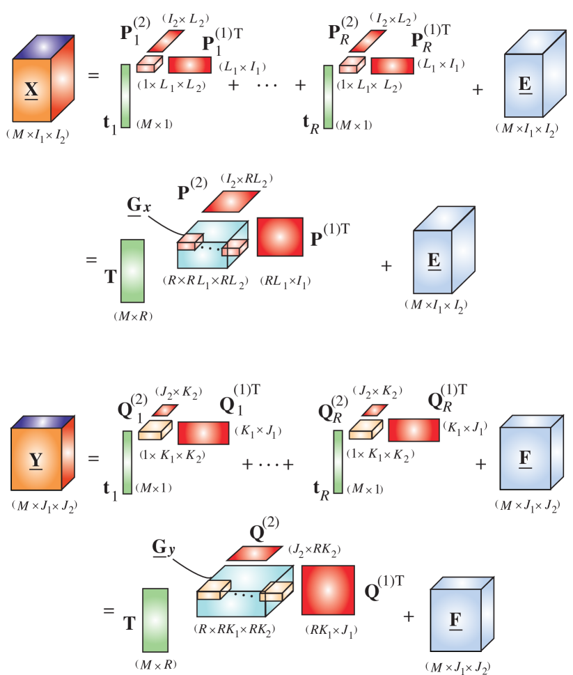
Figure 2.4: The HOPLS model which approximates the independent variables, $\underline{\mathbf{X}}$, as a sum of rank-$(1,L_{1},L_{2})$ tensors. The approximation for the dependent variables, $\underline{\mathbf{Y}}$, follows a similar principle, whereby the common latent components, $\mathbf{T}$, are shared between $\underline{\mathbf{X}}$ and $\underline{\mathbf{Y}}$.

Benefiting from the advantages of Tucker decomposition over the CP model, HOPLS generates approximate latent components that better model the data than $N$-way PLS. Specifically, the HOPLS differs substantially from the $N$-way PLS model in the sense that the sizes of loading matrices are controlled by a hyperparameter, providing a tradeoff between the model fit and model complexity. Note that HOPLS simplifies into $N$-way PLS if we impose the rank-1 constraints for the Tucker blocks, that is $\forall n:\{L_{n}\}=1$ and $\forall m:\{K_{m}\}=1$.

The optimization of subspace transformation according to (2.33) can be formulated as a problem of determining a set of orthogonal loadings and latent vectors. Since these terms can be optimized sequentially, using the same criteria and based on deflation, in the following, we shall illustrate the procedure based on finding the first latent vector, $\mathbf{t}$, and two sequences of loading matrices, $\mathbf{P}^{(n)}$ and $\mathbf{Q}^{(n)}$. Finally, we shall denote tensor contraction in mode one by $\langle\underline{\mathbf{X}},\underline{\mathbf{Y}}\rangle_{\{1;1\}}$, so that the cross-covariance tensor is defined by

$$\underline{\mathbf{C}}=\mbox{COV}_{\{1;1\}}(\underline{\mathbf{X}},\underline{\mathbf{Y}})\in\mathbb{R}^{I_{1}\times\cdots\times I_{N}\times J_{1}\times\cdots\times J_{N}}.$$ (2.36)

The above optimization problem can now be formulated as

$$\!\!\!\!\max_{\left\{\mathbf{P^{(n)}},\mathbf{Q^{(n)}}\right\}} \left\|[\![\underline{\mathbf{C}};\mathbf{P}^{(1)\,\text{T}},\!\ldots,\!\mathbf{P}^{(N)\,\text{T}},\mathbf{Q}^{(1)\,\text{T}},\!\ldots\!,\mathbf{Q}^{(N)\,\text{T}}]\!]\right\|_{F}^{2}$$

s.t. $$\mathbf{P}^{(n)\,\text{T}}\mathbf{P}^{(n)}=\mathbf{I}_{L_{n}},\quad\mathbf{Q}^{(n)\,\text{T}}\mathbf{Q}^{(n)}=\mathbf{I}_{K_{n}},$$ (2.37)

where $[\![\ldots]\!]$ denotes the multilinear products between a tensor and a set of matrices, $\mathbf{P}^{(n)}$ and $\mathbf{Q}^{(n)},\;n=1,\ldots,N$, comprise the unknown parameters. This is equivalent to finding the best subspace approximation of $\underline{\mathbf{C}}$ which can be obtained by rank-($L_{1},\ldots,L_{N},K_{1},\ldots,K_{N}$) HOSVD of tensor $\underline{\mathbf{C}}$. The higher-order orthogonal iteration (HOOI) algorithm, which is known to converge fast, can be employed to find the parameters $\mathbf{P}^{(n)}$ and $\mathbf{Q}^{(n)}$ by orthogonal Tucker decomposition of $\underline{\mathbf{C}}$. The detailed procedure of HOPLS is shown in Algorithm 4.

The prediction for a new sample set $\underline{\mathbf{X}}^{*}$ is then performed as $\mathbf{Y}_{(1)}^{*}\approx\mathbf{X}_{(1)}^{*}\mathbf{W}^{x}\mathbf{W}^{y}$, where the $r$th column of $\mathbf{W}^{x}_{r}$ is given by $\mathbf{w}^{x}_{r}=(\mathbf{P}_{r}^{(N)}\otimes\cdots\otimes\mathbf{P}^{(1)}_{r}){\mathbf{G}_{x}}_{r(1)}^{\dagger}$ and the $r$th row of $\mathbf{W}^{y}_{r}$ is given by $\mathbf{w}^{y}_{r}={\mathbf{G}_{y}}_{r(1)}^{\dagger}(\mathbf{Q}_{r}^{(N)}\otimes\cdots\otimes\mathbf{Q}^{(1)}_{r})^{\text{T}}$.

0:  $\underline{\mathbf{X}}\in\mathbb{R}^{M\times I_{1}\times I_{2}\times\cdots\times I_{N}}$ and $\underline{\mathbf{Y}}\in\mathbb{R}^{M\times J_{1}\times J_{2}\times\cdots\times J_{N}}$. 0:  $\{\mathbf{P}_{r}^{(n)}\}$, $\{\mathbf{Q}_{r}^{(n)}\}$, $\{{\underline{\mathbf{G}}_{x}}_{r}\}$, $\{{\underline{\mathbf{G}}_{y}}_{r}\}$, $\mathbf{T}$, $n=1,\ldots,N,r=1,\ldots,R$. 1:  for $r=1$ to $R$ do 2:     $\underline{\mathbf{C}}\leftarrow\text{COV}_{1;1}(\underline{\mathbf{X}},\underline{\mathbf{Y}})\in\mathbb{R}^{I_{1}\times\cdots\times I_{N}\times J_{1}\times\cdots\times J_{N}}$ 3:     Compute $\{\mathbf{P}_{r}^{(n)}\}$ and $\{\mathbf{Q}_{r}^{(n)}\}$ by HOOI decomposition of $\underline{\mathbf{C}}$. 4:     $\mathbf{t}_{r}\leftarrow$ the principal eigenvector of $\underline{\mathbf{X}}\times_{2}\mathbf{P}_{r}^{(1)}\cdots\times_{N+1}\mathbf{P}^{(N)}_{r}$ 5:     ${\underline{\mathbf{G}}_{x}}_{r}\leftarrow\underline{\mathbf{X}}\bar{\times}_{1}\mathbf{t}_{r}\times_{2}\mathbf{P}_{r}^{(1)\,\text{T}}\cdots\times_{N+1}\mathbf{P}^{(N)\,\text{T}}_{r}$ 6:     ${\underline{\mathbf{G}}_{y}}_{r}\leftarrow\underline{\mathbf{Y}}\bar{\times}_{1}\mathbf{t}_{r}\times_{2}\mathbf{Q}_{r}^{(1)\,\text{T}}\cdots\times_{N+1}\mathbf{Q}^{(N)\,\text{T}}_{r}$ 7:     Deflation: $\underline{\mathbf{X}}\leftarrow\underline{\mathbf{X}}-{\underline{\mathbf{G}}_{x}}_{r}\times_{1}\mathbf{t}_{r}\times_{2}\mathbf{P}_{r}^{(1)}\cdots\times_{N+1}\mathbf{P}^{(N)}_{r}$ 8:     Deflation: $\underline{\mathbf{Y}}\leftarrow\underline{\mathbf{Y}}-{\underline{\mathbf{G}}_{y}}_{r}\times_{1}\mathbf{t}_{r}\times_{2}\mathbf{Q}_{r}^{(1)}\cdots\times_{N+1}\mathbf{Q}^{(N)}_{r}$ 9:  end for

Algorithm 4 Higher-Order Partial Least Squares (HOPLS)

2.6 Kernel HOPLS

We next briefly introduce the concept of kernel-based tensor PLS (KTPLS or KHOPLS) [Zhao et al., 2013c, Hou et al., 2016b], as a natural extension of the HOPLS to possibly infinite dimensional and nonlinear kernel spaces. Consider $N$ pairs of tensor observations $\{(\underline{\mathbf{X}}_{m},\underline{\mathbf{Y}}_{m})\}_{m=1}^{M}$, where $\underline{\mathbf{X}}_{m}$ denotes an $N$th-order independent tensor and $\underline{\mathbf{Y}}_{m}$ an $L$th-order dependent tensor. Note that the data tensors, $\underline{\mathbf{X}}_{m}$ and $\underline{\mathbf{Y}}_{m}$, can be concatenated to form an $(N+1)$th-order tensor $\underline{\mathbf{X}}\in\mathbb{R}^{M\times I_{1}\times\cdots\times I_{N}}$ and $(L+1)$th-order tensor $\underline{\mathbf{Y}}\in\mathbb{R}^{M\times J_{1}\times\cdots\times J_{L}}$. Within the kernel framework, the data tensors $\underline{\mathbf{X}}$ and $\underline{\mathbf{Y}}$ are mapped onto the Hilbert space by a reproducing kernel mapping $\phi:\quad\underline{\mathbf{X}}_{m}$ $\longmapsto\phi\left(\underline{\mathbf{X}}_{m}\right)$. For simplicity, we shall denote $\phi(\underline{\mathbf{X}})$ by $\underline{\boldsymbol{\Phi}}$ and $\phi(\underline{\mathbf{Y}})$ by $\underline{\boldsymbol{\Psi}}$. The KTPLS then aims to perform the tensor decompositions, corresponding to those in (2.35), such that

$$\begin{split}\underline{\boldsymbol{\Phi}}&=\underline{\mathbf{G}}_{\underline{\mathbf{X}}}\times_{1}\mathbf{T}\times_{2}{\mathbf{P}}^{(1)}\cdots\times_{N+1}{\mathbf{P}}^{(N)}+\underline{\mathbf{E}}_{\underline{\mathbf{X}}},\\ \underline{\boldsymbol{\Psi}}&=\underline{\mathbf{G}}_{\underline{\mathbf{Y}}}\times_{1}\mathbf{U}\times_{2}{\mathbf{Q}}^{(1)}\cdots\times_{L+1}{\mathbf{Q}}^{(L)}+\underline{\mathbf{E}}_{\underline{\mathbf{Y}}},\\ \mathbf{U}&=\mathbf{TD}+\mathbf{E}_{U}.\end{split}$$ (2.38)

Since within the kernel framework, the tensors $\widetilde{\underline{\mathbf{G}}}_{\underline{\mathbf{X}}}=\underline{\mathbf{G}}_{\underline{\mathbf{X}}}\times_{2}{\mathbf{P}}^{(1)}\cdots\times_{N+1}{\mathbf{P}}^{(N)}$ and $\widetilde{\underline{\mathbf{G}}}_{\underline{\mathbf{Y}}}=\underline{\mathbf{G}}_{\underline{\mathbf{Y}}}\times_{2}{\mathbf{Q}}^{(1)}\cdots\times_{L+1}{\mathbf{Q}}^{(L)}$ can be respectively represented as a linear combination of $\{\phi(\underline{\mathbf{X}}_{m})\}$ and $\{\phi(\underline{\mathbf{Y}}_{m})\}$, i.e., $\widetilde{\underline{\mathbf{G}}}_{\underline{\mathbf{X}}}=\boldsymbol{\Phi}\times_{1}\mathbf{T}^{\text{T}}$ and $\widetilde{\underline{\mathbf{G}}}_{\underline{\mathbf{Y}}}=\boldsymbol{\Psi}\times_{1}\mathbf{U}^{\text{T}}$, for the KTPLS solution we only need to find the latent vectors of $\mathbf{T}=[\mathbf{t}_{1},\ldots,\mathbf{t}_{R}]$ and $\mathbf{U}=[\mathbf{u}_{1},\ldots,\mathbf{u}_{R}]$, such that they exhibit maximum pair-wise covariance, through solving sequentially the following optimization problems

$$\max_{\{\mathbf{w}^{(n)}_{r},\mathbf{v}^{(l)}_{r}\}}\quad[\mbox{cov}(\mathbf{t}_{r},\mathbf{u}_{r})]^{2},$$ (2.39)

where

$$\begin{split}&\mathbf{t}_{r}=\underline{\boldsymbol{\Phi}}\bar{\times}_{2}\mathbf{w}^{(1)}_{r}\cdots\bar{\times}_{N+1}\mathbf{w}^{(N)}_{r},\\ &\mathbf{u}_{r}=\underline{\boldsymbol{\Psi}}\bar{\times}_{2}\mathbf{v}^{(1)}_{r}\cdots\bar{\times}_{L+1}\mathbf{v}^{(L)}_{r}.\end{split}$$ (2.40)

Upon rewriting (2.40) in a matrix form, this yields $\mathbf{t}_{r}=\boldsymbol{\Phi}_{(1)}\widetilde{\mathbf{w}}_{r}$ where $\widetilde{\mathbf{w}}_{r}=\mathbf{w}_{r}^{(N)}\otimes\cdots\otimes\mathbf{w}_{r}^{(1)}$ and $\mathbf{u}_{r}=\boldsymbol{\Psi}_{(1)}\widetilde{\mathbf{v}}_{r}$ where $\widetilde{\mathbf{v}}_{r}=\mathbf{v}_{r}^{(N)}\otimes\cdots\otimes\mathbf{v}_{r}^{(1)}$, which can be solved by a kernelized version of the eigenvalue problem, i.e., $\boldsymbol{\Phi}_{{(1)}}\boldsymbol{\Phi}_{(1)}^{\text{T}}\boldsymbol{\Psi}_{(1)}\boldsymbol{\Psi}_{(1)}^{\text{T}}\mathbf{t}_{r}=\lambda\mathbf{t}_{r}$ and $\mathbf{u}_{r}=\boldsymbol{\Psi}_{(1)}\boldsymbol{\Psi}_{(1)}^{\text{T}}\mathbf{t}_{r}$ [Rosipal and Trejo, 2002]. Note that since the term $\boldsymbol{\Phi}_{{(1)}}\boldsymbol{\Phi}_{(1)}^{\text{T}}$ contains only the inner products between vectorized input tensors, it can be replaced by an $M\times M$ kernel matrix $\mathbf{K}_{\underline{\mathbf{X}}}$, to give $\mathbf{K}_{\underline{\mathbf{X}}}\mathbf{K}_{\underline{\mathbf{Y}}}\mathbf{t}_{r}=\lambda\mathbf{t}_{r}$ and $\mathbf{u}_{r}=\mathbf{K}_{\underline{\mathbf{Y}}}\mathbf{t}_{r}$.

In order to exploit the rich multilinear structure of tensors, kernel matrices should be computed using the kernel functions for tensors, i.e., $(\mathbf{K}_{\underline{\mathbf{X}}})_{mm^{\prime}}=k\left(\underline{\mathbf{X}}_{m},\underline{\mathbf{X}}_{m^{\prime}}\right)$ and $(\mathbf{K}_{\underline{\mathbf{Y}}})_{mm^{\prime}}=k\left(\underline{\mathbf{Y}}_{m},\underline{\mathbf{Y}}_{m^{\prime}}\right)$ (for more details see Section 2.7).

Finally, for a new data sample, $\underline{\mathbf{X}}^{*}$, the prediction of $\mathbf{y}$, denoted by $\mathbf{y}^{*}$ is performed by computing the vector

$$\mathbf{y}^{*T}=\mathbf{k}^{*T}\mathbf{U}(\mathbf{T}^{\text{T}}\mathbf{K}_{\underline{\mathbf{X}}}\mathbf{U})^{-1}\mathbf{T}^{\text{T}}\mathbf{Y}_{(1)},$$ (2.41)

where $(\mathbf{k}^{*})_{m}=k\left(\underline{\mathbf{X}}_{m},\underline{\mathbf{X}}^{*}\right)$ and the vector $\mathbf{y}^{*}$ can be reshaped to a tensor $\underline{\mathbf{Y}}^{*}$. The detailed procedure of KHOPLS is shown in Algorithm 5.

0:  $\underline{\mathbf{X}}\in\mathbb{R}^{M\times I_{1}\times I_{2}\times\cdots\times I_{N}}$ and $\underline{\mathbf{Y}}\in\mathbb{R}^{M\times J_{1}\times I_{2}\times\cdots\times J_{L}}$. 0:  $\mathbf{T},\mathbf{U},\mathbf{K}_{\underline{\mathbf{X}}}$. 1:  Compute kernel matrix $\mathbf{K}_{\underline{\mathbf{X}}}$ and $\mathbf{K}_{\underline{\mathbf{Y}}}$ by using tensor kernel functions 2:  Compute $\mathbf{t}_{r}$ by solving $\mathbf{K}_{\underline{\mathbf{X}}}\mathbf{K}_{\underline{\mathbf{Y}}}\mathbf{t}_{r}=\lambda\mathbf{t}_{r}$, $r=1,\ldots,R$ 3:  $\mathbf{u}_{r}=\mathbf{K}_{\underline{\mathbf{Y}}}\mathbf{t}_{r}$, $r=1,\ldots,R$ 4:  $\mathbf{T}=[\mathbf{t}_{1},\ldots,\mathbf{t}_{R}]$ and $\mathbf{U}=[\mathbf{u}_{1},\ldots,\mathbf{u}_{R}]$

Algorithm 5 Kernel Higher-Order Partial Least Squares (KHOPLS)

The intuitive interpretation of (2.41) can take several forms: i) as a linear combination of $M$ observations $\{\underline{\mathbf{Y}}_{m}\}$ and the coefficients $\mathbf{k}^{*T}\mathbf{U}(\mathbf{T}^{\text{T}}\mathbf{K}_{\underline{\mathbf{X}}}\mathbf{U})^{-1}\mathbf{T}^{\text{T}}$; ii) as a linear combination of $M$ kernels, each centered around a training point, i.e., $y_{j}^{*}=\sum_{m=1}^{M}\alpha_{m}k\left(\underline{\mathbf{X}}_{m},\underline{\mathbf{X}}^{*}\right)$, where $\alpha_{m}=\left(\mathbf{U}(\mathbf{T}^{\text{T}}\mathbf{K}_{\underline{\mathbf{X}}}\mathbf{U})^{-1}\mathbf{T}^{\text{T}}\mathbf{Y}_{(1)}\right)_{mj}$; iii) the vector $\mathbf{t}^{*}$ is obtained by nonlinearly projecting the tensor $\underline{\mathbf{X}}^{*}$ onto the latent space spanned by $\mathbf{t}^{*T}=\mathbf{k}^{*T}\mathbf{U}(\mathbf{T}^{\text{T}}\mathbf{K}_{\underline{\mathbf{X}}}\mathbf{U})^{-1}$, then $\mathbf{y}^{*T}$ is predicted by a linear regression against $\mathbf{t}^{*}$, i.e., $\mathbf{y}^{*T}=\mathbf{t}^{*T}\mathbf{C}$, where the regression coefficients are given by the matrix $\mathbf{C}=\mathbf{T}^{\text{T}}\mathbf{Y}_{(1)}$.

Note that, in general, to ensure a strict linear relationship between the latent vectors and output in the original spaces, the kernel functions for data $\underline{\mathbf{Y}}$ are restricted to linear kernels.

2.7 Kernel Functions in Tensor Learning

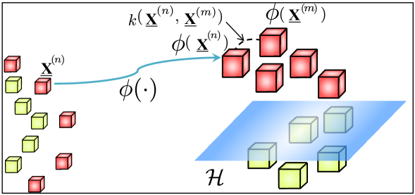
Figure 2.5: The concept of kernel learning for tensors. Tensor observations are mapped into the reproducing kernel Hilbert space $\mathcal{H}$ by a nonlinear mapping function $\phi(\cdot)$. The kernel function serves as a similarity measure between two tensors.

Kernel functions can be considered as a means for defining a new topology which implies a priori knowledge about the invariance in the input space [Schölkopf and Smola, 2002] (see Figure 2.5). Kernel algorithms can also be used for estimation of vector-valued nonlinear and nonstationary signals [Tobar et al., 2014]. In this section, we discuss the kernels for tensor-valued inputs, which should exploit multi-way structures while maintaining the notion of similarity measures.

Most straightforward tensor-valued reproducing kernels are a direct generalization from vectors to $N$th-order tensors, such as the following kernel functions $k:\underline{\mathbf{X}}\times\underline{\mathbf{X}}\rightarrow\mathbb{R}$, given by

$$\begin{split}&\mbox{Linear kernel:}\quad k(\underline{\mathbf{X}},\underline{\mathbf{X}}^{\prime})=\langle\mbox{vec}(\underline{\mathbf{X}}),\mbox{vec}(\underline{\mathbf{X}}^{\prime})\rangle,\\ &\mbox{Gaussian-RBF kernel:}\quad k(\underline{\mathbf{X}},\underline{\mathbf{X}}^{\prime})=\mbox{exp}\left(-\frac{1}{2\beta^{2}}\|\underline{\mathbf{X}}-\underline{\mathbf{X}}^{\prime}\|_{F}^{2}\right).\end{split}$$ (2.42)

In order to define a similarity measure that directly exploits the multilinear algebraic structure of input tensors, Signoretto et al. [2011, 2012] proposed a tensorial kernel which both exploits the algebraic geometry of tensors spaces and provides a similarity measure between the different subspaces spanned by higher-order tensors. Another such kernel is the product kernel which can be defined by $N$ factor kernels, as $k(\underline{\mathbf{X}},\underline{\mathbf{X^{\prime}}})=\prod_{n=1}^{N}k\left(\mathbf{X}_{(n)},\mathbf{X^{\prime}}_{(n)}\right)$, where each factor kernel represents a similarity measure between mode-$n$ matricizations of two tensors, $\underline{\mathbf{X}}$ and $\underline{\mathbf{X^{\prime}}}$.

One similarity measure between matrices is the so called Chordal distance, which is a projection of the Frobenius norm on a Grassmannian manifolds [Signoretto et al., 2011]. For example, for an $N$th-order tensor, $\underline{\mathbf{X}}$, upon the applications of SVD to its mode-$n$ unfolding, that is, $\mathbf{X}_{(n)}=\mathbf{U}_{\mathbf{X}}^{(n)}\mathbf{\Sigma}^{(n)}_{\mathbf{X}}\mathbf{V}^{(n)\,\text{T}}_{\mathbf{X}}$, the Chordal distance-based kernel for tensorial data is defined as

$$k(\underline{\mathbf{X}},\underline{\mathbf{X^{\prime}}})=\prod_{n=1}^{N}\mbox{exp}\left(-\frac{1}{2\beta^{2}}\left\|\mathbf{V}^{(n)}_{\mathbf{X}}\mathbf{V}^{(n)\,\text{T}}_{\mathbf{X}}-\mathbf{V}^{(n)}_{\mathbf{X}^{\prime}}\mathbf{V}^{(n)\,\text{T}}_{\mathbf{X}^{\prime}}\right\|_{F}^{2}\right),$$ (2.43)

where $\beta$ is a kernel parameter. It should be emphasized that such a tensor kernel ensures (provides) rotation and reflection invariance for elements on the Grassmann manifold [Signoretto et al., 2011].

Zhao et al. [2013c] proposed a whole family of probabilistic product kernels based on generative models. More specifically, an $N$th-order tensor-valued observation is first mapped onto an $N$-dimensional model space, then information divergence is applied as a similarity measure in such a model space (see also [Cichocki et al., 2011, 2015]).

The advantage of probabilistic tensor kernels is that they can deal with multiway data with missing values and with variable data length. Given that probabilistic kernels provide a way to model one tensor from $N$ different viewpoints which correspond to different lower-dimensional vector spaces, this makes it possible for multiway relations to be captured within a similarity measure.

A general similarity measure between two tensors, $\underline{\mathbf{X}}$ and $\underline{\mathbf{X}}^{\prime}$, in mode-$n$ can be defined as

$$S_{n}(\underline{\mathbf{X}}\|\underline{\mathbf{X}}^{\prime})=D\left(p(\mathbf{x}|\boldsymbol{\Omega}_{n}^{\underline{\mathbf{X}}})\|q(\mathbf{x}|\boldsymbol{\Omega}^{\underline{\mathbf{X}}^{\prime}}_{n})\right),$$ (2.44)

where $p$ and $q$ are distributions which respectively represent the probability density function for $\underline{\mathbf{X}}$ and $\underline{\mathbf{X}}^{\prime}$, $D(p\|q)$ is an information divergence between two distributions, while $\Omega_{n}^{\underline{\mathbf{X}}}$ denotes the parameters of a mode-$n$ distribution of $\underline{\mathbf{X}}$, which depends on the model assumption.

For simplicity, we usually assume Gaussian models for all modes of tensor $\underline{\mathbf{X}}$, so that $\Omega$ can be expressed by the mean values and covariance matrices of that distribution. One simple and very useful information divergence is the standard symmetric Kullback-Leibler (sKL) divergence [Moreno et al., 2003], expressed as

$$\begin{split}D_{sKL}\left(p(\mathbf{x}|\boldsymbol{\lambda})\|q(\mathbf{x}|\boldsymbol{\lambda}^{\prime})\right)&=\frac{1}{2}\int_{-\infty}^{+\infty}p(\mathbf{x}|\boldsymbol{\lambda})\log\frac{p(\mathbf{x}|\boldsymbol{\lambda})}{q(\mathbf{x}|\boldsymbol{\lambda}^{\prime})}d\mathbf{x}\\ &+\frac{1}{2}\int_{-\infty}^{+\infty}q(\mathbf{x}|\boldsymbol{\lambda}^{\prime})\log\frac{q(\mathbf{x}|\boldsymbol{\lambda}^{\prime})}{p(\mathbf{x}|\boldsymbol{\lambda})}d\mathbf{x},\end{split}$$ (2.45)

where $\boldsymbol{\lambda}$ and $\boldsymbol{\lambda}^{\prime}$ are parameters of the probability distributions. An alternative simple divergence is the symmetric Jensen-Shannon (JS) divergence [Chan et al., 2004, Endres and Schindelin, 2003, Cichocki et al., 2011], given by

$$D_{JS}(p\|q)=\frac{1}{2}\text{KL}(p\|r)+\frac{1}{2}\text{KL}(q\|r),$$ (2.46)

where $\text{KL}(\cdot\|\cdot)$ denotes the Kullback-Leibler divergence and $r(\mathbf{x})=\frac{p(\mathbf{x})+q(\mathbf{x})}{2}$.

Table 2.1: Kernel functions for tensor

$k(\underline{\mathbf{X}},\underline{\mathbf{Y}})=\Big{\langle}\Phi(\text{vec}(\underline{\mathbf{X}})),\Phi(\text{vec}(\underline{\mathbf{Y}}))\Big{\rangle}$ $k(\underline{\mathbf{X}},\underline{\mathbf{Y}})=\Big{\langle}\Phi(\mathbf{X}_{(1)},\ldots,\mathbf{X}_{(N)}),\Phi(\mathbf{Y}_{(1)},\ldots,\mathbf{Y}_{(N)})\Big{\rangle}$ $k(\underline{\mathbf{X}},\underline{\mathbf{Y}})=\Big{\langle}\Phi(\underline{\mathbf{X}}^{{}^{\prime}}),\Phi(\underline{\mathbf{Y}}^{{}^{\prime}})\Big{\rangle}$ , where $\underline{\mathbf{X}}^{{}^{\prime}}$ is a CP decomposition of $\underline{\mathbf{X}}$ $k(\underline{\mathbf{X}},\underline{\mathbf{Y}})=\Big{\langle}\Phi\big{(}\underline{\mathbf{G}}_{X}^{(1)},\ldots,\underline{\mathbf{G}}_{X}^{(N)}\big{)},\Phi\big{(}\underline{\mathbf{G}}_{Y}^{(1)},\ldots,\underline{\mathbf{G}}_{Y}^{(N)}\big{)}\Big{\rangle}$ where $\underline{\mathbf{G}}_{X}^{(1)},\ldots,\underline{\mathbf{G}}_{X}^{(N)}$ are cores obtained by TT decomposition of $\underline{\mathbf{X}}$, and $\underline{\mathbf{G}}_{Y}^{(1)},\ldots,\underline{\mathbf{G}}_{Y}^{(N)}$ are cores obtained by TT decomposition of $\underline{\mathbf{Y}}$.

In summary, a probabilistic product kernel for tensors can be defined as

$$k(\underline{\mathbf{X}},\underline{\mathbf{X}}^{\prime})=\alpha^{2}\prod_{n=1}^{N}\mbox{exp}\left(-\frac{1}{2\beta_{n}^{2}}S_{n}(\underline{\mathbf{X}}\|\underline{\mathbf{X}}^{\prime})\right),$$ (2.47)

where $S_{n}(\underline{\mathbf{X}}\|\underline{\mathbf{X}}^{\prime})$ is a suitably chosen probabilistic divergence, $\alpha$ denotes a magnitude parameter and $[\beta_{1},\ldots,\beta_{N}]$ are length-scale parameters.

An intuitive interpretation of the kernel function in (2.47) is that $N$th-order tensors are assumed to be generated from $N$ generative models, while the similarity of these models, measured by information divergence, is employed to provide a multiple kernel with well defined properties and conditions. This kernel can then effectively capture the statistical properties of tensors, which promises to be a powerful tool for multidimensional structured data analysis, such as video classification and multichannel feature extraction from brain electrophysiological responses.

There are many possibilities to define kernel functions for tensors, as outlined in Table 2.1 and Figure 2.6.

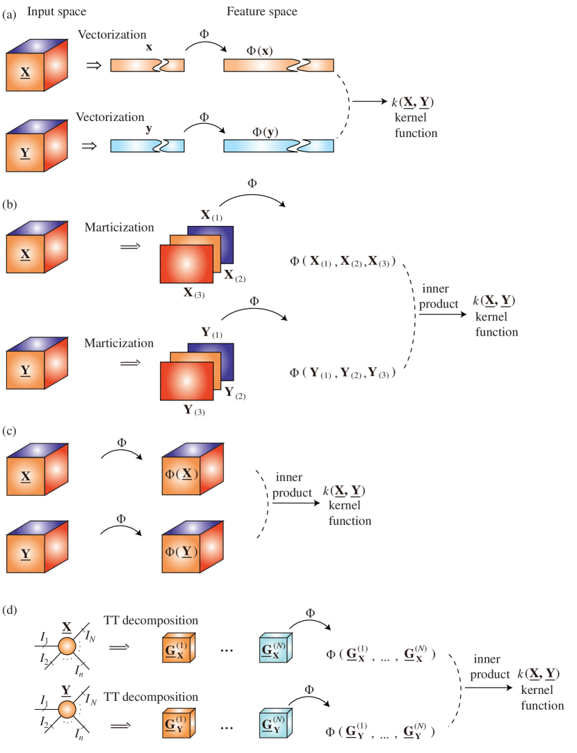
Figure 2.6: Approaches for the construction of tensor kernel functions. The kernel function can be defined based on (a) vectorization of data tensors, (b) matricization of data tensors, (c) raw tensors format (direct approach), and (d) core tensors from low-rank tensor decompositions.

2.8 Tensor Variate Gaussian Processes (TVGP)

Gaussian processes (GP) can be considered as a class of probabilistic models which specify a distribution over a function space, where the inference is performed directly in the function space [Rasmussen and Williams, 2006]. The GP model for tensor-valued input spaces, called the Tensor-based Gaussian Processes (Tensor-GP), is designed so as to take into account the tensor structure of data [Zhao et al., 2013c, 2014, Hou et al., 2015].

Given a paired dataset of $M$ observations $\mathcal{D}=\{(\underline{\mathbf{X}}_{m},y_{m})|m=1,\ldots,M\}$, the tensor inputs for all $M$ instances (cases) are aggregated into an $(N+1)$th-order design concatenated tensor $\underline{\mathbf{X}}\in\mathbb{R}^{M\times I_{1}\times\cdots\times I_{N}}$, while the targets are collected in the vector $\mathbf{y}=[y_{1},\ldots,y_{M}]^{\text{T}}$. After observing the training data $\mathcal{D}=\{\underline{\mathbf{X}},\mathbf{y}\}$, the aim is to make inferences about the relationship between the inputs $\underline{{\bf X}}$ and targets (output $\mathbf{y}$), i.e., to perform estimation of the conditional distribution of the targets given the inputs, and in doing so to perform the prediction based on a new input, $\underline{\mathbf{X}}_{*}$, which has not been seen in the training set.

The distribution of observations can be factored over cases in the training set by $\mathbf{y}\sim\prod_{m=1}^{M}\mathcal{N}(y_{m}|f_{m},\sigma^{2}),$ where $f_{m}$ denotes the latent function $f(\underline{\mathbf{X}}_{m})$, and $\sigma^{2}$ denotes noise variance.

A Gaussian process prior can be placed over the latent function, which implies that any finite subset of latent variables has a multivariate Gaussian distribution, denoted by

$$f(\underline{\mathbf{X}})\sim\mathcal{GP}(m(\underline{\mathbf{X}}),k(\underline{\mathbf{X}},\underline{\mathbf{X^{\prime}}})\mid\boldsymbol{\theta}),$$ (2.48)

where $m(\underline{\mathbf{X}})$ is the mean function which is usually set to zero for simplicity, and $k(\underline{\mathbf{X}},\underline{\mathbf{X^{\prime}}})$ is the covariance function (e.g., kernel function) for tensor data, with a set of hyper-parameters denoted by $\boldsymbol{\theta}$.

The hyper-parameters from the observation model and the GP prior are collected in $\Theta=\{\sigma,\boldsymbol{\theta}\}$. The model is then hierarchically extended to the third level by also giving priors over the hyperparameters in $\Theta$.

To incorporate the knowledge that the training data provides about the function $\mathbf{f}(\underline{\mathbf{X}})$, we can use the Bayes rule to infer the posterior of the latent function $\mathbf{f}(\underline{\mathbf{X}})=[f(\underline{\mathbf{X}}_{1}),\ldots,f(\underline{\mathbf{X}}_{M})]^{\text{T}}$ by

$$p\left(\mathbf{f}\middle|\mathcal{D},\Theta\right)=\frac{p\left(\mathbf{y}\middle|\mathbf{f},\sigma\right)p\left(\mathbf{f}\middle|\underline{\mathbf{X}},\theta\right)}{\int p\left(\mathbf{y}\middle|\mathbf{f},\sigma\right)p\left(\mathbf{f}\middle|\underline{\mathbf{X}},\theta\right)d\mathbf{f}},$$ (2.49)

where the denominator in (2.49) can be interpreted as the marginal likelihood obtained by the integration over $\mathbf{f}$, to yield

$$\mathbf{y}|\underline{\mathbf{X}},\theta,\sigma^{2}\sim\mathcal{N}(\mathbf{y}|\mathbf{0},\mathbf{K}+\sigma^{2}\mathbf{I}),$$ (2.50)

where $(\mathbf{K})_{ij}=k(\underline{\mathbf{X}}_{i},\underline{\mathbf{X}}_{j})$ denotes the covariance matrix or kernel matrix.

Note that, since the Gaussian observation model is analytically tractable and so it avoids the approximate inference, the conditional posterior of the latent function $\mathbf{f}$ is Gaussian, and the posterior of $f_{*}$ is also Gaussian, together with the observation $y_{*}$.

Finally, the predictive distribution of $y_{*}$ corresponding to $\underline{\mathbf{X}}_{*}$ can be inferred as $y_{*}|\underline{\mathbf{X}}_{*},\underline{\mathbf{X}},\mathbf{y},\Theta\sim\mathcal{N}(\overline{y}_{*},\mbox{cov}(y_{*}))$, where

$$\begin{split}\overline{y}^{*}&=k(\underline{\mathbf{X}}_{*},\underline{\mathbf{X}})(k(\underline{\mathbf{X}},\underline{\mathbf{X}})+\sigma_{n}^{2}\mathbf{I})^{-1}\mathbf{y},\\ \mbox{cov}(y^{*})&=k(\underline{\mathbf{X}}_{*},\underline{\mathbf{X}}_{*})-k(\underline{\mathbf{X}}_{*},\underline{\mathbf{X}})(k(\underline{\mathbf{X}},\underline{\mathbf{X}})+\sigma^{2}\mathbf{I})^{-1}k(\underline{\mathbf{X}},\underline{\mathbf{X}}_{*}).\end{split}$$ (2.51)

The classification problem consisting of $N$th-order tensors $\underline{\mathbf{X}}_{m}\in\mathbb{R}^{I_{1}\times\cdots\times I_{N}}$ which are associated with target classes $y_{m}\in\{1,\ldots,C\}$, where $C>2$ and $m=1,\ldots,M$, was investigated by Zhao et al. [2013b]. All class labels are collected in the $M\times 1$ target vector $\mathbf{y}$, and all tensors are concatenated in an $(N+1)$th-order tensor $\underline{\mathbf{X}}$ of size $M\times I_{1}\times\cdots\times I_{N}$. Given the latent function $\mathbf{f}_{m}=[{f}_{m}^{1},{f}_{m}^{2},\ldots,{f}_{m}^{C}]^{\text{T}}=\mathbf{f}(\underline{\mathbf{X}}_{m})$ at the observed input location $\underline{\mathbf{X}}_{m}$, the class labels $y_{m}$ are assumed to be independent and identically distributed, as defined by a multinomial probit likelihood model $p(y_{m}|\mathbf{f})$. The latent vectors from all observations are denoted by $\mathbf{f}=[f_{1}^{1},\ldots,f_{M}^{1},f_{1}^{2},\ldots,f_{M}^{2},\ldots,$ $f_{1}^{C},\ldots,f_{M}^{C}]^{\text{T}}$.

The objective of TVGP is to predict the class membership for a new input tensor, $\underline{\mathbf{X}}_{*}$, given the observed data, $\mathcal{D}=\{\underline{\mathbf{X}},\mathbf{y}\}$. Gaussian process priors are placed on the latent function related to each class, which is the common assumption in multi-class GP classification (see [Rasmussen and Williams, 2006, Riihimäki et al., 2012]).

Such a specification results in the zero-mean Gaussian prior for $\mathbf{f}$, given by

$$p(\mathbf{f}|\underline{\mathbf{X}})=\mathcal{N}(\mathbf{0},\mathbf{K}),$$ (2.52)

where $\mathbf{K}$ is a $CM\times CM$ block-diagonal covariance matrix and every matrix $\mathbf{K}^{1},\ldots,\mathbf{K}^{C}$ (of size $M\times M$) on its diagonal corresponds to each class. The element $K_{i,j}^{c}$ in a $c$th class covariance matrix defines the prior covariance between $f_{i}^{c}$ and $f_{j}^{c}$, which is governed by a kernel function $k(\underline{\mathbf{X}}_{i},\underline{\mathbf{X}}_{j})$, i.e., $K_{i,j}^{c}=k(\underline{\mathbf{X}}_{i},\underline{\mathbf{X}}_{j})=\text{Cov}(f_{i}^{c},f_{j}^{c})$ within the class $c$. Note that since the kernel function should be defined in tensor-variate input space, hence commonly used kernel functions, such as Gaussian RBF, are infeasible. Therefore, the framework of probabilistic product kernel for tensors, described in Sec.2.7, should be applied. In a kernel function, the hyperparameters are defined so as to control the smoothness properties and overall variance of latent functions, and are usually combined into one vector $\boldsymbol{\theta}$. For simplicity, we use the same $\boldsymbol{\theta}$ for all classes. For the likelihood model, we consider the multinomial probit, which is a generalization of the probit model, given by

$$p(y_{m}|\mathbf{f}_{m})=\text{E}_{p(u_{m})}\left\{\prod_{c=1,c\neq y_{m}}^{C}\Phi(u_{m}+f_{m}^{y_{m}}-f_{m}^{c})\right\},$$ (2.53)

where $\Phi$ denotes the cumulative distribution function of the standard normal distribution, and the auxiliary variable $u_{m}$ is distributed as $p(u_{m})=\mathcal{N}(0,1)$.

By applying the Bayes theorem, the posterior distribution of the latent function is given by

$$p(\mathbf{f}|\mathcal{D},\boldsymbol{\theta})=\frac{1}{Z}p(\mathbf{f}|\underline{\mathbf{X}},\boldsymbol{\theta})\prod_{m=1}^{M}p(y_{m}|\mathbf{f}_{m}),$$ (2.54)

where $Z=\int p(\mathbf{f}|\underline{\mathbf{X}},\boldsymbol{\theta})\prod_{m=1}^{M}p(y_{m}|\mathbf{f}_{m})d\mathbf{f}$ is known as the marginal likelihood.

The inference for a test input, $\underline{\mathbf{X}}_{*}$, is performed in two steps. First, the posterior distribution of the latent function, $\mathbf{f}_{*}$, is given as $p(\mathbf{f}_{*}|\mathcal{D},\underline{\mathbf{X}}_{*},\boldsymbol{\theta})=\int p(\mathbf{f}_{*}|\mathbf{f},\underline{\mathbf{X}}_{*},\boldsymbol{\theta})p(\mathbf{f}|\mathcal{D},\boldsymbol{\theta})d\mathbf{f}$. Then, we compute the posterior predictive probability of $\underline{\mathbf{X}}_{*}$, which is given by $p(y_{*}|\mathcal{D},\underline{\mathbf{X}}_{*},\boldsymbol{\theta})=\int p(y_{*}|\mathbf{f}_{*})p(\mathbf{f}_{*}|\mathcal{D},\underline{\mathbf{X}}_{*},\boldsymbol{\theta})d\mathbf{f}_{*}$.

Since the non-Gaussian likelihood model results in an analytically intractable posterior distribution, variational approximative methods can be used for approximative inference. The additive multiplicative nonparametric regression (AMNR) model constructs $f$ as the sum of local functions which take the components of a rank-one tensor as inputs [Imaizumi and Hayashi, 2016]. In this approach, the function space and the input space are simultaneously decomposed.

For example, upon applying the CP decomposition, to give $\underline{\mathbf{X}}=\sum_{r=1}^{R}\mathbf{u}_{r}^{(1)}\circ\cdots\circ\mathbf{u}^{(N)}_{r}$, function $f$ is decomposed into a set of local functions as

$$f(\underline{\mathbf{X}})=f(\mathbf{U}^{(1)},\ldots,\mathbf{U}^{(N)})=\sum_{r=1}^{R}\prod_{n=1}^{N}f^{(n)}_{r}(\mathbf{u}^{(n)}_{r}).$$ (2.55)

For each local function, $f^{(n)}_{r}$, consider the GP prior $GP(f^{(n)}_{r})$, which is represented as a multivariate Gaussian distribution $\mathcal{N}(0_{I_{n}},\mathbf{K}^{(n)}_{r})$. The likelihood function is then $\prod_{m}\mathcal{N}(y_{m}|f(\underline{\mathbf{X}}_{m}),\sigma^{2})$. By employing the Gaussian processes regression, we can obtain the posterior distribution $p(f|\underline{\mathbf{X}},\mathbf{y})$, and the predictive distribution of $p(f^{*}|\underline{\mathbf{X}},\mathbf{y},\underline{\mathbf{X}}^{*})$.

2.9 Support Tensor Machines

In this section, Support Vector Machine (SVM) is briefly reviewed followed by the generalizations of SVM to matrices and tensors.

2.9.1 Support Vector Machines

The classical SVM [Cortes and Vapnik, 1995] aims to find a classification hyperplane which maximizes the margin between the ‘positive’ measurements and the ‘negative’ measurements, as illustrated in Figure 2.7. Consider $M$ training measurements, $\mathbf{x}_{m}\in\mathbb{R}^{L}(m=1,\ldots,M)$, associated with one of the two class labels of interest $y_{m}\in\{+1,-1\}$. The standard SVM, that is, the soft-margin SVM, finds a projection vector $\mathbf{w}\in\mathbb{R}^{L}$ and a bias $b\in\mathbb{R}$ through the minimization of the cost function

$$\begin{split}\min_{\mathbf{w},b,\boldsymbol{\xi}}\ &J(\mathbf{w},b,\boldsymbol{\xi})=\frac{1}{2}\|\mathbf{w}\|^{2}+C\sum_{m=1}^{M}\xi_{m},\\ \mbox{s.t.}\quad&y_{m}(\mathbf{w}^{\text{T}}\mathbf{x}_{m}+b)\geq 1-\xi_{m},\quad\boldsymbol{\xi}\geq 0,\quad m=1,\ldots,M,\end{split}$$ (2.56)

where $\boldsymbol{\xi}=[\xi_{1},\xi_{2},\ldots,\xi_{M}]^{\text{T}}\in\mathbb{R}^{M}$ is the vector of all slack variables required to deal with this linearly nonseparable problem. The parameter $\xi_{m},\;\;m=1,\ldots,M$, is also called the marginal error for the $m$th training measurement, while the margin is $\frac{2}{\|\mathbf{w}\|^{2}}$. When the classification problem is linearly separable, we can set $\boldsymbol{\xi}=0$. The decision function for such classification is the binary $y(\mathbf{x}_{m})=\text{sign}[\mathbf{w}^{\text{T}}\mathbf{x}_{m}+b]$.

The soft-margin SVM can be simplified into the least squares SVM [Suykens and Vandewalle, 1999, Zhao et al., 2014b], given by

$$\begin{split}\min_{\mathbf{w},b,\boldsymbol{\varepsilon}}\ &J(\mathbf{w},b,\boldsymbol{\varepsilon})=\frac{1}{2}\|\mathbf{w}\|^{2}+\frac{\gamma}{2}\boldsymbol{\varepsilon}^{\text{T}}\boldsymbol{\varepsilon},\\ \mbox{s.t.}\quad&y_{m}(\mathbf{w}^{\text{T}}\mathbf{x}_{m}+b)=1-\varepsilon_{m},\quad m=1,\ldots,M,\end{split}$$ (2.57)

where the penalty coefficient $\gamma>0$.

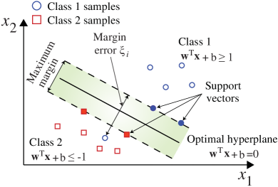
(a)                                                (b)

Figure 2.7: Principle of SVM. (a) The support vector machine (SVM) classifier aims to maximize the margin between the Class 1 and Class 2 training measurements. (b) Semi-supervised learning – exploits both labeled and unlabeled data.

The two differences between the soft-margin SVM and the least squares SVM are: 1) the inequality constraints in (2.56) are replaced by equality constraints in (2.57); and 2) the loss $\sum_{m=1}^{M}\xi_{m}(\xi_{m}\geq 0)$ is replaced by a squared loss. These two modifications enable the solution of the least-squares SVM to be more conveniently obtained, compared to the soft-margin SVM.

Remark 4: According to the statistical learning theory [Vapnik and Vapnik, 1998], SVM-based learning performs well when the number of training measurements is larger than the complexity of the model. Moreover, the complexity of the model and the number of parameters to describe the model are always in a direct proportion.

2.9.2 Support Matrix Machines (SMM)

Recall that the general SVM problem in (2.56) deals with data expressed in a vector form, $\mathbf{x}$. If, on the other hand, the data are collected as matrices, $\mathbf{X}$, these are typically first vectorized by $\text{vec}(\mathbf{X})$, and then fed to the SVM. However, in many classification problems, such as EEG classification, data is naturally expressed by matrices, the structure information could be exploited for a better solution. For matrices, we have $\langle\mathbf{W},\mathbf{W}\rangle=\text{tr}(\mathbf{W}^{\text{T}}\mathbf{W})$, and so intuitively we could consider the following formulation for the soft margin support matrix machine [Luo et al., 2015a]

$$\min_{\mathbf{W},b,\boldsymbol{\xi}}\,\frac{1}{2}\text{tr}(\mathbf{W}^{\text{T}}\mathbf{W})+C\sum_{m=1}^{M}\xi_{m}$$ (2.58)

s.t. $$\hskip 8.53581pty_{m}(\text{tr}(\mathbf{W}^{\text{T}}\mathbf{X}_{m})+b)\geq 1-\xi_{m},\,\boldsymbol{\xi}\geq 0,\quad m=1,\ldots,M.$$

However, observe that when $\mathbf{w}=\text{vec}(\mathbf{W}^{\text{T}})$ the above formulation is essentially equivalent to (2.56) and does not exploit the correlation between the data channels inherent to a matrix structure, since

$$\text{tr}(\mathbf{W}^{\text{T}}\mathbf{X}_{m}) =\text{vec}(\mathbf{W}^{\text{T}})^{\text{T}}\text{vec}(\mathbf{X}_{m}^{\text{T}})=\mathbf{w}^{\text{T}}\mathbf{x}_{m},$$ (2.59)

$$\text{tr}(\mathbf{W}^{\text{T}}\mathbf{W}) =\text{vec}(\mathbf{W}^{\text{T}})^{\text{T}}\text{vec}(\mathbf{W}^{\text{T}})=\mathbf{w}^{\text{T}}\mathbf{w},$$

In order to include correlations between the rows or columns of data matrices, $\mathbf{X}_{m}$, the nuclear norm can be introduced so that the problem becomes

$$\text{arg}\underset{\mathbf{W},b,\xi_{m}}{\text{min}}\ \frac{1}{2}\text{tr}(\mathbf{W}^{\text{T}}\mathbf{W})+\tau\|\mathbf{W}\|_{*}+C\sum_{m=1}^{m}\xi_{m}$$ (2.60)

$$\text{s.t.}\hskip 8.53581pty_{m}(\text{tr}(\mathbf{W}^{\text{T}}\mathbf{X}_{m})+b)\geq 1-\xi_{m}.$$

Note that this is a generalization of the standard SVM, which is obtained for $\tau=0$. The solution to (2.60) is obtained as

$$\tilde{\mathbf{W}}=D_{\tau}\left(\sum_{m=1}^{M}\tilde{\beta}_{m}y_{m}\mathbf{X}_{m}\right),$$ (2.61)

where $D_{\tau}(\mathbf{\cdot})$ is the singular value thresholding operator, which suppresses singular values below $\tau$ to zeros. Denote by $\mathbf{\Omega}=\sum_{m=1}^{M}\tilde{\beta}_{m}y_{m}\mathbf{X}_{m}$ a combination of $\mathbf{X}_{m}$ associated to non-zero ${\tilde{\beta}_{m}}$, which are the so called support matrices [Luo et al., 2015a].

The solution to (2.60) can be obtained by rewriting the problem as

$$\text{arg}\underset{\mathbf{W},b}{\text{min}}\ \frac{1}{2}\text{tr}(\mathbf{W}^{\text{T}}\mathbf{W})+\tau\|\mathbf{W}\|_{*}+C\sum_{m=1}^{M}[1-y_{m}(\text{tr}(\mathbf{W}^{\text{T}}\mathbf{X}_{m})+b)]_{+},$$ (2.62)

which is equivalent to

$$\text{arg}\underset{\mathbf{W},b,\mathbf{S}}{\text{min}}\;H(\mathbf{W},b)+G(\mathbf{S})\quad\text{s.t.}\hskip 11.38109pt\mathbf{S}-\mathbf{W}=\mathbf{0},$$ (2.63)

and

$$H(\mathbf{W},b)=\frac{1}{2}\text{tr}(\mathbf{W}^{\text{T}} \mathbf{W})+C\sum_{m=1}^{M}[1-y_{m}(\text{tr}(\mathbf{W}^{\text{T}}\mathbf{X}_{m})+b)]_{+}$$ (2.64)

$$G(\mathbf{S})=\tau\|\mathbf{S}\|_{*},$$

where $[x]_{+}=\max\{x,0\}$. The solution is obtained using an augmented Lagrangian form

$$L(\mathbf{W},b,\mathbf{S},\mathbf{\Lambda})=H(\mathbf{W},b)+G(\mathbf{S})+\text{tr}(\mathbf{\Lambda}^{\text{T}}(\mathbf{S-W}))+\frac{\rho}{2}\|\mathbf{S-W}\|_{F}^{2},$$ (2.65)

where $\rho>0$ is a hyperparameter.

2.9.3 Support Tensor Machines (STM)

Consider now a typical problem in computer vision, where the objects are represented by data tensors and the number of the training measurement is limited. This naturally leads to a tensor extension of SVM, called the support tensor machine (STM). Consider a general supervised learning scenario with $M$ training measurements, $\{\underline{\mathbf{X}}_{m},y_{m}\},m=1,\ldots,M$, represented by $N$th-order tensors, $\underline{\mathbf{X}}_{m}\in\mathbb{R}^{I_{1}\times I_{2}\times\cdots\times I_{N}}$, which are associated with the scalar variable $y_{m}$. There are two possible scenarios: 1) $y_{m}$ takes a continuous set of values, which leads to the tensor regression problem, and 2) $y_{m}\in\{+1,-1\}$ that is, it takes categorical values, which is a standard classification problem. For the classification case, STM [Tao et al., 2005, Biswas and Milanfar, 2016, Hao et al., 2013] can be formulated through the following minimization problem

$$\begin{split}&\min_{\mathbf{w}_{n},b,\boldsymbol{\xi}}\;J(\mathbf{w}_{n},b,\boldsymbol{\xi})=\frac{1}{2}\left\|\otimes_{n=1}^{N}\mathbf{w}_{n}\right\|^{2}+C\sum_{m=1}^{M}\xi_{m}\\ \mbox{s.t.}&\quad y_{m}\left(\underline{\mathbf{X}}_{m}\bar{\times}_{1}\mathbf{w}_{1}\cdots\bar{\times}_{N}\mathbf{w}_{N}+b\right)\geq 1-\xi_{m},\quad\boldsymbol{\xi}\geq 0,\\ &\quad m=1,\ldots,M.\end{split}$$ (2.66)

Here, $\boldsymbol{\xi}=[\xi_{1},\xi_{2},\ldots,\xi_{M}]^{\text{T}}\in\mathbb{R}^{M}$ is the vector of all slack variables which helps to deal with linearly nonseparable problems.

The STM problem is therefore composed of $N$ quadratic programming (QP)sub-problems with inequality constraints, where the $n$th QP sub-problem can be formulated, as follows [Hao et al., 2013]:

$$\begin{split}&\min_{\mathbf{w}_{n},b,\boldsymbol{\xi}}\;\frac{1}{2}\;\|\mathbf{w}_{n}\|^{2}\,\prod_{1\leq i\leq N}^{i\neq n}(\|\mathbf{w}_{i}\|^{2})+C\sum_{m=1}^{M}\xi_{m}\\ \mbox{s.t.}&\quad y_{m}\left(\mathbf{w}_{n}^{\text{T}}\left(\underline{\mathbf{X}}_{m}{\bar{\times}}_{i\neq n}{{\bf w}_{i}}\right)+b\right)\geq 1-\xi_{m},\quad\boldsymbol{\xi}\geq 0,\\ &m=1,\ldots,M.\end{split}$$ (2.67)

Based on the least squares SVM in (2.57), its tensor extension, referred to as the least squares STM (LS-STM), can be formulated as

$$\begin{split}&\min_{\mathbf{w}_{n},b,\boldsymbol{\varepsilon}}\;J(\mathbf{w}_{n},b,\boldsymbol{\varepsilon})=\frac{1}{2}\left\|{\bf w}_{1}\otimes{\bf w}_{2}\otimes\cdots\otimes{\bf w}_{N}\right\|^{2}+\frac{\gamma}{2}\boldsymbol{\varepsilon}^{\text{T}}\boldsymbol{\varepsilon}\\ \mbox{s.t.}&\quad y_{m}\left(\underline{\mathbf{X}}_{m}\bar{\times}_{1}\mathbf{w}_{1}\cdots\bar{\times}_{N}\mathbf{w}_{N}+b\right)=1-\varepsilon_{m},\quad m=1,\ldots,M.\end{split}$$ (2.68)

Then, the LS-STM solution can be obtained by the following alternating least squares optimization problem (see Algorithm 6)

$$\begin{split}&\min_{\mathbf{w}_{n},b,\boldsymbol{\varepsilon}}\;\frac{1}{2}\;\|\mathbf{w}_{n}\|^{2}\;\prod_{1\leq i\leq N}^{i\neq n}(\|\mathbf{w}_{i}\|^{2})\;+\frac{\gamma}{2}\boldsymbol{\varepsilon}^{\text{T}}\boldsymbol{\varepsilon}\\ \mbox{s.t.}&\quad y_{m}\left(\mathbf{w}_{n}^{\text{T}}\left(\underline{\mathbf{X}}_{m}{\bar{\times}}_{i\neq n}{\bf w}_{i}\right)+b\right)=1-\varepsilon_{m},\quad m=1,\ldots,M.\end{split}$$ (2.69)

Once the STM solution has been obtained, the class label of a test example, $\underline{\mathbf{X}}_{*}$, can be predicted by a nonlinear transformation

$$y(\underline{\mathbf{X}})=\text{sign}\left(\underline{\mathbf{X}}_{*}\bar{\times}_{1}\mathbf{w}_{1}\cdots\bar{\times}_{N}\mathbf{w}_{N}+b\right).$$ (2.70)

0:  $\{\underline{\mathbf{X}}_{m},y_{m}\},m=1,\ldots,M$ where $\underline{\mathbf{X}}_{m}\in\mathbb{R}^{I_{1}\times I_{2}\times\cdots\times I_{N}}$, $y_{m}\in\{+1,-1\}$ and the penalty coefficient $\gamma$. 0:  $\{\mathbf{w}_{n}\},n=1,\ldots,N$ and $b$. 1:  Initialization: Random vectors $\{\mathbf{w}_{n}\},n=1,\ldots,N$. 2:  while not converged or iteration limit is not reached do 3:     for $n=1$ to $N$ do 4:        $\eta\leftarrow\prod_{1\leq i\leq N}^{i\neq n}\|\mathbf{w}_{i}\|^{2}$, 5:        $\mathbf{x}_{m}=\underline{\mathbf{X}}_{m}{\bar{\times}}_{i\neq n}{\bf w}_{i}$ 6:        Compute $\mathbf{w}_{n}$ by solving the optimization problem $\displaystyle\min_{\mathbf{w}_{n},b,\boldsymbol{\varepsilon}}\,\frac{\eta}{2}\|\mathbf{w}_{n}\|^{2}+\frac{\gamma}{2}\boldsymbol{\varepsilon}^{\text{T}}\boldsymbol{\varepsilon}$ s.t. $\displaystyle\quad y_{m}\left(\mathbf{w}_{n}^{\text{T}}\mathbf{x}_{m}+b\right)=1-\varepsilon_{m},$ $\displaystyle\quad m=1,\ldots,M.$ 7:     end for 8:  end while

Algorithm 6 Least Squares Support Tensor Machine (LS-STM)

In practice, it is often more convenient to solve the optimization problem (2.67) by considering the dual problem, given by

$$\begin{split}&\max_{\{\alpha_{i}\}_{i=1}^{M}}\sum_{m=1}^{M}\alpha_{m}-\frac{1}{2}\sum_{i,j=1}^{M}\alpha_{i}\alpha_{j}y_{i}y_{j}\langle\underline{\mathbf{X}}_{i},\underline{\mathbf{X}}_{j}\rangle,\\ \mbox{s.t.}&\quad\sum_{m=1}^{M}\alpha_{m}y_{m}=0,\quad 0\leq\alpha_{m}\leq C,\quad m=1,\ldots,M,\end{split}$$ (2.71)

where $\alpha_{m}$ are the Lagrange multipliers and $\langle\underline{\mathbf{X}}_{i},\underline{\mathbf{X}}_{j}\rangle$ the inner products of $\underline{\mathbf{X}}_{i}$ and $\underline{\mathbf{X}}_{j}$.

It is obvious that when the input samples, $\underline{\mathbf{X}}_{i}$, are vectors, this optimization model simplifies into the standard vector SVM. Moreover, if the original input tensors are used to compute $\langle\underline{\mathbf{X}}_{i},\underline{\mathbf{X}}_{j}\rangle$, then the optimal solutions are the same as those produced by the SVM. Consider now the rank-one decompositions of $\underline{\mathbf{X}}_{i}$ and $\underline{\mathbf{X}}_{j}$ in the form $\underline{\mathbf{X}}_{i}\approx\sum_{r=1}^{R}\mathbf{x}_{ir}^{(1)}\circ\mathbf{x}_{ir}^{(2)}\circ\cdots\circ\mathbf{x}_{ir}^{(N)}$ and $\underline{\mathbf{X}}_{j}\approx\sum_{r=1}^{R}\mathbf{x}_{jr}^{(1)}\circ\mathbf{x}_{jr}^{(2)}\circ\cdots\circ\mathbf{x}_{jr}^{(N)}$. Then, the inner product of $\underline{\mathbf{X}}_{i}$ and $\underline{\mathbf{X}}_{j}$ is given by Hao et al. [2013]

$$\langle\underline{\mathbf{X}}_{i},\underline{\mathbf{X}}_{j}\rangle\approx\sum_{p=1}^{R}\sum_{q=1}^{R}\left\langle\mathbf{x}_{ip}^{(1)},\mathbf{x}_{jq}^{(1)}\right\rangle\left\langle\mathbf{x}_{ip}^{(2)},\mathbf{x}_{jq}^{(2)}\right\rangle\cdots\left\langle\mathbf{x}_{ip}^{(N)},\mathbf{x}_{jq}^{(N)}\right\rangle,$$ (2.72)

and (2.71) can be solved by a sequential QP optimization algorithm. The class label of a test example $\underline{\mathbf{X}}_{*}$ is then predicted as

$$y(\underline{\mathbf{X}}_{*})=\text{sign}\left(\sum_{m=1}^{M}\sum_{p=1}^{R}\sum_{q=1}^{R}\alpha_{m}y_{m}\prod_{n=1}^{N}\left\langle\mathbf{x}_{mp}^{(n)},\mathbf{x}_{*q}^{(n)}\right\rangle+b\right).$$ (2.73)

2.10 Higher Rank Support Tensor Machines (HRSTM)

Higher Rank STMs (HRSTM) aim to estimate a set of parameters in the form of the sum of rank-one tensors [Kotsia et al., 2012], which defines a separating hyperplane between classes of data. The benefits of this scheme are twofold:

1. The use of a direct CP representation is intuitively closer to the idea of properly processing tensorial input data, as the data structure is more efficiently retained;

2. The use of simple CP decompositions allows for multiple projections of the input tensor along each mode, leading to considerable improvements in the discriminative ability of the resulting classifier.

The corresponding optimization problems can be solved in an iterative manner utilizing, e.g., the standard CP decomposition, where at each iteration the parameters corresponding to the projections along a single tensor mode are estimated by solving a typical STM-type optimization problem.

The aim of the so formulated STM is therefore to learn a multilinear decision function, $g:\mathbf{R}^{I_{1}\times I_{2}\times\cdots\times I_{N}}\rightarrow[-1,1]$, which classifies a test tensor $\underline{\mathbf{X}}\in\mathbf{R}^{I_{1}\times I_{2}\times\cdots\times I_{N}}$, by using the nonlinear transformation $g(\underline{\mathbf{X}})=\text{sign}(\langle\underline{\mathbf{X}},\underline{\mathbf{W}}\rangle+b)$.

The weight tensor, $\underline{\mathbf{W}}$, is estimated by solving the following soft STMs optimization problem

$$\begin{split}&\min_{\underline{\mathbf{W}},b,\boldsymbol{\xi}}\;\frac{1}{2}\langle\underline{\mathbf{W}},\underline{\mathbf{W}}\rangle+C\sum_{m=1}^{M}\xi_{m},\\ \mbox{s.t.}\quad&y_{m}\left(\langle\underline{\mathbf{W}},\underline{\mathbf{X}}_{m}\rangle+b\right)\geq 1-\xi_{m},\quad\xi_{m}\geq 0,\quad m=1,\ldots,M,\end{split}$$ (2.74)

where $b$ is the bias term, $\boldsymbol{\xi}=[\xi_{1},\ldots,\xi_{m}]^{\text{T}}$ is the vector of slack variables and $C$ is the term which controls the relative importance of penalizing the training errors. The training is performed in such a way that the margin of the support tensors is maximized while the upper bound on the misclassification errors in the training set is minimized.

Consider, as an example, the case where the weight parameter, $\underline{\mathbf{W}}$, is represented via a CP model, to give

$$\underline{\mathbf{W}}=\sum_{r=1}^{R}\mathbf{u}_{r}^{(1)}\circ\mathbf{u}_{r}^{(2)}\circ\cdots\circ\mathbf{u}_{r}^{(N)},$$ (2.75)

where $\mathbf{u}_{r}^{(n)}\in\mathbb{R}^{I_{n}},\;\;n=1,2,\ldots,N$. Then, the $n$-th mode matricization of $\underline{\mathbf{W}}$ can be written as

$$\mathbf{W}_{(n)}=\mathbf{U}^{(n)}(\mathbf{U}^{(N)}\odot\cdots\odot\mathbf{U}^{(n+1)}\odot\mathbf{U}^{(n-1)}\odot\cdots\odot\mathbf{U}^{(1)})^{\text{T}}=\mathbf{U}^{(n)}(\mathbf{U}^{(-n)})^{\text{T}},$$ (2.76)

where $\odot$ denotes the Khatri-Rao product. Note that the inner product in (2.74) can be computed very efficiently e.g., in the form

$$\langle\underline{\mathbf{W}},\underline{\mathbf{W}}\rangle=\mathop{\rm tr}\nolimits[\mathbf{W}_{(n)}\mathbf{W}_{(n)}^{\text{T}}]=\text{vec}(\mathbf{W}_{(n)})^{\text{T}}\text{vec}(\mathbf{W}_{(n)}).$$ (2.77)

The above optimization problem, however, is not convex with respect to all sets of parameters in $\underline{\mathbf{W}}$. For this reason, we adopt an iterative scheme in which at each iteration we solve only for the parameters that are associated with the $n$-th mode of the parameter tensor $\underline{\mathbf{W}}$, while keeping all the other parameters fixed, similarly to the ALS algorithm. More specifically, for the $n$-th mode, at each iteration we solve the following optimization problem

$$\begin{split}&\min_{\mathbf{W}_{(n)},b,\boldsymbol{\xi}}\,\frac{1}{2}\mathop{\rm tr}\nolimits\left(\mathbf{W}_{(n)}\mathbf{W}_{(n)}^{\text{T}}\right)+C\sum_{m=1}^{M}\xi_{m},\\ \mbox{s.t.}\quad&y_{m}\left(\mathop{\rm tr}\nolimits\left(\mathbf{W}_{(n)}\mathbf{X}_{m(n)}^{\text{T}}\right)+b\right)\geq 1-\xi_{m},\quad\xi_{m}\geq 0,\\ &\quad m=1,\ldots,M,\quad n=1,\ldots,N,\end{split}$$ (2.78)

Under the assumption that the tensor $\underline{\mathbf{W}}$ is represented as a sum of rank one tensors, we can replace the above matrices by $\mathbf{W}_{(n)}=\mathbf{U}^{(n)}(\mathbf{U}^{(-n)})^{\text{T}}$, and thus the above equation becomes

$$\begin{split}&\min_{\mathbf{U}^{(n)},b,\boldsymbol{\xi}}\,\frac{1}{2}\mathop{\rm tr}\nolimits(\mathbf{U}^{(n)}(\mathbf{U}^{(-n)})^{\text{T}}(\mathbf{U}^{(-n)})(\mathbf{U}^{(n)})^{\text{T}})+C\sum_{m=1}^{M}\xi_{m},\\ \mbox{s.t.}\quad&y_{m}\left(\mathop{\rm tr}\nolimits\left(\mathbf{U}^{(n)}(\mathbf{U}^{(-n)})^{\text{T}}\mathbf{X}^{\text{T}}_{m(n)}\right)+b\right)\geq 1-\xi_{m},\quad\xi_{m}\geq 0,\\ &\quad m=1,\ldots,M,\quad n=1,\ldots,N.\end{split}$$ (2.79)

At each iteration the optimization problem is solved for only one set of matrices $\mathbf{U}^{(n)}$ for the mode $n$, while keeping the other matrices $\mathbf{U}^{(k)}$ for $k\neq n$, fixed. Note that the optimization problem defined in (2.79) can also be solved using a classic vector-based SVM implementation.

Let us define $\mathbf{A}=\mathbf{U}^{(-n)^{\text{T}}}\mathbf{U}^{(-n)}$, which is a positive definite matrix, and let $\widetilde{\mathbf{U}}^{(n)}=\mathbf{U}^{(n)}\mathbf{A}^{\frac{1}{2}}$. Then,

$$\begin{split}\mathop{\rm tr}\nolimits[\mathbf{U}^{(n)}(\mathbf{U}^{(-n)})^{\text{T}}(\mathbf{U}^{(-n)})(\mathbf{U}^{(n)})^{\text{T}}]&=\mathop{\rm tr}\nolimits[\widetilde{\mathbf{U}}^{(n)}(\widetilde{\mathbf{U}}^{(n)})^{\text{T}}]\\ &=\text{vec}(\widetilde{\mathbf{U}}^{(n)})^{\text{T}}\text{vec}(\widetilde{\mathbf{U}}^{(n)}).\end{split}$$ (2.80)

By letting $\widetilde{\mathbf{X}}_{m(n)}=\mathbf{X}_{m(n)}\mathbf{U}^{(-n)}\mathbf{A}^{-\frac{1}{2}}$, we have

$$\begin{split}\mathop{\rm tr}\nolimits[\mathbf{U}^{(n)}(\mathbf{U}^{(-n)})^{\text{T}}\mathbf{X}_{m(n)}^{\text{T}}]&=\mathop{\rm tr}\nolimits[\widetilde{\mathbf{U}}^{(n)}\widetilde{\mathbf{X}}^{\text{T}}_{m(n)}]\\ &=\text{vec}(\widetilde{\mathbf{U}}^{(n)})^{\text{T}}\text{vec}(\widetilde{\mathbf{X}}_{m(n)}).\end{split}$$ (2.81)

Then, the optimization problem (2.79) can be simplified as

$$\begin{split}&\min_{\mathbf{U}^{(n)},b,\boldsymbol{\xi}}\,\frac{1}{2}\text{vec}(\widetilde{\mathbf{U}}^{(n)})^{\text{T}}\text{vec}(\widetilde{\mathbf{U}}^{(n)})+C\sum_{m=1}^{M}\xi_{m},\\ \mbox{s.t.}\quad&y_{m}\left(\text{vec}(\widetilde{\mathbf{U}}^{(n)})^{\text{T}}\text{vec}(\widetilde{\mathbf{X}}_{m(n)})+b\right)\geq 1-\xi_{m},\quad\xi_{m}\geq 0,\\ &\quad m=1,\ldots,M,\quad n=1,\ldots,N.\end{split}$$ (2.82)

Observe that now the STM optimization problem for the $n$-th mode in (2.79) can be formulated as a standard vector SVM problem with respect to $\widetilde{\mathbf{U}}^{(n)}$. In other words, such a procedure leads to a straightforward implementation of the algorithm by solving (2.82) with respect to $\widetilde{\mathbf{U}}^{(n)}$ using a standard SVM implementation, and then solving for $\mathbf{U}^{(n)}$ as $\mathbf{U}^{(n)}=\widetilde{\mathbf{U}}^{(n)}\mathbf{A}^{-\frac{1}{2}}$.

2.11 Kernel Support Tensor Machines

The class of support tensor machines has been recently extended to the nonlinear case by using the kernel framework, and is referred to as kernel support tensor regression (KSTR) [Gao and Wu, 2012]. After mapping each row of every original tensor (or every tensor converted from original vector) onto a high-dimensional space, we obtain the associated points in a new high-dimensional feature space, and then compute the regression function. Suppose we are given a set of training samples $\{\underline{\mathbf{X}}_{m},y_{m}\},m=1,\ldots,M$, where each training sample, $\underline{\mathbf{X}}_{m}$, is a data point in $\mathbb{R}^{I_{1}}\otimes\mathbb{R}^{I_{2}}$, where $\mathbb{R}^{I_{1}}$ and $\mathbb{R}^{I_{2}}$ are two vector spaces, and $y_{m}$ is the target value associated with $\underline{\mathbf{X}}_{m}$. Denote by ${\bf z}_{mp}$ the $p$-th row of $\underline{\mathbf{X}}_{m}$, we can then use a nonlinear mapping function $\varphi(\underline{\mathbf{X}}_{m})$ to map $\underline{\mathbf{X}}_{m}$ onto a high-dimensional tensor feature space, and define a nonlinear mapping function for tensor $\underline{\mathbf{X}}_{m}$, given by

$$\phi(\underline{\mathbf{X}}_{m})=\left[\begin{array}[]{c}\varphi({\bf z}_{m1})\\ \varphi({\bf z}_{m2})\\ \vdots\\ \varphi({\bf z}_{mI_{1}})\end{array}\right].$$ (2.83)

In this way, we can obtain the new kernel function

$$\begin{split}K(\underline{\mathbf{X}}_{m},\underline{\mathbf{X}}_{n})&=\phi(\underline{\mathbf{X}}_{m})\phi(\underline{\mathbf{X}}_{n})^{\text{T}}=\left[\begin{array}[]{c}\varphi({\bf z}_{m1})\\ \varphi({\bf z}_{m2})\\ \vdots\\ \varphi({\bf z}_{mI_{1}})\end{array}\right]\left[\begin{array}[]{c}\varphi({\bf z}_{n1})\\ \varphi({\bf z}_{n2})\\ \vdots\\ \varphi({\bf z}_{nI_{1}})\end{array}\right]^{\text{T}}\\ &=\left[\begin{array}[]{ccc}\varphi({\bf z}_{m1})\varphi({\bf z}_{n1})^{\text{T}}&\cdots&\varphi({\bf z}_{m1})\varphi({\bf z}_{nI_{1}})^{\text{T}}\\ \vdots&\ddots&\vdots\\ \varphi({\bf z}_{mI_{1}})\varphi({\bf z}_{n1})^{\text{T}}&\cdots&\varphi({\bf z}_{mI_{1}})\varphi({\bf z}_{nI_{1}})^{\text{T}}\\ \end{array}\right].\end{split}$$ (2.84)

Note that such a kernel function is quite different from the function used in the SVR - the output of this kernel function is a matrix as opposed to a scalar in SVR.

For instance, if we use an RBF kernel function within KSTR, then the $mn$-th element of the kernel matrix is expressed as

$$\varphi({\bf z}_{mp_{1}})\varphi({\bf z}_{np_{2}})^{\text{T}}=e^{-\gamma\|{\bf z}_{mp_{1}}-{\bf z}_{np_{2}}\|^{2}}.$$ (2.85)

The support tensor regression with an $\varepsilon$-insensitive loss function is similar to standard support tensor regression, and the regression function in such a case can be defined as

$$f(\underline{\mathbf{X}})=\mathbf{u}^{\text{T}}\phi(\underline{\mathbf{X}})\mathbf{v}+b.$$ (2.86)

This function can be estimated by solving the following quadratic programming problem

$$\begin{split}&\min_{\mathbf{u,v},b,\xi_{m},\xi_{m}^{*}}\,\frac{1}{2}\left\|\mathbf{uv}^{\text{T}}\right\|^{2}+C\sum_{m=1}^{M}(\xi_{m}+\xi_{m}^{*})\\ \mbox{s.t.}\quad&\left\{\begin{array}[]{ll}y_{m}-\mathbf{u}^{\text{T}}\phi(\underline{\mathbf{X}}_{m})\mathbf{v}-b&\leq\varepsilon-\xi_{m},\\ \mathbf{u}^{\text{T}}\phi(\underline{\mathbf{X}}_{m})\mathbf{v}+b-y_{m}&\leq\varepsilon+\xi_{m}^{*},\quad m=1,\ldots,M,\\ \xi_{m},\xi_{m}^{*}&\geq 0,\end{array}\right.\end{split}$$ (2.87)

where $C$ is a pre-specified constant, $\varepsilon$ is a user-defined scalar, and $\xi_{m},\xi_{m}^{*}$ are slack variables which represent the upper and lower constraints on the outputs of the classification system.

Consider again (2.87), and let $\mathbf{u}$ be a column vector of the same dimension as the row number of samples; we can then calculate the vector $\mathbf{v}$ using the Lagrange multiplier method, where the Lagrangian is constructed according to

$$\begin{split}\max_{\alpha_{m},\alpha_{m}^{*},\eta_{m},\eta_{m}^{*}}\min_{\mathbf{v},b,\xi_{m},\xi_{m}^{*}}&\left\{\begin{array}[]{l}L=\frac{1}{2}\|\mathbf{u}\mathbf{v}^{\text{T}}\|^{2}+C\sum_{m=1}^{M}(\xi_{m}+\xi_{m}^{*})\\ -\sum_{m=1}^{M}(\eta_{m}\xi_{m}+\eta_{m}^{*}\xi_{m}^{*})-\\ \sum_{m=1}^{M}\alpha_{m}(\varepsilon+\xi_{m}-y_{m}+\mathbf{u}^{\text{T}}\phi(\underline{\mathbf{X}}_{m})\mathbf{v}+b)\\ -\sum_{m=1}^{M}\alpha_{m}^{*}(\varepsilon+\xi_{m}^{*}-y_{m}+\mathbf{u}^{\text{T}}\phi(\underline{\mathbf{X}}_{m})\mathbf{v}+b)\end{array}\right\}\\ \mbox{s.t.}\quad&\alpha_{m},\alpha_{m}^{*},\eta_{m},\eta_{m}^{*}\geq 0,\quad m=1,\ldots,M,\end{split}$$ (2.88)

and $\alpha_{m},\alpha_{m}^{*},\eta_{m},\eta_{m}^{*}$ are the Lagrange multipliers. In next step, we determine the Lagrange multipliers $\alpha_{m},\alpha_{m}^{*}$ and $\mathbf{v}$, $\|\mathbf{v}\|^{2}$.

Alternatively, let $\mathbf{x}_{n}^{\prime}=\mathbf{v}^{\text{T}}\phi(\underline{\mathbf{X}}_{n})=\frac{1}{\|\mathbf{u}\|^{4}}\sum_{m=1}^{M}(\alpha_{m}-\alpha_{m}^{*})K(\underline{\mathbf{X}}_{m},\underline{\mathbf{X}}_{n})$ be the new training samples. Then, we construct another Lagrangian

$$\begin{split}\max_{\alpha_{m},\alpha_{m}^{*},\eta_{m},\eta_{m}^{*}}\min_{\mathbf{u},b,\xi_{m},\xi_{m}^{*}}&\left\{\begin{array}[]{l}L=\frac{1}{2}\|\mathbf{uv}^{\text{T}}\|^{2}+C\sum_{m=1}^{M}(\xi_{m}+\xi_{m}^{*})\\ -\sum_{m=1}^{M}(\eta_{m}\xi_{m}+\eta_{m}^{*}\xi_{m}^{*})-\\ \sum_{m=1}^{M}\alpha_{m}(\varepsilon+\xi_{m}-y_{m}+\mathbf{x}^{\prime}_{m}\mathbf{u}+b)\\ -\sum_{m=1}^{M}(\alpha_{m}^{*}(\varepsilon+\xi_{m}^{*}+y_{m}-\mathbf{x}^{\prime}_{m}\mathbf{u}-b))\end{array}\right\}\\ \mbox{s.t.}\quad&\alpha_{m},\alpha_{m}^{*},\eta_{m},\eta_{m}^{*}\geq 0,\quad m=1,\ldots,M,\end{split}$$ (2.89)

and obtain $\mathbf{u}$ and $b$. These two steps are performed iteratively to compute $\mathbf{v,u},b$.

The KSTR method has the following advantages over the STR method: i) it has a strong ability to learn and a superior generalization ability; ii) the KSTR is able to solve nonlinearly separable problems more efficiently. A disadvantage of KSTR is that the computational load of KSTR is much higher than that of STR.

2.12 Tensor Fisher Discriminant Analysis (FDA)

Fisher discriminant analysis (FDA) has been widely applied for classification. It aims to find a direction which separates the class means well while minimizing the variance of the total training measurements. This procedure is equivalent to maximizing the symmetric Kullback-Leibler divergence (KLD) between positive and negative measurements with identical covariances, so that the positive measurements are separated from the negative measurements. To extend the FDA to tensors, that is, to introduce Tensor FDA (TFDA), consider $M$ training measurements, $\underline{\mathbf{X}}_{m}\in\mathbb{R}^{I_{1}\times I_{2}\times\cdots\times I_{N}},\;\;m=1,\ldots,M$, associated with the class labels $y_{m}\in\{+1,-1\}$. The mean of positive training measurements is $\underline{\mathbf{L}}_{+}=(1/M_{+})\sum_{m=1}^{M}({I}(y_{m}=+1)\underline{\mathbf{X}}_{m})$, the mean of the negative training measurements is $\underline{\mathbf{L}}_{-}=(1/M_{-})\sum_{m=1}^{M}({I}(y_{m}=-1)\underline{\mathbf{X}}_{m})$, the mean of all training measurements is $\underline{\mathbf{L}}=(1/M)\sum_{m=1}^{M}\underline{\mathbf{X}}_{m}$, and $M_{+}(M_{-})$ are the numbers of the positive (negative) measurements. The decision function is a multilinear function $y(\underline{\mathbf{X}})=\text{sign}(\underline{\mathbf{X}}\bar{\times}_{1}\mathbf{w}_{1}\cdots\bar{\times}_{N}\mathbf{w}_{N}+b)$, while the projection vectors, $\mathbf{w}_{n}\in\mathbb{R}^{I_{n}},\;n=1,\ldots,N$, and the bias $b$ in TFDA are obtained from

$$\max_{\mathbf{w}_{n}|_{n=1}^{N}}\,J(\mathbf{w}_{n})=\frac{\|(\underline{\mathbf{L}}_{+}-\underline{\mathbf{L}}_{-})\bar{\times}_{1}\mathbf{w}_{1}\cdots\bar{\times}\mathbf{w}_{N}\|^{2}}{\sum_{m=1}^{M}\|(\underline{\mathbf{X}}_{m}-\underline{\mathbf{L}})\bar{\times}_{1}\mathbf{w}_{1}\cdots\bar{\times}\mathbf{w}_{N}\|^{2}}.$$ (2.90)

Unfortunately, there is no closed-form solution for TFDA, however, alternating projection algorithms can be applied to iteratively obtain the desired solution using the TFDA framework. For the projection vectors $\mathbf{w}_{n}|_{n=1}^{N}$, we can obtain the bias $b$ using

$$b=\frac{M_{-}-M_{+}-(M_{+}\underline{\mathbf{L}}_{+}+M_{-}\underline{\mathbf{L}}_{-})\bar{\times}_{1}\mathbf{w}_{1}\cdots\bar{\times}_{N}\mathbf{w}_{N}}{M_{-}+M_{+}}.$$ (2.91)

The regularized Multiway Fisher Discriminant Analysis (MFDA) [Lechuga et al., 2015] aims to impose the structural constraints in such a way that the weight vector $\mathbf{w}$ will be decomposed as $\mathbf{w}=\mathbf{w}_{N}\otimes\cdots\otimes\mathbf{w}_{1}$. Let $\mathbf{X}_{(1)}\in\mathbb{R}^{M\times I_{1}I_{2}\cdots I_{N}}$ be an unfolded matrix of observed samples and $\mathbf{Y}\in\mathbb{R}^{M\times C}$ the matrix of dummy variables indicating the group memberships. The optimization problem of MFDA can then be formulated as

$$\begin{split}\arg&\max_{\mathbf{w}}\frac{\mathbf{w}^{\text{T}}\mathbf{S}_{B}\mathbf{w}}{\mathbf{w}^{\text{T}}\mathbf{S}_{T}\mathbf{w}+\lambda\mathbf{w}^{\text{T}}\mathbf{R}\mathbf{w}}\\ \end{split}$$ (2.92)

where $\mathbf{w}$ denotes $\mathbf{w}_{N}\otimes\cdots\otimes\mathbf{w}_{1}$, $\mathbf{S}_{B}=\mathbf{X}_{(1)}^{\text{T}}\mathbf{Y}(\mathbf{Y}^{\text{T}}\mathbf{Y})^{-1}\mathbf{Y}^{\text{T}}\mathbf{X}_{(1)}$ is the between covariance matrix, $\mathbf{S}_{T}=\mathbf{X}_{(1)}^{\text{T}}\mathbf{X}_{(1)}$ is the total covariance matrix, and $\mathbf{R}$ is usually an identity matrix. The regularization term $\lambda\mathbf{w}^{\text{T}}\mathbf{R}\mathbf{w}$ is added to improve the numerical stability when computing the inverse of $\mathbf{S}_{T}$ in high-dimensional settings $(M\ll I_{1}I_{2}\cdots I_{N})$. This optimization problem can be solved in an alternate fashion by fixing all $\mathbf{w}_{n}$ except one.

The Linear Discriminant Analysis (LDA) can also be extended to tensor data, which is referred to as Higher Order Discriminant Analysis (HODA) [Phan and Cichocki, 2010] and Multilinear Discriminant Analysis (MDA) [Li and Schonfeld, 2014]. Suppose that we have $M$ tensor samples $\underline{\mathbf{X}}_{m}\in\mathbb{R}^{I_{1}\times I_{2}\times\cdots\times I_{N}},m=1,\ldots,M$ belonging to one of the $C$ classes, and $M_{c}$ is the number of samples in class $c$ such that $M=\sum_{c=1}^{C}M_{c}$. $y_{m}$ denotes the associated class label of $\underline{\mathbf{X}}_{m}$. The class mean tensor for class $c$ is computed by $\underline{\mathbf{L}}_{c}=\frac{1}{M_{c}}\sum_{m=1}^{M_{c}}\underline{\mathbf{X}}_{m}I(y_{m}=c)$, and the total mean tensor is $\underline{\mathbf{L}}=\frac{1}{M}\sum_{m=1}^{M}\underline{\mathbf{X}}_{m}$. The goal is to find the set of optimal projection matrices $\mathbf{W}_{1},\mathbf{W}_{2},\ldots,\mathbf{W}_{N}$ ($\mathbf{W}_{n}\in\mathbb{R}^{I_{n}\times J_{n}}$ for $n=1,\ldots,N$) that lead to the most accurate classification in the projected tensor subspace where

$$\underline{\mathbf{Z}}_{m}=\underline{\mathbf{X}}_{m}\times_{1}\mathbf{W}_{1}^{\text{T}}\cdots\times_{N}\mathbf{W}_{N}^{\text{T}}\in\mathbb{R}^{J_{1}\times J_{2}\times\cdots\times J_{N}}.$$ (2.93)

The mean tensor of class $c$ in the projected subspace is given by

$$\widetilde{\underline{\mathbf{L}}}_{c}=\frac{1}{M_{c}}\sum_{m=1}^{M_{c}}\underline{\mathbf{Z}}_{m}I(y_{m}=c)=\underline{\mathbf{L}}_{c}\times_{1}\mathbf{W}_{1}^{\text{T}}\cdots\times_{N}\mathbf{W}_{N}^{\text{T}},$$ (2.94)

which is simply the projection of $\underline{\mathbf{L}}_{c}$. Similarly, the total mean tensor of projected samples is $\underline{\mathbf{L}}\times_{1}\mathbf{W}_{1}^{\text{T}}\cdots\times_{N}\mathbf{W}_{N}^{\text{T}}$.

The mode-$n$ between-class scatter matrix in the projected tensor subspace can be derived, as follows

$$\begin{split}\mathbf{B}_{n}=&\sum_{c=1}^{C}M_{c}\left[\left(\underline{\mathbf{L}}_{c}\prod_{n=1}^{N}\times_{n}\mathbf{W}_{n}^{\text{T}}\right)_{(n)}-\left(\underline{\mathbf{L}}\prod_{n=1}^{N}\times_{n}\mathbf{W}_{n}^{\text{T}}\right)_{(n)}\right]\\ &\left[\left(\underline{\mathbf{L}}_{c}\prod_{n=1}^{N}\times_{n}\mathbf{W}_{n}^{\text{T}}\right)_{(n)}-\left(\underline{\mathbf{L}}\prod_{n=1}^{N}\times_{n}\mathbf{W}_{n}^{\text{T}}\right)_{(n)}\right]^{\text{T}}\\ =&\mathbf{W}_{n}^{\text{T}}\left\{\sum_{c=1}^{C}M_{c}\left[(\underline{\mathbf{L}}_{c}-\underline{\mathbf{L}})\prod_{k=1,k\neq n}^{N}\times_{k}\mathbf{W}_{n}^{\text{T}}\right]_{(n)}\right.\\ &\left.\left[(\underline{\mathbf{L}}_{c}-\underline{\mathbf{L}})\prod_{k=1,k\neq n}^{N}\times_{k}\mathbf{W}_{n}^{\text{T}}\right]_{(n)}^{\text{T}}\right\}\mathbf{W}_{n}\\ =&\mathbf{W}_{n}^{\text{T}}\mathbf{B}_{-n}\mathbf{W}_{n}.\end{split}$$ (2.95)

Note that $\underline{\mathbf{L}}\prod_{n=1}^{N}\times_{n}{\bf W}_{n}^{\text{T}}=\underline{\mathbf{L}}\times_{1}{\bf W}_{1}^{\text{T}}\times_{2}{\bf W}_{2}^{\text{T}}\cdots\times_{N}{\bf W}_{N}^{\text{T}}$. Here, $\mathbf{B}_{-n}$ denotes the mode-$n$ between-class scatter matrix in the partially projected tensor subspace (by all tensor modes except for mode $n$). The mode-$n$ between class scatter matrix characterizes the separation between $C$ classes in terms of mode-$n$ unfolding of the tensor samples.

Similarly, the mode-$n$ within-class scatter matrix is

$$\begin{split}\mathbf{S}_{n}=&\mathbf{W}_{n}^{\text{T}}\left\{\sum_{c=1}^{C}\sum_{m=1}^{M_{c}}\left[(\underline{\mathbf{X}}_{m}^{c}-\underline{\mathbf{L}}_{c})\prod_{k=1,k\neq n}^{N}\times_{k}\mathbf{W}_{k}^{\text{T}}\right]_{(n)}\right.\\ &\left.\left[(\underline{\mathbf{X}}_{m}^{c}-\underline{\mathbf{L}}_{c})\prod_{k=1,k\neq n}^{N}\times_{k}\mathbf{W}_{k}^{\text{T}}\right]_{(n)}^{\text{T}}\right\}\mathbf{W}_{n}\\ =&\mathbf{W}_{n}^{\text{T}}\mathbf{S}_{-n}\mathbf{W}_{n},\end{split}$$ (2.96)

where $\mathbf{S}_{-n}$ represents the mode-$n$ within-class scatter matrix in the partially projected tensor subspace (in all tensor modes except for $n$). Finally, the MDA objective function can be described as

$$\begin{split}J(\mathbf{W}_{n})=&\frac{\sum_{c=1}^{C}M_{c}\|(\underline{\mathbf{L}}_{c}-\underline{\mathbf{L}})\prod_{n=1}^{N}\times_{n}\mathbf{W}_{n}^{\text{T}}\|_{F}^{2}}{\sum_{c=1}^{C}\sum_{m=1}^{M_{c}}\|(\underline{\mathbf{X}}_{m}^{c}-L_{c})\prod_{n=1}^{N}\times_{n}\mathbf{W}_{n}^{\text{T}}\|_{F}^{2}}\\ =&\frac{\text{Tr}(\mathbf{W}_{n}^{\text{T}}\mathbf{B}_{-n}\mathbf{W}_{n})}{\text{Tr}(\mathbf{W}_{n}^{\text{T}}\mathbf{S}_{-n}\mathbf{W}_{n})},\end{split}$$ (2.97)

and the set of optimal projection matrices should maximize $J(\mathbf{W}_{n})$ for $n=1,\ldots,N$ simultaneously, to best preserve the given class structure.

In this section, we have discussed SVM and STM for medium and large scale problems. For big data classification problems quite perspective and promising is a quantum computing approach [Rebentrost et al., 2014, Schuld et al., 2015, Li et al., 2015, Chatterjee and Yu, 2016, Biamonte et al., 2016] and a tensor network approach discussed in the next Chapter 3.

Chapter 3 Tensor Train Networks for Selected Huge-Scale Optimization Problems

For extremely large-scale, multidimensional datasets, due to curse of dimensionality, most standard numerical methods for computation and optimization problems are intractable. This chapter introduces feasible solutions for several generic huge-scale dimensionality reduction and related optimization problems, whereby the involved optimized cost functions are approximated by suitable low-rank TT networks. In this way, a very large-scale optimization problem can be converted into a set of much smaller optimization sub-problems of the same kind [Schollwöck, 2011, 2013, Holtz et al., 2012a, Dolgov et al., 2014, Kressner et al., 2014a, Cichocki, 2014, Lee and Cichocki, 2016b], which can be solved using standard methods.

The related optimization problems often involve structured matrices and vectors with over a billion entries (see [Grasedyck et al., 2013, Dolgov, 2014, Garreis and Ulbrich, 2017, Stoudenmire and Schwab, 2016, Hubig et al., 2017] and references therein). In particular, we focus on Symmetric Eigenvalue Decomposition (EVD/PCA) and Generalized Eigenvalue Decomposition (GEVD) [Dolgov et al., 2014, Kressner et al., 2014a, Hubig et al., 2015, Kressner and Uschmajew, 2016, Huckle and Waldherr, 2012, Zhang et al., 2016], SVD [Lee and Cichocki, 2015], solutions of overdetermined and undetermined systems of linear algebraic equations [Oseledets and Dolgov, 2012, Dolgov and Savostyanov, 2014], the Moore–Penrose pseudo-inverse of structured matrices [Lee and Cichocki, 2016b], and LASSO regression problems [Lee and Cichocki, 2016a]. Tensor networks for extremely large-scale multi-block (multi-view) data are also discussed, especially TN models for orthogonal Canonical Correlation Analysis (CCA) and related Higher-Order Partial Least Squares (HOPLS) problems [Zhao et al., 2011, 2013a, Hou et al., 2016b, Hou, 2017]. For convenience, all these problems are reformulated as constrained optimization problems which are then, by virtue of low-rank tensor networks, reduced to manageable lower-scale optimization sub-problems. The enhanced tractability and scalability is achieved through tensor network contractions and other tensor network transformations.

Prior to introducing solutions to several fundamental optimization problems for very large-scale data, we shall describe basic strategies for optimization with cost functions in TT formats.

3.1 Tensor Train (TT/MPS) Splitting and Extraction of Cores

3.1.1 Extraction of a Single Core and a Single Slice for ALS Algorithms

For an efficient implementation of ALS optimization algorithms, it is convenient to first divide a TT network which represents a tensor,$\underline{{\bf X}}=\mathopen{\hbox{\set@color${\langle}$}\kern-1.94444pt\leavevmode\hbox{\set@color${\langle}$}}\underline{{\bf G}}^{(1)},\underline{{\bf G}}^{(2)},\ldots,\underline{{\bf G}}^{(N)}\mathclose{\hbox{\set@color${\rangle}$}\kern-1.94444pt\leavevmode\hbox{\set@color${\rangle}$}}\in\mathbb{R}^{I_{1}\times I_{2}\times\cdots\times I_{N}}$, into sub-trains, as illustrated in Figure 3.1(a). In this way, a large-scale task is replaced by easier-to-handle sub-tasks, whereby the aim is to extract a specific TT core or its slices from the whole TT network. For this purpose, the TT sub-trains can be defined as follows [Holtz et al., 2012a, Kressner et al., 2014a]

$$\underline{{\bf G}}^{<n} = \mathopen{\hbox{\set@color${\langle}$}\kern-1.94444pt\leavevmode\hbox{\set@color${\langle}$}}\underline{{\bf G}}^{(1)},\underline{{\bf G}}^{(2)},\ldots,\underline{{\bf G}}^{(n-1)}\mathclose{\hbox{\set@color${\rangle}$}\kern-1.94444pt\leavevmode\hbox{\set@color${\rangle}$}}\in\mathbb{R}^{I_{1}\times I_{2}\times\cdots\times I_{n-1}\times R_{n-1}}$$ (3.1)

$$\underline{{\bf G}}^{>n} = \mathopen{\hbox{\set@color${\langle}$}\kern-1.94444pt\leavevmode\hbox{\set@color${\langle}$}}\underline{{\bf G}}^{(n+1)},\underline{{\bf G}}^{(n+2)},\ldots,\underline{{\bf G}}^{(N)}\mathclose{\hbox{\set@color${\rangle}$}\kern-1.94444pt\leavevmode\hbox{\set@color${\rangle}$}}\in\mathbb{R}^{R_{n}\times I_{n+1}\times\cdots\times I_{N}}$$ (3.2)

while their corresponding unfolding matrices, also called interface matrices, are given by:

$${\bf G}^{<n}=[\underline{\mathbf{G}}^{<n}]_{<n-1>}\in\mathbb{R}^{I_{1}I_{2}\cdots I_{n-1}\times R_{n-1}},$$

$${\bf G}^{>n}=[\underline{\mathbf{G}}^{>n}]_{(1)}\in\mathbb{R}^{R_{n}\times I_{n+1}\cdots I_{N}}.$$ (3.3)

For convenience, the left and right unfoldings of the cores are defined as

$${\bf G}_{L}^{(n)}=[\underline{\mathbf{G}}^{(n)}]_{<2>}\in\mathbb{R}^{R_{n-1}I_{n}\times R_{n}}\;\;\mbox{and}\;\;{\bf G}_{R}^{(n)}=[\underline{\mathbf{G}}^{(n)}]_{<1>}\in\mathbb{R}^{R_{n-1}\times I_{n}R_{n}}$$

It is important to mention here, that the orthogonalization of core tensors is an essential procedure in many algorithms for the TT formats (in order to reduce computational complexity of contraction of core tensors and improve robustness of the algorithms) [Oseledets, 2011a, Dolgov et al., 2014, Dolgov, 2014, Kressner et al., 2014a, Steinlechner, 2016b, a].

When considering the $n$th TT core, it is usually assumed that all cores to its left are left-orthogonalized, and all cores to its right are right-orthogonalized.

Notice that if a TT network, $\underline{{\bf X}}$, is $n$-orthogonal then the interface matrices are also orthogonal, i.e.,

$$({\bf G}^{<n})^{\text{T}}\;{\bf G}^{<n} = {\bf I}_{R_{n-1}},$$

$${\bf G}^{>n}\;({\bf G}^{>n})^{\text{T}} = {\bf I}_{R_{n}}.$$

(a)

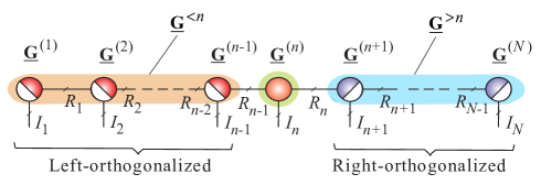
(b)

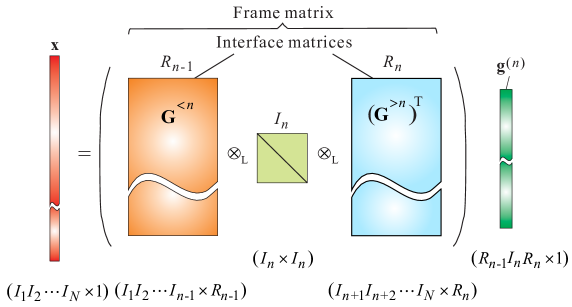
Figure 3.1: Extraction of a single core from a TT network. (a) Representation of a tensor train by the left- and right-orthogonalized sub-trains, with respect to the $n$th core. (b) Graphical illustration of a linear frame equation expressed via a frame matrix or, equivalently, via interface matrices (see Eqs. (3.4) and (3.5)).

Through basic multilinear algebra, we can construct a set of linear equations, referred to as the frame equation, given by

$${\bf x}={\bf G}_{\neq\,n}\;{\bf g}^{(n)},\qquad n=1,2,\ldots,N,$$ (3.4)

where ${\bf x}=\mbox{vec}(\underline{{\bf X}})\in\mathbb{R}^{I_{1}I_{2}\cdots I_{N}}$, $\;\;{\bf g}^{(n)}=\mbox{vec}(\underline{{\bf G}}^{(n)})\in\mathbb{R}^{R_{n-1}I_{n}R_{n}}$, while a tall-and-skinny matrix, ${\bf G}_{\neq n}$, called the frame matrix, is formulated as

$${\bf G}_{\neq\,n}={\bf G}^{<n}\;\otimes_{L}\;{\bf I}_{I_{n}}\;\otimes_{L}\;({\bf G}^{>n})^{\text{T}}\in\mathbb{R}^{I_{1}I_{2}\cdots I_{N}\times R_{n-1}I_{n}R_{n}}.\\$$ (3.5)

Remark. From Eqs. (3.4) and (3.5), observe that the frame and interface matrices indicate an important property of the TT format – its linearity with respect to each core $\underline{{\bf G}}^{(n)}$, when expressed in the vectorized form (see Figure 3.1(b)).

Another important advantage of this approach is that by splitting the TT cores, we can express the data tensor in the following matrix form (see Figure 3.2 for $n=p$)

$$\widetilde{\bf X}_{k_{n}}={\bf G}^{<n}\;{\bf G}_{k_{n}}^{(n)}\;{\bf G}^{>n}\in\mathbb{R}^{I_{1}\cdots I_{n-1}\times I_{n+1}\cdots I_{N}},$$ (3.6)

where $\widetilde{\bf X}_{k_{n}}$ are lateral slices of a 3rd-order reshaped raw tensor, $\tilde{\underline{{\bf X}}}\in\mathbb{R}^{I_{1}\cdots I_{n-1}\;\times\;I_{n}\;\times\;I_{n+1}\cdots I_{N}}$, and $n=1,2,\ldots,N,\;\;i_{n}=1,2,\ldots,I_{n}$, (obtained by reshaping an $N$th-order data tensor $\underline{{\bf X}}\in\mathbb{R}^{I_{1}\;\times I_{2}\;\times\;\cdots\;\times I_{N}}$). Assuming that the columns of ${\bf G}^{<n}$ and the rows of ${\bf G}^{>n}$ are orthonormalized, the lateral slices of a core tensor $\underline{{\bf G}}^{(n)}$ can be expressed as

$${\bf G}^{(n)}_{i_{n}}=({\bf G}^{<n})^{\text{T}}\;\widetilde{\bf X}_{i_{n}}\;({\bf G}^{>n})^{\text{T}}\in\mathbb{R}^{R_{n-1}\;\times\;R_{n}}.$$ (3.7)

(a)

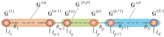
(b)

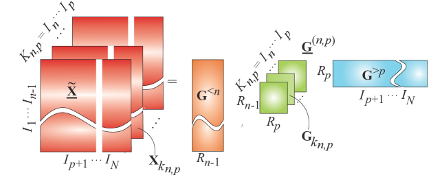
Figure 3.2: Procedure for the extraction of an arbitrary group of cores from a TT network. (a) Splitting a TT network into three TT sub-networks. (b) Reshaping an $N$th-order data tensor to a 3rd-order tensor and its decomposition using the Tucker-2/PVD model. This procedure can be implemented for any $n=1,2,\ldots,N-1$ and $p>n$.

3.1.2 Extraction of Two Neighboring Cores for Modified ALS (MALS)

The Modified ALS algorithm, also called the two-site Density Matrix Renormalization Group (DMRG2) algorithm requires the extraction of two neighboring cores [Holtz et al., 2012a].

Similarly to the previous section, the extraction of a block of two neighboring TT cores is based on the following linear equation

$${\bf x}={\bf G}_{\neq\,n,n+1}\;{\bf g}^{(n,n+1)},\qquad n=1,2,\ldots,N-1,\\$$ (3.8)

where the frame (tall-and-skinny) matrix is formulated as

$${\bf G}_{\neq\,n,n+1} = {\bf G}^{<n}\;\otimes_{L}\;{\bf I}_{I_{n}}\;\otimes_{L}\;{\bf I}_{I_{n+1}}\;\otimes_{L}\;({\bf G}^{>n+1})^{\text{T}}$$ (3.9)

$$\in \mathbb{R}^{I_{1}I_{2}\cdots I_{N}\times R_{n-1}I_{n}I_{n+1}R_{n+1}}$$

and ${\bf g}^{(n,n+1)}=\mbox{vec}({\bf G}^{(n)\;\text{T}}_{L}{\bf G}^{(n+1)}_{R})=\mbox{vec}(\underline{{\bf G}}^{(n,n+1)})\in\mathbb{R}^{R_{n-1}I_{n}I_{n+1}R_{n+1}}$, for $n=1,2,\ldots,N-1$ (see Figure 3.3).

(a)

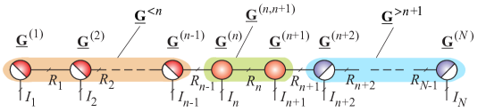
(b)

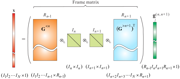
Figure 3.3: Extraction of two neighboring cores. (a) Graphical representation of a tensor train and the left- and right-orthogonalized sub-trains. (b) Graphical illustration of the linear frame equation (see Eqs. (3.8) and (3.9)).

Table 3.1: Basic recursive formulas for the TT/MPS decomposition of an $N$th-order tensor $\underline{{\bf X}}=\mathopen{\hbox{\set@color${\langle}$}\kern-1.94444pt\leavevmode\hbox{\set@color${\langle}$}}\underline{{\bf G}}^{(1)},\underline{{\bf G}}^{(2)},\ldots,\underline{{\bf G}}^{(N)}\mathclose{\hbox{\set@color${\rangle}$}\kern-1.94444pt\leavevmode\hbox{\set@color${\rangle}$}}\in\mathbb{R}^{I_{1}\times\cdots\times I_{N}}$, where $\;\underline{{\bf G}}^{(n)}\in\mathbb{R}^{R_{n-1}\times I_{n}\times R_{n}}$, $\;{\bf G}^{(n)}_{(1)}\in\mathbb{R}^{R_{n-1}\times I_{n}R_{n}}$, $\;{\bf G}^{(n)}_{(2)}\in\mathbb{R}^{I_{n}\times R_{n-1}R_{n}}$, $\;{\bf G}^{(n)}_{<2>}=[{\bf G}^{(n)}_{(3)}]^{\text{T}}\in\mathbb{R}^{R_{n-1}I_{n}\times R_{n}}$, and $\;\;\underline{{\bf X}}=\underline{{\bf G}}^{\leq N}=\underline{{\bf G}}^{\geq 1}$, $\;\;\underline{{\bf G}}^{\leq 0}=\underline{{\bf G}}^{\geq N+1}=1$.

TT (global) TT (recursive) Multilinear products $\displaystyle\underline{{\bf X}}=\underline{{\bf G}}^{(1)}\times^{1}\underline{{\bf G}}^{(2)}\times^{1}\cdots\times^{1}\underline{{\bf G}}^{(N)}$ $\displaystyle\underline{{\bf G}}^{\leq n}=\underline{{\bf G}}^{\leq n-1}\times^{1}\underline{{\bf G}}^{(n)}$ $\displaystyle\underline{{\bf G}}^{\geq n}=\underline{{\bf G}}^{(n)}\times^{1}\underline{{\bf G}}^{\geq n+1}$ Vectorizations $\displaystyle\text{vec}(\underline{{\bf X}})=\prod_{n=N}^{1}\left({\bf G}^{(n)\;\text{T}}_{(1)}\otimes{\bf I}_{I_{1}I_{2}\cdots I_{n-1}}\right)$ $\displaystyle\text{vec}(\underline{{\bf G}}^{\leq n})=$ $=\displaystyle\left({\bf G}^{(n)\;\text{T}}_{(1)}\otimes{\bf I}_{I_{1}I_{2}\cdots I_{n-1}}\right)\text{vec}\left(\underline{{\bf G}}^{\leq n-1}\right)$ $\displaystyle\text{vec}(\underline{{\bf X}})=\prod_{n=1}^{N}\left({\bf I}_{I_{n+1}\cdots I_{N}}\otimes{\bf G}^{(n)}_{<2>}\right)$ $\displaystyle\text{vec}\left(\underline{{\bf G}}^{\geq n}\right)=$ $\displaystyle=\left({\bf I}_{I_{n+1}I_{n+2}\cdots I_{N}}\otimes{\bf G}^{(n)}_{<2>}\right)\text{vec}\left(\underline{{\bf G}}^{\geq n+1}\right)$ $\displaystyle\text{vec}(\underline{{\bf X}})=\left(({\bf G}^{>n}_{(1)})^{\text{T}}\otimes{\bf I}_{I_{n}}\otimes({\bf G}^{<n}_{(n)})^{\text{T}}\right)\text{vec}\left(\underline{{\bf G}}^{(n)}\right)$ Matricizations $\displaystyle{\bf X}_{(n)}={\bf G}^{(n)}_{(2)}\left({\bf G}^{>n}_{(1)}\otimes{\bf G}^{<n}_{(n)}\right)$ $\displaystyle{\bf G}^{<n}_{(n)}={\bf G}^{(n-1)}_{(3)}\left({\bf I}_{I_{n-1}}\otimes{\bf G}^{<n-1}_{(n-1)}\right)$ $\displaystyle{\bf X}_{<n>}={\bf G}^{\leq n}_{<n>}{\bf G}^{>n}_{(1)}=\left({\bf G}^{<n+1}_{(n+1)}\right)^{\text{T}}{\bf G}^{>n}_{(1)}$ $\displaystyle{\bf G}^{\geq n}_{(1)}={\bf G}^{(n)}_{(1)}\left({\bf G}^{\geq n+1}_{(1)}\otimes{\bf I}_{I_{n}}\right)$ $\displaystyle{\bf X}_{<n>}=\left({\bf I}_{I_{n}}\otimes{\bf G}^{\leq n-1}_{<n-1>}\right){\bf G}^{(n)}_{<2>}{\bf G}^{\geq n+1}_{(1)}$ $\displaystyle{\bf X}_{<n-1>}={\bf G}^{\leq n-1}_{<n-1>}{\bf G}^{(n)}_{(1)}\left({\bf G}^{\geq n+1}_{(1)}\otimes{\bf I}_{I_{n}}\right)$ Slice products $\displaystyle x_{i_{1},i_{2},\ldots,i_{N}}={\bf G}^{(1)}_{i_{1}}{\bf G}^{(2)}_{i_{2}}\cdots{\bf G}^{(N)}_{i_{N}}$ $\displaystyle{\bf G}^{\leq n}_{i_{1},\ldots,i_{n}}={\bf G}^{\leq n-1}_{i_{1},\ldots,i_{n-1}}{\bf G}^{(n)}_{i_{n}}$ $\displaystyle{\bf G}^{\geq n}_{i_{n},\ldots,i_{N}}={\bf G}^{(n)}_{i_{n}}{\bf G}^{\geq n+1}_{i_{n+1},\ldots,i_{N}}$

Simple matrix manipulations now yield the following useful recursive formulas (see also Table 3.1)

$${\bf X}_{(n)} = {\bf G}^{(n)}_{(2)}\;({\bf G}^{<n}_{(n)}\otimes_{L}{\bf G}_{(1)}^{>n}),$$ (3.10)

$${\bf G}_{\neq\;n} = {\bf G}_{\neq\;n,n+1}\;({\bf I}_{R_{n-1}I_{n}}\otimes_{L}({\bf G}^{(n+1)}_{(1)})^{\text{T}}),$$ (3.11)

$${\bf G}_{\neq\;n+1} = {\bf G}_{\neq\;n,n+1}\;(({\bf G}^{(n)}_{(3)})^{\text{T}}\;\otimes_{L}\;{\bf I}_{I_{n+1}R_{n+1}}).$$ (3.12)

If the cores are normalized in a such way that all cores to the left of the currently considered (optimized) TT core $\underline{{\bf G}}^{(n)}$ are left-orthogonal

$${\bf G}_{(3)}^{(k)}\;{\bf G}_{(3)}^{(k)\;\text{T}}={\bf G}_{<2>}^{(k)\;\text{T}}\;{\bf G}_{<2>}^{(k)}={\bf I}_{R_{k}},\quad k<n,$$ (3.13)

and all the cores to the right of $\underline{{\bf G}}^{(n)}$ are right-orthogonal

$${\bf G}_{(1)}^{(p)}\;{\bf G}_{(1)}^{(p)\;\text{T}}={\bf G}_{<1>}^{(p)}\;{\bf G}_{<1>}^{(p)\;\text{T}}={\bf I}_{R_{p-1}},\quad p>n,$$ (3.14)

then the frame matrices have orthogonal columns [Pižorn and Verstraete, 2012, Dolgov et al., 2014, Kressner et al., 2014a], that is

$${\bf G}_{\neq\,n}^{\text{T}}\;{\bf G}_{\neq\;n} = {\bf I}_{R_{n-1}\,I_{n}\,R_{n}},$$ (3.15)

$${\bf G}_{\neq\,n,n+1}^{\text{T}}\;{\bf G}_{\neq\,n,n+1} = {\bf I}_{R_{n-1}\,I_{n}\,I_{n+1}\,R_{n+1}}.$$ (3.16)

Figure 3.2 illustrates that the operation of splitting the TT cores into three sub-networks can be expressed in the following matrix form (for $p=n+1$)

$$\widetilde{\bf X}_{k_{n,n+1}}={\bf G}^{<n}\;{\bf G}_{k_{n,n+1}}^{(n,n+1)}\;{\bf G}^{>n+2}\in\mathbb{R}^{I_{1}\cdots I_{n-1}\;\times\;I_{n+2}\cdots I_{N}},$$ (3.17)

for $n=1,2,\ldots,N-1,\;\;k_{n,n+1}=1,2,\ldots,I_{n}I_{n+1}$, where $\widetilde{\bf X}_{k_{n,n+1}}$ are the frontal slices of a 3rd-order reshaped data tensor $\tilde{\underline{{\bf X}}}\in\mathbb{R}^{I_{1}\cdots I_{n-1}\;\times\;I_{n}I_{n+1}\;\times\;I_{n+2}\cdots I_{N}}$.

Assuming that the columns of ${\bf G}^{<n}$ and rows of ${\bf G}^{>n+2}$ are orthonormalized, the frontal slices of a super-core tensor, $\underline{{\bf G}}^{(n,n+1)}\in\mathbb{R}^{R_{n-1}\times I_{n}I_{n+1}\times R_{n+1}}$, can be expressed in the following simple form

$${\bf G}^{(n,n+1)}_{k_{n,n+1}}=({\bf G}^{<n})^{\text{T}}\;\widetilde{\bf X}_{k_{n,n+1}}\;({\bf G}^{>n+2})^{\text{T}}\in\mathbb{R}^{R_{n-1}\times R_{n+1}}.$$ (3.18)

3.2 Alternating Least Squares (ALS) and Modified ALS (MALS)

Consider the minimization of a scalar cost (energy) function, $J(\underline{{\bf X}})$, of an $N$th-order tensor variable expressed in the TT format as $\underline{{\bf X}}\cong\mathopen{\hbox{\set@color${\langle}$}\kern-1.94444pt\leavevmode\hbox{\set@color${\langle}$}}\underline{{\bf X}}^{(1)},\underline{{\bf X}}^{(2)},\ldots,\underline{{\bf X}}^{(N)}\mathclose{\hbox{\set@color${\rangle}$}\kern-1.94444pt\leavevmode\hbox{\set@color${\rangle}$}}$. The solution is sought in the form of a tensor train; however, the simultaneous minimization over all cores $\underline{{\bf X}}^{(n)}$ is usually too complex and nonlinear. For feasibility, the procedure is replaced by a sequence of optimizations carried out over one core at a time, that is $\underline{{\bf X}}^{(n)}=\operatornamewithlimits{\arg\min}J(\underline{{\bf X}}^{(1)},\ldots,\underline{{\bf X}}^{(n)},\ldots,\underline{{\bf X}}^{(N)})$.

The idea behind the Alternating Least Squares (ALS) optimization (also known as the Alternating Linear Scheme or one-site DMRG (DMRG1)) is that in each local optimization (called the micro-iteration step), only one core tensor, $\underline{{\bf X}}^{(n)}$, is updated, while all other cores are kept fixed. Starting from some initial guess for all cores, the method first updates, say, core $\underline{{\bf X}}^{(1)}$, while cores $\underline{{\bf X}}^{(2)},\ldots\underline{{\bf X}}^{(N)}$, are fixed, then it updates $\underline{{\bf X}}^{(2)}$ with $\underline{{\bf X}}^{(1)},\underline{{\bf X}}^{(3)},\ldots,\underline{{\bf X}}^{(n)}$ fixed and so on, until $\underline{{\bf X}}^{(N)}$ is optimized. After completing this forward half-sweep, the algorithm proceeds backwards along the sequence of cores $N,N-1,\ldots,1$, within the so-called backward half-sweep. The sequence of forward and backward iterations complete one full sweep, which corresponds to one (global-) iteration. These iterations are repeated until some stopping criterion is satisfied, as illustrated in Algorithm 7 and Figure 3.4.

0:  Cost (energy) function $J(\underline{{\bf X}})$ and an initial guess for an $N$th-order tensor in the TT format $\underline{{\bf X}}=\mathopen{\hbox{\set@color${\langle}$}\kern-1.94444pt\leavevmode\hbox{\set@color${\langle}$}}\underline{{\bf X}}^{(1)},\underline{{\bf X}}^{(2)},\ldots,\underline{{\bf X}}^{(N)}\mathclose{\hbox{\set@color${\rangle}$}\kern-1.94444pt\leavevmode\hbox{\set@color${\rangle}$}}$ 0:  A tensor $\underline{\mathbf{X}}$ in the TT format minimizes the cost function $J(\underline{\mathbf{X}})$ 1:  while Stopping condition not fulfilled do 2:     for $n=1$ to $N$ do 3:         Find: $\hat{\underline{{\bf X}}}^{(n)}=\displaystyle\mathop{\rm arg\,min}_{\underline{{\bf X}}^{(n)}_{*}}J(\hat{\underline{{\bf X}}}^{(1)},\ldots,\hat{\underline{{\bf X}}}^{(n-1)},\underline{{\bf X}}_{*}^{(n)},\underline{{\bf X}}^{(n+1)},\ldots,\underline{{\bf X}}^{(N)})$ 4:     end for 5:  end while

Algorithm 7 Alternating Least Squares (ALS)

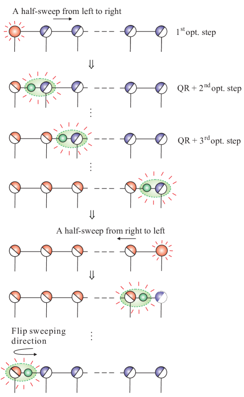
Figure 3.4: The ALS algorithm for TT decomposition corresponding to the DMRG1. The idea is to optimize only one core tensor at a time (by the minimization of a suitable cost function), while keeping the other cores fixed. Optimization of each core tensor is followed by an orthogonalization step via the QR/LQ decompositions. Factor matrices ${\bf R}$ are absorbed (incorporated) into the subsequent core. The small green circle denotes a triangular matrix ${\bf R}$ or ${\bf L}$ which is merged with a neighbouring TT core (as indicted by the green shaded ellipsoid).

As in any iterative optimization based on gradient descent, the cost function can only decrease, however, there is no guarantee that a global minimum would be reached. Also, since the TT rank for the desired solution is unknown, the standard ALS relies on an initial guess for the TT rank; for some initial conditions the iteration process can therefore be very slow. To alleviate these problems, the modified ALS (MALS/DMRG2) scheme aims to merge two neighboring TT cores (blocks), optimize the resulting “super-node” also called “super-core” or “super-block”, and split again the result into separate factors by low-rank matrix factorizations, usually using truncated SVD .

Some remarks:

• If the global cost (loss) function $J(\underline{{\bf X}})$ is quadratic, so too are the local cost functions $J_{n}(\underline{{\bf X}}^{(n)})$, and the problem reduces to solving a small-scale optimization at each micro-iteration. In addition, local problems in the micro-iterations are usually better conditioned, due to the orthogonalization of TT cores.

• In most optimization problems considered in this monograph the TT decomposition is assumed to be in an orthogonalized form, where all cores are left– or right–orthogonal with respect to the core $\underline{{\bf X}}^{(n)}$, which is being optimized (see also Figure 3.4 and Figure 3.5) [Holtz et al., 2012a, Dolgov and Khoromskij, 2013].

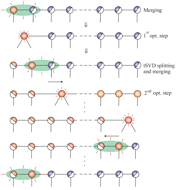
Figure 3.5: The Modified ALS (MALS) algorithm corresponding to the DMRG2. In every optimization step, two neighboring cores are merged and the optimization is performed over the so obtained “super-core”. In the next step, truncated SVD or other low-rank matrix factorizations (LRMF) are applied in order to split the optimized super-core into two cores. Note that each optimization sub-problem is computationally more expensive than the standard ALS. During the iteration process, convergence speed may increase considerably as compared to the standard ALS algorithm, and TT ranks can be adaptively estimated.

3.3 Tensor Completion for Large-Scale Structured Data

The objective of tensor completion is to reconstruct a high-dimensional structured multiway array for which a large proportion of entries is missing or noisy [Grasedyck et al., 2015, Steinlechner, 2016a, b, Zhao et al., 2015, 2016, Yokota et al., 2016].

With the assumption that a good low-rank TN approximation for an incomplete data tensor $\underline{{\bf Y}}\in\mathbb{R}^{I_{1}\times I_{2}\times\cdots\times I_{N}}$ does exist, the tensor completion problem can be formulated as the following optimization problem

$$\min_{\underline{{\bf X}}}\;J(\underline{{\bf X}})=\|P_{\Omega}(\underline{{\bf Y}})-P_{\Omega}(\underline{{\bf X}})\|_{F}^{2}$$ (3.19)

subject to $\underline{{\bf X}}\in{\cal{M}}_{R}:=\{\underline{{\bf X}}\in\mathbb{R}^{I_{1}\times I_{2}\times\cdots\times I_{N}}\;|\;\mbox{rank}_{TT}(\underline{{\bf X}})={\bf r}_{TT}\}$, where $\underline{{\bf X}}$ is the reconstruction tensor in TT format and ${\bf r}_{TT}=\{R_{1},R_{2},\ldots,R_{N-1}\}$. The symbol $P_{\Omega}$ denotes the projection onto the sampling set $\Omega$ which corresponds to the indices of the known entries of $\underline{{\bf Y}}$, i.e., $P_{\Omega}(\underline{{\bf Y}}(i_{1},i_{2},\ldots,i_{N}))=\underline{{\bf Y}}(i_{1},i_{2},\ldots,i_{N})$ if $(i_{1},i_{2},\ldots,i_{N})\in\Omega$, otherwise zero.

For a large-scale high-order reconstruction tensor represented in the TT format, that is, $\underline{{\bf X}}=\mathopen{\hbox{\set@color${\langle}$}\kern-1.94444pt\leavevmode\hbox{\set@color${\langle}$}}\underline{{\bf X}}^{(1)},\underline{{\bf X}}^{2)},\ldots,\underline{{\bf X}}^{(N)}\mathclose{\hbox{\set@color${\rangle}$}\kern-1.94444pt\leavevmode\hbox{\set@color${\rangle}$}}$, the above optimization problem can be converted by the ALS approach to a set of smaller optimization problems. These can be represented in a scalar form through slices of core tensors, as follows

$$\widehat{\underline{{\bf X}}}^{(n)}=\mbox{arg}\min_{\underline{{\bf X}}^{(n)}}\,\sum_{{\bf i}\in\Omega}\biggl{(}\underline{{\bf Y}}(i_{1},\ldots,i_{N})-{\bf X}^{(1)}_{i_{1}}\cdots{\bf X}^{(n)}_{i_{n}}{\bf X}^{(n+1)}_{i_{n}}\cdots{\bf X}^{(N)}_{i_{N}}\biggr{)}^{\!2}.$$

For convergence, it is necessary to iterate through all cores, $\underline{{\bf X}}^{(n)}$, $n=1,2,\ldots,N$, and over several sweeps.

For efficiency, all the cores are orthogonalized after each sweep, and the cost function is minimized in its vectorized form by sequentially minimizing each individual slice, ${\bf X}^{(n)}_{i_{n}}$, of the cores, $\underline{{\bf X}}^{(n)}\in\mathbb{R}^{R_{n-1}\times I_{n}\times R_{n}}$ (see also formulas (3.6) and (3.7)), that is

$$\widehat{{\bf X}}^{(n)}_{i_{n}} = \mbox{arg}\min_{{\bf X}^{(n)}_{i_{n}}}\,\|\mbox{vec}(\widetilde{\underline{{\bf Y}}}_{i_{n}})-\mbox{vec}({\bf X}^{<n}\;{\bf X}^{(n)}_{i_{n}}\;{\bf X}^{>n})\|_{\Omega}^{2}$$

$$= \mbox{arg}\min_{{\bf X}^{(n)}_{i_{n}}}\,\|\mbox{vec}(\widetilde{\underline{{\bf Y}}}_{i_{n}}-[{\bf X}^{<n}\;\otimes_{L}\;({\bf X}^{>n})^{\text{T}}]\mbox{vec}({\bf X}^{(n)}_{i_{n}})\|_{\Omega}^{2},$$

for all $i_{n}=1,2,\ldots,I_{n}$ and $n=1,2,\ldots,N$, where $\|{\bf v}\|_{\Omega}^{2}=\sum_{i\in\Omega}v_{i}^{2}$.

The above optimization problem for $\mbox{vec}({\bf X}^{(n)}_{i_{n}})$ can be considered as a standard linear least squares (LS) problem, which can be efficiently solved even for huge-scale datasets.

In general, TT ranks are not known beforehand and must be estimated during the optimization procedure. These can be estimated by, for example, starting with a maximum rank $R_{\max}$ and reducing gradually ranks by TT rounding. Alternatively, starting from a minimum rank, $R_{\min}$, the ranks could be gradually increased. The rank increasing procedure can start with ${\bf r}_{TT}=\{1,1,\ldots,1\}$, and the so obtained result is used for another run (sweep), but with ${\bf r}_{TT}=\{1,2,\ldots,1\}$. In other words, the rank $R_{2}$ between the second and third core is increased, and so on until either the prescribed residual tolerance $\varepsilon$ or $R_{\max}$ is reached. As the rank value is a key factor which determines the complexity of the ALS, the second approach is often more efficient and is computationally comparable with rank-adaptive approaches [Grasedyck et al., 2015, Steinlechner, 2016a, b].

3.4 Computing a Few Extremal Eigenvalues and Eigenvectors

3.4.1 TT Network for Computing the Single Smallest Eigenvalue and the Corresponding Eigenvector

Machine learning applications often require the computation of extreme (minimum or maximum) eigenvalues and the corresponding eigenvectors of large-scale structured symmetric matrices. This problem can be formulated as the standard symmetric eigenvalue decomposition (EVD), in the form

$${\bf A}\,{\bf x}_{k}=\lambda_{k}{\bf x}_{k},\qquad k=1,2,\ldots,K,$$ (3.21)

where ${\bf x}_{k}\in\mathbb{R}^{I}$ are the orthonormal eigenvectors and $\lambda_{k}$ the corresponding eigenvalues of a symmetric matrix ${\bf A}\in\mathbb{R}^{I\times I}$.

Iterative algorithms for extreme eigenvalue problems often exploit the Rayleigh Quotient (RQ) of a symmetric matrix as the following cost function

$$J({\bf x})=R({\bf x},{\bf A})=\frac{{\bf x}^{\text{T}}{\bf A}{\bf x}}{{\bf x}^{\text{T}}{\bf x}}=\frac{\langle{\bf A}{\bf x},{\bf x}\rangle}{\langle{\bf x},{\bf x}\rangle},\qquad{\bf x}\neq 0.$$ (3.22)

Based on the Rayleigh Quotient (RQ), the largest, $\lambda_{max}$, and smallest, $\lambda_{min}$, eigenvalue of the matrix ${\bf A}$ can be computed as

$$\lambda_{max}=\max_{{\bf x}}R({\bf x},{\bf A}),\quad\lambda_{min}=\min_{{\bf x}}R({\bf x},{\bf A}),$$ (3.23)

while the critical points and critical values of $R({\bf x},{\bf A})$ are the corresponding eigenvectors and eigenvalues of ${\bf A}$.

The traditional methods for solving eigenvalue problems for a symmetric matrix, ${\bf A}\in\mathbb{R}^{I\times I}$, are prohibitive for very large values of $I$, say $I=10^{15}$ or higher. This computational bottleneck can be very efficiently dealt with through low-rank tensor approximations, and the last 10 years have witnessed the development of such techniques for several classes of optimization problems, including EVD/PCA and SVD [Dolgov et al., 2014, Kressner et al., 2014a, Lee and Cichocki, 2015]. The principle is to represent the cost function in a tensor format; under certain conditions, such as that tensors can be often quite well approximated in a low-rank TT format, thus allowing for low-dimensional parametrization.

In other words, if a structured symmetric matrix ${\bf A}$ and its eigenvector ${\bf x}$ admit low-rank TT approximations, a large-scale eigenvalue problem can be converted into a set of smaller optimization problems by representing the eigenvector, ${\bf x}\in\mathbb{R}^{I}$, and the matrix, ${\bf A}\in\mathbb{R}^{I\times I}$, in TT (MPS/MPO) formats, i.e., a TT/MPS for an $N$th-order tensor $\underline{{\bf X}}\cong\mathopen{\hbox{\set@color${\langle}$}\kern-1.94444pt\leavevmode\hbox{\set@color${\langle}$}}\underline{{\bf X}}^{(1)},\ldots,\underline{{\bf X}}^{(N)}\mathclose{\hbox{\set@color${\rangle}$}\kern-1.94444pt\leavevmode\hbox{\set@color${\rangle}$}}\in\mathbb{R}^{I_{1}\times\cdots\times I_{N}}$ and a matrix TT/MPO for a $2N$th-order tensor $\underline{{\bf A}}\cong\mathopen{\hbox{\set@color${\langle}$}\kern-1.94444pt\leavevmode\hbox{\set@color${\langle}$}}\underline{{\bf A}}^{(1)},\ldots,\underline{{\bf A}}^{(N)}\mathclose{\hbox{\set@color${\rangle}$}\kern-1.94444pt\leavevmode\hbox{\set@color${\rangle}$}}\in\mathbb{R}^{I_{1}\times I_{1}\times\cdots\times I_{N}\times I_{N}}$, where $I=I_{1}I_{2}\cdots I_{N}$.

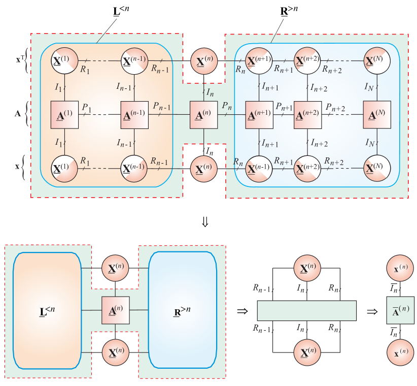
Figure 3.6: A conceptual TT network for the computation of a single extreme eigenvalue, $\lambda$, and the corresponding eigenvector, ${\bf x}\in\mathbb{R}^{I}$, for a symmetric matrix ${\bf A}\in\mathbb{R}^{I\times I}$. The frame matrix maps the TT core into a large vector. The tensor network corresponds to the cost function (quadratic form), ${\bf x}^{\text{T}}{\bf A}{\bf x}$, where the matrix ${\bf A}$ and vectors ${\bf x}\in\mathbb{R}^{I}$ are given in the tensor train format with distributed indices $I=I_{1}I_{2}\cdots I_{N}$. The cores in the shaded areas form the matrix $\overline{\bf A}^{(n)}$ (the effective Hamiltonian), which can be computed by a sequentially optimized contraction of the TT cores.

Figure 3.6 illustrates this conversion into a set of much smaller sub-problems by employing tensor contractions and the frame equations (see section 3.1)

$${\bf x}={\bf X}_{\neq n}\,{\bf x}^{(n)},\qquad n=1,2,\ldots,N,$$ (3.24)

with the frame matrices

$${\bf X}_{\neq n}={\bf X}^{<n}\otimes_{L}{\bf I}_{I_{n}}\otimes_{L}({\bf X}^{>n})^{\text{T}}\in\mathbb{R}^{I_{1}I_{2}\cdots I_{N}\times R_{n-1}I_{n}R_{n}}.$$ (3.25)

Since the cores $\underline{{\bf X}}^{(m)}$ for $m\neq n$ are constrained to be left- or right-orthogonal, the RQ can be minimized (or maximized), as follows

$$\min_{{\bf x}}\,J({\bf x}) = \min_{{\bf x}^{(n)}}\,J({\bf X}_{\neq n}{\bf x}^{(n)})$$

$$= \min_{{\bf x}^{(n)}}\frac{{\bf x}^{(n)\;\text{T}}\;\overline{\bf A}^{(n)}\;{\bf x}^{(n)}}{\langle{\bf x}^{(n)},{\bf x}^{(n)}\rangle},\quad n=1,2,\ldots,N,\quad$$

where ${\bf x}^{(n)}=\mbox{vec}(\underline{{\bf X}}^{(n)})\in\mathbb{R}^{R_{n-1}I_{n}R_{n}}$ and the matrix $\overline{\bf A}^{(n)}$ (called the effective Hamiltonian) can be expressed as

$$\overline{\bf A}^{(n)}=({\bf X}_{\neq n})^{\text{T}}{\bf A}{\bf X}_{\neq n}\in\mathbb{R}^{R_{n-1}I_{n}R_{n}\times R_{n-1}I_{n}R_{n}}$$ (3.27)

for $n=1,2,\ldots,N$, under the condition $({\bf X}_{\neq n})^{\text{T}}{\bf X}_{\neq n}={\bf I}$.

For relatively small TT ranks, the matrices $\overline{\bf A}^{(n)}$ are usually much smaller than the original matrix ${\bf A}$, so that a large-scale EVD problem can be converted into a set of much smaller EVD sub-problems, which requires solving the set of equations

$$\overline{\bf A}^{(n)}\,{\bf x}^{(n)}=\lambda{\bf x}^{(n)},\quad n=1,2,\ldots,N.$$ (3.28)

In practice, the matrices $\overline{\bf A}^{(n)}$ are never computed directly by (3.27). Instead, we compute matrix-by-vector multiplication, ${\bf A}^{(n)}\,{\bf x}^{(n)}$, iteratively via optimized contraction of TT cores within a tensor network. The concept of optimized contraction is illustrated in Figure 3.7.

(a)

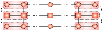
(b)

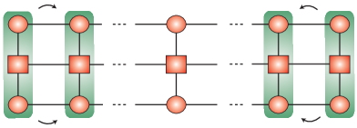
(c)

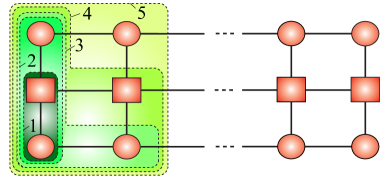
Figure 3.7: Sequential contraction of the TT network. (a) Sub-optimal (inefficient) and (b) Optimal (efficient) contraction of the TT (MPS/MPO) network. (c) Details of optimal sequential contraction (the numbers $1,2,3,\ldots$ indicate the order of tensor contractions).

It should be noted that the contraction of the matrix ${\bf A}$ in TT/MPO format, with corresponding TT cores of the vectors ${\bf x}$ and ${\bf x}^{\text{T}}$ in TT/MPS format, leads to the left- and right contraction tensors $\underline{{\bf L}}^{<n}$ and $\underline{{\bf R}}^{>n}$, as illustrated in Figure 3.6. In other words, efficient solution of the matrix equation (3.28) requires computation of the blocks $\underline{{\bf L}}^{<n}$ and $\underline{{\bf R}}^{>n}$; these can be built iteratively so as to best reuse available information, which involves an optimal arrangement of a tensor network contraction. In a practical implementation, the full network contraction is never carried out globally, but through iterative sweeps from right to left or vice-versa, to build up $\underline{{\bf L}}^{<n}$ and $\underline{{\bf R}}^{>n}$ from the previous steps. The left and right orthogonalization of the cores can also be exploited to simplify the tensor contraction process [Schollwöck, 2011, Dolgov et al., 2014, Kressner et al., 2014a, Lee and Cichocki, 2015, 2016b].

Remark. Before we construct the tensor network shown in the Figure 3.6, we need to construct approximate distributed representation of the matrix ${\bf A}$ in the TT/MPO format. For ways to construct efficient representations of huge-scale matrix in TT/MPO format while simultaneously performing compression see [Hubig et al., 2017, August et al., 2016] and also Part 1 [Cichocki et al., 2016].

3.4.2 TT Network for Computing Several Extremal Eigenvalues and Corresponding Eigenvectors for Symmetric EVD

In a more general case, several (say, $K$) extremal eigenvalues and the corresponding $K$ eigenvectors of a symmetric structured matrix ${\bf A}$ can be computed through the following trace minimization (or maximization) with orthogonality constraints

$$\min_{{\bf X}}\,\mathop{\rm tr}\nolimits({\bf X}^{\text{T}}{\bf A}{\bf X}),\qquad\mbox{s.t.}\;\;{\bf X}^{\text{T}}{\bf X}={\bf I}_{K},$$ (3.29)

where ${\bf X}=[{\bf x}_{1},{\bf x}_{2},\ldots,{\bf x}_{K}]\in\mathbb{R}^{I_{1}I_{2}\cdots I_{N}\;\times\;K}$ is a matrix composed of eigenvectors ${\bf x}_{k}$, and ${\bf A}\in\mathbb{R}^{I\times I}$ is a huge-scale symmetric matrix.

Note that the global minimum of this cost function is equivalent to a sum of $K$ smallest eigenvalues, $\lambda_{1}+\lambda_{2}+\cdots+\lambda_{K}$.

For a very large-scale symmetric matrix ${\bf A}\in\mathbb{R}^{I\times I}$ with say, $I=10^{15}$ or higher, the optimization problem in (3.29) cannot be solved directly. A feasible TT solution would be to first tensorize the matrices ${\bf A}\in\mathbb{R}^{I\times I}$ and ${\bf X}\in\mathbb{R}^{I\times K}$ into the respective tensors $\underline{{\bf A}}\in\mathbb{R}^{I_{1}\times I_{1}\times\cdots\times I_{N}\times I_{N}}$ and $\underline{{\bf X}}\in\mathbb{R}^{I_{1}\times I_{2}\times\cdots\times I_{N}\times K}$, where $I=I_{1}I_{2}\cdots I_{N}$ and the value of every $I_{n}$ is much smaller than $I$; then, a tensor network structure can be exploited to allow a good low-rank TN approximation of the underlying cost function.

Instead of representing each eigenvector ${\bf x}_{k}$ individually in the TT format, we can parameterize them jointly in a block TT format (see Figure 3.8) [Pižorn and Verstraete, 2012, Dolgov et al., 2014]. In general, the block TT format is suitable for approximate representation of tall and skinny structured matrices using almost the same number of data samples as for representation a single vector/matrix. Within the block-$n$ TT, all but one cores are 3rd-order tensors, the remaining core is a 4th-order tensor and has an additional physical index $K$ which represents the number of eigenvectors, as shown in Figure 3.9. The position of this 4th-order core $\underline{{\bf X}}^{(n)}$ which carries the index $K$ is not fixed; during sequential optimization, it is moved backward and forward from position 1 to $N$ [Holtz et al., 2012a, Dolgov et al., 2014]. Observe that this 4th-order core $\underline{{\bf X}}^{(n)}=\left[{\bf X}_{k}^{(n)}\right]^{K}_{k=1}=\left[{\bf X}^{(n,k)}\right]\in\mathbb{R}^{R_{n-1}\times I_{n}\times R_{n}\times K}$ comprises the $K$ different eigenvectors, while all remaining cores retain their original structure. During the optimization process, the neighbouring core tensors need to be appropriately reshaped, as explained in detail in Algorithm 8 and Algorithm 9.

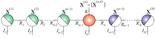
Figure 3.8: Block-$n$ TT with left- and right-orthogonal cores, for an $(N+1)$th-order tensor $\underline{{\bf X}}\in\mathbb{R}^{I_{1}\;\times\;I_{2}\;\times\cdots\times\;I_{N}\;\times\;K}$.

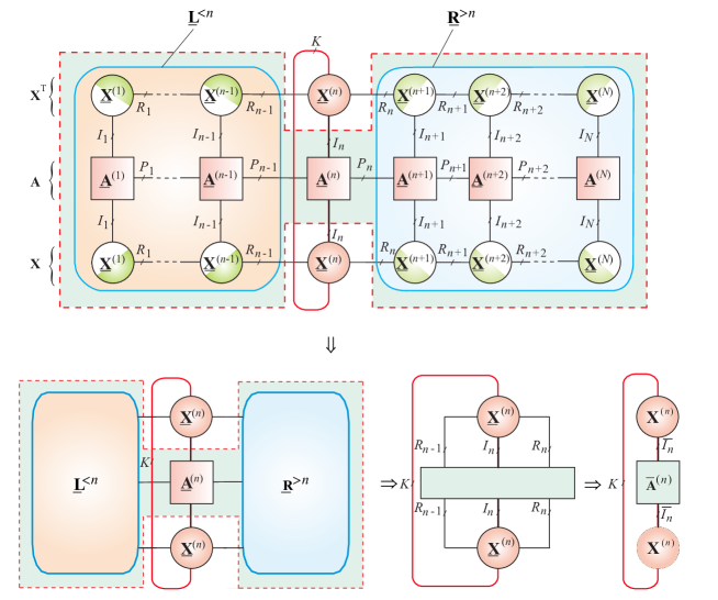
Figure 3.9: Tensor network for the optimization problem in (3.29) and its contraction to reduce the scale of the problem. The network represents a cost function, the minimization of which allows us to compute in the TT format the $K$ eigenvectors corresponding to $K$ extreme eigenvalues. The extreme eigenvalues are computed as $\mbox{\boldmath$\Lambda$}={\bf X}^{(n)\;\text{T}}\;\overline{\bf A}^{(n)}\,{\bf X}^{(n)}$.

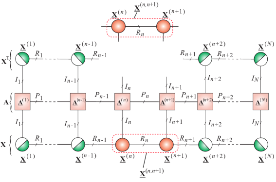
Figure 3.10: Tensor network for the optimization problem in (3.29) and its contraction using the MALS (two-site DMRG2) approach. The network is the same and represents the same cost function as for the ALS but the optimization procedure is slightly different. In this approach, we merge two neighboring cores, optimize them and then split them back to the original cores via the SVD and estimate the optimal rank $R_{n}$ for a prescribed approximation accuracy.

When using the block-$n$ TT model to represent the $K$ mutually orthogonal vectors, the matrix frame equation takes a slightly modified form

$${\bf X}={\bf X}_{\neq n}\;{\bf X}^{(n)}\in\mathbb{R}^{I\times K},\quad n=1,2,\ldots,N,$$ (3.30)

where ${\bf X}^{(n)}={\bf X}^{(n)}_{<3>}={\bf X}^{(n)\;\text{T}}_{(4)}\in\mathbb{R}^{R_{n-1}I_{n}R_{n}\times K}$.

Hence, we can express the trace in (3.29), as follows

$$\mathop{\rm tr}\nolimits({\bf X}^{\text{T}}{\bf A}{\bf X}) = \mathop{\rm tr}\nolimits(({\bf X}_{\neq n}{\bf X}^{(n)})^{\text{T}}{\bf A}{\bf X}_{\neq n}{\bf X}^{(n)})$$ (3.31)

$$= \mathop{\rm tr}\nolimits(({\bf X}^{(n)})^{\text{T}}[{\bf X}_{\neq n}^{\text{T}}{\bf A}{\bf X}_{\neq n}]{\bf X}^{(n)})$$

$$= \mathop{\rm tr}\nolimits({\bf X}^{(n)\,\text{T}}\;\overline{\bf A}^{(n)}\,{\bf X}^{(n)}),$$

where $\overline{\bf A}^{(n)}={\bf X}_{\neq n}^{\text{T}}{\bf A}{\bf X}_{\neq n}$.

0:  $N$th-order tensor, $\underline{{\bf X}}$, in block-$n$ TT format with $n<N$ 0:  The tensor $\underline{{\bf X}}$ in block-$(n+1)$ TT format, with new cores $\underline{{\bf X}}^{(n)}\in\mathbb{R}^{R_{n-1}\;\times I_{n}\;\times\;R_{n}}$ and $\underline{{\bf X}}^{(n+1)}\in\mathbb{R}^{R_{n}\;\times\;I_{n+1}\;\times\;R_{n+1}\;\times K}$ 1:  Reshape the core $\underline{{\bf X}}^{(n)}=\left[\underline{{\bf X}}_{k}^{(n)}\right]^{K}_{k=1}=\left[\underline{{\bf X}}^{(n,k)}\right]\in\mathbb{R}^{R_{n-1}\times I_{n}\times R_{n}\times K}$ into a 3rd-order tensor $\underline{{\bf X}}_{L}^{(n)}\in\mathbb{R}^{R_{n-1}\;I_{n}\;\times\;R_{n}\;\times K}$ 2:  Perform a minimum rank decomposition (using, e.g., QR or SVD) $\underline{{\bf X}}_{L}^{(n)}(:,:,k)={\bf Q}\;{\bf P}_{k}\in\mathbb{R}^{R_{n-1}\,I_{n}\;\times\;R_{n}},\;\;k=1,\ldots,K$ where ${\bf Q}\in\mathbb{R}^{R_{n-1}I_{n}\times R},\qquad{\bf P}_{k}\in\mathbb{R}^{R\;\times\;R_{n}}$ 3:  Update the rank $R_{n}\leftarrow R$ 4:  Update new cores ${\bf X}^{(n)}_{L}\leftarrow{\bf Q},\;\;\;\underline{{\bf X}}_{R}^{(n+1)}(:,:,k)\leftarrow{\bf P}_{k}{\bf X}_{R}^{(n+1)}\in\mathbb{R}^{R_{n}\times I_{n+1}R_{n+1}},\;\;\forall k$ 5:  return  $\underline{{\bf X}}=\mathopen{\hbox{\set@color${\langle}$}\kern-1.94444pt\leavevmode\hbox{\set@color${\langle}$}}\underline{{\bf X}}^{(1)},\ldots,\underline{{\bf X}}^{(n)},\underline{{\bf X}}^{(n+1)},\ldots,\underline{{\bf X}}^{(N)}\mathclose{\hbox{\set@color${\rangle}$}\kern-1.94444pt\leavevmode\hbox{\set@color${\rangle}$}}$

Algorithm 8 Transformation of the block-$n$ TT into the block-$(n+1)$ TT [Dolgov et al., 2014, Kressner et al., 2014a]

0:  $N$th-order tensor, $\underline{{\bf X}}$, in the block-$n$ TT format with $n>1$ 0:  The tensor $\underline{{\bf X}}$ in block-$(n-1)$ TT format, with new cores $\underline{{\bf X}}^{(n-1)}\in\mathbb{R}^{R_{n-2}\;\times\;I_{n-1}\;\times R_{n-1}\;\times\;K}$ and $\underline{{\bf X}}^{(n)}\in\mathbb{R}^{R_{n-1}\;\times\;I_{n}\times\;R_{n}}$ 1:  Reshape the core $\underline{{\bf X}}^{(n)}=\left[\underline{{\bf X}}^{(n,k)}\right]\in\mathbb{R}^{R_{n-1}\;\times\;I_{n}\;\times\;R_{n}\;\times\;K}$ into a 3rd-order tensor for the TT core $\underline{{\bf X}}_{R}^{(n)}\in\mathbb{R}^{R_{n-1}\;\times\;I_{n}R_{n}\times K}$ 2:  Perform a minimum rank decomposition (using, e.g., RQ/LQ) $\underline{{\bf X}}_{R}^{(n)}(:,:,k)={\bf Q}_{k}{\bf P}\in\mathbb{R}^{R_{n-1}\;\times\;I_{n}R_{n}},\;\;k=1,\ldots,K$ where ${\bf Q}_{k}\in\mathbb{R}^{R_{n-1}\;\times\;R},\qquad{\bf P}\in\mathbb{R}^{R\;\times\;I_{n}R_{n}}$ 3:  Update the rank $R_{n-1}\leftarrow R$ 4:  Update new cores ${\bf X}^{(n)}_{R}\leftarrow{\bf P},\;\;\;\underline{{\bf X}}_{L}^{(n-1)}(:,:,k)\leftarrow{\bf X}_{L}^{(n-1)}{\bf Q}_{k}\in\mathbb{R}^{R_{n-2}I_{n-1}\;\times\;R_{n-1}},\;\;\forall k$ 5:  return  $\underline{{\bf X}}=\mathopen{\hbox{\set@color${\langle}$}\kern-1.94444pt\leavevmode\hbox{\set@color${\langle}$}}\underline{{\bf X}}^{(1)},\ldots,\underline{{\bf X}}^{(n-1)},\underline{{\bf X}}^{(n)},\ldots,\underline{{\bf X}}^{(N)}\mathclose{\hbox{\set@color${\rangle}$}\kern-1.94444pt\leavevmode\hbox{\set@color${\rangle}$}}$

Algorithm 9 Transformation of the block-$n$ TT into the block-$(n-1)$ TT [Kressner et al., 2014a]

0:  A symmetric matrix ${\bf A}\in\mathbb{R}^{I\times I}$, and initial guesses for ${\bf X}\in\mathbb{R}^{I_{1}I_{2}\cdots I_{N}\times K}$ in block-1 TT format and with right orthogonal cores $\underline{{\bf X}}^{(2)},\ldots,\underline{{\bf X}}^{(N)}$ 0:  Approximative solution ${\bf X}$ in the TT format 1:  for $n=1$ to $N-1$ do 2:     Perform tensor network contractions (Figure 3.9) and solve a reduced EVD problem (3.31), for the TT core $\underline{{\bf X}}^{(n)}$ 3:     Transform block-$n$ TT to block-$(n+1)$ TT by applying Algorithm 8, such that the updated core ${\bf X}^{(n)}$ is left-orthogonal 4:  end for 5:  for $n=N$ to $2$ do 6:     Perform tensors network contraction and solve a reduced EVD problem (3.31) for the TT core $\underline{{\bf X}}^{(n)}$ 7:     Transform block-$n$ TT to block-$(n-1$) TT by applying Algorithm 9, so that the updated core ${\bf X}^{(n)}$ is right-orthogonal 8:  end for 9:  return  $\underline{{\bf X}}=\mathopen{\hbox{\set@color${\langle}$}\kern-1.94444pt\leavevmode\hbox{\set@color${\langle}$}}\underline{{\bf X}}^{(1)},\underline{{\bf X}}^{(2)},\ldots,\underline{{\bf X}}^{(N)}\mathclose{\hbox{\set@color${\rangle}$}\kern-1.94444pt\leavevmode\hbox{\set@color${\rangle}$}}$

Algorithm 10 One full sweep of the ALS algorithm for symmetric EVD [Dolgov and Savostyanov, 2014]

Assuming that the frame matrices have orthogonal columns, the optimization problem in (3.29) can be converted into a set of linked relatively small-scale optimization problems

$$\min_{{\bf X}^{(n)}}\mathop{\rm tr}\nolimits({\bf X}^{(n)\,\text{T}}\;\overline{\bf A}^{(n)}\,{\bf X}^{(n)}),\quad\mbox{s.t.}\;\;{\bf X}^{(n)\;\text{T}}{\bf X}^{(n)}={\bf I}_{K}$$ (3.32)

for $n=1,2,\ldots,N$, where $\overline{\bf A}^{(n)}$ is computed recursively by tensor network contractions, as illustrated in Figure 3.9. In other words, the EVD problem can be solved iteratively via optimized recursive contraction of the TT network, whereby the active block (i.e., currently optimized core $\underline{{\bf X}}^{(n)}=\left[{\bf X}^{(n,k)}\right]$) is sequentially optimized by sweeping from left to right and back from right to left, and so on, until convergence as illustrated in Algorithm 10 [Dolgov et al., 2014, Kressner et al., 2014a].

During the optimization, the global orthogonality constraint, ${\bf X}^{\text{T}}{\bf X}={\bf I}_{K}$, is equivalent to the set of local orthogonality constraints, $({\bf X}^{(n)})^{\text{T}}{\bf X}^{(n)}={\bf I}_{K},\;\forall n$, so that due to left- and right-orthogonality of the TT cores, we can write

$${\bf X}^{\text{T}}{\bf X} = {\bf X}^{(n)\,T}\;{\bf X}^{\text{T}}_{\neq n}\;{\bf X}_{\neq n}{\bf X}^{(n)}$$

$$= {\bf X}^{(n)\,\text{T}}{\bf X}^{(n)},\;\;\forall n.$$

which allows for a dramatic reduction in computational complexity.

3.4.3 Modified ALS (MALS/DMRG2) for Symmetric EVD

In order to accelerate the convergence speed and improve performance of ALS/DMRG1 methods, the MALS (two-site DMRG2) scheme optimizes, instead of only one, simultaneously two neighbouring TT-cores at each micro-iteration, while the other TT-cores remain fixed (assumed to be known). This reduces a large-scale optimization problem to a set of smaller-scale optimization problems, although the MALS sub-problems are essentially of bigger size than those for the ALS.

After local optimization (micro-iteration) on a merged core tensor, $\underline{{\bf X}}^{(n,n+1)}=\underline{{\bf X}}^{(n)}\times^{1}\underline{{\bf X}}^{(n+1)}$, it is in the next step decomposed (factorized) into two separate TT-cores via a $\delta$-truncated SVD of the unfolded matrix, ${\bf X}^{(n,n+1)}_{<2>}\in\mathbb{R}^{R_{n-1}I_{n}\;\times\;I_{n+1}R_{n+1}}$, as

$$[{\bf U},{\bf S},{\bf V}]=\mbox{tSVD}\left({\bf X}^{(n,n+1)}_{<2>}\right),$$ (3.34)

which allows us to both update the cores, ${\bf X}^{(n)}_{<2>}={\bf U}$ and ${\bf X}^{(n+1)}_{<1>}={\bf S}{\bf V}^{\text{T}}$, and to estimate the TT rank between the cores as $R_{n}=\min(\mbox{size}({\bf U},2),R_{\max})$.

In this way, the TT-ranks can be adaptively determined during the iteration process, while the TT-cores can be left- or right-orthogonalized, as desired. The truncation parameter, $\delta>0$, can be selected heuristically or adaptively (see e.g. [Oseledets and Dolgov, 2012, Lee and Cichocki, 2015]).

The use of truncated SVD allows us to: (1) Estimate the optimal rank, $R_{n}$, and to (2) quantify the error associated with this splitting. In other words, the power of MALS stems from the splitting process which allows for a dynamic control of TT ranks during the iteration process, as well as from the ability to control the level of error of low-rank TN approximations.

3.4.4 Alternating Minimal Energy Method for EVD (EVAMEn)

Recall that the standard ALS method cannot adaptively change the TT ranks during the iteration process, whereas the MALS method achieves this in intermediate steps, through the merging and then splitting of two neighboring TT cores, as shown in the previous section. The cost function $J(\underline{{\bf X}})$ is not convex with respect to all the elements of the core tensors of $\underline{{\bf X}}$ and as consequence the ALS is prone to getting stuck in local minima and suffers from a relatively slow convergence speed. On the other hand, the intermediate steps of the MALS help to alleviate these problems and improve the convergence speed, but there is still not guarantee that the algorithm will converge to a global minimum.

The Alternating Minimal Energy (AMEn) algorithm aims to avoid the problem of convergence to non-global minimum by exploiting the information about the gradient of a cost function or information about the value of a current residual by “enriching” the TT cores with additional information during the iteration process [Dolgov and Savostyanov, 2014]. In that sense, the AMEn can be considered as a subspace correction technique. Such an enrichment was efficiently implemented first by Dolgov and Savostyanov to solve symmetric as well as nonsymmetric linear systems [Dolgov et al., 2016] and was later extended to symmetric EVD in [Kressner et al., 2014a] and [Hubig et al., 2015].

(a)

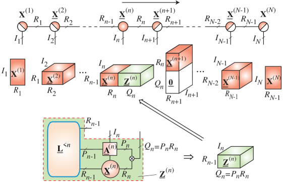
(b)

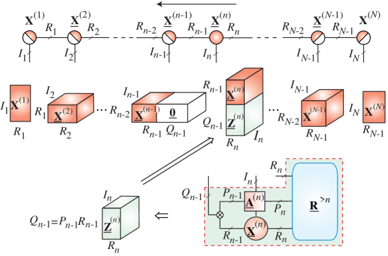
Figure 3.11: Core enrichment step in the AMEn algorithm for the EVD problem, during: (a) Left-to-right half-sweep ($n=1,2,\ldots,N-1$) and (b) Right-to-left half-sweep ($n=N,N-1,\ldots,2$) of the TT network (see also Figure 3.6). At the $n$th micro-iteration, only one core tensor, $\underline{{\bf X}}^{(n)}$, is concatenated (enriched) with a core tensor $\underline{{\bf Z}}^{(n)}$ obtained from the residual, while its neighboring core tensor is formally concatenated with a zero tensor. For simplicity, this is illustrated for $K=1$.

Similar to the ALS method, at each iteration step, the AMEn algorithm updates a single core tensor (see Figure 3.11). Then, it concatenates the updated TT core $\underline{{\bf X}}^{(n)}$ with a core tensor $\underline{{\bf Z}}^{(n)}$ obtained from the residual vector. At each micro-iteration, only one core tensor of the solution is enriched by the core tensor computed based on the gradient vector. By concatenating two core tensors $\underline{{\bf X}}^{(n)}$ and $\underline{{\bf Z}}^{(n)}$, the AMEn can achieve global convergence, while maintaining the computational and storage complexities as low as those of the standard ALS [Dolgov and Savostyanov, 2014, Dolgov and Khoromskij, 2015].

The concatenation step of the AMEn is also called the (core) enrichment, the basis expansion, or the local subspace correction. The concept was proposed by White [2005] as a corrected one-side DMRG1 method, while [Dolgov and Savostyanov, 2014] proposed a significantly improved AMEn algorithm for solving large scale systems of linear equations together with theoretical convergence analysis. [Kressner et al., 2014a] and [Hubig et al., 2015] developed AMEn type methods for solving large scale eigenvalue problems.

In this case, the goal is to compute a single or only a few ($K\geq 1$) extreme eigenvalues and corresponding eigenvectors of a very large symmetric matrix ${\bf A}\in\mathbb{R}^{I\times I}$, with $I=I_{1}I_{2}\cdots I_{N}$. To this end, we exploit a cost function in the form of the block Rayleigh quotient, $J({\bf X})=\text{tr}({\bf X}^{\text{T}}{\bf A}{\bf X})$, where the matrix ${\bf X}=[{\bf x}_{1},{\bf x}_{2},\ldots,{\bf x}_{K}]\in\mathbb{R}^{I\times K}$ is assumed to be represented in a block TT format.

In the AMEn algorithm for the EVD, each core tensor, $\underline{{\bf X}}^{(n)}\in\mathbb{R}^{R_{n-1}\times I_{n}\times R_{n}\times K}$ of ${\bf X}$, is updated at each micro-iteration, similarly to the ALS algorithm. Next, a core tensor $\underline{{\bf Z}}^{(n)}\in\mathbb{R}^{R_{n-1}\times I_{n}\times Q_{n}\times K}$ is constructed and is concatenated with the core $\underline{{\bf X}}^{(n)}$ as

$$\widetilde{\underline{{\bf X}}}^{(n)}\leftarrow\underline{{\bf X}}^{(n)}\boxplus_{3}\underline{{\bf Z}}^{(n)}\in\mathbb{R}^{R_{n-1}\times I_{n}\times(R_{n}+Q_{n})\times K},$$ (3.35)

or equivalently using tensor slices

$$\widetilde{{\bf X}}^{(n)}_{:,i_{n},:,k}\leftarrow[{\bf X}^{(n)}_{:,i_{n},:,k},\;{\bf Z}^{(n)}_{:,i_{n},:,k}]\in\mathbb{R}^{R_{n-1}\times(R_{n}+Q_{n})},\;\;\forall i_{n},\forall k.$$

For the consistency of sizes of TT cores, the neighboring core tensor is concatenated with a tensor consisting all zero entries, to yield

$$\widetilde{\bf X}^{(n+1)}_{:,i_{n+1},:}\leftarrow\Bigl{[}\begin{smallmatrix}{\bf X}^{(n+1)}_{:,i_{n+1},:}\\ {\bf 0}\end{smallmatrix}\Bigr{]}\in\mathbb{R}^{(R_{n}+Q_{n})\times R_{n+1}}.$$

Algorithm 11 describes the AMEn for computing several extreme eigenvalues, $\mbox{\boldmath$\Lambda$}=\text{diag}(\lambda_{1},\ldots,\lambda_{K})$, and the corresponding eigenvectors, ${\bf X}$.

0:  A symmetric matrix ${\bf A}\in\mathbb{R}^{I_{1}\cdots I_{N}\times I_{1}\cdots I_{N}}$, and an initial

guess for ${\bf X}\in\mathbb{R}^{I_{1}\cdots I_{N}\times K}$ in a block-1 TT format with

right-orthogonal cores $\underline{{\bf X}}^{(2)},\ldots,\underline{{\bf X}}^{(N)}$

0:  Approximate solution ${\bf X}$ in the TT format

1:  for $n=1$ to $N-1$ do

2:     Perform tensor network contraction (Figure 3.9) and solve

the reduced EVD problem (3.31) for the TT core $\underline{{\bf X}}^{(n)}$

3:     Compute the core $\underline{{\bf Z}}^{(n)}$ defined in (3.39) by a contraction of

the block $\underline{{\bf L}}^{<n}$ and the cores $\underline{{\bf A}}^{(n)}$, $\underline{{\bf X}}^{(n)}$ (See Figure 3.11(a))

4:     Augment the two cores $\underline{{\bf X}}^{(n)}$ and $\underline{{\bf X}}^{(n+1)}$ with $\underline{{\bf Z}}^{(n)}$ and $\underline{\bf 0}$ of

compatible sizes, to give the slices

${\bf X}^{(n)}_{:,i_{n},:,k}\leftarrow\left[{\bf X}^{(n)}_{:,i_{n},:,k},{\bf Z}^{(n)}_{:,i_{n},:,k}\right]$, $\qquad{\bf X}^{(n+1)}_{:,i_{n+1},:}\leftarrow\left[\begin{matrix}{\bf X}_{:,i_{n+1},:}^{(n+1)}\\ {\bf 0}\end{matrix}\right]$

5:     Transform block-$n$ TT into block-$(n+1)$ TT by applying

Algorithm 8, so that the updated core$\;\underline{{\bf X}}^{(n)}$ is left-orthogonal

6:  end for

7:  for $n=N$ to $2$ do

8:     Perform tensors network contraction and solve the reduced EVD problem (3.31) for the TT core $\underline{{\bf X}}^{(n)}$.

9:     Compute the core $\underline{{\bf Z}}^{(n)}$ by a contraction of the block $\underline{{\bf R}}^{>n}$

and the cores $\underline{{\bf A}}^{(n)}$, $\underline{{\bf X}}^{(n)}$ (See Figure 3.11(b)).

10:     Augment the two cores $\underline{{\bf X}}^{(n-1)}$ and $\underline{{\bf X}}^{(n)}$ with $\underline{\bf 0}$ and $\underline{{\bf Z}}^{(n)}$ of

compatible sizes, to give the slices

${\bf X}^{(n-1)}_{:,i_{n-1},:}\leftarrow\left[{\bf X}^{(n-1)}_{:,i_{n-1},:},{\bf 0}\right]$, $\qquad{\bf X}^{(n)}_{:,i_{n},:,k}\leftarrow\left[\begin{matrix}{\bf X}^{(n)}_{:,i_{n},:,k}\\ {\bf Z}^{(n)}_{:,i_{n},:,k}\end{matrix}\right]$

11:     Transform block-$n$ TT into block-$(n-1)$ TT by applying

Algorithm 9 such that the updated core $\underline{{\bf X}}^{(n)}$ is right-orthogonal.

12:  end for

13:  return  $\underline{{\bf X}}=\mathopen{\hbox{\set@color${\langle}$}\kern-1.94444pt\leavevmode\hbox{\set@color${\langle}$}}\underline{{\bf X}}^{(1)},\underline{{\bf X}}^{(2)},\ldots,\underline{{\bf X}}^{(N)}\mathclose{\hbox{\set@color${\rangle}$}\kern-1.94444pt\leavevmode\hbox{\set@color${\rangle}$}}$

Algorithm 11 One full sweep of the AMEn algorithm for EVD (EVAMEn) [Kressner et al., 2014a, Hubig et al., 2015]

In principle, the TT cores $\underline{{\bf Z}}^{(n)}$ are estimated from the residual as

$${\bf R}\cong{\bf A}{\bf X}-{\bf X}\mbox{\boldmath$\Lambda$}\in\mathbb{R}^{I\times K}$$ (3.36)

with $\mbox{\boldmath$\Lambda$}={\bf X}^{\text{T}}{\bf A}{\bf X}\in\mathbb{R}^{K\times K}.$

This corresponds to an orthogonal projection of the gradient of $J({\bf X})=\text{tr}({\bf X}^{\text{T}}{\bf A}{\bf X})$ onto the tangent space of the Stiefel manifold [Absil et al., 2008]. [Kressner et al., 2014a] formulated the local residual of the MALS method for EVD as

$$\begin{split}{\bf R}_{n,n+1}&=\overline{{\bf A}}^{(n,n+1)}{\bf X}^{(n,n+1)}-{\bf X}^{(n,n+1)}\mbox{\boldmath$\Lambda$}\\ &={\bf X}_{\neq n,n+1}^{\text{T}}({\bf A}{\bf X}-{\bf X}\mbox{\boldmath$\Lambda$})\in\mathbb{R}^{R_{n-1}I_{n}I_{n+1}R_{n+1}\times K},\end{split}$$ (3.37)

where $\overline{{\bf A}}^{(n,n+1)}={\bf X}_{\neq n,n+1}^{\text{T}}{\bf A}{\bf X}_{\neq n,n+1}$ and ${\bf X}^{(n,n+1)}(:,k)=\text{vec}(\underline{{\bf X}}^{(n)}_{:,:,:,k}\times^{1}\underline{{\bf X}}^{(n+1)})$, $k=1,\ldots,K.$

Provided that the matrices ${\bf A}$ and ${\bf X}$ are given in a TT format, it is possible to build two core tensors $\underline{{\bf Z}}^{(n)}\in\mathbb{R}^{R_{n-1}\times I_{n}\times Q_{n}\times K}$ and $\underline{{\bf Z}}^{(n+1)}\in\mathbb{R}^{Q_{n}\times I_{n+1}\times R_{n+1}}$ separately, such that

$${\bf R}_{n,n+1}(:,k)\equiv\text{vec}(\underline{{\bf Z}}^{(n)}_{:,:,:,k}\times^{1}\underline{{\bf Z}}^{(n+1)}),$$ (3.38)

where the size $Q_{n}$ is equal to that of the residual, $Q_{n}=P_{n}R_{n}+R_{n}$, unless preconditioned.

Alternatively, [Hubig et al., 2015] developed a more efficient algorithm, whereby instead of using the exact residual ${\bf A}{\bf X}-{\bf X}\mbox{\boldmath$\Lambda$}$ to compute the enrichment term, which is computationally expensive, they show that it is sufficient to exploit only the ${\bf A}{\bf X}$ term. Note that if ${\bf R}={\bf A}{\bf X}-{\bf X}\mbox{\boldmath$\Lambda$}$, then the column space is preserved as $\text{range}([{\bf X},{\bf R}])=\text{range}([{\bf X},{\bf A}{\bf X}])$. See also the discussion regarding the column space of ${\bf X}_{\neq n+1}$ in Section 3.8.2. Through this the simplified form, the expressions (3.37) and (3.38) can be written as

$${\bf R}_{n,n+1}={\bf X}_{\neq n,n+1}^{\text{T}}{\bf A}{\bf X},\qquad{\bf R}_{n,n+1}(:,k)\equiv\text{vec}(\underline{{\bf Z}}^{(n)}_{:,:,:,k}\times^{1}\underline{{\bf Z}}^{(n+1)}).$$ (3.39)

It is important to note that the TT cores $\underline{{\bf Z}}^{(n)}$ and $\underline{{\bf Z}}^{(n+1)}$ can be estimated independently without explicitly computing $\overline{{\bf A}}^{(n,n+1)}$ or ${\bf X}^{(n,n+1)}$. Specifically, $\underline{{\bf Z}}^{(n)}$ can be computed by a sequential contraction of the block $\underline{{\bf L}}^{<n}$ and the cores $\underline{{\bf A}}^{(n)}$ and $\underline{{\bf X}}^{(n)}$. Figures 3.11(a) and (b) illustrate the core enrichment procedure in the AMEn algorithm during the left-to-right or the right-to-left half-sweep. In the figure, for simplicity $\underline{{\bf Z}}^{(n)}$ is computed based on the expression (3.39) for eigenvalue problems, with $K=1$ eigenvalue [Hubig et al., 2015]. Furthermore, it has been found that even a rough approximation to the residual / gradient for the enrichment $\underline{{\bf Z}}^{(n)}$ will lead to a faster convergence of the algorithm [Dolgov and Savostyanov, 2014]. See also Section 3.8.2 for another way of computing TT cores $\underline{{\bf Z}}^{(n)}$.

In general, the core tensor $\underline{{\bf Z}}^{(n)}$ is computed in a way dependent on a specific optimization problem and an efficient approximation strategy.

3.5 TT Networks for Tracking a Few Extreme Singular Values and Singular Vectors in SVD

(a)

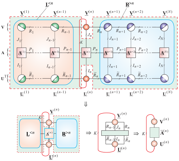
(b)

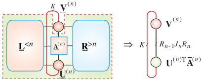
Figure 3.12: Tensor network for computing the $K$ left- and right-singular vectors corresponding to the $K$ extremal singular values. (a) This is achieved via the maximization of the trace, $\mathop{\rm tr}\nolimits({\bf U}^{\text{T}}{\bf A}{\bf V})$ or $\mathop{\rm tr}\nolimits({\bf V}^{\text{T}}{\bf A}^{\dagger}{\bf U})$, subject to the orthogonality constraints, ${\bf U}^{\text{T}}{\bf U}={\bf I}_{k}$ and ${\bf V}^{\text{T}}{\bf V}={\bf I}_{K}$. Note that the singular values are computed as ${\bf S}={\bf U}^{(n)\;\text{T}}\;\overline{\bf A}^{(n)}\,{\bf V}^{(n)}$. (b) In practice, we do not explicitly perform contraction, which leads to the matrix $\bar{\bf A}^{(n)}\in\mathbb{R}^{R_{n-1}I_{n}R_{n}\times R_{n-1}J_{n}R_{n}}$, but employ smaller matrix products ${\bf U}^{(n)\;\text{T}}\bar{\bf A}^{(n)}\in\mathbb{R}^{K\times R_{n-1}J_{n}R_{n}}$.

Similarly to the symmetric EVD problem described in the previous section, the block TT concept can be employed to compute only $K$ largest singular values and the corresponding singular vectors of a given matrix ${\bf A}\in\mathbb{R}^{I\times J}$, by performing the maximization of the following cost function [Lee and Cichocki, 2015, Cichocki, 2013, 2014]:

$$J({\bf U},{\bf V})=\mathop{\rm tr}\nolimits({\bf U}^{\text{T}}{\bf A}{\bf V}),\quad\mbox{s.t.}\quad{\bf U}^{\text{T}}{\bf U}={\bf I}_{K},\;\;{\bf V}^{\text{T}}{\bf V}={\bf I}_{K},$$ (3.40)

where ${\bf U}\in\mathbb{R}^{I\times K}$ and ${\bf V}\in\mathbb{R}^{J\times K}$.

Conversely, the computation of $K$ smallest singular values and the corresponding left and right singular vectors of a given matrix, ${\bf A}\in\mathbb{R}^{I\times J}$, can be formulated as the following optimization problem:

$$\max_{{\bf U},{\bf V}}\mathop{\rm tr}\nolimits({\bf V}^{\text{T}}{\bf A}^{\dagger}{\bf U}),\quad\mbox{s.t.}\quad{\bf U}^{\text{T}}{\bf U}={\bf I}_{K},\;\;{\bf V}^{\text{T}}{\bf V}={\bf I}_{K},$$ (3.41)

where ${\bf A}^{\dagger}\in\mathbb{R}^{J\times I}$ is the Moore-Penrose pseudo-inverse of the matrix ${\bf A}$. Now, after tensorizing the involved huge-scale matrices, an asymmetric tensor network can be constructed for the computation of $K$ extreme (minimal or maximal) singular values, as illustrated in Figure 3.12 (see [Lee and Cichocki, 2015] for detail and computer simulation experiments).

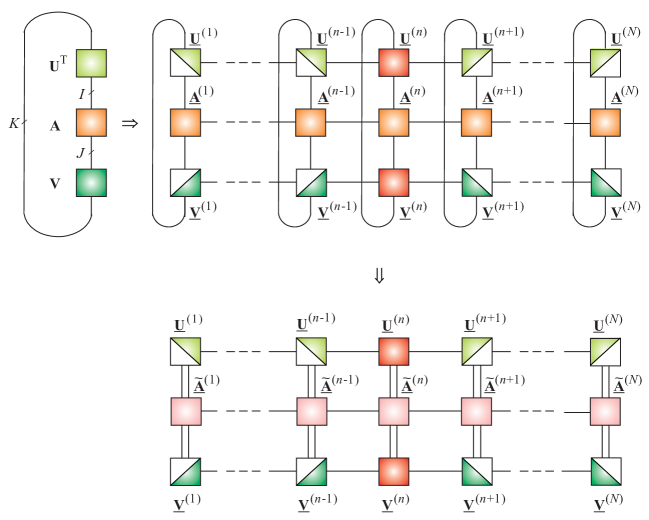
Figure 3.13: MPS/MPO tensor network with the Periodic Boundary Conditions (PBC), for the computation of a large number $K=K_{1}K_{2}\cdots K_{N}$ of extreme singular values and the corresponding left- and right-singular vectors (top). Transformation into the standard TT formats (MPS/MPO without OBC) via vectorization, with the cores $\widetilde{\bf A}^{(n)}={\bf A}^{(n)}\otimes{\bf I}$ (bottom).

The key idea behind the solutions of (3.40) and (3.41) is to perform TT core contractions to reduce the unfeasible huge-scale optimization problem to relatively small-scale optimization sub-problems, as follows:

• For the problem (3.40)

  $$\max_{{\bf U}^{(n)},{\bf V}^{(n)}}\mathop{\rm tr}\nolimits(({\bf U}^{(n)})^{\text{T}}\;\overline{\bf A}^{(n)}\;{\bf V}^{(n)}),$$ (3.42)

• For the problem (3.41)

  $$\max_{{\bf U}^{(n)},{\bf V}^{(n)}}\mathop{\rm tr}\nolimits(({\bf V}^{(n)})^{\text{T}}\;(\overline{\bf A}^{(n)})^{\dagger}\;{\bf U}^{(n)}),$$ (3.43)

subject to the orthogonality constraints

$$({\bf U}^{(n)})^{\text{T}}{\bf U}^{(n)}={\bf I}_{K},\quad({\bf V}^{(n)})^{\text{T}}{\bf V}^{(n)}={\bf I}_{K},\;\;n=1,2,\ldots,N,$$

where ${\bf U}^{(n)}\in\mathbb{R}^{\tilde{R}_{n-1}I_{n}\tilde{R}_{n}\times K}$ and ${\bf V}^{(n)}\in\mathbb{R}^{R_{n-1}J_{n}R_{n}\times K}$, while the contracted matrices are formally expressed as

$$\overline{\bf A}^{(n)}={\bf U}_{\neq n}^{\text{T}}{\bf A}{\bf V}_{\neq n}\in\mathbb{R}^{\tilde{R}_{n-1}\,I_{n}\,\tilde{R}_{n}\;\times\;R_{n-1}\,J_{n}\,R_{n}}$$ (3.44)

$$(\overline{\bf A}^{(n)})^{\dagger}={\bf V}_{\neq n}^{\text{T}}{\bf A}^{\dagger}{\bf U}_{\neq n}\in\mathbb{R}^{R_{n-1}\,J_{n}\,R_{n}\;\times\;\tilde{R}_{n-1}\,I_{n}\,\tilde{R}_{n}}.$$ (3.45)

In this way, the problem is reduced to the computation of the largest or smallest singular values of a relatively small matrix $\overline{\bf A}^{(n)}$, for which any efficient SVD algorithm can be applied.

Note that for a very large number of, say, thousands or more singular values $K=K_{1}K_{2}\cdots K_{N}$, the block-$n$ TT formats may not be efficient, and alternative tensor networks should be employed, as shown in Figure 3.13, where each TT core is a 4th-order tensor. One problem with such tensor networks with many loops is the computationally complex contraction of core tensors. However, all loops can be easily eliminated by vectorizing the orthogonal matrices

$${\bf U}\in\mathbb{R}^{I\times K}\rightarrow{\bf u}\in\mathbb{R}^{IK},\quad{\bf V}\in\mathbb{R}^{J\times K}\rightarrow{\bf u}\in\mathbb{R}^{JK}$$ (3.46)

and by rewriting the cost function as (see bottom part of Figure 3.13)

$$J({\bf U},{\bf V}) = \mathop{\rm tr}\nolimits({\bf U}^{\text{T}}{\bf A}{\bf V})\rightarrow$$

$$J({\bf u},{\bf v}) = {\bf u}^{\text{T}}\widetilde{\bf A}{\bf v}={\bf u}^{\text{T}}({\bf A}\otimes{\bf I}_{K}){\bf v},$$ (3.47)

where $\widetilde{\bf A}={\bf A}\otimes{\bf I}_{K}\in\mathbb{R}^{IK\times JK}$.

3.6 GEVD and Related Problems using TT Networks

Table 3.2 illustrates the rich scope of the Generalized Eigenvalue Decomposition (GEVD), a backbone of many standard methods for linear dimensionality reduction, classification, and clustering [Kokiopoulou et al., 2011, Cunningham and Ghahramani, 2015, Benson et al., 2015, Gleich et al., 2015, Wu et al., 2016].

Table 3.2: Cost functions and constraints used in classical feature extraction (dimensionality reduction) methods that can be formulated as the symmetric (generalized) eigenvalue problem, $\min_{{\bf V}}({\bf V}^{\text{T}}{\bf X}{\bf C}{\bf X}^{\text{T}}{\bf V})$. The objective is to find an (orthogonal) matrix, ${\bf V}$, assuming that data matrices, ${\bf X}$, ${\bf W},{\bf D},{\bf H}$, are known. The symmetric matrix ${\bf C}$ can take different forms, for example, ${\bf C}={\bf I}-\frac{1}{N}{\bf 11}^{\text{T}},\;{\bf C}={\bf D}-{\bf W},\;{\bf C}=({\bf I}-{\bf W}^{\text{T}})({\bf I}-{\bf W}),\;{\bf C}={\bf I}-{\bf H},$ depending on the method used (for more detail, see e.g. [Kokiopoulou et al., 2011, Cunningham and Ghahramani, 2015]).

Method Cost Function (min) Constraints Principal Component Analysis/Multi-Dimensional Scaling (PCA/MDS) $\mathop{\rm tr}\nolimits[-{\bf V}^{\text{T}}{\bf X}({\bf I}-\frac{1}{N}{\bf 11}^{\text{T}}){\bf X}^{\text{T}}{\bf V}]$ ${\bf V}^{\text{T}}{\bf V}={\bf I}$ Locally Preserving Projection (LPP) $\mathop{\rm tr}\nolimits[{\bf V}^{\text{T}}{\bf X}({\bf D}-{\bf W}){\bf X}^{\text{T}}{\bf V}]$ ${\bf V}^{\text{T}}{\bf XDX}^{\text{T}}{\bf V}={\bf I}$ Orthogonal LPP (OLPP) $\mathop{\rm tr}\nolimits[{\bf V}^{\text{T}}{\bf X}({\bf{D-W}}){\bf X}^{\text{T}}{\bf V}]$ ${\bf V}^{\text{T}}{\bf V}={\bf I}$ Neighborhood Preserving Projection (NPP) $\mathop{\rm tr}\nolimits[{\bf V}^{\text{T}}{\bf X}({\bf I}-{\bf W}^{\text{T}})({\bf I}-{\bf W}){\bf X}^{\text{T}}{\bf V}]$ ${\bf V}^{\text{T}}{\bf XX}^{\text{T}}{\bf V}={\bf I}$ Orthogonal NPP (ONPP) $\mathop{\rm tr}\nolimits[{\bf V}^{\text{T}}{\bf X}({\bf I}-{\bf W}^{\text{T}})({\bf I}-{\bf W}){\bf X}^{\text{T}}{\bf V}]$ ${\bf V}^{\text{T}}{\bf V}={\bf I}$ Linear Discriminant Analysis (LDA) $\mathop{\rm tr}\nolimits[{\bf V}^{\text{T}}{\bf X}({\bf I}-{\bf H}){\bf X}^{\text{T}}{\bf V}]$ ${\bf V}^{\text{T}}{\bf XX}^{\text{T}}{\bf V}={\bf I}$ Spectral Clustering (Ratio Cut) $\mathop{\rm tr}\nolimits[{\bf V}^{\text{T}}({\bf D}-{\bf W}){\bf V}]$ ${\bf V}^{\text{T}}{\bf V}={\bf I}$ Spectral Clustering (Normalized Cut) $\mathop{\rm tr}\nolimits[{\bf V}^{\text{T}}({\bf D}-{\bf W}){\bf V}]$ ${\bf V}^{\text{T}}{\bf DV}={\bf I}$

For example, the standard PCA, PLS, orthonormalized PLS (OPLS) and CCA can be formulated as the following EVD/GEVD problems

$$\mbox{PCA :}\qquad{\bf C}_{x}{\bf v}=\lambda{\bf v}$$ (3.48)

$$\mbox{OPLS :}\quad\;\;{\bf C}_{xy}{\bf C}^{\text{T}}_{xy}{\bf v}=\lambda{\bf C}_{x}{\bf v}$$ (3.49)

$$\mbox{PLS :}\qquad\left[\begin{matrix}{\bf 0}&{\bf C}_{xy}\\ {\bf C}^{\text{T}}_{xy}&{\bf 0}\end{matrix}\right]\left[\begin{matrix}{\bf v}\\ {\bf u}\end{matrix}\right]=\lambda\left[\begin{matrix}{\bf v}\\ {\bf u}\end{matrix}\right]$$ (3.50)

$$\mbox{CCA :}\quad\;\;\left[\begin{matrix}{\bf 0}&{\bf C}_{xy}\\ {\bf C}^{\text{T}}_{xy}&{\bf 0}\end{matrix}\right]\left[\begin{matrix}{\bf v}\\ {\bf u}\end{matrix}\right]=\lambda\left[\begin{matrix}{\bf C}_{x}&\mbox{\boldmath${\bf 0}$}\\ {\bf 0}&{\bf C}^{\text{T}}_{y}\end{matrix}\right]\left[\begin{matrix}{\bf v}\\ {\bf u}\end{matrix}\right],$$ (3.51)

where for given data matrices ${\bf X}$ and ${\bf Y}$, ${\bf C}_{x}={\bf X}^{\text{T}}{\bf X}$ and ${\bf C}_{y}={\bf Y}^{\text{T}}{\bf Y}$ are the sample covariance matrices, while ${\bf C}_{xy}={\bf X}^{\text{T}}{\bf Y}$ is the sample cross-covariance matrix.

In general, the GEVD problem can be formulated as the following trace optimization (maximization or minimization) problem

$$\max_{{\bf V}\in\mathbb{R}^{I\times K}}\mathop{\rm tr}\nolimits({\bf V}^{\text{T}}{\bf A}{\bf V}),\quad\mbox{s.t.}\quad{\bf V}^{\text{T}}{\bf B}{\bf V}={\bf I}_{K},$$ (3.52)

where the symmetric matrix, ${\bf A}\in\mathbb{R}^{I\times I}$, and symmetric positive-definite matrix, ${\bf B}\in\mathbb{R}^{I\times I}$, are known, while the objective is to estimate $K$ largest (or the smallest in the case of minimization) eigenvalues and the corresponding eigenvectors represented by the orthonormal matrix ${\bf V}\in\mathbb{R}^{I\times K}$, with $I=I_{1}I_{2}\cdots I_{N}$ and $K=K_{1}K_{2}\cdots K_{N}$. For the estimation of the $K$ smallest eigenvalues, the minimization of the cost function is performed instead of the maximization.

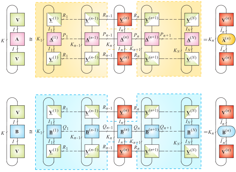
Figure 3.14: Conceptual tensor networks for trace ratio optimization in TT formats. Note that for a moderate number $K$, all the loops but one may have a dimension (size) of unity and can thus be removed.

It is sometimes more elegant to incorporate the constraint, ${\bf V}^{\text{T}}{\bf B}{\bf V}={\bf I}_{K}$, into (3.52) into the trace operator, to give the following optimization problem [Absil et al., 2008]

$$\min_{{\bf V}\in\mathbb{R}^{I\times K}}\mathop{\rm tr}\nolimits({\bf V}^{\text{T}}{\bf A}{\bf V}({\bf V}^{\text{T}}{\bf B}{\bf V})^{-1}).$$ (3.53)

or alternatively, to represent GEVD approximately as an unconstrained optimization problem

$$\min_{{\bf V}\in\mathbb{R}^{I\times K}}\mathop{\rm tr}\nolimits({\bf V}^{\text{T}}{\bf A}{\bf V})+\gamma\;\|{\bf V}^{\text{T}}{\bf B}{\bf V}-{\bf I}_{K}\|^{2}_{F},$$ (3.54)

where the parameter $\gamma>0$ controls the orthogonality level of ${\bf B}$.

Also, by a change in the variables, ${\bf W}={\bf B}^{1/2}{\bf V}$, the GEVD reduces to the standard symmetric EVD [Cunningham and Ghahramani, 2015]

$$\min_{{\bf W}\in\mathbb{R}^{I\times K}}\mathop{\rm tr}\nolimits({\bf W}^{\text{T}}{\bf B}^{-1/2}{\bf A}{\bf B}^{-1/2}{\bf W}),\;\;\mbox{s.t.}\;\;{\bf W}^{\text{T}}{\bf W}={\bf I}_{K}.$$

Finally, the GEVD is closely related but not equivalent, to the trace ratio optimization problem, given by

$$\min_{{\bf V}\in\mathbb{R}^{I\times K}}\frac{\mathop{\rm tr}\nolimits({\bf V}^{\text{T}}{\bf A}{\bf V})}{\mathop{\rm tr}\nolimits({\bf V}^{\text{T}}{\bf B}{\bf V})},\quad\mbox{s.t.}\quad{\bf V}^{\text{T}}{\bf V}={\bf I}_{K}.$$ (3.55)

Figure 3.14 illustrates the trace ratio optimization for huge-scale matrices, whereby the two TT networks represent approximately $\mathop{\rm tr}\nolimits({\bf V}^{\text{T}}{\bf A}{\bf V})$ and $\mathop{\rm tr}\nolimits({\bf V}^{\text{T}}{\bf B}{\bf V})$. These sub-networks are simultaneously optimized in the sense that one is being minimized while the other is being maximized, subject to orthogonality constraints. The objective is to estimate the matrix ${\bf V}\in\mathbb{R}^{I\times K}$ in the TT format, assuming that huge-scale structured matrices ${\bf A},{\bf B}$ and ${\bf V}$ admit good low-rank TT approximations.

Figure 3.14 illustrates that a recursive contraction of TT cores reduces the trace ratio optimization problem (3.55) to a set of following smaller scale trace ratio minimizations

$$\min_{{\bf V}^{(n)}\in\mathbb{R}^{\overline{I}_{n}\times K_{n}}}\frac{\mathop{\rm tr}\nolimits(({\bf V}^{(n)})^{\text{T}}\;\overline{\bf A}^{(n)}\;{\bf V}^{(n)})}{\mathop{\rm tr}\nolimits(({\bf V}^{(n)})^{\text{T}}\;\overline{\bf B}^{(n)}\;{\bf V}^{(n)})},\quad\mbox{s.t.}\quad({\bf V}^{(n)})^{\text{T}}{\bf V}^{(n)}={\bf I}_{K_{n}},$$

(3.56)

where the relatively small-size matrices, $\overline{\bf A}^{(n)}$ and $\overline{\bf B}^{(n)}$, are formally defined as

$$\overline{\bf A}^{(n)}=[{\bf V}_{\neq n}^{\text{T}}{\bf A}{\bf V}_{\neq n}]\in\mathbb{R}^{R_{n-1}I_{n}R_{n}\times R_{n-1}I_{n}R_{n}}$$ (3.57)

and

$$\overline{\bf B}^{(n)}=[{\bf V}_{\neq n}^{\text{T}}{\bf B}{\bf V}_{\neq n}]\in\mathbb{R}^{R_{n-1}I_{n}R_{n}\times R_{n-1}I_{n}R_{n}}.$$ (3.58)

3.6.1 TT Networks for Canonical Correlation Analysis (CCA)

The Canonical Correlation Analysis (CCA) method, introduced by Hotelling in 1936, can be considered as a generalization of the PCA, and is a classical method for determining the relationship between two sets of variables (for modern approaches to CCA, see [Bach and Jordan, 2005, Chu et al., 2013, Cunningham and Ghahramani, 2015] and references therein).

Given two zero-mean (i.e., centered) datasets, ${\bf X}\in\mathbb{R}^{I\times J}$ and ${\bf Y}\in\mathbb{R}^{L\times J}$, recorded from the same set of $J$ observations, the CCA seeks linear combinations of the latent variables in ${\bf X}$ and ${\bf Y}$ that are maximally mutually correlated. Formally, the classical CCA computes two projection vectors, ${\bf w}_{x}={\bf w}^{(1)}_{x}\in\mathbb{R}^{I}$ and ${\bf w}_{y}={\bf w}^{(1)}_{y}\in\mathbb{R}^{L}$, so as to maximize the correlation coefficient

$$\rho=\frac{{\bf w}^{\text{T}}_{x}{\bf X}{\bf Y}^{\text{T}}{\bf w}_{y}}{\sqrt{({\bf w}^{\text{T}}_{x}{\bf X}{\bf X}^{\text{T}}{\bf w}_{x})({\bf w}^{\text{T}}_{y}{\bf Y}{\bf Y}^{\text{T}}{\bf w}_{y})}}.$$ (3.59)

In a similar way, kernel CCA can be formulated by replacing the inner product of matrices by the kernel matrices, ${\bf K}_{x}\in\mathbb{R}^{J\times J}$ and ${\bf K}_{y}\in\mathbb{R}^{J\times J}$, to give

$$\rho=\max_{\mbox{\boldmath$\alpha$}_{x},\mbox{\boldmath$\alpha$}_{y}}\frac{\mbox{\boldmath$\alpha$}^{\text{T}}_{x}{\bf K}_{x}{\bf K}_{y}\mbox{\boldmath$\alpha$}_{y}}{\sqrt{(\mbox{\boldmath$\alpha$}^{\text{T}}_{x}{\bf K}_{x}{\bf K}_{x}\mbox{\boldmath$\alpha$}_{x})(\mbox{\boldmath$\alpha$}^{\text{T}}_{y}{\bf K}_{y}{\bf K}_{y}\mbox{\boldmath$\alpha$}_{y})}}.$$ (3.60)

Since the correlation coefficient $\rho$ is invariant to the scaling of the vectors ${\bf w}_{x}$ and ${\bf w}_{y}$, the standard CCA can be equivalently formulated as a constrained optimization problem

$$\max_{{\bf w}_{x},{\bf w}_{y}}{\bf w}_{x}^{\text{T}}{\bf X}{\bf Y}^{\text{T}}{\bf w}_{y}$$ (3.61)

$$\mbox{s.t.}\quad{\bf w}_{x}^{\text{T}}{\bf X}{\bf X}^{\text{T}}{\bf w}_{x}={\bf w}_{y}^{\text{T}}{\bf Y}^{\text{T}}{\bf Y}{\bf w}_{y}=1.$$

The vectors ${\bf t}_{1}={\bf X}^{\text{T}}{\bf w}_{x}$ and ${\bf u}_{1}={\bf Y}^{\text{T}}{\bf w}_{y}$ are referred to as the canonical variables.

Multiple canonical vectors for the classical CCA can be computed by reformulating the optimization problem in (3.61), as follows

$$\max_{{\bf W}_{x},\;{\bf W}_{y}}\mathop{\rm tr}\nolimits({\bf W}^{\text{T}}_{x}\;{\bf X}\;{\bf Y}^{\text{T}}\;{\bf W}_{y})$$ (3.62)

$$\mbox{s.t.}\quad{\bf W}^{\text{T}}_{x}\;{\bf X}{\bf X}^{\text{T}}\;{\bf W}_{x}={\bf I}_{K},\ {\bf W}^{\text{T}}_{y}\;{\bf Y}{\bf Y}^{\text{T}}\;{\bf W}_{y}={\bf I}_{K},\ {\bf W}^{\text{T}}_{x}\;{\bf X}{\bf Y}^{\text{T}}\;{\bf W}_{y}=\mbox{\boldmath$\Lambda$},$$

where ${\bf W}_{x}=[{\bf w}_{x}^{(1)},{\bf w}_{x}^{(2)},\ldots,{\bf w}_{x}^{(K)}]\in\mathbb{R}^{I\times K}$ and ${\bf W}_{y}=[{\bf w}_{y}^{(1)},{\bf w}_{y}^{(2)},\ldots,{\bf w}_{y}^{(K)}]\in\mathbb{R}^{L\times K}$ and $\Lambda$ is any diagonal matrix. However, this may become computationally very expensive due to orthogonality constraints for large-scale matrices.

An alternative approach is to use the orthogonal CCA model, which can be formulated as [Cunningham and Ghahramani, 2015]

$$\max_{{\bf W}_{x},{\bf W}_{y}}\left(\frac{\mathop{\rm tr}\nolimits({\bf W}^{\text{T}}_{x}{\bf X}{\bf Y}^{\text{T}}{\bf W}_{y})}{\sqrt{\mathop{\rm tr}\nolimits({\bf W}^{\text{T}}_{x}{\bf X}{\bf X}^{\text{T}}{\bf W}_{x})\mathop{\rm tr}\nolimits({\bf W}^{\text{T}}_{y}{\bf Y}{\bf Y}^{\text{T}}{\bf W}_{y})}}\right)$$ (3.63)

$$\mbox{s.t.}\quad\quad{\bf W}^{\text{T}}_{x}{\bf W}_{x}={\bf I}_{K},\quad{\bf W}^{\text{T}}_{y}{\bf W}_{y}={\bf I}_{K}.$$

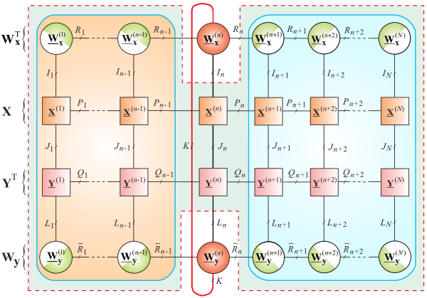
Figure 3.15: A TT sub-network for multiple orthogonal CCA components, representing in the distributed form the term $\mathop{\rm tr}\nolimits({\bf W}^{\text{T}}_{x}{\bf X}{\bf Y}^{\text{T}}{\bf W}_{y})$. Similar TT sub-networks are constructed for the normalization terms $\mathop{\rm tr}\nolimits({\bf W}^{\text{T}}_{x}{\bf X}{\bf X}^{\text{T}}{\bf W}_{x})$ and $\mathop{\rm tr}\nolimits({\bf W}^{\text{T}}_{y}{\bf Y}{\bf Y}^{\text{T}}{\bf W}_{y})$, see (3.6.1).

This model can be relatively easily implemented using the TT network approach, as illustrated in Figure 3.15. By using contractions of TT sub-networks, the huge-scale optimization problem in (3.6.1) can be transformed into a set of smaller optimization problems

$$\max_{{\bf W}^{(n)}_{x},{\bf W}^{(n)}_{y}}\left(\frac{\mathop{\rm tr}\nolimits({\bf W}^{(n)\;\text{T}}_{x}{\bf C}_{xy}^{(n)}{\bf W}^{(n)}_{y})}{\sqrt{\mathop{\rm tr}\nolimits({\bf W}^{(n)\;\text{T}}_{x}{\bf C}^{(n)}_{xx}{\bf W}_{x})\mathop{\rm tr}\nolimits({\bf W}^{(n)\;\text{T}}_{y}{\bf C}^{(n)}_{yy}{\bf W}^{(n)}_{y})}}\right)$$ (3.64)

$$\mbox{s.t.}\quad\quad{\bf W}^{(n)\;\text{T}}_{x}{\bf W}^{(n)}_{x}={\bf I}_{K},\quad{\bf W}^{(n)\;\text{T}}_{y}{\bf W}^{(n)}_{y}={\bf I}_{K},$$

for $n=1,2,\ldots,N$, where ${\bf C}^{(n)}_{xy}={\bf W}^{\text{T}}_{x,\;\neq n}{\bf X}{\bf Y}^{\text{T}}{\bf W}_{y,\;\neq n}$, $\;{\bf C}^{(n)}_{xx}={\bf W}^{\text{T}}_{x,\;\neq n}{\bf X}{\bf X}^{\text{T}}{\bf W}_{x,\;\neq n}$ and ${\bf C}^{(n)}_{yy}={\bf W}^{\text{T}}_{y,\;\neq n}{\bf Y}{\bf Y}^{\text{T}}{\bf W}_{y,\;\neq n}$.

For computational tractability of huge-scale CCA problems and for physical interpretability of latent variables, it is often useful to impose sparsity constraints, to yield the sparse CCA. Sparsity constraints can be imposed, for example, by applying the $\ell_{1}$-norm penalty terms to the matrices ${\bf W}_{x}$ and ${\bf W}_{y}$, and assuming that the cross-product matrices ${\bf X}{\bf X}^{\text{T}}$ and ${\bf Y}{\bf Y}^{\text{T}}$ can be roughly approximated by identity matrices [Witten et al., 2009, Witten, 2010]. Under such assumptions, a simplified optimization problem can be formulated as

$$\min_{{\bf W}_{x},{\bf w}_{y}}\left(-\mathop{\rm tr}\nolimits({\bf W}_{x}^{\text{T}}{\bf X}{\bf Y}^{\text{T}}{\bf W}_{y})+\gamma_{1}\|{\bf W}_{x}\|_{1}+\gamma_{2}\|{\bf W}_{y}\|_{1}\right)$$ (3.65)

$$\mbox{s.t.}\quad({\bf W}_{x})^{\text{T}}\;{\bf W}_{x}={\bf I}_{K}\quad({\bf W}_{y})^{\text{T}}\;{\bf W}_{y}={\bf I}_{K}.$$

A basic optimization scheme for an approximate huge sparse CCA in the TT format is illustrated in Figure 3.15, whereby the recursive contraction of TT networks reduces the problem to a set of smaller-dimensional sparse CCA problems in the forms

$$\min_{{\bf W}^{(n)}_{x},{\bf W}^{(n)}_{y}}\left(-\mathop{\rm tr}\nolimits(({\bf W}_{x}^{(n)})^{\text{T}}\;{\bf C}^{(n)}_{xy}\;{\bf W}^{(n)}_{y})+\gamma_{1}\;\|{\bf W}_{x}^{(n)}\|_{1}+\gamma_{2}\;\|{\bf W}_{y}^{(n)}\|_{1}\right)$$

(3.66)

$$\mbox{s.t.}\;\;({\bf W}_{x}^{(n)})^{\text{T}}\;{\bf W}^{(n)}_{x}={\bf I}_{K}\quad({\bf W}_{y}^{(n)})^{\text{T}}\;{\bf W}^{(n)}_{y}={\bf I}_{K},$$

for $n=1,2,\ldots,N$, where ${\bf C}^{(n)}_{xy}={\bf W}^{\text{T}}_{x,\;\neq n}{\bf X}{\bf Y}^{\text{T}}{\bf W}_{y,\;\neq n}$ are the contracted cross-covariance matrices.

Note that in the TT/MPO format, the sparsification penalty terms can be expressed as the $\ell_{1}$ norm $\|{\bf W}\|_{1}$, e.g., as a sum of $\ell_{1}$ norms of fibers of each TT-core, $\sum_{n=1}^{N}\sum_{r_{n-1},r_{n,k}}^{R_{N-1},R_{N},K}\|{\bf w}_{r_{n-1},r_{n}}^{(n,k)}\|_{1}$, or equivalently as a sum of the $\ell_{1}$ norms of slices, $\sum_{n=1}^{N}\|{\bf W}_{(2)}^{(n)}\|_{1}$ (see Section 3.8.4 for more detail). In such cases, the orthogonalization of TT cores is replaced by a simple normalization of fibers to unit length.

3.6.2 Tensor CCA for Multiview Data

The standard matrix CCA model has been generalized to tensor CCA, which in its simplest form can be formulated as the following optimization problem

$$\max_{\{{\bf w}^{(n)}\}}(\underline{{{\bf C}}}\;\bar{\times}_{1}\;{\bf w}^{(1)}\;\bar{\times}_{2}\;{\bf w}^{(2)}\;\cdots\bar{\times}_{N}\;{\bf w}^{(N)})$$ (3.67)

$$\mbox{s.t.}\qquad{\bf w}^{(n)\;\text{T}}\;{\bf C}_{nn}\;{\bf w}^{(n)}=1\qquad(n=1,2,\ldots,N),$$

where ${\bf w}^{(n)}\in\mathbb{R}^{I_{n}}$ are canonical vectors, ${\bf C}_{nn}\in\mathbb{R}^{I_{n}\times I_{n}}$ are covariance matrices and $\underline{{\bf C}}\in\mathbb{R}^{I_{1}\times I_{2}\times\cdots\times I_{N}}$ is an $N$th-order data tensor [Kim et al., 2007, Kim and Cipolla, 2009, Luo et al., 2015b].

Similar to the standard CCA, the objective is to find the canonical vectors which maximize the correlation function in (3.67). Depending on the application, the matrices ${\bf C}_{nn}$ and tensor $\underline{{\bf C}}$ can be constructed in many different ways. For example, for multi-view data with $N$ different views $\{{\bf X}_{n}\}_{n=1}^{N}$, expressed as ${\bf X}_{n}=[{\bf x}_{n1},{\bf x}_{n2},\ldots,{\bf x}_{nJ}]\in\mathbb{R}^{I_{n}\times J}$, the following sampled covariance matrices and the tensor can be constructed as [Luo et al., 2015b]

$${\bf C}_{nn} = \frac{1}{J}\sum_{j=1}^{J}({\bf x}_{nj}{\bf x}^{\text{T}}_{nj})=\frac{1}{J}{\bf X}_{n}{\bf X}_{n}^{\text{T}},$$ (3.68)

$$\underline{{\bf C}} = \frac{1}{J}\sum_{j=1}^{J}({\bf x}_{1j}\circ{\bf x}_{2j}\circ\cdots\circ{\bf x}_{Nj}).$$ (3.69)

Then the normalized data tensor, $\underline{{\bf C}}$, can be expressed as

$$\underline{\widehat{{\bf C}}}=\underline{{\bf C}}\;\times_{1}\;\widehat{{\bf C}}^{-1/2}_{11}\;\times_{2}\;\widehat{{\bf C}}^{-1/2}_{22}\;\cdots\times_{N}\;\widehat{{\bf C}}^{-1/2}_{NN}$$ (3.70)

where the regularized covariance matrices are expressed as $\widehat{{\bf C}}_{nn}={\bf C}_{nn}+\varepsilon{\bf I}_{I_{n}}$, with small regularization parameters $\varepsilon>0$ (see Figure 3.16(a)).

(a)

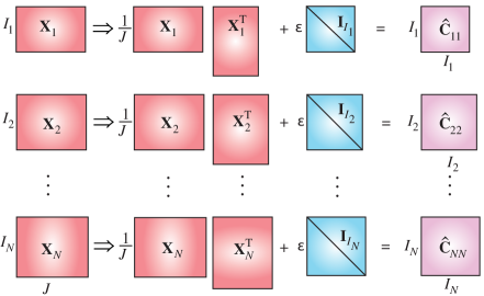
(b)

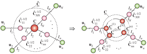
Figure 3.16: Illustration of the computation of the tensor CCA for multi-view datasets. (a) Construction of regularized covariance matrices $\widehat{{\bf C}}_{nn}=(1/J){\bf X}_{n}{\bf X}_{n}^{\text{T}}+\varepsilon{\bf I}_{I_{n}}$. (b) Distributed representation of the cost function (3.6.2) via tensor chain.

In order to find canonical vectors, the optimization problem (3.67) can be reformulated in a simplified form as

$$\max_{\{{\bf u}^{(n)}\}}\ (\underline{\widehat{{\bf C}}}\;\bar{\times}_{1}\;{\bf u}^{(1)}\;\bar{\times}_{2}\;{\bf u}^{(2)}\;\cdots\bar{\times}_{N}\;{\bf u}^{(N)})$$ (3.71)

$$\mbox{s.t.}\qquad{\bf u}^{(n)\;\text{T}}\;{\bf u}^{(n)}=1\qquad(n=1,2,\ldots,N),$$

where ${\bf u}^{(n)}=\widehat{{\bf C}}^{-1/2}_{nn}\;{\bf w}^{(n)}$, as illustrated in Figure 3.16(b).

Note that the problem is equivalent to finding the rank-one approximation, for which many efficient algorithms exist. However, if the number of views is relatively large ($N>5$) the core tensor becomes too large and we need to represent the core tensor in a distributed tensor network format (e.g., in TC format, as illustrated in Figure 3.16(b)).

3.7 Two-Way Component Analysis in TT Formats

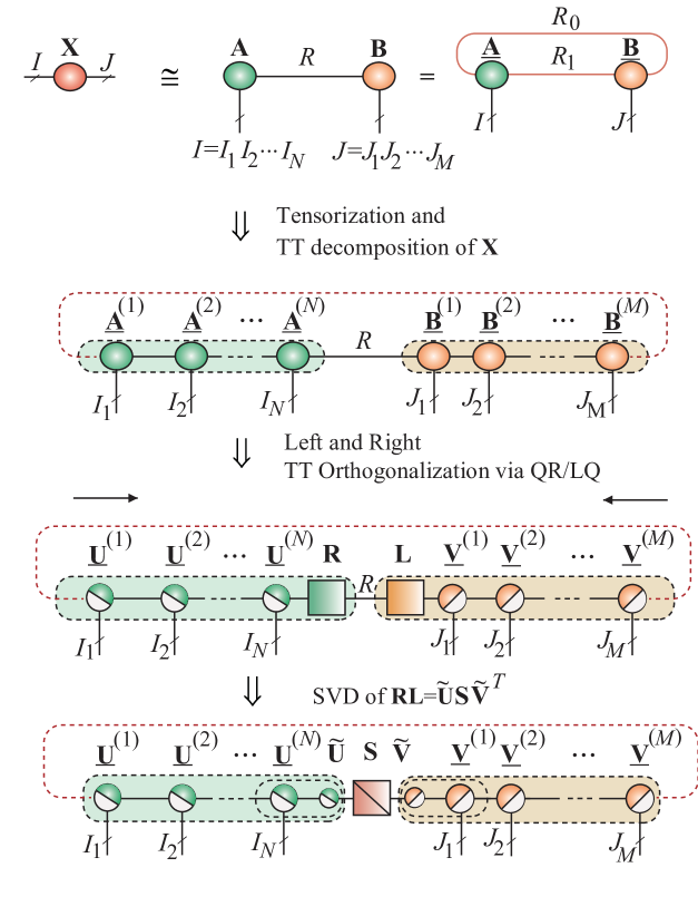
Figure 3.17: Constrained low-rank matrix factorization (LRMF), ${\bf X}\cong{\bf A}{\bf B}^{\text{T}}$, for a huge-scale structured matrix, ${\bf X}\in\mathbb{R}^{I\times J}$, in the TT/TC format (i.e., MPS with OBC or PBC). By imposing suitable orthogonality constraints on core tensors, large-scale SVD/EVD can be performed in the TT/TC format. Other constraints, such as nonnegativity and/or sparsity, are also conceptually possible.

Low-rank matrix factorizations with specific constraints can be formulated in the following standard optimization setting [Cichocki et al., 1995, Cichocki and Zdunek, 2006, 2007, Cichocki et al., 2009, Cichocki, 2011]

$$\min_{{\bf A},{\bf B}}\,J({\bf A},{\bf B})=\|{\bf X}-{\bf A}{\bf B}^{\text{T}}\|_{F}^{2},$$ (3.72)

where a large-scale data matrix, ${\bf X}\in\mathbb{R}^{I\times J}$, is given and the objective is to estimate the factor matrices, ${\bf A}\in\mathbb{R}^{I\times R}$ and ${\bf B}\in\mathbb{R}^{J\times R}$ (with the assumption that $R\ll\{I,J\}$), subject to suitable constraints being imposed on one or both factor matrices.

If such a structured data matrix can be represented by a low-rank TT or TC network (e.g., through a cheap matrix cross-approximation the factor matrices can be represented in a TT/TC format, as illustrated in the top panel of Figure 3.17), then in the first step no constraint on the TT core tensors, $\underline{{\bf A}}^{(n)}$ and $\underline{{\bf B}}^{(m)}$, need to be imposed to represent ${\bf X}$ in a distributed form. However, such a factorization is not unique and the so obtained components (in TT format) do not have any physical meaning.

With a matrix ${\bf X}$ already in a compressed TT format, in the second step, we may impose the desired constraints. For example, by imposing the left-orthogonality on TT cores of $\underline{{\bf A}}\in\mathbb{R}^{I_{1}\times\cdots\times I_{N}\times R}$ and right-orthogonality on the TT cores of $\underline{{\bf B}}\in\mathbb{R}^{R\times J_{1}\times\cdots\times J_{N}}$, a truncated SVD can be computed for the $R$ largest singular values and the corresponding singular vectors, as illustrated in the bottom panel of Figure 3.17. In a similar way, we can compute the pseudo-inverse of a huge matrix.

3.8 Solving Huge-Scale Systems of Linear Equations

Solving linear systems of large scale equations arises throughout science and engineering; e.g, convex optimization, signal processing, finite elements and machine learning all rely partially on approximately solving linear equations, typically using some additional criteria like sparseness or smoothes.

Consider a huge system of linear algebraic equations in a TT format (see also Part 1 [Cichocki et al., 2016]), given by

$${\bf A}{\bf x}\cong{\bf b}$$ (3.73)

where ${\bf A}\in\mathbb{R}^{I\times J}$, ${\bf b}\in\mathbb{R}^{I}$ and ${\bf x}\in\mathbb{R}^{J}$. The objective is to find an approximative solution, ${\bf x}\in\mathbb{R}^{J}$, in a TT format, by imposing additional constraints (regularization terms) such as smoothness, sparseness and/or nonnegativity on the vector ${\bf x}$. Several innovative TT/HT network solutions to this problem do exist (see [Oseledets and Dolgov, 2012, Dolgov and Savostyanov, 2014] and references therein), however, most focus on only symmetric square matrices. We shall next consider several more general cases.

3.8.1 Solutions for a Large-scale Linear Least Squares Problem using ALS

The Least Squares (LS) solution (often called the ridge regression) minimizes the following regularized cost function

$$J({\bf x}) = \|{\bf A}{\bf x}-{\bf b}\|^{2}_{2}+\gamma\|{\bf L}{\bf x}\|^{2}_{2}$$ (3.74)

$$= {\bf x}^{\text{T}}{\bf A}^{\text{T}}{\bf A}{\bf x}-2{\bf x}^{\text{T}}{\bf A}^{\text{T}}{\bf b}+{\bf b}^{\text{T}}{\bf b}+\gamma{\bf x}^{\text{T}}{\bf L}^{\text{T}}{\bf L}{\bf x},$$

with the Tikhonov regularization term on the right hand side, while ${\bf L}$ is the so-called smoothing matrix, typically in the form of the discrete first-order or second-order derivative matrix, and $\widetilde{\bf L}={\bf L}^{\text{T}}{\bf L}\in\mathbb{R}^{J\times J}$.

Upon neglecting the constant factor, ${\bf b}^{\text{T}}{\bf b}$, we arrive at a simplified form

$$J({\bf x})={\bf x}^{\text{T}}{\bf A}^{\text{T}}{\bf A}{\bf x}-2{\bf x}^{\text{T}}{\bf A}^{\text{T}}{\bf b}+\gamma{\bf x}^{\text{T}}\widetilde{\bf L}{\bf x}.$$ (3.75)

The approximative TT representation of the matrix ${\bf A}$ and vectors ${\bf x}$ and ${\bf b}$ allows for the construction of three tensor sub-networks, as shown in Figure 3.18. Upon simultaneous recursive contractions of all the three sub-networks for each node $n=1,2,\ldots,N$, a large-scale infeasible optimization problem in (3.74) can be converted into a set of much smaller optimization problems based on the minimization of cost functions

$$J({\bf x}) = J({\bf X}_{\neq n}{\bf x}^{(n)})$$

$$= ({\bf x}^{(n)})^{\text{T}}{\bf X}_{\neq n}^{\text{T}}{\bf A}^{\text{T}}{\bf A}{\bf X}_{\neq n}{\bf x}^{(n)}-2({\bf x}^{(n)})^{\text{T}}{\bf X}_{\neq n}^{\text{T}}{\bf A}^{\text{T}}{\bf b}$$

$$+\gamma({\bf x}^{(n)})^{\text{T}}{\bf X}_{\neq n}^{\text{T}}{\bf L}^{\text{T}}{\bf L}{\bf X}_{\neq n}{\bf x}^{(n)},\quad n=1,2,\ldots,N.$$

These can be expressed in the following equivalent compact forms

$$J_{n}({\bf x}^{(n)})=({\bf x}^{(n)})^{\text{T}}\;\overline{\bf A}^{(n)}\,{\bf x}^{(n)}-2({\bf x}^{(n)})^{\text{T}}\;\overline{\bf b}^{(n)}+\gamma({\bf x}^{(n)})^{\text{T}}\;\overline{\bf L}^{(n)}\,{\bf x}^{(n)}.$$

(3.77)

where ${\bf x}^{(n)}\in\mathbb{R}^{R_{n-1}J_{n}R_{n}}$, $\overline{\bf A}^{(n)}={\bf X}_{\neq n}^{\text{T}}{\bf A}^{\text{T}}{\bf A}{\bf X}_{\neq n}\in\mathbb{R}^{R_{n-1}J_{n}R_{n}\times R_{n-1}J_{n}R_{n}}$, $\overline{\bf b}^{(n)}={\bf X}_{\neq n}^{\text{T}}{\bf A}^{\text{T}}{\bf b}\in\mathbb{R}^{R_{n-1}J_{n}R_{n}}$, and $\overline{\bf L}^{(n)}={\bf X}_{\neq n}^{\text{T}}{\bf L}^{\text{T}}{\bf L}{\bf X}_{\neq n}\in\mathbb{R}^{R_{n-1}J_{n}R_{n}\times R_{n-1}J_{n}R_{n}}$.

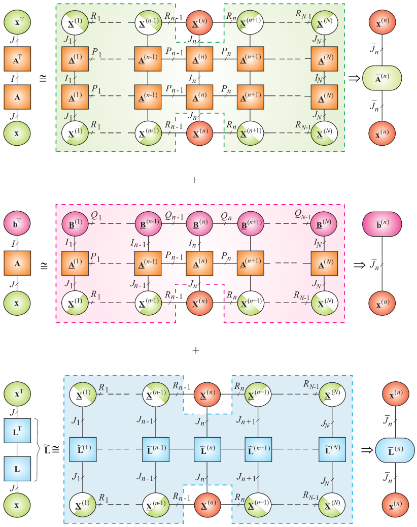
Figure 3.18: A TT network, consisting of three sub-networks, which solves (in the LS sense) a system of linear equations in the form ${\bf A}{\bf x}\approx{\bf b}$, where ${\bf A}\in\mathbb{R}^{I_{1}\cdots I_{N}\;\times\;J_{1}\cdots J_{N}}$ is a huge non-symmetric matrix and the Tikhonov regularized cost function is expressed as $J({\bf x})=\|{\bf A}{\bf x}-{\bf b}\|_{2}^{2}+\gamma\|{\bf L}{\bf x}\|^{2}_{2}={\bf x}^{\text{T}}{\bf A}^{\text{T}}{\bf A}{\bf x}-2{\bf b}^{\text{T}}{\bf A}{\bf x}+{\bf b}^{\text{T}}{\bf b}+\gamma{\bf x}^{\text{T}}{\bf L}^{\text{T}}{\bf L}{\bf x}$.

In this way, a large-scale system of linear equations is converted into a set of smaller-size systems, which can be solved by any standard method

$$\overline{\bf A}^{(n)}\,{\bf x}^{(n)}\cong\overline{\bf b}^{(n)},\qquad n=1,2,\ldots,N,$$ (3.78)

It is important to note that if the TT cores are left- and right-orthonormalized, the symmetric semi-positive definite matrix $\overline{\bf A}^{(n)}$ is better conditioned than the original huge matrix ${\bf A}$.

The matrix multiplications in (3.77) is not performed explicitly, however, the TT format alleviates the curse of dimensionality via a recursive contraction of cores, as shown in Figure 3.18.

Remark. The usual assumption that all data admits low-rank TT/QTT approximations is a key condition for successfully employing this approach. However, for data with a weak structure, TT approximations may have relatively large ranks which makes the calculation difficult or even impossible. The way in which the TT ranks are chosen and adapted is therefore the key factor in efficiently solving huge-scale structured linear systems.

3.8.2 Alternating Minimum Energy (AMEn) Algorithm for Solving a Large-scale Linear Least Squares Problems

The AMEn approach, introduced in Section 3.4.4 for the EVD problem, has been developed first historically as an efficient solution to large-scale least squares problems [Dolgov and Savostyanov, 2014]. The main difference from the EVAMEn method for solving eigenvalue problems is in the definition of the gradient of the cost function and in the computation of enrichment cores $\underline{{\bf Z}}^{(n)}$.

Algorithm 12 summarizes the AMEn algorithm for solving huge systems of linear equations ${\bf A}{\bf x}\cong{\bf b}$, for ${\bf A}\in\mathbb{R}^{I\times J}$ and ${\bf b}\in\mathbb{R}^{I}$ given in the TT format, with $I=I_{1}I_{2}\cdots I_{N}$ and $J=J_{1}J_{2}\cdots J_{N}$. In the first preliminary step, we assume, that the core $\underline{{\bf X}}^{(n)}\in\mathbb{R}^{R_{n-1}\times J_{n}\times R_{n}}$ has been updated at the $n$th micro-iteration by solving the reduced linear system $\overline{\bf A}^{(n)}\,{\bf x}^{(n)}\cong\overline{\bf b}^{(n)}$, similarly to the ALS method described in the previous section. Note that solving this reduced linear system is equivalent to minimizing the cost function $J({\bf x})=\|{\bf A}{\bf x}-{\bf b}\|^{2}$ with respect to the core ${\bf X}^{(n)}$. Similarly, for a residual vector defined as $\widetilde{{\bf r}}={\bf A}^{\text{T}}({\bf A}{\bf x}-{\bf b})\in\mathbb{R}^{J}$ in the TT format (i.e., $\underline{\widetilde{{\bf R}}}=\mathopen{\hbox{\set@color${\langle}$}\kern-1.94444pt\leavevmode\hbox{\set@color${\langle}$}}\underline{\widetilde{{\bf R}}}^{(1)},\underline{\widetilde{{\bf R}}}^{(2)},\ldots,\underline{\widetilde{{\bf R}}}^{(N)},\mathclose{\hbox{\set@color${\rangle}$}\kern-1.94444pt\leavevmode\hbox{\set@color${\rangle}$}}$, each of its TT cores $\underline{\widetilde{{\bf R}}}^{(n)}\in\mathbb{R}^{Q_{n-1}\times J_{n}\times Q_{n}}$ can be updated via the ALS scheme by $\widetilde{{\bf r}}^{(n)}={\bf R}_{\neq n}^{\text{T}}\;\widetilde{{\bf r}}=\arg\min_{\underline{\widetilde{{\bf R}}}^{(n)}}\|\widetilde{{\bf r}}-({\bf A}^{\text{T}}{\bf A}{\bf x}-{\bf A}^{\text{T}}{\bf b})\|^{2}$. In other words, the vector $\widetilde{{\bf r}}$ approximates the gradient vector, $\nabla J({\bf x})\propto{\bf A}^{\text{T}}{\bf A}{\bf x}-{\bf A}^{\text{T}}{\bf b}$, and it can be efficiently updated via the contractions of core tensors.

0:  Matrix ${\bf A}\in\mathbb{R}^{I\times J}$, with $I\geq J$, vector ${\bf b}\in\mathbb{R}^{I}$, initial

guesses for ${\bf x}\in\mathbb{R}^{J}$ and residual $\widehat{{\bf r}}={\bf A}^{\text{T}}({\bf A}{\bf x}-{\bf b})\in\mathbb{R}^{J}$ in the

TT format

0:  Approximate solution ${\bf x}$ in the TT format $\underline{{\bf X}}=\mathopen{\hbox{\set@color${\langle}$}\kern-1.94444pt\leavevmode\hbox{\set@color${\langle}$}}\underline{{\bf X}}^{(1)},\underline{{\bf X}}^{(2)},\ldots,\underline{{\bf X}}^{(N)}\mathclose{\hbox{\set@color${\rangle}$}\kern-1.94444pt\leavevmode\hbox{\set@color${\rangle}$}}$

1:  while not converged or iteration limit is not reached do

2:     Right-orthogonalize cores $\underline{{\bf X}}^{(n)},\underline{\widehat{{\bf R}}}^{(n)}$ for $n=N,N-1,\ldots,2$

3:     for $n=1$ to $N$ do

4:        Update the core $\underline{{\bf X}}^{(n)}$ by solving $\overline{\bf A}^{(n)}\,{\bf x}^{(n)}\cong\overline{\bf b}^{(n)}$

5:        Update the core $\underline{\widehat{{\bf R}}}^{(n)}$ by solving ${\bf R}_{\neq n}\widehat{{\bf r}}^{(n)}\cong\widehat{{\bf r}}$

6:        if $n<N$ then

7:           Compute the core $\underline{{\bf Z}}^{(n)}$ of the partially projected

gradient by solving $({\bf X}^{<n}\otimes_{L}{\bf I}_{J_{n}}\otimes_{L}({\bf R}^{>n})^{\text{T}})\;{\bf z}^{(n)}\cong\widehat{{\bf r}}$

8:           Enrich the cores ${\bf X}^{(n)}_{j_{n}}\leftarrow[{\bf X}^{(n)}_{j_{n}},\;{\bf Z}^{(n)}_{j_{n}}]$ and ${\bf X}^{(n+1)}_{j_{n+1}}\leftarrow\left[\begin{matrix}{\bf X}^{(n+1)}_{j_{n+1}}\\ {\bf 0}\end{matrix}\right]$

9:           Left-orthogonalize cores $\underline{{\bf X}}^{(n)},\underline{{\bf R}}^{(n)}$

10:        end if

11:     end for

12:  end while

13:  return  $\underline{{\bf X}}=\mathopen{\hbox{\set@color${\langle}$}\kern-1.94444pt\leavevmode\hbox{\set@color${\langle}$}}\underline{{\bf X}}^{(1)},\underline{{\bf X}}^{(2)},\ldots,\underline{{\bf X}}^{(N)}\mathclose{\hbox{\set@color${\rangle}$}\kern-1.94444pt\leavevmode\hbox{\set@color${\rangle}$}}$

Algorithm 12 AMEn for linear systems ${\bf A}{\bf x}\cong{\bf b}$ [Dolgov and Savostyanov, 2014]

Next, for building an enrichment, $\underline{{\bf Z}}^{(n)}\in\mathbb{R}^{R_{n-1}\times J_{n}\times Q_{n}}$, [Dolgov and Savostyanov, 2014] considered an approximation to the partially projected gradient

$$({\bf X}^{<n}\otimes_{L}{\bf I}_{J_{n}\cdots J_{N}})^{\text{T}}({\bf A}^{\text{T}}{\bf A}{\bf x}-{\bf A}^{\text{T}}{\bf b})\\ \cong\text{vec}\left(\mathopen{\hbox{\set@color${\langle}$}\kern-1.94444pt\leavevmode\hbox{\set@color${\langle}$}}\underline{{\bf Z}}^{(n)},\underline{{\bf R}}^{(n+1)},\ldots,\underline{{\bf R}}^{(N)}\mathclose{\hbox{\set@color${\rangle}$}\kern-1.94444pt\leavevmode\hbox{\set@color${\rangle}$}}\right)\in\mathbb{R}^{R_{n-1}J_{n}\cdots J_{N}}$$ (3.79)

with respect to $\underline{{\bf Z}}^{(n)}$ in the TT format. Since $\text{vec}(\mathopen{\hbox{\set@color${\langle}$}\kern-1.94444pt\leavevmode\hbox{\set@color${\langle}$}}\underline{{\bf Z}}^{(n)},\underline{{\bf R}}^{(n+1)},\ldots,\underline{{\bf R}}^{(N)}\mathclose{\hbox{\set@color${\rangle}$}\kern-1.94444pt\leavevmode\hbox{\set@color${\rangle}$}})=({\bf I}_{R_{n-1}J_{n}}\otimes_{L}({\bf R}^{>n})^{\text{T}})\;{\bf z}^{(n)},$ the following closed form representation can be obtained

$${\bf z}^{(n)}=({\bf X}^{<n}\otimes_{L}{\bf I}_{J_{n}}\otimes_{L}({\bf R}^{>n})^{\text{T}})^{\text{T}}\;{\bf r}$$ (3.80)

which can be efficiently computed via recursive contractions of core tensors, similarly to the standard ALS method.

Note that due to the partial gradient projection, the sizes of the TT cores $\underline{{\bf X}}^{(n)}$ and $\underline{{\bf Z}}^{(n)}$ now become consistent, which allows us to perform the concatenation

$$\widetilde{\underline{{\bf X}}}^{(n)}\leftarrow\underline{{\bf X}}^{(n)}\boxplus_{\;3}\underline{{\bf Z}}^{(n)}\in\mathbb{R}^{R_{n-1}\times J_{n}\times(R_{n}+Q_{n})},$$ (3.81)

or equivalently, $\widetilde{{\bf X}}^{(n)}_{j_{n}}\leftarrow[{\bf X}^{(n)}_{j_{n}},\;{\bf Z}^{(n)}_{j_{n}}]\in\mathbb{R}^{R_{n-1}\times(R_{n}+Q_{n})}$.

After the enrichment and the subsequent orthogonalization of the TT cores, the column space (i.e., the subspace spanned by the columns) of the frame matrix, say ${\bf X}_{\neq n+1}$, is expanded (see [Kressner et al., 2014a] for more detail).

For rigor, it can be shown that

$$\text{range}\left(\widehat{\bf X}_{\neq n+1}\right)\supset\text{range}\left({\bf X}_{\neq n+1}\right),$$

where $\text{range}({\bf A})$ denotes the column space of a matrix ${\bf A}$, whereas ${\bf X}_{\neq n+1}$ and $\widehat{\bf X}_{\neq n+1}$ are the frame matrices before and after the enrichment and orthogonalization. It should be noted that $\text{range}({\bf X}_{\neq n+1})=\text{range}({\bf X}^{<n+1})\otimes\mathbb{R}^{J_{n+1}}\otimes\text{range}(({\bf X}^{>n+1})^{\text{T}})$, and that ${\bf X}^{<n+1}=\left({\bf X}^{<n}\otimes_{L}{\bf I}_{J_{n}}\right){\bf X}^{(n)}_{L}\in\mathbb{R}^{J_{1}J_{2}\cdots J_{n}\times R_{n}},$ where ${\bf X}^{(n)}_{L}$ is the left unfolding of $\underline{{\bf X}}^{(n)}$. The left-orthogonalization of the enriched core $\widetilde{\underline{{\bf X}}}^{(n)}$ in (3.81) can be written as

$$\widetilde{\bf X}^{(n)}_{L}=\begin{bmatrix}{\bf X}^{(n)}_{L}&{\bf Z}^{(n)}_{L}\end{bmatrix}=\widehat{\bf X}^{(n)}_{L}{\bf P}\in\mathbb{R}^{R_{n-1}J_{n}\times(R_{n}+Q_{n})},$$

where $\widehat{\underline{{\bf X}}}^{(n)}\in\mathbb{R}^{R_{n-1}\times J_{n}\times\hat{R}_{n}}$ is the left-orthogonalized core and ${\bf P}\in\mathbb{R}^{\hat{R}_{n}\times(R_{n}+Q_{n})}$ is a full row rank matrix. From these expressions, it follows that $\text{range}(\widehat{\bf X}^{<n+1})\supset\text{range}({\bf X}^{<n+1})$.

3.8.3 Multivariate Linear Regression and Regularized Approximate Estimation of Moore-Penrose Pseudo-Inverse

The approaches described in the two previous sections can be straightforwardly extended to regularized multivariate regression, which can be formulated in a standard way as the minimization of the cost function

$$J({\bf X}) = \|{\bf A}{\bf X}-{\bf B}\|^{2}_{F}+\gamma\|{\bf L}{\bf X}\|^{2}_{F}$$

$$= \mathop{\rm tr}\nolimits({\bf X}^{\text{T}}{\bf A}^{\text{T}}{\bf A}{\bf X})-2\mathop{\rm tr}\nolimits({\bf B}^{\text{T}}{\bf A}{\bf X})+\mathop{\rm tr}\nolimits({\bf B}^{\text{T}}{\bf B})+\gamma\mathop{\rm tr}\nolimits({\bf X}^{\text{T}}{\bf L}^{\text{T}}{\bf L}{\bf X}),$$

where ${\bf A}\in\mathbb{R}^{I\times J}$ (with $I\geq J$), ${\bf B}\in\mathbb{R}^{I\times K}$, ${\bf X}\in\mathbb{R}^{J\times K}$ and ${\bf L}\in\mathbb{R}^{J\times J}$ (see Figure 3.19). The objective is to find an approximative solution, ${\bf X}\in\mathbb{R}^{J\times K}$, in a TT format, by imposing additional constraints (e.g., via Tikhonov regularization). In a special case when ${\bf B}={\bf I}_{I}$, for $K=I$ the problem is equivalent to the computation of Moore-Penrose pseudo inverse in an appropriate TT format (see [Lee and Cichocki, 2016b] for computer simulation experiments).

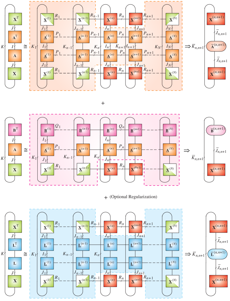
Figure 3.19: TT sub-networks for the minimization of a very large-scale regularized cost function $J({\bf X})=\|{\bf A}{\bf X}-{\bf B}\|_{F}^{2}+\gamma\|{\bf L}{\bf X}\|^{2}_{F}=\mathop{\rm tr}\nolimits({\bf X}^{\text{T}}{\bf A}^{\text{T}}{\bf A}{\bf X})-2\mathop{\rm tr}\nolimits({\bf B}^{\text{T}}{\bf A}{\bf X})+\gamma\mathop{\rm tr}\nolimits({\bf X}^{\text{T}}{\bf L}^{\text{T}}{\bf L}{\bf X})+\mathop{\rm tr}\nolimits({\bf B}^{\text{T}}{\bf B})$. This is achieved by contractions of core tensors using the MALS (DMRG2) approach. These contractions convert the huge-scale cost function to relatively smaller-scale cost functions. The top panel represents the cost function $\mathop{\rm tr}\nolimits({\bf X}^{\text{T}}{\bf A}^{\text{T}}{\bf A}{\bf X})$, the middle panel describes the cost function $\mathop{\rm tr}\nolimits({\bf B}^{\text{T}}{\bf A}{\bf X})$, while the bottom panel represents regularization term $\mathop{\rm tr}\nolimits({\bf X}^{\text{T}}{\bf L}^{\text{T}}{\bf L}{\bf X})$.

The approximative TT representation of matrices ${\bf A}$, ${\bf B}$ and ${\bf X}$ generates TT sub-networks shown in Figure 3.19, which can be optimized by the ALS or MALS (DMRG2) approaches.

By minimizing all three sub-networks simultaneously using recursive contractions of TT cores and performing ALS sequentially for each node $n=1,2,\ldots,N$, a large-scale infeasible optimization problem in (3.8.3) can be converted into a set of much smaller optimization problems expressed by the set of (linked) cost functions

$$J_{n}({\bf X}^{(n)}) = \mathop{\rm tr}\nolimits\left(({\bf X}^{(n)})^{\text{T}}\;\overline{\bf A}^{(n)}\,{\bf X}^{(n)}\right)-2\mathop{\rm tr}\nolimits\left((\overline{\bf B}^{(n)})^{\text{T}}\,{\bf X}^{(n)}\right)+$$ (3.83)

$$+\gamma\mathop{\rm tr}\nolimits\left(({\bf X}^{(n)})^{\text{T}}\;\overline{\bf L}^{(n)}\,{\bf X}^{(n)}\right),\;\;n=1,\ldots,N,$$

where

$$\overline{\bf A}^{(n)} = {\bf X}_{\neq n}^{\text{T}}{\bf A}^{\text{T}}{\bf A}{\bf X}_{\neq n}\in\mathbb{R}^{\overline{J}_{n}\times\overline{J}_{n}},$$

$$\overline{\bf B}^{(n)} = {\bf X}_{\neq n}^{\text{T}}{\bf A}^{\text{T}}{\bf B}\in\mathbb{R}^{\overline{J}_{n}\times\overline{K}_{n}},$$

$$\overline{\bf L}^{(n)} = {\bf X}_{\neq n}^{\text{T}}{\bf L}^{\text{T}}{\bf L}{\bf X}_{\neq n}\in\mathbb{R}^{\overline{J}_{n}\times\overline{J}_{n}}$$

and ${\bf X}^{(n)}\in\mathbb{R}^{\overline{J}_{n}\times\overline{K}_{n}}$, with $\overline{J}_{n}=R_{n-1}J_{n}R_{n}$ and $\overline{K}_{n}=R_{n-1}K_{n}R_{n}$.

The regularization term, $\gamma\mathop{\rm tr}\nolimits\left(({\bf X}^{(n)})^{\text{T}}\;\overline{\bf L}^{(n)}\,{\bf X}^{(n)}\right)$, in (3.83) helps not only to alleviate the ill-posedness of the problem, but also to considerably reduce computational complexity and improve convergence by avoiding overestimation of the TT ranks. In other words, regularization terms, especially those that impose smoothness or sparsity, lead to smaller TT ranks with fewer parameters, thus yielding a better approximation.

Alternatively, the MALS (DMRG2) procedure produces somewhat larger-scale optimization sub-problems

$$J_{n}({\bf X}^{(n)})=\mathop{\rm tr}\nolimits\left(({\bf X}^{(n,n+1)})^{\text{T}}\;\overline{\bf A}^{(n,n+1)}\;{\bf X}^{(n,n+1)}\right)+$$ (3.84)

$$-2\mathop{\rm tr}\nolimits\left((\overline{\bf B}^{(n,n+1)})^{\text{T}}\;{\bf X}^{(n,n+1)}\right)+\gamma\mathop{\rm tr}\nolimits\left(({\bf X}^{(n,n+1)})^{\text{T}}\;\overline{\bf L}^{(n,n+1)}\;{\bf X}^{(n,n+1)}\right)$$

where ${\bf X}^{(n,n+1)}\in\mathbb{R}^{\overline{J}_{n,n+1}\times\overline{K}_{n,n+1}}$ and

$$\overline{\bf A}^{(n,n+1)} = {\bf X}_{\neq n,n+1}^{\text{T}}{\bf A}^{\text{T}}{\bf A}{\bf X}_{\neq n,n+1}\in\mathbb{R}^{\overline{J}_{n,n+1}\times\overline{J}_{n,n+1}},$$

$$\overline{\bf B}^{(n,n+1)} = {\bf X}_{\neq n,n+1}^{\text{T}}{\bf A}^{\text{T}}{\bf B}\in\mathbb{R}^{\overline{J}_{n,n+1}\times\overline{K}_{n,n+1}},$$ (3.85)

$$\overline{\bf L}^{(n,n+1)} = {\bf X}_{\neq n,n+1}^{\text{T}}{\bf L}^{\text{T}}{\bf L}{\bf X}_{\neq n,n+1}\in\mathbb{R}^{\overline{J}_{n,n+1}\times\overline{J}_{n,n+1}}$$ (3.86)

with $\overline{J}_{n,n+1}=R_{n-1}J_{n}J_{n+1}R_{n+1}$ and $\overline{K}_{n,n+1}=R_{n-1}K_{n}K_{n+1}R_{n+1}$.

One direction of future work is to select an optimal permutation of data tensor which gives an optimal tree for a TT approximation, given the available data samples.

3.8.4 Solving Huge-scale LASSO and Related Problems

One way to impose sparsity constraints on a vector or a matrix is through the LASSO approach, which can be formulated as the following optimization problem [Tibshirani, 1996a, Boyd et al., 2011, Tan et al., 2015, Kim et al., 2015]:

$$\min_{{\bf x}}\{\|{\bf A}{\bf x}-{\bf b}\|_{2}^{2}+\gamma\|{\bf x}\|_{1}\}$$ (3.87)

which is equivalent to

$$\min_{{\bf x}}\|{\bf A}{\bf x}-{\bf b}\|_{2}^{2},\quad\mbox{s.t.}\quad\|{\bf x}\|_{1}\leq t$$ (3.88)

and is closely related to the Basis Pursuits (BP) and/or compressed sensing (CS) problems, given by

$$\min\|{\bf x}\|_{1}\quad\mbox{s.t.}\quad{\bf A}{\bf x}={\bf b},$$

$$\min\|{\bf L}{\bf x}\|_{1}\quad\mbox{s.t.}\quad\|{\bf A}{\bf x}-{\bf b}\|_{2}^{2}\leq\varepsilon.$$

In many applications, it is possible to utilize a priori information about a sparsity profile or sparsity pattern [El Alaoui et al., 2016] in data. For example, components of the vector ${\bf x}$ may be clustered in groups or blocks, so-called group sparse components. In such a case, to model the group sparsity, it is convenient to replace the $\ell_{1}$-norm with the $\ell_{2,1}$-norm, given by

$$\|{\bf x}\|_{2,1}=\sum_{k}\|{\bf x}_{g_{k}}\|_{2},\quad k=1,2,\ldots,K,$$ (3.89)

where the symbol ${\bf x}_{g_{k}}$ denotes the components in the $k$-th group and $K$ is the total number of groups.

When the sparsity structures are overlapping, the problem can be reformulated as the Group LASSO problem [Chen et al., 2014]

$$\min_{{\bf x}}\|{\bf A}{\bf x}-{\bf b}\|_{2}^{2}+\gamma\|{\bf G}\mbox{\boldmath$\Phi$}{\bf x}\|_{2,1},$$ (3.90)

where $\Phi$ is the optional sparse basis and ${\bf G}$ a binary matrix representing the group configuration.

Similarly, a multivariate regression problem with sparsity constraints can be formulated as

$$J({\bf X}) = \|{\bf A}{\bf X}-{\bf B}\|^{2}_{F}+\gamma\|{\bf X}\|_{{\cal{S}}_{q}}$$

$$= \mathop{\rm tr}\nolimits({\bf X}^{\text{T}}{\bf A}^{\text{T}}{\bf A}{\bf X})-2\mathop{\rm tr}\nolimits({\bf B}^{\text{T}}{\bf A}{\bf X})+\mathop{\rm tr}\nolimits({\bf B}^{\text{T}}{\bf B})+\gamma\mathop{\rm tr}\nolimits({\bf X}^{\text{T}}{\bf X})^{q/2},$$

where $\|{\bf X}\|_{{\cal S}_{q}}=\mathop{\rm tr}\nolimits({\bf X}^{\text{T}}{\bf X})^{q/2}=\sum_{r}\sigma_{r}^{q}({\bf X})$ is the Schatten $q$-norm and $\sigma_{r}({\bf X})$ is a singular value of the matrix ${\bf X}$.

Other generalizations of the standard LASSO include the Block LASSO, Fused LASSO, Elastic Net and Bridge regression algorithms [Ogutu and Piepho, 2014]. However, these models have not yet been deeply investigated or experimentally tested in the tensor network setting, where the challenge is to efficiently represent/optimize in a TT format non-smooth penalty terms in the form of the $\ell_{1}$-norm $\|{\bf x}\|_{1}$, or more generally $\ell_{q}$-norm $\|{\bf L}{\bf x}\|^{q}_{q}$ and $\|{\bf X}\|_{{\cal S}_{q}}$ with $0<q\leq 1$.

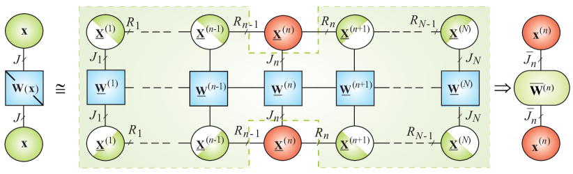
Figure 3.20: A tensor network to compute, in the TT format, the $\ell_{q}$-norm of a huge-scale vector ${\bf x}\in\mathbb{R}^{J},\;\;J=J_{1}J_{2}\cdots J_{N}$, using the IRLS (weighted $\ell_{2}$-norm).

A simple approach in this direction would be to apply Iteratively Reweighted Least Squares (IRLS) methods [Candes et al., 2008], whereby the $\ell_{1}$-norm is replaced by the reweighted $\ell_{2}$-norm (see Figure 3.20) [Lee and Cichocki, 2016a], that is

$$\|{\bf x}\|_{1}={\bf x}^{\text{T}}{\bf W}{\bf x}=\sum_{j=1}^{J}w_{j}x_{j}^{2},$$ (3.92)

where ${\bf W}({\bf x})=\mathop{\rm diag}\nolimits(w_{1},w_{2},\ldots,w_{J})$, with the diagonal elements $w_{j}=|x_{j}|^{-1}$. For a slightly more general scenario with the $\ell_{q}$-norm ($q\leq 1$), we have

$$\|{\bf x}\|_{q}^{q}={\bf x}^{\text{T}}{\bf W}({\bf x}){\bf x},$$ (3.93)

where the diagonal elements are $w_{j}=[|x_{j}|^{2}+\varepsilon^{2}]^{q/2-1}$, and $\varepsilon>0$ is a very small number needed to avoid divergence for a small $x_{j}$ [Candes et al., 2008].

Similarly, for the non-overlapping group LASSO [Chen et al., 2014]

$$\|{\bf x}\|_{q,1}^{q}=\sum_{k}\|{\bf x}_{g_{k}}\|^{q}_{q}={\bf x}^{\text{T}}{\bf W}({\bf x}){\bf x},$$ (3.94)

where ${\bf W}$ is a block diagonal matrix ${\bf W}=\mathop{\rm diag}\nolimits({\bf W}_{1},{\bf W}_{2},\ldots,{\bf W}_{K})$, with every diagonal sub-matrix ${\bf W}_{k}$, given by $[{\bf W}_{k}]_{jj}=(|x_{j}^{(g_{k})}|^{2}+\varepsilon^{2})^{q/2-1}$. In practice, it is sufficient to approximate the diagonal matrix ${\bf W}({\bf x})$ in a tensorized form by a rank one tensor, that is, with the TT rank of unity.

Figure 3.21: Illustration of computation of the enrichment tensor $\underline{{\bf Z}}^{(n)}\in\mathbb{R}^{R_{n-1}\times J_{n}\times Q_{n}}$ in the AMEn algorithm for solving systems of huge linear equations. The bottom panel shows contraction of TT networks.

In the simplest scenario, upon dividing the datasets into an appropriate number of sub-groups, the huge-scale standard LASSO problem can be converted into a set of low-dimension group LASSO sub-problems, given by (see also the first sub-networks in Figure 3.21)

$$\min_{{\bf x}^{(n)}\in\mathbb{R}^{R_{n-1}J_{n}R_{n}}}\!\biggl{(}\!{\bf x}^{(n)\;\text{T}}\overline{\bf A}^{(n)}{\bf x}^{(n)}-2[{\bf x}^{(n)}]^{\text{T}}\overline{\bf b}^{(n)}+\gamma\!\sum_{j_{n}=1}^{J_{n}}\|\underline{{\bf X}}^{(n)}(:,j_{n},:)\|_{F}\!\biggr{)}$$

which can be solved by any efficient algorithm for the group LASSO, e.g., by ADMM methods [Boyd et al., 2011].

3.9 Truncated Optimization Approach in TT Format

A wide class of optimization problems can be solved by iterative algorithms which in general can be written as

$${\bf x}_{k+1}={\bf x}_{k}+\Delta{\bf x}_{k}={\bf x}_{k}+{\bf z}_{k},$$ (3.96)

where ${\bf x}\in\mathbb{R}^{I}$ is a vector of the cost function $J({\bf x})$ and vector ${\bf z}=\Delta{\bf x}\in\mathbb{R}^{I}$ is the update vector, which can take various forms, e.g.,

1. ${\bf z}_{k}=-\eta_{k}\nabla J({\bf x}_{k})$, for gradient descent methods, where $\eta_{k}>0$ is a learning rate, and $\nabla J({\bf x}_{k})$ is the gradient vector of the cost function $J({\bf x})$ at the current iteration;

2. ${\bf z}_{k}=-\eta_{k}{\bf M}^{-1}_{k}\nabla J({\bf x}_{k})$, for preconditioned gradient descent, e.g., preconditioned conjugate gradient (CG), where ${\bf M}\in\mathbb{R}^{I\times I}$ is the preconditioned matrix;

3. ${\bf z}_{k}=-\eta_{k}{\bf H}^{-1}_{k}\nabla J({\bf x}_{k})$ for quasi-Newton methods, where ${\bf H}\in\mathbb{R}^{I\times I}$ is an approximate Hessian;

4. ${\bf z}_{k}=-\eta_{k}{\bf g}_{k}$, for subgradient methods, where ${\bf g}$ is subgradient.

To date, the following cost functions and corresponding gradients have been investigated in connection with tensor networks [Lebedeva, 2011, Ballani and Grasedyck, 2013, Dolgov, 2013]

• $\nabla J({\bf x}_{k})\propto{\bf A}^{\text{T}}{\bf A}{\bf x}_{k}-{\bf A}^{\text{T}}{\bf b}$ for the squared residual $J({\bf x})=\|{\bf A}{\bf x}-{\bf b}\|^{2}$;

• $\nabla J({\bf x}_{k})\propto{\bf A}{\bf x}_{k}-{\bf b}$ for $J({\bf x})={\bf x}^{\text{T}}{\bf A}{\bf x}-2{\bf b}^{\text{T}}{\bf x}$. In this case the process (3.96) is often referred to as a preconditioned (non-stationary) Richardson iteration;

• $\nabla J({\bf x}_{k})\propto{\bf A}{\bf x}_{k}-{\bf x}_{k}\lambda_{k}$ with $\lambda_{k}={\bf x}_{k}^{\text{T}}{\bf A}{\bf x}_{k}$, for the Rayleigh quotient $J({\bf x})={\bf x}^{\text{T}}{\bf A}{\bf x}$ with $\|{\bf x}\|^{2}=1$, which is an orthogonal projection of the gradient of $J$ onto the tangent space of a sphere, or a Stiefel manifold in general [Absil et al., 2008].

Since huge scale optimization problems are intractable, we need to represent vectors and corresponding matrices in distributed tensor formats. In a simplest scenario we can construct two TT networks, one representing vector ${\bf x}$ and the other representing approximately gradient vector ${\bf z}$, as illustrated in Figure 3.22. Assuming that both huge vectors ${\bf x}$ and ${\bf z}$ are approximately represented in TT formats, the summation of two TT networks leads to a new TT network, for which the slices of the cores are given by (cf. Part 1 [Cichocki et al., 2016])

$${\bf X}_{i_{n}}^{(n)} \leftarrow \left[\begin{matrix}{\bf X}_{i_{n}}^{(n)}&{\bf 0}\\ {\bf 0}&{\bf Z}_{i_{n}}^{(n)}\end{matrix}\right],\quad(n=2,3\ldots,N-1)$$ (3.97)

with the border cores

$${\bf X}_{i_{1}}^{(1)}\leftarrow\left[{\bf X}_{i_{1}}^{(1)},{\bf Z}_{i_{1}}^{(1)}\right],\qquad{\bf X}_{i_{N}}^{(N)} \leftarrow \left[\begin{matrix}{\bf X}_{i_{N}}^{(N)})\\ h\;{\bf Z}_{i_{N}}^{(N)}\end{matrix}\right],$$ (3.98)

while for the right to left sweep we have

$${\bf X}_{i_{1}}^{(1)}\leftarrow[\underline{{\bf X}}_{i_{1}}^{(1)},{\bf Z}_{i_{1}}^{(1)}],\;\;{\bf X}_{i_{n}}^{(n)} \leftarrow \left[\begin{matrix}{\bf X}_{i_{n}}^{(n)}&0\\ 0&{\bf Z}_{i_{n}}^{(n)}\end{matrix}\right],\;\;(n=1,2,\ldots,N-1)$$

$${\bf X}_{i_{N}}^{(N)} \leftarrow \left[\begin{matrix}{\bf X}_{i_{N}}^{(N)})\\ h\;{\bf Z}_{i_{N}}^{(N)}\end{matrix}\right].$$ (3.99)

After the enrichment of the core $\underline{{\bf X}}^{(n)}$, it needs to be orthogonalized in order to keep slice matrices orthogonal. Figure 3.22 illustrates the preconditioned gradient step (3.96), where the solution vector ${\bf x}_{k}$ and the preconditioned gradient ${\bf z}_{k}=-\alpha_{k}{\bf M}^{-1}_{k}\nabla J({\bf x}_{k})$ are represented in TT formats. Note that the TT ranks $\{S_{n}\}$ of the preconditioned gradient ${\bf z}_{k}$ are typically quite large due to the operations involved in the computation of the gradient.

Recall that the basic linear algebraic operations such as the matrix-by-vector multiplication can be performed efficiently, with a logarithmic computational complexity, via the TT representations for large matrices and vectors. Since the algebraic operations on TT formats usually result in increased TT ranks, truncation (e.g., TT-rounding [Oseledets, 2011a]) needs to be subsequently performed. It should be emphasized that truncated iteration methods are not limited to the TT format but also apply to any low-rank tensor formats.

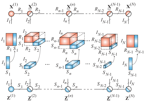
Figure 3.22: A (preconditioned) gradient step within a truncated iteration method in the TT format. The current solution vector ${\bf x}_{k}$ and the (preconditioned) gradient vector ${\bf z}_{k}=-\alpha_{k}{\bf M}^{-1}_{k}\nabla J({\bf x}_{k})$ are represented in the TT format, ${\bf x}_{k}=\text{vec}(\mathopen{\hbox{\set@color${\langle}$}\kern-1.94444pt\leavevmode\hbox{\set@color${\langle}$}}{\bf X}^{(1)},\underline{{\bf X}}^{(2)},\ldots,{\bf X}^{(N)}\mathclose{\hbox{\set@color${\rangle}$}\kern-1.94444pt\leavevmode\hbox{\set@color${\rangle}$}})$ and ${\bf z}_{k}=\text{vec}(\mathopen{\hbox{\set@color${\langle}$}\kern-1.94444pt\leavevmode\hbox{\set@color${\langle}$}}{\bf Z}^{(1)},\underline{{\bf Z}}^{(2)},\ldots,{\bf Z}^{(N)}\mathclose{\hbox{\set@color${\rangle}$}\kern-1.94444pt\leavevmode\hbox{\set@color${\rangle}$}})$. The addition of these two vectors can be performed by a partial (mode-2) direct sum between core tensors as $\underline{{\bf X}}^{(n)}\oplus_{2}\underline{{\bf Z}}^{(n)}\in\mathbb{R}^{(R_{n-1}+S_{n-1})\times I_{n}\times(R_{n}+S_{n})}$.

Let ${\bf T}_{\epsilon}$ denote a truncation operator which truncates ranks of a tensor format with a tolerance $\epsilon>0$. Truncated iteration methods can be described as a preconditioned gradient step combined with truncation, as

$${\bf x}_{k+1}={\bf T}_{\epsilon}\left({\bf x}_{k}-\alpha_{k}{\bf T}_{\eta}({\bf M}^{-1}_{k}\nabla J({\bf x}_{k}))\right),\quad\epsilon,\eta>0.$$

The rank truncation can be carried out by a hard thresholding scheme or a soft thresholding scheme [Bachmayr et al., 2016]. In the iterative hard thresholding scheme, singular values below some threshold are set to zero as in the truncated SVD or TT rounding [Oseledets, 2011a]. In the iterative soft thresholding scheme, on the other hand, each of the singular values is shrunk to zero by the function $s_{\kappa}(x)=\text{sign}(x)\max(|x|-\kappa,0)$ for some $\kappa\geq 0$. The soft thresholding is equivalent to minimizing the nuclear norm of a matrix, which is a convex relaxation of rank. Both types of thresholding schemes adaptively change the ranks during iteration process.

The truncated iteration approach has been already investigated and extensively tested for several very large-scale data applications using various low-rank tensor formats, especially for:

• Solving huge systems of linear equations and discretization of PDEs by iterative algorithms (e.g., Richardson, CG GMRES) and combined with CP format [Beylkin and Mohlenkamp, 2005, Khoromskij and Schwab, 2011], CP and Tucker formats [Billaud-Friess et al., 2014], TT format [Khoromskij and Oseledets, 2010, Dolgov, 2013], HT format [Kressner and Tobler, 2011a, Bachmayr and Dahmen, 2015, Bachmayr and Schneider, 2016], and a subspace projection method combined with HT format [Ballani and Grasedyck, 2013];

• A subspace projection method combined with HT format [Ballani and Grasedyck, 2013];

• Computing extreme eigenvalues and corresponding eigenvectors by Lanczos method combined with TT format [Huckle and Waldherr, 2012, Huang et al., 2016], preconditioned inverse iteration with TT format [Mach, 2013], block CG method (LOBPCG) combined with TT format [Lebedeva, 2011] and with HT format [Kressner and Tobler, 2011b];

• Iterative hard thresholding for low-rank matrix/tensor completion [Foucart and Rauhut, 2013, Tanner and Wei, 2013].

An advantage of truncated iteration methods is that we do not need to construct tensor networks for a specific cost (loss) function. Moreover, theoretical global convergence properties hold under some restricted conditions (see [Bachmayr et al., 2016] for more detail). In addition, due to the analogy between low-rank truncation and sparse signal estimation techniques, truncated iteration-type algorithms are also suitable for large-scale compressed sensing [Blumensath and Davies, 2009].

However, truncated iteration methods have a few drawbacks. They require the estimation of several auxiliary vectors. In addition to the desired vector, ${\bf x}$, right-hand vector, ${\bf z}$, need to have a low-rank representation in the specific tensor format. For example, in the GMRES method [Dolgov, 2013], even if the solution vector and the right-hand side vector are well approximated by the TT format, the residuals and Krylov vectors involved in intermediate iterations usually have high TT ranks. Moreover, all the core tensors and factor matrices of the solution vector have to be truncated at each iteration step, which often incurs high computational costs, especially when ranks are large.

3.10 Riemannian Optimization for Low-Rank Tensor Manifolds

Methods of Riemannian Optimization (RO) have been recently a subject of great interest in data analytics communities; see, for example, [Absil et al., 2008, 2007, Bonnabel, 2013, Cambier and Absil, 2016, Bento et al., 2016]. Some optimization problems discussed in previous sections, can be naturally formulated on Riemannian manifolds, so as to directly benefit from the underlying geometric structures that can be exploited to significantly reduce the cost of obtaining solutions. Moreover, from a Riemannian geometry point of view, constrained optimization problems can often be viewed as unconstrained ones. It is therefore natural to ask whether Riemannian optimization can also help open up new research directions in conjunction with tensor networks; see for example [Ishteva et al., 2011, Kasai and Mishra, 2015, Steinlechner, 2016a, Zhou et al., 2016, Sato et al., 2017].

Riemannian optimization for tensors can be formulated in the following generalized form

$$\min_{\underline{\mathbf{{X}}}\in\mathcal{M}_{r}}\ J(\underline{\mathbf{{X}}}),$$ (3.100)

where $J(\underline{{\bf X}})$ is a scalar cost function of tensor variables and the search space, $\mathcal{M}_{r}$, is smooth, in the sense of a differentiable manifold structure. Note that to perform optimization, the cost function needs to be defined for points on the manifold $\mathcal{M}_{r}$. The optimization problem in the form (3.100) is quite general, and most of the basic optimization problems can be cast into this form.

In our applications of RO, $\mathcal{M}_{r}$ is a certain low-rank tensor manifold. One of the potential advantages of using Riemannian optimization tools for tensors is therefore that the intrinsic geometric and algebraic properties of the manifold allow us to convert a constrained optimization problems to an unconstrained one, in other words, to perform unconstrained optimization on a constrained space.

Manifold structure for Tucker model. The Riemannian optimization (also called the differential geometric optimization) has been successfully applied to the computation of the best Tucker approximation [Ishteva et al., 2009, 2011, Steinlechner, 2016a], whereby the Tucker manifold structure can be formulated through a set of Tucker tensors of fixed multilinear rank $r_{ML}=\{R_{1},\ldots,R_{N}\}$

$$\mathcal{M}_{r}:=\{\underline{{\bf X}}\in\mathbb{R}^{I_{1}\times\cdots\times I_{N}}\;|\;\mbox{rank}_{ML}(\underline{{\bf X}})=r_{ML}\},$$

which forms a smooth embedded submanifold of $\mathbb{R}^{I_{1}\times\cdots\times I_{N}}$ of dimension

$$\dim\mathcal{M}_{r}=\prod_{n=1}^{N}R_{n}+\sum_{n=1}^{N}(R_{n}I_{n}-R^{2}_{n}).$$ (3.101)

Manifold structure for TT model. The set of TT tensors of fixed TT-rank, $r_{TT}=\{R_{1},\ldots,R_{N-1}\}$, given by

$$\mathcal{M}_{r}:=\{\underline{{\bf X}}\in\mathbb{R}^{I_{1}\times\cdots\times I_{N}}\;|\;\mbox{rank}(\underline{{\bf X}})_{TT}=r_{TT}],$$

forms a smooth embedded submanifold of $\mathbb{R}^{I_{1}\times\cdots\times I_{N}}$ of dimension

$$\dim\mathcal{M}_{r}=\sum_{n=1}^{N}R_{n-1}I_{n}R_{n}-\sum_{n=1}^{N-1}R^{2}_{n},$$ (3.102)

with $R_{N}=1$. If the inner product of two tensors induces a Euclidean metric on the embedding space $\mathbb{R}^{I_{1}\times\cdots\times I_{N}}$, then the above submanifold $\mathcal{M}_{r}$ is a Riemannian manifold [Holtz et al., 2012b, Steinlechner, 2016a, Uschmajew and Vandereycken, 2013].

Similar results are also available for the more general hierarchical Tucker models. For example, [Uschmajew and Vandereycken, 2013] developed the manifold structure for the HT tensors, while Lubich et al. [2013] developed the concept of dynamical low-rank approximation for both HT and TT formats. Moreover, Riemannian optimization in the Tucker and TT/HT formats has been successfully applied to large-scale tensor completion problems [Da Silva and Herrmann, 2013, Kasai and Mishra, 2015, Zhou et al., 2016].

It is important to emphasize that the condition of full TN rank is a pre-requisite for the sets $\mathcal{M}_{r}$ to be smooth manifolds. Otherwise, a set of tensors for which the ranks are only bounded from above by $R_{\max}$ would no longer be a smooth manifold, but an algebraic variety, for which special optimization methods are needed, at least for theoretical justification.

The fundamental and basic algorithms for Riemannian optimization [Absil et al., 2008] are quite attractive, but are still not widely used as they are more technically complicated than, e.g., standard gradient descent or conjugate gradient (CG) used in the classical optimization algorithms of low-rank tensor manifolds. However, in many cases Riemannian manifolds can be relatively easily implemented and often provide much better performance than the standard algorithms [Kressner et al., 2014b, Kasai and Mishra, 2015].

The MANOPT package [Boumal et al., 2014] (for a Python version see [Koep and Weichwald, 2016]) provides a useful interface for many standard matrix Riemannian optimization techniques, however, extensions for tensors (especially in high dimensions) are not easy and should be performed very carefully. The key idea is to work in the full space, but with the restrictions: i) the solution lies on a non-linear smooth manifold, and ii) the manifold condition is enforced implicitly (i.e., the derivatives with respect to the parametrization are not explicitly used).

In order to apply optimization algorithms based on line search, we must consider a direction on a manifold. The tangent space at $\underline{{\bf X}}\in\mathcal{M}_{r}$ is the set of all tangent vectors (directions) at $\underline{{\bf X}}$, denoted by $T_{\underline{{\bf X}}}\mathcal{M}_{r}$. The tangent space is a linear space, which, at a point on the manifold, provides us with a vector space of tangent vectors that allow us to find a search direction on the manifold. A Riemannian metric allows us to compute the angle and length of directions (tangent vectors). Roughly speaking, the optimization is performed on the tangent space, by either performing linear search or building a local model, in order to estimate the tangent vector and perform the next iteration on the manifold. The retraction operator provides a method to map the tangent vector to the next iterate (see the next section).

The smoothness condition of the manifold is crucial, since this allows us to define a tangent space, $T_{\underline{\mathbf{{X}}}}\mathcal{M}_{r}$, for each point on the manifold, which locally approximates the manifold with second-order accuracy. Such a linearization of the manifold allows us to compute the next approximation restricted to the tangent space, which is a linear subspace. We shall next describe the general setting in which Riemannian optimization resides.

3.10.1 Simplest Riemannian Optimization Method: Riemannian Gradient Descent

Consider a smooth manifold, $\mathcal{M}_{r}$, in a vector space of tensors. The simplest optimization method is gradient descent which has the form

$$\underline{\mathbf{{X}}}_{k+1}=\underline{\mathbf{{X}}}_{k}-\alpha_{k}\nabla J(\underline{\mathbf{{X}}}_{k}),$$

where $\alpha_{k}>0$ is the step size. For a sufficiently small $\alpha$, the value of the cost function $J(\underline{\mathbf{{X}}})$ will decrease. However, this does not provide a restriction that $\underline{\mathbf{{X}}}_{k+1}$ should lie on a manifold; although $\underline{\mathbf{{X}}}_{k}$ is on the manifold, the step in the direction of the negative gradient will leave the manifold. If the manifold is a linear subspace, then the solution is quite simple — we just need to take a projected gradient step, i.e., project $\nabla J(\underline{\mathbf{{X}}}_{k})$ to this subspace. For a general smooth manifold we can do the same, but the projection is computed onto the tangent space of the manifold at the current iteration point, that is

$$\underline{\mathbf{{X}}}_{k+1}=\underline{\mathbf{{X}}}_{k}-\alpha_{k}P_{T_{\underline{\mathbf{{X}}}_{k}}\mathcal{M}_{r}}(\nabla J(\underline{\mathbf{{X}}}_{k})).$$ (3.103)

The continuous version of (3.103) will have the following projected gradient flow

$$\frac{d\underline{\mathbf{{X}}}}{dt}=-P_{T_{\underline{\mathbf{{X}}}}\mathcal{M}_{r}}(\nabla J(\underline{\mathbf{{X}}})),$$ (3.104)

and it is quite easy to see that if $\underline{\mathbf{{X}}}(0)$ (initial conditions) is on the manifold, then the whole trajectory $\underline{\mathbf{{X}}}(t)$ will be on the manifold. This is, however, not guaranteed for the discretized version in (3.103), which can be viewed as a forward Euler scheme applied to (3.104). This also has important computational consequences.

An iterative optimization algorithm involves the computation of a search direction and then performing a step in that direction. Note that all iterations on a manifold $\mathcal{M}_{r}$ should be performed by following geodesics. However, in general geodesics may be either expensive to compute or even not available in a closed form. To this end, in practice, we relax the constraint of moving along geodesics by applying the concept of Retraction, which is any map $R_{{\bf X}}:T_{\underline{{\bf X}}}\mathcal{M}_{r}\rightarrow\mathcal{M}_{r}$ that locally approximates a geodesic, up to first order, thereby reducing the computational cost of the update and ensuring convergence of iterative algorithms.

Figure 3.23: The concept of retraction for a smooth submanifold. The iteration process for Riemannian gradient descent for optimization on a smooth submanifold $\mathcal{M}_{r}$ embedded in a Euclidean space consists of three-steps: 1) an update in the Euclidean space (which is not computed explicitly), 2) a linear projection of the gradient to the tangent space $T_{\underline{\mathbf{{X}}}}\mathcal{M}_{r}$, and 3) a retraction to the manifold $\mathcal{M}_{r}$. See also Equation (3.105) and [Kressner et al., 2016].

More precisely the Retraction can be defined, as follows

Definition 1

[Adler et al., 2002] A mapping $R_{{\bf X}}$ is called the retraction, if

1. $R_{{\bf X}}(\underline{\mathbf{{X}}},\underline{\mathbf{{Z}}})\in\mathcal{M}_{r}$ for $\underline{\mathbf{{Z}}}\in T_{\underline{\mathbf{{X}}}}\mathcal{M}_{r}$,

2. $R_{{\bf X}}$ is defined and smooth in a neighborhood of the zero section in $T_{\underline{\mathbf{{X}}}}\mathcal{M}_{r}$,

3. $R_{{\bf X}}(\underline{\mathbf{{X}}},\underline{\mathbf{{0}}})=\underline{\mathbf{{X}}}$ for all $\underline{\mathbf{{X}}}\in\mathcal{M}_{r}$,

4. $\frac{d}{dt}R_{{\bf X}}(\underline{\mathbf{{X}}},t\underline{\mathbf{{Z}}})\mid_{t=0}=\underline{\mathbf{{Z}}},\quad\mbox{for all }\underline{\mathbf{{X}}}\in\mathcal{M}_{r}\quad\mbox{and }\;\;\underline{\mathbf{{Z}}}\in T_{\underline{\mathbf{{X}}}}\mathcal{M}_{r}$.

For low-rank matrices and tensors with fixed TT-ranks, the simplest retraction is provided by respective SVD and TT-SVD algorithms, however, there are many other types of retractions; for more detail we refer to the survey [Absil and Oseledets, 2015].

Finally, the Riemannian gradient descent method has the form

$$\underline{\mathbf{{X}}}_{k+1}=R_{{\bf X}}(\underline{\mathbf{{X}}}_{k},\;-\alpha_{k}P_{T_{\underline{\mathbf{{X}}}_{k}}\mathcal{M}_{r}}(\nabla J(\underline{\mathbf{{X}}}_{k}))).$$ (3.105)

Figure 3.23 illustrates the three-step procedure within the Riemannian gradient descent iteration given in (3.105). From the implementation viewpoint, the main difficulty is to compute the projection of the gradient $P_{T_{\underline{\mathbf{{X}}}_{k}}\mathcal{M}_{r}}(\nabla J(\underline{\mathbf{{X}}}_{k}))$. For the optimization problems mentioned above, this projection can be computed without forming the full gradient.

3.10.2 Advanced Riemannian Optimization Methods

Vector transport. More advanced optimization techniques, such as conjugate-gradient (CG)-type methods and quasi-Newton methods, use directions from previous iteration steps. However, these directions lie in different tangent spaces which are different from the corresponding optimization in Euclidean spaces. To this end, we need to employ the concept of vector transport, which plays a crucial role in Riemannian optimization. The idea of vector transport is quite simple: it represents a mapping from one tangent space $T_{\underline{\mathbf{{X}}}}\mathcal{M}_{r}$, to another tangent space, $T_{\underline{\mathbf{{Y}}}}\mathcal{M}_{r}$. For low-rank matrix/tensor manifolds, the orthogonal projection to a tangent space $P_{T_{\underline{\mathbf{{Y}}}}\mathcal{M}_{r}}$ is an example of a vector transport.

Figure 3.24: Concept of the vector transport for the Riemannian CG method for the optimization on a manifold $\mathcal{M}_{r}$. The update direction, $\eta$, at the previous iteration, which belongs to the tangent space $T_{\underline{{\bf X}}}\mathcal{M}_{r}$, is mapped to a tangent vector in the tangent space $T_{\underline{{\bf Y}}}\mathcal{M}_{r}$, via a suitably defined mapping (i.e., the vector transport) denoted by $T_{\underline{{\bf X}}\rightarrow\underline{{\bf Y}}}$. See also Algorithm (13).

Riemannian CG Method. Figure 3.24 illustrates the vector transport during a Riemannian CG iteration, which transforms a tangent vector in $T_{\underline{{\bf X}}}\mathcal{M}_{r}$ at a certain point $\underline{{\bf X}}\in\mathcal{M}_{r}$ to another tangent space $T_{\underline{{\bf Y}}}\mathcal{M}_{r}$ at $\underline{{\bf Y}}\in\mathcal{M}_{r}$. In the Riemannian CG iteration, the previous update direction $\mbox{\boldmath$\eta$}_{k-1}\in T_{\underline{{\bf X}}_{k-1}}\mathcal{M}_{r}$ is mapped to a tangent vector in $T_{\underline{{\bf X}}_{k}}\mathcal{M}_{r}$, and the transformed vector is combined with the Riemannian (projected) gradient vector to complete the CG iteration. Now, by using the projection onto the tangent space, retraction, and vector transport, we can immediately implement a general nonlinear CG method (Riemannian CG method) (see Algorithm 13).

1:  Initial guess $\underline{\mathbf{{X}}}_{0}\in\mathcal{M}_{r}$ 2:  $\mbox{\boldmath$\eta$}_{0}:=-P_{T_{\underline{\mathbf{{X}}}_{0}}\mathcal{M}_{r}}(\nabla J(\underline{\mathbf{{X}}}_{0}))$ $\alpha_{0}=\arg\min_{\alpha}J(\underline{\mathbf{{X}}}_{0}+\alpha\mbox{\boldmath$\eta$}_{0})$ 3:  $\underline{\mathbf{{X}}}_{1}=R_{{\bf X}}(\underline{\mathbf{{X}}}_{0},\alpha_{0}\mbox{\boldmath$\eta$}_{0}).$ 4:  for $k=1,\ldots$ do 5:     $\mbox{\boldmath$\xi$}_{k}:=P_{T_{\underline{\mathbf{{X}}}_{k}}\mathcal{M}_{r}}(\nabla J(\underline{\mathbf{{X}}}_{k}))$ 6:     $\mbox{\boldmath$\eta$}_{k}:=-\mbox{\boldmath$\xi$}_{k}+\beta_{k}T_{\underline{\mathbf{{X}}}_{k-1}\rightarrow\underline{\mathbf{{X}}}_{k}}\mbox{\boldmath$\eta$}_{k-1}$ 7:     $\alpha_{k}=\arg\min_{\alpha}J(\underline{\mathbf{{X}}}_{k}+\alpha\mbox{\boldmath$\eta$}_{k})$ 8:     Find the smallest integer $m\geq 0$ such that $J(\underline{\mathbf{{X}}}_{k})-J(R_{{\bf X}}(\underline{\mathbf{{X}}}_{k},2^{-m}\alpha_{k}\mbox{\boldmath$\eta$}_{k}))\geq\delta\;\langle\mbox{\boldmath$\eta$}_{k},2^{-m}\alpha_{k}\mbox{\boldmath$\eta$}_{k}\rangle$ 9:     $\underline{\mathbf{{X}}}_{k+1}:=R_{{\bf X}}(\underline{\mathbf{{X}}}_{k},2^{-m}\alpha_{k}\mbox{\boldmath$\eta$}_{k}).$ 10:  end for

Algorithm 13 Riemannian CG method

The main problem in Riemannian CG methods is the computation of the parameter $\beta_{k}$ within the conjugate gradient direction. To this end, as suggested in Kressner et al. [2016] the Polak-Ribiere update formula [Nocedal and Wright, 2006] can be adapted to Riemannian optimization [Absil et al., 2008].

3.10.3 Riemannian Newton Method

The implementation of Riemannian Newton-type algorithms is much more complicated, but follows the standard concept of Newton optimization methods. The local search direction, $\mbox{\boldmath$\xi$}_{k}$, is determined from the correction equation [Absil et al., 2008] as

$${\bf H}_{\underline{\mathbf{{X}}}_{k}}\mbox{\boldmath$\xi$}_{k}=-P_{T_{\underline{\mathbf{X}}_{k}}\mathcal{M}_{r}}\nabla J(\underline{\mathbf{{X}}}_{k}),$$ (3.106)

where the Riemannian Hessian, ${\bf H}_{\underline{\mathbf{{X}}}_{k}}:T_{\underline{\mathbf{{X}}}_{k}}\mathcal{M}_{r}\rightarrow T_{\underline{\mathbf{{X}}}_{k}}\mathcal{M}_{r}$, is defined as [Absil et al., 2013, Kressner et al., 2016]

$${\bf H}_{\underline{\mathbf{{X}}}_{k}}=P_{T_{\underline{\mathbf{X}}_{k}}\mathcal{M}_{r}}\left(\nabla^{2}J(\underline{\mathbf{{X}}}_{k})+P^{\prime}_{\underline{\mathbf{{X}}}_{k}}\nabla J(\underline{\mathbf{{X}}}_{k})\right)P_{T_{\underline{\mathbf{X}}_{k}}\mathcal{M}_{r}},$$ (3.107)

and $P^{\prime}_{\underline{\mathbf{{X}}}_{k}}$ is the derivative of the projector $P_{T_{\underline{\mathbf{X}}}\mathcal{M}_{r}}$ with respect to $\underline{\mathbf{{X}}}$. The second term in the sum corresponds to the curvature of the manifold. If the true minimizer is on the manifold, then $\nabla J(\underline{\mathbf{{X}}}_{*})=\underline{\mathbf{{0}}}$, and at least in the vicinity of the solution the second term plays no role. However, this term can cause problems with stability if the solution is close to a singular point, where the tangent space can exhibit considerable variation. In many cases, only the first term in (3.107) is used, leading to the approximate Newton method, also known as the Gauss-Newton method in constrained optimization, given by

$$\widehat{{\bf H}}_{\underline{\mathbf{{X}}}_{k}}=P_{T_{\underline{\mathbf{X}}_{k}}\mathcal{M}_{r}}\,\nabla^{2}J\,P_{T_{\underline{\mathbf{X}}_{k}}\mathcal{M}_{r}}.$$ (3.108)

If $\nabla^{2}J$ is positive definite (e.g., for strongly convex $J(\underline{{\bf X}})$) the matrix $\widehat{{\bf H}}_{\underline{\mathbf{{X}}}}$ is also nonnegative definite.

The Gauss-Newton method has a simple interpretation: we approximate the manifold by a tangent space, and seek for the minimum of a specific cost function $J(\underline{{\bf X}})$ on the tangent space. However, the theoretical justification of such methods, even for relatively simple low-rank matrix cases, is still an open problem. Recently, in order to achieve a better global convergence, an alternative version of the Riemannian Newton method called the Trust-Region scheme was developed by Absil et al. [2007], Ishteva et al. [2011], Boumal and Absil [2011].

Retraction and vector transport are critical operations to the success of sophisticated Riemannian optimization algorithms, such as Riemannian CG, Newton and/or quasi-Newton methods. Retraction is used to obtain the next iterate and vector transport is used to compare tangent vectors in different tangent spaces and to transport operators from one tangent space to another tangent space.

Parametrization. When considering the tensor case, the whole concept above applies to the matrix-based tensor formats, such as the Tucker format and TT format. However, the concept does not apply to the CP decomposition, since the set of all tensors with a given canonical rank does not form a manifold (CP decomposition is unique).

3.10.4 Low-Rank TT-Manifold

Consider a set of $N$th-order tensors in TT formats, with all TT-ranks equal to $(R_{1},\ldots,R_{N-1})$. This set can also be thought of as an intersection of $(N-1)$ low-rank matrix manifolds, since the $n$th TT-rank of a tensor $\underline{{\bf X}}$ is equal to the matrix rank of its $n$th mode unfolding ${\bf X}_{<n>}$.

A tensor in the TT-format can be parameterized in the form

$$\underline{{\bf X}}(i_{1},\ldots,i_{N})={\bf X}^{(1)}_{i_{1}}\cdots{\bf X}^{(N)}_{i_{N}},$$

where ${\bf X}^{(n)}_{i_{n}}\in\mathbb{R}^{R_{n-1}\times R_{n}}$ are slices of TT-cores $\underline{\mathbf{X}}^{(n)}$ .

Tangent space of TT. The tangent space at a point $\underline{{\bf X}}$ in the TT-manifold is defined as a set of tensors of the form

$$\delta\underline{{\bf X}}(i_{1},\ldots,i_{N})=\delta{\bf X}^{(1)}_{i_{1}}{\bf X}^{(2)}_{i_{2}}\cdots{\bf X}^{(N)}_{i_{N}}+\cdots+{\bf X}^{(1)}_{i_{1}}{\bf X}^{(2)}_{i_{2}}\cdots\delta{\bf X}^{(N)}_{i_{N}},$$ (3.109)

and is parameterized by the variations of the TT-cores $\delta\underline{{\bf X}}^{(n)}$.

We denote the QR decompositions of unfoldings ${\bf X}^{\leq n}$ and ${\bf X}^{\geq n+1}$ as

$${\bf X}^{\leq n}={\bf Q}_{\leq n}{\bf R}_{\leq n},\quad({\bf X}^{\geq n+1})^{\text{T}}={\bf Q}_{\geq n+1}{\bf R}_{\geq n+1},$$

and the orthogonal projectors onto the column spaces of these matrices can be introduced in the form

$${\bf P}_{\leq n}={\bf Q}_{\leq n}{\bf Q}^{\text{T}}_{\leq n},\quad{\bf P}_{\geq n}={\bf Q}_{\geq n}{\bf Q}^{\text{T}}_{\geq n}.$$

Using these projectors the orthogonal projector onto the tangent space, $P_{T_{\underline{\mathbf{X}}}\mathcal{M}_{r}}(\underline{\mathbf{Z}})$, can be written as [Holtz et al., 2012b, Lubich et al., 2015]

$$P_{T_{\underline{\mathbf{X}}}\mathcal{M}_{r}}(\underline{\mathbf{Z}})=\sum_{n=1}^{N}P_{\underline{\mathbf{X}}}^{\leq n}(P_{\underline{\mathbf{X}}}^{\geq n+1}(\underline{\mathbf{Z}}))\,,$$ (3.110)

where

$$P_{\underline{\mathbf{X}}}^{\leq n}(\underline{\mathbf{Z}}) = \operatorname{Ten}({\bf P}_{\leq n}{\bf Z}_{<n>})\,,$$ (3.111)

$$P_{\underline{\mathbf{X}}}^{\geq n+1}(\underline{\mathbf{Z}}) = \operatorname{Ten}({\bf Z}_{<n>}{\bf P}_{\geq n+1}),$$ (3.112)

and $\operatorname{Ten}({\bf Z})$ is an inverse operator of the matricization of the tensor $\underline{\mathbf{X}}$, i.e., creating a tensor of the same size as the tensor $\underline{\mathbf{X}}$.

It should be noted that any point on a tangent space has TT-ranks bounded by $(2R_{1},\ldots,2R_{N-1})$, thus the computation of the TT-rank $(R_{1},\ldots,R_{N-1})$ approximation is possible by running the rounding procedure (or the TT-SVD) at the $\mathcal{O}(NIR^{3})$ cost, where we assumed that $I_{n}=I,\quad R_{n}=R.$ Therefore, many Riemannian optimization algorithms for low rank matrices remain formally the same, making the Riemannian optimization a promising and powerful tool for optimization over TT-manifolds.

3.10.5 Dynamical Low-Rank Matrix/Tensor Approximation

Riemannian optimization is intricately connected with the concept of dynamical low-rank approximation, and although it was introduced in mathematics by Koch and Lubich [2007], its roots are in quantum mechanics and can be traced back to the so-called Dirac-Frenkel principle. Indeed, some fundamental results can be found in the quantum molecular dynamics community which has used the so-called Multi Configurational Time-Dependent Hartree (MCTDH) method already since the 1990s [Manthe et al., 1992]. As an example, consider a time-varying matrix ${\bf A}(t)$ which we wish to approximate by a low-rank matrix ${\bf X}(t)$. Of course, this can be achieved on a sample-by-sample basis, by computing SVD for each $t$, but this does not involve any “memory” about the previous steps.

A Dirac-Frenkel principle states that the optimal trajectory should not minimize the distance

$$\|{\bf A}(t)-{\bf Y}(t)\|$$

over all matrices of rank $R$, but instead the local dynamics given by

$$\|\frac{d{\bf A}}{dt}-\frac{d{\bf Y}}{dt}\|.$$ (3.113)

For the Euclidean norm, the minimization of the cost function (3.113) leads the following differential equations on manifold $\mathcal{M}_{r}$

$$\frac{d{\bf Y}}{dt}=P_{T_{\bf Y}\mathcal{M}_{r}}\frac{d{\bf A}}{dt},\quad{\bf Y}(0)\in\mathcal{M}_{r}.$$ (3.114)

In other words, the approximated trajectory ${\bf Y}(t)$ is such that the velocity $\frac{d{\bf Y}}{dt}$ always lies in the tangent space, and thus the trajectory always stays on the manifold. The dynamical approximation in (3.114) allows us to construct (and actually strictly define) low-rank approximation to the dynamical systems. If ${\bf A}(t)$ admits the representation

$$\frac{d{\bf A}}{dt}=F({\bf A},t),$$ (3.115)

which is a typical case in quantum mechanics, where the idea was first proposed, we obtain a dynamical system for the point on a low-rank manifold in the form

$$\frac{d{\bf Y}}{dt}=P_{T_{\bf Y}\mathcal{M}_{r}}F({\bf Y},t).$$ (3.116)

Such a system can be efficiently treated using only the parametrization of a point on a such manifold, thereby greatly reducing the cost (and if the manifold approximates the solution well,with a sufficiently good accuracy). Note that the continuous variant of the Riemannian gradient in (3.103) can be written exactly in the form (3.116), with

$$F({\bf Y},t)=-\nabla J.$$

Retraction is needed only in the discrete case, since in the continuous case the exact solution lies exactly on the manifold. Thus, if we have an efficient way to solve (3.116) numerically, that would give an efficient way of solving Riemannian optimization problems.

There are two straightforward ways of solving (3.116). The original approach of Koch and Lubich [2007] (later generalized to the Tucker and TT models [Koch and Lubich, 2010]) is to write down ordinary differential equations for the parameters ${\bf U}(t),{\bf S}(t),{\bf V}(t)$ of the SVD like decomposition in the form

$${\bf Y}(t)={\bf U}(t){\bf S}(t){\bf V}^{\text{T}}(t).$$

The second approach is also straightforward: apply any time integration scheme to the equation (3.116). In this case, a standard method will yield the solution which is not on the manifold, and a retraction would be needed. In Lubich and Oseledets [2014] a simple and efficient solution to this problem, referred to as the projector-splitting scheme, was proposed, based on the special structure of the manifold. This stable and explicit second-order scheme for the integration of (3.116) examines the projector onto the tangent space

$$P_{T_{\bf Y}\mathcal{M}_{r}}{\bf Z}={\bf U}{\bf U}^{\text{T}}{\bf Z}+{\bf Z}{\bf V}{\bf V}^{\text{T}}-{\bf U}{\bf U}^{\text{T}}{\bf Z}{\bf V}{\bf V}^{\text{T}}={\bf P}_{U}+{\bf P}_{V}-{\bf P}_{UV},$$

and represents it as a sum of three projectors, in order to apply the classical Strang-Marchuk splitting scheme. For each projector, the equations of dynamical low-rank approximations can now be easily integrated. Indeed, the equation

$$\frac{d{\bf Y}}{dt}=\frac{d{\bf A}}{dt}{\bf V}{\bf V}^{\text{T}},$$

has a simple solution; the ${\bf V}$ component does not change and the new point is just

$${\bf Y}_{1}={\bf Y}_{0}+({\bf A}_{1}-{\bf A}_{0}){\bf V},$$ (3.117)

where ${\bf A}_{1}={\bf A}(t+h),\quad{\bf A}_{0}={\bf A}(t).$ Similar formulas are valid for ${\bf P}_{V}$ and ${\bf P}_{UV}$. What is not trivial is the order in which the splitting steps are taken: we should make a step in ${\bf P}_{U}$, then in ${\bf P}_{UV}$, and then in ${\bf P}_{V}$. This leads to a much better convergence, and moreover an exactness result [Lubich and Oseledets, 2014] can be proven if ${\bf A}_{1}$ and ${\bf A}_{0}$ are on the manifold, and ${\bf Y}_{0}={\bf A}_{0}$, then this scheme is exact.

Through the link with the Riemannian optimization, the projector-splitting scheme can be also used here, which can be viewed as a second-order retraction [Absil and Oseledets, 2015]. A simple form can be obtained for a given ${\bf X}$ and a step ${\bf Z}$, where for the matrix case the retraction is

$${\bf U}_{1}{\bf S}_{\frac{1}{2}}=\operatorname{QR}(({\bf X}+{\bf Z}){\bf V}_{0}),\quad{\bf V}_{1}{\bf S}^{\text{T}}_{1}=\mathrm{QR}(({\bf X}+{\bf Z})^{\text{T}}{\bf U}_{1}).$$

This is just one step of a block power method, applied to $({\bf X}+{\bf Z})$. Although this is only a crude approximation of the SVD of $({\bf X}+{\bf Z})$ which is the standard retraction, the projector-splitting retraction is also a second-order retraction.

The generalization to the TT network was proposed by Lubich et al. [2015], and can be implemented within the framework of sweeping algorithms, allowing for the efficient TT-approximation of dynamical systems and solution of optimization problems with non-quadratic functionals.

3.10.6 Convergence of Riemannian Optimization Algorithms

Convergence theory for the optimization over non-convex manifolds is much more complicated than the corresponding theory in Euclidean spaces, and far from complete. Local convergence results follow from the general theory [Absil et al., 2008], however the important problem of the curvature and singular points is not yet fully addressed. One way forward is to look for the desingularization [Khrulkov and Oseledets, 2016], another technique is to employ the concept of tangent bundle. Even if the final point is on the manifold, it is not clear whether it is better to take a trajectory on the manifold. An attempt to study the global convergence was presented in [Kolesnikov and Oseledets, 2016], and even in this case, convergence to the spurious local minima is possible in a carefully designed example. Also, convergence should be considered together with low-rank approximation to the solution itself. When we are far from having converged, a rank-one approximation to the solution will be satisfactory, then the rank should gradually increase. This was observed experimentally in [Kolesnikov and Oseledets, 2016] in the form of a “staircase” convergence. So, both the local convergence, in the case when the solution is only approximately of low-rank, and the global convergence of Riemannian optimization have to be studied, but numerous applications to machine learning problems (like matrix/tensor completion) confirm its efficiency, while the applications to tensor network optimization have just started to appear.

3.10.7 Exponential Machines for Learning Multiple Interactions

Riemannian optimization methods have been recently demonstrated as a powerful approach for solving a wide variety of standard machine learning problems. In this section, we will briefly describe one such promising application [Novikov et al., 2016]. Consider machine learning tasks with categorical data, where for improved performances it is important to properly model complex interactions between the multiple features. Consider the training data, $\{({\bf x}_{m},y_{m})\}_{m=1}^{M}$, where ${\bf x}_{m}=[x_{1,m},\ldots,x_{N,m}]^{\text{T}}$ is an $N$-dimensional feature vector and $y_{m}$ the target value of the $m$-th object.

In the special case of $N=3$, the linear model which incorporates interactions between the features $x_{1},x_{2}$ and $x_{3}$, can be described by

$$\begin{split}\widehat{y}({\bf x})&=w_{000}+w_{100}x_{1}+w_{010}x_{2}+w_{001}x_{3}\\ &+w_{110}x_{1}x_{2}+w_{101}x_{1}x_{3}+w_{011}x_{2}x_{3}+w_{111}x_{1}x_{2}x_{3},\end{split}$$

where the parameters $w_{ijk}$ denote the strength of interactions between the features $x_{i},x_{j}$ and $x_{k}$ (see also Chapter 1).

Note that in the general case of $N$ features, the number of pair-wise interactions is $\mathcal{O}(N^{2})$, and the number of all possible interactions grows exponentially as $\mathcal{O}(2^{N})$. Such interactions occur, for example, in language/text analysis or in sentiment analysis where each individual word can interact with other words. To deal with the exponentially large number of parameters, Novikov et al. [2016], Stoudenmire and Schwab [2016] proposed the so-called Exponential Machines (ExM), where a large tensor of parameters is represented compactly in the TT format in order to provide low-rank regularization of the model and a reduction of the problem to a manageable scale. The so obtained linear model can be described in a general tensor form as

$$\widehat{y}(\underline{{\bf X}})=\langle\underline{{\bf W}},\underline{{\bf X}}\rangle=\sum_{i_{1}=0}^{1}\cdots\sum_{i_{N}=0}^{1}w_{i_{1},\ldots,i_{N}}\prod_{n=1}^{N}x_{n}^{i_{n}},$$

where $\underline{{\bf W}}\in\mathbb{R}^{I_{1}\times\cdots\times I_{N}}$ $(I_{n}=2\;,\forall n)$ is the tensor of parameters and $\underline{\mathbf{X}}=[1,x_{1}]^{\text{T}}\circ\cdots\circ[1,x_{N}]^{\text{T}}$ is the rank-1 tensor of all interaction terms.

The TT representation of the weight tensor is given by

$$\underline{{\bf W}} = \underline{{\bf W}}^{(1)}\times^{1}\underline{{\bf W}}^{(2)}\times^{1}\cdots\times^{1}\underline{{\bf W}}^{(N)}$$

$$= \mathopen{\hbox{\set@color${\langle}$}\kern-1.94444pt\leavevmode\hbox{\set@color${\langle}$}}\underline{{\bf W}}^{(1)},\underline{{\bf W}}^{(2)},\ldots,\underline{{\bf W}}^{(N)}\mathclose{\hbox{\set@color${\rangle}$}\kern-1.94444pt\leavevmode\hbox{\set@color${\rangle}$}},$$

where $\underline{{\bf W}}^{(n)}\in\mathbb{R}^{R_{n-1}\times I_{n}\times R_{n}}$ are third-order core tensors for $n=1,\ldots,N$ with $R_{0}=R_{N}=1$.

Such a linear model can be applied to various machine learning problems for which the parameters are learned by minimizing the cost function

$$J(\underline{{\bf W}})=\sum_{m=1}^{M}l\left(\left\langle\underline{{\bf W}},\underline{{\bf X}}_{m}\right\rangle,y_{m}\right)+\lambda\|\underline{{\bf W}}\|^{2}_{F},$$ (3.118)

where $l(\widehat{y},y)$ is a squared loss function (in least squares), hinge loss (in support vector machines), and logistic loss (in logistic regression), and $\|\underline{{\bf W}}\|^{2}_{F}=\langle\underline{{\bf W}},\underline{{\bf W}}\rangle$.

Riemannian gradient descent can be applied to solve very efficiently the problem in (3.118), where the gradient of the cost function is computed as

$$\nabla J(\underline{{\bf W}})=\sum_{m=1}^{M}\frac{\partial l}{\partial\widehat{y}}\underline{{\bf X}}_{m}+\lambda\underline{{\bf W}}.$$ (3.119)

Due to its linearity, the projection of the gradient to the tangent space is expressed as the sum

$$P_{T_{\underline{\mathbf{W}}}\mathcal{M}_{r}}(\nabla J(\underline{{\bf W}}))=\sum_{m=1}^{M}\frac{\partial l}{\partial\widehat{y}}P_{T_{\underline{\mathbf{W}}}\mathcal{M}_{r}}(\underline{{\bf X}}_{m})+\lambda\underline{{\bf W}}.$$ (3.120)

Moreover, a stochastic version of the Riemannian gradient descent, summarized in Algorithm 14, can be derived by sampling randomly a mini-batch (subset) of data points from the total of $M$ training data, which makes the method more useful for big data applications. See [Novikov et al., 2016] for more technical details, such as the initialization, step-size selection and dropout.

0:  Training data $\{({\bf x}_{m},y_{m})\}_{m=1}^{M}$, desired TT rank $\{R_{1},\ldots,R_{N-1}\}$, number of iterations $K$, mini-batch size $P$, $0<c_{1}<0.5$, $0<\rho<1$ 0:  Weight tensor $\underline{{\bf W}}$ in TT format which approximately minimizes the loss function (3.118) 1:  Initialize $\alpha_{0}=1$ 2:  for $k=1,\ldots,K$ do 3:     Sample $P$ data objects randomly, denote their indices by $h_{1},\ldots,h_{P}\in\{1,\ldots,M\}$ 4:     $\underline{{\bf G}}_{k}=\sum_{p=1}^{P}\frac{\partial l}{\partial\widehat{y}}P_{T_{\underline{\mathbf{W}}_{k-1}}\mathcal{M}_{r}}(\underline{{\bf X}}_{h_{p}})+\lambda\underline{{\bf W}}_{k-1}$ 5:     Find the smallest integer $s\geq 0$ such that $J(\underline{{\bf W}}_{k-1})-J(R_{{\bf W}}(\underline{{\bf W}}_{k-1},-\rho^{s}\alpha_{k}c_{1}\underline{{\bf G}}_{k}))\geq\rho^{s}\alpha_{k}c_{1}\langle\underline{{\bf G}}_{k},\underline{{\bf G}}_{k}\rangle$ 6:     $\underline{{\bf W}}_{k}:=R_{{\bf W}}(\underline{{\bf W}}_{k-1},-\rho^{s}\alpha_{k}\underline{{\bf G}}_{k}).$ 7:  end for

Algorithm 14 Stochastic Riemannian optimization for learning interactions (ExM) [Novikov et al., 2016]

This Riemannian optimization algorithm has been successfully applied to analyze formally a tensor with $2^{160}$ entries (i.e. to analyze a text with 160 words, where interactions between all words have been exploited). Furthermore, the Exponential Machine has been applied to a recommender system datasets MovieLens with $10^{5}$ users [Novikov et al., 2016].

3.10.8 Future Perspectives of Riemannian Optimization

There has been a steady growth of the interest in Riemannian optimization for machine learning problems, especially in the context of low-rank matrix constraints [Boumal and Absil, 2011, Hosseini and Sra, 2015]. As an alternative, the nuclear norm regularization can be used, since it often leads to convex problems with provable guarantees of convergence. The disadvantage is that without additional tricks, the optimization is performed with full matrices, whereas the Riemannian approach still works in the low-parametric representation, which makes it more efficient especially in the tensor case. Attempts have been made to generalize the nuclear norm concept to the tensor case [Phien et al., 2016], but a recent negative result shows that it is not possible to provide a good convex surrogate for the TT-manifold [Rauhut et al., 2016], thus making the Riemannian optimization the most promising tool for low-rank constrained optimization. For enhanced efficiency it is desirable to create instruments for the construction of such methods in the spirit of modern deep learning frameworks that are based on automatic differentiation techniques. The Pymanopt [Koep and Weichwald, 2016] is the first step in this direction, but it is still quite far from big-data problems, since it works with full matrices even for a low-rank manifold, and in the tensor case that would be prohibitive. The stochastic variants of the Riemannian gradient can be readily derived [Shalit et al., 2010, Bonnabel, 2013, Novikov et al., 2016] and such methods are applicable to a large number of data points (similar to stochastic gradient descent). Derivation of methods which are more complex than Riemannian stochastic gradient descent is still work in progress.

3.11 Software and Computer Simulation Experiments with TNs for Optimization Problems

Tensor decompositions and tensor network algorithms require sophisticated software libraries, which are being rapidly developed.

The TT Toolbox, developed by Oseledets and coworkers, (http://github.com/oseledets/TT-Toolbox) for MATLAB and (http://github.com/oseledets/ttpy) for PYTHON is currently the most complete software for the TT (MPS/MPO) and QTT networks [Oseledets et al., 2012]. The TT toolbox supports advanced applications, which rely on solving sets of linear equations (including the AMEn algorithm), symmetric eigenvalue decomposition (EVD), and inverse/psudoinverse of huge matrices.

Related and complementary algorithms implemented by Kressner et al. [2014a] are available within the MATLAB TTeMPS Toolbox (http://anchp.epfl.ch/TTeMPS). This MATLAB toolbox is designed to accommodate various algorithms in the Tensor Train (TT) / Matrix Product States (MPS) format, making use of the object-oriented programming techniques in current MATLAB versions. It also provides an implementation of the efficient AMEn algorithm for calculating multiple extremal eigenvalues and eigenvectors of high-dimensional symmetric eigenvalue decompositions.

For standard TDs (CPD, Tucker models) the Tensor Toolbox for MATLAB, originally developed by Kolda and Bader, provides several general-purpose functions and special facilities for handling sparse, dense, and structured TDs [Bader and Kolda, 2015, 2006], while the $N$-Way Toolbox for MATLAB, by Andersson and Bro, was developed mostly for Chemometrics applications [Andersson and Bro, 2000].

The Tensorlab toolbox developed by Vervliet, Debals, Sorber, Van Barel and De Lathauwer builds upon a complex optimization framework and offers efficient numerical algorithms for computing the CP, BTD, and constrained Tucker decompositions. The toolbox includes a library of many constraints (e.g., nonnegativity, orthogonality) and offers the possibility to combine and jointly factorize dense, sparse and incomplete tensors [Vervliet et al., 2016]. The new release introduces a tensorization framework and offers enhanced support for handling large-scale and structured multidimensional datasets. Furthermore, sophisticated tools for the visualization of tensors of an arbitrary order are also available.

Our own developments include the TDALAB (http://bsp.brain.riken.jp/TDALAB) and TENSORBOX Matlab toolboxes (http://www.bsp.brain.riken.jp/~phan), which provide a user-friendly interface and advanced algorithms for basic tensor decompositions (CP, Tucker, BTD) [Zhou and Cichocki, 2013, Phan et al., 2012].

The Hierarchical Tucker toolbox by Kressner and Tobler (http://www.sam.math.ethz.ch/NLAgroup/htucker_toolbox.html) focuses mostly on HT type of tensor networks [Kressner and Tobler, 2014], which avoid explicit computation of the SVDs when truncating a tensor which is already in a HT format [Grasedyck et al., 2013, Kressner and Tobler, 2014, Espig et al., 2012].

In quantum physics and chemistry, a number of software packages have been developed in the context of DMRG techniques for simulating quantum networks. One example is the intelligent Tensor (iTensor) by Stoudenmire and White [2014], an open source C++ library for rapid development of tensor network algorithms. The iTensor is competitive against other available software packages for basic DMRG calculations, and is especially well suited for developing next-generation tensor network algorithms.

The Universal Tensor Network Library (Uni10), developed in C++ by Ying-Jer Kao, provides algorithms for tensor network contraction and a convenient user interface (http://uni10.org/about.html). The library is aimed towards more complex tensor networks such as PEPS and MERA [Kao et al., 2015]. The Kawashima group in the University of Tokyo has developed a parallel $C++$ library for tensor calculations, “mptensor” (https://github.com/smorita/mptensor). This is the first library which can perform parallel tensor network computation on supercomputers.

Tensor Networks for huge-scale optimization problems are still in their infancy, however, comprehensive computer experiments over a number of diverse applications have validated the significant performance advantages, enabled by this technology. The following paradigms for large-scale structured datasets represented by TNs have been considered in the recent publications listed below:

• Symmetric EVD, PCA, CCA, SVD and related problems [Dolgov et al., 2014, Kressner et al., 2014a, Kressner and Macedo, 2014, Lee and Cichocki, 2015],

• Solution of huge linear systems of equations, together with the inverse/pseudoinverse of matrices and related problems [Oseledets and Dolgov, 2012, Dolgov, 2013, Dolgov and Savostyanov, 2014, Bolten et al., 2016, Lee and Cichocki, 2016b],

• Tensor completion problems [Kressner et al., 2014b, Steinlechner, 2016b, Karlsson et al., 2016, Grasedyck et al., 2015],

• Low-rank tensor network methods for dynamical and parametric problems [Lubich et al., 2015, Liao et al., 2015, Cho et al., 2016, Garreis and Ulbrich, 2017],

• TT/HT approximation of nonlinear functions and systems [Khoromskij, 2011b, Dolgov and Khoromskij, 2013, Khoromskij and Miao, 2014],

• CP decomposition and its applications [Choi and Vishwanathan, 2014, Kang et al., 2012, Wang et al., 2015, Vervliet and Lathauwer, 2016, Wetzstein et al., 2012, Kamal et al., 2016, Shin et al., 2017],

• Tucker decompositions and their applications [Jeon et al., 2016, 2015, Zhe et al., 2016a, Oseledets et al., 2008, Zhao et al., 2016, Caiafa and Cichocki, 2013, 2015],

• TT/HT decompositions and their applications in numerical methods for scientific computing [Litsarev and Oseledets, 2016, Zhang et al., 2015b, Corona et al., 2015, Benner et al., 2016, Khoromskij and Veit, 2016, Khoromskaia and Khoromskij, 2016, Dolgov et al., 2016, Khoromskij and Veit, 2016],

• Classification and clustering problems using the TT format [Stoudenmire and Schwab, 2016, Sun et al., 2016, Zhe et al., 2016b].

When it comes to the implementation, the recently introduced TensorFlow system is an open-source platform, developed by Google, which uses hardware tensor processing units and provides particularly strong support for deep neural networks applications.

3.12 Open Problems and Challenges in Applying TNs for Optimization and Related Problems

In this chapter, we have demonstrated that tensor networks are promising tools for very large-scale optimization problems, numerical methods (scientific computing) and dimensionality reduction. As we move towards real-world applications, it is important to highlight that the TN approach requires the following two assumptions to be satisfied:

1. Datasets admit sufficiently good low-rank TN approximations,

2. Approximate solutions are acceptable.

Challenging issues that remain to be addressed in future research include the extension of the low-rank tensor network approach to complex constrained optimization problems with multiple constraints, non-smooth penalty terms, and/or sparsity and/or nonnegativity constraints. It would be particularly interesting to investigate low-rank tensor networks for the following optimization problems, for which efficient algorithms do exist for small- to medium-scale datasets:

1. Sparse Nonnegative Matrix Factorization (NMF) [Cichocki et al., 2009], given by

   $$\min_{{\bf A},{\bf B}}\|{\bf X}-{\bf A}{\bf B}^{\text{T}}\|^{2}_{F}+\gamma_{1}\|{\bf A}\|_{1}+\gamma_{2}\|{\bf B}\|_{1},\;\;\mbox{s.t.}\;a_{ir}\geq 0,\;\;b_{jr}\geq 0,$$

   where ${\bf X}\in\mathbb{R}_{+}^{I\times J}$ is a given nonnegative data matrix and the $\ell_{1}$ norm $\|\cdot\|_{1}$ is defined element-wise, as the sum of absolute values of the entries. The objective is to estimate huge nonnegative and sparse factor matrices ${\bf A}\in\mathbb{R}_{+}^{I\times R}$, ${\bf B}\in\mathbb{R}_{+}^{J\times R}$.

2. Linear and Quadratic Programming (LP/QP) and related problems in the form

   $$\min\{\frac{1}{2}{\bf x}^{\text{T}}{\bf Q}{\bf x}+{\bf c}^{\text{T}}{\bf x}\},\;\;\mbox{s.t.}\;\;{\bf A}{\bf x}={\bf b},\;\ {\bf x}\geq 0,$$

   where ${\bf x}\in\mathbb{R}^{J}$ and the matrix ${\bf Q}\in\mathbb{R}^{J\times J}$ is symmetric positive definite. When ${\bf Q}=\mathbf{0}$ then the above QP problem reduces to the standard form of Linear Program (LP).

   If the nonnegativity constraints, ${\bf x}\geq 0$, are replaced by conic constraints, ${\bf x}\in{\cal{K}}$, then the standard QP becomes a quadratic conic program, while Semidefinite Programs (SDPs) are the generalization of linear programs to matrices. In the standard form, an SDP minimizes a linear function of a matrix, subject to linear equality constraints and a positive definite matrix constraint

   $$\min_{{\bf X}\succeq 0}\mathop{\rm tr}\nolimits({\bf C}{\bf X})+\gamma\mathop{\rm tr}\nolimits({\bf X}^{q}),\;\;\mbox{s.t.}\;\mathop{\rm tr}\nolimits({\bf A}_{i}{\bf X})=b_{i},\;i=1,\ldots,I,$$

   where ${\bf A}_{i},{\bf C}$ and ${\bf X}$ are $N\times N$ square matrices and ${\bf X}$ must be a positive definite matrix.

   Another important generalization of LPs is Semi-Infinite Linear Programs (SILPs), which are linear programs with infinitely many constraints. In other words, SILPs minimize a linear cost function subject to an infinite number of linear constraints.

3. Sparse Inverse Covariance Selection [Friedman et al., 2008], given by

   $$\min_{{\bf X}\in{\cal S}_{++}^{N\times N}}\mathop{\rm tr}\nolimits({\bf C}_{x}{\bf X})-\log\det{\bf X}+\gamma\|{\bf X}\|_{1},\;\;\mbox{s.t.}\;\;\alpha{\bf I}_{N}\preceq{\bf X}\preceq\beta{\bf I}_{N},$$

   where ${\bf C}_{x}$ is the given sample covariance matrix, ${\cal S}_{++}^{N\times N}$ denotes the set of $N\times N$ square strictly positive definite matrices and parameters $\alpha,\beta>0$ impose bounds on the eigenvalues of the solution.

4. Regressor Selection, whereby

   $$\min\|{\bf A}{\bf x}-{\bf b}\|^{2}_{2},\quad\mbox{s.t.}\quad\|{\bf x}\|_{0}=\mbox{card}({\bf x})\leq c,$$ (3.123)

   and the operator card$({\bf x})$ denotes the cardinality of ${\bf x}$, that is, the number of non-zero components in a vector ${\bf x}$. The objective is to find the best fit to a given vector ${\bf b}$ in the form of a linear combination of no more than $c$ columns of the matrix ${\bf A}$.

5. Sparse Principal Component Analysis (SPCA) using the Penalized Matrix Decomposition (PMD) [Witten et al., 2009, Witten, 2010, d’Aspremont et al., 2007], given by

   $$\max_{{\bf u},{\bf v}}\{{\bf u}^{\text{T}}{\bf A}{\bf v}\},$$ (3.124)

   $$\mbox{s.t.}\quad\|{\bf u}\|_{2}^{2}\leq 1,\;\;\|{\bf v}\|_{2}^{2}\leq 1,\;\;P_{1}({\bf u})\leq c_{1},\;\;P_{2}({\bf v})\leq c_{2},$$

   where the positive parameters, $c_{1},c_{2}$, control the sparsity level, and the convex penalty functions $P_{1},\;P_{2}$ can take a variety of forms. Useful examples of penalty functions which promote sparsity and smoothness are [Witten, 2010]

   $$P({\bf v}) = \|{\bf v}\|_{1}=\sum_{i=1}^{I}|v_{i}|,\quad\mbox{(LASSO)}$$ (3.125)

   $$P({\bf v}) = \|{\bf v}\|_{0}=\sum_{i=1}^{I}|\mathop{\rm sign}\nolimits(v_{i})|,\quad(\ell_{0}-\mbox{norm)}$$ (3.126)

   $$P({\bf v}) = \sum_{i=1}^{I}|v_{i}|+\gamma\sum_{i=2}^{I}|v_{i}-v_{i-1}|.\;\mbox{(Fused-LASSO)}$$ (3.127)

6. Two-way functional PCA/SVD [Huang et al., 2009] in the form

   $$\max_{{\bf u},{\bf v}}\{{\bf u}^{\text{T}}{\bf A}{\bf v}-\frac{\gamma}{2}P_{1}({\bf u})P_{2}({\bf v})\},$$

   $$\mbox{s.t.}\quad\|{\bf u}\|_{2}^{2}\leq 1,\;\;\|{\bf v}\|_{2}^{2}\leq 1.$$ (3.128)

7. Sparse SVD [Lee et al., 2010], given by

   $$\max_{{\bf u},{\bf v}}\{{\bf u}^{\text{T}}{\bf A}{\bf v}-\frac{1}{2}{\bf u}^{\text{T}}{\bf u}{\bf v}^{\text{T}}{\bf v}-\frac{\gamma_{1}}{2}P_{1}({\bf u})-\frac{\gamma_{2}}{2}P_{2}({\bf v})\}.\\$$ (3.129)

8. Generalized nonnegative SPCA [Allen and Maletic-Savatic, 2011] which solves

   $$\max_{{\bf u},{\bf v}}\{{\bf u}^{\text{T}}{\bf A}{\bf R}{\bf v}-\alpha\|{\bf v}\|_{1}\},$$

   $$\mbox{s.t.}\quad{\bf u}^{\text{T}}{\bf u}\leq 1,\;\;{\bf v}^{\text{T}}{\bf R}{\bf v}\leq 1,\;\;{\bf v}\geq 0.$$ (3.130)

The solution to these open problems would be important for a more wide-spread use of low-rank tensor approximations in practical applications.

Additional important and challenging issues that have to be addressed include:

• Development of new parallel algorithms for wider classes of optimization problems, with the possibility to incorporate diverse cost functions and constraints. Most of algorithms described in this monograph are sequential; parallelizing such algorithms is important but not trivial.

• Development of efficient algorithms for tensor contractions.

  Tensors in TT and HT formats can be relatively easily optimized, however, contracting a complex tensor network with cycles (loops) such as PEPS, PEPO, and MERA, is a complex task which requires large computational resources. Indeed, for complex tensor network structures, the time needed to perform an exact contraction may in some cases increase exponentially with the order of the tensor. The work in this direction is important because, although approximate contractions may be sufficient for certain applications, they may also brings difficulties in controlling the approximation error.

• Finding the “best” tensor network structures or tensor network formats for specific datasets or specific applications, so as to provide low-rank TN approximations of a sufficiently low-order and with a relatively low computational complexity.

  The term “best” is used here in the sense of a tensor network which provides linear or sub-linear compression of large-scale datasets, so as to reduce storage cost and computational complexity to affordable levels.

  In other words, the challenge is to develop more sophisticated and flexible tensor networks, whereby the paradigm shift is in a full integration of complex systems and optimization problems, e.g., a system which simulates the structure of biological molecule [Savostyanov et al., 2014].

• Current implementations of tensor train decompositions and tensor contractions still require a number of tuning parameters, such as the approximation accuracy and the estimation of TN ranks. A step forward would be the development of improved and semi-automatic criteria for the control of approximation accuracy, and a priori errors bounds. In particular, the unpredictable accumulation of the rounding error and the problem of TT-rank explosion should be carefully addressed.

• Convergence analysis tools for TN algorithms are still being developed but are critical in order to better understand convergence properties of such algorithms.

• Theoretic and methodological approaches are needed to determine the kind of constraints imposed on factor matrices/cores, so as to be able to extract only the most significant features or only the desired hidden (latent) variables with meaningful physical interpretations.

• Investigations into the uniqueness of various TN decompositions and their optimality properties (or lack thereof) are a prerequisite for the development of faster and/or more reliable algorithms.

• Techniques to visualize huge-scale tensors in tensor network formats are still missing and are urgently needed.

Chapter 4 Tensor Networks for Deep Learning

Recent breakthroughs in the fields of Artificial Intelligence (AI) and Machine Learning (ML) have been largely triggered by the emergence of the class of deep convolutional neural networks (DCNNs), often simply called CNNs. The CNNs have become a vehicle for a large number of practical applications and commercial ventures in computer vision, speech recognition, language processing, drug discovery, biomedical informatics, recommender systems, robotics, gaming, and artificial creativity, to mention just a few.

It is important to recall that widely used linear classifiers, such as the SVM and STM discussed in Chapter 2, can be considered as shallow feed-forward neural networks (NN). They therefore inherit the limitations of shallow NNs, when compared to deep neural networks (DNNs), which include:

• Inability to deal with highly nonlinear data, unless sophisticated kernel techniques are employed;

• Cumbersome and non-generic extensions to multi-class paradigms;

• Incompatibility of their shallow architectures to learn high-level features which can only be learnt through a multiscale approach, that is, via DNNs.

The renaissance of deep learning neural networks [Schmidhuber, 2015, LeCun et al., 2015, Goodfellow et al., 2016, Schneider, 2017] has both created an active frontier of research in machine learning and has provided many advantages in applications, to the extent that the performance of DNNs in multi-class classification problems can be similar or even better than what is achievable by humans.

Deep learning is also highly interesting in very large-scale data analytics, since:

1. Regarding the degree of nonlinearity and multi-level representation ability of features, deep neural networks often significantly outperform their shallow counterparts;

2. High-level representations learnt by deep NN models, that are easily interpretable by humans, can also help us to understand the complex information processing mechanisms and multi-dimensional interaction of neuronal populations in the human brain;

3. In big data analytics, deep learning is very promising for mining structured data, e.g., for hierarchical multi-class classification of a huge number of images.

Remark. It is well known that both shallow and deep NNs are universal function approximators in the sense of their ability to approximate arbitrarily well any continuous function of $N$ variables on a compact domain; this is achieved under the condition that a shallow neural network has an unbounded width (i.e., the size of a hidden layer), that is, an unlimited number of parameters. In other words, a shallow NN may require a huge (intractable) number of parameters (curse of dimensionality), while DNNs can perform such approximations using a much smaller number of parameters.

Despite recent advances in the theory of DNNs, for a continuing success and future perspectives of DNNs (especially DCNNs), the following fundamental challenges need to be further addressed:

• Ability to generalize while avoiding overfitting in the learning process;

• Fast learning and the avoidance of “bad” local and spurious minima, especially for highly nonlinear score (objective) functions;

• Rigorous investigation of the conditions under which deep neural networks are “much better” than the shallow networks (i.e., NNs with one hidden layer);

• Theoretical and practical bounds on the expressive power of a specific architecture, i.e., quantification of the ability to approximate or learn wide classes of unknown nonlinear functions;

• Ways to reduce the number of parameters without a dramatic reduction in performance.

The aim of this chapter is to discuss the many advantages of tensor networks in addressing the last two of the above challenges and to build up both intuitive and mathematical links between DNNs and TNs. Revealing such inherent connections will both cross-fertilize the areas of deep learning and tensor networks and provide new insights. In addition to establishing the existing and developing new links, this will also help to optimize existing DNNs and/or generate new, more powerful, architectures.

We start with an intuitive account of DNNs based on a simplified hierarchical Tucker (HT) model, followed by alternative simple and efficient architectures. Finally, more sophisticated TNs, such as MERA and 2D tensor network models are briefly discussed in order to enable more flexibility, potentially improved performance, and/or higher expressive power of the next generation DCNNs.

4.1 A Perspective of Tensor Networks for Deep Learning

Several research groups have recently investigated the application of tensor decompositions to simplify DNNs and to establish links between deep learning and low-rank tensor networks [Lebedev and Lempitsky, 2015, Novikov et al., 2015, Poggio et al., 2016, Yang and Hospedales, 2016, Cohen et al., 2016, Chen et al., 2017]. For example, Chen et al. [2017] presented a general and constructive connection between Restricted Boltzmann Machines (RBM) and TNs, together with the correspondence between general Boltzmann machines and the TT/MPS model (see detail in the next section).

In a series of research papers [Cohen et al., 2016, Cohen and Shashua, 2016, 2016, Sharir et al., 2016] the expressive power of a class of DCNNs was analyzed using simplified Hierarchal Tucker (HT) models (see the next sections). Particulary, Convolutional Arithmetic Circuits (ConvAC), also known as Sum-Product Networks, and Convolutional Rectifier Networks (CRN) have been theoretically analyzed as variants of the HT model. The authors claim that a shallow (single hidden layer) network corresponds to the CP (rank-1) tensor decomposition, whereas a deep network with $\log_{2}N$ hidden layers realizes or corresponds to the HT decomposition (see the next section). Some authors also argued that the “unreasonable success” of deep learning can be explained by inherent laws of physics within the theory of TNs, which often employ physical constraints of locality, symmetry, compositional hierarchical functions, entropy, and polynomial log-probability, that are imposed on the measurements or input training data [Poggio et al., 2016, Lin and Tegmark, 2016, Chen et al., 2017].

This all suggests that a very wide range of tensor networks can be potentially used to model and analyze some specific classes of DNNs, in order to obtain simpler and/or more efficient neural networks in the sense of enhanced expressive power or reduced complexity. In other words, consideration of tensor networks in this context may give rise to new NN architectures which could even be superior to the existing ones; this topic has so far been overlooked by practitioners.

Furthermore, by virtue of redundancy present in both TNs and DNNs, methods used for the reduction or approximation of TNs may become a vehicle to achieve more efficient DNNs, and with a reduced number of parameters. Also, given that usually neither TNs nor DNNs are unique (two NNs with different connection weights and biases may be modeling the same nonlinear function), the knowledge about redundancy in TNs can help simplify DNNs.

The general concept of optimization of DNNs via TNs is illustrated in Figure 4.1. For a specific DNN, we first construct its equivalent or corresponding TN representation; then the TN is transformed into a reduced or canonical form by performing, e.g., truncated SVD. This will reduce the rank value to the minimal requirement determined by a desired accuracy of approximation. Finally, the reduced and optimized TN is mapped back to another DNN of similar universal approximation power to the original DNN, but with a considerably reduced number of parameters. This follows from the fact that a rounded (approximated) TN has a smaller number of parameters.

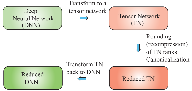
Figure 4.1: Optimization of Deep Neural Networks (DNNs) using the Tensor Network (TN) approach. In order to simplify a specific DNN and reduce the number of its parameters, we first transform the DNN into a specific TN, e.g., TT/MPS, then transform the so approximated (with reduced rank) TN back to a new, optimized DNN. Such a transformation can be performed in a layer by layer fashion, or globally for the whole DNN. Optionally, we may choose to first construct and learn (e.g., via tensor completion) a tensor network and then transform it to an equivalent DNN.

It should be noted that, in practice, the reduction of DNNs through low-rank TN approximations offers many potential advantages over a direct reduction of redundant DNNs, owing to the availability of many efficient optimization methods to reduce the number of parameters and achieve a pre-specified approximation error. Moreover, low-rank tensor networks are capable of avoiding the curse of dimensionality through low-order sparsely interconnected core tensors.

On the other hand, in the past two decades, quantum physicists and computer scientists have developed solid theoretical understanding and efficient numerical techniques for low-rank TN decompositions, especially the TT/MPS and TT/MPO. The entanglement entropy, Renyi’s entropy, entanglement spectrum and long-range correlations are the most widely used quantities (calculated from a spatial reduced density matrix) investigated in the theory of tensor networks. The spatial reduced density matrix is determined by splitting a TN into two parts, say, regions A and B, where a density matrix in region A is generated by integrating out all the degrees of freedom in region B. The entanglement spectra are determined by the eigenvalues of the reduced density matrix [Zwanziger, 1994, Eisert et al., 2010]. Entanglement entropy also characterizes the information content of a bipartition of a specific TN. Furthermore, the entanglement area law explains that the entanglement entropy increases only proportionally to the boundary between the two tensor sub-networks. Also, entanglement entropy characterizes the information content of the distribution of singular values of a matricized tensor, and can be viewed as a proxy for the correlations between the two partitions; uncorrelated data has zero entanglement entropy at any bipartition.

Note that TNs are usually designed to efficiently represent large systems which exhibit a relatively low entanglement entropy. In practice, similar to deep neural networks, we often need to only care about a small fraction of the input measurements or training data among a huge number of possible inputs. This all suggest that certain guiding principles in DNNs correspond to the entanglement area law used in the theory of tensor networks. These may then be used to quantify the expressive power of a wide class of DCNNs. Note that long range correlations also typically increase with the entanglement. We therefore conjecture that realistic datasets in most successful machine learning applications have relatively low entanglement entropies [Calabrese and Cardy, 2004]. On the other hand, by exploiting the entanglement entropy bound of TNs, we can rigorously quantify the expressive power of a wide class of DNNs applied to complex and highly correlated datasets.

4.2 Restricted Boltzmann Machines (RBM)

Restricted Boltzmann machines (RBMs), illustrated in Figure 4.2, are generative stochastic artificial neural networks, which have found a wide range of applications in dimensionality reduction, feature extractions, and recommender systems, by virtue of their inherent modeling of the probability distributions of a variety of input data, including natural image and speech signals.

The RBMs are fundamental basic building blocks in a class of Deep (restricted) Boltzmann Machines (DBMs) and Deep Belief Nets (DBNs). In such deep neural networks, after training one RBM layer, the values of its hidden units can be treated as data for training higher-level RBMs (see Figure 4.3).

To create an RBM, we first perform a partition of variables into at least two sets: visible (observed) variables, $\mathbf{v}\in\mathbb{R}^{M}$, and hidden variables, $\mathbf{h}\in\mathbb{R}^{K}$. The goal of RBMs is then to learn a higher-order latent representation, $\mathbf{h}\in\mathbb{R}^{K}$, typically for binary variables, within a bipartite undirected graphical model encoding these two layers, as illustrated in Figure 4.2(a).

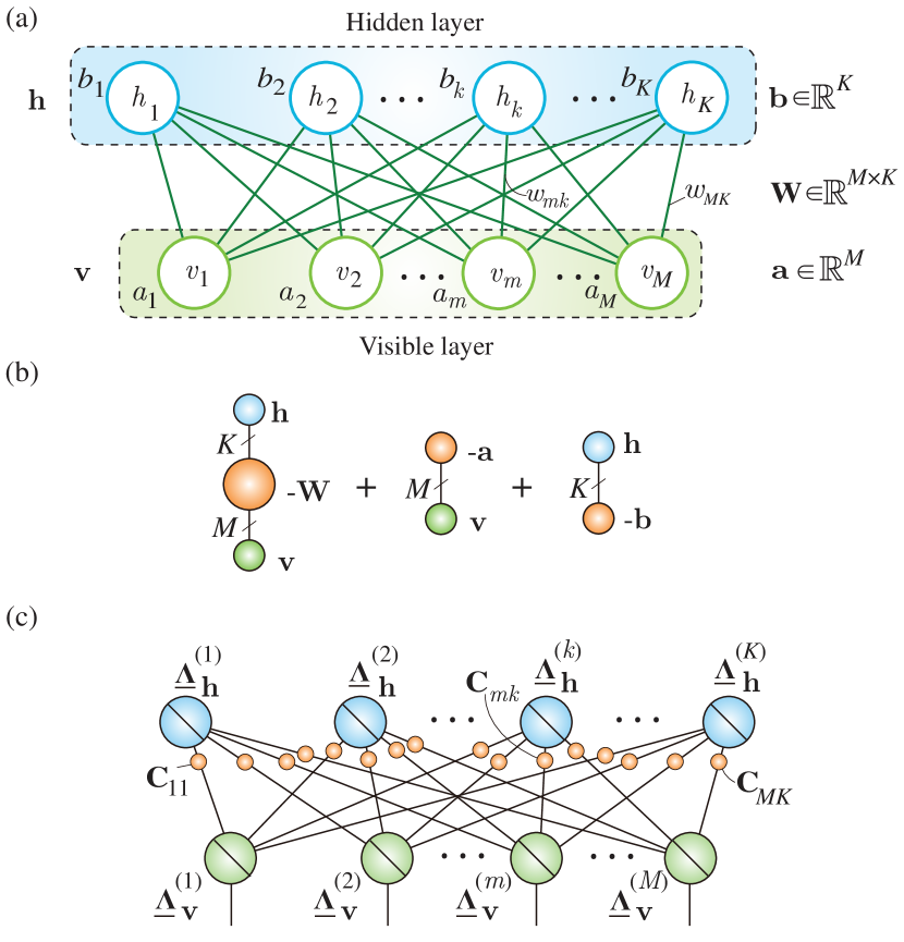
Figure 4.2: Graphical illustrations of the standard RBM. (a) Basic RBM model. The top (hidden) layer represents a vector ${\bf h}$ of stochastic binary variables, $h_{k}$ $(k=1,\ldots,K)$, and the bottom (visible) layer represents a vector, ${\bf v}$, of stochastic binary variables, $v_{m}$ $(m=1,\ldots,M)$. White round nodes represent observed (visible) and hidden variables while green lines show the links between the variables. (b) Energy function, $E({\bf v},{\bf h};\theta)=-{\bf v}^{\text{T}}{\bf W}{\bf h}-{\bf a}^{\text{T}}{\bf v}-{\bf b}^{\text{T}}{\bf h}$ for $\mathcal{F}({\bf v})=0$, represented by TN diagrams (see (4.1)). (c) A TN diagram corresponding to an RBM with diagonal core tensors, $\underline{\mbox{\boldmath$\Lambda$}}_{{\bf v}}^{(m)}=\mbox{diag}_{K}(1,e^{a_{m}})$ and $\underline{\mbox{\boldmath$\Lambda$}}_{{\bf h}}^{(k)}=\mbox{diag}_{M}(1,e^{b_{k}})$, and factor matrices, ${\bf C}_{mk}=[1,1;1,e^{w_{mk}}]$. The TN can be simplified through conversion to TT/MPS formats [Chen et al., 2017]. The tensor network represents a set of parameters $\theta=\{{\bf W},{\bf a},{\bf b}\}$. Large scale matrices and vectors can also be represented by a TT network, as explained in Chapter 3.

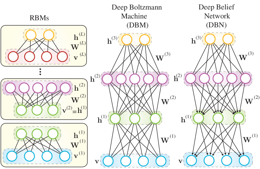
Figure 4.3: Graphical illustrations of the construction of Deep (restricted) Boltzmann Machines (DBMs) and Standard Deep Belief Networks (DBNs). Both use initialization schemes based on greedy layer-wise training of Restricted Boltzmann Machines (RBMs) (left panel), i.e., they are both probabilistic graphical models consisting of stacked layers of RBMs. Although DBNs and DBMs look diagrammatically quite similar, they are qualitatively very different. The main difference is in how the hidden layers are connected. In a DBM, the connection between all layers is undirected, thus each pair of layers forms an RBM, while a DBN has undirected connections between its top two layers and downward directed connections between all its lower layers (see Salakhutdinov and Hinton [2009] for detail).

The basic idea is that the hidden units of a trained RBM represent relevant features of observations. In other words, an RBM is a probabilistic graphical model based on a layer of hidden variables, which is used to build the probability distribution over input variables. The standard RBM assigns energy to a joint configuration $(\mathbf{v},\mathbf{h})$ as (see Figure 4.2(b))

$$E(\mathbf{v},\mathbf{h};\theta)=-(\mathcal{F}(\mathbf{v})+\mathbf{v}^{\text{T}}\mathbf{W}\mathbf{h}+\mathbf{a}^{\text{T}}\mathbf{v}+\mathbf{b}^{\text{T}}\mathbf{h}),$$ (4.1)

where $\mathbf{a}\in\mathbb{R}^{M}$ and $\mathbf{b}\in\mathbb{R}^{K}$ are the biases corresponding to the visible and hidden variables, $\mathbf{W}\in\mathbb{R}^{M\times K}$ is the (coupling) matrix of mapping parameters, $\theta=\{\mathbf{a},\mathbf{b},\mathbf{W}\}$ is a set of the model parameters to be estimated, and $\mathcal{F}(\mathbf{v})$ is a type-specific function, e.g., $\mathcal{F}(\mathbf{v})=0$ for a binary input and $\mathcal{F}(\mathbf{v})=-0.5\sum_{m}v_{m}^{2}$ for Gaussian variables. Such an RBM model obeys the Boltzmann distribution for binary variables, as follows

$$p(\mathbf{v},\mathbf{h}\;|\;\theta) = \frac{1}{Z(\theta)}\text{exp}\left(-E(\mathbf{v},\mathbf{h};\theta)\right),$$ (4.2)

where $Z(\theta)$ is the normalization constant.

The absence of connections between hidden binary variables within RBMs allows us to calculate relatively easily the marginal distribution of the visible variables, as follows

$$p({\bf v}\,|\,\theta) = \sum_{{\bf h}}p({\bf v},{\bf h}\,|\,\theta)=\frac{1}{Z}\sum_{{\bf h}}\exp\left({-E({\bf v},{\bf h};\theta})\right)$$

$$= \frac{1}{Z}\prod_{m=1}^{M}\exp\left(a_{m}v_{m}\right)\prod_{k=1}^{K}\left(1+\exp\left(b_{k}+\sum_{m=1}^{M}w_{mk}v_{m}\right)\right),$$

and the distribution of the hidden variables

$$p({\bf h}\;|\;\theta) = \sum_{{\bf v}}p({\bf v},{\bf h}\,|\,\theta)=\frac{1}{Z}\sum_{{\bf v}}\exp(-E(\mathbf{v},\mathbf{h};\theta))$$

$$= \frac{1}{Z}\exp\left(\sum_{k=1}^{K}b_{k}h_{k}\right)\prod_{m=1}^{M}\left(1+\exp\left(a_{m}+\sum_{k=1}^{K}w_{mk}h_{k}\right)\right).$$

The above formulas indicate that an RBM can be regarded as a product of “experts”, in which a number of experts for individual observations are combined multiplicatively [Fischer and Igel, 2012].

The RBM model can be converted into an equivalent (or corresponding) tensor network model. Figure 4.2(c) [Chen et al., 2017] shows that such a tensor network model comprises a set of interconnected diagonal core tensors: $K$th-order tensors $\underline{\mbox{\boldmath$\Lambda$}}^{(m)}_{{\bf v}}=\mbox{diag}_{K}(1,e^{a_{m}})$ and $M$th-order tensors $\underline{\mbox{\boldmath$\Lambda$}}^{(k)}_{{\bf h}}=\mbox{diag}_{M}(1,e^{b_{k}})$, all of sizes $2\times 2\times\cdots\times 2$. This means that the core tensors are extremely sparse since only the diagonal entries $\underline{\mbox{\boldmath$\Lambda$}}^{(m)}_{{\bf v}}(1,1,\ldots,1)=1$, $\underline{\mbox{\boldmath$\Lambda$}}^{(m)}_{{\bf v}}(2,2,\ldots,2)=e^{a_{m}}$, and $\underline{\mbox{\boldmath$\Lambda$}}^{(k)}_{{\bf h}}(1,1,\ldots,1)=1$ , $\underline{\mbox{\boldmath$\Lambda$}}^{(k)}_{{\bf h}}(2,2,\ldots,2)=e^{b_{k}}$ are non-zero. The diagonal core tensors in the visible and hidden layer are interconnected via the $2\times 2$ matrices ${\bf C}_{mk}=[1,1;1,e^{w_{mk}}]$.

The bipartite structure of the RBM enables units in one layer to become conditionally independent of the other layer. Thus, the conditional distributions over the hidden and visible variables can be factorized as

$$p(\mathbf{v}|\mathbf{h};\theta) =\prod_{m=1}^{M}p(v_{m}|\mathbf{h}),\quad p(\mathbf{h}|\mathbf{v};\theta) =\prod_{k=1}^{K}p(h_{k}|\mathbf{v}),$$ (4.5)

and

$$\begin{split}p(v_{m}=1|\mathbf{h})&=\sigma\left(\sum_{k}w_{mk}h_{k}+a_{m}\right),\\ p(h_{k}=1|\mathbf{v})&=\sigma\left(\sum_{m}w_{mk}v_{m}+b_{k}\right),\end{split}$$ (4.6)

where $\sigma(x)=1/(1+\text{exp}(-x))$ is the sigmoid function.

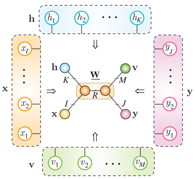
Figure 4.4: Energy function of a higher-order (multi-way) RBM with four layers, given in (4.7). In order to reduce the number of parameters, the 4th-order weight tensor $\underline{{\bf W}}\in\mathbb{R}^{I\times J\times M\times K}$ is represented in a distributed (tensor network) form, in this particular case as two 3rd-order cores. This allows us to reduce the number of parameters from $IJKM$ to only $IKR+JMR$, where typically $R\ll I,J,K,M$.

Higher-order RBMs. The modeling power of an RBM can be enhanced by increasing the number of hidden units, or by adding and splitting visible layers and/or adding conditional and activation layers. The standard RBM can be generalized and extended in many different ways. The most natural way is to jointly express the energy for more than two set of variables. For example, for four sets of binary variables, ${\bf v},{\bf h},{\bf x},{\bf y}$, the energy function (with neglected biases) can be expressed in the following form (see Figure 4.4)

$$E({\bf v},{\bf h},{\bf x},{\bf y}) = -\sum_{i=1}^{I}\sum_{j=1}^{J}\sum_{m=1}^{M}\sum_{k=1}^{K}w_{ijmk}\;x_{i}\,y_{j}\,v_{m}\,h_{k}$$ (4.7)

$$= -\underline{{\bf W}}\;\bar{\times}_{1}\;{\bf x}\;\bar{\times}_{2}\;{\bf y}\;\bar{\times}_{3}\;{\bf v}\;\bar{\times}_{4}{\bf h}.$$

Unfortunately, higher-order RBM models suffer from a large number of parameters, which scales with the product of visible, hidden and conditioning variables. To alleviate this problem, we can perform dimensionality reduction via low-rank tensor network approximations.

4.2.1 Matrix Variate Restricted Boltzmann Machines

The matrix-variate restricted Boltzmann machine (MVRBM) model was proposed as a generalization of the classic RBM to explicitly model matrix data [Qi et al., 2016], whereby both input and hidden variables are in their matrix forms which are connected by bilinear transforms. The MVRBM has much fewer model parameters than the standard RBM and thus admits faster training while retaining a comparable performance to the classic RBM.

Let $\mathbf{V}\in\mathbb{R}^{J\times M}$ be a binary matrix of visible variables, and $\mathbf{H}\in\mathbb{R}^{K\times I}$ a binary matrix of hidden variables. Given the parameters of a 4th-order tensor, $\underline{\mathbf{W}}\in\mathbb{R}^{I\times J\times M\times K}$, and bias matrices, ${\bf A}\in\mathbb{R}^{J\times M}$ and ${\bf B}\in\mathbb{R}^{K\times I}$, the energy function can be defined as (see Figure 4.5)

$$E(\mathbf{V},\mathbf{H};\theta) = -\sum_{i=1}^{I}\sum_{j=1}^{J}\sum_{m=1}^{M}\sum_{k=1}^{K}v_{mj}w_{ijmk}h_{ki}$$

$$-\sum_{m=1}^{M}\sum_{j=1}^{J}v_{jm}a_{jm}-\sum_{k=1}^{K}\sum_{i=1}^{I}h_{ki}b_{ki},$$

where $\theta=\{\underline{\mathbf{W}},{\bf A},{\bf B}\}$ is the set of all model parameters.

In order to reduce the number of free parameters, the higher-order weight tensor can be approximated by a suitable tensor network, e.g. a TT or HT network. In the particular case of a four-way weight tensor, $\underline{{\bf W}}\in\mathbb{R}^{I\times J\times M\times K}$, it can be represented via truncated SVD by two 3rd-order core tensors, $\underline{{\bf W}}^{(1)}\in\mathbb{R}^{M\times K\times R}$ and $\underline{{\bf W}}^{(2)}\in\mathbb{R}^{I\times J\times R}$. For a very crude approximation with rank $R=1$, these core tensors simplify to matrices ${\bf W}^{(1)}\in\mathbb{R}^{M\times K}$ and ${\bf W}^{(2)}\in\mathbb{R}^{I\times J}$, while the energy function in (4.2.1) simplifies to the following form

$$E(\mathbf{V},\mathbf{H};\theta)=-\text{tr}({\bf W}^{(1)}\mathbf{H}{\bf W}^{(2)}\mathbf{V})-\text{tr}(\mathbf{V}^{\text{T}}\mathbf{A})-\text{tr}(\mathbf{H}^{\text{T}}{\bf B}).$$ (4.9)

Both matrices ${\bf W}^{(1)}$ and ${\bf W}^{(2)}$ approximate the interaction between the input matrix $\mathbf{V}$ and the hidden matrix $\mathbf{H}$. Note that in this way, the total number of free parameters is reduced from $IJMK$ to $IJ+KM+JM+IK$. For the corresponding learning algorithms see Salakhutdinov and Hinton [2009], Fischer and Igel [2012], Qi et al. [2016].

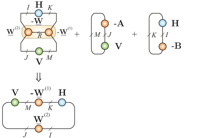
Figure 4.5: Energy function of the matrix-variate RBM represented by TN diagrams, given in (4.2.1). In order to reduce the number of parameters, the 4th-order weight tensor can be represented by the outer product of two matrices (lower panel), $\underline{{\bf W}}={\bf W}^{(1)}\circ{\bf W}^{(2)}$. For a higher order weight tensor, we can use the low-rank TT or HT representations.

4.2.2 Tensor-Variate Restricted Boltzmann Machines

The tensor-variate RMBs (TvRBMs) have the ability to capture multiplicative interactions between data modes and latent variables (see e.g. [Nguyen et al., 2015]). The TvRBMs are highly compact, in that the number of free parameters grows only linearly with the number of modes, while their multiway factoring of mapping parameters link data modes and hidden units. Modes interact in a multiplicative fashion gated by hidden units, and TvRBM uses tensor data and the hidden layer to construct an ($N+1$)-mode tensor.

In a TvRBM, the set of visible units is represented by an $N$th-order tensor, $\underline{\mathbf{V}}\in\mathbb{R}^{I_{1}\times I_{2}\times\cdots\times I_{N}}$, and the hidden units $\mathbf{h}$ are the same as in RBM. The goal is to model the joint distribution, $p(\underline{\mathbf{V}},\mathbf{h})$, by the optimization of the energy function

$$E(\underline{\mathbf{V}},\mathbf{h};\mbox{\boldmath$\theta$})=-\mathcal{F}(\underline{\mathbf{V}})-\langle\underline{\mathbf{A}},\underline{\mathbf{V}}\rangle-\mathbf{b}^{\text{T}}\mathbf{h}-\langle\underline{\mathbf{W}},\underline{\mathbf{V}}\circ{\bf h}\rangle,$$ (4.10)

where $\mathcal{F}(\underline{\mathbf{V}})$ is a type-specific function, $\underline{\mathbf{A}}\in\mathbb{R}^{I_{1}\times I_{2}\times\cdots\times I_{N}}$ are visible biases, and $\underline{\mathbf{W}}\in\mathbb{R}^{I_{1}\times I_{2}\times\cdots\times I_{N}\times K}$ are mapping parameters.

The hidden posterior is then given by

$$p(h_{k}=1|\underline{\mathbf{V}};\theta)=\sigma\left(b_{k}+\langle\underline{\mathbf{V}},\underline{\mathbf{W}}(:,\ldots,:,k)\rangle\right),$$ (4.11)

where $\sigma(x)$ is the sigmoid function. The generative distribution, $p(\underline{\mathbf{V}}|\mathbf{h})$, on the other hand is type-specific.

The most popular cases are the binary and Gaussian inputs. For a binary input, we have $\mathcal{F}(\underline{\mathbf{V}})=0$, and the following generative distribution

$$p(v_{i_{1}i_{2}\ldots i_{N}}|\mathbf{h})=\sigma\left(a_{i_{1}i_{2}\ldots i_{N}}+\underline{\mathbf{W}}(i_{1},\ldots,i_{N},:)^{\text{T}}\;{\bf h}\right).$$ (4.12)

For a Gaussian input, assuming unit variance, i.e. $\mathcal{F}(\underline{\mathbf{V}})=-0.5\langle\underline{\mathbf{V}},\underline{\mathbf{V}}\rangle$, the generative distribution becomes

$$p(v_{i_{1}i_{2}\ldots i_{N}}|\mathbf{h})=\mathcal{N}\left(\{a_{i_{1}i_{2}\ldots i_{n}}+\underline{\mathbf{W}}(i_{1},\ldots,i_{N},:)^{\text{T}}\;{\bf h}\};\underline{\mathbf{1}}\right),$$ (4.13)

where $\underline{\mathbf{1}}\in\mathbb{R}^{I_{1}\times I_{2}\times\cdots\times I_{N}}$ is the tensor with unit elements.

A major problem with the parameterizations of $\underline{\mathbf{W}}$ is the excessively large number of free parameters, which scales with the product of data modes and hidden dimensions. In particular, the $(N+1)$th-order weight tensor $\underline{\mathbf{W}}$ has $K\prod_{n}I_{n}$ elements, and its size quickly reaches billions of entries, even when the mode dimensionalities $K,(I_{1},\ldots,I_{N})$ and $N$ are quite moderate. This makes learning in the raw tensor format extremely difficult or even impossible, since robust estimation of parameters would require a huge dataset. To this end, low-rank tensor network decompositions can be employed to construct approximate interactions between visible modes and hidden units.

In the simplest scenario, we can approximately represent $\underline{\mathbf{W}}$ by a rank-$R$ CP tensor

$$\underline{\mathbf{W}} = \sum_{r=1}^{R}\lambda_{r}\cdot(\mathbf{w}_{r}^{(1)}\circ\cdots\circ\mathbf{w}_{r}^{(N)}\circ\mathbf{w}_{r}^{(N+1)})$$

$$= \underline{\mbox{\boldmath$\Lambda$}}\times_{1}{\bf W}^{(1)}\cdots\times_{N}{\bf W}^{(N)}\times_{N+1}{\bf W}^{(N+1)},$$

where the matrix ${\bf W}^{(n)}=[{\bf w}_{1}^{(n)},\ldots,{\bf w}^{(n)}_{R}]\in\mathbb{R}^{I_{n}\times R}$ for $n=1,\ldots,N$ represents the mode-factor weights, and ${\bf W}^{(N+1)}={\bf W}^{(h)}\in\mathbb{R}^{K\times R}$ the hidden-factor matrix. Such factoring allows for multiplicative interactions between modes to be moderated by the hidden units through the hidden-factor matrix $\mathbf{W}^{(h)}$. Thus, the model captures the modes of variation through the new representation, enabled by $\mathbf{h}$. By employing the CP decomposition, the number of mapping parameters may be reduced down to $R(K+\sum_{n}I_{n})$, which grows linearly rather than exponentially in $N$. Importantly, the conditional independence among intra-layer variables, i.e. $p(\mathbf{h}|\underline{\mathbf{V}})=\prod_{k=1}^{K}p(h_{k}|\underline{\mathbf{V}})$ and $p(\underline{\mathbf{V}}|\mathbf{h})=\prod_{n}\prod_{i_{n}=1}^{I_{n}}p(v_{i_{1}i_{2}\ldots i_{N}}|\mathbf{h})$, is not affected. Therefore, the model preserves the fast sampling and interface properties of RBM.

4.3 Basic Features of Deep Convolutional Neural Networks

Basic DCNNs are characterized by at least three features: locality, weight sharing (optional) and pooling, as explained below:

• Locality refers to the connection of a (artificial) neuron to only neighboring neurons in the preceding layer, as opposed to being fed by the entire layer (this is consistent with biological NNs).

• Weight sharing reflects the property that different neurons in the same layer, connected to different neighborhoods in the preceding layer, often share the same weights. Note that weight sharing, when combined with locality, gives rise to standard convolution.

• Pooling is essentially an operator which gradually decimates (reduces) layer sizes by replacing the local population of neural activations in a spatial window by a single value (e.g., by taking their maxima, average values or their scaled products). In the context of images, pooling induces invariance to translation, which often does not affect semantic content, and is interpreted as a way to create a hierarchy of abstractions in the patterns that neurons respond to [Anselmi et al., 2015, Cohen et al., 2016].

Usually, DCNNs perform much better when dealing with compositional function approximations and multi-class classification problems than shallow neural network architectures with one hidden layer. In fact, DCNNs can even efficiently and conveniently select a subset of features for multiple classes, while for efficient learning a DCNN model can be pre-trained by first learning each DCNN layer, followed by fine tuning of the parameter of the entire model, using e.g., stochastic gradient descent. To summarize, deep learning neural networks have the ability to arbitrarily well exploit and approximate the complexity of compositional hierarchical functions, a wide class of functions to which shallow networks are blind.

4.4 Score Functions for Deep Convolutional Neural Networks

Consider a multi-class classification task where the input training data, also called local structures or instances, e.g., input patches in images, are denoted by the set $X=\{{\bf x}_{1},\ldots,{\bf x}_{N}\}$, where ${\bf x}_{n}\in\mathbb{R}^{S}$, $\;(n=1,\ldots,N)$, belong to one of distinct categories (classes) denoted by $c\in\{1,2,\ldots,C\}$. Such a representation is quite natural for many high-dimensional data – in images, the local structures represent vectorization of patches consisting of $S$ pixels, while in audio data can be represented through spectrograms.

For this kind of problems, DCNNs can be described by a set of multivariate score functions

$$y=h_{c}({\bf x}_{1},\ldots,{\bf x}_{N})=\sum_{i_{1}=1}^{I_{1}}\cdots\sum_{i_{N}=1}^{I_{N}}\underline{{\bf W}}_{\,c}(i_{1},\ldots,i_{N})\prod_{n=1}^{N}f_{\theta_{i_{n}}}({\bf x}_{n}),$$

(4.15)

where $\underline{{\bf W}}_{\,c}\in\mathbb{R}^{I_{1}\times\cdots\times I_{N}}$ is an $N$th-order coefficient tensor, with all dimensions $I_{n}=I,\;\forall n$, $N$ is the number of (overlapped) input patches $\{{\bf x}_{n}\}$, $I_{n}$ is the size (dimension) of each mode $\underline{{\bf W}}_{\,c}$, and $f_{\theta_{1}},\ldots,f_{\theta_{I_{n}}}$ are referred to as the representation functions (in the representation layer) selected from a parametric family of nonlinear functions.

In general, the one-dimensional basis functions could be polynomials, splines or other sets of basis functions. Natural choices for this family of nonlinear functions are also radial basis functions (Gaussian RBFs), wavelets, and affine functions followed by point-wise activations. Note that the representation functions in standard (artificial) neurons have the form

$$f_{\theta_{i}}({\bf x})=\sigma(\tilde{\bf w}_{i}^{\text{T}}{\bf x}+b_{i}),$$ (4.16)

for the set of parameters $\theta_{i}=\{\tilde{\bf w}_{i},b_{i}\}$, where $\sigma(\cdot)$ is a suitably chosen activation function.

(a)                                     (b)                            (c)

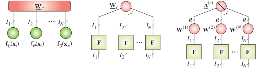
Figure 4.6: Various representations of the score function of a DCNN. (a) Direct representation of the score function $h_{c}({\bf x}_{1},{\bf x}_{2},\ldots,{\bf x}_{N})=\underline{\mathbf{W}}_{c}\bar{\times}_{1}{{\bf f}}_{\mbox{\boldmath$\theta$}}({\bf x}_{1})\bar{\times}_{2}{{\bf f}}_{\mbox{\boldmath$\theta$}}({\bf x}_{2})\cdots\bar{\times}_{N}{{\bf f}}_{\mbox{\boldmath$\theta$}}({\bf x}_{N})$. (b) Graphical illustration of the $N$th-order grid tensor of the score function $h_{c}$, which can be considered as a special case of Tucker-$N$ model where the representation matrix ${\bf F}\in\mathbb{R}^{I\times I}$ is built up of factor matrices; note that all the factor matrices are the same and $I_{n}=I,\;\forall n$. (c) CP decomposition of the coefficient tensor $\underline{{\bf W}}_{\,c}=\underline{\mbox{\boldmath$\Lambda$}}^{(c)}\times_{1}{\bf W}^{(1)}\times_{2}{\bf W}^{(2)}\cdots\times_{N}{\bf W}^{(N)}=\sum_{r=1}^{R}\lambda^{(c)}_{r}\;({\bf w}^{(1)}_{r}\circ{\bf w}^{(2)}_{r}\circ\cdots\circ{\bf w}^{(N)}_{r})$, where ${\bf W}^{(n)}=[{\bf w}^{(n)}_{1},\ldots,{\bf w}^{(n)}_{R}]\in\mathbb{R}^{I\times R}$. This CP model corresponds to a simple shallow neural network with one hidden layer comprising weights $w^{(n)}_{ir}$, and the output layer comprising weights $\lambda^{(c)}_{r}$, $r=1,\ldots,R$. Note that the coefficient tensor $\underline{{\bf W}}_{c}$ can be represented in a distributed form by any suitable tensor network.

The representation layer play a key role to transform the inputs, by means of $I$ nonlinear functions, $f_{\theta_{i}}({\bf x}_{n})$ $\;(i=1,2,\ldots,I)$, to template input patches, thereby creating $I$ feature maps [Cohen and Shashua, 2016]. Note that the representation layer can be described by a feature vector defined as

$${{\bf f}}={{\bf f}}_{\mbox{\boldmath$\theta$}}({\bf x}_{1})\otimes{{\bf f}}_{\mbox{\boldmath$\theta$}}({\bf x}_{2})\otimes\cdots\otimes{{\bf f}}_{\mbox{\boldmath$\theta$}}({\bf x}_{N})\in\mathbb{R}^{I_{1}I_{2}\cdots I_{N}},$$ (4.17)

where ${{\bf f}}_{\mbox{\boldmath$\theta$}}({\bf x}_{n})=[f_{\theta_{1}}({\bf x}_{n}),f_{\theta_{2}}({\bf x}_{n}),\ldots,f_{\theta_{I_{n}}}({\bf x}_{n})]^{T}\in\mathbb{R}^{I_{n}}$ for $n=1,2,\ldots,N$ and $i_{n}=1,2,\ldots,I_{n}$. Equivalently, the representation layer can be described as a rank one tensor (see Figure 4.6(a))

$$\underline{{\bf F}}={{\bf f}}_{\mbox{\boldmath$\theta$}}({\bf x}_{1})\circ{{\bf f}}_{\mbox{\boldmath$\theta$}}({\bf x}_{2})\circ\cdots\circ{{\bf f}}_{\mbox{\boldmath$\theta$}}({\bf x}_{N})\in\mathbb{R}^{I_{1}\times I_{2}\times\cdots\times I_{N}}.$$ (4.18)

This allows us to represent the score function as an inner product of two tensors, as illustrated in Figure 4.6(a)

$$h_{c}({\bf x}_{1},\ldots,{\bf x}_{N})=\langle\underline{\mathbf{W}}_{c},\underline{\mathbf{F}}\rangle=\underline{\mathbf{W}}_{c}\;\bar{\times}_{1}\;{{\bf f}}_{\mbox{\boldmath$\theta$}}({\bf x}_{1})\;\bar{\times}_{2}\;{{\bf f}}_{\mbox{\boldmath$\theta$}}({\bf x}_{2})\cdots\bar{\times}_{N}\;{{\bf f}}_{\mbox{\boldmath$\theta$}}({\bf x}_{N}).$$

To simplify the notations, assume that $I_{n}=I,\;\forall n$, then we can also construct a square matrix ${\bf F}\in\mathbb{R}^{I\times I}$ , with rows ${\bf F}(i,:)=[f_{\theta_{1}}({\bf x}^{(i)}),f_{\theta_{2}}({\bf x}^{(i)}),\ldots,f_{\theta_{I}}({\bf x}^{(i)})]$ for $i=1,2,\ldots,I$ and entries taken from values of nonlinear basis functions $\{f_{\theta_{1}},\ldots,f_{\theta_{I}}\}$ on the selected templates $\{{\bf x}^{(1)},{\bf x}^{(2)},\ldots,{\bf x}^{(I)}\}$ [Cohen and Shashua, 2016].

For discrete data values, the score function can be represented by a grid tensor, as graphically illustrated in Figure 4.6(b). The grid tensor of the nonlinear score function $h_{c}({\bf x}_{1},,...,{\bf x}_{N})$ determined over all the templates ${\bf x}^{(1)},{\bf x}^{(2)},...,{\bf x}^{(I)}$ can be expressed, as follows

$$\underline{\mathbf{W}}(h_{c})=\underline{\mathbf{W}}_{c}\times_{1}{\bf F}\times_{2}{\bf F}\cdots\times_{N}{\bf F}.$$ (4.20)

Of course, since the order $N$ of the coefficient (core) tensor is large, it cannot be implemented, or even saved on a computer due to the curse of dimensionality.

To this end, we represent the weight tensor in some low-rank tensor network format with a smaller number of parameters. A simple model is the CP representation, which leads to a shallow network as illustrated in Figure 4.6(c). However, this approach is associated with two problems: (i) the rank $R$ of the coefficient tensor $\underline{\mathbf{W}}_{c}$ can be very large (so compression ratio cannot be very high), (ii) the existing CP decomposition algorithms are not very stable for very high-order tensors, and so an alternative promising approach would be to apply tensor networks such as HT that enable us to avoid the curse of dimensionality.

Following the representation layer, a DCNN may consists of a cascade of $L$ convolutional hidden layers with pooling in-between, where the number of layers $L$ should be at least two. In other words, each hidden layer performs 3D or 4D convolution followed by spatial window pooling, in order to reduce (decimate) feature maps by e.g., taking a product of the entries in sub-windows. The output layer is a linear dense layer.

Classification can then be carried out in a standard way, through the maximization of a set of labeled score functions, $h_{c}$ for $C$ classes, that is, the predicted label for the input instants $X=({\bf x}_{1},\ldots,{\bf x}_{N})$ will be the index $\hat{y}$ for which the score value attains a maximum, that is

$$\hat{y}=\displaystyle{\mbox{argmax}_{\{c\}}}h_{c}({\bf x}_{1},\ldots,{\bf x}_{N}).$$ (4.21)

Such score functions can be represented through their coefficient tensors which, in turn, can be approximated by low-rank tensor network decompositions.

One restriction of the so formulated score functions (4.15) is that they allow for a straightforward implementation of only a particular class of DCNNs, called convolutional Arithmetic Circuit (ConvAC). However, the score functions can be approximated indirectly and almost equivalently using more popular CNNs (see the next section). For example, it was shown recently how NNs with a univariate rectified linear unit (ReLU) nonlinearity may perform multivariate function approximation [Poggio et al., 2016].

As discussed in Part 1 and in Chapter 1 the main idea is to employ a low-rank tensor network representation to approximate and interpolate a multivariate function $h_{c}({\bf x}_{1},\ldots,{\bf x}_{N})$ of $N$ variables by a finite sum of separated products of simpler functions (i.e., via sparsely interconnected core tensors).

Tensorial Mixture Model (TMM). Recently, the model in (4.15) has been extended to a corresponding probabilistic model, referred to as the Tensorial Mixture Model (TMM), given by Sharir et al. [2016]

$$P({\bf x}_{1},{\bf x}_{2},\ldots, {\bf x}_{N} |\;y=c)$$

$$= \sum_{i_{1}=1}^{I}\cdots\sum_{i_{N}=1}^{I}\underline{{\bf P}}_{y=c}(i_{1},\ldots,i_{N})\prod_{n=1}^{N}P({\bf x}_{n}|i_{n};\theta_{i_{n}}),$$

where $\underline{{\bf P}}_{(y=c)}(i_{1},\ldots,i_{N})$ (corresponding to $\underline{{\bf W}}_{\,c}(i_{1},\ldots,i_{N})$) are jointly decomposed prior tensors and $\{P({\bf x}_{n}|i_{n};\theta_{i_{n}})\}$ (corresponding to $f_{\theta_{i_{n}}}({\bf x}_{n})$) are mixing components (marginal likelihoods) shared across all input samples ${\bf x}_{n}$ $(n=1,\ldots,N)$ and classes $\{c\}$, $(c=1,2,\ldots,C)$. Note that for computational tractability, suitable scaling and nonnegativity constraints must be imposed on the TMM model.

The TMM can be considered as a generalization of standard mixture models widely used in machine learning, such as the Gaussian Mixture Model (GMM). However, unlike the standard mixture models, in the TMM we cannot perform inference directly from (4.4), nor can we even store the prior tensor, $\underline{{\bf P}}_{(y=c)}(i_{1},\ldots,i_{N})\in\mathbb{R}^{I\times\cdots\times I}$, given its exponential size of $I^{N}$ entries. Therefore, the TMM presented by (4.4) is not tractable directly but only in a distributed form, whereby the coefficient tensor is approximated by low-rank tensor network decompositions with non-negative cores. The TMM based on the HT decompositions is promising for multiple classification problems with partially missing training data, and potentially even regardless of the distribution of missing data [Sharir et al., 2016].

4.5 Convolutional Arithmetic Circuits and HT Networks

Conceptually, the Convolutional Arithmetic Circuit (ConvAC) can be divided into three parts: (i) the first (input) layer is the representation layer which transforms input vectors $({\bf x}_{1},\ldots,{\bf x}_{N})$ into $N\,I$ real valued scalars $\{f_{\theta_{i}}({\bf x}_{n})\}$ for $n=1,\ldots,N$ and $i=1,\ldots,I$. In other words, the representation functions, $f_{\theta_{i}}:\mathbb{R}^{S}\rightarrow\mathbb{R}$, $i=1,\ldots,I$, map each local patch ${\bf x}_{n}$ into a feature space of dimension $I$; (ii) the second, a key part, is a convolutional arithmetic circuit consisting of many hidden layers that takes the $N\,I$ measurements (training samples) generated by the representation layer; (iii) the output layer, which can be represented by a matrix, $\underline{\mathbf{W}}^{(L)}\in\mathbb{R}^{R\times C}$, which computes $C$ different score functions $h_{c}$ [Cohen et al., 2016].

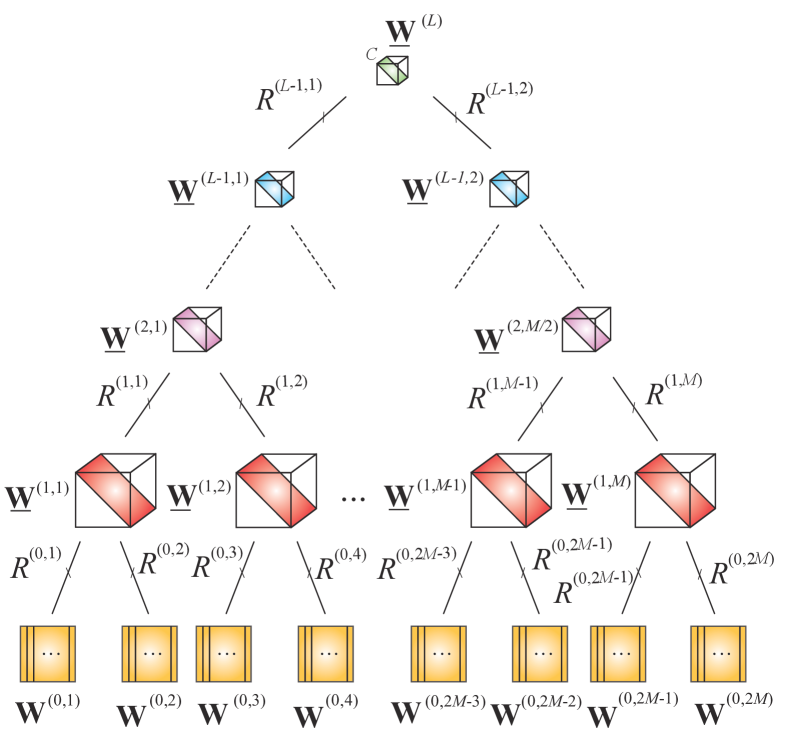
Figure 4.7: Architecture of a simplified Hierarchical Tucker (HT) network consisting of core tensors, $\underline{\mathbf{W}}^{(l,j)}$, with diagonal frontal slices, which approximates a grid tensor for a set of score functions $\{h_{c}\}$, for $c=1,\ldots,C$. This model corresponds to a ConvAC deep learning network. The HT tensor network consists of $L=\log_{2}(N)$ hidden layers with pooling-2 windows. For simplicity, we assumed $N=2M=2^{L}$ input patches, and equal HT-ranks $R^{(l,j)}$ in each layer, i.e., $R^{(l,1)}=R^{(l,2)}=\cdots=R^{(l)}$ for $l=0,1,\ldots,L-1$. Moreover, the cores have non-zero entries only on the diagonal of tensor cubes, as indicated by red rectangles. The representation layer is not explicitly shown.

Once the set of score functions has been formulated as (4.15), we can construct (design) a suitable multilayered or distributed representation for DCNN representation. The objective is to estimate the parameters $\theta_{1},\ldots,\theta_{I}$ and coefficient tensors $\underline{{\bf W}}_{\,1},\ldots,\underline{{\bf W}}_{\,C}$. Since the tensors are of $N$th-order and each with $I^{N}$ entries, in order to avoid the curse of dimensionality we employ low-rank tensor network representations. Note that a direct implementation of (4.15) or (4.4) is intractable owing to a huge number of parameters.

The simplified HT tensor network, shown in Figure 4.7, contains sparse 3rd-order core tensors $\underline{{\bf W}}^{(l,j)}\in\mathbb{R}^{R^{(l-1,2j-1)}\times R^{(l-1,2j-1)}\times R^{(l,j)}}$ for $l=1,\ldots,L-1$ and matrices ${\bf W}^{(0,j)}=[{\bf w}_{1}^{(0,j)},\ldots,{\bf w}_{R^{(0,j)}}^{(0,j)}]\in\mathbb{R}^{I_{j}\times R^{(0,j)}}$ for $l=0$ and $j=1,\ldots,N/2^{\,l}$ (for simplicity, we assumed that $N=2M=2^{L}$). In order to mimic basic features of the standard ConvAC, we assumed that $R^{(l,j)}=R^{(l)},\;\forall j$ and that frontal slices of the core tensors $\underline{{\bf W}}^{(l,j)}$ are diagonal matrices, with entries $\underline{\mathbf{W}}^{(l,j)}(r^{(l-1)},r^{(l-1)},r^{(l)})=w^{(l,j)}_{r^{(l-1)},r^{(l)}}$, as illustrated in Figure 4.7. The top (output) layer is represented by a 3rd-order tensor $\underline{\mathbf{W}}^{(L)}\in\mathbb{R}^{R^{(L-1)}\times R^{(L-1)}\times C}$ with diagonal frontal slices $\underline{\mathbf{W}}^{(L)}(:,:,c)=\mbox{diag}\{\lambda^{(c)}_{1},\ldots,\lambda^{(c)}_{R^{(L-1)}}\}$, $c=1,\ldots,C$. Note that the sparse core tensors $\underline{{\bf W}}^{(l,j)}$, with diagonal frontal slices, can be represented by dense matrices defined as ${\bf W}^{(l,j)}\in\mathbb{R}^{R^{(l-1)}\times R^{(l)}}$ for $l=1,\ldots,L-1$, and the top tensor can be also represented by a dense matrix ${\bf W}^{(L)}$ of size $R^{(L-1)}\times C$, in which each column corresponds to the diagonal matrix $\mbox{\boldmath$\lambda$}^{(c)}=\mbox{diag}\{\lambda^{(c)}_{1},\ldots,\lambda^{(c)}_{R^{(L-1)}}\}$.

The so simplified HT tensor network can be mathematically described in the following recursive form

$${\bf W}^{(0,j)} =[{\bf w}_{1}^{(0,j)},\ldots,{\bf w}^{(0,j)}_{R^{(0)}}]\in\mathbb{R}^{I_{j}\times R^{(0)}}$$

$${\bf W}^{(\leq 1,j)}_{r^{(1)}} =\sum_{r^{(0)}=1}^{R^{(0)}}w^{(1,j)}_{r^{(0)},r^{(1)}}\cdot\left({\bf w}^{(0,2j-1)}_{r^{(0)}}\circ{\bf w}^{(0,2j)}_{r^{(0)}}\right)\in\mathbb{R}^{I_{2j-1}\times I_{2j}}$$

$$\cdots$$ (4.23)

$$\underline{{\bf W}}^{(\leq l,j)}_{\;r^{(l)}} =\sum_{r^{(l-1)}=1}^{R^{(l-1)}}w^{(l,j)}_{r^{(l-1)},r^{(l)}}\cdot\left(\underline{{\bf W}}^{(\leq l-1,2j-1)}_{\;r^{(l-1)}}\circ\underline{{\bf W}}^{(\leq l-1,2j)}_{\;r^{(l-1)}}\right)$$

$$\cdots$$

$$\underline{{\bf W}}^{(\leq L-1,j)}_{r^{(L-1)}} =\sum_{r^{(L-2)}=1}^{R^{(L-2)}}w^{(L-1,j)}_{r^{(L-2)},r^{(L-1)}}\cdot\left(\underline{{\bf W}}^{(\leq L-2,2j-1)}_{\;r^{(L-2)}}\circ\underline{{\bf W}}^{(\leq L-2,2j)}_{\;r^{(L-2)}}\right)$$

for $j=1,\ldots,2^{L-l}$ and

$$\underline{{\bf W}}_{c} =\sum_{r^{(L-1)}=1}^{R^{(L-1)}}\lambda^{(c)}_{r^{(L-1)}}\cdot\left(\underline{{\bf W}}^{(\leq L-1,1)}_{\;r^{(L-1)}}\circ\underline{{\bf W}}^{(\leq L-1,2)}_{\;r^{(L-1)}}\right)\in\mathbb{R}^{I_{1}\times\cdots\times I_{N}},$$

where $\lambda^{(c)}_{r^{(L-1)}}=\underline{\mathbf{W}}^{(L)}(r^{(L-1)},r^{(L-1)},c)$.

In a special case, when the weights in each layer are shared, i.e., ${\bf W}^{(l,j)}={\bf W}^{(l)},\;\;\forall j$, the above equation can be considerably simplified to

$$\underline{{\bf W}}^{(\leq l)}_{r^{(l)}}=\sum_{r^{(l-1)}=1}^{R^{(l-1)}}w^{(l)}_{r^{(l-1)},r^{(l)}}\;(\underline{{\bf W}}^{(\leq l-1)}_{r^{(l-1)}}\circ\underline{{\bf W}}^{(\leq l-1)}_{r^{(l-1)}})$$ (4.25)

for the layers $l=1,\ldots,L$, where $\underline{{\bf W}}^{(\leq l)}_{r^{(l)}}=\underline{{\bf W}}^{(\leq l)}(:,\ldots,:,r^{(l)})\in\mathbb{R}^{I\times\cdots\times I}$ are sub-tensors of $\underline{{\bf W}}^{(\leq l)}$, for each $r^{(l)}=1,\ldots,R^{(l)}$, and $w^{(l)}_{r^{(l-1)},r^{(l)}}$ is the $(r^{(l-1)},r^{(l)})$th entry of the weight matrix ${\bf W}^{(l)}\in\mathbb{R}^{R^{(l-1)}\times R^{(l)}}$.

However, it should be noted that the simplified HT model shown in Figure 4.7 has a limited ability to approximate an arbitrary grid tensor, $\underline{{\bf W}}(h_{c})$, due to the strong constraints imposed on core tensors. A more flexible and powerful HT model is shown in Figure 4.8, in which the constraints imposed on 3rd-order cores have been completely removed. In fact this is the standard HT tensor network, which can be mathematically expressed as (with a slight abuse of notation), as follows

$${\bf w}^{(\leq 0,j)}_{r} = {\bf w}^{(0,j)}_{r}$$

$$\underline{{\bf W}}^{(\leq l,j)}_{\;r} = \sum_{r_{1}=1}^{R^{(l-1,2j-1)}}\sum_{r_{2}=1}^{R^{(l-1,2j)}}w^{(l,j)}_{r_{1},r_{2},r}\cdot\left(\underline{{\bf W}}^{(\leq l-1,2j-1)}_{\;r_{1}}\circ\underline{{\bf W}}^{(\leq l-1,2j)}_{\;r_{2}}\right)$$

$$\underline{{\bf W}}_{\,c} = \underline{{\bf W}}^{(\leq L,1)},$$

for $l=1,\ldots,L$ and $\;\;j=1,\ldots,2^{L-l}$.

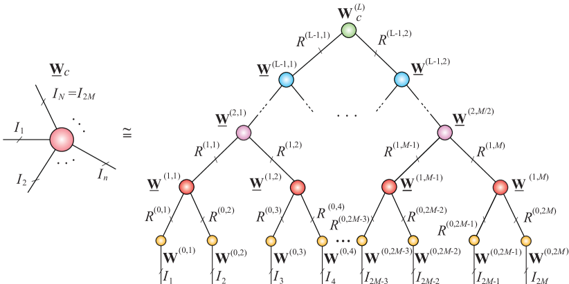
Figure 4.8: Hierarchical Tucker (HT) unconstrained tensor network for the distributed representation and/or approximation of coefficient tensors, $\underline{{\bf W}}_{\,c}$, of the score functions $h_{c}({\bf x}_{1},\ldots,{\bf x}_{N})$. In general, no constraints are imposed on core tensors. The representation layer is not explicitly shown. For a grid tensor of the set of score functions, the matrices ${\bf W}^{(L)}_{c}$ for $c=1,\ldots,C$ build up a 3rd-order tensor corresponding to the output layer.

The HT model can be further extended by using more flexible and general Tree Tensor Networks States (TTNS). As illustrated in Figure 4.9, the use of the TTNS, instead HT tensor networks, allows for more flexibility in the choice of the size of pooling-window, as the pooling size in each hidden layer can be adjusted by applying core tensors with a suitable variable order in each layer. For example, if we use 5th-order (4rd-order) core tensors instead 3rd-order cores, then the pooling layer will employ a size-4 pooling window (size-3 pooling) instead of only size-2 pooling window when using 3rd-order core tensors in HT tensor networks. For more detail regrading HT networks and their generalizations to TTNS, see Part 1 of our monograph [Cichocki et al., 2016].

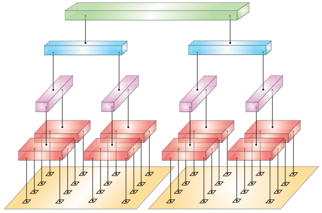
Figure 4.9: Tree Tensor Networks States (TTNS) with a variable order of core tensors. The rectangular prisms represent core tensors of orders 5 and 3, that allow pooling with the respective window sizes of 4 and 2. The first hidden layer comprises 5th-order cores, while the second and third layer consist of 3rd-order cores.

4.6 Convolutional Rectifier NN Using Nonlinear TNs

The convolutional arithmetic circuit (ConvACs) model employs the standard outer (tensor) products, which for two tensors, $\underline{{\bf A}}\in\mathbb{R}^{I_{1}\times\cdots\times I_{N}}$ and $\underline{{\bf B}}\in\mathbb{R}^{J_{1}\times\cdots\times J_{M}}$, are defined as

$$(\underline{{\bf A}}\circ\underline{{\bf B}})_{i_{1},\ldots,i_{N},j_{1},\ldots,j_{M}}=a_{i_{1},\ldots,i_{N}}\cdot b_{j_{1},\ldots,j_{M}}.$$

In order to convert ConvAC tensor models to widely used convolutional rectifier networks, we need to employ the generalized (nonlinear) outer products, defined as [Cohen and Shashua, 2016]

$$(\underline{{\bf A}}\circ_{\rho}\underline{{\bf B}})_{i_{1},\ldots,i_{N},j_{1},\ldots,j_{M}}=\rho(a_{i_{1},\ldots,i_{N}},b_{j_{1},\ldots,j_{M}}),$$ (4.27)

where the $\rho$ operator can take various forms, e.g.,

$$\rho(a,b)=\rho_{\sigma,P}(a,b)=P[\sigma(a),\sigma(b)],$$ (4.28)

and is referred to as the activation-pooling function, which meets the associativity and the commutativity requirements: $\rho(\rho(a,b),c)=\rho(a,\rho(b,c))$ and $\rho(a,b)=\rho(b,a),\;\;\forall a,b,c\in\mathbb{R}$). For two vectors, ${\bf a}\in\mathbb{R}^{J}$ and ${\bf b}\in\mathbb{R}^{J}$, it is defined as a matrix ${\bf C}={\bf a}\circ_{\rho}{\bf b}\in\mathbb{R}^{I\times J}$, with entries $c_{ij}=\rho(a_{i},b_{j})$. Note that the nonlinear function $\rho$ can also take special form: $c_{ij}=\max\{a_{i}b_{j},0\}$ or $c_{ij}=\max\{a_{i},b_{j},0\}$.

For a particular case of the convolutional rectifier network with $\max$ pooling, we can use the following activation-pooling operator

$$\rho_{\sigma,P}(a,b)=\max\{[a]_{+},[b]_{+}\}=\max\{a,b,0\}.$$ (4.29)

In an analogous way, we can define the generalized Kronecker and the Khatri-Rao products.

Example 11  Consider a generalized CP decomposition, which corresponds to a shallow rectifier network in the form [Cohen and Shashua, 2016]

$$\underline{{\bf W}}_{\,c}=\sum_{r=1}^{R}\lambda^{(c)}_{r}\cdot({\bf w}^{(1)}_{r}\circ_{\rho}{\bf w}^{(2)}_{r}\circ_{\rho}\cdots\circ_{\rho}{\bf w}^{(N)}_{r}),$$ (4.30)

where the coefficients $\lambda^{(c)}_{r}$ represent weights of the output layer, vectors ${\bf w}^{(n)}_{r}\in\mathbb{R}^{I_{n}}$ are weights in the hidden layer and the operator $\circ_{\rho}$ denotes the nonlinear outer products defined above.

The generalized CP decomposition can be expressed in an equivalent vector form, as follows

$${\bf w}_{c}=\mbox{vec}(\underline{\mathbf{W}}_{c})=[{\bf W}^{(N)}\odot_{\rho}{\bf W}^{(N-1)}\odot_{\rho}\cdots\odot_{\rho}{\bf W}^{(1)}]\mbox{\boldmath$\lambda$}^{(c)},$$ (4.31)

where $\odot_{\rho}$ is the generalized Khatri-Rao product of two matrices.

It should be noted that if we employ weight sharing, then all vectors ${\bf w}_{r}^{(n)}={\bf w}_{r},\;\forall n$, and consequently the coefficient tensor, $\underline{{\bf W}}_{\,c}$, must be a symmetric tensor which further limits the ability of this model to approximate a desired function.

Example 12  Consider the simplified HT model as shown Figure 4.7, but with the generalized outer product defined above. Such nonlinear tensor networks can be rigorously described for $I_{1}=I_{2}=\cdots=I_{N}=I$, as follows

$${\bf w}_{r^{(0)}}^{(\leq 0,j)} = {\bf w}_{r^{(0)}}^{(0,j)}$$

$$\underline{{\bf W}}^{(\leq l,j)}_{\;r^{(l)}} = \sum_{r^{(l-1)}=1}^{R^{(l-1)}}w^{(l,j)}_{r^{(l-1)},r^{(l)}}\cdot\left(\underline{{\bf W}}^{(\leq l-1,2j-1)}_{\;r^{(l-1)}}\circ_{\rho}\;\underline{{\bf W}}^{(\leq l-1,2j)}_{\;r^{(l-1)}}\right)\in\mathbb{R}^{I\times\cdots\times I}$$

$$\underline{\mathbf{W}}_{c} = \underline{\mathbf{W}}^{(\leq L,1)},$$

for $l=1,\ldots,L$ and $j=1,\ldots,2^{L-l}$, or in an equivalent matrix form as

$$\begin{split}{\bf W}^{(\leq 0,j)}&={\bf W}^{(0,j)}\in\mathbb{R}^{I\times R^{(0)}}\\ {\bf W}^{(\leq l,j)}&=\left({\bf W}^{(\leq l-1,2j-1)}\odot_{\rho}{\bf W}^{(\leq l-1,2j)}\right)\,{\bf W}^{(l,j)}\in\mathbb{R}^{I^{2^{\,l}}\times R^{\,(l)}}\\ \text{vec}(\underline{{\bf W}}_{c})&=\left({\bf W}^{(\leq L-1,1)}\odot_{\rho}{\bf W}^{(\leq L-1,2)}\right)\,\mbox{\boldmath$\lambda$}^{(c)}\in\mathbb{R}^{I^{N}},\end{split}$$ (4.32)

for $l=1,\ldots,L-1$, where the core tensors are reduced to matrices ${\bf W}^{(l,j)}\in\mathbb{R}^{R^{(l-1)}\times R^{(l)}}$ with entries $w^{(l,j)}_{r^{(l-1)},r^{(l-1)},r^{(l)}}$.

We should emphasize that the HT/TTNS architectures are not the only suitable TN architectures which can be used to model DCNNs, and the whole family of powerful tensor networks can be employed for this purpose. Particularly attractive and simple are the TT/MPS, TT/MPO and TC models for DNNs, for which efficient decomposition and tensor completion algorithms already exist. The TT/MPS, TT/MPO and TC networks provide not only simplicity in comparison to HT, but also very deep TN structures, that is, with $N$ hidden layers. Note that the standard HT model generates architectures of DCNNs with $L=\log_{2}(N)$ hidden layers, while TT/TC networks may employ $N$ hidden layers. Taking into account the current trend in deep leaning to use a large number of hidden layers, it would be quite attractive to employ QTT tensor networks with a relatively large number of hidden layers, $L=N\cdot\log_{2}(I)$.

To summarize, deep convolutional neural networks may be considered as a special case of hierarchical architectures, which can be indirectly simulated and optimized via relatively simple and well understood tensor networks, especially HT, TTNS, TT/MPS, TT/MPO, and TC (i.e., using unbalanced or balanced binary trees and graphical models). However, more sophisticated tensor network diagrams with loops, discussed in the next section may provide potentially better performance and the ability to generate novel architectures of DCNNs.

4.7 MERA and 2D TNs for a Next Generation of DCNNs

The Multiscale Entanglement Renormalization Ansatz (MERA) tensor network was first introduced by Vidal [2008], and for this network numerical algorithms to minimize some specific cost functions or local Hamiltonians used in quantum physics already exist [Evenbly and Vidal, 2009]. The MERA is a relatively new tensor network, widely investigated in quantum physics based on variational Ansatz, since it is capable of capturing many of the key complex physical properties of strongly correlated ground states [Evenbly and Vidal, 2015]. The MERA also shares many relationships with the AdS/CFT (gauge-gravity) correspondence, through its complete holographic duality with the tensor networks framework. Furthermore, the MERA can be regarded as a TN realization of an orthogonal wavelet transform [Evenbly and White, 2016a, b, Matsueda, 2016].

(a)                                     (b)

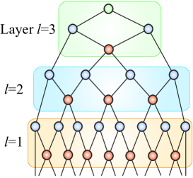
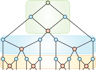
(c)

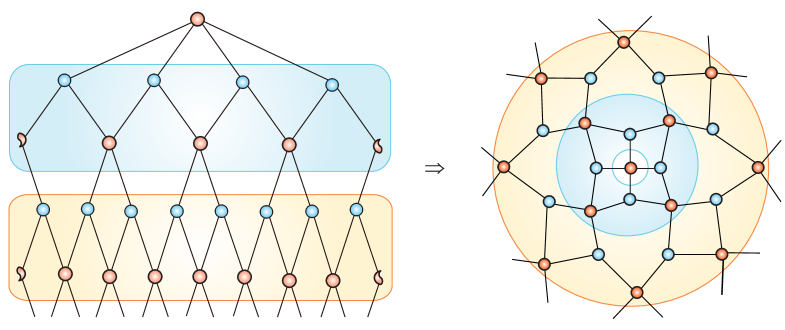
(d)

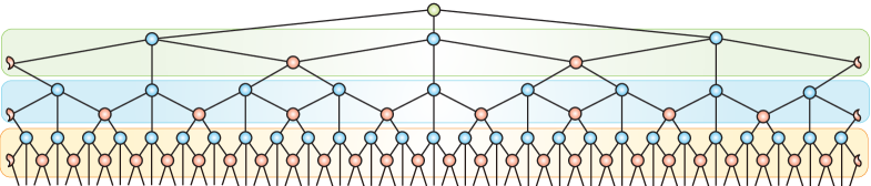
Figure 4.10: Various architectures of MERA tensor networks for the new generation of deep convolutional neural networks. (a) Basic binary MERA tensor network. The consecutive layers of disentangling and coarse-graining cores are indicated by different colors. For the network shown in (a) the number of cores after each such set of operations is approximately halved. (b) Improved (lower complexity) MERA network. (c) MERA with periodic boundary conditions. Red half-circles mean that they are connected, i.e., they build up one 4th-order core, as illustrated on the right panel of (c). (d) Ternary MERA (with the Periodic Boundary Conditions (PBC)) in which coarse grainers are also 4th-order tensors, i.e., three sites (modes) are coarse-grained into one effective site (mode).

For simplicity, this section focuses on 1D binary and ternary MERA architectures (see Figure 4.10(a) for basic binary MERA). Instead of writing complex mathematical formulas, it is more convenient to describe MERA tensor networks graphically, as illustrated in Figures 4.10(a), (b) and (c). Using the terminology from quantum physics, the standard binary MERA architecture contains three classes of core tensors: (i) disentanglers – 4th-order cores; (ii) isometries, also called the coarse-grainers, which are typically 3rd-order cores for binary MERA and 4th-order cores for ternary MERA; and (iii) one output core which is usually a matrix or a 4th-order core. Each MERA layer is constructed of a row of disentanglers and a row of coarse-grainers or isometries. Disentanglers remove the short-scale entanglement between the adjacent modes, while isometries renormalise each pair of modes to a single mode. Each renormalisation layer performs these operations on a scale of different length.

From the mapping perspective, the nodes (core tensors) can be considered as processing units, that is, the 4th-order cores map matrices to other matrices, while the coarse-grainers take matrices and map them to vectors. The key idea here is to realize that the “compression” capability arises from the hierarchy and the entanglement. As a matter of fact, the MERA network embodies the mutual information chain rule.

In other words, the main idea underlying MERA is that of disentangling the system at scales of various lengths, following coarse graining Renormalization Group (RG) flow in the system. The MERA is particularly effective for (scale invariant) critical points of physical systems. The key properties of MERA can be summarized, as follows [Evenbly and Vidal, 2015]:

• MERA can capture scale-invariance in input data;

• It reproduces a polynomial decay of correlations between inputs, in contrast to HT or TT networks which reproduce only exponential decay of correlations;

• MERA has the ability to compress tensor data much better than TT/HT tensor networks;

• It reproduces a logarithmic correction to the area law, therefore MERA is more powerful tensor network than HT/TTNS or TT/TC networks;

• MERA can be efficiently contracted due to unitary constraints imposed on core tensors.

Motivated by these features, we are currently investigating MERA tensor networks as powerful tools to model and analyze DCNNs. The main objective is to establish a precise connection between MERA tensor networks and extended models of DCNNs. This connection may provide exciting new insights about deep learning while also allowing for the construction of improved families of DCNNs, with potential application to more efficient data/image classification, clustering and prediction. In other words, we conjecture that the MERA and 2D TNs (see Figure 4.11) will lead to useful new results, potentially allowing not only for better characterization of expressive power of DCNNs, but also for new practical implementations. Conversely, the links and relations between TNs and DCNNs could lead to useful advances in the design of novel deep neural networks.

(a)                                             (b)

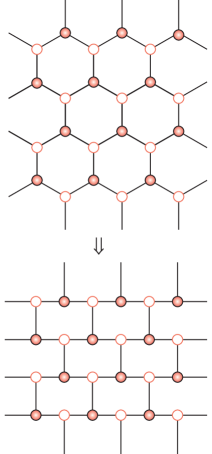
Figure 4.11: Architectures of 2D tensor networks as a potential model for DNNs. (a) A honey-comb lattice (top), which is equivalent to the brick-wall lattice (bottom), and (b) PEPS tensor networks with 5th-order (top) and up to 7th-order cores (bottom).

The MERA tensor networks, shown in Figure 4.10, may provide a much higher expressive power of deep learning in comparison to networks corresponding to HT/TT architectures, since this class of tensor networks can model more complex long-term correlations between input instances. This follows from the facts that for HT and TT tensor networks correlations between input variables decay exponentially, and the entanglement entropy saturates to a constant, while the more sophisticated MERA tensor networks provide polynomially decaying correlations.

We firmly believe that the insights into the theory of tensor networks and quantum many-body physics can provide better theoretical understanding of deep learning, together with the guidance for optimized DNNs design.

To summarize, the tensor network methodology and architectures discussed briefly in this section may be extended to allow analytic construction of new DCNNs. Moreover, systematic investigation of the correspondences between DNNs and a wide spectrum of TNs can provide a very fruitful perspective including verification of the existing conjectures and claims about operational similarities and correspondences between DNNs and TNs into a more rigorous and constructive framework.

Chapter 5 Discussion and Conclusions

Machine learning and data mining algorithms are becoming increasingly important in the analysis of large volume, multi-relational and multi-modal datasets, which are often conveniently represented as multiway arrays or tensors. The aim of this monograph has therefore been to provide the ML and data analytics communities with both a state-of-the-art review and new directions in tensor decompositions and tensor network approaches for fundamental problems of large-scale optimization. Our focus has been on supervised and unsupervised learning with tensors, tensor regression, support tensor machines, tensor canonical coloration analysis, higher-order and kernel partial least squares, and deep learning.

In order to demystify the concepts of tensor algebra and to provide a seamless transition from the flat view linear algebra to multi-view multilinear algebra, we have employed novel graphical representations of tensor networks to interpret mathematical expressions directly and intuitively on graphs rather than through tedious multiple-index relationships. Our main focus has been on the Tucker, Tensor Train (TT) and Hierarchical Tucker (HT) decompositions and their extensions or generalizations. To make the material self-contained, we have also addressed the important concept of tensorization and distributed representation of structured lower-order data in tensor network formats, as a tool to provide efficient higher-order representation of vectors, matrices and low-order tensors and the optimization of cost (loss) functions.

In order to combat the curse of dimensionality and possibly obtain a linear or even sub-linear complexity of storage and computational complexities, we have next addressed distributed representation of tensor functions through low-rank tensor networks. Finally, we have demonstrated how such approximations can be used to solve a wide class of huge-scale linear/multilinear dimensionality reduction and related optimization problems that are far from being tractable when using classical machine learning methods.

The lynchpin of this work are low-rank tensor network approximations and the associated tensor contraction algorithms, and we have elucidated how these can be used to convert otherwise intractable huge-scale optimization problems into a set of much smaller linked and/or distributed sub-problems of affordable sizes and complexity. In doing so, we have highlighted the ability of tensor networks to account for the couplings between the multiple variables, and for multimodal, incomplete and/or noisy data.

The Part 2 finishes with a discussion of the potential of tensor networks in the design of improved and optimized deep learning neural network architectures. It is our firm conviction that the links between tensor networks and deep learning provide both exciting new insights into multi-layer neural networks and a platform for the construction of improved families of DNNs, with potential applications in highly efficient data/image classifications, clustering and prediction.

Appendices

1 Estimation of Derivatives of GCF

The GCF of the observation and its derivatives are unknown, but can be estimated from the sample first GCF

$$\hat{\phi}_{{\bf x}}({\bf u})=\frac{1}{T}\sum_{t=1}^{T}\exp({\bf u}^{\text{T}}{\bf x}_{t})\,.$$ (A.1)

The $n$th-order partial derivatives of $\hat{\phi}_{{\bf x}}({\bf u})$ with respect to ${\bf u}$ are $n$th-order tensors of size $I\times I\times\cdots\times I$, given by

$$\mbox{\boldmath$\psi$}_{{\bf x}}^{(n)}({\bf u}) = \frac{\partial^{n}\hat{\phi}_{{\bf x}}({\bf u})}{\partial{\bf u}^{n}}=\frac{1}{T}\sum_{t=1}^{T}\exp({\bf u}^{\text{T}}{\bf x}_{t})\underbrace{({\bf x}_{t}\circ{\bf x}_{t}\circ\cdots\circ{\bf x}_{t})}_{\text{$n$ terms ${\bf x}_{t}$}}\,$$

$$= \mathop{\rm diag}\nolimits_{N}(\frac{1}{T}\exp({\bf u}^{\text{T}}{\bf x}_{t}))\times_{1}{\bf X}\times_{2}{\bf X}\cdots\times_{N}{\bf X}.$$

The order-$N$ derivatives of the second GCF are then given by

$$\underline{\mathbf{\Psi}}_{{\bf x}}({\bf u})=\sum_{k=1}^{N}\frac{(-1)^{k-1}\,(k-1)!}{\hat{\phi}_{{\bf x}}({\bf u})^{k}}\,\sum_{n_{1},n_{2},\ldots,n_{k}}m_{n_{1},n_{2},\ldots,n_{k}}\,{\mathcal{S}}(\mbox{\boldmath$\psi$}_{n_{1},n_{2},\ldots,n_{k}}({\bf u}))\,,\;$$

(A.2)

where $1\leq n_{1}\leq n_{2}\leq\cdots\leq n_{k}\leq N$, $n_{1}+n_{2}+\cdots+n_{k}=N$, $\mbox{\boldmath$\psi$}_{\{n_{1},n_{2},\ldots,n_{k}\}}({\bf u})$ are $N$th-order tensors constructed as an outer product of $k$ $n_{j}$th-order derivative tensors $\mbox{\boldmath$\psi$}_{{\bf x}}^{(n_{j})}({\bf u})$, that is

$$\mbox{\boldmath$\psi$}_{\{n_{1},n_{2},\ldots,n_{k}\}}({\bf u}) = \mbox{\boldmath$\psi$}_{{\bf x}}^{(n_{1})}({\bf u})\circ\mbox{\boldmath$\psi$}_{{\bf x}}^{(n_{2})}({\bf u})\circ\cdots\circ\mbox{\boldmath$\psi$}_{{\bf x}}^{(n_{k})}({\bf u}).$$ (A.3)

The operator ${\mathcal{S}}(\underline{\mathbf{A}})$ symmetrizes an $N$th-order tensor $\underline{\mathbf{A}}$, i.e., it yields a symmetric tensor, defined as

$${\mathcal{S}}(\underline{\mathbf{A}})=\frac{1}{N!}\sum_{\pi_{i}}\pi_{i}(\underline{\mathbf{A}})\,,$$ (A.4)

where $\pi_{i}$ runs through the list of all $N!$ possible tensor permutations of the $N$th-order tensor $\underline{\mathbf{A}}$. In the expression (A.2), this symmetrization can be simplified to operate only once on the resulting tensor $\underline{\mathbf{\Psi}}_{{\bf x}}({\bf u})$, instead on each tensor $\mbox{\boldmath$\psi$}_{n_{1},n_{2},\ldots,n_{k}}({\bf u})$.

The number $m_{n_{1},n_{2},\ldots,n_{k}}$ represents the total number of partitions of $\{1,2,\ldots,N\}$ into $k$ distinct parts, each having $n_{j}$ entries, $j=1,\ldots,k$. This number is given by

$$m_{n_{1},n_{2},\ldots,n_{k}}=\frac{N!}{\prod_{j=1}^{\bar{k}}(\bar{n}_{j}!)^{l_{j}}l_{j}!}\,,$$

where $\{1\leq{\bar{n}}_{1}<{\bar{n}}_{2}<\cdots<{\bar{n}}_{\bar{k}}\leq N\}$ denotes the set of distinct numbers of $\{n_{1},n_{2},\ldots,n_{k}\}$, while $1\leq l_{j}\leq N$ represents the replication number of $\bar{n}_{j}$ in $\{n_{1},n_{2},\ldots,n_{k}\}$, for $j=1,\ldots,\bar{k}$, i.e., $l_{1}{\bar{n}}_{1}+l_{2}{\bar{n}}_{2}+\cdots+l_{\bar{k}}{\bar{n}}_{\bar{k}}=N$.

The approximation of the derivative tensor $\underline{\mathbf{\Psi}}_{{\bf x}}({\bf u})$ for some low orders $N=2,3,\ldots,7$, are given below

$$\underline{\mathbf{\Psi}}_{{\bf x}}^{(2)}({\bf u}) =\frac{\mbox{\boldmath$\psi$}^{(2)}({\bf u})}{\hat{\phi}_{{\bf x}}({\bf u})}-\frac{\mbox{\boldmath$\psi$}^{(1)}({\bf u})\circ\mbox{\boldmath$\psi$}^{(1)}({\bf u})}{\hat{\phi}_{{\bf x}}^{2}({\bf u})}\,,$$

$$\underline{\mathbf{\Psi}}_{{\bf x}}^{(3)}({\bf u}) =\frac{\mbox{\boldmath$\psi$}^{(3)}{}({}{\bf u}{})}{\hat{\phi}_{{\bf x}}({\bf u})}-\frac{3{\mathcal{S}}(\mbox{\boldmath$\psi$}^{(1)}{}({}{\bf u}{})\circ\mbox{\boldmath$\psi$}^{(2)}{}({}{\bf u}{}))}{\hat{\phi}_{{\bf x}}^{2}({\bf u})}$$

$$\quad+2\,\frac{\mbox{\boldmath$\psi$}^{(1)}{}({\bf u})\circ\mbox{\boldmath$\psi$}^{(1)}{}({\bf u})\circ\mbox{\boldmath$\psi$}^{(1)}{}({\bf u})}{\hat{\phi}_{{\bf x}}^{3}({\bf u})}\,,$$

$$\underline{\mathbf{\Psi}}_{{\bf x}}^{(4)}({\bf u}) =\frac{\mbox{\boldmath$\psi$}^{(4)}({\bf u})}{\hat{\phi}_{{\bf x}}({\bf u})}-\frac{4\,{\mathcal{S}}(\mbox{\boldmath$\psi$}^{(1)}({\bf u})\circ\mbox{\boldmath$\psi$}^{(3)}({\bf u}))+3\,{\mathcal{S}}(\mbox{\boldmath$\psi$}^{(2)}({\bf u})\circ\mbox{\boldmath$\psi$}^{(2)}({\bf u}))}{\hat{\phi}_{{\bf x}}^{2}({\bf u})}$$

$$\quad+2\,\frac{6\,{\mathcal{S}}(\mbox{\boldmath$\psi$}^{(1)}({\bf u})\circ\mbox{\boldmath$\psi$}^{(1)}({\bf u})\circ\mbox{\boldmath$\psi$}^{(2)}({\bf u}))}{\hat{\phi}_{{\bf x}}^{3}({\bf u})}$$

$$\quad-6\,\frac{\mbox{\boldmath$\psi$}^{(1)}({\bf u})\circ\mbox{\boldmath$\psi$}^{(1)}({\bf u})\circ\mbox{\boldmath$\psi$}^{(1)}({\bf u})\circ\mbox{\boldmath$\psi$}^{(1)}({\bf u})}{\hat{\phi}_{{\bf x}}^{4}({\bf u})}\,,$$

$$\underline{\mathbf{\Psi}}_{{\bf x}}^{(5)}({\bf u}) ={\mathcal{S}}\left(\frac{\mbox{\boldmath$\psi$}^{(5)}({\bf u})}{\hat{\phi}_{{\bf x}}({\bf u})}-\frac{5\,\mbox{\boldmath$\psi$}_{1,4}({\bf u})+10\,\mbox{\boldmath$\psi$}_{2,3}({\bf u})}{\hat{\phi}_{{\bf x}}^{2}({\bf u})}\right.$$

$$\quad+2\,\frac{10\mbox{\boldmath$\psi$}_{1,1,3}({\bf u})+15\mbox{\boldmath$\psi$}_{1,2,2}({\bf u})}{\hat{\phi}_{{\bf x}}^{3}({\bf u})}-6\frac{15\mbox{\boldmath$\psi$}_{1,1,1,2}({\bf u})}{\hat{\phi}_{{\bf x}}^{4}({\bf u})}$$

$$\quad+\left.24\frac{\mbox{\boldmath$\psi$}_{1,1,1,1,1}({\bf u})}{\hat{\phi}_{{\bf x}}^{5}({\bf u})}\right)\,,$$

$$\underline{\mathbf{\Psi}}_{{\bf x}}^{(6)}({\bf u}) ={\mathcal{S}}\left(\frac{\mbox{\boldmath$\psi$}^{(6)}({\bf u})}{\hat{\phi}_{{\bf x}}({\bf u})}-\frac{6\,\mbox{\boldmath$\psi$}_{1,5}({\bf u})+15\,\mbox{\boldmath$\psi$}_{2,4}({\bf u})+10\,\mbox{\boldmath$\psi$}_{3,3}({\bf u})}{\hat{\phi}_{{\bf x}}^{2}({\bf u})}\right.$$

$$\quad+2\,\frac{15\,\mbox{\boldmath$\psi$}_{1,1,4}({\bf u})+60\,\mbox{\boldmath$\psi$}_{1,2,3}({\bf u})+15\,\mbox{\boldmath$\psi$}_{2,2,2}({\bf u})}{\hat{\phi}_{{\bf x}}^{3}({\bf u})}$$

$$\quad-6\,\frac{20\,\mbox{\boldmath$\psi$}_{1,1,1,3}({\bf u})+45\,\mbox{\boldmath$\psi$}_{1,1,2,2}({\bf u})}{\hat{\phi}_{{\bf x}}^{4}({\bf u})}$$

$$\quad+24\,\frac{15\,\mbox{\boldmath$\psi$}_{1,1,1,1,2}({\bf u})}{\hat{\phi}_{{\bf x}}^{5}({\bf u})}\left.-120\,\frac{\mbox{\boldmath$\psi$}_{1,1,1,1,1,1}}{\hat{\phi}_{{\bf x}}^{6}({\bf u})}\right)\,,$$

$$\underline{\mathbf{\Psi}}_{{\bf x}}^{(7)}({\bf u}) ={\mathcal{S}}\left(\frac{\mbox{\boldmath$\psi$}^{(7)}({\bf u})}{\hat{\phi}_{{\bf x}}({\bf u})}-\frac{7\,\mbox{\boldmath$\psi$}_{1,6}({\bf u})+21\,\mbox{\boldmath$\psi$}_{2,5}({\bf u})+35\,\mbox{\boldmath$\psi$}_{3,4}({\bf u})}{\hat{\phi}_{{\bf x}}^{2}({\bf u})}\right.$$

$$\quad+2\,\frac{21\,\mbox{\boldmath$\psi$}_{1,1,5}({\bf u})+105\,\mbox{\boldmath$\psi$}_{1,2,4}({\bf u})+70\,\mbox{\boldmath$\psi$}_{1,3,3}({\bf u})+105\,\mbox{\boldmath$\psi$}_{2,2,3}({\bf u})}{\hat{\phi}_{{\bf x}}^{3}({\bf u})}$$

$$\quad-6\,\frac{35\,\mbox{\boldmath$\psi$}_{1,1,1,4}({\bf u})+210\,\mbox{\boldmath$\psi$}_{1,1,2,3}({\bf u})+105\,\mbox{\boldmath$\psi$}_{1,2,2,2}({\bf u})}{\hat{\phi}_{{\bf x}}^{4}({\bf u})}$$

$$\quad+24\,\frac{35\,\mbox{\boldmath$\psi$}_{1,1,1,1,3}({\bf u})+105\,\mbox{\boldmath$\psi$}_{1,1,1,2,2}({\bf u})}{\hat{\phi}_{{\bf x}}^{5}({\bf u})}$$

$$\quad-120\,\frac{21\,\mbox{\boldmath$\psi$}_{1,1,1,1,1,2}({\bf u})}{\hat{\phi}_{{\bf x}}^{6}({\bf u})}\left.+720\,\frac{\mbox{\boldmath$\psi$}_{1,1,1,1,1,1,1}}{\hat{\phi}_{{\bf x}}^{7}({\bf u})}\right)\,.$$

The symmetrization in derivation of $\underline{\mathbf{\Psi}}_{{\bf x}}^{(4)}({\bf u})$ can be performed only once, as in the derivatives of orders-5, 6 and 7.

2 Higher Order Cumulants

When the mixtures are centered to have zero-mean, then the first derivative $\mbox{\boldmath$\psi$}_{{\bf x}}^{(1)}({\bf 0})=\frac{1}{T}\sum_{t}{\bf x}_{t}={\bf 0}$, which leads to $\mbox{\boldmath$\psi$}_{\{n_{1}=1,n_{2},\ldots,n_{k}\}}({\bf 0})$ being all zero for arbitrary partitions $\{n_{1}=1,n_{2},\ldots,n_{k}\}$. This simplifies the computation of the cumulant by ignoring the partitions $\{n_{1}=1,n_{2},\ldots,n_{k}\}$. For example, cumulants of order $2,3,\ldots,7$ can be computed as

$${\mathcal{K}}_{{\bf x}}^{(2)} =\mbox{\boldmath$\psi$}^{(2)}({\bf 0})=\frac{1}{T}\underline{\mathbf{I}}\times_{1}{\bf X}\times_{2}{\bf X}=\frac{1}{T}{\bf X}{\bf X}^{\text{T}}\,,$$

$${\mathcal{K}}_{{\bf x}}^{(3)} =\mbox{\boldmath$\psi$}^{(3)}({\bf 0})=\frac{1}{T}\underline{\mathbf{I}}\times_{1}{\bf X}\times_{2}{\bf X}\times_{3}{\bf X}\,,$$

$${\mathcal{K}}_{{\bf x}}^{(4)} =\mbox{\boldmath$\psi$}^{(4)}({\bf 0})-3{\mathcal{S}}(\mbox{\boldmath$\psi$}^{(2)}({\bf 0})\circ\mbox{\boldmath$\psi$}^{(2)}({\bf 0}))\,,$$

$${\mathcal{K}}_{{\bf x}}^{(5)} =\mbox{\boldmath$\psi$}^{(5)}({\bf 0})-10{\mathcal{S}}(\mbox{\boldmath$\psi$}^{(2)}({\bf 0})\circ\mbox{\boldmath$\psi$}^{(3)}({\bf 0}))\,,$$

$${\mathcal{K}}_{{\bf x}}^{(6)} ={\mathcal{S}}\left(\mbox{\boldmath$\psi$}^{(6)}({\bf 0})-15\mbox{\boldmath$\psi$}^{(2)}({\bf 0})\circ\mbox{\boldmath$\psi$}^{(4)}({\bf 0})-10\mbox{\boldmath$\psi$}^{(3)}({\bf 0})\circ\mbox{\boldmath$\psi$}^{(3)}({\bf 0})\right.$$

$$\quad\left.+30\mbox{\boldmath$\psi$}^{(2)}({\bf 0})\circ\mbox{\boldmath$\psi$}^{(2)}({\bf 0})\circ\mbox{\boldmath$\psi$}^{(2)}({\bf 0})\right)\,,$$

$${\mathcal{K}}_{{\bf x}}^{(7)} ={\mathcal{S}}\left(\mbox{\boldmath$\psi$}^{(7)}({\bf 0})-21\mbox{\boldmath$\psi$}^{(2)}({\bf 0})\circ\mbox{\boldmath$\psi$}^{(5)}({\bf 0})-35\mbox{\boldmath$\psi$}^{(3)}({\bf 0})\circ\mbox{\boldmath$\psi$}^{(4)}({\bf 0})\right.$$

$$\left.+210\mbox{\boldmath$\psi$}^{(2)}({\bf 0})\circ\mbox{\boldmath$\psi$}^{(2)}({\bf 0})\circ\mbox{\boldmath$\psi$}^{(3)}({\bf 0})\right)\,.$$

3 Elementary Core Tensor for the Convolution Tensor

The elementary core tensor $\underline{\mathbf{S}}$ of size $N\times\underbrace{2\times 2\times\cdots\times 2}_{\text{$(N+1)$ dimensions}}\times N$ is constructed from $2N$ $N$th-order sparse tensors $\underline{\mathbf{S}}_{1}$, $\underline{\mathbf{S}}_{2}$, …, $\underline{\mathbf{S}}_{2N}$ of size $2\times 2\times\cdots\times 2$, which take ones only at locations $(i_{1},i_{2},\ldots,i_{N})$ such that

$${\bar{i}}_{1}+{\bar{i}}_{2}+\cdots+{\bar{i}}_{N-1}+i_{N}=\begin{cases}\max(N-n+1,0)\quad&\text{odd}\;n,\\ \max(N-n+3,0)\quad&\text{even}\;n,\end{cases}$$ (A.5)

where $\bar{i}_{n}=2-i_{n}$.

The structure of the tensor $\underline{\mathbf{S}}$ based on $\underline{\mathbf{S}}_{n}$ is explained, as follows

$$\underline{\mathbf{S}}(1,:,\ldots,:,1,n)=\underline{\mathbf{S}}_{2n-1}\,,\quad\underline{\mathbf{S}}(1,:,\ldots,:,2,n)=\underline{\mathbf{S}}_{2n}\,,$$ (A.6)

for $n=1,\ldots,N$. The other sub-tensors $\underline{\mathbf{S}}(m,:,\ldots,:,n)$, $m=2,\ldots,N$, $n=1,\ldots,N$, are recursively defined as

$$\underline{\mathbf{S}}(m,:,\ldots,:,1,n) = \underline{\mathbf{S}}(m-1,:,\ldots,:,2,n),$$ (A.7)

$$\underline{\mathbf{S}}(m,:,\ldots,:,2,1) = \underline{\mathbf{S}}(m-1,:,\ldots,:,1,N),$$ (A.8)

$$\underline{\mathbf{S}}(m,:,\ldots,:,2,n) = \underline{\mathbf{S}}(m-1,:,\ldots,:,1,n-1).$$ (A.9)

According to definition of $\underline{\mathbf{S}}_{n}$, such tensors are orthogonal, i.e., their pair-wise inner products are zeros, and there are only $(N+1)$ such nonzero tensors, which are $\underline{\mathbf{S}}_{1}$, …, $\underline{\mathbf{S}}_{N}$ and $\underline{\mathbf{S}}_{N+2}$ for even $N$, and $\underline{\mathbf{S}}_{1}$, …, $\underline{\mathbf{S}}_{N}$ and $\underline{\mathbf{S}}_{N+1}$ for odd $N$; the remaining $(N-1)$ core tensors $\underline{\mathbf{S}}_{n}$ are zero tensors.

References

- Absil and Oseledets [2015] P.-A. Absil and I. V. Oseledets. Low-rank retractions: A survey and new results. Computational Optimization and Applications, 62(1):5–29, 2015. URL http://dx.doi.org/10.1007/s10589-014-9714-4.
- Absil et al. [2007] P.-A. Absil, C. G. Baker, and K. A. Gallivan. Trust-region methods on Riemannian manifolds. Foundations of Computational Mathematics, 7(3):303–330, 2007.
- Absil et al. [2008] P.-A. Absil, R. Mahony, and R. Sepulchre. Optimization Algorithms on Matrix Manifolds. Princeton University Press, 2008.
- Absil et al. [2013] P.-A. Absil, R. Mahony, and J. Trumpf. An extrinsic look at the Riemannian Hessian. In Geometric Science of Information, pages 361–368. Springer, 2013.
- Adler et al. [2002] R. L. Adler, J.-P. Dedieu, J. Y. Margulies, M. Martens, and M. Shub. Newton’s method on Riemannian manifolds and a geometric model for the human spine. IMA Journal of Numerical Analysis, 22(3):359–390, 2002.
- Allen and Maletic-Savatic [2011] G. I. Allen and M. Maletic-Savatic. Sparse non-negative generalized PCA with applications to metabolomics. Bioinformatics, 27 (21):3029–3035, 2011.
- Andersson and Bro [2000] C. A. Andersson and R. Bro. The N-way toolbox for MATLAB. Chemometrics and Intelligent Laboratory Systems, 52(1):1–4, 2000. URL http://www.models.life.ku.dk/source/nwaytoolbox/.
- Anselmi et al. [2015] F. Anselmi, L. Rosasco, C. Tan, and T. Poggio. Deep convolutional networks are hierarchical kernel machines. arXiv preprint arXiv:1508.01084, 2015.
- August et al. [2016] M. August, M. Bañuls, and T. Huckle. On the approximation of functionals of very large hermitian matrices represented as matrix product operators. CoRR, abs/1610.06086, 2016. URL http://arxiv.org/abs/1610.06086.
- Bach and Jordan [2005] F. R. Bach and M. I. Jordan. A probabilistic interpretation of canonical correlation analysis. Technical report, Department of Statistics, University of California, Berkeley, 2005.
- Bachmayr and Dahmen [2015] M. Bachmayr and W. Dahmen. Adaptive near-optimal rank tensor approximation for high-dimensional operator equations. Foundations of Computational Mathematics, 15(4):839–898, 2015.
- Bachmayr and Schneider [2016] M. Bachmayr and R. Schneider. Iterative methods based on soft thresholding of hierarchical tensors. Foundations of Computational Mathematics, pages 1–47, 2016.
- Bachmayr et al. [2016] M. Bachmayr, R. Schneider, and A. Uschmajew. Tensor networks and hierarchical tensors for the solution of high-dimensional partial differential equations. Foundations of Computational Mathematics, 16(6):1423–1472, 2016.
- Bader and Kolda [2006] B. W. Bader and T. G. Kolda. Algorithm 862: MATLAB tensor classes for fast algorithm prototyping. ACM Transactions on Mathematical Software, 32(4):635–653, 2006.
- Bader and Kolda [2015] B. W. Bader and T. G. Kolda. MATLAB tensor toolbox version 2.6, February 2015. URL http://csmr.ca.sandia.gov/~tgkolda/TensorToolbox/.
- Ballani and Grasedyck [2013] J. Ballani and L. Grasedyck. A projection method to solve linear systems in tensor format. Numerical Linear Algebra with Applications, 20(1):27–43, 2013.
- Batselier et al. [2016a] K. Batselier, Z. Chen, H. Liu, and N. Wong. A tensor-based volterra series black-box nonlinear system identification and simulation framework. In 2016 IEEE/ACM International Conference on Computer-Aided Design (ICCAD), pages 1–7, 2016a.
- Batselier et al. [2016b] K. Batselier, Z. Chen, and N. Wong. Tensor train alternating linear scheme for MIMO Volterra system identification. CoRR, abs/1607.00127, 2016b. URL http://arxiv.org/abs/1607.00127.
- Benner et al. [2016] P. Benner, V. Khoromskaia, and B. N. Khoromskij. A reduced basis approach for calculation of the Bethe–Salpeter excitation energies by using low-rank tensor factorisations. Molecular Physics, 114(7-8):1148–1161, 2016.
- Benson et al. [2015] A. R. Benson, D. F. Gleich, and J. Leskovec. Tensor spectral clustering for partitioning higher-order network structures. In Proceedings of the 2015 SIAM International Conference on Data Mining, pages 118–126, 2015.
- Bento et al. [2016] G. C. Bento, O. P. Ferreira, and J. G. Melo. Iteration-complexity of gradient, subgradient and proximal point methods on Riemannian manifolds. arXiv preprint arXiv:1609.04869, 2016.
- Beylkin and Mohlenkamp [2005] G. Beylkin and M. J. Mohlenkamp. Algorithms for numerical analysis in high dimensions. SIAM Journal on Scientific Computing, 26(6):2133–2159, 2005.
- Biamonte et al. [2016] J. Biamonte, P. Wittek, N. Pancotti, P. Rebentrost, N. Wiebe, and S. Lloyd. Quantum machine learning. arXiv preprint arXiv:1611.09347, 2016.
- Billaud-Friess et al. [2014] M. Billaud-Friess, A. Nouy, and O. Zahm. A tensor approximation method based on ideal minimal residual formulations for the solution of high-dimensional problems. ESAIM: Mathematical Modelling and Numerical Analysis, 48(6):1777–1806, 2014.
- Billings [2013] S. A. Billings. Nonlinear System Identification: NARMAX Methods in the Time, Frequency, and Spatio-Temporal Domains. John Wiley & Sons, 2013.
- Bini [1995] D. Bini. Toeplitz matrices, algorithms and applications. ECRIM News Online Edition,, 3(22):852–872, 1995.
- Biswas and Milanfar [2016] S. K. Biswas and P. Milanfar. Linear support tensor machine: Pedestrian detection in thermal infrared images. arXiv preprint arXiv:1609.07878, 2016.
- Blumensath and Davies [2009] T. Blumensath and M. E. Davies. Iterative hard thresholding for compressed sensing. Applied and Computational Harmonic Analysis, 27(3):265–274, 2009.
- Bolten et al. [2016] M. Bolten, K. Kahl, and S. Sokolović. Multigrid Methods for Tensor Structured Markov Chains with Low Rank Approximation. SIAM Journal on Scientific Computing, 38(2):A649–A667, 2016. URL http://adsabs.harvard.edu/abs/2016arXiv160506246B.
- Bonnabel [2013] S. Bonnabel. Stochastic gradient descent on Riemannian manifolds. IEEE Transactions on Automatic Control, 58(9):2217–2229, 2013.
- Boumal and Absil [2011] N. Boumal and P.-A. Absil. RTRMC: A Riemannian trust-region method for low-rank matrix completion. In J. Shawe-Taylor, R. S. Zemel, P. Bartlett, F. C. N. Pereira, and K. Q. Weinberger, editors, Advances in Neural Information Processing Systems 24 (NIPS), pages 406–414. MIT, 2011.
- Boumal et al. [2014] N. Boumal, B. Mishra, P.-A. Absil, and R. Sepulchre. Manopt, a MATLAB toolbox for optimization on manifolds. Journal of Machine Learning Research, 15(1):1455–1459, 2014.
- Boussé et al. [2015] M. Boussé, O. Debals, and L. De Lathauwer. A tensor-based method for large-scale blind source separation using segmentation. Technical Report Tech. Report 15-59, ESAT-STADIUS, KU Leuven, Leuven, Belgium, 2015, submitted.
- Boyd et al. [2011] S. Boyd, N. Parikh, E. Chu, B. Peleato, and J. Eckstein. Distributed optimization and statistical learning via the alternating direction method of multipliers. Foundations and Trends® in Machine Learning, 3(1):1–122, 2011.
- Bro [1996] R. Bro. Multiway calibration. Multilinear PLS. Journal of Chemometrics, 10(1):47–61, 1996.
- Bursill et al. [1996] R. J. Bursill, T. Xiang, and G. A. Gehring. The density matrix renormalization group for a quantum spin chain at non-zero temperature. Journal of Physics: Condensed Matter, 8(40):L583, 1996.
- Caiafa and Cichocki [2013] C. Caiafa and A. Cichocki. Computing sparse representations of multidimensional signals using Kronecker bases. Neural Computaion, 25(1):186–220, 2013.
- Caiafa and Cichocki [2015] C. Caiafa and A. Cichocki. Stable, robust, and super–fast reconstruction of tensors using multi-way projections. IEEE Transactions on Signal Processing, 63(3):780–793, 2015.
- Calabrese and Cardy [2004] P. Calabrese and J. Cardy. Entanglement entropy and quantum field theory. Journal of Statistical Mechanics: Theory and Experiment, 2004(06):P06002, 2004.
- Cambier and Absil [2016] L. Cambier and P.-A. Absil. Robust low-rank matrix completion by Riemannian optimization. SIAM Journal on Scientific Computing, 38(5):S440–S460, 2016.
- Candes et al. [2008] E. J. Candes, M. B. Wakin, and S. P. Boyd. Enhancing sparsity by reweighted minimization. Journal of Fourier Analysis and Applications, 14(5-6):877–905, 2008.
- Chan et al. [2004] A. B. Chan, N. Vasconcelos, and P. J. Moreno. A family of probabilistic kernels based on information divergence. Technical report, University of California, San Diego, CA, SVCL-TR-2004-1, 2004.
- Chatterjee and Yu [2016] R. Chatterjee and T. Yu. Generalized coherent states, reproducing kernels, and quantum support vector machines. arXiv preprint arXiv:1612.03713, 2016.
- Chen et al. [2014] C. Chen, J. Huang, L. He, and H. Li. Preconditioning for accelerated iteratively reweighted least squares in structured sparsity reconstruction. In The IEEE Conference on Computer Vision and Pattern Recognition (CVPR), June 2014.
- Chen [2016] H. Chen. Structured Tensors: Theory and Applications. PhD thesis, The Hong Kong Polytechnic University, Hong Kong, 2016.
- Chen et al. [2017] J. Chen, S. Cheng, H. Xie, L. Wang, and T. Xiang. On the equivalence of Restricted Boltzmann Machines and Tensor Network States. ArXiv e-prints, 2017.
- Chen and Billings [1989] S. Chen and S. A. Billings. Representations of non-linear systems: the narmax model. International Journal of Control, 49(3):1013–1032, 1989. URL http://www.tandfonline.com/doi/abs/10.1080/00207178908559683.
- Chen et al. [2016] Z. Chen, K. Batselier, J. A. K. Suykens, and N. Wong. Parallelized tensor train learning of polynomial classifiers. CoRR, abs/1612.06505, 2016. URL http://arxiv.org/abs/1612.06505.
- Cho et al. [2016] H. Cho, D. Venturi, and G. E. Karniadakis. Numerical methods for high-dimensional probability density function equations. Journal of Computational Physics, 305:817–837, 2016.
- Choi and Vishwanathan [2014] J. H. Choi and S. Vishwanathan. DFacTo: Distributed factorization of tensors. In Advances in Neural Information Processing Systems, pages 1296–1304, 2014.
- Chu et al. [2013] D. Chu, L.-Z. Liao, M. K. Ng, and X. Zhang. Sparse canonical correlation analysis: New formulation and algorithm. IEEE Transactions on Pattern Analysis and Machine Intelligence, 35(12):3050–3065, 2013.
- Cichocki [2011] A. Cichocki. Tensor decompositions: New concepts in brain data analysis? Journal of the Society of Instrument and Control Engineers, 50(7):507–516, 2011.
- Cichocki [2013] A. Cichocki. Era of big data processing: A new approach via tensor networks and tensor decompositions, (invited). In Proceedings of the International Workshop on Smart Info-Media Systems in Asia (SISA2013), September 2013. URL http://arxiv.org/abs/1403.2048.
- Cichocki [2014] A. Cichocki. Tensor networks for big data analytics and large-scale optimization problems. arXiv preprint arXiv:1407.3124, 2014.
- Cichocki and Zdunek [2006] A. Cichocki and R. Zdunek. Multilayer nonnegative matrix factorisation. Electronics Letters, 42(16):1, 2006.
- Cichocki and Zdunek [2007] A. Cichocki and R. Zdunek. Regularized alternating least squares algorithms for non-negative matrix/tensor factorization. In International Symposium on Neural Networks, pages 793–802. Springer, 2007.
- Cichocki et al. [1995] A. Cichocki, W. Kasprzak, and S. Amari. Multi-layer neural networks with a local adaptive learning rule for blind separation of source signals. In Proc. Int. Symposium Nonlinear Theory and Applications (NOLTA), Las Vegas, NV, pages 61–65. Citeseer, 1995.
- Cichocki et al. [2009] A. Cichocki, R. Zdunek, A.-H. Phan, and S. Amari. Nonnegative Matrix and Tensor Factorizations: Applications to Exploratory Multi-way Data Analysis and Blind Source Separation. Wiley, Chichester, 2009.
- Cichocki et al. [2011] A. Cichocki, S. Cruces, and S. Amari. Generalized alpha-beta divergences and their application to rubust nonnegative matrix factorization. Entropy, 13:134–170, 2011.
- Cichocki et al. [2015] A. Cichocki, S. Cruces, and S. Amari. Log-determinant divergences revisited: Alpha-beta and gamma log-det divergences. Entropy, 17(5):2988–3034, 2015.
- Cichocki et al. [2016] A. Cichocki, N. Lee, I. Oseledets, A.-H. Phan, Q. Zhao, and D. P. Mandic. Tensor Networks for Dimensionality Reduction and Large-scale Optimization: Part 1 Low-Rank Tensor Decompositions. Foundations and Trends® in Machine Learning, 9(4-5):249–429, 2016.
- Cohen and Shashua [2016] N. Cohen and A. Shashua. Inductive bias of deep convolutional networks through pooling geometry. CoRR, abs/1605.06743, 2016. URL http://arxiv.org/abs/1605.06743.
- Cohen and Shashua [2016] N. Cohen and A. Shashua. Convolutional rectifier networks as generalized tensor decompositions. In Proceedings of The 33rd International Conference on Machine Learning, pages 955–963, 2016.
- Cohen et al. [2016] N. Cohen, O. Sharir, and A. Shashua. On the expressive power of deep learning: A tensor analysis. In 29th Annual Conference on Learning Theory, pages 698–728, 2016.
- Comon and Rajih [2006] P. Comon and M. Rajih. Blind identification of under-determined mixtures based on the characteristic function. Signal Processing, 86(9):2271–2281, 2006.
- Corona et al. [2015] E. Corona, A. Rahimian, and D. Zorin. A Tensor-Train accelerated solver for integral equations in complex geometries. arXiv preprint arXiv:1511.06029, November 2015.
- Cortes and Vapnik [1995] C. Cortes and V. Vapnik. Support-vector networks. Machine Learning, 20(3):273–297, 1995.
- Cunningham and Ghahramani [2015] J. P. Cunningham and Z. Ghahramani. Linear dimensionality reduction: Survey, insights, and generalizations. Journal of Machine Learning Research, 16:2859–2900, 2015.
- Da Silva and Herrmann [2013] C. Da Silva and F. J. Herrmann. Hierarchical Tucker tensor optimization – Applications to tensor completion. In Proc. 10th International Conference on Sampling Theory and Applications, volume 1, 2013.
- d’Aspremont et al. [2007] A. d’Aspremont, L. El Ghaoui, M. I. Jordan, and G. Lanckriet. A direct formulation for sparse PCA using semidefinite programming. SIAM Review, 49(3):434–448, 2007.
- Debals and De Lathauwer [2015] O. Debals and L. De Lathauwer. Stochastic and deterministic tensorization for blind signal separation. In E. Vincent, A. Yeredor, Z. Koldovsky, and P. Tichavský, editors, Proceedings of the 12th International Conference Latent Variable Analysis and Signal Separation, pages 3–13. Springer International Publishing, 2015.
- Debals et al. [2016a] O. Debals, M. Van Barel, and L. De Lathauwer. Löwner-based blind signal separation of rational functions with applications. IEEE Transactions on Signal Processing, 64(8):1909–1918, 2016a.
- Debals et al. [2016b] O. Debals, M. Sohail, and L. De Lathauwer. Analytical multi-modulus algorithms based on coupled canonical polyadic decompositions. Technical report, ESAT-STADIUS, KU Leuven, Leuven, Belgium, 2016b.
- Dolgov [2013] S. V. Dolgov. TT-GMRES: Solution to a linear system in the structured tensor format. Russian Journal of Numerical Analysis and Mathematical Modelling, 28(2):149–172, 2013.
- Dolgov [2014] S. V. Dolgov. Tensor Product Methods in Numerical Simulation of High-dimensional Dynamical Problems. PhD thesis, Faculty of Mathematics and Informatics, University Leipzig, Germany, Leipzig, Germany, 2014.
- Dolgov and Khoromskij [2013] S. V. Dolgov and B. N. Khoromskij. Two-level QTT-Tucker format for optimized tensor calculus. SIAM Journal on Matrix Analysis and Applications, 34(2):593–623, 2013.
- Dolgov and Khoromskij [2015] S. V. Dolgov and B. N. Khoromskij. Simultaneous state-time approximation of the chemical master equation using tensor product formats. Numerical Linear Algebra with Applications, 22(2):197–219, 2015.
- Dolgov and Savostyanov [2013a] S. V. Dolgov and D. V. Savostyanov. Alternating minimal energy methods for linear systems in higher dimensions. Part I: SPD systems. arXiv preprint arXiv:1301.6068, 2013a.
- Dolgov and Savostyanov [2013b] S. V. Dolgov and D. V. Savostyanov. Alternating minimal energy methods for linear systems in higher dimensions. Part II: Faster algorithm and application to nonsymmetric systems. arXiv preprint arXiv:1304.1222, 2013b.
- Dolgov and Savostyanov [2014] S. V. Dolgov and D. V. Savostyanov. Alternating minimal energy methods for linear systems in higher dimensions. SIAM Journal on Scientific Computing, 36(5):A2248–A2271, 2014.
- Dolgov et al. [2014] S. V. Dolgov, B. N. Khoromskij, I. V. Oseledets, and D. V. Savostyanov. Computation of extreme eigenvalues in higher dimensions using block tensor train format. Computer Physics Communications, 185(4):1207–1216, 2014.
- Dolgov et al. [2016] S. V. Dolgov, J. W. Pearson, D. V. Savostyanov, and M. Stoll. Fast tensor product solvers for optimization problems with fractional differential equations as constraints. Applied Mathematics and Computation, 273:604–623, 2016.
- Eisert et al. [2010] J. Eisert, M. Cramer, and M. B. Plenio. Colloquium: Area laws for the entanglement entropy. Reviews of Modern Physics, 82(1):277, 2010.
- El Alaoui et al. [2016] A. El Alaoui, X. Cheng, A. Ramdas, M. J. Wainwright, and M. I. Jordan. Asymptotic behavior of -based Laplacian regularization in semi-supervised learning. arXiv e-prints arXiv:1603.00564, March 2016.
- Endres and Schindelin [2003] D. M. Endres and J. E. Schindelin. A new metric for probability distributions. IEEE Transactions on Information Theory, 49(7):1858–1860, 2003.
- Espig et al. [2012] M. Espig, M. Schuster, A. Killaitis, N. Waldren, P. Wähnert, S. Handschuh, and H. Auer. TensorCalculus library, 2012. URL http://gitorious.org/tensorcalculus.
- Evenbly and Vidal [2009] G. Evenbly and G. Vidal. Algorithms for entanglement renormalization. Physical Review B, 79(14):144108, 2009.
- Evenbly and Vidal [2015] G. Evenbly and G. Vidal. Tensor network renormalization yields the multiscale entanglement renormalization Ansatz. Physical Review Letters, 115(20):200401, 2015.
- Evenbly and White [2016a] G. Evenbly and S. R. White. Entanglement renormalization and wavelets. Physical Review Letters, 116(14):140403, 2016a.
- Evenbly and White [2016b] G. Evenbly and S. R. White. Representation and design of wavelets using unitary circuits. arXiv e-prints, 2016b.
- Favier et al. [2012] G. Favier, A. Y. Kibangou, and T. Bouilloc. Nonlinear system modeling and identification using Volterra-PARAFAC models. International Journal of Adaptive Control and Signal Processing, 26(1), 2012. URL http://dx.doi.org/10.1002/acs.1272.
- Fischer and Igel [2012] A. Fischer and C. Igel. An introduction to restricted Boltzmann machines. In Iberoamerican Congress on Pattern Recognition, pages 14–36. Springer, 2012.
- Foucart and Rauhut [2013] S. Foucart and H. Rauhut. A Mathematical Introduction to Compressive Sensing. Springer, New York, 2013.
- Friedman et al. [2008] J. Friedman, T. Hastie, and R. Tibshirani. Sparse inverse covariance estimation with the graphical Lasso. Biostatistics, 9(3):432–441, 2008.
- Gao and Wu [2012] C. Gao and X.-J. Wu. Kernel support tensor regression. Procedia Engineering, 29:3986–3990, 2012.
- Garipov et al. [2016] T. Garipov, D. Podoprikhin, A. Novikov, and D. P. Vetrov. Ultimate tensorization: compressing convolutional and FC layers alike. CoRR, abs/1611.03214, 2016.
- Garreis and Ulbrich [2017] S. Garreis and M. Ulbrich. Constrained optimization with low-rank tensors and applications to parametric problems with PDEs. SIAM Journal on Scientific Computing, 39(1):A25–A54, 2017.
- Gleich et al. [2015] D. F. Gleich, L.-H. Lim, and Y. Yu. Multilinear PageRank. SIAM Journal on Matrix Analysis and Applications, 36(4):1507–1541, 2015.
- Goodfellow et al. [2016] I. Goodfellow, Y. Bengio, and A. Courville. Deep Learning. MIT Press, 2016, Cambridge, MA. http://www.deeplearningbook.org.
- Grasedyck [2010] L. Grasedyck. Hierarchical singular value decomposition of tensors. SIAM Journal on Matrix Analysis and Applications, 31(4):2029–2054, 2010.
- Grasedyck et al. [2013] L. Grasedyck, D. Kessner, and C. Tobler. A literature survey of low-rank tensor approximation techniques. GAMM-Mitteilungen, 36:53–78, 2013.
- Grasedyck et al. [2015] L. Grasedyck, M. Kluge, and S. Krämer. Variants of alternating least squares tensor completion in the tensor train format. SIAM Journal on Scientific Computing, 37(5):A2424–A2450, 2015.
- Gray [2006] R. M. Gray. Toeplitz and circulant matrices: A review. Foundations and Trends® in Communications and Information Theory, 2(3):155–239, 2006.
- Gross et al. [2010] D. Gross, Y.-K. Liu, S. T. Flammia, S. Becker, and J. Eisert. Quantum state tomography via compressed sensing. Phys. Rev. Lett., 105:150401, 2010. URL http://link.aps.org/doi/10.1103/PhysRevLett.105.150401.
- Hao et al. [2013] Z. Hao, L. He, B. Chen, and X. Yang. A linear support higher-order tensor machine for classification. IEEE Transactions on Image Processing, 22(7):2911–2920, 2013.
- Hoff [2015] P. D. Hoff. Multilinear tensor regression for longitudinal relational data. The Annals of Applied Statistics, 9(3):1169–1193, 2015.
- Holtz et al. [2012a] S. Holtz, T. Rohwedder, and R. Schneider. The alternating linear scheme for tensor optimization in the tensor train format. SIAM Journal on Scientific Computing, 34(2), 2012a.
- Holtz et al. [2012b] S. Holtz, T. Rohwedder, and R. Schneider. On manifolds of tensors of fixed TT-rank. Numerische Mathematik, 120(4):701–731, 2012b.
- Hosseini and Sra [2015] R. Hosseini and S. Sra. Matrix manifold optimization for Gaussian mixtures. In Advances in Neural Information Processing Systems, pages 910–918, 2015.
- Hou [2017] M. Hou. Tensor-based Regression Models and Applications. PhD thesis, University Laval, Quebec, Canada, 2017.
- Hou et al. [2015] M. Hou, Y. Wang, and B. Chaib-draa. Online local Gaussian processes for tensor-variate regression: Application to fast reconstruction of limb movements from brain signal. In Proceedings of the 2015 IEEE International Conference on Acoustics, Speech and Signal Processing (ICASSP), pages 5490–5494. IEEE, 2015.
- Hou et al. [2016b] M. Hou, Q. Zhao, B. Chaib-draa, and A. Cichocki. Common and discriminative subspace kernel-based multiblock tensor partial least squares regression. In Proc. of Thirtieth AAAI Conference on Artificial Intelligence, 2016a.
- Huang et al. [2009] J. Z. Huang, H. Shen, and A. Buja. The analysis of two-way functional data using two-way regularized singular value decompositions. Journal of the American Statistical Association, 104(488):1609–1620, 2009. URL http://EconPapers.repec.org/RePEc:bes:jnlasa:v:104:i:488:y:2009:p:1609-1620.
- Huang et al. [2016] R.-Z. Huang, H.-J. Liao, Z.-Y. Liu, H.-D. Xie, Z.-Y. Xie, H.-H. Zhao, J. Chen, and T. Xiang. A generalized Lanczos method for systematic optimization of tensor network states. ArXiv e-prints, 2016.
- Hubig et al. [2015] C. Hubig, I. P. McCulloch, U. Schollwöck, and F. A. Wolf. Strictly single-site DMRG algorithm with subspace expansion. Physical Review B, 91(15):155115, 2015.
- Hubig et al. [2017] C. Hubig, I. P. McCulloch, and U. Schollwöck. Generic construction of efficient matrix product operators. Phys. Rev. B, 95:035129, 2017. URL http://link.aps.org/doi/10.1103/PhysRevB.95.035129.
- Huckle and Waldherr [2012] T. Huckle and K. Waldherr. Subspace iteration methods in terms of matrix product states. PAMM, 12(1):641–642, 2012.
- Imaizumi and Hayashi [2016] M. Imaizumi and K. Hayashi. Doubly decomposing nonparametric tensor regression. In Proceedings of the 33rd International Conference on Machine Learning, pages 727–736, 2016.
- Inoue et al. [2009] K. Inoue, K. Hara, and K. Urahama. Robust multilinear principal component analysis. In IEEE 12th International Conference on Computer Vision, pages 591–597. IEEE, 2009.
- Ishteva et al. [2009] M. Ishteva, L. De Lathauwer, P. A. Absil, and S. Van Huffel. Differential-geometric Newton method for the best rank-(r, r, r) approximation of tensors. Numerical Algorithms, 51(2):179–194, 2009.
- Ishteva et al. [2011] M. Ishteva, P. A. Absil, S. Van Huffel, and L. De Lathauwer. Best low multilinear rank approximation of higher-order tensors, based on the Riemannian trust-region scheme. SIAM Journal on Matrix Analysis and Applications, 32(1):115–135, 2011.
- Jeon et al. [2015] I. Jeon, E. Papalexakis, U. Kang, and C. Faloutsos. Haten2: Billion-scale tensor decompositions. In Proceedings of the 31st IEEE International Conference on Data Engineering (ICDE), pages 1047–1058. IEEE, 2015.
- Jeon et al. [2016] I. Jeon, E. E. Papalexakis, C. Faloutsos, L. Sael, and U. Kang. Mining billion-scale tensors: Algorithms and discoveries. The VLDB Journal, pages 1–26, 2016.
- Jolliffe [1982] I. Jolliffe. A note on the use of principal components in regression. Applied Statistics, pages 300–303, 1982.
- Kamal et al. [2016] M. H. Kamal, B. Heshmat, R. Raskar, P. Vandergheynst, and G. Wetzstein. Tensor low-rank and sparse light field photography. Computer Vision and Image Understanding, 145:172–181, 2016.
- Kang et al. [2012] U. Kang, E. E. Papalexakis, A. Harpale, and C. Faloutsos. GigaTensor: Scaling tensor analysis up by 100 times – algorithms and discoveries. In Proceedings of the 18th ACM SIGKDD International Conference on Knowledge Discovery and Data Mining (KDD ’12), pages 316–324, August 2012.
- Kao et al. [2015] Y.-J. Kao, Y.-D. Hsieh, and P. Chen. Uni10: An open-source library for tensor network algorithms. In Journal of Physics: Conference Series, volume 640, page 012040. IOP Publishing, 2015.
- Karlsson et al. [2016] L. Karlsson, D. Kressner, and A. Uschmajew. Parallel algorithms for tensor completion in the CP format. Parallel Computing, 57:222–234, 2016.
- Kasai and Mishra [2015] H. Kasai and B. Mishra. Riemannian preconditioning for tensor completion. arXiv preprint arXiv:1506.02159, 2015.
- Kazeev et al. [2013] V. A. Kazeev, B. N. Khoromskij, and E. E. Tyrtyshnikov. Multilevel Toeplitz matrices generated by tensor-structured vectors and convolution with logarithmic complexity. SIAM Journal on Scientific Computing, 35(3), 2013.
- Khoromskaia and Khoromskij [2016] V. Khoromskaia and B. N. Khoromskij. Fast tensor method for summation of long-range potentials on 3D lattices with defects. Numerical Linear Algebra with Applications, 23(2):249–271, 2016. URL http://dx.doi.org/10.1002/nla.2023.
- Khoromskij [2011a] B. N. Khoromskij. -quantics approximation of - tensors in high-dimensional numerical modeling. Constructive Approximation, 34(2):257–280, 2011a.
- Khoromskij [2011b] B. N. Khoromskij. Tensors-structured numerical methods in scientific computing: Survey on recent advances. Chemometrics and Intelligent Laboratory Systems, 110(1):1–19, 2011b. URL http://www.mis.mpg.de/de/publications/preprints/2010/prepr2010-21.html.
- Khoromskij and Miao [2014] B. N. Khoromskij and S. Miao. Superfast wavelet transform using quantics-TT approximation. I. application to Haar wavelets. Computational Methods in Applied Mathematics, 14(4):537–553, 2014. URL http://dx.doi.org/10.1515/cmam-2014-0016.
- Khoromskij and Oseledets [2010] B. N. Khoromskij and I. Oseledets. Quantics-TT collocation approximation of parameter-dependent and stochastic elliptic PDEs. Computational Methods in Applied Mathematics, 10(4):376–394, 2010.
- Khoromskij and Schwab [2011] B. N. Khoromskij and C. Schwab. Tensor-structured Galerkin approximation of parametric and stochastic elliptic PDEs. SIAM Journal on Scientific Computing, 33(1):364–385, 2011.
- Khoromskij and Veit [2016] B. N. Khoromskij and A. Veit. Efficient computation of highly oscillatory integrals by using QTT tensor approximation. Computational Methods in Applied Mathematics, 16(1):145–159, 2016.
- Khrulkov and Oseledets [2016] V. Khrulkov and I. Oseledets. Desingularization of bounded-rank matrix sets. arXiv preprint arXiv:1612.03973, 2016.
- Kim et al. [2015] H.-J. Kim, E. Ollila, and V. Koivunen. New robust Lasso method based on ranks. In 23rd European Signal Processing Conference (EUSIPCO), pages 699–703. IEEE, 2015.
- Kim and Cipolla [2009] T. K. Kim and R. Cipolla. Canonical correlation analysis of video volume tensors for action categorization and detection. IEEE Transactions on Pattern Analysis and Machine Intelligence, 31(8):1415–1428, 2009.
- Kim et al. [2007] T. K. Kim, S. F. Wong, and R. Cipolla. Tensor canonical correlation analysis for action classification. In Proceedings of the IEEE Conference on Computer Vision and Pattern Recognition (CVPR’07), pages 1–8, 2007.
- Koch and Lubich [2007] O. Koch and C. Lubich. Dynamical low rank approximation. SIAM Journal on Matrix Analysis and Applications, 29:434–454, 2007.
- Koch and Lubich [2010] O. Koch and C. Lubich. Dynamical tensor approximation. SIAM Journal on Matrix Analysis and Applications, 31(5):2360–2375, 2010.
- Koep and Weichwald [2016] N. Koep and S. Weichwald. Pymanopt: A Python Toolbox for manifold optimization using automatic differentiation. arXiv preprint arXiv:1603.03236, 2016.
- Kokiopoulou et al. [2011] E. Kokiopoulou, J. Chen, and Y. Saad. Trace optimization and eigenproblems in dimension reduction methods. Numerical Linear Algebra with Applications, 18(3):565–602, 2011.
- Kolesnikov and Oseledets [2016] D. Kolesnikov and I. V. Oseledets. Convergence analysis of projected fixed-point iteration on a low-rank matrix manifold. arXiv preprint arXiv:1604.02111, 2016.
- Kotsia et al. [2012] I. Kotsia, W. Guo, and I. Patras. Higher rank support tensor machines for visual recognition. Pattern Recognition, 45(12):4192–4203, 2012.
- Kressner and Macedo [2014] D. Kressner and F. Macedo. Low-rank tensor methods for communicating Markov processes. In Quantitative Evaluation of Systems, pages 25–40. Springer, 2014.
- Kressner and Tobler [2011a] D. Kressner and C. Tobler. Low-rank tensor Krylov subspace methods for parametrized linear systems. SIAM Journal on Matrix Analysis and Applications, 32(4):1288–1316, 2011a.
- Kressner and Tobler [2011b] D. Kressner and C. Tobler. Preconditioned low-rank methods for high-dimensional elliptic PDE eigenvalue problems. Computational Methods in Applied Mathematics, 11(3):363–381, 2011b.
- Kressner and Tobler [2014] D. Kressner and C. Tobler. Algorithm 941: HTucker–A MATLAB toolbox for tensors in hierarchical Tucker format. ACM Transactions on Mathematical Software, 40(3):22, 2014.
- Kressner and Uschmajew [2016] D. Kressner and A. Uschmajew. On low-rank approximability of solutions to high-dimensional operator equations and eigenvalue problems. Linear Algebra and its Applications, 493:556–572, 2016.
- Kressner et al. [2014a] D. Kressner, M. Steinlechner, and A. Uschmajew. Low-rank tensor methods with subspace correction for symmetric eigenvalue problems. SIAM Journal on Scientific Computing, 36(5):A2346–A2368, 2014a.
- Kressner et al. [2014b] D. Kressner, M. Steinlechner, and B. Vandereycken. Low-rank tensor completion by Riemannian optimization. BIT Numerical Mathematics, 54(2):447–468, 2014b.
- Kressner et al. [2016] D. Kressner, M. Steinlechner, and B. Vandereycken. Preconditioned low-rank Riemannian optimization for linear systems with tensor product structure. SIAM Journal on Scientific Computing, 38(4):A2018–A2044, 2016.
- Kumar et al. [2009] R. Kumar, A. Banerjee, and B. C. Vemuri. Volterrafaces: Discriminant analysis using volterra kernels. In 2009 IEEE Conference on Computer Vision and Pattern Recognition, pages 150–155, 2009.
- Kumaresan and Tufts [1982] R. Kumaresan and D. W. Tufts. Estimating the parameters of exponentially damped sinusoids and pole-zero modelling in noise. IEEE Trans. Acoust. Speech Signal Processing, 30(7):837–840, 1982.
- Lathauwer [2004] L. De Lathauwer. Algebraic techniques for the blind deconvolution of constant modulus signals. In The 2004 12th European Signal Processing Conference, pages 225–228, 2004.
- Lebedev and Lempitsky [2015] V. Lebedev and V. Lempitsky. Fast convolutional neural networks using group-wise brain damage. arXiv preprint arXiv:1506.02515, 2015.
- Lebedeva [2011] O. S. Lebedeva. Tensor conjugate-gradient-type method for Rayleigh quotient minimization in block QTT-format. Russian Journal of Numerical Analysis and Mathematical Modelling, 26(5):465–489, 2011.
- Lechuga et al. [2015] G. Lechuga, L. Le Brusquet, V. Perlbarg, L. Puybasset, D. Galanaud, and A. Tenenhaus. Discriminant analysis for multiway data. Springer Proceedings in Mathematics and Statistics, 2015.
- LeCun et al. [2015] Y. LeCun, Y. Bengio, and G. Hinton. Deep learning. Nature, 521(7553):436–444, 2015.
- Lee et al. [2010] M. Lee, H. Shen, J. Z. Huang, and J. S. Marron. Biclustering via sparse singular value decomposition. Biometrics, 66(4):1087–1095, 2010. URL http://www.ncbi.nlm.nih.gov/pubmed/20163403.
- Lee and Cichocki [2015] N. Lee and A. Cichocki. Estimating a few extreme singular values and vectors for large-scale matrices in Tensor Train format. SIAM Journal on Matrix Analysis and Applications, 36(3):994–1014, 2015.
- Lee and Cichocki [2016a] N. Lee and A. Cichocki. Tensor train decompositions for higher-order regression with LASSO penalties. In Workshop on Tensor Decompositions and Applications (TDA2016), 2016a.
- Lee and Cichocki [2016b] N. Lee and A. Cichocki. Regularized computation of approximate pseudoinverse of large matrices using low-rank tensor train decompositions. SIAM Journal on Matrix Analysis and Applications, 37(2):598–623, 2016b. URL http://adsabs.harvard.edu/abs/2015arXiv150601959L.
- Li and Schonfeld [2014] Q. Li and D. Schonfeld. Multilinear discriminant analysis for higher-order tensor data classification. IEEE Trans. on Pattern Analysis and Machine Intelligence, 36(12):2524–2537, 2014.
- Li et al. [2013] X. Li, H. Zhou, and L. Li. Tucker tensor regression and neuroimaging analysis. arXiv preprint arXiv:1304.5637, 2013.
- Li et al. [2015] Z. Li, X. Liu, N. Xu, and J. Du. Experimental realization of a quantum support vector machine. Physical Review Letters, 114(14):140504, 2015.
- Liao et al. [2015] S. Liao, T. Vejchodský, and R. Erban. Tensor methods for parameter estimation and bifurcation analysis of stochastic reaction networks. Journal of the Royal Society Interface, 12(108):20150233, 2015.
- Lin and Tegmark [2016] H. W. Lin and M. Tegmark. Why does deep and cheap learning work so well? ArXiv e-prints, 2016.
- Litsarev and Oseledets [2016] M. S. Litsarev and I. V. Oseledets. A low-rank approach to the computation of path integrals. Journal of Computational Physics, 305:557–574, 2016.
- Liu et al. [2013] J. Liu, P. Musialski, P. Wonka, and J. Ye. Tensor completion for estimating missing values in visual data. IEEE Transactions on Pattern Analysis and Machine Intelligence, 35(1):208–220, 2013.
- Lubich et al. [2013] C. Lubich, T. Rohwedder, R. Schneider, and B. Vandereycken. Dynamical approximation of hierarchical Tucker and tensor-train tensors. SIAM Journal on Matrix Analysis and Applications, 34(2):470–494, 2013.
- Lubich et al. [2015] C. Lubich, I. V. Oseledets, and B. Vandereycken. Time integration of tensor trains. SIAM Journal on Numerical Analysis, 53(2):917–941, 2015.
- Lubich and Oseledets [2014] C. Lubich and I. V. Oseledets. A projector-splitting integrator for dynamical low-rank approximation. BIT Numerical Mathematics, 54(1):171–188, 2014. URL http://dx.doi.org/10.1007/s10543-013-0454-0.
- Luo et al. [2015a] L. Luo, Y. Xie, Z. Zhang, and W.-J. Li. Support matrix machines. In The International Conference on Machine Learning (ICML), 2015a.
- Luo et al. [2015b] Y. Luo, D. Tao, K. Ramamohanarao, C. Xu, and Y. Wen. Tensor canonical correlation analysis for multi-view dimension reduction. IEEE Transactions on Knowledge and Data Engineering, 27(11):3111–3124, 2015b.
- Mach [2013] T. Mach. Computing inner eigenvalues of matrices in tensor train matrix format. In Numerical Mathematics and Advanced Applications 2011, pages 781–788, 2013.
- Manthe et al. [1992] U. Manthe, H.-D. Meyer, and L. S. Cederbaum. Wave-packet dynamics within the multiconfiguration Hartree framework: General aspects and application to NOCl. Journal of Chemical Physics, 97:3199–3213, 1992.
- Matsueda [2016] H. Matsueda. Analytic optimization of a MERA network and its relevance to quantum integrability and wavelet. arXiv preprint arXiv:1608.02205, 2016.
- Mhaskar and Poggio [2016] H. Mhaskar and T. Poggio. Deep vs. shallow networks: An approximation theory perspective. Analysis and Applications, 14(06):829–848, 2016.
- Moreno et al. [2003] P. J. Moreno, P. Ho, and N. Vasconcelos. A Kullback-Leibler divergence based kernel for SVM classification in multimedia applications. Advances in Neural Information Processing Systems, 16:1385–1393, 2003.
- Nguyen et al. [2015] T. D. Nguyen, T. Tran, D. Q. Phung, and S. Venkatesh. Tensor-variate Restricted Boltzmann Machines. In AAAI, pages 2887–2893, 2015.
- Nocedal and Wright [2006] J. Nocedal and S. J. Wright. Sequential Quadratic Programming. Springer, 2006.
- Novikov et al. [2015] A. Novikov, D. Podoprikhin, A. Osokin, and D. P. Vetrov. Tensorizing neural networks. In Advances in Neural Information Processing Systems (NIPS), pages 442–450, 2015.
- Novikov et al. [2016] A. Novikov, M. Trofimov, and I. V. Oseledets. Exponential machines. arXiv preprint arXiv:1605.03795, 2016.
- Ogutu and Piepho [2014] J. Ogutu and H. Piepho. Regularized group regression methods for genomic prediction: Bridge, MCP, SCAD, Group Bridge, Group Lasso, Sparse Group Lasso, Group MCP and Group SCAD. In BMC Proceedings, volume 8, page S7. BioMed Central Ltd, 2014.
- Orús [2014] R. Orús. A practical introduction to tensor networks: Matrix product states and projected entangled pair states. Annals of Physics, 349:117–158, 2014.
- Orus and Vidal [2008] R. Orús and G. Vidal. Infinite time-evolving block decimation algorithm beyond unitary evolution. Physical Review B, 78(15):155117, 2008.
- Oseledets [2011a] I. V. Oseledets. Tensor-train decomposition. SIAM Journal on Scientific Computing, 33(5):2295–2317, 2011a.
- Oseledets [2012] I. V. Oseledets. Constructive representation of functions in low-rank tensor formats. Constructive Approximation, 37(1):1–18, 2012. URL http://dx.doi.org/10.1007/s00365-012-9175-x.
- Oseledets and Dolgov [2012] I. V. Oseledets and S. V. Dolgov. Solution of linear systems and matrix inversion in the TT-format. SIAM Journal on Scientific Computing, 34(5):A2718–A2739, 2012.
- Oseledets et al. [2008] I. V. Oseledets, D. V. Savostianov, and E. E. Tyrtyshnikov. Tucker dimensionality reduction of three-dimensional arrays in linear time. SIAM Journal on Matrix Analysis and Applications, 30(3):939–956, 2008.
- Oseledets et al. [2012] I. V. Oseledets, S. V. Dolgov, V. A. Kazeev, D. Savostyanov, O. Lebedeva, P. Zhlobich, T. Mach, and L. Song. TT-Toolbox, 2012. URL https://github.com/oseledets/TT-Toolbox.
- Östlund and Rommer [1995] S. Östlund and S. Rommer. Thermodynamic limit of density matrix renormalization. Physical Review Letters, 75(19):3537, 1995.
- Papy et al. [2005] J. M. Papy, L. De Lathauwer, and S. Van Huffel. Exponential data fitting using multilinear algebra: the single-channel and multi-channel case. Numerical Linear Algebra with Applications, 12(8):809–826, 2005.
- Phan et al. [2016] A.-H. Phan, A. Cichocki, A. Uschmajew, P. Tichavsky, G. Luta, and D. Mandic. Tensor networks for latent variable analysis. Part I: Algorithms for tensor train decomposition. ArXiv e-prints, 2016.
- Phan et al. [2017] A.-H. Phan, A. Cichocki, A. Uschmajew, P. Tichavský, G. Luta, and D. P. Mandic. Tensor networks for latent variable analysis. Part 2: Blind source separation and hamonic retrieval, submitted to ArXiv e-prints, 2017.
- Phan and Cichocki [2010] A. H. Phan and A. Cichocki. Tensor decompositions for feature extraction and classification of high dimensional datasets. Nonlinear Theory and its Applications, IEICE, 1(1):37–68, 2010.
- Phan et al. [2012] A. H. Phan, P. Tichavský, and A. Cichocki. TENSORBOX: MATLAB package for tensor decomposition, 2012. URL http://www.bsp.brain.riken.jp/~phan/tensorbox.php.
- Phien et al. [2016] H. N. Phien, H. D. Tuan, J. A. Bengua, and M. N. Do. Efficient tensor completion: Low-rank tensor train. arXiv preprint arXiv:1601.01083, 2016.
- Pižorn and Verstraete [2012] I. Pižorn and F. Verstraete. Variational numerical renormalization group: Bridging the gap between NRG and density matrix renormalization group. Physical Review Letters, 108:067202, 2012. URL http://link.aps.org/doi/10.1103/PhysRevLett.108.067202.
- Poggio et al. [2016] T. Poggio, H. Mhaskar, L. Rosasco, B. Miranda, and Q. L. Liao. Why and when can deep–but not shallow–networks avoid the curse of dimensionality: A review. arXiv preprint arXiv:1611.00740, 2016.
- Qi et al. [2016] G. Qi, Y. Sun, J. Gao, Y. Hu, and J. Li. Matrix variate RBM and its applications. arXiv preprint arXiv:1601.00722, 2016.
- Qi [2015] L. Qi. Hankel tensors: Associated Hankel matrices and Vandermonde decomposition. Commun Math Sci, 13(1):113–125, 2015.
- Rabusseau and Kadri [2016] G. Rabusseau and H. Kadri. Higher-order low-rank regression. arXiv preprint arXiv:1602.06863, 2016.
- Raskutti and Yuan [2015] G. Raskutti and M. Yuan. Convex regularization for high-dimensional tensor regression. arXiv preprint arXiv:1512.01215, 2015.
- Rasmussen and Williams [2006] C. E. Rasmussen and C. K. I. Williams. Gaussian Processes for Machine Learning, volume 1. MIT Press, Cambridge, MA, 2006.
- Rauhut et al. [2016] H. Rauhut, R. Schneider, and Z. Stojanac. Low rank tensor recovery via iterative hard thresholding. arXiv preprint arXiv:1602.05217, 2016.
- Rebentrost et al. [2014] P. Rebentrost, M. Mohseni, and S. Lloyd. Quantum support vector machine for big data classification. Physical Review letters, 113(13):130503, 2014.
- Riihimäki et al. [2012] J. Riihimäki, P. Jylänki, and A. Vehtari. Nested expectation propagation for Gaussian process classification with a multinomial probit likelihood. arXiv preprint arXiv:1207.3649, 2012.
- Rosipal and Trejo [2002] R. Rosipal and L. J. Trejo. Kernel partial least squares regression in reproducing kernel Hilbert space. The Journal of Machine Learning Research, 2:123, 2002.
- Salakhutdinov and Hinton [2009] R. Salakhutdinov and G. Hinton. Deep Boltzmann Machines. In Proceedings of The 12th International Conference on Artificial Intelligence and Statistics (AISTATS’09), pages 448–445, 2009.
- Sato et al. [2017] H. Sato, H. Kasai, and B. Mishra. Riemannian stochastic variance reduced gradient. arXiv preprint arXiv:1702.05594, 2017.
- Savostyanov et al. [2014] D. V. Savostyanov, S. V. Dolgov, J. M. Werner, and I. Kuprov. Exact NMR simulation of protein-size spin systems using tensor train formalism. Physical Review B, 90(8):085139, 2014.
- Schmidhuber [2015] J. Schmidhuber. Deep learning in neural networks: An overview. Neural Networks, 61:85–117, 2015.
- Schneider [2017] D. Schneider. Deeper and cheaper machine learning [top tech 2017]. IEEE Spectrum, 54(1):42–43, 2017.
- Schölkopf and Smola [2002] B. Schölkopf and A. Smola. Learning with Kernels: Support Vector Machines, Regularization, Optimization, and Beyond. MIT Press, Cambridge, MA, 2002.
- Schollwöck [2011] U. Schollwöck. The density-matrix renormalization group in the age of matrix product states. Annals of Physics, 326(1):96–192, 2011.
- Schollwöck [2013] U. Schollwöck. Matrix product state algorithms: DMRG, TEBD and relatives. In Strongly Correlated Systems, pages 67–98. Springer, 2013.
- Schuld et al. [2015] M. Schuld, I. Sinayskiy, and F. Petruccione. An introduction to quantum machine learning. Contemporary Physics, 56(2):172–185, 2015.
- Sejnowski [1987] T. J. Sejnowski. Higher-order Boltzmann machines. In AIP Conference Proceedings 151 on Neural Networks for Computing, pages 398–403, Woodbury, NY, USA, 1987. American Institute of Physics Inc. URL http://dl.acm.org/citation.cfm?id=24140.24200.
- Shalit et al. [2010] U. Shalit, D. Weinshall, and G. Chechik. Online learning in the manifold of low-rank matrices. In Advances in Neural Information Processing Systems, pages 2128–2136, 2010.
- Sharir et al. [2016] O. Sharir, R. Tamari, N. Cohen, and A. Shashua. Tensorial mixture models. CoRR, abs/1610.04167, 2016. URL http://arxiv.org/abs/1610.04167.
- Sheehan and Saad [2007] B. Sheehan and Y. Saad. Higher order orthogonal iteration of tensors (HOOI) and its relation to PCA and GLRAM. In Proceedings of the 2007 SIAM International Conference on Data Mining, pages 355–365. SIAM, 2007.
- Shin et al. [2017] K. Shin, L. Sael, and U. Kang. Fully scalable methods for distributed tensor factorization. IEEE Transactions on Knowledge and Data Engineering, 29(1):100–113, 2017.
- Signoretto et al. [2011] M. Signoretto, L. De Lathauwer, and J. A. K. Suykens. A kernel-based framework to tensorial data analysis. Neural Networks, 24(8):861–874, 2011.
- Signoretto et al. [2012] M. Signoretto, E. Olivetti, L. De Lathauwer, and J. A. K. Suykens. Classification of multichannel signals with cumulant-based kernels. IEEE Transactions on Signal Processing, 60(5):2304–2314, 2012.
- Smola and Vapnik [1997] A. Smola and V. Vapnik. Support vector regression machines. Advances in Neural Information Processing Systems, 9:155–161, 1997.
- Smolensky [1986] P. Smolensky. Information processing in dynamical systems: Foundations of harmony theory. In Parallel Distributed Processing: Explorations in the Microstructure of Cognition, vol. 1, pages 194–281. MIT Press, Cambridge, MA, 1986.
- Steinlechner [2016a] M. Steinlechner. Riemannian Optimization for Solving High-Dimensional Problems with Low-Rank Tensor Structure. PhD thesis, École Polytechnique Fédérale de Lausanne, 2016a.
- Steinlechner [2016b] M. Steinlechner. Riemannian optimization for high-dimensional tensor completion. SIAM Journal on Scientific Computing, 38(5):S461–S484, 2016b.
- Stoudenmire and Schwab [2016] E. M. Stoudenmire and D. J. Schwab. Supervised learning with quantum-inspired tensor networks. arXiv preprint arXiv:1605.05775, 2016. URL http://adsabs.harvard.edu/abs/2016arXiv160505775M.
- Stoudenmire and White [2014] E. M. Stoudenmire and S. R. White. ITensor Library Release v0.2.5. Technical report, Perimeter Institute for Theoretical Physics, May 2014. URL {http://dx.doi.org/10.5281/zenodo.10068}.
- Sun and Li [2016] W. W. Sun and L. Li. Sparse low-rank tensor response regression. arXiv preprint arXiv:1609.04523, 2016.
- Sun et al. [2016] Y. Sun, J. Gao, X. Hong, B. Mishra, and B. Yin. Heterogeneous tensor decomposition for clustering via manifold optimization. IEEE Transactions on Pattern Analysis and Machine Intelligence, 38(3):476–489, 2016.
- Suykens and Vandewalle [1999] J. A. K. Suykens and J. Vandewalle. Least squares support vector machine classifiers. Neural Processing Letters, 9(3):293–300, 1999.
- Tan et al. [2015] M. Tan, I. Tsang, and L. Wang. Matching pursuit Lasso Part I and II: Sparse recovery over big dictionary. IEEE Transactions on Signal Processing, 63(3):727–753, 2015.
- Tanner and Wei [2013] J. Tanner and K. Wei. Normalized iterative hard thresholding for matrix completion. SIAM Journal on Scientific Computing, 35(5):S104–S125, 2013.
- Tao et al. [2005] D. Tao, X. Li, W. Hu, S. Maybank, and X. Wu. Supervised tensor learning. In Proceedings of the 5th IEEE International Conference on Data Mining (ICDM’05), pages 8–16. IEEE, 2005.
- Tibshirani [1996a] R. Tibshirani. Regression shrinkage and selection via the LASSO. Journal of the Royal Statistical Society. Series B (Methodological), pages 267–288, 1996a.
- Tobar et al. [2014] F. A. Tobar, S.-Y. Kung, and D. P Mandic. Multikernel least mean squares algorithm. IEEE Transactions on Neural Networks and Learning Systems, 25(2):265–277, 2014.
- Tomioka and Suzuki [2013] R. Tomioka and T. Suzuki. Convex tensor decomposition via structured Schatten norm regularization. In Advances in Neural Information Processing Systems (NIPS), pages 1331–1339, 2013.
- Uschmajew and Vandereycken [2013] A. Uschmajew and B. Vandereycken. The geometry of algorithms using hierarchical tensors. Linear Algebra and its Applications, 439:133–166, 2013.
- Vaccari [2003] D. A. Vaccari. Taylorfit MPR. Simetrica, LLC., 2003. URL http://www.simetrica-llc.com/Products/MPR/index.html.
- Vapnik and Vapnik [1998] V. N. Vapnik and V. Vapnik. Statistical Learning Theory, volume 1. Wiley New York, 1998.
- Vervliet and Lathauwer [2016] N. Vervliet and L. De Lathauwer. A randomized block sampling approach to Canonical Polyadic decomposition of large-scale tensors. IEEE Transactions on Selected Topics Signal Processing, 10(2):284–295, 2016. URL http://dx.doi.org/10.1109/JSTSP.2015.2503260.
- Vervliet et al. [2016] N. Vervliet, O. Debals, L. Sorber, M. Van Barel, and L. De Lathauwer. Tensorlab 3.0, Mar. 2016. URL http://www.tensorlab.net.
- Vidal [2003] G. Vidal. Efficient classical simulation of slightly entangled quantum computations. Physical Review Letters, 91(14):147902, 2003.
- Vidal [2008] G. Vidal. Class of quantum many-body states that can be efficiently simulated. Physical Review Letters, 101(11):110501, 2008.
- Wang and Xiang [1997] X. Wang and T. Xiang. Transfer-matrix density-matrix renormalization-group theory for thermodynamics of one-dimensional quantum systems. Physical Review B, 56(9):5061, 1997.
- Wang et al. [2015] Y. Wang, H.-Y. Tung, A. Smola, and A. Anandkumar. Fast and guaranteed tensor decomposition via sketching. In Advances in Neural Information Processing Systems, pages 991–999, 2015.
- Wetzstein et al. [2012] G. Wetzstein, D. Lanman, M. Hirsch, and R. Raskar. Tensor displays: Compressive light field synthesis using multilayer displays with directional backlighting. ACM Transaction on Graphics, 31(4):80, 2012.
- White [1992] S. R. White. Density matrix formulation for quantum renormalization groups. Physical Review Letters, 69(19):2863, 1992.
- White [2005] S. R. White. Density matrix renormalization group algorithms with a single center site. Physical Review B, 72:180403, 2005.
- Wimalawarne et al. [2014] K. Wimalawarne, M. Sugiyama, and R. Tomioka. Multitask learning meets tensor factorization: Task imputation via convex optimization. In Advances in Neural Information Processing Systems (NIPS), pages 2825–2833, 2014.
- Wimalawarne et al. [2016] K. Wimalawarne, R. Tomioka, and M. Sugiyama. Theoretical and experimental analyses of tensor-based regression and classification. Neural Computation, 28(4):686–715, 2016.
- Witten [2010] D. M. Witten. A Penalized Matrix Decomposition, and its Applications. PhD dissertation, Department of Statistics, Stanford University, 2010.
- Witten et al. [2009] D. M. Witten, R. Tibshirani, and T. Hastie. A penalized matrix decomposition, with applications to sparse principal components and canonical correlation analysis. Biostatistics, 10(3):515–534, 2009.
- Wu et al. [2016] T. Wu, A. R. Benson, and D. F. Gleich. General tensor spectral co-clustering for higher-order data. arXiv preprint arXiv:1603.00395, 2016.
- Xiang and Wang [1999] T. Xiang and X. Wang. Density-matrix renormalization. Lecture Notes in Physics, 528, 1999.
- Yang and Hospedales [2016] Y. Yang and T. Hospedales. Deep multi-task representation learning: A tensor factorisation approach. arXiv preprint arXiv:1605.06391, 2016. URL http://adsabs.harvard.edu/abs/2016arXiv160506391Y.
- Yeredor [2000] A. Yeredor. Blind source separation via the second characteristic function. Signal Processing, 80(5):897–902, 2000.
- Yokota et al. [2016] T. Yokota, Q. Zhao, and A. Cichocki. Smooth PARAFAC decomposition for tensor completion. IEEE Transactions on Signal Processing, 64(20):5423–5436, 2016.
- Yu et al. [2016] R. Yu, E. Y. Liu, and U. S. C. Edu. Learning from multiway data: Simple and efficient tensor regression. Proceedings of the 33rd International Conference on Mahince Learning (ICML), 2016.
- Zhang et al. [2015a] C. Zhang, H. Fu, S. Liu, G. Liu, and X. Cao. Low-rank tensor constrained multiview subspace clustering. In Proceedings of the IEEE International Conference on Computer Vision, pages 1582–1590, 2015a.
- Zhang et al. [2016] J. Zhang, Z. Wen, and Y. Zhang. Subspace methods with local refinements for eigenvalue computation using low-rank tensor-train format. Journal of Scientific Computing, pages 1–22, 2016.
- Zhang et al. [2015b] Z. Zhang, X. Yang, I. V. Oseledets, G. E. Karniadakis, and L. Daniel. Enabling high-dimensional hierarchical uncertainty quantification by ANOVA and tensor-train decomposition. IEEE Transactions on Computer-Aided Design of Integrated Circuits and Systems, 34(1):63–76, 2015b.
- Zhao et al. [2011] Q. Zhao, C. F. Caiafa, D. P. Mandic, L. Zhang, T. Ball, A. Schulze-Bonhage, and A. Cichocki. Multilinear subspace regression: An orthogonal tensor decomposition approach. In Advances in Neural Information Processing Systems (NIPS), pages 1269–1277. MIT, 2011.
- Zhao et al. [2013a] Q. Zhao, C. Caiafa, D. P. Mandic, Z. C. Chao, Y. Nagasaka, N. Fujii, L. Zhang, and A. Cichocki. Higher order partial least squares (HOPLS): A generalized multilinear regression method. IEEE Transactions on Pattern Analysis and Machine Intelligence, 35(7):1660–1673, 2013a.
- Zhao et al. [2013b] Q. Zhao, L. Zhang, and A. Cichocki. A tensor-variate Gaussian process for classification of multidimensional structured data. In Proceedings of the Twenty-Seven AAAI Conference on Artificial Intelligence, pages 1041–1047, 2013b.
- Zhao et al. [2013c] Q. Zhao, G. Zhou, T. Adali, L. Zhang, and A. Cichocki. Kernelization of tensor-based models for multiway data analysis: Processing of multidimensional structured data. IEEE Signal Processing Magazine, 30(4):137–148, 2013c.
- Zhao et al. [2014] Q. Zhao, G. Zhou, L. Zhang, and A. Cichocki. Tensor-variate Gaussian processes regression and its application to video surveillance. In Proceedings of the 2014 IEEE International Conference on Acoustics, Speech and Signal Processing (ICASSP), pages 1265–1269. IEEE, 2014.
- Zhao et al. [2015] Q. Zhao, L. Zhang, and A. Cichocki. Bayesian CP factorization of incomplete tensors with automatic rank determination. IEEE Transactions on Pattern Analysis and Machine Intelligence, 37(9):1751–1763, 2015.
- Zhao et al. [2016] Q. Zhao, G. Zhou, L. Zhang, A. Cichocki, and S. I. Amari. Bayesian robust tensor factorization for incomplete multiway data. IEEE Transactions on Neural Networks and Learning Systems, 27(4):736–748, 2016.
- Zhao et al. [2014b] X. B. Zhao, H. F. Shi, M. Lv, and L. Jing. Least squares twin support tensor machine for classification. Journal of Information & Computational Science, 11(12):4175–4189, 2014.
- Zhe et al. [2016a] S. Zhe, Y. Qi, Y. Park, Z. Xu, I. Molloy, and S. Chari. DinTucker: Scaling up Gaussian process models on large multidimensional arrays. In Proceedings of the 30th AAAI Conference on Artificial Intelligence, 2016a. URL http://www.aaai.org/ocs/index.php/AAAI/AAAI16/paper/view/11959/11888.
- Zhe et al. [2016b] S. Zhe, P. Wang, K.-C. Lee, Z. Xu, J. Yang, Y. Park, and Y. Qi. Distributed flexible nonlinear tensor factorization. arXiv preprint arXiv:1604.07928, 2016b.
- Zhou and Cichocki [2013] G. Zhou and A. Cichocki. TDALAB: Tensor Decomposition Laboratory. http://bsp.brain.riken.jp/TDALAB/, 2013. URL http://bsp.brain.riken.jp/TDALAB/.
- Zhou et al. [2013] H. Zhou, L. Li, and H. Zhu. Tensor regression with applications in neuroimaging data analysis. Journal of the American Statistical Association, 108(502):540–552, 2013.
- Zhou et al. [2016] T. Zhou, H. Qian, Z. Shen, and C. Xu. Riemannian tensor completion with side information. arXiv preprint arXiv:1611.03993, 2016.
- Zwanziger [1994] D. Zwanziger. Fundamental modular region, Boltzmann factor and area law in lattice theory. Nuclear Physics B, 412(3):657–730, 1994.