CirCNN: Accelerating and Compressing Deep Neural Networks Using Block-Circulant Weight Matrices

Abstract.

Large-scale deep neural networks (DNNs) are both compute and memory intensive. As the size of DNNs continues to grow, it is critical to improve the energy efficiency and performance while maintaining accuracy. For DNNs, the model size is an important factor affecting performance, scalability and energy efficiency. Weight pruning achieves good compression ratios but suffers from three drawbacks: 1) the irregular network structure after pruning, which affects performance and throughput; 2) the increased training complexity; and 3) the lack of rigorous guarantee of compression ratio and inference accuracy.

To overcome these limitations, this paper proposes CirCNN, a principled approach to represent weights and process neural networks using block-circulant matrices. CirCNN utilizes the Fast Fourier Transform (FFT)-based fast multiplication, simultaneously reducing the computational complexity (both in inference and training) from O($n^{2}$) to O($n\log n$) and the storage complexity from O($n^{2}$) to O($n$), with negligible accuracy loss. Compared to other approaches, CirCNN is distinct due to its mathematical rigor: the DNNs based on CirCNN can converge to the same “effectiveness” as DNNs without compression. We propose the CirCNN architecture, a universal DNN inference engine that can be implemented in various hardware/software platforms with configurable network architecture (e.g., layer type, size, scales, etc.). In CirCNN architecture: 1) Due to the recursive property, FFT can be used as the key computing kernel, which ensures universal and small-footprint implementations. 2) The compressed but regular network structure avoids the pitfalls of the network pruning and facilitates high performance and throughput with highly pipelined and parallel design. To demonstrate the performance and energy efficiency, we test CirCNN in FPGA, ASIC and embedded processors. Our results show that CirCNN architecture achieves very high energy efficiency and performance with a small hardware footprint. Based on the FPGA implementation and ASIC synthesis results, CirCNN achieves 6 - 102X energy efficiency improvements compared with the best state-of-the-art results.

1. Introduction

From the end of the first decade of the 21st century, neural networks have been experiencing a phenomenal resurgence thanks to the big data and the significant advances in processing speeds. Large-scale deep neural networks (DNNs) have been able to deliver impressive results in many challenging problems. For instance, DNNs have led to breakthroughs in object recognition accuracy on the ImageNet dataset (deng2009imagenet, ), even achieving human-level performance for face recognition (taigman2014deepface, ). Such promising results triggered the revolution of several traditional and emerging real-world applications, such as self-driving systems (huval2015empirical, ), automatic machine translations (collobert2008unified, ), drug discovery and toxicology (burbidge2001drug, ). As a result, both academia and industry show the rising interests with significant resources devoted to investigation, improvement, and promotion of deep learning methods and systems.

One of the key enablers of the unprecedented success of deep learning is the availability of very large models. Modern DNNs typically consist of multiple cascaded layers, and at least millions to hundreds of millions of parameters (i.e., weights) for the entire model (krizhevsky2012imagenet, ; karpathy2015deep, ; catanzaro2013deep, ; simonyan2014very, ). The larger-scale neural networks tend to enable the extraction of more complex high-level features, and therefore, lead to a significant improvement of the overall accuracy (le2013building, ; ciregan2012multi, ; schmidhuber2015deep, ). On the other side, the layered deep structure and large model sizes also demand increasing computational capability and memory requirements. In order to achieve higher scalability, performance, and energy efficiency for deep learning systems, two orthogonal research and development trends have both attracted enormous interests.

The first trend is the hardware acceleration of DNNs, which has been extensively investigated in both industry and academia. As a representative technique, FPGA-based accelerators offer good programmability, high degree of parallelism and short development cycle. FPGA has been used to accelerate the original DNNs (suda2016throughput, ; qiu2016going, ; zhang2016caffeine, ; zhang2016energy, ; mahajan2016tabla, ), binary neural networks (zhao2017accelerating, ; umuroglu2017finn, ), and more recently, DNNs with model compression (han2017ese, ). Alternatively, ASIC-based implementations have been recently explored to overcome the limitations of general-purpose computing approaches. A number of major high-tech companies have announced their ASIC chip designs of the DNN inference framework, such as Intel, Google, etc. (company1, ; company2, ). In academia, three representative works at the architectural level are Eyeriss (chen2017eyeriss, ), EIE (han2016eie, ), and the DianNao family (chen2014diannao, ; chen2014dadiannao, ; du2015shidiannao, ), which focus specifically on the convolutional layers, the fully-connected layers, and the memory design/organization, respectively. There are a number of recent tapeouts of hardware deep learning systems (chen2017eyeriss, ; reagen2016minerva, ; desoli201714, ; moons201714, ; sim20161, ; whatmough201714, ; bang201714, ).

These prior works mainly focus on the inference phase of DNNs, and usually suffer from the frequent accesses to off-chip DRAM systems (e.g., when large-scale DNNs are used for ImageNet dataset). This is because the limited on-chip SRAM memory can hardly accommodate large model sizes. Unfortunately, off-chip DRAM accesses consume significant energy. The recent studies (han2015learning, ; han2015deep, ) show that the per-bit access energy of off-chip DRAM memory is 200$\times$ compared with on-chip SRAM. Therefore, it can easily dominate the whole system power consumption.

The energy efficiency challenge of large models motivates the second trend: model compression. Several algorithm-level techniques have been proposed to compress models and accelerate DNNs, including weight quantization (wu2016mobile, ; lin2016fixed, ), connection pruning (han2015learning, ; han2015deep, ), and low rank approximation (jaderberg2014speeding, ; tai2015convolutional, ). These approaches can offer a reasonable parameter reduction (e.g., by $9\times$ to $13\times$ in (han2015learning, ; han2015deep, )) with minor accuracy degradation. However, they suffer from the three drawbacks: 1) the sparsity regularization and pruning typically result in an irregular network structure, thereby undermining the compression ratio and limiting performance and throughput (yu2017scalpel, ); 2) the training complexity is increased due to the additional pruning process (han2015learning, ; han2015deep, ) or low rank approximation step (jaderberg2014speeding, ; tai2015convolutional, ), etc.; 3) the compression ratios depending on network are heuristic and cannot be precisely controlled.

We believe that an ideal model compression technique should: i) maintain regular network structure; ii) reduce the complexity for both inference and training, and, most importantly, iii) retain a rigorous mathematical fundation on compression ratio and accuracy.

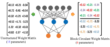
Figure 1. Block-circulant Matrices for weight representation.

As an effort to achieve the three goals, we propose CirCNN, a principled approach to represent weights and process neural networks using block-circulant matrices (pan2012structured, ). The concept of the block-circulant matrix compared to the ordinary unstructured matrix is shown in Fig. 1. In a square circulant matrix, each row (or column) vector is the circulant reformat of the other row (column) vectors. A non-squared matrix could be represented by a set of square circulant submatrices (blocks). Therefore, by representing a matrix with a vector, the first benefit of CirCNN is storage size reduction. In Fig. 1, the unstructured $6\times 3$ weight matrix (on the left) holds 18 parameters. Suppose we can represent the weights using two $3\times 3$ circulant matrices (on the right), we just need to store 6 parameters, easily leading to 3x model size reduction. Intuitively, the reduction ratio is determined by the block size of the circulant submatrices: larger block size leads to high compression ratio. In general, the storage complexity is reduced from O($n^{2}$) to O($n$).

The second benefit of CirCNN is computational complexity reduction. We explain the insights using a fully-connected layer of DNN, which can be represented as $\bf{y}=\psi(\bf{W}\bf{x}+\mathbf{\theta})$, where vectors $\bf{x}$ and $\bf{y}$ represent the outputs of all neurons in the previous layer and the current layer, respectively; $\bf{W}$ is the $m$-by-$n$ weight matrix; and $\psi(\cdot)$ is activation function. When $\bf{W}$ is a block-circulant matrix, the Fast Fourier Transform (FFT)-based fast multiplication method can be utilized, and the computational complexity is reduced from O($n^{2}$) to O($n\log n$).

It is important to understand that CirCNN incurs no conversion between the unstructured weight matrices and block-circulant matrices. Instead, we assume that the layers can be represented by block-circulant matrices and the training generates a vector for each circulant submatrix. The fundamental difference is that: the current approaches apply various compression techniques (e.g., pruning) on the unstructured weight matrices and then retrain the network; while CirCNN directly trains the network assuming block-circulant structure. This leads to two advantages. First, the prior work can only reduce the model size by a heuristic factor, depending on the network, while CirCNN provides the adjustable but fixed reduction ratio. Second, with the same FFT-based fast multiplication, the computational complexity of training is also reduced from O($n^{2}$) to O($n\log n$). Unfortunately, the prior work does not reduce (or even increase) training complexity.

Due to the storage and computational complexity reduction, CirCNN is clearly attractive. The only question is: can a network really be represented by block-circulant matrices with no (or negligible) accuracy loss? This question is natural, because with the much less weights in the vectors, the network may not be able to approximate the function of the network with unstructured weight matrices. Fortunately, the answer to the question is YES. CirCNN is mathematically rigorous: we have developed a theoretical foundation and formal proof showing that the DNNs represented by block-circulant matrices can converge to the same “effectiveness” as DNNs without compression, fundamentally distinguishing our method from prior arts. The outline of the proof is discussed in Section 3.3 and the details are provided in technical reports (proof_simple, ; proof, ).

Based on block-circulant matrix-based algorithms, we propose CirCNN architecture, — a universal DNN inference engine that can be implemented in various hardware/software platforms with configurable network architecture (e.g., layer type, size, scales, etc.). Applying CirCNN to neural network accelerators enables notable architectural innovations. 1) Due to its recursive property and its intrinsic role in CirCNN, FFT is implemented as the basic computing block. It ensures universal and small-footprint implementations. 2) Pipelining and parallelism optimizations. Taking advantage of the compressed but regular network structures, we aggressively apply inter-level and intra-level pipelining in the basic computing block. Moreover, we can conduct joint-optimizations considering parallelization degree, performance and power consumption. 3) Platform-specific optimizations focusing on weight storage and memory management.

To demonstrate the performance and energy efficiency, we test CirCNN architecture in three platforms: FPGA, ASIC and embedded processors. Our results show that CirCNN architecture achieves very high energy efficiency and performance with a small hardware footprint. Based on the FPGA implementation and ASIC synthesis results, CirCNN achieves 6 - 102X energy efficiency improvements compared with the best state-of-the-art results.

2. Background and Motivation

2.1. Deep Neural Networks

Deep learning systems can be constructed using different types of architectures, including deep convolutional neural networks (DCNNs), deep belief networks (DBNs), and recurrent neural networks (RNNs). Despite the differences in network structures and target applications, they share the same construction principle: multiple functional layers are cascaded together to extract features at multiple levels of abstraction (lee2009convolutional, ; karpathy2014large, ; yu2011deep, ). Fig. 2 illustrates the multi-layer structure of an example DCNN, which consists of a stack of fully-connected layers, convolutional layers, and pooling layers. These three types of layers are fundamental in deep learning systems.

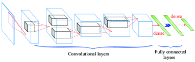
Figure 2. Multi-layer structure of an example DCNN.

The fully-connected (FC) layer is the most storage-intensive layer in DNN architectures (qiu2016going, ; zhang2016caffeine, ) since its neurons are fully connected with neurons in the previous layer. The computation procedure of a FC layer consists of matrix-vector arithmetics (multiplications and additions) and transformation by the activation function, as described as follows:

(1) $$\bf{y}=\psi(\bf{W}\bf{x}+\mathbf{\theta})$$

where $\textbf{W}\in\mathbb{R}^{m\times n}$ is the weight matrix of the synapses between this FC layer (with $m$ neurons) and its previous layer (with $n$ neurons); $\mathbf{\theta}\in\mathbb{R}^{m}$ is the bias vector; and $\psi(\cdot)$ is the activation function. The Rectified Linear Unit (ReLU) $\psi(x)=\max(0,x)$ is the most widely utilized in DNNs.

The convolutional (CONV) layer, as the name implies, performs a two-dimensional convolution to extract features from its inputs that will be fed into subsequent layers for extracting higher-level features. A CONV layer is associated with a set of learnable filters (or kernels) (lecun1998gradient, ), which are activated when specific types of features are found at some spatial positions in inputs. A filter-sized moving window is applied to the inputs to obtain a set of feature maps, calculating the convolution of the filter and inputs in the moving window. Each convolutional neuron, representing one pixel in a feature map, takes a set of inputs and the corresponding filter weights to calculate the inner-product. Given input feature map X and the $r\times r$-sized filter (i.e., the convolutional kernel) F, the output feature map Y is calculated as

(2) $$y_{a,b}=\sum_{i=1}^{r}\sum_{j=1}^{r}x_{a+i-1,b+j-1}\times f_{i,j},$$

where $y_{a,b}$, $x_{a+i-1,b+j-1}$, and $f_{i,j}$ are elements in Y, X, and F, respectively. Multiple convolutional kernels can be adopted to extract different features in the same input feature map. Multiple input feature maps can be convolved with the same filter and results are summed up to derive a single feature map.

The pooling (POOL) layer performs a subsampling operation on the extracted features to reduce the data dimensions and mitigate overfitting issues. Here, the subsampling operation on the inputs of pooling layer can be realized by various non-linear operations, such as max, average or L2-norm calculation. Among them, the max pooling is the dominant type of pooling strategy in state-of-the-art DCNNs due to the higher overall accuracy and convergence speed (han2017ese, ; chen2017eyeriss, ).

Among these three types of layers, the majority of computation occurs in CONV and FC layers, while the POOL layer has a relatively lower computational complexity of O($n$). The storage requirement of DNNs is due to the weight matrices W’s in the FC layers and the convolutional kernels F’s in CONV layers. As a result, the FC and CONV layers become the major research focuses on energy-efficient implementation and weight reduction of DNNs.

2.2. DNN Weight Storage Reduction and Acceleration

Mathematical investigations have demonstrated significant sparsity and margin for weight reduction in DNNs, a number of prior works leverage this property to reduce weight storage. The techniques can be classified into two categories. 1) Systematic methods (xue2013restructuring, ; liu2015eda, ; chung2016simplifying, ) such as Singular Value Decomposition (SVD). Despite being systematic, these methods typically exhibit a relatively high degradation in the overall accuracy (by 5%-10% at 10$\times$ compression). 2) Heuristic pruning methods (han2015deep, ; han2015learning, ; hwang2014fixed, ) use heuristic weight together with weight quantization. These method could achieve a better parameter reductions, i.e., 9$\times$-13$\times$ (han2015deep, ; han2015learning, ), and a very small accuracy degradation. However, the network structure and weight storage after pruning become highly irregular (c.f. Fig. 3) and therefore indexing is always needed, which undermines the compression ratio and more importantly, the performance improvement.

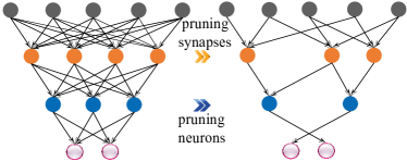
Figure 3. Illustration of the heuristic weight pruning methods.

Besides the pros and cons of the two approaches, the prior works share the following common limitations: 1) mainly focusing on weight reduction rather than computational complexity reduction; 2) only reducing the model size by a heuristic factor instead of reducing the Big-O complexity; and 3) performing weight pruning or applying matrix transformations based on a trained DNN model, thereby adding complexity to the training process. The third item is crucial because it may limit the scalability of future larger-scale deep learning systems.

2.3. FFT-Based Methods

LeCun et al. has proposed using FFTs to accelerate the computations in the CONV layers, which applies only to a single filter in the CONV layer (mathieu2013fast, ). It uses FFT to calculate the traditional inner products of filters and input feature maps, and can achieve speedup for large filter sizes (which is less common in state-of-the-art DCNNs (he2016deep, )). The underlying neural network structure and parameters remain unchanged. The speedup is due to filter reuse and it cannot achieve either asymptotic speedup in big-O notation or weight compressions (in fact additional storage space is needed).

The work most closely related to CirCNN is (cheng2015exploration, ). It proposed to use circulant matrix in the inference and training algorithms. However, it has a number of limitations. First, it only applied to FC layers, but not CONV layer. It limits the potential gain in weight reduction and performance. Second, it uses a single circulant matrix to represent the weights in the whole FC layer. Since the number of input and output neurons are usually not the same, this method leads to the storage waste due to the padded zeros (to make the circulant matrix squared).

2.4. Novelty of CirCNN

Compared with LeCun et al. (mathieu2013fast, ), CirCNN is fundamentally different as it achieves asymptotic speedup in big-O notation and weight compression simultaneously. Compared with (cheng2015exploration, ), CirCNN generalizes in three significant and novel aspects.

Supporting both FC and CONV layers. Unlike FC layers, the matrices in CONV layers are small filters (e.g., $3\times 3$). Instead of representing each filter as a circulant matrix, CirCNN exploits the inter-filter sparsity among different filters. In another word, CirCNN represents a matrix of filters, where input and output channels are the two dimensions, by a vector of filters. The support for CONV layers allow CirCNN to be applied in the whole network.

Block-circulant matrices. To mitigate the inefficiency due to the single large circulant matrix used in (cheng2015exploration, ), CirCNN uses block-circulant matrices for weight representation. The benefits are two-fold. First, it avoids the wasted storage/computation due to zero padding when the numbers of inputs and outputs are not equal. Second, it allows us to derive a fine-grained tradeoff between accuracy and compression/acceleration. Specifically, to achieve better compression ratio, larger block size should be used, however, it may lead to more accuracy degradation. The smaller block sizes provide better accuracy, but less compression. There is no compression if the block size is 1.

Mathematical rigorousness. Importantly, we perform theoretical analysis to prove that the “effectiveness” of block-circulant matrix-based DNNs will (asymptotically) approach that of original networks without compression. The theoretical proof also distinguishes the proposed method with prior work. The outline of the proof is discussed in Section 3.3 and the details are provided in reports (proof_simple, ; proof, ).

Fig. 4 illustrates the difference between the baseline (cheng2015exploration, ) and CirCNN. The baseline method (a) formulates a large, square circulant matrix by zero padding for FC layer weight representation when the numbers of inputs and outputs are not equal. In contrast, CirCNN (b) uses the block-circulant matrix to avoid storage waste and achieve a fine-grained tradeoff of accuracy and compression/acceleration.

Overall, with the novel techniques of CirCNN, at algorithm level, it is possible to achieve the simultaneous and significant reduction of both computational and storage complexity, for both inference and training.

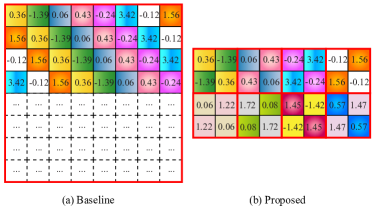
Figure 4. Baseline (cheng2015exploration, ) and CirCNN. The baseline method (a) formulates a large, square circulant matrix for FC layer weight representation when the numbers of inputs and outputs are not equal, whereas the proposed method (b) uses the block-circulant matrix to achieve a fine-grained tradeoff of accuracy and compression/acceleration.

3. CirCNN: Algorithms and Foundation

3.1. FC Layer Algorithm

The key idea of block-circulant matrix-based FC layers is to partition the original arbitrary-size weight matrix $\textbf{W}\in\mathbb{R}^{m\times n}$ into 2D blocks of square sub-matrices, and each sub-matrix is a circulant matrix. The insights are shown in Fig.  5. Let $k$ denote the block size (size of each sub-matrix) and assume there are $p\times q$ blocks after partitioning $\mathbf{W}$, where $p=m\div k$ and $q=n\div k$. Then $\mathbf{W}=[\mathbf{W}_{ij}]$, $i\in\{1\dots p\}$, $j\in\{1\dots q\}$. Correspondingly, the input $\mathbf{x}$ is also partitioned as $\mathbf{x}=[\mathbf{x}^{T}_{1},\mathbf{x}^{T}_{2},\dots,\mathbf{x}^{T}_{q}]^{T}$. Then, the forward propagation process in the inference phase is given by (with bias and ReLU omitted):

(3) $$\mathbf{a}=\mathbf{Wx}=\begin{bmatrix}\sum_{j=1}^{q}\mathbf{W}_{1j}\mathbf{x}_{j}\\ \sum_{j=1}^{q}\mathbf{W}_{2j}\mathbf{x}_{j}\\ \dots\\ \sum_{j=1}^{q}\mathbf{W}_{pj}\mathbf{x}_{j}\end{bmatrix}=\begin{bmatrix}\mathbf{a}_{1}\\ \mathbf{a}_{2}\\ \dots\\ \mathbf{a}_{p}\end{bmatrix},$$

where $\mathbf{a}_{i}\in\mathbb{R}^{k}$ is a column vector. Assume each circulant matrix $\mathbf{W}_{ij}$ is defined by a vector $\mathbf{w}_{ij}$, i.e., $\mathbf{w}_{ij}$ is the first row vector of $\mathbf{W}_{ij}$. Then according to the circulant convolution theorem (pan2012structured, ; bini1996polynomial, ), the calculation of $\mathbf{W}_{ij}\mathbf{x}_{j}$ can be performed as $\text{IFFT}\big{(}\text{FFT}(\mathbf{w}_{ij})\circ\text{FFT}(\mathbf{x}_{j})\big{)}$, where $\circ$ denotes element-wise multiplications. The operation procedure is shown on the right of Fig.  5. For the inference phase, the computational complexity of this FC layer will be $O(pqk\log k)$, which is equivalent to $O(n\log n)$ for small $p$, $q$ values. Similarly, the storage complexity will be $O(pqk)$ because we only need to store $\mathbf{w}_{ij}$ or $\text{FFT}(\mathbf{w}_{ij})$ for each sub-matrix, which is equivalent to $O(n)$ for small $p$, $q$ values. Therefore, the simultaneous acceleration and model compression compared with the original DNN can be achieved for the inference process. Algorithm 1 illustrates the calculation of $\bf{Wx}$ in the inference process in the FC layer of CirCNN.

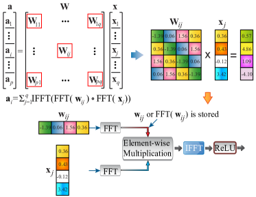
Figure 5. Illustration of the calculation of $\bf{Wx}$ in the inference process of FC layer.

Input: $\mathbf{w}_{ij}$’s, $\mathbf{x}$, $p$, $q$, $k$

Output: $\mathbf{a}$

Initialize $\mathbf{a}$ with zeros.

for $i\leftarrow 1$ until p do

      for $j\leftarrow 1$ until q do

           $\mathbf{a}_{i}$ $\leftarrow$ $\mathbf{a}_{i}$ + $\text{IFFT}(\text{FFT}(\mathbf{w}_{ij})\circ\text{FFT}(\mathbf{x}_{j}))$

          

           end for

          

           end for

          return $\mathbf{a}$

Algorithm 1 Forward propagation process in the FC layer of CirCNN

Next, we consider the backward propagation process in the training phase. Let $a_{il}$ be the $l$-th output element in $\mathbf{a}_{i}$, and $L$ denote the loss function. Then by using the chain rule we can derive the backward propagation process as follows:

(4) $$\frac{\partial L}{\partial\mathbf{w}_{ij}}=\sum_{l=1}^{k}\frac{\partial L}{\partial a_{il}}\frac{\partial a_{il}}{\partial\mathbf{w}_{ij}}=\frac{\partial L}{\partial\mathbf{a}_{i}}\frac{\partial\mathbf{a}_{i}}{\partial\mathbf{w}_{ij}},$$

(5) $$\frac{\partial L}{\partial\mathbf{x}_{j}}=\sum_{i=1}^{p}\sum_{l=1}^{k}\frac{\partial L}{\partial a_{il}}\frac{\partial a_{il}}{\partial\mathbf{x}_{j}}=\sum_{i=1}^{p}\frac{\partial L}{\partial\mathbf{a}_{i}}\frac{\partial\mathbf{a}_{i}}{\partial\mathbf{x}_{j}}.$$

We have proved that $\frac{\partial\mathbf{a}_{i}}{\partial\mathbf{w}_{ij}}$ and $\frac{\partial\mathbf{a}_{i}}{\partial\mathbf{x}_{j}}$ are block-circulant matrices. Therefore, $\frac{\partial L}{\partial\mathbf{w}_{ij}}$ and $\frac{\partial L}{\partial\mathbf{a}_{i}}\frac{\partial\mathbf{a}_{i}}{\partial\mathbf{x}_{j}}$ can be calculated as the “FFT$\rightarrow$element-wise multiplication$\rightarrow$IFFT” procedure and is equivalent to $O(n\log n)$ computational complexity per layer. Algorithm 2 illustrates backward propagation process in the FC layer of CirCNN.

Input: $\frac{\partial L}{\partial\mathbf{a}}$, $\mathbf{w}_{ij}$’s, $\mathbf{x}$, $p$, $q$, $k$

Output: $\frac{\partial L}{\partial\mathbf{w}_{ij}}$’s, $\frac{\partial L}{\partial\mathbf{x}}$

Initialize $\frac{\partial L}{\partial\mathbf{w}_{ij}}$’s and $\frac{\partial L}{\partial\mathbf{x}}$ with zeros.

for $i\leftarrow 1$ until p do

      for $j\leftarrow 1$ until q do

           $\frac{\partial L}{\partial\mathbf{w}_{ij}}\leftarrow\text{IFFT}(\text{FFT}(\frac{\partial L}{\partial\mathbf{a}_{i}})\circ\text{FFT}(\mathbf{x^{\prime}}_{j}))$

           $\frac{\partial L}{\partial\mathbf{x}_{j}}\leftarrow\frac{\partial L}{\partial\mathbf{x}_{j}}+\text{IFFT}(\text{FFT}(\frac{\partial L}{\partial\mathbf{a}_{i}})\circ\text{FFT}(\mathbf{w}_{ij}))$

          

           end for

          

           end for

          return $\frac{\partial L}{\partial\mathbf{w}_{ij}}$’s, $\frac{\partial L}{\partial\mathbf{x}}$

Algorithm 2 Backward propagation process in the FC layer of CirCNN

In CirCNN, the inference and training constitute an integrated framework where the reduction of computational complexity can be gained for both. We directly train the vectors $\mathbf{w}_{ij}$’s, corresponding to the circulant sub-matrices $\mathbf{W}_{ij}$’s, in each layer using Algorithm 2. Clearly, the network after such training procedure naturally follows the block-circulant matrix structure. It is a key advantage of CirCNN compared with prior works which require additional steps on a trained neural network.

3.2. CONV Layer Algorithm

In practical DNN models, the CONV layers are often associated with multiple input and multiple output feature maps. As a result, the computation in the CONV layer can be expressed in the format of tensor computations as below:

(6) $$\mathcal{Y}(x,y,p)=\sum_{i=1}^{r}\sum_{j=1}^{r}\sum_{c=1}^{C}\mathcal{F}(i,j,c,p)\mathcal{X}(x+i-1,y+j-1,c),$$

where $\mathcal{X}\in\mathbb{R}^{W\times H\times C}$, $\mathcal{Y}\in\mathbb{R}^{(W-r+1)\times(H-r+1)\times P}$, $\mathcal{F}\in\mathbb{R}^{r\times r\times C\times P}$ represent the input, output, and weight “tensors” of the CONV layer, respectively. Here, $W$ and $H$ are the spatial dimensions of the input maps, $C$ is the number of input maps, $r$ is the size of the convolutional kernel, and $P$ is the number of output maps.

We generalize the concept of “block-circulant structure” to the rank-4 tensor ($\mathcal{F}$) in the CONV layer, i.e., all the slices of the form $\mathcal{F}(\cdot,\cdot,i,j)$ are circulant matrices. Next, we reformulate the inference and training algorithms of the CONV layer to matrix operations. We use the inference process as an example, and the training process can be formulated in a similar way.

Software tools such as Caffe provide an efficient methodology of transforming tensor-based operations in the CONV layer to matrix-based operations (jia2014caffe, ; vedaldi2015matconvnet, ), in order to enhance the implementation efficiency (GPUs are optimized for matrix operations.) Fig. 6 illustrates the application of the method to reformulate Eqn. (6) to the matrix multiplication $\mathbf{Y}=\mathbf{XF}$, where $\mathbf{X}\in\mathbb{R}^{(W-r+1)(H-r+1)\times Cr^{2}}$, $\mathbf{Y}\in\mathbb{R}^{(W-r+1)(H-r+1)\times P}$, and $\mathbf{F}\in\mathbb{R}^{Cr^{2}\times P}$.

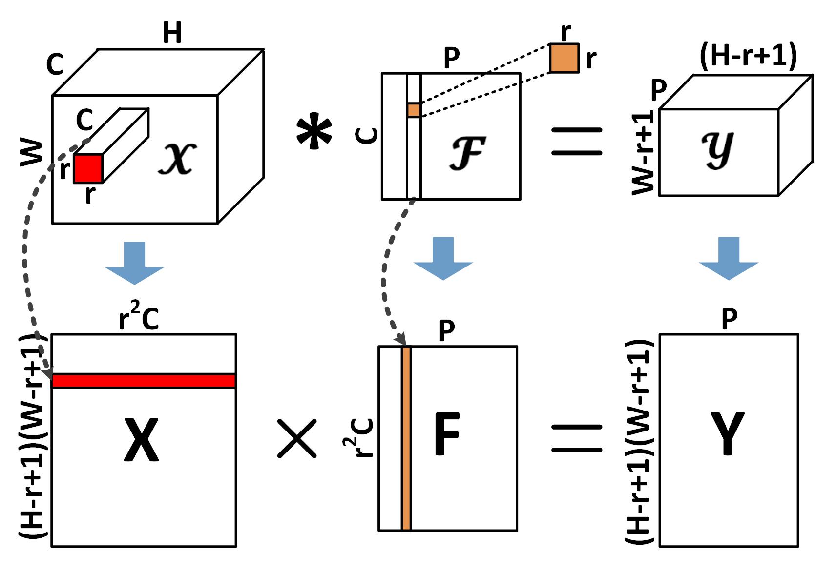
Figure 6. Reformulation of Eqn. (6) to matrix multiplication.

Recall that the slice of $\mathcal{F}(\cdot,\cdot,i,j)$ is a circulant matrix. Then according to the reshaping principle between $\mathcal{F}$ and $\mathbf{F}$, we have:

(7) $$f_{a+C(i-1)+Cr(j-1),b}=f_{C(i-1)+Cr(j-1),b-a},\forall a,b$$

which means $\mathbf{F}$ is actually a block-circulant matrix. Hence the fast multiplication approach for block circulant matrix, as the “FFT$\rightarrow$ component-wise multiplication $\rightarrow$IFFT” procedure, can now be applied to accelerate $\mathbf{Y}=\mathbf{XF}$, thereby resulting in the acceleration of (6). With the use of the proposed approach, the computational complexity for (6) is reduced from O($WHr^{2}CP$) to O($WHQ\log Q$), where $Q=\max(r^{2}C,P)$.

3.3. Outline of Theoretical Proof

With the substantial reduction of weight storage and computational complexities, we attempt to prove that the proposed block-circulant matrix-based framework will consistently yield the similar overall accuracy compared with DNNs without compression. Only testing on existing benchmarks is insufficient given the rapid emergence of new application domains, DNN models, and data-sets. The theoretical proof will make the proposed method theoretically rigorous and distinct from prior work.

In the theory of neural networks, the “effectiveness” is defined using the universal approximation property, which states that a neural network should be able to approximate any continuous or measurable function with arbitrary accuracy provided that an enough large number of parameters are available. This property provides the theoretical guarantee of using neural networks to solve machine learning problems, since machine learning tasks can be formulated as finding a proper approximation of an unknown, high-dimensional function. Therefore, the goal is to prove the universal approximation property of block circulant matrix-based neural networks, and more generally, for arbitrary structured matrices satisfying the low displacement rank $\gamma$. The detailed proofs for the block circulant matrix-based networks and general structured matrix-based ones are provided in the technical reports (proof_simple, ; proof, ).

The proof of the universal approximation property for block circulant matrix-based neural networks is briefly outlined as follows: Our objective is to prove that any continuous or measurable function can be approximated with arbitrary accuracy using a block-circulant matrix-based network. Equivalently, we aim to prove that the function space achieved by block-circulant matrix-based neural networks is dense in the space of continuous or measurable functions with the same inputs. An important property of the activation function, i.e., the component-wise discriminatory property, is proved. Based on this property, the above objective is proved using proof by contradiction and Hahn-Banach Theorem (narici1997hahn, ).

We have further derived an approximation error bound of O($1/n$) when the number of neurons in the layer $n$ is limited, with details shown in (proof, ). It implies that the approximation error will reduce with an increasing $n$, i.e., an increasing number of neurons/inputs in the network. As a result, we can guarantee the universal “effectiveness” of the proposed framework on different DNN types and sizes, application domains, and hardware/software platforms.

3.4. Compression Ratio and Test Accuracy

In this section, we apply CirCNN to different DNN models in software and investigate the weight compression ratio and accuracy. Fig. 7 (a) and (b) show the weight storage (model size) reduction in FC layer and test accuracy on various image recognition datasets and DCNN models: MNIST (LeNet-5), CIFAR-10, SVHN, STL-10, and ImageNet (using AlexNet structure) (krizhevsky2012imagenet, ; netzer2011reading, ; krizhevsky2009learning, ; coates2010analysis, ; deng2012mnist, )). Here, 16-bit weight quantization is adopted for model size reduction. The baselines are the original DCNN models with unstructured weight matrices using 32-bit floating point representations. We see that block-circulant weight matrices enable 400$\times$-4000+$\times$ reduction in weight storage (model size) in corresponding FC layers. This parameter reduction in FC layers is also observed in (cheng2015exploration, ). The entire DCNN model size (excluding softmax layer) is reduced by 30-50$\times$ when only applying block-circulant matrices to the FC layer (and quantization to the overall network). Regarding accuracy, the loss is negligible and sometimes the compressed models even outperform the baseline models.

Fig. 7 (c) illustrates the further application of block-circulant weight matrices to the CONV layers on MNIST (LeNet-5), SVHN, CIFAR-10, and ImageNet (AlexNet structure) datasets, when the accuracy degradation is constrained to be 1-2% by optimizing the block size. Again 16-bit weight quantization is adopted, and softmax layer is excluded. The 16-bit quantization also contributes to 2$\times$ reduction in model size. In comparison, the reductions of the number of parameters in (han2015deep, ; han2015learning, ) are 12$\times$ for LeNet-5 (on MNIST dataset) and 9$\times$ for AlexNet. Moreover, another crucial property of CirCNN is that the parameter storage after compression is regular, whereas (han2015deep, ; han2015learning, ) result in irregular weight storage patterns. The irregularity requires additional index per weight and significantly impacts the available parallelism degree. From the results, we clearly see the significant benefit and potential of CirCNN: it could produce highly compressed models with regular structure. CirCNN yields more reductions in parameters compared with the state-of-the-art results for LeNet-5 and AlexNet. In fact, the actual gain could even be higher due to the indexing requirements of (han2015deep, ; han2015learning, ).

We have also performed testing on other DNN models such as DBN, and found that CirCNN can achieve similar or even higher compression ratio, demonstrating the wide application of block-circulant matrices. Moreover, a 5$\times$ to 9$\times$ acceleration in training can be observed for DBNs, which is less phenomenal than the model reduction ratio. This is because GPUs are less optimized for FFT operation than matrix-vector multiplications.

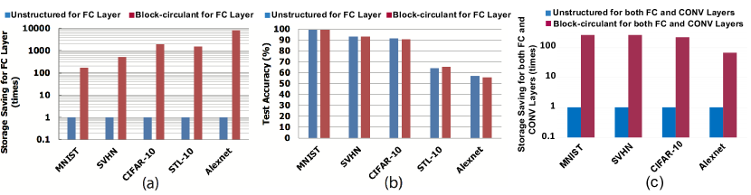
Figure 7. (a) Storage saving and (b) test accuracy after using block-circulant FC layer for DCNN models on different datasets. (c) Storage saving after using both block-circulant FC layer and block-circulant CONV layer for DCNNs on MNIST, SVHN, CIFAR-10, and ImageNet datasets.

4. CirCNN Architecture

Based on block-circulant matrix-based algorithms, we propose CirCNN architecture, — a universal DNN inference engine that can be implemented in various hardware/software platforms with configurable network architecture (e.g., layer type, size, scales, etc.).

Applying CirCNN to neural network accelerators enables notable architectural innovations. 1) Due to its recursive property and its intrinsic role in CirCNN, FFT is implemented as the basic computing block (Section 4.1). It ensures universal and small-footprint implementations. 2) Pipelining and parallelism optimizations (Section 4.3). Taking advantage of the compressed but regular network structures, we aggressively apply inter-level and intra-level pipelining in the basic computing block. Moreover, we can conduct joint-optimizations considering parallelization degree, performance and power consumption. 3) Platform-specific optimizations focusing on weight storage and memory management.(Section 4.4).

4.1. Recursive Property of FFT: the Key to Universal and Small Footprint Design

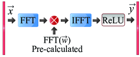
Figure 8. The “FFT$\rightarrow$component-wise multiplication$\rightarrow$IFFT” procedure.

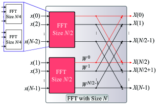
Figure 9. Illustration of the recursive property of FFT.

In CirCNN, the “FFT$\rightarrow$component-wise multiplication $\rightarrow$IFFT” in Fig. 8 is a universal procedure used in both FC and CONV layers, for both inference and training processes, and for different DNN models. We consider FFT as the key computing kernel in CirCNN architecture due to its recursive property. It is known that FFT can be highly efficient with O($n\log n$) computational complexity, and hardware implementation of FFT has been investigated in (salehi2013pipelined, ; chang2003efficient, ; cheng2007high, ; garrido2009pipelined, ; garrido2009pipelined, ; ayinala2013place, ; ayinala2013fft, ). The recursive property states that the calculation of a size-$n$ FFT (with $n$ inputs and $n$ outputs) can be implemented using two FFTs with size $n/2$ plus one additional level of butterfly calculation, as shown in Fig. 9. It can be further decomposed to four FFTs with size $n/4$ with two additional levels.

The recursive property of FFT is the key to ensure a universal and reconfigurable design which could handle different DNN types, sizes, scales, etc. It is because: 1) A large-scale FFT can be calculated by recursively executing on the same computing block and some additional calculations; and 2) IFFT can be implemented using the same structure as FFT with different preprocessing procedure and parameters (salehi2013pipelined, ). It also ensures the design with small footprint, because: 1) Multiple small-scale FFT blocks can be multiplexed and calculate a large-scale FFT with certain parallelism degree; and 2) The additional component-wise multiplication has O($n$) complexity and relatively small hardware footprint.

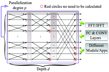
Figure 10. The Basic Computing Block.

Actual hardware systems, such as FPGA or ASIC designs, pose constraints on parallel implementation due to hardware footprint and logic block/interconnect resource limitations. As a result, we define the basic computing block with a parallelization degree $p$ and depth $d$ (of butterfly computations), as shown in Fig. 10. A butterfly computation in FFT comprises cascade connection of complex number-based multiplications and additions (oppenheim1999discrete, ; altera2010megacore, ). The basic computing block is responsible for implementing the major computational tasks (FFT and IFFTs). An FFT operation (with reconfigurable size) is done by decomposition and iterative execution on the basic computing blocks.

Compared with conventional FFT calculation, we simplify the FFT computing based on the following observation: Our inputs of the deep learning system are from actual applications and are real values without imaginary parts. Therefore, the FFT result of each level will be a symmetric sequence except for the base component (salehi2013pipelined, ). As an example shown in the basic computing block shown in Fig. 10, the partial FFT outcomes at each layer of butterfly computations will be symmetric, and therefore, the outcomes in the red circles do not need to be calculated and stored as partial outcomes. This observation can significantly reduce the amount of computations, storage of partial results, and memory traffic.

4.2. Overall Architecture

The overall CirCNN architecture is shown in Fig. 11, which includes the basic computing block, the peripheral computing block, the control subsystem, the memory subsystem, and I/O subsystem (I/O buffers). The basic computing block is responsible for the major FFT and IFFT computations. The peripheral computing block is responsible for performing component-wise multiplication, ReLU activation, pooling etc., which require lower (linear) computational complexity and hardware footprint. The implementations of ReLU activation and pooling are through comparators and have no inherent difference compared with prior work (chen2014dadiannao, ; han2016eie, ). The control subsystem orchestrates the actual FFT/IFFT calculations on the basic computing block and peripheral computing block. Due to the different sizes of CONV layer, FC layer and different types of deep learning applications, the different setting of FFT/IFFT calculations is configured by the control subsystem. The memory subsystem is composed of ROM, which is utilized to store the coefficients in FFT/IFFT calculations (i.e., the $W_{n}^{i}$ values including both real and imaginary parts); and RAM, which is used to store weights, e.g., the FFT results $\text{FFT}(\mathbf{w}_{ij})$. For ASIC design, a memory hierarchy may be utilized and carefully designed to ensure good performance.

We use 16-bit fixed point numbers for input and weight representations, which is common and widely accepted to be enough accurate for DNNs (chen2014dadiannao, ; han2016eie, ; chen2017eyeriss, ; judd2016stripes, ). Furthermore, it is pointed out (han2015deep, ; lin2016fixed, ) that inaccuracy caused by quantization is largely independent of inaccuracy caused by compression and the quantization inaccuracy will not accumulate significantly for deep layers.

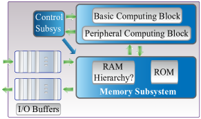
Figure 11. CirCNN Architecture.

4.3. Pipelining and Parallelism

Thanks to the regular block-circulant matrix structure, effective pipelining can be utilized to achieve the optimal tradeoff between energy efficiency and performance (throughput). CirCNN architecture considers two pipelining techniques as shown in Fig. 12. In inter-level pipelining, each pipeline stage corresponds to one level in the basic computing block. In intra-level pipelining, additional pipeline stage(s) will be added within each butterfly computation unit, i.e., by deriving the optimal stage division in the cascade connection of complex number-based multiplication and additions. The proper selection of pipelining scheme highly depends on the target operating frequency and memory subsystem organization. In the experimental prototype, we target at a clock frequency around 200MHz (close to state-of-the-art ASIC tapeouts of DCNNs (chen2017eyeriss, ; desoli201714, ; moons201714, )), and therefore the inter-level pipelining with a simpler structure will be sufficient for efficient implementations.

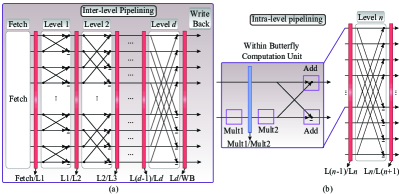
Figure 12. The (a) inter-level and (b) intra-level pipelining techniques.

Based on the definition of $p$ (parallelization degree) and $d$ (parallelization depth), larger $p$ and $d$ values indicate higher level of parallelism and therefore will lead to higher performance and throughput, but also with higher hardware cost/footprint. A larger $d$ value would also result in less memory accesses at the cost of higher control complexity. We derive the optimal $p$ and $d$ values by optimizing an overall metric $M\big{(}Perf(p,d),$ $Power(p,d)\big{)}$ as a suitable function of (average) performance and power consumption. The performance $Perf(p,d)$ will be an increasing function of $p$ and $d$ but also depends on the platform specifications, and the target type and size of DNN models (averaged over a set of learning models). The power consumption $Power(p,d)$ is a close-to-linear function of $pd$ accounting for both static and dynamic components of power dissipation. The optimization of $p$ and $d$ is constrained by the compute and memory hardware resource limits as well as memory and I/O bandwidth constraints. The proposed algorithm for design optimization is illustrated in Algorithm 3, which sets $p$ as optimization priority in order not to increase control complexity. This algorithm depends on the accurate estimation of performance and power consumption at each design configuration.

We provide an example of design optimization and effects assuming a block size of 128 for FPGA-based implementation (Cyclone V). Because of the low operating frequency, increasing the $p$ value from 16 to 32 while maintaining $d=1$ only increases power consumption by less than 10%. However, the performance can be increased by 53.8% with a simple pipelining control. Increasing $d$ from 1 to 2 results in even less increase in power of 7.8%, with performance increase of 62.2%. The results seem to show that increasing $d$ is slightly more beneficial because of the reduced memory access overheads. However, a $d$ value higher than 3 will result in high control difficulty and pipelining bubbles, whereas $p$ can be increased with the same control complexity thanks to the high bandwidth of block memory in FPGAs. As a result, we put $p$ as the optimization priority in Algorithm 3.

Optimize parallel degree $p$:

 Derive upper bound of $p$ based on memory bandwidth

  -limit & hardware resource limit;

 Use ternary search for $p$:

  Estimate $M\big{(}Perf(p,d),$ $Power(p,d)\big{)}$ assuming $d=1$;

Optimize depth $d$ using the ternary search method, based on the derived $p$ value.

Algorithm 3 The proposed algorithm for design optimization of basic computing block

4.4. Platform-Specific Optimizations

Based on the generic CirCNN architecture, this section describes platform-specific optimizations on the FPGA-based and ASIC-based hardware platforms. We focus on weight storage and memory management, in order to simplify the design and achieve higher energy efficiency and performance.

FPGA Platform. The key observation is that the weight storage requirement of representative DNN applications can be (potentially) met by the on-chip block memory in state-of-the-art FPGAs. As a representative large-scale DCNN model for ImageNet application, the whole AlexNet (krizhevsky2012imagenet, ) results in only around 4MB storage requirement after (i) applying block-circulant matrices only to FC layers, and (ii) using 16-bit fixed point numbers that results in negligible accuracy loss. Such storage requirement can be fulfilled by the on-chip block memory of state-of-the-art FPGAs such as Intel (former Altera) Stratix, Xilinx Virtex-7, etc., which consist of up to tens of MBs on-chip memory (link1, ; link2, ). Moreover, when applying block-circulant matrices also to CONV layers, the storage requirement can be further reduced to 2MB or even less (depending on the block size and tolerable accuracy degradation). Then, the storage requirement becomes comparable with the input size and can be potentially supported by low-power and high energy-efficiency FPGAs such as Intel (Altera) Cyclone V or Xilinx Kintex-7 FPGAs. A similar observation holds for other applications (e.g., the MNIST data-set (deng2012mnist, )), or different network models like DBN or RNN. Even for future larger-scale applications, the full model after compression will (likely) fit in an FPGA SoC leveraging the storage space of the integrated ARM core and DDR memory (link1, ; link2, ). This observation would make the FPGA-based design significantly more efficient.

In state-of-the-art FPGAs, on-chip memory is organized in the form of memory blocks, each with certain capacity and bandwidth limit. The number of on-chip memory blocks represents a proper tradeoff between the lower control complexity (with more memory blocks) and the higher energy efficiency (with fewer memory blocks), and thus should become an additional knob for design optimizations. State-of-the-art FPGAs are equipped with comprehensive DSP resources such as $18\times 18$ or variable-size multipliers (link1, ; link2, ), which are effectively exploited for performance and energy efficiency improvements.

ASIC platform. We mainly investigate two aspects in the memory subsystem: 1) the potential memory hierarchy and 2) the memory bandwidth and aspect ratio. The representative deep learning applications require hundreds of KBs to multiple MBs memory storage depending on different compression levels, and we assume a conservative value of multiple MBs due to the universal and reconfigurable property of CirCNN architecture. The potential memory hierarchy structure depends strongly on the target clock frequency of the proposed system. Specifically, if we target at a clock frequency around 200MHz (close to state-of-the-art ASIC tapeouts of DCNNs (chen2017eyeriss, ; desoli201714, ; moons201714, )), then the memory hierarchy is not necessary because a single-level memory system can support such operating frequency. Rather, memory/cache reconfiguration techniques (wang2011dynamic, ; gordon2008phase, ) can be employed when executing different types and sizes of applications for performance enhancement and static power reduction. If we target at a higher clock frequency, say 800MHz, an effective memory hierarchy with at least two levels (L1 cache and main memory) becomes necessary because a single-level memory cannot accommodate such high operating frequency in this case. Please note that the cache-based memory hierarchy is highly efficient and results in very low cache miss rate because, prefetching (jouppi1998improving, ; dundas1997improving, ), the key technique to improve performance, will be highly effective due to the regular weight access patterns. The effectiveness of prefetching is due to the regularity in the proposed block-circulant matrix-based neural networks, showing another advantage over prior compression schemes. In our experimental results in the next section, we target at a lower clock frequency of 200MHz and therefore the memory hierarchy structure is not needed.

Besides the memory hierarchy structure, the memory bandwidth is determined by the parallelization degree $p$ in the basic computing block. Based on such configuration, the aspect ratio of the memory subsystem is determined. Because of the relatively high memory bandwidth requirement compared with the total memory capacity (after compression using block-circulant matrices), column decoders can be eliminated in general (weste2005cmos, ), thereby resulting in simpler layout and lower routing requirements.

5. Evaluation

In this section, we provide detailed experimental setups and results of the proposed universal inference framework on different platforms including FPGAs, ASIC designs, and embedded processors. Experimental results on representative benchmarks such as MNIST, CIFAR-10, SVHN, and ImageNet have been provided and we have conducted a comprehensive comparison with state-of-the-art works on hardware deep learning systems. Order(s) of magnitude in energy efficiency and performance improvements can be observed using the proposed universal inference framework.

5.1. FPGA-Based Testing

First, we illustrate our FPGA-based testing results using a low-power and low-cost Intel (Altera) Cyclone V 5CEA9 FPGA. The Cyclone V FPGA exhibits a low static power consumption less than 0.35W and highest operating frequency between 227MHz and 250MHz (but actual implementations typically have less than 100MHz frequency), making it a good choice for energy efficiency optimization of FPGA-based deep learning systems.

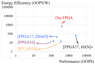
Figure 13. Comparison on performance and energy efficiency with state-of-the-art FPGA results.

Fig. 13 illustrates the comparison of performance (in giga operations per second, GOPS) and energy efficiency (in giga operations per Joule, GOPS/W) between the proposed and reference FPGA-based implementations. The FPGA implementation uses the AlexNet structure, a representative DCNN model with five CONV layers and three FC layers for the ImageNet applications (deng2009imagenet, ). The reference FPGA-based implementations are state-of-the-arts represented by [FPGA16] (qiu2016going, ), [ICCAD16] (zhang2016caffeine, ), [FPGA17, Han] (han2017ese, ), and [FPGA17, Zhao] (zhao2017accelerating, ). The reference works implement large-scale AlexNet, VGG-16, medium-scale DNN for CIFAR-10, or a custom-designed recurrent neural network (han2017ese, ). Note that we use equivalent GOPS and GOPS/W for all methods with weight storage compression, including ours. Although those references focus on different DNN models and structures, both GOPS and GOPS/W are general metrics that are independent of model differences. It is widely accepted in the hardware deep learning research to compare the GOPS and GOPS/W metrics between their proposed designs and those reported in the reference work, as shown in (qiu2016going, ; zhang2016caffeine, ; zhao2017accelerating, ). Please note that this is not entirely fair comparison because our implementation is layerwise implementation (some reference works implement end-to-end networks) and we extracts on-chip FPGA power consumptions.

In Fig. 13, we can observe the significant improvement achieved by the proposed FPGA-based implementations compared with prior arts in terms of energy efficiency, even achieving 11$\times$-16$\times$ improvement when comparing with prior work with heuristic model size reduction techniques (han2017ese, ; zhao2017accelerating, ) (reference (han2017ese, ) uses the heuristic weight pruning method, and (zhao2017accelerating, ) uses a binary-weighted neural network XOR-Net). When comparing with prior arts with a uncompressed (or partially compressed) deep learning system (qiu2016going, ; zhang2016caffeine, ), the energy efficiency improvement can reach 60-70$\times$. These results demonstrate a clear advantage of CirCNN using block-circulant matrices on energy efficiency. The performance and energy efficiency improvements are due to: 1) algorithm complexity reduction and 2) efficient hardware design, weight reduction, and elimination of weight accessing to the off-chip storage. The first source results in 10$\times$-20$\times$ improvement and the second results in 2$\times$-5$\times$. Please note that CirCNN architecture does not yield the highest throughput because we use a single low-power FPGA, while reference (han2017ese, ) uses a high-performance FPGA together with large off-chip DRAM on a custom-designed recurrent neural network. If needed, we can increase the number of FPGAs to process multiple neural networks in parallel, thereby improving the throughput without incurring any degradation in the energy efficiency.

Besides comparison with large-scale DCNNs with CirCNN architecture with state-of-the-art FPGA implementations, we also compare it with IBM TrueNorth neurosynaptic processor on a set of benchmark data sets including MNIST, CIFAR-10, and SVHN, which are all supported by IBM TrueNorth. This is a fair comparison because both the proposed system and IBM TrueNorth are end-to-end implementations. IBM TrueNorth (esser2016convolutional, ) is a neuromorphic CMOS chip fabricated in 28nm technology, with 4096 cores each simulating 256 programmable silicon neurons in a time-multiplexed manner. It implements Spiking Neural Networks, which is a bio-inspired type of neural networks and benefits from the ability of globally asynchronous implementations, but is widely perceived to achieve a lower accuracy compared with state-of-the-art DNN models. IBM TrueNorth exhibits the advantages of reconfigurability and programmability. Nevertheless, reconfigurability also applies to CirCNN architecture.

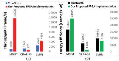
Figure 14. Comparison on (a) throughput and (b) energy efficiency between the proposed FPGA end-to-end implementation with TrueNorth reports (esser2015backpropagation, ; esser2016convolutional, ).

Fig. 14 compares the throughput and energy efficiency of FPGA-based implementations of CirCNN architecture and IBM TrueNorth on different benchmark data sets. The throughput and energy efficiency of IBM TrueNorth results are from (esser2015backpropagation, ; esser2016convolutional, ) ((esser2015backpropagation, ) for MNIST and (esser2016convolutional, ) for CIFAR-10 and SVHN), and we choose results from the low-power mapping mode using only a single TrueNorth chip for high energy efficiency. We can observe the improvement on the throughput for MNIST and SVHN data sets and energy efficiency on the same level of magnitude. The throughput of CIFAR-10 using the FPGA implementation of CirCNN is lower because 1) TrueNorth requires specific preprocessing of CIFAR-10  (esser2016convolutional, ) before performing inference, and 2) the DNN model we chose uses small-scale FFTs, which limits the degree of improvements. Besides, CirCNN architecture achieves the higher test accuracy in general: it results in very minor accuracy degradation compared with software DCNNs (cf. Fig. 7), whereas the low-power mode of IBM TrueNorth incurs higher accuracy degradation (esser2015backpropagation, ; esser2016convolutional, ). These results demonstrate the high effectiveness of CirCNN architecture because it is widely perceived that FPGA-based implementations will result in lower performance and energy efficiency compared with ASIC implementations, with benefits of a short development round and higher flexibility.

5.2. ASIC Designs Synthesis Results

We derive ASIC synthesis results of CirCNN architecture for large-scale DCNN implementations (AlexNet) and compare with state-of-the-art ASIC developments and synthesis results. The delay, power, and energy of our ASIC designs are obtained from synthesized RTL under Nangate 45nm process (nangate, ) using Synopsys Design Compiler. The memories are SRAM based and estimated using CACTI 5.3 (cacti, ). Fig. 15 illustrates the comparison results on ASIC-based implementations/synthesis with state-of-the-arts, which also target at large-scale deep learning systems. The reference ASIC implementations and synthesis results are represented by [EIE] (han2016eie, ), [Eyeriss] (chen2017eyeriss, ), [ISSCC16, KAIST] (sim20161, ), [ISSCC17, ST] (desoli201714, ), and [ISSCC17, KULeuvin] (moons201714, ).

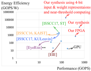
Figure 15. Comparison on performance and energy efficiency with state-of-the-art ASIC results.

In Fig. 15, we can observe that our synthesis results achieve both the highest throughput and energy efficiency, more than 6 times compared with the highest energy efficiency in the best state-of-the-art implementations. It is also striking that even our FPGA implementation could achieve the same order of energy efficiency and higher throughput compared with the best state-of-the-art ASICs. It is worth noting that the best state-of-the-art ASIC implementations report the highest energy efficiency in the near-threshold regime with an aggressively reduced bit-length (say 4 bits, with a significant accuracy reduction in this case). When using 4-bit input and weight representations and near-threshold computing of 0.55V $V_{dd}$ voltage level, another 17$\times$ improvement on energy efficiency can be achieved in the synthesis results compared with our super-threshold implementation, as shown in Fig. 15. This makes it a total of 102$\times$ improvement compared with the best state-of-the-art. Moreover, in our systems (in the super-threshold implementation), memory in fact consumes slightly less power consumption compared with computing blocks, which demonstrates that weight storage is no longer the system bottleneck. Please note that the overall accuracy when using 4-bit representation is low in CirCNN architecture (e.g., less than 20% for AlexNet). Hence, 4-bit representation is only utilized to provide a fair comparison with the baseline methods using the same number of bits for representations.

We also perform comparison on performance and energy efficiency with the most energy-efficient NVIDIA Jetson TX1 embedded GPU toolkit, which is optimized for deep learning applications. It can be observed that an energy efficiency improvement of 570$\times$ can be achieved using our implementation, and the improvement reaches 9,690$\times$ when incorporating near-threshold computing and 4-bit weight and input representations.

5.3. Embedded ARM-based Processors

Because ARM-based embedded processors are the most widely used embedded processors in smartphones, embedded and IoT devices, we implement the proposed block-circulant matrix-based DNN inference framework on a smartphone using ARM Cortex A9 processor cores, and provide some sample results. The aim is to demonstrate the potential of real-time implementation of deep learning systems on embedded processors, thereby significantly enhancing the wide adoption of (large-scale) deep learning systems in personal, embedded, and IoT devices. In the implementation of LeNet-5 DCNN model on the MNIST data set, the proposed embedded processor-based implementation achieves a performance of 0.9ms/image with 96% accuracy, which is slightly faster compared with IBM TrueNorth in the high-accuracy mode (esser2015backpropagation, ) (1000 Images/s). The energy efficiency is slightly lower but at the same level due to the peripheral devices in a smartphone. When comparing with a GPU-based implementation using NVIDIA Tesla C2075 GPU with 2,333 Images/s, the energy efficiency is significantly higher because the GPU consumes 202.5W power consumption, while the embedded processor only consumes around 1W. It is very interesting that when comparing on the fully-connected layer of AlexNet, our smartphone-based implementation of CirCNN even achieves higher throughput (667 Layers/s vs. 573 Layers/s) compared with NVIDIA Tesla GPU. This is because the benefits of computational complexity reduction become more significant when the model size becomes larger.

5.4. Summary and Discussions

Energy Efficiency and Performance: Overall, CirCNN architecture achieves a significant gain in energy efficiency and performance compared with the best state-of-the-arts on different platforms including FPGAs, ASIC designs, and embedded processors. The key reasons of such improvements include the fundamental algorithmic improvements, weight storage reduction, a significant reduction of off-chip DRAM accessing, and the highly efficient implementation of the basic computing block for FFT/IFFT calculations. The fundamental algorithmic improvements accounts for the most significant portion of energy efficiency and performance improvements around 10$\times$-20$\times$, and the rest accounts for 2$\times$-5$\times$. In particular, we emphasize that: 1) the hardware resources and power/energy consumptions associated with memory storage will be at the same order as the computing blocks and will not be the absolute dominating factor of the overall hardware deep learning system; 2) medium to large-scale DNN models can be implemented in small footprint thanks to the recursive property of FFT/IFFT calculations. These characteristics are the key to enable highly efficient implementations of CirCNN architecture in low-power FPGAs/ASICs and the elimination of complex control logics and high-power-consumption clock networks.

Reconfigurability: It is a key property of CirCNN architecture, allowing it be applied to a wide set of deep learning systems. It resembles IBM TrueNorth and could significantly reduce the development round and promote the wide application of deep learning systems. Unlike IBM TrueNorth, CirCNN1) does not need a specialized offline training framework and specific preprocessing procedures for certain data sets like CIFAR (esser2016convolutional, ); and 2) does not result in any hardware resource waste for small-scale neural networks and additional chips for large-scale ones. The former property is because the proposed training algorithms are general, and the latter is because different scales of DNN models can be conducted on the same basic computing block using different control signals thanks to the recursive property of FFT/IFFT. The software interface of reconfigurability is under development and will be released for public testing.

Online Learning Capability: The CirCNN architecture described mainly focuses on the inference process of deep learning systems, although its algorithmic framework applies to both inference and training. We focus on inference because it is difficult to perform online training in hardware embedded deep learning systems due to the limited computing power and data set they can encounter.

6. Conclusion

This paper proposes CirCNN, a principled approach to represent weights and process neural networks using block-circulant matrices. CirCNN utilizes the Fast Fourier Transform (FFT)-based fast multiplication, simultaneously reducing the computational complexity (both in inference and training) from O($n^{2}$) to O($n\log n$) and the storage complexity from O($n^{2}$) to O($n$), with negligible accuracy loss. We propose the CirCNN architecture, a universal DNN inference engine that can be implemented in various hardware/software platforms with configurable network architecture (e.g., layer type, size, scales, etc.). To demonstrate the performance and energy efficiency, we test CirCNN architecture in FPGA, ASIC and embedded processors. Our results show that CirCNN architecture achieves very high energy efficiency and performance with a small hardware footprint. Based on the FPGA implementation and ASIC synthesis results, CirCNN achieves 6 - 102$\times$ energy efficiency improvements compared with the best state-of-the-art results.

7. Acknowledgement

This work is funded by the National Science Foundation Awards CNS-1739748, CNS-1704662, CNS-1337300, CRII-1657333, CCF-1717754, CNS-1717984, Algorithm-in-the-Field program, DARPA SAGA program, and CASE Center at Syracuse University.

References

- (1) J. Deng, W. Dong, R. Socher, L.-J. Li, K. Li, and L. Fei-Fei, “Imagenet: A large-scale hierarchical image database,” in Computer Vision and Pattern Recognition, 2009. CVPR 2009. IEEE Conference on, pp. 248–255, IEEE, 2009.
- (2) Y. Taigman, M. Yang, M. Ranzato, and L. Wolf, “Deepface: Closing the gap to human-level performance in face verification,” in Proceedings of the IEEE Conference on Computer Vision and Pattern Recognition, pp. 1701–1708, 2014.
- (3) B. Huval, T. Wang, S. Tandon, J. Kiske, W. Song, J. Pazhayampallil, M. Andriluka, P. Rajpurkar, T. Migimatsu, R. Cheng-Yue, et al., “An empirical evaluation of deep learning on highway driving,” arXiv preprint arXiv:1504.01716, 2015.
- (4) R. Collobert and J. Weston, “A unified architecture for natural language processing: Deep neural networks with multitask learning,” in Proceedings of the 25th international conference on Machine learning, pp. 160–167, ACM, 2008.
- (5) R. Burbidge, M. Trotter, B. Buxton, and S. Holden, “Drug design by machine learning: support vector machines for pharmaceutical data analysis,” Computers & chemistry, vol. 26, no. 1, pp. 5–14, 2001.
- (6) A. Krizhevsky, I. Sutskever, and G. E. Hinton, “Imagenet classification with deep convolutional neural networks,” in Advances in neural information processing systems, pp. 1097–1105, 2012.
- (7) A. Karpathy and L. Fei-Fei, “Deep visual-semantic alignments for generating image descriptions,” in Proceedings of the IEEE Conference on Computer Vision and Pattern Recognition, pp. 3128–3137, 2015.
- (8) B. Catanzaro, “Deep learning with cots hpc systems,” 2013.
- (9) K. Simonyan and A. Zisserman, “Very deep convolutional networks for large-scale image recognition,” arXiv preprint arXiv:1409.1556, 2014.
- (10) Q. V. Le, “Building high-level features using large scale unsupervised learning,” in Acoustics, Speech and Signal Processing (ICASSP), 2013 IEEE International Conference on, pp. 8595–8598, IEEE, 2013.
- (11) D. Ciregan, U. Meier, and J. Schmidhuber, “Multi-column deep neural networks for image classification,” in Computer Vision and Pattern Recognition (CVPR), 2012 IEEE Conference on, pp. 3642–3649, IEEE, 2012.
- (12) J. Schmidhuber, “Deep learning in neural networks: An overview,” Neural networks, vol. 61, pp. 85–117, 2015.
- (13) N. Suda, V. Chandra, G. Dasika, A. Mohanty, Y. Ma, S. Vrudhula, J.-s. Seo, and Y. Cao, “Throughput-optimized opencl-based fpga accelerator for large-scale convolutional neural networks,” in Proceedings of the 2016 ACM/SIGDA International Symposium on Field-Programmable Gate Arrays, pp. 16–25, ACM, 2016.
- (14) J. Qiu, J. Wang, S. Yao, K. Guo, B. Li, E. Zhou, J. Yu, T. Tang, N. Xu, S. Song, et al., “Going deeper with embedded fpga platform for convolutional neural network,” in Proceedings of the 2016 ACM/SIGDA International Symposium on Field-Programmable Gate Arrays, pp. 26–35, ACM, 2016.
- (15) C. Zhang, Z. Fang, P. Zhou, P. Pan, and J. Cong, “Caffeine: towards uniformed representation and acceleration for deep convolutional neural networks,” in Proceedings of the 35th International Conference on Computer-Aided Design, p. 12, ACM, 2016.
- (16) C. Zhang, D. Wu, J. Sun, G. Sun, G. Luo, and J. Cong, “Energy-efficient cnn implementation on a deeply pipelined fpga cluster,” in Proceedings of the 2016 International Symposium on Low Power Electronics and Design, pp. 326–331, ACM, 2016.
- (17) D. Mahajan, J. Park, E. Amaro, H. Sharma, A. Yazdanbakhsh, J. K. Kim, and H. Esmaeilzadeh, “Tabla: A unified template-based framework for accelerating statistical machine learning,” in High Performance Computer Architecture (HPCA), 2016 IEEE International Symposium on, pp. 14–26, IEEE, 2016.
- (18) R. Zhao, W. Song, W. Zhang, T. Xing, J.-H. Lin, M. Srivastava, R. Gupta, and Z. Zhang, “Accelerating binarized convolutional neural networks with software-programmable fpgas,” in Proceedings of the 2017 ACM/SIGDA International Symposium on Field-Programmable Gate Arrays, pp. 15–24, ACM, 2017.
- (19) Y. Umuroglu, N. J. Fraser, G. Gambardella, M. Blott, P. Leong, M. Jahre, and K. Vissers, “Finn: A framework for fast, scalable binarized neural network inference,” in Proceedings of the 2017 ACM/SIGDA International Symposium on Field-Programmable Gate Arrays, pp. 65–74, ACM, 2017.
- (20) S. Han, J. Kang, H. Mao, Y. Hu, X. Li, Y. Li, D. Xie, H. Luo, S. Yao, Y. Wang, et al., “Ese: Efficient speech recognition engine with sparse lstm on fpga,” in Proceedings of the 2017 ACM/SIGDA International Symposium on Field-Programmable Gate Arrays, pp. 75–84, ACM, 2017.
- (21) http://www.techradar.com/news/computing-components/processors/google-s-tensor-processing-unit-explained-this-is-what-the-future-of- computing-looks-like-1326915.
- (22) https://www.sdxcentral.com/articles/news/intels-deep-learning-chips-will-arrive-2017/2016/11/.
- (23) Y.-H. Chen, T. Krishna, J. S. Emer, and V. Sze, “Eyeriss: An energy-efficient reconfigurable accelerator for deep convolutional neural networks,” IEEE Journal of Solid-State Circuits, vol. 52, no. 1, pp. 127–138, 2017.
- (24) S. Han, X. Liu, H. Mao, J. Pu, A. Pedram, M. A. Horowitz, and W. J. Dally, “Eie: efficient inference engine on compressed deep neural network,” in Proceedings of the 43rd International Symposium on Computer Architecture, pp. 243–254, IEEE Press, 2016.
- (25) T. Chen, Z. Du, N. Sun, J. Wang, C. Wu, Y. Chen, and O. Temam, “Diannao: A small-footprint high-throughput accelerator for ubiquitous machine-learning,” in ACM Sigplan Notices, vol. 49, pp. 269–284, ACM, 2014.
- (26) Y. Chen, T. Luo, S. Liu, S. Zhang, L. He, J. Wang, L. Li, T. Chen, Z. Xu, N. Sun, et al., “Dadiannao: A machine-learning supercomputer,” in Proceedings of the 47th Annual IEEE/ACM International Symposium on Microarchitecture, pp. 609–622, IEEE Computer Society, 2014.
- (27) Z. Du, R. Fasthuber, T. Chen, P. Ienne, L. Li, T. Luo, X. Feng, Y. Chen, and O. Temam, “Shidiannao: Shifting vision processing closer to the sensor,” in ACM SIGARCH Computer Architecture News, vol. 43, pp. 92–104, ACM, 2015.
- (28) B. Reagen, P. Whatmough, R. Adolf, S. Rama, H. Lee, S. K. Lee, J. M. Hernández-Lobato, G.-Y. Wei, and D. Brooks, “Minerva: Enabling low-power, highly-accurate deep neural network accelerators,” in Proceedings of the 43rd International Symposium on Computer Architecture, pp. 267–278, IEEE Press, 2016.
- (29) G. Desoli, N. Chawla, T. Boesch, S.-p. Singh, E. Guidetti, F. De Ambroggi, T. Majo, P. Zambotti, M. Ayodhyawasi, H. Singh, et al., “14.1 a 2.9 tops/w deep convolutional neural network soc in fd-soi 28nm for intelligent embedded systems,” in Solid-State Circuits Conference (ISSCC), 2017 IEEE International, pp. 238–239, IEEE, 2017.
- (30) B. Moons, R. Uytterhoeven, W. Dehaene, and M. Verhelst, “14.5 envision: A 0.26-to-10tops/w subword-parallel dynamic-voltage-accuracy-frequency-scalable convolutional neural network processor in 28nm fdsoi,” in Solid-State Circuits Conference (ISSCC), 2017 IEEE International, pp. 246–247, IEEE, 2017.
- (31) J. Sim, J. Park, M. Kim, D. Bae, Y. Choi, and L. Kim, “A 1.42 tops/w deep convolutional neural network recognition processor for intelligent iot systems,” in 2016 IEEE ISSCC, IEEE solid-state circuits society, 2016.
- (32) P. N. Whatmough, S. K. Lee, H. Lee, S. Rama, D. Brooks, and G.-Y. Wei, “14.3 a 28nm soc with a 1.2 ghz 568nj/prediction sparse deep-neural-network engine with¿ 0.1 timing error rate tolerance for iot applications,” in Solid-State Circuits Conference (ISSCC), 2017 IEEE International, pp. 242–243, IEEE, 2017.
- (33) S. Bang, J. Wang, Z. Li, C. Gao, Y. Kim, Q. Dong, Y.-P. Chen, L. Fick, X. Sun, R. Dreslinski, et al., “14.7 a 288w programmable deep-learning processor with 270kb on-chip weight storage using non-uniform memory hierarchy for mobile intelligence,” in Solid-State Circuits Conference (ISSCC), 2017 IEEE International, pp. 250–251, IEEE, 2017.
- (34) S. Han, J. Pool, J. Tran, and W. Dally, “Learning both weights and connections for efficient neural network,” in Advances in Neural Information Processing Systems, pp. 1135–1143, 2015.
- (35) S. Han, H. Mao, and W. J. Dally, “Deep compression: Compressing deep neural networks with pruning, trained quantization and huffman coding,” arXiv preprint arXiv:1510.00149, 2015.
- (36) J. Wu, C. Leng, Y. Wang, Q. Hu, and J. Chen, “Quantized convolutional neural networks for mobile devices,” in Computer Vision and Pattern Recognition, 2016. CVPR 2016. IEEE Conference on, 2016.
- (37) D. Lin, S. Talathi, and S. Annapureddy, “Fixed point quantization of deep convolutional networks,” in International Conference on Machine Learning, pp. 2849–2858, 2016.
- (38) M. Jaderberg, A. Vedaldi, and A. Zisserman, “Speeding up convolutional neural networks with low rank expansions,” arXiv preprint arXiv:1405.3866, 2014.
- (39) C. Tai, T. Xiao, Y. Zhang, X. Wang, et al., “Convolutional neural networks with low-rank regularization,” arXiv preprint arXiv:1511.06067, 2015.
- (40) J. Yu, A. Lukefahr, D. Palframan, G. Dasika, R. Das, and S. Mahlke, “Scalpel: Customizing dnn pruning to the underlying hardware parallelism,” in Proceedings of the 44th Annual International Symposium on Computer Architecture, pp. 548–560, ACM, 2017.
- (41) V. Pan, Structured matrices and polynomials: unified superfast algorithms. Springer Science & Business Media, 2012.
- (42) https://drive.google.com/open?id=0B19Xkz1gXlwAYjVjWC1Kc2xSRm8.
- (43) L. Zhao, S. Liao, Y. Wang, J. Tang, and B. Yuan, “Theoretical properties for neural networks with weight matrices of low displacement rank,” arXiv preprint arXiv:1703.00144, 2017.
- (44) H. Lee, R. Grosse, R. Ranganath, and A. Y. Ng, “Convolutional deep belief networks for scalable unsupervised learning of hierarchical representations,” in Proceedings of the 26th annual international conference on machine learning, pp. 609–616, ACM, 2009.
- (45) A. Karpathy, G. Toderici, S. Shetty, T. Leung, R. Sukthankar, and L. Fei-Fei, “Large-scale video classification with convolutional neural networks,” in Proceedings of the IEEE conference on Computer Vision and Pattern Recognition, pp. 1725–1732, 2014.
- (46) D. Yu and L. Deng, “Deep learning and its applications to signal and information processing [exploratory dsp],” IEEE Signal Processing Magazine, vol. 28, no. 1, pp. 145–154, 2011.
- (47) Y. LeCun, L. Bottou, Y. Bengio, and P. Haffner, “Gradient-based learning applied to document recognition,” Proceedings of the IEEE, vol. 86, no. 11, pp. 2278–2324, 1998.
- (48) J. Xue, J. Li, and Y. Gong, “Restructuring of deep neural network acoustic models with singular value decomposition.,” in Interspeech, pp. 2365–2369, 2013.
- (49) B. Liu, W. Wen, Y. Chen, X. Li, C.-R. Wu, and T.-Y. Ho, “Eda challenges for memristor-crossbar based neuromorphic computing,” in Proceedings of the 25th edition on Great Lakes Symposium on VLSI, pp. 185–188, ACM, 2015.
- (50) J. Chung and T. Shin, “Simplifying deep neural networks for neuromorphic architectures,” in Design Automation Conference (DAC), 2016 53nd ACM/EDAC/IEEE, pp. 1–6, IEEE, 2016.
- (51) K. Hwang and W. Sung, “Fixed-point feedforward deep neural network design using weights+ 1, 0, and- 1,” in Signal Processing Systems (SiPS), 2014 IEEE Workshop on, pp. 1–6, IEEE, 2014.
- (52) M. Mathieu, M. Henaff, and Y. LeCun, “Fast training of convolutional networks through ffts,” arXiv preprint arXiv:1312.5851, 2013.
- (53) K. He, X. Zhang, S. Ren, and J. Sun, “Deep residual learning for image recognition,” in Proceedings of the IEEE Conference on Computer Vision and Pattern Recognition, pp. 770–778, 2016.
- (54) Y. Cheng, F. X. Yu, R. S. Feris, S. Kumar, A. Choudhary, and S.-F. Chang, “An exploration of parameter redundancy in deep networks with circulant projections,” in Proceedings of the IEEE International Conference on Computer Vision, pp. 2857–2865, 2015.
- (55) D. Bini, V. Pan, and W. Eberly, “Polynomial and matrix computations volume 1: Fundamental algorithms,” SIAM Review, vol. 38, no. 1, pp. 161–164, 1996.
- (56) Y. Jia, E. Shelhamer, J. Donahue, S. Karayev, J. Long, R. Girshick, S. Guadarrama, and T. Darrell, “Caffe: Convolutional architecture for fast feature embedding,” in Proceedings of the 22nd ACM international conference on Multimedia, pp. 675–678, ACM, 2014.
- (57) A. Vedaldi and K. Lenc, “Matconvnet: Convolutional neural networks for matlab,” in Proceedings of the 23rd ACM international conference on Multimedia, pp. 689–692, ACM, 2015.
- (58) L. Narici and E. Beckenstein, “The hahn-banach theorem: the life and times,” Topology and its Applications, vol. 77, no. 2, pp. 193–211, 1997.
- (59) Y. Netzer, T. Wang, A. Coates, A. Bissacco, B. Wu, and A. Y. Ng, “Reading digits in natural images with unsupervised feature learning,” in NIPS workshop on deep learning and unsupervised feature learning, vol. 2011, p. 5, 2011.
- (60) A. Krizhevsky and G. Hinton, “Learning multiple layers of features from tiny images,” 2009.
- (61) A. Coates, H. Lee, and A. Y. Ng, “An analysis of single-layer networks in unsupervised feature learning,” Ann Arbor, vol. 1001, no. 48109, p. 2, 2010.
- (62) L. Deng, “The mnist database of handwritten digit images for machine learning research [best of the web],” IEEE Signal Processing Magazine, vol. 29, no. 6, pp. 141–142, 2012.
- (63) S. A. Salehi, R. Amirfattahi, and K. K. Parhi, “Pipelined architectures for real-valued fft and hermitian-symmetric ifft with real datapaths,” IEEE Transactions on Circuits and Systems II: Express Briefs, vol. 60, no. 8, pp. 507–511, 2013.
- (64) Y.-N. Chang and K. K. Parhi, “An efficient pipelined fft architecture,” IEEE Transactions on Circuits and Systems II: Analog and Digital Signal Processing, vol. 50, no. 6, pp. 322–325, 2003.
- (65) C. Cheng and K. K. Parhi, “High-throughput vlsi architecture for fft computation,” IEEE Transactions on Circuits and Systems II: Express Briefs, vol. 54, no. 10, pp. 863–867, 2007.
- (66) M. Garrido, K. K. Parhi, and J. Grajal, “A pipelined fft architecture for real-valued signals,” IEEE Transactions on Circuits and Systems I: Regular Papers, vol. 56, no. 12, pp. 2634–2643, 2009.
- (67) M. Ayinala, Y. Lao, and K. K. Parhi, “An in-place fft architecture for real-valued signals,” IEEE Transactions on Circuits and Systems II: Express Briefs, vol. 60, no. 10, pp. 652–656, 2013.
- (68) M. Ayinala and K. K. Parhi, “Fft architectures for real-valued signals based on radix-$2{̂3}$ and radix-$2{̂4}$ algorithms,” IEEE Transactions on Circuits and Systems I: Regular Papers, vol. 60, no. 9, pp. 2422–2430, 2013.
- (69) A. V. Oppenheim, Discrete-time signal processing. Pearson Education India, 1999.
- (70) Altera, “Fft mega-core function user guide,” Altera, San Jose, Calif, USA, 2010.
- (71) P. Judd, J. Albericio, T. Hetherington, T. M. Aamodt, and A. Moshovos, “Stripes: Bit-serial deep neural network computing,” in Microarchitecture (MICRO), 2016 49th Annual IEEE/ACM International Symposium on, pp. 1–12, IEEE, 2016.
- (72) https://www.altera.com/products/fpga/stratix-series/stratix-10/overview.html.
- (73) https://www.xilinx.com/products/silicon-devices/fpga/virtex-7.html.
- (74) W. Wang, P. Mishra, and S. Ranka, “Dynamic cache reconfiguration and partitioning for energy optimization in real-time multi-core systems,” in Proceedings of the 48th Design Automation Conference, pp. 948–953, ACM, 2011.
- (75) A. Gordon-Ross, J. Lau, and B. Calder, “Phase-based cache reconfiguration for a highly-configurable two-level cache hierarchy,” in Proceedings of the 18th ACM Great Lakes symposium on VLSI, pp. 379–382, ACM, 2008.
- (76) N. P. Jouppi, “Improving direct-mapped cache performance by the addition of a small fully-associative cache prefetch buffers,” in 25 years of the international symposia on Computer architecture (selected papers), pp. 388–397, ACM, 1998.
- (77) J. Dundas and T. Mudge, “Improving data cache performance by pre-executing instructions under a cache miss,” in Proceedings of the 11th international conference on Supercomputing, pp. 68–75, ACM, 1997.
- (78) N. Weste, D. Harris, and A. Banerjee, “Cmos vlsi design,” A circuits and systems perspective, vol. 11, p. 739, 2005.
- (79) S. K. Esser, P. A. Merolla, J. V. Arthur, A. S. Cassidy, R. Appuswamy, A. Andreopoulos, D. J. Berg, J. L. McKinstry, T. Melano, D. R. Barch, et al., “Convolutional networks for fast, energy-efficient neuromorphic computing,” Proceedings of the National Academy of Sciences, p. 201604850, 2016.
- (80) S. K. Esser, R. Appuswamy, P. Merolla, J. V. Arthur, and D. S. Modha, “Backpropagation for energy-efficient neuromorphic computing,” in Advances in Neural Information Processing Systems, pp. 1117–1125, 2015.
- (81) http://www.nangate.com/?page_id=22.
- (82) http://quid.hpl.hp.com:9081/cacti/.