Testing for polytomies in phylogenetic species trees using quartet frequencies

Abstract

Phylogenetic species trees typically represent the speciation history as a bifurcating tree. Speciation events that simultaneously create more than two descendants, thereby creating polytomies in the phylogeny, are possible. Moreover, the inability to resolve relationships is often shown as a (soft) polytomy. Both types of polytomies have been traditionally studied in the context of gene tree reconstruction from sequence data. However, polytomies in the species tree cannot be detected or ruled out without considering gene tree discordance. In this paper, we describe a statistical test based on properties of the multi-species coalescent model to test the null hypothesis that a branch in an estimated species tree should be replaced by a polytomy. On both simulated and biological datasets, we show that the null hypothesis is rejected for all but the shortest branches, and in most cases, it is retained for true polytomies. The test, available as part of the ASTRAL package, can help systematists decide whether their datasets are sufficient to resolve specific relationships of interest.

Index terms— Incomplete Lineage Sorting, Multi-species Coalescent Model, Summary Methods, Phylogenomics, Polytomy, Multifurcation, Statistical Test

1 Introduction

Phylogenies are typically modeled as bifurcating trees. Even when the evolution is fully vertical, which it is not always Bapteste et al. (2013); Nakhleh (2011), the binary model precludes the possibility of several species evolving simultaneously from a progenitor species Hoelzer and Meinick (1994). These events could be modeled in a multifurcating tree where some nodes, called polytomies, have more than two children. True polytomies have been suggested for several parts of the tree-of-life (e.g., Suh (2016); Arntzen et al. (2007)). Polytomies are also used when the analyst is unsure about some relationships due to a lack of signal in the data to resolve relationships Townsend et al. (2012). The terms hard and soft polytomies are used to distinguish between these two cases Maddison (1989), with a soft polytomy reserved for the case where relationships are unresolved in an estimated tree and a hard polytomy for multifurcations in the true tree (Fig. 1). Distinguishing the two types of polytomies is not easy. Moreover, the distinction between soft and hard polytomies can be blurred. The difficulty in resolving relationships increases as branches become shorter. In the limit, a branch of length zero is equivalent to a hard polytomy, which is not just difficult but impossible to resolve. Regardless of abstract distinctions, a major difficulty faced by systematists is to detect whether specific resolutions in their inferred trees are sufficiently supported by data to rule out a polytomy (e.g., see Chojnowski et al. (2008); Suh (2016)).

For any branch of a given species tree, we can pose a null hypothesis that the length of that branch is zero, and thus, the branch should be removed to create a polytomy. Using observed data, we can try to reject this null hypothesis, and if we fail to reject, we can replace the branch with a polytomy. The resulting polytomy is best understood as a soft polytomy because the inability to reject a null hypothesis is never accepting the alternative hypothesis. The inability to reject may be caused by a real (i.e., hard) polytomy, but it may also simply be due to the lack of power (Fig. 1). In this paper, we present a new test with polytomy as the null hypothesis for multi-locus datasets.

The idea of testing a polytomy as the null hypothesis and rejecting it using data has been applied to single-locus data Jackman et al. (1999); Walsh et al. (1999). Likelihood ratio tests against a zero-length branch have been developed (e.g., SOWH test Swofford et al. (1996)) and are implemented in popular packages such as PAUP* Swofford (2003). Treating polytomies as the null hypothesis has been pioneered by Walsh et al. who sought to not only test for polytomies but also to use a power analysis to distinguish soft and hard polytomies Walsh et al. (1999). Appraising their general framework, Braun and Kimball Braun and Kimball (2001) showed that the power analysis can be sensitive to model complexity (or lack thereof). Perhaps most relevant to our work, Anisimova et al. presented an approximate but fast likelihood ratio test for a polytomy null hypothesis Anisimova et al. (2006); their test, like what we will present looks at each branch and its surrounding branches while ignoring the rest of the tree.

The existing tests of polytomy as the null and also Bayesian methods of modeling polytomies Lewis et al. (2005) assume that the sequence data follow a single tree. Therefore, these methods test whether a gene tree includes a polytomy Slowinski (2001). However, the species tree can be different from gene trees and the discordance can have several causes, including gene duplication and loss, lateral gene transfer, and incomplete lineage sorting Degnan and Rosenberg (2009); Maddison (1997). Arguably, the question of interest is whether the species tree includes polytomies. Moreover, we are often interested to know whether we should treat the relationship between species as unresolved given the amount of data at hand. These questions cannot be answered without considering gene tree discordance, an observation made previously by others as well Slowinski (2001); Poe and Chubb (2004). For example, Poe and Chubb Poe and Chubb (2004), in analyzing an avian dataset with five genes, first looked for zero-length branches in the gene trees using the SOWH test Swofford et al. (1996) and found evidence that some gene trees may include polytomies. But they also tested if the pairwise similarity between gene trees was greater than a set of random trees and it was not. Their test of gene tree congruence, however, was not with respect to any particular model of gene tree evolution.

A major cause of gene tree discordance is a population-level process called incomplete lineage sorting (ILS), which has been modeled by the multi-species coalescent (MSC) model Rannala and Yang (2003); Pamilo and Nei (1988). The model tells us that that likelihood of ILS causing discordance increases as branches become shorter; therefore, any test of polytomies should also consider ILS. The MSC model has been extensively used for reconstructing species trees using many approaches, including Bayesian co-estimation of gene trees and species trees Heled and Drummond (2010); Liu (2008) and site-based approaches Chifman and Kubatko (2014); Bryant et al. (2012). A popular approach (due to its scalability) is the summary method, where we first reconstruct gene trees individually and then summarize them to build the species tree. Many approaches that model ILS rely on dividing the dataset into quartets of species. These quartet-based methods (e.g., the summary method ASTRAL Mirarab et al. (2014); Mirarab and Warnow (2015); Zhang et al. (2017), the site-based method SVDQuartets Chifman and Kubatko (2014), and a hybrid method called Bucky-Quartet Larget et al. (2010)) rely on the fact that for a quartet of species, where only three unrooted tree topologies are possible, the species tree topology has the highest probability of occurring in unrooted gene trees under the MSC model (Fig. 1a).

Relying on the known distribution of quartet frequencies under the MSC model, we previously introduced a way of computing the support of a branch using a measure called local posterior probability (localPP) Sayyari and Mirarab (2016). In this paper, we further extend the approach used to compute localPP to develop a fast test for the null hypothesis that a branch has length zero. Under the null hypothesis, we expect that the three unrooted quartet topologies defined around the branch should have equal frequencies Allman et al. (2011). This can be rigorously tested, resulting in the approach we present. Similar ideas have been mentioned in passing previously by Slowinski Slowinski (2001) and by Allman et al. Allman et al. (2011) but to our knowledge, these suggestions have never been implemented or tested. The statistical test that we present is implemented inside the ASTRAL package (option -t 10) since version 4.11.2 and is available online at https://github.com/smirarab/ASTRAL.

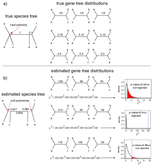
Figure 1: A statistical test of polytomies. (a) We show an example true species tree with a hard polytomy and two branches with CU lengths 1 and 0.1 (left), and the expected quartet gene tree fractions for three selected quartets based on the MSC model (right). The first quartet is around a true (hard) polytomy and has $\frac{1}{3}$ fraction expected for all three alternative topologies. (b) An estimated species tree with estimated CU branch lengths (left) and a hypothetical set of quartet tree frequencies counted from 300 hypothetical gene trees (right). Below each set of quartets, we show the computation of the $\chi^{2}$ test statistic, and show where it falls on the $\chi^{2}$ distribution with $DF=2$; the vertical blue line shows the computed $\chi^{2}$ based on given counts and the shaded red areas inside distributions show the area under the $\chi^{2}$ distribution corresponding to the $p$-value. The null hypothesis is not rejected for the branch corresponding to the true polytomy (a true negative) or the short 0.1 CU branch (a false negative); these branches (dotted lines in the species tree) can be replaced with soft polytomies.

2 Materials and Methods

2.1 Background

An unrooted tree defined on a quartet of species $\{a,b,c,d\}$ can have one of three topologies (Fig. 1a): $t_{1}=ab\|cd$ (i.e., $a$ and $b$ are closer to each other than $c$, and $d$), $t_{2}=ac\|bd$, or $t_{3}=ad\|bc$. Consider an unrooted species tree $ab\|cd$ where the internal branch length separating species $a$ and $b$ from $c$ and $d$ is $x$ in coalescent units (CU), which is the number of generations divided by the haploid population size Degnan and Rosenberg (2009). Under the Multi Species Coalescent (MSC) model, each gene tree matches the species tree with the probability $p_{1}=1-\frac{2}{3}e^{-x}$ and matches each of the two alternative topologies with the probability $p_{2}=p_{3}=\frac{1}{3}e^{-x}$ (Allman et al., 2011). Given true (i.e., error-free) gene trees with no recombination within a locus but free recombination across loci, frequencies $n_{1},n_{2},n_{3}$ of gene trees matching topologies $t_{1},t_{2},t_{3}$ will follow a multinomial distribution with parameters $p_{1},p_{2},p_{3}$ and with the number of trials equal $n=n_{1}+n_{2}+n_{3}$. Clearly, for a species tree with $N>4$ species, the same results are applicable for any of the ${N\choose 4}$ selections of a quartet of the species with $x$ defined to be the branch length on the species tree restricted to the quartet (see Fig. 1 for examples).

2.2 A statistical test of polytomy

A true polytomy is mathematically identical to a bifurcating node that has at least one adjacent branch with length zero; the zero-length branch can be contracted in the binary tree to introduce the polytomy (e.g., compare branches P4 – P6 in Fig. 2a to the multifurcating tree), If the true species tree for a quartet of taxa has a polytomy (i.e., $x=0$), then all gene tree topologies are equally likely with $p_{1}=p_{2}=p_{3}=\frac{1}{3}$. Thus, if we had the true $p_{i}$ values, we would immediately know if the species tree has a polytomy. However, we can never know true $p_{i}$ parameters; instead, we have observations $n_{1},n_{2},n_{3}$ with $\operatorname{\mathbb{E}}(n_{i})/n=p_{i}$. Luckily, multinomial distributions concentrate around their mean. As the number of genes increases, the probability of quartet frequencies deviating from their mean rapidly drops; for example, according to Hoeffding’s inequality, the probability of divergence by $\epsilon$ drops exponentially and is no more than $2e^{-2\epsilon^{2}n}$. This concentration gives us hope that even though we never know true $p_{i}$ values from limited data, we can design statistical tests for a $p=\frac{1}{3}$ null hypothesis. For an internal branch $\mathcal{B}$ in a bifurcating species tree, consider the following.

Null hypothesis:

The length of the internal branch $\mathcal{B}$ is zero; thus, the species tree has a polytomy.

To test this null hypothesis, we can use quartet gene tree frequencies given three assumptions.

1. All positive length branches in the given species tree are correct.

2. Gene trees are a random error-free sample from the distribution defined by the MSC model.

3. We have $n\geq 10$ gene trees with at least a quartet relevant to $\mathcal{B}$.

A1, which we have previously called the locality assumption Sayyari and Mirarab (2016), can be somewhat relaxed. For each bipartition (i.e., branch) of the true species tree, either that bipartition or one of its NNI rearrangements should be present in the given species tree.

We now describe expectations under the null hypothesis. With start with the $N=4$ case. By the A2 assumption, frequencies $n_{1},n_{2},n_{3}$ follow a multinomial distribution with parameters $(p_{1},p_{2},p_{3},n)$. Under the null hypothesis $p_{1}=p_{2}=p_{3}=\frac{1}{3}$. Thus,under the null,

$$\chi^{2}=\frac{(n_{1}-n/3)^{2}}{n/3}+\frac{(n_{2}-n/3)^{2}}{n/3}+\frac{(n_{3}-n/3)^{2}}{n/3}$$ (1)

is asymptotically a chi-squared random variable with 2 degrees of freedom (Zar, 2007). This chi-squared approximation for three equiprobable outcomes is a good approximation when $n\geq 10$ (Koehler and Larntz, 1980; Zar, 2007; Read and Cressie, 1988), hence our assumption A3. For smaller $n$’s an exact calculation of the critical value is required (Read and Cressie, 1988), but we simply avoid applying our test for $n<10$. Given the chi-squared random variable as the test statistic, we can simply use a Pearson’s goodness-of-fit statistical test. Thus, the $p$-value is the area to the right of the $\chi^{2}$ test statistic (Eq. 1) under the probability density function of the chi-square distribution with two degrees of freedom (Fig. 1b). This integral is available in various software packages, including the Java package colt Hoschek (2004), which we use.

With $N>4$, we apply the test described above to each branch of the species tree independently. For each branch $\mathcal{B}$, we will have multiple quartets around that branch. We say that a quartet of species $\{a,b,c,d\}$ is around the branch $\mathcal{B}$ when it is chosen as follows: select an arbitrary leaf $a$ from the subtree under the left child of $\mathcal{B}$, $b$ from the subtree under the right child of $\mathcal{B}$, $c$ from the subtree under the sister branch of $\mathcal{B}$, and $d$ from the subtree under the sister branch of the parent of $\mathcal{B}$ (this can be easily adopted for a branch incident to root). Note that by assumption A1 (and its relaxed version), the length of the internal branch of the unrooted species tree induced down to a quartet around $\mathcal{B}$ is identical to the length of $\mathcal{B}$. Thus, under the null hypothesis, for any quartet around $\mathcal{B}$, we expect that the length of the quartet branch should be zero. Thus, any arbitrary selection of a quartet around the branch would enable us to use the same exact test we described before for $N=4$.

Following the approach we previously used for defining localPP Sayyari and Mirarab (2016), we can also use all quartets around the branch. More precisely, let $n_{i,j}$ for $1\leq i\leq 3,1\leq j\leq n$ be the number of quartets around the branch $\mathcal{B}$ that in gene tree $j$ have the topology $t_{i}$ and let $f_{i,j}=\frac{n_{i,j}}{n_{1,j}+n_{2,j}+n_{3,j}}$. Then, we define

$$n_{i}=\sum_{j=1}^{n}f_{i,j}=\sum_{j=1}^{n}\frac{n_{i,j}}{n_{1,j}+n_{2,j}+n_{3,j}}\;.$$ (2)

Given these $n_{i}$ values, we use the $\chi^{2}$ test statistic as defined by Equation 1, just as before.

While we use Equation 2 mostly for computational expediency, our approach can be justified. Let $x_{i,j,k},1\leq i\leq 3,1\leq j\leq n,1\leq k\leq m$ be an indicator variable that is 1 if and only if the quartet $k$ around the branch $\mathcal{B}$ has the topology $t_{i}$ in gene tree $j$. Let $m_{i,k}=\sum_{j}x_{i,j,k}$ be the number of gene trees where a quartet $k$ has the topology $t_{i}$. Note that any quartet $k$ around $\mathcal{B}$ can be chosen; thus, our hypothesis testing approach would work if we define $n_{i}=m_{i,k}$ for any $k$ and use those $n_{i}$ values in Equation 1. In particular, the quartet with the median $m_{i,k}$ is a valid and reasonable choice. Moreover, note that if all gene trees are complete, Equation 2 simplifies to $n_{i}=\operatorname{mean}_{k}m_{i,k}$. We further assume that in the (unknown) distribution of $m_{i,k}$ values, the mean approximates the median. Thus, we approximate $n_{i}=\operatorname{mean}_{k}(m_{i,k})\approx\operatorname{median}_{k}(m_{i,k})$. We use this approximation because, as it turns out, computing the mean is more computationally efficient than using the median.

It may initially seem that computing the $n_{i}$ values requires computing $f_{i,j}$ values, which would require $O(N^{4}n)$ running time. This would be too slow for large datasets. Computing the median quartet score also requires $O(N^{4}n)$. However, the mean quartet score can be computed efficiently in $O(N^{2}n)$ using the same algorithm that we have previously described for the localPP Sayyari and Mirarab (2016). We avoid repeating the algorithm here but note that it is based on a postorder traversal of each gene tree and computing the number of quartets shared between the four sides of the branch $\mathcal{B}$ and each tripartition defined by each node of each gene tree. This traversal is adopted from ASTRAL-II Mirarab and Warnow (2015).

When gene trees have missing data, the definition of $f_{i,j}$ naturally discards missing quartets. Similarly, if the gene tree $j$ includes a polytomy for a quartet, it is counted towards neither of the three $n_{i,j}$ values and so, is discarded. Then, Equation 2 effectively assigns a quartet $k$ missing/unresolved in a gene tree $j$ to each quartet topology $i$ proportionally to the number of present and resolved quartets in the gene tree $j$ with the topology $i$; in other words, a missing $x_{i,j,k}$ is imputed to ${\sum_{k}x_{i,j,k}}/{m_{j}}$ where $m_{j}$ is the number of quartets present and resolved in the gene tree $j$. A final difficulty arises when none of the quartets defined around $\mathcal{B}$ are present or if all of the present ones are unresolved in a multifurcating input gene tree. When this happens, we discard the gene tree for branch $\mathcal{B}$, reducing the number of genes $n$. Thus, the effective number of genes (i.e., effective $n$) can change from one branch to another based on patterns of gene tree taxon occupancy and resolution. Note that the A3 assumption is with respect to this effective number of gene trees and not the total number.

2.3 Evaluations

We examine the behavior of our proposed test, implemented in ASTRAL 5.5.9, on several simulated and empirical datasets on conditions that potentially violate assumptions A1 and A2.

The empirical datasets are a transcriptomic insect dataset Sayyari et al. (2017), a genomic avian dataset Jarvis et al. (2014) with “super” gene trees resulting from statistical binning Mirarab et al. (2014), two multi-loci Xenoturbella datasets by Rouse et al. Rouse et al. (2016) and Cannon et al. Cannon et al. (2016), and a transcriptomic plant dataset Wickett et al. (2014) (Table 1). Since in the empirical data, the true branch length or whether a node should be a polytomy is not known, we will report the relationship between the estimated branch lengths and $p$-values. We will also randomly subsample gene trees to test how the amount of data impacts the ability to reject the null; for this, we focus on selected branches that have been difficult to resolve in the literature.

Table 1: Datasets. ref: the first publication to produce the dataset, max height (known only for simulated dataset): the height of the tree in number of generations (population size fixed to $2\times 10^{5}$), $N$: number of species, $n$: the maximum number of genes, $R$: number of replicates, $qs$: average ASTRAL quartet score as a measure of gene tree discordance; computed using the true species tree and true gene trees for simulated and the estimated species tree and estimated gene trees for the biological datasets, $GE$: average distance between true and estimated gene trees (known for simulated dataset).

Type	Dataset	ref	max height	$N$	$n$	$R$	$qs$	$GE$
Biological	Aves	(Jarvis et al., 2014)		48	2022	1	0.64
	insect	(Sayyari et al., 2017)		144	1478	1	0.72
	plant	(Wickett et al., 2014)		103	844	1	0.89
	Xenoturbella	(Rouse et al., 2016)		26	393	1	0.50
	Xenoturbella	(Cannon et al., 2016)		78	212	1	0.55
Simulated	S12A	new	1.6M	12	1000	50	0.82	36%
	S12B	new	1.6M	12	1000	50	0.68	35%
	S201	(Mirarab and Warnow, 2015)	10M	201	1000	100	0.94	25%
	S201	(Mirarab and Warnow, 2015)	2M	201	1000	100	0.72	31%
	S201	(Mirarab and Warnow, 2015)	500K	201	1000	97	0.49	47%

S12A and S12B

We simulated two datasets starting from two fixed species trees with 12 species (S12A: Fig 2a, S12B: Fig 2b). For both species trees, the tree height is 1.6M generations and the population size is $2\times 10^{5}$; thus, the tree height is 8 CU. The S12A species tree has two polytomies, each with three children, in addition to a short branch (P0) of length 0.2 coalescent units. The S12B tree has a polytomy with five children. For both S12A and S12b, Simphy Mallo et al. (2016) is used to simulate 50 replicates, each with 1000 gene trees. After generating the true gene trees, we used Indelible Fletcher and Yang (2009) and the GTR+$\Gamma$ model of sequence evolution to simulate 250bp sequences down the gene trees. The GTR+$\Gamma$ parameters are drawn randomly from Dirichlet distributions used in the ASTRAL-II paper (parameters are estimated from a collection of biological datasets Mirarab and Warnow (2015)). We then used FastTree2 Price et al. (2010) to estimate gene trees from the sequence data. Both datasets have around $35\%$ gene tree error, measured as the average RF distance between true and estimated gene trees (Table 1).

On this datasets, we score an arbitrary resolution of the true multifurcating species trees. Therefore, we can have both false positive errors (incorrectly rejecting the null for a polytomy) and false negative errors (failing to reject the null for a positive-length branch). We vary the number of genes between 20 and 1000 by randomly subsampling them and examine the distribution of $p$-values across all 50 replicates for each interesting branch using both true and estimated gene trees.

S201

We use a 201-taxon simulated dataset previously generated (Mirarab and Warnow, 2015; Sayyari and Mirarab, 2016). Species trees are generated using the Yule process with a maximum tree height of 500K, 2M, or 10M generations and speciation rates of $10^{-6}$ (50 replicates per model condition) and $10^{-7}$ (another 50 replicates). The population size is fixed to $2\times 10^{5}$ in all datasets. Thus, we have three conditions, each with 100 replicates and each tree includes 198 branches (59,400 branches in total). Branch lengths have a wide range (as we will see). The estimated gene trees on this dataset have relatively high levels of gene tree error (Table 1). Each replicates has 1000 gene trees, which we also randomly subsample to 50 and 200.

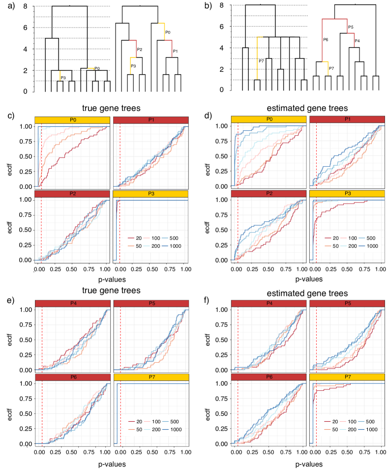
Figure 2: S12 datasets: true species trees and $p$-value distributions. For S12A (a) and S12B (b), we show the true multifurcating species trees in coalescent units (left) and an arbitrary resolution of the species tree used to test for polytomies (right). Branches P1, P2, and P4–P6 (red) represent arbitrary resolutions for which the null hypothesis is correct. Branches P0, P3, and P7 (yellow) are selected as examples for which the null hypothesis is incorrect. (c–f) The $p$-value distributions are shown as empirical cumulative distribution functions (ECDF) where the x-axis shows the $p$-value $x$ and the y-axis shows the percentage of the replicates (out of 50) with a $p$-value $\leq x$. Results are shown for four selected branches of S12A (c,d) and S12B (e,f) for both true gene trees (c,e) and estimated gene trees (d,f) with varying numbers of gene trees (line colors). Dashed vertical red line shows $p$-value$=0.05$. In red boxes, the intersection of the vertical line with each line shows the false positive rate. In yellow boxes, the intersection of the vertical line with each line shows one minus the false negative rate.

In this dataset, the true species trees are fully binary and therefore, the null hypothesis is never correct. Any failure to reject the null hypothesis is a false negative error. The inability to reject the null hypothesis should never be taken as accepting the null hypothesis because it can. simply indicate that the available data is insufficient to distinguish a polytomy from a short branch. An ideal test should be able to reject the null for long branches. However, for very short branches, failing to reject the null would be the expected behavior. It is worth contemplating the meaning of super short branches. For a haploid population size of $10^{5}$, a branch length of $10^{-4}$ CU corresponds to only ten generations. One can argue that such short branches, for most practical purposes, can be considered a polytomy. Thus, false negative errors among super short branches could perhaps be tolerated.

3 Results

3.1 Simulated datasets

We focus our discussions on $\alpha=0.05$, but we show full distributions of $p$-values in many places.

S12A and S12B

On the S12A tree, P1 and P2 are zero-length branches and therefore, the test should ideally fail to reject the null hypothesis for them. As desired, when true gene trees are used, $p$-values are uniformly distributed (Fig. 2c; note the linear empirical cumulative distribution functions for P1 and P2 with true gene trees). For example, the null hypothesis is rejected for 4% of replicates with 1000 gene trees. As expected, since the null is correct, the false positive rate does not increase as we increase the number of gene trees. Switching to estimated gene trees universally increases false positive errors (Fig 2d). For example for P1, we reject the null hypothesis in 12% of replicates using 1000 gene trees. The most severe case of false positive error rates occurs for branch P2, where 24% of replicates are rejected with 1000 gene trees. Thus, gene tree errors can, in fact, increase the false positive error rates, but the extent of the increase depends on the length of branches surrounding the tested branch.

On the S12A tree, we also examine two binary positive-length branches: P0, which is short (0.2 CU length) and the parent of a polytomy, and P3 (1 CU), which is longer and the child of a polytomy. On these, we desire that the null hypothesis should get rejected. The P3 branch is easily rejected in all replicates using true gene trees. With estimated gene trees, given 50 genes or more, the null is rejected in almost all cases, and is rejected in 66% of replicates with 20 genes. Thus, the power to reject this moderate length branch (corresponding to $2\times 10^{5}$ generations) is very high. For P0, which is rather short, the ability to reject the null hypothesis depends on the number of genes and similar to other branches, the power is higher for true gene trees. The false negative rates decrease as the number of genes increases; using 1000 gene trees, the null is rejected in all replicates with true gene trees and in 86% of replicates with estimated gene trees. Overall, the false negative rate is a function of the number of genes, the length of the branch, and gene tree error, as expected.

The S12B tree shows broadly similar results as S12A (Fig 2ef) but some differences are noteworthy. On the zero-length branches (P4, P5, and P6), as desired, the test fails to reject the null. However, false positives rates are a bit lower than expected by chance when true gene trees are used. For example, at $\alpha=0.05$, we barely ever reject the null hypothesis for either of these three branches. These lower than expected false positive rates may be due to the fact that each branch is considered independently in our test, but P4, P5, and P6 are very much dependent (they all resolve one high degree polytomy). Even using estimated gene trees, the false positive rate remains low. With estimated gene trees, for P4, we reject the null in 4% of replicates when we use 1000 gene trees and we never reject the null hypothesis otherwise (Fig 2f). For P5 and P6, the false positive rates is at most 8% and 4% with 1000 genes. While the false positive rates remain low with estimated gene trees, the rate seems to slightly increase with increased numbers of gene trees. Alongside the zero-length branches, we also study the branch P7 (length: 2 CU), which is adjacent to the polytomy. For this relatively long branch, we always reject the null hypothesis with true gene trees. With estimated gene trees, the false negative rate is only 16% with 20 gene trees and gradually drops to 0% at 200 genes or more.

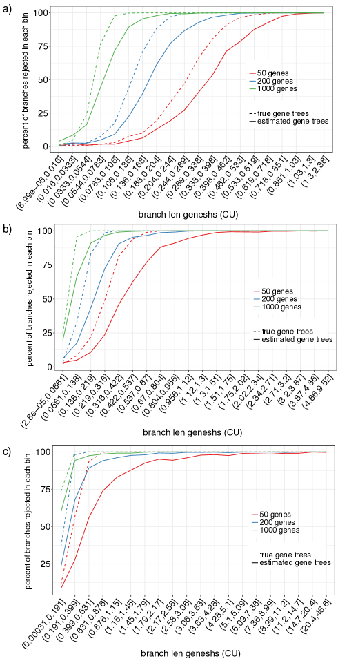
Figure 3: Polytomy test on S201 using estimated (solid) and true (dashed) gene trees for the different numbers of genes (colors) for model conditions with the tree height set to 500K (a), 2M (b), and 10M (c) generations. We show percentages of branches with the $p$-value $\leq 0.05$ (y-axis) for branch length ranges (x-axis), formed by dividing the log of the true CU branch lengths into 20 equisized bins.

S201

On the S201 datasets, we can only have false negative errors. We bin branches according to the log of their CU length into 20 categories and compute the percentage of branches that are rejected according to our test with $\alpha=0.05$ per bin (Fig 3). The false negative rate mostly depends on three factors: 1) the branch length, 2) the number of genes, and 3) whether true or estimated gene trees are used. The impact of all three factors is consistent with what one would expect for a reasonable statistical test. For the longest branches (e.g., $>1.5$ CU), the null hypothesis is rejected almost always even with as few as 50 genes and with our highly error-prone estimated gene trees. Using the true gene trees instead of estimated gene trees increases the power universally. For example, with 50 true gene trees, branches as short as $0.6$ CU are almost always rejected. Interestingly, the difference between estimated and true gene trees seems to reduce as the number of genes increase.

Reassuringly, as the number of genes increases, the power to reject the null hypothesis also increases. Thus, with 1000 genes, branches between 0.1–0.2 CU are rejected 99.9% of the times with true gene trees and 90.0% of the times with estimated gene trees. Branches below $\log(7/6)\approx 0.15$ are considered very short and can produce the anomaly zone Degnan and Rosenberg (2006); Degnan (2013). Branches in the 0.05–0.15 CU range are rejected 90.4% and 67.4% of times with 1000 true and estimated gene trees, respectively.

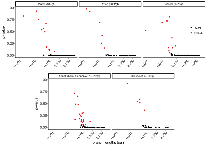
Figure 4: Polytomy test results for 5 different biological datasets using ASTRAL species trees, and all available gene trees. For each internal branch, we show its ASTRAL estimated CU length in log scale (x-axis) and its polytomy test $p$-value (y-axis). Points with $p<0.05$ are in black. For each dataset (panel), the number of genes is reported inside the parentheses in the title.

3.2 Biological dataset

On the biological datasets, the ability to reject the null hypothesis depends on the branch length and the effective number of gene trees (Figure 4). Most branches with the estimated length greater than $0.1$ CU had $p<0.05$. Datasets with more than a thousand genes (Aves and insects) had higher resolution and have $p<0.05$ for branches with the estimated length as lows as $0.035$ CU. Yet in all datasets except the Aves (where all gene trees include all species) there are some ranges of branch length (often above $0.1$ CU) where we are able to reject the null hypothesis for some branches but not for the others. This cannot be just due to random noise because estimated (not the unknown true) branch length is shown and two branches with the same length, have identical $n_{i}/n$ values. Instead, the reason is that the effective number of genes changes from one branch to another because some gene trees may not include enough species to define a quartet around some branches. The effective number of genes can also decline due to a lack of gene tree resolution, but this does not happen in our datasets, which include only binary gene trees (we will revisit this in the discussion section).

To further test the impact of the number of genes, for each dataset, we randomly subsampled gene trees ($1\%-100\%$ but no less than 20 gene trees) to find out how many genes are needed before we are able to reject the null hypothesis. We repeat this subsampling procedure 20 times, and show the average $p$-values across all 20 runs (Figures 5 and 6). In these analyses, we focus on selected branches of each empirical dataset. Note that in some downsampled datasets, occasionally branches have an effective number of genes that is smaller than $10$, violating our assumption A3; we exclude these branches.

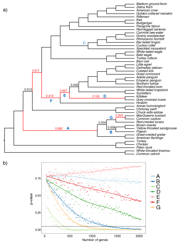
Figure 5: Polytomy test results on avian dataset. (a) ASTRAL species tree using binned ML gene trees. $p$-values greater than zero are reported on the branches, branches with $p>0.05$ are shown in red. (b) change in $p$-value with respect to the number of genes for the selected branches in the species tree (labeled in blue in panel a). We used ASTRAL species trees with the varying number of gene trees sampled uniformly (1%, 2%, 3%,…, 100% of gene trees but no less than 20), and repeated 20 times. We show average $p$-values (y-axis) versus the number of gene trees (y-axis). Solid horizontal line shows $p$-value$=0.05$.

For the avian datasets, 6 branches in the species tree could not be rejected as a polytomy at $\alpha=0.05$ even with all super gene trees (Figure 5a). These mostly belong to what has been called the wall-of-death Joseph and Buchanan (2015), a hypothesized rapid radiation at the base of Neoaves Jarvis et al. (2014); Swati Patel and Braun (2013). In subsampling super gene trees, we highlight seven selected branches (labeled A–G) as shown in Figure 5a. Interestingly, when we subsample super gene trees, several distinct patterns emerge for various branches. Most branches are easily rejected as a polytomy even with a small fraction of the data (e.g., C). For some shorter branches (e.g., G and B) rejecting a polytomy requires hundreds of super gene trees. Yet for others (e.g., D and perhaps F), we cannot reject the polytomy with the full dataset, but the pattern suggests that if we had more super gene trees, we may have been able to reject them as a polytomy. Finally, for some branches (e.g., A and G), increasing the number of genes does not lead to a substantial decrease in the $p$-value, suggesting that increasing the number of input trees may not be sufficient to resolve them.

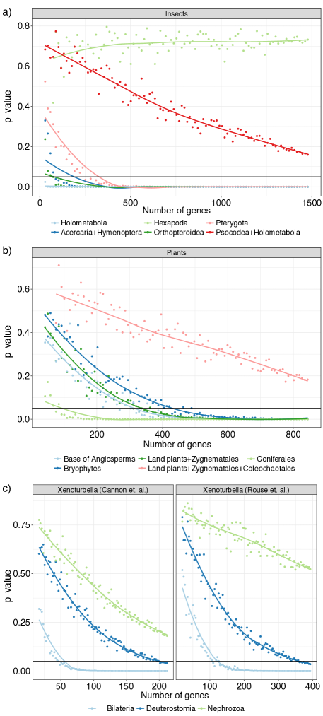
Figure 6: Polytomy test results for selected branches of (a) insects (b) plants, and (c) two Xenoturbella datasets. We used ASTRAL species trees with the varying number of gene trees sampled uniformly at random (1%, 2%,…, 100% of gene trees but no less than 20) repeated 20 times. We show average $p$-values (y-axis) versus the number of gene trees (x-axis). Solid horizontal line shows $p$-value$=0.05$. Cases with effective $n$ below 10 are excluded; for plants and Xenoturbella, we omit 1–4% because most replicates have $n<10$.

For the insect dataset we focus on 6 clades, Holometabola, Acercaria+Hymenoptera, Hexapoda, Orthopteroidea, Pterygota, and Psocodea+Holometabola; these all have been classified as having fairly strong support from the literature Sayyari et al. (2017), indicating that they enjoy robust support in the literature but some analyses reject them. As we reduce the number of genes, just like the avian dataset, we see three patterns (Figure 6a). For clades Holometabola, Acercaria+Hymenoptera, and Orthopteroidea, we get $p<0.05$ even with fewer than $100$ genes and for Pterygota with around 250 genes. We are not able to reject the null hypothesis for Psocodea+Holometabola with all gene trees, but the decreasing $p$-values suggest that this resolution could perhaps be resolved if we had several hundred more loci. The support for Hexapoda never decreases as we use more genes, suggesting that the relationship between insects and their close relatives (Collembola and Diplura, both considered insects in the past) may remain unresolved if we simply increase the number of genes. For this deep (around 450M years old) and undersampled node, $p$-values may fail to reduce either because of a true polytomy or because gene trees are estimated with high (perhaps biased) error.

In remaining datasets (plants and Xenoturbella), all important branches that we studied saw decreasing $p$-values as the number of gene trees increase (Figure 6b). In the plant dataset, having around 400 genes seems sufficient for most branches of interest, including the monophyly of Bryophytes and the resolution of Amborella as sister to all the remaining flowering plants. The branch that puts Zygnematales as sister to land plants is rejected as a polytomy with about 350 genes. However, the correct relationship between Chara and Coleochaetales remains hard to resolve. Even with the full dataset, a polytomy is not rejected, though the decreasing $p$-values point to the possibility that this relationship would have been resolved had we had more genes.

The Xenoturbella datasets both have three focal branches, surrounding the position of Xenacoelomorpha. The branch labeled Bilateria, which has Xenacoelomorpha and Nephrozoa as daughters branches in both papers, can be resolved at $\alpha=0.05$ with as few as 50 (Cannon) or 100 (Rouse) gene trees (Figure 6c). However, pinpointing the position of Xenacoelomorpha also depends on the branch labeled Nephrozoa, which puts Xenacoelomorpha as sister to a clade containing Protostomia and Deuterostomia. The null hypothesis that this branch may be a polytomy is not rejected in either dataset, but a pattern of decreasing $p$-values with more loci can be discerned. Thus, both datasets are best understood as leaving the relationships between Protostomia, Xenacoelomorpha, and the rest of Deuterostomia as uncertain with some evidence that Xenacoelomorpha is at the base of Nephrozoa. Remarkably, patterns of difficulty in resolving branches are similar across the two independent datasets with different taxon and gene selection.

4 Discussion

We introduced a new test for rejecting the null hypothesis that a branch in the species tree should be replaced by a polytomy. Unlike existing tests, our new test considers gene tree discordance due to ILS, as modeled by the MSC model. In several simulations, we showed that the test behaves as expected. The null hypothesis is often retained for true polytomies and is often rejected for binary nodes, unless when the true branch lengths are very short. The power to reject the null hypothesis for binary relationships increases with longer branches or with more gene trees and is reduced with gene tree estimation error. Gene tree error can also, in some cases, increase the false positive rate.

4.1 Power

Overall, even when we have 1000 genes, it is rare that we can reject the null for branches shorter than 0.03 CU. A branch of length 0.03 corresponds to 6000 generations in our simulations. One can argue that failing to resolve a branch that corresponds to such short evolutionary times (roughly 60K years with a generation time of 10 years) can perhaps be tolerated. Mathematically, given a sufficiently large unbiased sample of gene trees, even infinitesimally short branches can be distinguished from a polytomy. In practice, however, extremely short branches should be treated with suspicion as our input gene trees invariably are not perfect samples from the MSC distribution.

In our biological analyses, we saw that subsampling genes and tracking trajectories of the $p$-value may be helpful in predicting the number of required genes to resolve a branch. The approach we presented can be used in other biological data as well. However, we caution that such predictions should be interpreted with the limitations of our proposed test in mind. Many factors such as gene tree error and other sources of discordance can contribute to deviations from MSC, and such deviations may render the predictions inaccurate. But if such predictions are to be made, a natural question arises: How does the number of genes impact the power?

(a) (b)  

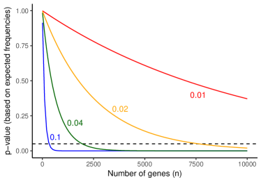
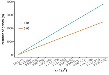
Figure 7: Impact of the number of genes on $p$-value (a) The $p$-value computed for the different number of gene trees (x-axis) for four different short branch lengths (colors) when the observed frequencies exactly match the expected frequencies given that branch length. Dashed horizontal line shows $p$-value$=0.05$; it intersects at 331 for 0.1 CU, 1949 for 0.04 CU, 7641 for 0.02 CU, and 30259 for 0.01 CU (not shown). (b) The required number of genes (y-axis) to reject the null hypothesis with a $p$-value of 0.05 or 0.01 for various branch lengths (x-axis) assuming that the observed frequencies match the expected frequencies. Note that the x-axis scales with $\frac{1}{x^{2}}$.

We can easily compute the required number of genes for rejecting the null hypothesis assuming the expected frequencies match observed frequencies (Fig. 7a). For example, while for a branch of length 0.1 CU we only need $\approx$300 genes before we can reject it as a polytomy, for a branch of length 0.02 (i.e., 5 times shorter), we need $\approx$7500 genes (i.e., 25 times more). For a quartet species tree, $n_{1}>\max(n_{2},n_{3})$ with arbitrarily high probability if the number of genes grows as $\frac{\log N}{x^{2}}$ Shekhar et al. (2017). More broadly, the number of genes required for correct species tree estimation using ASTRAL is proven to grow proportionally to $\log N$ and to $x^{-2}$ Shekhar et al. (2017). Similarly, for any given branch length, we can numerically compute the minimum number of required genes to obtain a given $p$-value (e.g., $0.05$). Assuming the observed frequencies match the expectations, we observe that the required number of genes grows linearly with $\frac{1}{x^{2}}$ (Fig. 7b). In fact, Figure 7b gives us a way to estimate the level of “resolution” that a dataset can provide. For example, 300 genes can reject the null for branches of $\approx$0.1 CU but if we quadruple the number of genes to 1200, our resolution is increased two-folds to branches of $\approx$0.05 CU. Note that gene tree error would increase these requirements and hence these should be treated as ballpark estimates. These estimates also assume we have $N=4$ species.

The test we presented has no guarantees of maximal power. Other tests, such as likelihood ratio, may be more powerful. Moreover, it can be argued that our test is conservative in how it handles $N>4$. When multiple quartets are available around a branch, we use their fraction supporting the $\mathcal{B}$ topology as the contribution of that gene to $n_{1}$. Thus, whether we have one quartet or a hundred quartets, we count each gene tree as one observation of our multinomial distribution. This is the most conservative approach to deal with the unknown dependencies between quartets. The most liberal approach would consider quartets to be fully independent, increasing the degrees of the freedom of the chi-square distribution to $2m$ instead of $2$. Such a test would be more powerful but would be based on invalid independence assumptions that may raise false positive rates. An ideal test would need to model the intricate dependence structure of quartets, a task that is very difficult Erdos et al. (1999).

Finally, note that our test of polytomy relates to branch lengths in coalescent units. A branch of length zero in coalescent units will have length zero in the unit of time (or generations) if we keep the population size fixed. Mathematically, we can let the population size grow infinitely. For a mathematical model where the population size grows asymptotically faster than the time, one can have branches that converge to zero in length even though the branch length in time goes to infinity. This is just a mathematical construct with no biological meaning. Nevertheless, it helps to remind us that a very short branch in the coalescent unit (which our test may fail to reject as a polytomy) may be short not because the time was short but because the population size was large. Branches between 0.1 and 0.2 CU were not rejected as a polytomy by our test $\approx$10% of times even with 1000 genes. A length of 0.1 CU can correspond to 10M generations if the haploid population size is 100M.

4.2 Divergence from the MSC model and connections to localPP

The $p$-value from our proposed polytomy test has a close connection to the localPP branch support. Both measures assume the MSC model and both are a function of quartet scores (i.e., $n_{i}/n$). As the quartet score of the species tree topology and the number of genes increases, both localPP and $1-p$-value increase (Fig. 8a). When localPP of a branch is close to 1.0, the polytomy null hypothesis is always rejected. However, the two measures are not identical. Interestingly, there are some conditions where localPP is higher than 0.95 but the polytomy null hypothesis is not rejected at the 0.05 level (Fig. 8a). When the frequencies follow expectations of the MSC model, $1-p$-value of the polytomy test is smaller than the localPP.

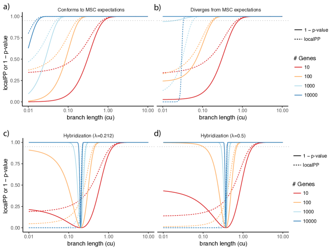
Figure 8: The polytomy test versus localPP. For various branch lengths (x-axis; log scale) and various numbers of gene trees (colors), we show (y-axis) both the localPP (dashed line) and $1-p$-value of the polytomy test (solid line). (a) The quartet frequencies follow MSC expectations: $\frac{n_{1}}{n}=1-\frac{2}{3}e^{-x},\frac{n_{2}}{n}=\frac{n_{3}}{n}=\frac{1}{2}\frac{2}{3}e^{-x}$. (b) The quartet frequencies diverge from the MSC expectations so that $n_{2}$ is 20% larger than $n_{3}$. $\frac{n_{1}}{n}=1-\frac{2}{3}e^{-x},\frac{n_{2}}{n}=\frac{6}{11}\frac{2}{3}e^{-x},\frac{n_{3}}{n}=\frac{5}{11}\frac{2}{3}e^{-x}$. (c,d) quartet frequencies follow the MSC+gene flow model, as analyzed by Solís-Lemus et al. Solís-Lemus et al. (2016). For a species tree with a hybridization at the base (see Fig. 2 of Solís-Lemus et al. (2016)) with inheritance probabilities $\lambda=0.1$ (c) and $\lambda=0.5$ (d), following Solís-Lemus et al., we set $\frac{n_{1}}{n}=(1-\lambda)^{2}(1-\frac{2}{3}e^{-x})+2\lambda(1-\lambda)(1-e^{-x/2}+\frac{1}{3}e^{-x-4})+\lambda^{2}(1-\frac{2}{3}e^{-x/2})$ and $n_{2}=n_{3}=\frac{n-n_{1}}{2}$. The dotted horizontal gray line shows $p$-value$=0.05$.

It is important to remember that our test relies on the properties of the MSC model. If observed quartet frequencies diverge from the expectations of the MSC model systematically (as opposed to by natural variation), the behavior of our proposed test can change. For example, if $n_{2}$ is substantially larger than $n_{3}$, rejecting the null hypothesis becomes easier (Fig. 8b). This should not come as a surprise because this type of deviation from the MSC model makes the quartet frequencies even more diverged from $\frac{1}{3}$ than what is expected under the MSC model. On real data, several factors can may contribute to deviations from MSC. For example, incorrect homology detection in real datasets is possible (e.g., see Springer and Gatesy (2017) for possible homology issues with the avian dataset) and can lead to deviations.

Another source of deviation is gene flow, which can impact the gene tree distributions. Solís-Lemus et al. have identified anomaly zone conditions where the species tree topology has lower quartet frequencies compared to the alternative topologies Solís-Lemus et al. (2016). Since the localPP measure does not model gene flow, under those conditions, it will be misled, giving low posterior probability to the species tree topology in the presence of gene flow (Fig. 8c). For example, if $\lambda=0.1$ (meaning that 10% of genes are impacted by the horizontal gene flow), for branches of length 0.1 or shorter, localPP will be zero. The presence of the gene flow also impacts the test of the polytomy. For the species tree defined by Solís-Lemus et al. (Fig. 1 of  Solís-Lemus et al. (2016)), when internal branches are short enough, there exist conditions where the gene flow and ILS combined result in quartet frequencies being equal to $\frac{1}{3}$ for all the three alternatives. It is clear that our test will not be able to distinguish such a scenario from a real polytomy (Fig. 8cd). One is tempted to argue that perhaps high levels of gene flow between sister branches should favor the outcome that the null is not rejected. However, this argument fails to explain the observation that for any value of $\lambda$, the null hypothesis is retained only with very specific settings of surrounding internal branch lengths (Fig. 8cd ). Thus, we simply caution the reader about the interpretation when gene flow and other sources of bias are suspected.

4.3 The effective number of gene trees

It is important to note that the effective number of gene trees (effective-$n$) can change across branches of the same species tree. Missing data can reduce the number of genes that have at least one taxon from a quartet defined around the branch of interest. In our biological datasets, various branches of the same dataset often have a wide range of effective $n$ (Fig 9a), especially for the two transcriptomic datasets (insects and plants) with lots of missing data. The only exception is the avian dataset, where our super gene trees always include all the taxa.

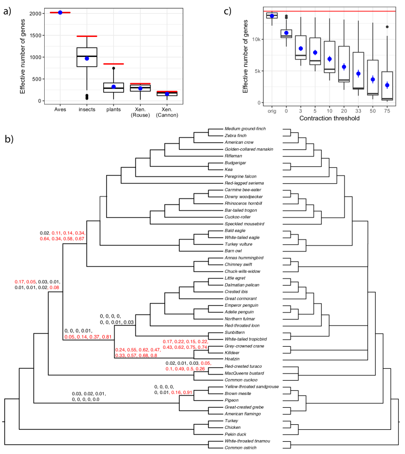
Figure 9: Effective $n$ and results on the unbinned avian dataset. (a) Distributions of effective $n$ (y-axis) across different branches of each empirical dataset (x-axis). We show boxplots (black) as well as mean and standard error (blue). The total number of genes ($n$) is shown as a red horizontal line. (b) ASTRAL-III species tree estimated based on 14,446 unbinned gene trees with branches up to 10% support contracted. For each branch, we show eight $p$-values that are computed, respectively, with respect to gene trees where branches with support up to 0%, 3%, 5%, 10% (top), 20%, 33%, 50%, or 75% (bottom) are contracted. Branches with no values have only 0 $p$-values (to three decimal points). $p$-values above 0.05 are in red. We also show the multifurcating species tree where all five branches that have $p$-values$<0.05$ according to the 10% threshold are contracted (the left facing tree). (c) Similar to (a), we show distributions of effective $n$ (y-axis) across branches of the avian species tree with all 14,446 original unbinned trees (orig) or with gene tree branches with low support contracted (x-axis).

A second factor that can reduce the effective $n$ is multifurcations in input gene trees. If all the quartets around a branch are unresolved in an input gene tree, that gene tree does not count towards the effective $n$. Our biological datasets had binary gene trees. However, as recently shown Zhang et al. (2017), removing branches with very low support can help addressing gene tree error. To demonstrate this, we revisit the avian dataset. The purpose of using super gene trees instead of normal (unbinned) gene trees was to reduce the gene tree estimation error. Alternatively, one can simply remove branches with support at or below a certain threshold in gene trees and use the resulting tree as input to ASTRAL Zhang et al. (2017). With this procedure and the support threshold set to 10%, we generated a new ASTRAL tree based on all 14,446 unbinned gene trees from the avian dataset Jarvis et al. (2014); Mirarab et al. (2014) (Fig 9b). The resulting tree was largely congruent with the ASTRAL tree on super gene trees and with reference phylogenies form the original publication Jarvis et al. (2014).

We tested how the effective $n$ and $p$-values change as a result of contracting low support branches. Simply contracting branches with 0% support reduces the median effective $n$ from 13,791 to 10,523. Further contracting branches with support up to 3% – 75% gradually reduces the effective $n$ all the way to a median of 610 (Fig 9c). The $p$-values tend to decrease as we increase the threshold for contraction (Fig 9b). Several branches fail to reject the null hypothesis regardless of the threshold chosen. Others reject the null hypothesis with lower levels of contraction but not with the higher levels, showing that the reduced effective $n$ can reduce the power. For one branch, interestingly, the null is not rejected if we contract up to 0% and 3% support or if we contract up to 75%, but is rejected otherwise. This pattern may have a subtle explanation. With gene trees that include low support branches (up to 3%), we are unable to reject the null hypothesis perhaps because gene tree error creates a uniform distribution of quartets around this branch. As we further remove low support branches from the gene trees, we start to see quartet frequencies that favor the ASTRAL resolution perhaps because noise is removed and the actual signal can be discerned. Finally, with aggressive filtering of gene tree branches, effective $n$ becomes so low that the test simply does not have the power to reject the null. These interesting patterns suggest that dealing with gene tree error by contracting low support branches may be possible, but the choice of the best threshold is not obvious. Future studies should further consider this question.

4.4 Interpretation

In the light of the dependence of our test on the MSC properties, we offer an alternative description of the test. A safe way to interpret the results of the test, regardless of the causes of gene tree discordance, is to formulate the null hypothesis as follows.

Null hypothesis:

The estimated gene tree quartets around the branch $\mathcal{B}$ support all three NNI rearrangements around the branch in equal numbers.

This is the actual null hypothesis that we test. Under our assumptions, this hypothesis is equivalent to branch $\mathcal{B}$ being a polytomy. Under more complex models, such as gene flow + ILS, this null hypothesis holds true for polytomies but also for some binary networks.

The judicious application of our test will preselect the branches where a polytomy null hypothesis is tested and examines the $p$-value only for those branches. When many branches are tested, one arguably needs to correct for multiple hypothesis testing, further reducing the power of the test. Corrections such as Bonferroni or FDR Benjamini and Hochberg (1995) can be employed (but we did not apply them in our large scale tests that did not target specific hypotheses). However, note that even though we formulate the polytomy as a null hypothesis, in reality, we expect that in most cases the branch has positive branch length. Thus, we expect to reject the null often, in contrast to usual applications of the frequentist test. The analyst should specify in advance the branches for which a polytomy null hypothesis is reasonable. This adds subjectivity, but such problems are always encountered with frequentist tests, and ours is no exception. Our test also suffers from all the various criticisms leveled against the frequentist hypothesis testing Anderson et al. (2000) and the interpretation has to avoid all the common pitfalls Goodman (2008).

5 Conclusions

We presented a statistical test, implemented in ASTRAL, for the null hypothesis that a branch of a species tree is a polytomy given a set of gene trees. Our test, which relies on the properties of the multi-species coalescent model, performed well on simulated and real data. As expected, its power was a function of branch length, the number of genes, and the gene tree estimation error.

supplementary

All data, R script, and results are available at https://github.com/esayyari/polytomytest.

Abbreviations

The following abbreviations are used in this manuscript:

ILS: Incomplete Lineage Sorting
MSC: Multi-Species Coalescent
CU: Coalescent Unit

References

- Bapteste et al. (2013) Bapteste, E.; van Iersel, L.; Janke, A.; Kelchner, S.; Kelk, S.; McInerney, J.O.; Morrison, D.A.; Nakhleh, L.; Steel, M.; Stougie, L.; Whitfield, J. Networks: expanding evolutionary thinking. Trends in Genetics 2013, 29, 439 – 441.
- Nakhleh (2011) Nakhleh, L., Evolutionary Phylogenetic Networks: Models and Issues. In Problem Solving Handbook in Computational Biology and Bioinformatics; Heath, L.S.; Ramakrishnan, N., Eds.; Springer US: Boston, MA, 2011; pp. 125–158.
- Hoelzer and Meinick (1994) Hoelzer, G.A.; Meinick, D.J. Patterns of speciation and limits to phylogenetic resolution. Trends in Ecology & Evolution 1994, 9, 104–107.
- Suh (2016) Suh, A. The phylogenomic forest of bird trees contains a hard polytomy at the root of Neoaves. Zoologica Scripta 2016, 45, 50–62.
- Arntzen et al. (2007) Arntzen, J.W.; Themudo, G.E.; Wielstra, B. The phylogeny of crested newts (Triturus cristatus superspecies) nuclear and mitochondrial genetic characters suggest a hard polytomy, in line with the paleogeography of the centre of origin. Contributions to Zoology 2007, 76.
- Townsend et al. (2012) Townsend, J.P.; Su, Z.; Tekle, Y.I. Phylogenetic Signal and Noise: Predicting the Power of a Data Set to Resolve Phylogeny. Systematic Biology 2012, 61, 835.
- Maddison (1989) Maddison, W. Reconstructing character evolution on polytomous cladograms. Cladistics 1989, 5, 365–377.
- Chojnowski et al. (2008) Chojnowski, J.L.; Kimball, R.T.; Braun, E.L. Introns outperform exons in analyses of basal avian phylogeny using clathrin heavy chain genes. Gene 2008, 410, 89–96.
- Jackman et al. (1999) Jackman, T.R.; Larson, A.; de Queiroz, K.; Losos, J.B.; Cannatella, D. Phylogenetic Relationships and Tempo of Early Diversification in Anolis Lizards. Systematic Biology 1999, 48, 254–285.
- Walsh et al. (1999) Walsh, H.E.; Kidd, M.G.; Moum, T.; Friesen, V.L. Polytomies and the power of phylogenetic inference. Evolution 1999, 53, 932–937.
- Swofford et al. (1996) Swofford, D.L.; Olsen, G.J.; Waddell, P.J.; Hillis, D.M. Phylogenetic inference. In Molecular systematics (2nd ed.); Hillis, D.M.; Moritz, C.; Mable, B.K., Eds.; Sinauer Associates, Inc.: Sunderland, Massachusetts, 1996; pp. 407–514.
- Swofford (2003) Swofford, D.L., PAUP*. Phylogenetic Analysis Using Parsimony (*and other methods). Version 4.; Sinauer Associates: Sunderland, Massachussets, 2003.
- Braun and Kimball (2001) Braun, E.L.; Kimball, R.T. Polytomies, the power of phylogenetic inference, and the stochastic nature of molecular evolution: a comment on Walsh et al. (1999). Evolution 2001, 55, 1261–1263.
- Anisimova et al. (2006) Anisimova, M.; Gascuel, O.; Sullivan, J. Approximate Likelihood-Ratio Test for Branches: A Fast, Accurate, and Powerful Alternative. Systematic Biology 2006, 55, 539–552.
- Lewis et al. (2005) Lewis, P.O.; Holder, M.T.; Holsinger, K.E. Polytomies and Bayesian phylogenetic inference. Systematic Biology 2005, 54, 241–253.
- Slowinski (2001) Slowinski, J.B. Molecular Polytomies. Molecular Phylogenetics and Evolution 2001, 19, 114–120.
- Degnan and Rosenberg (2009) Degnan, J.H.; Rosenberg, N.A. Gene tree discordance, phylogenetic inference and the multispecies coalescent. Trends in Ecology and Evolution 2009, 24, 332–340.
- Maddison (1997) Maddison, W.P. Gene Trees in Species Trees. Systematic Biology 1997, 46, 523–536.
- Poe and Chubb (2004) Poe, S.; Chubb, A.L. Birds in a bush: five genes indicate explosive evolution of avian orders. Evolution; international journal of organic evolution 2004, 58, 404–415.
- Rannala and Yang (2003) Rannala, B.; Yang, Z. Bayes Estimation of Species Divergence Times and Ancestral Population Sizes Using DNA Sequences From Multiple Loci. Genetics 2003, 164, 1645–1656.
- Pamilo and Nei (1988) Pamilo, P.; Nei, M. Relationships between gene trees and species trees. Molecular biology and evolution 1988, 5, 568–583.
- Heled and Drummond (2010) Heled, J.; Drummond, A.J. Bayesian inference of species trees from multilocus data. Molecular Biology and Evolution 2010, 27, 570–580.
- Liu (2008) Liu, L. BEST: Bayesian estimation of species trees under the coalescent model. Bioinformatics 2008, 24, 2542–2543.
- Chifman and Kubatko (2014) Chifman, J.; Kubatko, L.S. Quartet Inference from SNP Data Under the Coalescent Model. Bioinformatics 2014, 30, 3317–3324.
- Bryant et al. (2012) Bryant, D.; Bouckaert, R.; Felsenstein, J.; Rosenberg, N.A.; Roychoudhury, A. Inferring species trees directly from biallelic genetic markers: Bypassing gene trees in a full coalescent analysis. Molecular Biology and Evolution 2012, 29, 1917–1932.
- Mirarab et al. (2014) Mirarab, S.; Reaz, R.; Bayzid, M.S.; Zimmermann, T.; Swenson, M.S.; Warnow, T. ASTRAL: genome-scale coalescent-based species tree estimation. Bioinformatics 2014, 30, i541–i548.
- Mirarab and Warnow (2015) Mirarab, S.; Warnow, T. ASTRAL-II: coalescent-based species tree estimation with many hundreds of taxa and thousands of genes. Bioinformatics 2015, 31, i44–i52.
- Zhang et al. (2017) Zhang, C.; Sayyari, E.; Mirarab, S. ASTRAL-III: Increased Scalability and Impacts of Contracting Low Support Branches. Comparative Genomics; Meidanis, J.; Nakhleh, L., Eds.; Springer International Publishing: Cham, 2017; pp. 53–75.
- Larget et al. (2010) Larget, B.R.; Kotha, S.K.; Dewey, C.N.; Ané, C. BUCKy: Gene tree/species tree reconciliation with Bayesian concordance analysis. Bioinformatics 2010, 26, 2910–2911.
- Sayyari and Mirarab (2016) Sayyari, E.; Mirarab, S. Fast Coalescent-Based Computation of Local Branch Support from Quartet Frequencies. Molecular Biology and Evolution 2016, 33, 1654–1668.
- Allman et al. (2011) Allman, E.S.; Degnan, J.H.; Rhodes, J.A. Identifying the rooted species tree from the distribution of unrooted gene trees under the coalescent. J. Math. Biol. 2011, 62, 833–862.
- Zar (2007) Zar, J.H. Biostatistical Analysis (5th Edition); Prentice-Hall, Inc.: Upper Saddle River, NJ, USA, 2007.
- Koehler and Larntz (1980) Koehler, K.J.; Larntz, K. An Empirical Investigation of Goodness-of-Fit Statistics for Sparse Multinomials. Journal of the American Statistical Association 1980, 75, 336–344.
- Read and Cressie (1988) Read, T.R.C.; Cressie, N.A.C. Goodness-of-fit statistics for discrete multivariate data; Springer-Verlag New York, 1988.
- Hoschek (2004) Hoschek, W. The Colt distribution: Open source libraries for high performance scientific and technical computing in JAVA; CERN, Geneva, Switzerland, 2004.
- Sayyari et al. (2017) Sayyari, E.; Whitfield, J.B.; Mirarab, S. Fragmentary Gene Sequences Negatively Impact Gene Tree and Species Tree Reconstruction. Molecular Biology and Evolution 2017, 34, 3279–3291.
- Jarvis et al. (2014) Jarvis, E.D.; Mirarab, S.; Aberer, A.J.; Li, B.; Houde, P.; Li, C.; Ho, S.Y.W.; Faircloth, B.C.; Nabholz, B.; Howard, J.T.; Suh, A.; Weber, C.C.; da Fonseca, R.R.; Li, J.; Zhang, F.; Li, H.; Zhou, L.; Narula, N.; Liu, L.; Ganapathy, G.; Boussau, B.; Bayzid, M.S.; Zavidovych, V.; Subramanian, S.; Gabaldón, T.; Capella-Gutiérrez, S.; Huerta-Cepas, J.; Rekepalli, B.; Munch, K.; Schierup, M.H.; Lindow, B.; Warren, W.C.; Ray, D.; Green, R.E.; Bruford, M.W.; Zhan, X.; Dixon, A.; Li, S.; Li, N.; Huang, Y.; Derryberry, E.P.; Bertelsen, M.F.; Sheldon, F.H.; Brumfield, R.T.; Mello, C.V.; Lovell, P.V.; Wirthlin, M.; Schneider, M.P.C.; Prosdocimi, F.; Samaniego, J.A.; Velazquez, A.M.V.; Alfaro-Núñez, A.; Campos, P.F.; Petersen, B.; Sicheritz-Ponten, T.; Pas, A.; Bailey, T.; Scofield, P.; Bunce, M.; Lambert, D.M.; Zhou, Q.; Perelman, P.; Driskell, A.C.; Shapiro, B.; Xiong, Z.; Zeng, Y.; Liu, S.; Li, Z.; Liu, B.; Wu, K.; Xiao, J.; Yinqi, X.; Zheng, Q.; Zhang, Y.; Yang, H.; Wang, J.; Smeds, L.; Rheindt, F.E.; Braun, M.J.; Fjeldså, J.; Orlando, L.; Barker, F.K.; Jønsson, K.A.; Johnson, W.; Koepfli, K.P.; O?Brien, S.; Haussler, D.; Ryder, O.A.; Rahbek, C.; Willerslev, E.; Graves, G.R.; Glenn, T.C.; McCormack, J.E.; Burt, D.W.; Ellegren, H.; Alström, P.; Edwards, S.V.; Stamatakis, A.; Mindell, D.P.; Cracraft, J.; Braun, E.L.; Warnow, T.; Jun, W.; Gilbert, M.T.P.; Zhang, G. Whole-genome analyses resolve early branches in the tree of life of modern birds. Science 2014, 346, 1320–1331.
- Mirarab et al. (2014) Mirarab, S.; Bayzid, M.S.; Boussau, B.; Warnow, T. Statistical binning enables an accurate coalescent-based estimation of the avian tree. Science 2014, 346, 1250463–1250463.
- Rouse et al. (2016) Rouse, G.W.; Wilson, N.G.; Carvajal, J.I.; Vrijenhoek, R.C. New deep-sea species of Xenoturbella and the position of Xenacoelomorpha. Nature 2016, 530, 94–97.
- Cannon et al. (2016) Cannon, J.T.; Vellutini, B.C.; Smith, J.; Ronquist, F.; Jondelius, U.; Hejnol, A. Xenacoelomorpha is the sister group to Nephrozoa. Nature 2016, 530, 89–93.
- Wickett et al. (2014) Wickett, N.J.; Mirarab, S.; Nguyen, N.; Warnow, T.; Carpenter, E.J.; Matasci, N.; Ayyampalayam, S.; Barker, M.S.; Burleigh, J.G.; Gitzendanner, M.A.; Ruhfel, B.R.; Wafula, E.; Der, J.P.; Graham, S.W.; Mathews, S.; Melkonian, M.; Soltis, D.E.; Soltis, P.S.; Miles, N.W.; Rothfels, C.J.; Pokorny, L.; Shaw, A.J.; DeGironimo, L.; Stevenson, D.W.; Surek, B.; Villarreal, J.C.; Roure, B.; Philippe, H.; DePamphilis, C.W.; Chen, T.; Deyholos, M.K.; Baucom, R.S.; Kutchan, T.M.; Augustin, M.M.; Wang, J.; Zhang, Y.; Tian, Z.; Yan, Z.; Wu, X.; Sun, X.; Wong, G.K.S.; Leebens-Mack, J. Phylotranscriptomic analysis of the origin and early diversification of land plants. Proceedings of the National Academy of Sciences 2014, 111, 4859–4868.
- Mallo et al. (2016) Mallo, D.; De Oliveira Martins, L.; Posada, D. SimPhy : Phylogenomic Simulation of Gene, Locus, and Species Trees. Systematic Biology 2016, 65, 334–344.
- Fletcher and Yang (2009) Fletcher, W.; Yang, Z. INDELible: A flexible simulator of biological sequence evolution. Molecular Biology and Evolution 2009, 26, 1879–1888.
- Price et al. (2010) Price, M.N.; Dehal, P.S.; Arkin, A.P. FastTree 2 – Approximately Maximum-Likelihood Trees for Large Alignments. PLoS ONE 2010, 5, e9490.
- Degnan and Rosenberg (2006) Degnan, J.H.; Rosenberg, N.A. Discordance of Species Trees with Their Most Likely Gene Trees. PLoS Genetics 2006, 2, e68.
- Degnan (2013) Degnan, J.H. Anomalous Unrooted Gene Trees. Systematic Biology 2013, 62, 574–590.
- Joseph and Buchanan (2015) Joseph, L.; Buchanan, K.L. A quantum leap in avian biology. Emu 2015, 115, 1–5.
- Swati Patel and Braun (2013) Swati Patel, R.T.K.; Braun, E.L. Error in Phylogenetic Estimation for Bushes in the Tree of Life. Journal of Phylogenetics & Evolutionary Biology 2013, 1, 1–10.
- Shekhar et al. (2017) Shekhar, S.; Roch, S.; Mirarab, S. Species tree estimation using ASTRAL: how many genes are enough? IEEE/ACM Transactions on Computational Biology and Bioinformatics 2017, PP, 1–1.
- Erdos et al. (1999) Erdos, P.; Steel, M.; Szekely, L.; Warnow, T. A few logs suffice to build (almost) all trees: Part II. Theoretical Computer Science 1999, 221, 77–118.
- Solís-Lemus et al. (2016) Solís-Lemus, C.; Yang, M.; Ané, C. Inconsistency of Species Tree Methods under Gene Flow. Systematic Biology 2016, 65, 843–851.
- Springer and Gatesy (2017) Springer, M.S.; Gatesy, J. On the importance of homology in the age of phylogenomics. Systematics and Biodiversity 2017, pp. 1–19.
- Benjamini and Hochberg (1995) Benjamini, Y.; Hochberg, Y. Controlling the false discovery rate: a practical and powerful approach to multiple testing. Journal of the Royal Statistical Society. 1995, 57, 289–300.
- Anderson et al. (2000) Anderson, D.R.; Burnham, K.P.; Thompson, W.L. Null Hypothesis Testing: Problems, Prevalence, and an Alternative. The Journal of Wildlife Management 2000, 64, 912–923.
- Goodman (2008) Goodman, S. A Dirty Dozen: Twelve P-Value Misconceptions. Seminars in Hematology 2008, 45, 135 – 140.