DESY 17-120 KEK Preprint 2017–22 SLAC–PUB–17129 August, 2017
Improved Formalism for Precision Higgs Coupling Fits
Tim Barklowa, Keisuke Fujiib, Sunghoon Jungac, Robert Karld, Jenny Listd, Tomohisa Ogawab, Michael E. Peskina, and Junping Tiane
a SLAC,
Stanford University, Menlo Park, CA 94025, USA
b High Energy Accelerator Research Organization (KEK), Tsukuba,
Ibaraki, JAPAN
c Dept. of Physics and Astronomy, Seoul National
Univ.,
Seoul 08826, KOREA
d DESY,
Notkestrasse 85, 22607 Hamburg, GERMANY
e ICEPP, University of Tokyo, Hongo, Bunkyo-ku, Tokyo,
113-0033, JAPAN
ABSTRACT
Future colliders give the promise of model-independent determinations of the couplings of the Higgs boson. In this paper, we present an improved formalism for extracting Higgs boson couplings from data, based on the Effective Field Theory description of corrections to the Standard Model. We apply this formalism to give projections of Higgs coupling accuracies for stages of the International Linear Collider and for other proposed colliders.
Submitted to Physical Review D
1 Introduction
One of the most important opportunities provided by future colliders is that of determining the couplings of the Higgs boson with high precision and in a model-independent way. By now, many studies have made projections of the accuray with which Higgs couplings can be determined at proposed colliders [1, 2, 3, 4, 5, 6, 7]. Most of these studies are based on the formalism, in which each Standard Model Higgs coupling is multiplied by an independent factor and these factors are fit to expected measurements. The assumption is that introducing a large number of parameters leads to coupling determinations with a great deal of model-independence.
An alternative method, described in [8, 9], takes a different point of view. This method begins from the assumption that the corrections to the Standard Model (SM) due to new physics can be parametrized by the addition of higher-dimension operators to the renormalizable (dimension 4) SM Lagrangian. We have come to realize that this approach is more correct in the way it takes into account the variety of effects that might arise from new physics. In addition, it allows us to incorporate powerful constraints from gauge invariance, and to make use of new observables that have not previously been considered in Higgs coupling fits. In this paper, we will formalize this approach, describe its advantages, and present projections of Higgs coupling accuracy for future colliders based on this formalism. Some recent analyses with similar ingredients but different emphases can be found in [10, 11, 12, 13, 14, 15, 16].
In particular, we make the assumption that the deviations from the SM predictions for the Higgs couplings can be represented by the addition of dimension-6 operators. There are a large number of possible dimension-6 operator coefficients—84 in all—but only a manageable number of these play a role in the analysis of Higgs couplings. We will refer to the effective field theory (EFT) operator coefficients as , to distinguish them from the .
The EFT approach is largely now adopted in the analysis of Higgs coupling data from the LHC; see [17]. However, the information on the EFT coefficients that will come from future colliders will be much more complete and specific. In fact, it is shown in some detail in the accompanying paper [18] that data from future colliders can determine, independently and without ambiguity, all of the dimension-6 EFT coefficients that contribute directly to Higgs boson production and decay processes at those colliders. We can then use the EFT approach to provide estimates of Higgs boson couplings that are completely model-independent as long as the general framework of the EFT is valid.
Because one EFT operator can be exchanged for another by the use of the equations of motion, there are several different conventions used for the . In this paper, we will use a variant of the “Warsaw basis” introduced in [19]. The notation, and detailed formulae for the linear deviations of the Higgs couplings, can be found in [18]. A similar set of formulae in the “SILH basis” [8, 9] can be found in [14, 20].
2 Why is model-dependent?
Let’s get right to the point: Why is a formalism based on not model-independent?
For Higgs decays to fermions, the corrections to the Standard Model are described phenomenologically by a single operator whose effect can be described by a rescaling. The same is true for decays to or . However, for the Higgs coupling to and , this is not correct. The EFT actually leads to two distinct structures. We can represent the Higgs- interaction as parametrized by two coefficients , ,
| (1) |
where is the field strength. A similar formula can be written for the Higgs- interaction. The coefficients , multiply vertices with the same form as the SM vertices, but the and terms bring in a new interactions of a different form. The and parameters are derived from the EFT operator coefficients in a way that we will discuss in a moment.
The terms involve the field strengths of the vector fields, and so are momentum-dependent. The effect of these terms depends on the momenta of the two vector bosons and the extent to which these are off-shell. For a 125 GeV Higgs boson and the cross section at 250 GeV in the center of mass, we find, to linear order in the corrections,
| (2) |
The coefficients in front of the terms come from integrals over the relevant phase space for each process.
In weakly-coupled extensions of the Higgs sector, including supersymmetry, the coefficients typically arise from loop diagrams and have values of or smaller, but in Little Higgs and Randall-Sundrum models (without T-parity), these coefficients can be present at the tree level and can be as large as other new physics contributions [8, 21]. A simple parametrization cannot incorporate this degree of freedom. Thus, we conclude, the formalism is not model-independent and cannot provide a general basis for tests of models of new physics effects on the Higgs couplings against data.
The EFT analysis adds parameters to the standard scheme, but it also has a compensatory advantage. New physics corrections can modify the relative size of the Higgs boson couplings to and . In the usual model-independent analysis, this is accounted by taking and to be independent parameters that can vary arbitrarily with respect to one another. In the EFT approach, the largest contributions to the the parameters and and to an come from the same dimension-6 operator coefficients. More explicitly, we find
| (3) |
where is related the parameter of precision electroweak analysis [22] and is constrained by that analysis to be very small. The parameter is an overall renormalization of the Higgs field as discussed in [8, 23, 24]. Similarly, with , we find
| (4) |
where , , are coefficients of dimension-6 operators with the squares of field strengths. The parameters and are strongly constrained by measurements outside the program of measurements of Higgs reactions. Thus, in the EFT approach, the relative sizes of the two and couplings are regulated by gauge invariance in a way that their relation can be determined from data. The overall effect is that we exchange the two parameters , for two parameters , , with no new freedom for and .
The structure of the Higgs couplings to and is important to resolve the trickiest and most subtle problem of Higgs coupling analysis. Experiments measure branching ratios, but models of new physics predict the absolute strengths of Higgs couplings and, through these, the Higgs partial widths. To effectively compare theory and experiment, it is necessary to find the absolute normalization of the partial widths. The conversion factor is the Higgs boson total width. This width, about 4 MeV in the SM, is too small to be measured directly at any proposed accelerator. Rather, it must be extracted from the fit to coupling constants.
In the literature, this is typically done within the framework by assuming that the total cross section for and the partial width are both proportional to the parameter . This total cross section can be measured by observing the recoil at a fixed lab energy, independently of the Higgs decay scheme. This determines to high accuracy. The Higgs width can then then be extracted from the ratio of measurable quantities
| (5) |
from which cancels out. Since is small, about 3% in the SM, this determination of suffers from low statistics, but, at least, it seems to be model-independent.
The presence of the coupling proportional to , ruins this strategy. We see from (2) that the numerator and denominator of (5) have completely different dependence on , even with a different sign. To overcome this problem, we need a separate method to determine the size of the terms. We will discuss this in the next section.
3 Elements of a fit for and
There are a number of possible methods to determine the size of the parameters. In this section, we will highlight one particularly powerful method, which is to make use of the angular distribution and polarization asymmetries of the the reaction . These observables have not previously been applied to Higgs coupling analysis.
The contributions to the cross section from the the and terms can be distinguished by their effects on these angular distributions and asymmetries. The terms lead to enhanced amplitudes for longitudinal polarization and to production at smaller values of , while the terms lead to equal production of the three polarization states at higher values of . At 250 GeV, this is a relatively small effect, proportional to , but it becomes larger at higher energy. Second, the contribution from the term is quite sensitive to beam polarization. Beam polarization is straightforward to achieve at linear colliders but is not projected for circular colliders, while circular collider designs have higher luminosity at 250 GeV. Then there is a certain complementarity between these approaches.
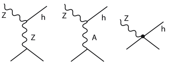
The polarization effect in the cross section arises from the interference of -channel diagrams with and ; see Fig. 1. In addition to the term in the Higgs Lagrangian, the dimension-6 operators in the EFT induce a term
| (6) |
that mixes the and field strengths. The coefficient of this term is related to the parameters already discussed by
| (7) |
This produces the second diagram in Fig. 1, which is not present at tree level in the SM. There is also a third contribution that has the form of a contact interaction. This third diagram is parametrically enhanced by terms of order [25]. However, the EFT coeffiecients that appear in this diagram are very strongly constrained by the analysis of precision electroweak corrections and , in a way that compensates this enhancement [18]. We will ignore this diagram in the simplified analysis presented in this section. However, it does play a role in the more complete analysis that we will describe in Section 4.
The sign of the interference term between the -channel and diagrams depends on the beam polarization. The charge of the electron changes sign between and , (), while the charge stays the same. This leads to a near-cancellation of the terms for , while there is constructive interference for .
To illustrate these effects, we carry out a simplified fit to the Higgs couplings in the following framework: The starting point is the table of projected errors on the total cross section given in the Appendix. These error estimates are based on full simulation studies with the ILD detector model [26, 27]. The estimates are provided for each of two configurations of beam polarization, an beam with electron and positron beam polarizations and an beam with electron and positron beam polarizations . These errors are essentially identical for the two beam polarizations, and so we can apply them also for unpolarized beams. All of the analyses below are carried out at the linearized level.
A fit in the framework would modify each Higgs couplings by
| (8) |
For reference, we carried out a fit to this data from with 7 parameters:
| (9) |
In addition, we allow branching ratios of the Higgs boson to invisible and to non-invisible exotic decay modes. This modification of the Standard Model is usually omitted in EFT fits, which concentrate on the effects of heavy particles. However, the search for Higgs decays to light invisible and exotic particles is an important part of the full program, and the possibility of such decays adds an uncertainty to the extraction of the Higgs boson total width that should be accounted. To parametrize these possible exotic Higgs decays, we introduce two additional parameters and . The parameter is the fraction of all Higgs decays that go to completely invisible decay products,
| (10) |
Similarly, is the fraction of all Higgs decays that do not fit into any standard category, or even into the category of invisible decays. It is extremely conservative to include the parameter, since, at an collider, almost any exotic decay will be observed and recognized as such [28]. But this is the way that all previous “model-independent” Higgs coupling fits for colliders have been done.
The simplified fits in the EFT framework also uses 9 parameters. These are the EFT parameters and , the EFT parameters that shift the Higgs couplings , , , , and , and the and parameters described above (10) [29]. In this simplified fit, and are set equal to zero. In the complete fit described below, these latter parameters are determined by constraints from precision electroweak measurements, , and .
| fit | angl. only | pol. only | both | full EFT fit | |
|---|---|---|---|---|---|
| 3.21 | 3.87 | 0.94 | 0.94 | 1.04 | |
| 3.52 | 4.19 | 1.73 | 1.73 | 1.79 | |
| 3.43 | 4.10 | 1.54 | 1.54 | 1.60 | |
| 3.31 | 3.77 | 0.46 | 0.45 | 0.65 | |
| 3.25 | 3.91 | 1.07 | 1.07 | 1.16 | |
| 0.36 | 3.51 | 0.45 | 0.44 | 0.66 | |
| 13.1 | 14.7 | 12.8 | 12.8 | 5.53 | |
| 0.85 | 0.92 | 0.83 | 0.83 | 0.82 | |
| 3.29 | 0.26 | 0.02 | 0.02 | 0.07 | |
| 6.53 | 7.64 | 2.20 | 2.18 | 2.38 | |
| 0.72 | 0.80 | 0.72 | 0.70 | 0.70 | |
| 0.39 | 0.36 | 0.30 | 0.30 | 0.30 | |
| 1.57 | 1.71 | 1.53 | 1.51 | 1.50 |
The full details of our treatment of the cross section and angular distribution are discussed in [18]. Our approach can be summarized by saying that the perturbations to the SM cross section from the and terms can be completely parametrized in terms of coefficients and , respectively, that describe the variations in the cross section, angular distribution, and polarization. These and parameters depend on beam polarization and center of mass energy. For example, at the tree level, the total cross section for from a fully polarized or initial state is given by
| (11) |
where , are the lab frame momentum and energy of the . In the simplified parameter set used here, the parameters in (11) are given, for a fully polarized initial state, by
| (12) |
and, for a fully polarized initial state, by
| (13) |
The change of sign between the two terms in vs. is the polarization effect described earlier in this section. There are similar formula for the distributions in production angle and decay angles; see [18] for details. Fits for the and parameters using ILD full simulation data are described in [27], and these are the basis for the error estimates and correlations for these parameters listed in the Appendix.
The results of the simplified fits are shown in Table 1. We assume 2000 fb-1 of data, equally divided between the two polarized beam configurations. These fits include only data from . The fit is limited by the poor knowledge of the Higgs total width. In this fit, the width is obtained through the relation (5) and suffers from a lack of statistics for the decay. In the EFT fits, the uncertainty in the couplings reflects the uncertainty in the knowledge of the parameter, which is determined mainly from the data on the reactions . Note that polarization is in general a more powerful analyzer for than the angular distributions, although either method can be effective with a sufficiently large luminosity sample. For reference, the last column of the fit gives the results of the full EFT fit described in the next section. The simplified fit is quite idealized, but its outcome turns out to be close to that of a full EFT analysis.
4 Projections for ILC at 250 GeV
A complete analysis within the EFT framework requires a much larger number of parameters. As stated above, there are 84 possible dimension-6 operators with the gauge symmetry and particle content of the Standard Model. In [18], we point to a subset of 9 of these operators that contribute to processes involving , , Higgs, and light leptons only. Five additional operators modify the Higgs couplings to fermions and gluons. Two further parameters are needed to describe the and couplings to quarks. Then our model-independent fit will involve 16 dimension-6 operator coefficient plus the 4 relevant parameters of the Standard Model and the 2 parameters introduced above for exotic Higgs decays. The total number of parameters is 22. Though many papers have been written about fits to Higgs data using EFT, it seems not to have been realized that data from future colliders will completely constraint these 22 parameters, allowing precise analyses that are model-independent to the extent that this subset of operators gives a general description of new physics.
The subset of 9 operators noted above does not include the most general operators with , , Higgs, and light leptons. It excludes 4-fermion contact interactions, which, however, do not contribute to the observables of relevance here. It assumes muon-electron universality, which can be strongly tested at colliders in decays and in 2-fermion scattering processes. It excludes CP violating operators. But CP violating operators contribute only in order to the observables we consider, and there are other observables linear in these (for example, the forward-backward asymmetry in ) that can bound them at the percent level. It excludes the coefficient that shifts the triple-Higgs coupling, which does not contribute at tree level to the observables we consider here [30]. Some additional qualifications are given Section 2.2 of [18]. Most importantly, our analysis assumes that operators of dimension 8 are negligible and operators of dimension 6 can be treated in linear order only. This makes sense for operators that provide few-percent corrections to the Higgs couplings, corresponding to the sensitivity of future colliders. In this paper, we will treat the dimension 6 operators at the tree level only. If corrections to Higgs couplings turn out to be at the 30% level, one might question this assumption. But unless corrections to the Higgs couplings are very large, our restricted—but still 22-dimensional—parameter set can be considered a model-independent description of new physics for the purpose of Higgs coupling analysis.
The fit parameters are the following: First, since dimension-6 effects renormalize the parameters of the Standard Model, we must include deviations in the 4 Standard Model parameters
| (14) |
In the basis chosen in [18], the 9 EFT parameters for the Higgs and electroweak boson sector are
| (15) |
Of these, the parameters is essentially the parameter of precision electroweak analysis. The parameters , , parametrize current-current interactions between the Higgs boson and the leptons. The parameters , , and parametrize operators quadratic in vector boson field strengths, and parametrizes the one possible operator cubic in the field strength. We need 5 additional coefficients to describe the shifts in the Higgs couplings to fermions and gluons [29],
| (16) |
For our treatment of the Higgs decays to and , we need two further combinations of EFT coefficients, called and in [18], which are measureable from the and boson total widths. Finally, we include the two parameters and introduced above (10).
Given this parameter set, we assume a linear relation between the parameters and observables,
| (17) |
Then measurements of the lead to a covariance matrix for the , which can then be translated into projected errors on Higgs partial widths or Higgs couplings.
As inputs to this process, we take the following information: First, 7 quantities very well measured in precision electroweak studies—, , , , , and —provide 7 strong constraints on the parameter set. Note that we do not need to make any assumption that the electroweak corrections are “oblique” in the sense of [22]. For the and partial widths, we also must input the measured values of the and total widths, as described in [18]. At the level of dimension-6 operators, provides three independent new physics parameters—, , and —that can be constrained by measurement. LEP and LHC measurements already constrain these parameters at the 1% level. For this analysis, we need more than an order of magnitude improvement in the constraints, but we expect that this will be provided by colliders at the same time that they measure the Higgs boson parameters [31]. A projected covariance matrix for these parameters with 2000 fb-1 of data at 250 GeV, estimated from ILD studies of at higher energies by Marchesini [32] and Rosca [33], is given in the Appendix. The LHC experiments will provide a strong measurement of the ratio . The ATLAS analysis [34] estimates the error on this measurement after 3000 fb-1 of data-taking as 3.6-4%. We expect that a measurement strategy dedicated to cancelling systematic errors between these two similar and characteristic processes can reach the statistics limit of 2%. We use this latter number in our fit, but the results are not changed if the error is indeed 4%. This provides the strongest constraint on . The expected LHC measurement of , with an error of 31% [35], also provides a significant constraint on . We also input the expected LHC measurement of [34]. The input values used are listed in the Appendix.
At this stage, the measurements described constrain 13 of the original 22 parameters. This includes all but 2 of the 4+9 parameters relevant to , , Higgs, and light lepton processes. The remaining two free parameters are and , the parameters of the simplified fit described in the previous section. These parameters are constrained by meausurements of the total cross section, angular distribution, and polarization asymmetries in , as explained in the previous section.
The remaining 9 parameters are those that appear only in expressions for the the Higgs boson partial widths. To include these parameters, we add measurements of for followed by Higgs boson decay to specific final states. The decay widths to and also depend on and in a way that put additional constraints on these parameters. This makes the fit for these parameters more robust and decreases its dependence on any particular input.
Though Higgs production through fusion has a small cross section at 250 GeV, we include the measurement of the rate for , .
The full fit contains a number of mechanisms for constraining the and parameters, or, alternatively through (4), the EFT coefficients , , and . We have explained in Section 3 how these parameters are constrained by measurements of . The partial widths for Higgs decay to and also contain these parameters, so measurements of Higgs processes with vector bosons in the final state give constraints. The coefficient is directly constrained by measurements of angular distributions. Linear combinations of the three coefficients give new tree-level contributions to the Higgs decay widths to and , so that the LHC measurements of ratios of branching ratios provide constraints. The effect of the various inputs in determining these coefficients is shown as a systematic progression in Table 2 of [18]. The fact that several different inputs contribute decreases the importance of beam polarization for achieving accurate determinations of the Higgs boson couplings with respect to the results of the simple fits described in Section 3.
On the other hand, there is another effect that must also be accounted. The EFT formalism leads to new contact interactions, of which an example is the third diagram in Fig. 1 [25]. As noted above, these diagrams are enhanced by a factor . They are strongly constrained only when the full set of Higgs processes measurable at colliders is included. The influence of these diagrams, and the role of the inputs in controlling them, is described in some detail in Section 5 of [18].
The results of the full 22-parameter fit are shown in the last column of Table 1. The results are quite similar to those from the simple fit of the previous section. The introduction of many new parameters does not decrease the quality of the fit, since the additional measurements constrain these parameters strongly. The largest effect is seen in the and couplings, where a contribution from adds a small amount to the total error. The full fit also depends much less strongly on beam polarization, since this is now only one of several constraints that determine the parameter . We will see this in the examples presented in the next section.
Table 2 gives a comparison of this EFT fit to previous results that we have presented in the past for ILC, using the framework but including measurements at 500 GeV to sharpen the determination of the Higgs total width. The first column shows the result of this fit. The second and third columns give the results quoted in [3] for the initial and full phases of the ILC program described in [36]. The fourth column shows the results of the fit described in Section 6 of this paper. It is interesting that, with the new analysis method that we present here, a long run at 250 GeV gives considerable power for learning about the Higgs couplings even before we go to higher energy. Eventually, of course, we must do both. Running at 500 GeV and above is also needed to complete the program of precision Higgs measurements by measuring the coupling and the triple Higgs coupling.
| full 250 GeV EFT fit | initial ILC [3] | full ILC [3] | full ILC EFT fit | |
|---|---|---|---|---|
| 1.04 | 1.5 | 0.7 | 0.55 | |
| 1.79 | 2.7 | 1.2 | 1.09 | |
| 1.60 | 2.3 | 1.0 | 0.89 | |
| 0.65 | 0.81 | 0.42 | 0.34 | |
| 1.16 | 1.9 | 0.9 | 0.71 | |
| 0.66 | 0.58 | 0.31 | 0.34 | |
| 5.53 | 20 | 9.2 | 4.95 | |
| 2.38 | 3.8 | 1.8 | 1.50 |
5 Polarization vs. luminosity vs. energy
Beam polarization played an important role in the fits described in Sections 3 and 4. However, as we pointed out in Section 4, inclusion of the full set of observables that can be measured at colliders take some pressure off the requirement for beam polarization. Designs for the proposed circular colliders CEPC and FCC-ee anticipate larger event samples than ILC at 250 GeV, but do not anticipate longitudinally polarized beams. The proposed CLIC linear collider anticipates its initial run at a higher energy of 380 GeV. It is interesting to explore the trade-offs between these proposed programs.
This question can be answered within the EFT formalism by using the data in the Appendix to estimate the inputs for the various accelerator schemes, and then performing a fits analogous to that of Section 4. The results are shown in Table 3. The first column again shows the fit of Section 4, with polarized beams and 2 ab-1 of integrated luminosity. The second column shows the result for the same integrated luminosity at 350 GeV in the center of mass, appropriate for the proposed CLIC linear collider. (The CLIC proposal now considers running at 380 GeV, but all published studies have been done assuming 350 GeV. The CLIC proposal includes additional stages at higher energy that are not considered here [6, 37].) The third and fourth columns show the results for unpolarized beams [38] using the luminosity samples of 5 ab-1, projected for CEPC [5], and for 5 ab-1 at 250 GeV plus 1.5 ab-1 at 350 GeV, approximating the program projected for FCC-ee with 2 detectors [39]. Our error estimates include an accounting for expected systematic errors, as described in the Appendix.
The fifth column shows the results of a fit including data at 500 GeV that will be described in the next section. This fit include 2 ab-1 at 250 GeV plus 4 ab-1 at 500 GeV, realizing the full ILC plan set out in [36].
| 2 ab-1 | 2 ab-1 | 5 ab-1 | + 1.5 ab-1 | full ILC | |
| w. pol. | 350 GeV | no pol. | at 350 GeV | 250+500 GeV | |
| 1.04 | 1.08 | 0.98 | 0.66 | 0.55 | |
| 1.79 | 2.27 | 1.42 | 1.15 | 1.09 | |
| 1.60 | 1.65 | 1.31 | 0.99 | 0.89 | |
| 0.65 | 0.56 | 0.80 | 0.42 | 0.34 | |
| 1.16 | 1.35 | 1.06 | 0.75 | 0.71 | |
| 0.66 | 0.57 | 0.80 | 0.42 | 0.34 | |
| 1.20 | 1.15 | 1.26 | 1.04 | 1.01 | |
| 5.53 | 5.71 | 5.10 | 4.87 | 4.95 | |
| 0.82 | 0.90 | 0.58 | 0.51 | 0.43 | |
| 0.07 | 0.06 | 0.07 | 0.06 | 0.05 | |
| 2.38 | 2.50 | 2.11 | 1.49 | 1.50 | |
| 0.70 | 0.77 | 0.50 | 0.22 | 0.61 | |
| 0.30 | 0.56 | 0.30 | 0.27 | 0.28 | |
| 1.50 | 1.63 | 1.09 | 0.94 | 1.15 |
It is clear from the table that the decreased power of the angular distributions to measure the parameters can be compensated by higher luminosity. One should also remember that the ratios of branching ratios are measured at colliders without ambiguity, and the accuracy of these measurements improves as . These ratios of branching ratios can be important in the testing of specific models, as we will discuss in Section 7.
One should note that beam polarization offers some qualitative advantages that are not captured in a table such as this. Having separate samples with different beam polarization essentially doubles the number of independent observables and allows consistency tests that would be not otherwise be available.
| no pol. | 80%/0% | 80%/30% | |
| 1.33 | 1.13 | 1.04 | |
| 2.09 | 1.97 | 1.79 | |
| 1.90 | 1.77 | 1.60 | |
| 0.98 | 0.68 | 0.65 | |
| 1.45 | 1.27 | 1.16 | |
| 0.97 | 0.69 | 0.66 | |
| 1.38 | 1.22 | 1.20 | |
| 5.67 | 5.64 | 5.53 | |
| 0.91 | 0.91 | 0.82 | |
| 0.07 | 0.07 | 0.07 | |
| 2.93 | 2.60 | 2.38 | |
| 0.78 | 0.78 | 0.70 | |
| 0.36 | 0.33 | 0.30 | |
| 1.68 | 1.67 | 1.50 |
It is amusing to use comparisons such as this one to try to determine the “best” future collider, but truly the best collider is the one that is actually built. The trade-off shown between linear and circular colliders shows that colliders of both types have powerful capability for discovering new physics beyond the Standard Model. We will present an explicit comparison with models for ILC in Section 7. Similar results would be obtained with any of the scenarios shown in Table 3.
It is of some interest to understand the importance of positron polarization, in addition to electron polarization, since positron polarization at linear colliders requires a special type of positron source. Table 4 investigates this question by comparing the results of a complete EFT fit at 250 GeV and 2000 fb-1 for different assumptions about the electron and positron polarization.
6 Inclusion of data at 500 GeV
Our discussion so far has focused mainly on data that might be collected at 250 GeV. The ILC envisions a stage of running at 500 GeV. For CLIC, the current plan is to initially run at 380 GeV, with subsequent stages at 1 TeV and above. Thus it is interesting to consider the effect of higher-energy data on this analysis.
There are three important effects of higher-energy running. First, the fusion process turns on, providing a new source of data on Higgs cross sections and branching ratios. The dependence of this cross section on the parameter is rather weak,
| (18) |
Also, since the Higgs bosons from this reaction are not tagged, it is not possible to directly measure the absolute cross section. However, the fusion cross section is larger than the Higgsstrahlung cross section at 500 GeV, and the luminosity of linear colliders is expected to increase with energy, so this process adds a large amount of information on relative Higgs branching ratios. By combining the cross section measurement to specific final states with absolution branching ratio measurements at 250 GeV, one finds improved constraints on or .
Second, as the center of mass energy increases, the angular distribution of predicted by the Standard Model evolves from one that is relatively flat to a distribution dominated by production of the longitudinal polarization state. Since the contribution of the term is flat in angle and roughly independent of polarization, this allows a much better discrimination of the and contributions than at 250 GeV.
Third, the effects of dimension-6 operators in increases as . Thus, running at higher energy allows stronger constraints on new physics effects in the triple gauge boson couplings, improving the error on the parameter in the manner called for at the end of Section 4.
The results of a complete EFT fit including these effects is shown in the last column of Table 3. This fit assumes 2 ab-1 of data at 250 GeV plus 4 ab-1 at 500 GeV, divided equally between and polarized beams. The input measurements, with accuracies estimated by full simulation with the ILD detector model, are given in the Appendix.
7 Recognition of new physics models
We can use the formalism presented in this paper to give quantitative estimates of the power of measurements of the Higgs boson to discover and discriminate models of new physics beyond the SM. From the large literature on new physics modification of the Higgs couplings, we have chosen a selection of models that we feel are illustrative of possible new physics effects on the Higgs couplings. In this section, we will compare their predictions for Higgs couplings to the ILC error estimates computed in this paper.
The EFT fit presented here can be used to estimate the significance of the observation of Higgs coupling deviations from the SM and discrimination of the effects of different models. Our method makes use of the linear dependence of the Higgs couplings on the EFT coefficients. Consider as observables the Higgs couplings obtained from the fits described in this paper. Each coupling has an expansion in EFT coefficients of the form (17) with coefficients . Let be the Higgs couplings deviations predicted in a given model, arranged as a vector. Let be the covariance matrix of the variables determined by the fit. Then
| (19) |
gives the likelihood testing the goodness of fit for this model relative to the Standard Model. Similarly, if and are two such vectors for models and ,
| (20) |
gives the for given the hypothesis or vice versa. The significance in of the deviation of a model from the SM, or of one model from another, is roughly the square root of the computed in this way.
| Model | |||||||||
|---|---|---|---|---|---|---|---|---|---|
| 1 | MSSM [40] | +4.8 | -0.8 | - 0.8 | -0.2 | +0.4 | -0.5 | +0.1 | +0.3 |
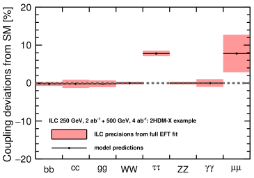
| 2 | Type II 2HD [42] | +10.1 | -0.2 | -0.2 | 0.0 | +9.8 | 0.0 | +0.1 | +9.8 |
| 3 | Type X 2HD [42] | -0.2 | -0.2 | -0.2 | 0.0 | +7.8 | 0.0 | 0.0 | +7.8 |
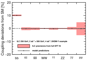
| 4 | Type Y 2HD [42] | +10.1 | -0.2 | -0.2 | 0.0 | -0.2 | 0.0 | 0.1 | -0.2 |
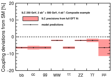
| 5 | Composite Higgs [44] | -6.4 | -6.4 | -6.4 | -2.1 | -6.4 | -2.1 | -2.1 | -6.4 |
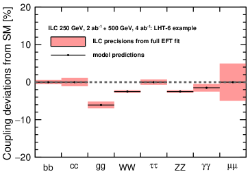
| 6 | Little Higgs w. T-parity [45] | 0.0 | 0.0 | -6.1 | -2.5 | 0.0 | -2.5 | -1.5 | 0.0 |
| 7 | Little Higgs w. T-parity [46] | -7.8 | -4.6 | -3.5 | -1.5 | -7.8 | -1.5 | -1.0 | -7.8 |
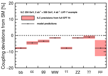
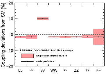
| 8 | Higgs-Radion [47] | -1.5 | - 1.5 | +10. | -1.5 | -1.5 | -1.5 | -1.0 | -1.5 |
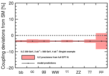
| 9 | Higgs Singlet [48] | -3.5 | -3.5 | -3.5 | -3.5 | -3.5 | -3.5 | -3.5 | -3.5 |
It will always be true that some models of new physics are observable through Higgs coupling deviations while others are not. All viable models of new physics beyond the SM exhibit “decoupling”. That is, as the new particle masses are increased, the predicted deviations from the SM in the Higgs couplings and in other precision observables tend to zero. It is interesting to ask, though, whether there are models that predict significant deviations in the Higgs couplings for parameter values at which the new particles are very heavy, outside the reach of the LHC. A systematic study of supersymmetric models [40, 41] shows that there are a significant number of such models. In fact, Figs. 1–5 of [40] show that constraints on the Higgs couplings proble the model space in a direction roughly orthogonal to that probed by direct particle searches. It makes sense, then, to open this new line of attack on the problem of discovering physics beyond the SM.
To illustrate the range of new physics models that can be found through studies of the Higgs couplings, we present a list of 9 models with significant Higgs boson coupling deviations in which the new particles present in the model are unlikely to be discoverable at the LHC, even in the high-luminosity era. These models are:
-
1.
A supersymmetric model, model #1259073 of the PMSSM models described in [40]. This model has relatively high colored SUSY particle masses: TeV, TeV, but still these shift the coupling significantly. The lightest SUSY particles are a Higgsino multiplet at 515 GeV.
- 2.
- 3.
- 4.
-
5.
A Composite Higgs model MCHM5 with TeV, described in [44]. The lightest new particle in this model is a vectorlike top quark partner at 1.7 TeV. However, the single production cross section for this particle can be very small.
-
6.
A Little Higgs model with T-parity in the family of models considered in [45], with GeV and the top quark partner at 2 TeV. [This model is on the boundary with respect to precision electroweak.]
-
7.
A Little Higgs model with T-parity described in [46], with TeV and the option B for light-quark Yukawa couplings. In this model, the top quark partner has a mass of 2.03 TeV.
-
8.
A Higgs-radion mixing model described in [47]. The radion mass is taken to be 500 GeV; other relevant extra-dimensional states can be at multi-TeV masses.
-
9.
A model with a Higgs singlet is added to the Standard Model to allow electroweak baryogenesis and to provide a portal to the dark matter sector, described in [48]. The singlet mass is 2.8 TeV, with mixing as large as permitted by decoupling.
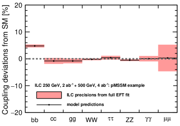
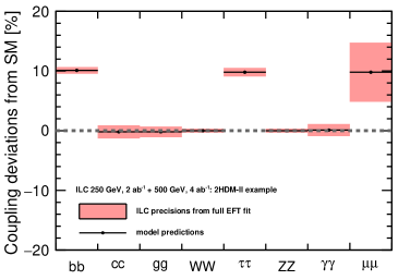
The coupling deviations in these models are listed in Table 5. These deviations are shown graphically in Appendix B, together with the uncertainties that would result from the fit to ILC data at 250 GeV and 500 GeV.
Comparing these models to the Standard Model, we find the following separation. Using the fit of Section 4, for the ILC at 250 GeV with 2 ab-1 of data, the relative s of the models are:
| SM | 1 | 2 | 3 | 4 | 5 | 6 | 7 | 8 | 9 | |
|---|---|---|---|---|---|---|---|---|---|---|
| SM | 0 | 29 | 63 | 43 | 115 | 10 | 12 | 20 | 22 | 7.3 |
| 1 | 29 | 0 | 34 | 113 | 36 | 53 | 24 | 78 | 68 | 37 |
| 2 | 63 | 34 | 0 | 95 | 68 | 105 | 39 | 149 | 120 | 71 |
| 3 | 43 | 113 | 95 | 0 | 256 | 57 | 51 | 71 | 70 | 50 |
| 4 | 115 | 36 | 68 | 256 | 0 | 152 | 97 | 191 | 167 | 123 |
| 5 | 10 | 53 | 105 | 57 | 152 | 0 | 23 | 5.5 | 29 | 8.3 |
| 6 | 12 | 24 | 39 | 51 | 97 | 23 | 0 | 46 | 51 | 8.8 |
| 7 | 20 | 78 | 149 | 71 | 191 | 5.5 | 46 | 0 | 26 | 21 |
| 8 | 22 | 68 | 120 | 70 | 167 | 29 | 51 | 26 | 0 | 23 |
| 9 | 7.3 | 37 | 71 | 50 | 123 | 8.3 | 8.8 | 21 | 23 | 0 |
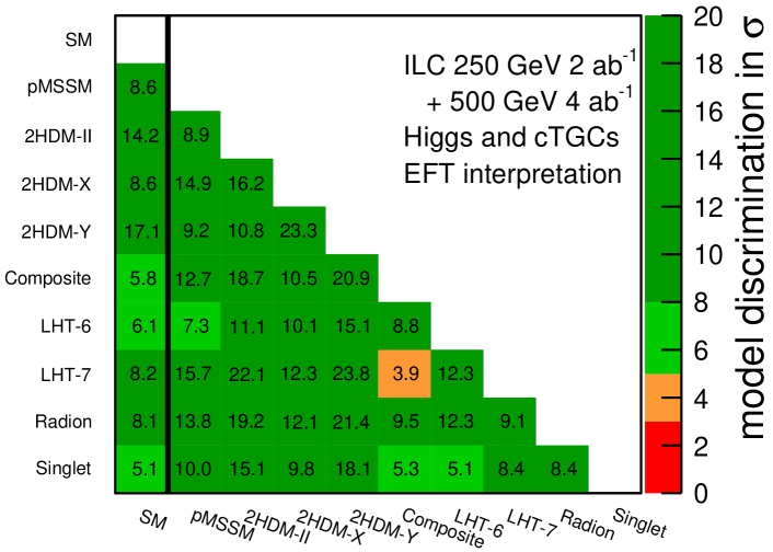
Every model except #9 is separated from the Standard Model by at least 3 , and the models are generally separated from one another by a comparable amount [49]. The separations of the models from the SM and from one another are illustrated in Fig. 2(a).
Using the fit of Section 6, for the ILC at 250 GeV with 2 ab-1 of data and then at 500 GeV with 4 ab-1 of data, the relative s of the models are:
| SM | 1 | 2 | 3 | 4 | 5 | 6 | 7 | 8 | 9 | |
|---|---|---|---|---|---|---|---|---|---|---|
| SM | 0 | 75 | 204 | 75 | 295 | 35 | 39 | 68 | 67 | 27 |
| 1 | 75 | 0 | 80 | 222 | 85 | 162 | 55 | 247 | 193 | 101 |
| 2 | 204 | 80 | 0 | 263 | 118 | 352 | 124 | 492 | 371 | 230 |
| 3 | 75 | 222 | 263 | 0 | 543 | 113 | 104 | 152 | 147 | 97 |
| 4 | 295 | 85 | 118 | 543 | 0 | 438 | 230 | 568 | 458 | 329 |
| 5 | 35 | 162 | 352 | 113 | 438 | 0 | 78 | 17 | 93 | 30 |
| 6 | 39 | 55 | 124 | 104 | 230 | 78 | 0 | 153 | 154 | 27 |
| 7 | 68 | 247 | 492 | 152 | 568 | 17 | 153 | 0 | 85 | 72 |
| 8 | 67 | 193 | 371 | 147 | 458 | 93 | 154 | 85 | 0 | 71 |
| 9 | 27 | 101 | 230 | 97 | 329 | 30 | 27 | 72 | 71 | 0 |
With this data set, the various models are distinguished from the Standard Model at least 5 . Except in two cases, the models are also well distinguished from one another, so that the results give a clear indication of the nature of the new physics that has been discovered through the Higgs coupling deviations. The separations of the models from the SM and from one another are illustrated in Fig. 2(b).
These examples illustrate the ability of future colliders to expose models of new physics even in cases in which the new particles are beyond the reach of direct searches at the LHC.
8 Conclusions
In this paper, we have presented an improved method for the extraction of model-independent Higgs couplings from the data that will be provided by future colliders. We began by explaining that a simple parametrization of new physics effects by rescaling the Standard Model Higgs couplings by parameters is not sufficiently general to encompass the full range of models of new physics. Instead, we advocate the description of new physics effects on Higgs couplings by the coefficients of dimension-6 operators that can be added to the Lagrangian of the Standard Model. This Effective Field Theory description encompasses a broader range of new physics effects. At the same time, it brings in new constraints from gauge invariance and from Higgs cross section measurements not previously considered in fits for Higgs coupling. This method draws information from precision electroweak measurements, , and precision Higgs measurements, thus taking full advantage of the richness of the information provided by future colliders.
Using this approach, we have analyzed the expectations of the ILC and other proposed colliders for extracting the couplings of the Higgs boson with percent-level accuracy and for observing and discriminating models of new physics whose new particles are beyond the reach of LHC. This program gives a powerful avenue to the discovery of physics beyond the Standard Model.
ACKNOWLEDGEMENTS
We benefited very much from discussion of this work with many colleagues, including Halina Abramowicz, Jim Brau, Nathaniel Craig, Erez Etzion, Howard Haber, Sho Iwamoto, Gabriel Lee, Maxim Perelstein, Philipp Roloff, Yael Shadmi, and Tomohiko Tanabe. We are grateful to Christophe Grojean, Ahmed Ismail, Mihoko Nojiri, Maxim Perelstein, and Shinya Kanemura for detailed discussions of the models analyzed in Section 7. We are especially grateful to Gauthier Durieux, Christophe Grojean, Jiayin Gu, and Kechen Wang for sharing with us insights from [14] that were crucial to this work, and for much other useful advice about the application of the EFT formalism. MEP thanks Kirsten Sachs for arranging a visit to DESY that was essential to this collaboration. TB, SJ, and MEP were supported by the US Department of Energy under contract DE–AC02–76SF00515. TB was also supported by a KEK Short-Term Invited Fellowship. He thanks the KEK ILC group for hospitality during this visit. SJ was also supported by the National Research Foundation of Korea under grants 2015R1A4A1042542 and 2017R1D1A1B03030820. KF and TO were supported by the Japan Society for the Promotion of Science (JSPS) under Grants-in-Aid for Science Research 16H02173 and 16H02176. JT was supported by JSPS under Grant-in-Aid 15H02083. RK and JL were supported by the Deutsche Forschungsgemeinschaft (DFG) through the Collaborative Research Centre SFB 676 “Particles, Strings and the Early Universe”, project B1.
Appendix A Error estimates input into the fits presented in this paper
The fits presented in this paper rely on error estimates for precision electroweak, boson, and Higgs boson measurements. In particular, they rely heavily on uncertainties estimated for measurements that can be carried out at the ILC at 250 GeV, 350 GeV and 500 GeV. In this section, we provide tables of the uncertainties we have assumed in the fits preesents here. These uncertainties are based on full-simulation studies done for the SiD and ILD detector models at the ILC and CEPC. We also specify the additional inputs from precision electroweak and LHC measurements of Higgs branching ratios that are used in our analysis.
Table 6 gives the expected statistical errors on Higgs cross section and branching ratio measurements for polarized beams and for luminosity samples of 250 fb-1. The numbers given in Table 6 are statistical errors only. They can be rescaled to any luminosity by dividing by the square root of the integrated luminosity. In our fits, we have added the statistical error of each measurement for Higgs observables ( or ) in quadrature with two types of assumed common systematic errors, from theory prediction, and from luminosity and beam polarizations measurements [33]. For the observables, we have also added in quadrature an additional systematic error from -tagging efficiency, taken to be ( for integrated luminosities in fb-1) [2].
| -80% , +30% | polarization: | |||||
|---|---|---|---|---|---|---|
| 250 GeV | 350 GeV | 500 GeV | ||||
| [50, 51, 52, 53] | 2.0 | 1.8 | 4.2 | |||
| [54, 55] | 0.86 | 1.4 | 3.4 | |||
| [56, 57, 58, 59] | 1.3 | 8.1 | 1.5 | 1.8 | 2.5 | 0.93 |
| [56, 57] | 8.3 | 11 | 19 | 18 | 8.8 | |
| [56, 57] | 7.0 | 8.4 | 7.7 | 15 | 5.8 | |
| [59, 60, 61] | 4.6 | 5.6 ∗ | 5.7 ∗ | 7.7 | 3.4 | |
| [63] | 3.2 | 4.0 ∗ | 16 ∗ | 6.1 | 9.8 | |
| [2] | 18 | 25 ∗ | 20 ∗ | 35 ∗ | 12 ∗ | |
| [64] | 34 ∗ | 39 ∗ | 45 ∗ | 47 | 27 | |
| [65, 66] | 72 ∗ | 87 ∗ | 160 ∗ | 120 ∗ | 100 ∗ | |
| [27] | 7.6 | 2.7 ∗ | 4.0 | |||
| 2.7 | 0.69 ∗ | 0.70 | ||||
| -99.17 | -95.6 ∗ | -84.8 | ||||
| +80% , -30% | polarization: | |||||
| 250 GeV | 350 GeV | 500 GeV | ||||
| 2.0 | 1.8 | 4.2 | ||||
| 0.61 | 1.3 | 2.4 | ||||
| 1.3 | 33 | 1.5 | 7.5 | 2.5 | 3.8 | |
| 8.3 | 11 | 79 | 18 | 36 | ||
| 7.0 | 8.4 | 32 | 15 | 24 | ||
| 4.6 | 5.6 | 24 | 7.7 | 14 | ||
| 3.2 | 4.0 | 66 | 6.1 | 40 | ||
| 18 | 25 | 81 | 35 | 48 | ||
| 34 | 39 | 180 | 47 | 110 | ||
| 72 | 87 | 670 | 120 | 420 | ||
| 9.1 | 3.1 ∗ | 4.2 | ||||
| 3.2 | 0.79 ∗ | 0.75 | ||||
| -99.39 | -96.6 ∗ | -86.5 |
The first two lines of Table 6 give estimates of the expected error in the total cross section and the expected 95% confidence level upper limit on Higgs to invisible decays, assuming the Standard Model predictions. The following entries give the estimated errors on measurements to the given final states, using the reactions and . The uncertainties quoted here are for polarized beams with -80% electron and +30% positron polarization. References to the original studies are given in each line. Most of the estimates in this table are identical to the ones reported in the article “ILC Operating Scenarios” [36], a few of them have been updated since then by new full simulation studies and are briefly described in the following. The estimates for are improved by a factor of 1.4 at GeV, after adding the contributions from channels [61], and by a factor of 1.7 at GeV, after adding the contributions from channels [62]. The estimates for and at GeV are updated based on new analysis performed using ILD DBD simulation and reconstruction tools [58], and, more importantly, the correlation between them, which is , is now incorporated into the fit. The estimates for at GeV are updated based on new full simulation results in [57]. The estimates for are updated to the published results [63]. The up-to-date references for all of the estimates are indicated in the table.
| 250 GeV | 350 GeV | 500 GeV | ||||
|---|---|---|---|---|---|---|
| 0 .062 ∗ | 0.033 ∗ | 0.025 | ||||
| 0.096 ∗ | 0.049 ∗ | 0.034 | ||||
| 0.077 ∗ | 0.047 ∗ | 0.037 | ||||
| 63.4 ∗ | 63.4 ∗ | 63.4 | ||||
| 47.7 ∗ | 47.7 ∗ | 47.7 | ||||
| 35.4 ∗ | 35.4 ∗ | 35.4 |
For the beams with +80% electron and -30% positron polarizations, we generally assume that the expected errors are independent of the polarization state, with a slightly higher cross section for being compensated by slightly lower backgrounds for . Dedicated studies for +80% electron and -30% positron polarization were done for the and measurements, and here we quote the analysis results directly. The fusion process requires the initial state, and so the rate is much smaller in this polarization configuration. The errors quoted in the table are obtained by multiplying the corresponding errors in the top half of the table by 4.1, the inverse of the square root of the relative luminosity.
The errors on the total cross section and angular distribution in are usefully quoted as errors on the and parameters defined in (11) and in [18]. The expected errors on and and their correlation are shown in Table 6. For GeV and 500 GeV, these errors have been estimated in [27] from ILD full-simulation studies for both polarization configurations. For GeV, we have estimated these errors by interpolation.
The expected errors on the anomalous TGC coupling parameters of are shown in Table 7. These errors are based on extrapolation from the studies of [32, 33], taking into account the dependences on , statistics and detector acceptances [67]. Further more, since the studies in [32, 33] are performed using a binned fit for 3 angular distributions in semi-leptonic channel, an additional scaling factor, 1.6-2, is applied to the extrapolations, to take into account the potential improvement from an unbinned fit for 5 angular distributions in both semi-leptonic and full hadronic channels. The errors for TGCs are quoted for samples of 500 fb-1 of data, divided equally between the two polarization states. For simplicity, we use the same estimates for the errors at unpolarized colliders. In our analysis, we have added to these statistical errors the systematic errors for both and , and for [67].
| Observable | current value | current | future | SM best fit value |
|---|---|---|---|---|
| 128.9220 | 0.0178 | (same) | ||
| ( GeV-2) | 1166378.7 | 0.6 | (same) | |
| (MeV) | 80385 | 15 | 5 | 80361 |
| (MeV) | 91187.6 | 2.1 | 91.1880 | |
| (MeV) | 125090 | 240 | 15 | 125110 |
| 0.14696 | 0.0013 | 0.147937 | ||
| (MeV) | 83.984 | 0.086 | 83.995 | |
| (MeV) | 2495.2 | 2.3 | 2.4943 | |
| (MeV) | 2085 | 42 | 2 | 2.0888 |
The precision electroweak inputs to our fit are shown in Table 8. For most of the entries, we have assumed the current uncertainties, from the Particle Data Group compilation [68]. For three of the values, we have assumed improvements in uncertainties: for the mass, from LHC [70], for the Higgs boson mass, from ILC [50], and, for the width, from , using the theoretical value of from our fit and the value of that will be measured at the ILC at 250 GeV with pair events.
We have input the following errors on ratios of branching ratios from the LHC, as described in Section 3:
| (21) |
The full set of linear relations used in this fit, and the final covariance matrices for the fit parameters given by the ILC 250 fit and the full ILC fit are given in files CandV250.txt and CandV500.txt included with the arXiv posting of this paper.
Though we used existing experimental results for the fit, it is worth emphasizing that the fit can benefit from several additional important measurements for which full simulation studies are not yet complete. First, we plan to improve the measurement of at 250 GeV by including contribution from full hadronic channels. Second, we plan to improve the constraints on couplings by adding measurements of the branching ratio for and the cross section for . Third, we plan to improve the constraints on the EFT coefficients , by measuring the cross sections of for both left and right handed beams. Finally, we plan to carry out a full analysis of the meausreement of the branching ratio for which should improve on the estimate given in Table 8.
Appendix B Illustration of the discrimination of models by precision Higgs measurements
Figures 3 and 4 show the deviations from the Standard Model expectations for the Higgs boson couplings, in %, expected for each of the models considered in Section 7, along with the uncertainties that would result from the fit to ILC data at 250 and 500 GeV described in Section 6. Note that these uncertainties are correlated, and that these correlations are taken into account in the values that we quote in Section 7.
References
- [1] H. Baer et al., “The International Linear Collider Technical Design Report - Volume 2: Physics,” arXiv:1306.6352 [hep-ph].
- [2] D. M. Asner et al., “ILC Higgs White Paper,” arXiv:1310.0763 [hep-ph].
- [3] K. Fujii et al., “Physics Case for the International Linear Collider,” arXiv:1506.05992 [hep-ex].
- [4] M. Bicer et al. [TLEP Design Study Working Group], “First Look at the Physics Case of TLEP,” JHEP 1401, 164 (2014) [arXiv:1308.6176 [hep-ex]].
- [5] CEPC-SPPC Study Group, “CEPC-SPPC Preliminary Conceptual Design Report. 1. Physics and Detector,” IHEP-CEPC-DR-2015-01, IHEP-TH-2015-01, IHEP-EP-2015-01.
- [6] H. Abramowicz et al., CLICDP-PUB-2016-001, arXiv:1608.07538v2 [hep-ex].
- [7] R. Lafaye, T. Plehn, M. Rauch, D. Zerwas, and M. Duhrssen, JHEP 0908, 009 (2009) [arXiv:0904.3866 [hep-ph]]; R. Lafaye, T. Plehn, M. Rauch and D. Zerwas, arXiv:1706.02174 [hep-ph].
- [8] G. F. Giudice, C. Grojean, A. Pomarol and R. Rattazzi, JHEP 0706, 045 (2007) [hep-ph/0703164].
- [9] R. Contino, M. Ghezzi, C. Grojean, M. Muhlleitner and M. Spira, JHEP 1307, 035 (2013) [arXiv:1303.3876 [hep-ph]].
- [10] N. Craig, J. Gu, Z. Liu, and K. Wang, JHEP 1603, 050 (2016) [arXiv:1512.06877 [hep-ph]].
- [11] S. F. Ge, H. J. He, and R. Q. Xiao, JHEP 1610, 007 (2016) [arXiv:1603.03385 [hep-ph]].
- [12] J. Ellis, P. Roloff, V. Sanz, and T. You, JHEP 1705, 096 (2017) [arXiv:1701.04804 [hep-ph]].
- [13] H. Khanpour and M. Mohammadi Najafabadi, Phys. Rev. D 95, 055026 (2017) [arXiv:1702.00951 [hep-ph]].
- [14] G. Durieux, C. Grojean, J. Gu, and K. Wang, JHEP 1709, 014 (2017) [arXiv:1704.02333 [hep-ph]].
- [15] S. Di Vita, G. Durieux, C. Grojean, J. Gu, Z. Liu, G. Panico, M. Riembau and T. Vantalon, arXiv:1711.03978 [hep-ph].
- [16] W. H. Chiu, S. C. Leung, T. Liu, K. F. Lyu, and L. T. Wang, arXiv:1711.04046 [hep-ph].
- [17] D. de Florian et al. [LHC Higgs Cross Section Working Group], “Handbook of LHC Higgs Cross Sections: 4. Deciphering the Nature of the Higgs Sector,” arXiv:1610.07922 [hep-ph].
- [18] T. Barklow, K. Fujii, S. Jung, M. E. Peskin, and J. Tian, arXiv:1708.09079 [hep-ph].
- [19] B. Grzadkowski, M. Iskrzynski, M. Misiak, and J. Rosiek, JHEP 1010, 085 (2010) [arXiv:1008.4884 [hep-ph]].
- [20] N. Craig, M. Farina, M. McCullough, and M. Perelstein, JHEP 1503, 146 (2015) [arXiv:1411.0676 [hep-ph]].
- [21] J. Elias-Miró, J. R. Espinosa, E. Masso and A. Pomarol, JHEP 1308, 033 (2013) [arXiv:1302.5661 [hep-ph]].
- [22] M. E. Peskin and T. Takeuchi, Phys. Rev. Lett. 65, 964 (1990), Phys. Rev. D 46, 381 (1992).
- [23] V. Barger, T. Han, P. Langacker, B. McElrath, and P. Zerwas, Phys. Rev. D 67, 115001 (2003) [hep-ph/0301097].
- [24] N. Craig, C. Englert, and M. McCullough, Phys. Rev. Lett. 111, no. 12, 121803 (2013) [arXiv:1305.5251 [hep-ph]].
- [25] J. Cohen, S. Bar-Shalom, and G. Eilam, Phys. Rev. D 94, no. 3, 035030 (2016) [arXiv:1602.01698 [hep-ph]].
- [26] References are given in in J. Tian, presentation at the Asian Linear Collider Workshop 2015, Tsukuba, http://agenda.linearcollider.org/event/6557/. See also the references cited in Appendix A.
- [27] T. Ogawa, “Study of sensitivity to anomalous HVV couiplings at the ILC”, presentation at the EPS Conference on High Energy Physics 2017, Venice, https://indico.cern.ch/event/466934/contributions/2588482/.
- [28] Z. Liu, L. T. Wang, and H. Zhang, Chin. Phys. C 41, no. 6, 063102 (2017) [arXiv:1612.09284 [hep-ph]].
- [29] In the description of Higgs physics by dimension-6 operators, the new physics corrections to the couplings actually depend on two EFT coefficients and , representing the corrections to the loop diagram from corrections to the coupling and from new heavy quarks. These corrections cannot be separated using data from reactions in which the Higgs remains on-shell, so we summarize these effects here in a single parameter called .
- [30] Determination of in this model-independent EFT framework is discussed in [18]. This requires collisions of at least 500 GeV.
- [31] The strong contribution of future measurements to global fits to EFT parameters has been emphasized in J. Ellis and T. You, JHEP 1603, 089 (2016) [arXiv:1510.04561 [hep-ph]].
- [32] I. Marchesini, “Triple gauge couplings and polarization at the ILC and leakage in a highly granular calorimeter,” DESY-THESIS-2011-044.
- [33] A. Rosca, “Measurement of the charged triple gauge boson couplings at the ILC,” Nucl. Part. Phys. Proc. 273-275, 2226 (2016).
- [34] ATLAS Collaboration, “Projections for measurements of Higgs boson signal strengths and coupling parameters with the ATLAS detector at a HL-LHC”, ATL-PHYS-PUB-2014-016 (2014).
- [35] ATLAS Collaboration, ATL-PHYS-PUB-2014-006 (2014).
- [36] J. E. Brau et al. [ILC Parameters Joint Working Group], “500 GeV ILC Operating Scenarios,” arXiv:1506.07830 [hep-ex].
- [37] The actual program presented in [6] would take only 500 fb-1 of data a 380 GeV and then upgrade to a center of mass energy of 1.4 TeV. One might question the validity of an EFT analysis at 1.4 TeV, and we have not studied this issue sufficienty. We hope that the comparison shown in Table 3 is sufficiently informative.
- [38] The errors estimated in the Appendix for the new physics parameters in make use of the polarization asymmetry, among other observables. For simplicity, we input the same errors in our fits for unpolarized colliders.
- [39] P. Janot, presentation at the FCC Week 2017, indico.cern.ch/event/556692/.
- [40] M. Cahill-Rowley, J. Hewett, A. Ismail, and T. Rizzo, arXiv:1308.0297 [hep-ph].
- [41] M. Cahill-Rowley, J. Hewett, A. Ismail, and T. Rizzo, Phys. Rev. D 90, no. 9, 095017 (2014) [arXiv:1407.7021 [hep-ph]].
- [42] S. Kanemura, H. Yokoya, and Y. J. Zheng, Nucl. Phys. B 886, 524 (2014) [arXiv:1404.5835 [hep-ph]].
- [43] S. Kanemura, M. Kikuchi, K. Sakurai, and K. Yagyu, arXiv:1705.05399 [hep-ph].
- [44] R. Contino, L. Da Rold, and A. Pomarol, Phys. Rev. D 75, 055014 (2007) [hep-ph/0612048].
- [45] J. Hubisz, P. Meade, A. Noble, and M. Perelstein, JHEP 0601, 135 (2006) [hep-ph/0506042].
- [46] C. R. Chen, K. Tobe, and C.-P. Yuan, Phys. Lett. B 640, 263 (2006) doi:10.1016/j.physletb.2006.07.053 [hep-ph/0602211].
- [47] J. L. Hewett and T. G. Rizzo, JHEP 0308, 028 (2003) [hep-ph/0202155].
- [48] S. Di Vita, C. Grojean, G. Panico, M. Riembau and T. Vantalon, arXiv:1704.01953 [hep-ph].
- [49] Technically, we convert the for model A given model B to a -value, then quote this as a number of s for a 1-degree-of freedom comparison. The result is very close to .
- [50] J. Yan, S. Watanuki, K. Fujii, A. Ishikawa, D. Jeans, J. Strube, J. Tian, and H. Yamamoto, Phys. Rev. D 94, no. 11, 113002 (2016) [arXiv:1604.07524 [hep-ex]].
- [51] T. Tomita, “Hadronic Higgs Recoil Mass Study with ILD at 250GeV”, presentation at Asian Linear Collider Workshop, KEK, Tsukuba, Japan, April 19-24, 2015, http://agenda.linearcollider.org/event/6557/session/1/contribution/99
- [52] M. Thomson, Eur. Phys. J. C 76, no. 2, 72 (2016) [arXiv:1509.02853 [hep-ex]].
- [53] A. Miyamoto, arXiv:1311.2248 [hep-ex].
- [54] A. Ishikawa, “Search for invisible Higgs decays at the ILC”, presentation at Linear Collider Workshop, Belgrade, Serbia, October 5-10, 2014, http://agenda.linearcollider.org/event/6389/session/0/contribution/140
- [55] J. Tian, “Higgs Projections”, presentation at Asian Linear Collider Workshop, KEK, Tsukuba, Japan, April 19-24, 2015, https://agenda.linearcollider.org/event/6557/session/12/contribution/129
- [56] H. Ono and A. Miyamoto, Eur. Phys. J. C 73, no. 3, 2343 (2013) doi:10.1140/epjc/s10052-013-2343-8 [arXiv:1207.0300 [hep-ex]].
- [57] F. J. Müller, doi:10.3204/PUBDB-2016-02659 (2016).
- [58] J. Tian, “Update of analysis”, presentation at ILD Analysis and Software Meeting on July 19, 2017, https://agenda.linearcollider.org/event/7703/contributions/39487/attachments/31909/48179
- [59] C. Duerig, K. Fujii, J. List and J. Tian, arXiv:1403.7734 [hep-ex].
- [60] H. Ono, “Higgs Branching Fraction Study”, presentation at the KILC2012 workshop, April 2012, https://agenda.linearcollider.org/event/5414/contributions/23402.
- [61] L. Liao, “Study of BR() at CEPC”, presentation at The 51st General Meeting of ILC Physics Subgroup, April 15, 2017, https://agenda.linearcollider.org/event/7617.
- [62] M. Pandurovic, “Measurement of the decay at 500 GeV ILD and at 3 TeV CLIC”, presentation at the International Workshop on Linear Colliders (LCWS16), Morioka, Dec. 2016, https://agenda.linearcollider.org/event/7371/contributions/37896/.
- [63] S. i. Kawada, K. Fujii, T. Suehara, T. Takahashi, and T. Tanabe, Eur. Phys. J. C 75, no. 12, 617 (2015) doi:10.1140/epjc/s10052-015-3854-2 [arXiv:1509.01885 [hep-ex]].
- [64] C. Calancha, “Full simulation study on H-¿gamma gamma with the ILD detector”, presentation at Linear Collider Workshop 2013, , Tokyo, http://agenda.linearcollider.org/event/6000/session/31/contribution/180.
- [65] H. Aihara, P. Burrows, M. Oreglia, et al., “SiD Letter of Intent”, arXiv:0911.0006, SLAC-R-944 (2009).
- [66] C. Calancha, “Study of Higgs to at 1 TeV at the ILC”, LC-REP-2013-006 (2013).
- [67] R. Karl, “Prospects for electroweak precision measurements and triple gauge couplings at a staged ILC”, presentation at the EPS Conference on High Energy Physics 2017, Venice, https://indico.cern.ch/event/466934/contributions/2589875/.
- [68] J. Erler and A. Freitas, in C. Patrignani et al. (Particle Data Group), Review of Particle Physics, Chin. Phys. C 40, 100001 (2016).
- [69] S. Schael et al., Phys. Rept. 427, 257 (2006) [hep-ex/0509008].
- [70] A. Kotwal, et al., in in the Proceedings of the APS DPF Community Summer Study (Snowmass 2013), N. Graf, J. L. Rosner, and M. E. Peskin, eds., http://www.slac.stanford.edu/econf/C1307292/, arXiv:1310.6708 [hep-ph].