Impact of non-stationarity on hybrid ensemble filters: A study with a doubly stochastic advection-diffusion-decay model

Abstract

Effects of non-stationarity on the performance of hybrid ensemble filters are studied (by hybrid filters we mean those which blend ensemble covariances with some other regularizing covariances). To isolate effects of non-stationarity from effects due to nonlinearity (and the non-Gaussianity it causes), a new doubly stochastic advection-diffusion-decay model (DSADM) is proposed. The model is hierarchical: it is a linear stochastic partial differential equation whose coefficients are random fields defined through their own stochastic partial differential equations. DSADM generates conditionally Gaussian spatiotemporal random fields with a tunable degree of non-stationarity in space and time. DSADM allows the use of the exact Kalman filter as a baseline benchmark.

In numerical experiments with DSADM as the “model of truth”, the relative importance of the three kinds of covariance blending is studied: with static, time-smoothed, and space-smoothed covariances. It is shown that the stronger the non-stationarity, the less useful the static covariance matrix becomes and the more beneficial the time-smoothed covariances are. Time-smoothing of background-error covariances proved to be systematically more useful than their space-smoothing. Under non-stationarity, a filter that extends the (previously proposed by the authors) Hierarchical Bayes Ensemble Filter and accommodates the three covariance-blending techniques is shown to outperform all other configurations of the filters tested. The R code of the model and the filters is available from github.com/cyrulnic/NoStRa.

[figure]style=plain,subcapbesideposition=top

Keywords: Non-stationary spatiotemporal random field, Hierarchical modeling, Advection-diffusion-decay model, EnKF, Hybrid ensemble filters, Hierarchical Bayes Ensemble Filter, Data assimilation.

Running head: Impact of non-stationarity on hybrid filters

1 Introduction

Ensemble Kalman filters (EnKF) estimate background-error covariances from an ensemble of forecasts. The resulting sample covariances are noisy and rank deficient if the ensemble size is not greater than the dimensionality of the covariance matrix (which is typically the case in geosciences). A kind of regularization (that is, introduction of additional information to stabilize the solution) is needed to make them a useful estimate of true background-error covariances. Two regularization techniques are most popular: localization and hybridization. Our focus in this study is on the second technique, in which sample covariances are blended (mixed) with some regularizing covariances and which we therefore call “covariance blending”.

From the literature, we can identify three main types of covariance blending. First, hybrid ensemble-variational filters (EnVar) employ blending with static “climatological” covariances [18, 24, 12]. In statistical literature this regularization device is known as a shrinkage estimator [22]. Second, in the Hierarchical Bayes Ensemble Filter (HBEF) by Tsyrulnikov & Rakitko [43], ensemble covariances are blended with time-smoothed recent-past covariances. The idea of accommodating recent-past background-error statistics has also been explored by other authors: Gustafsson et al. [17] use time-lagged ensemble members, Berre et al. [6] use ensemble members from past 4 days to increase the ensemble size, Bonavita et al. [10] use ensemble covariances from previous 12 days to estimate their parametric covariance model, Lorenc [25] found that using time-lagged and time-shifted perturbations increases the effective ensemble size. Third, Buehner & Charron [11], Ménétrier et al. [30], Ménétrier & Auligné [29] studied spatial smoothing of ensemble covariances, which also can be considered as covariance blending, this time with neighboring covariances in space.

With any of the above kinds of covariance blending, the intention is to reduce sampling noise and increase the rank of the covariance matrix — but at the expense of reducing flow dependence (the main advantage of ensemble statistics) in the blended covariances. The question arises: what are the optimal weights of the regularizing covariances in the blend and which factors do they depend on?

First of all, we notice that if a data assimilation system is stationary, that is, its true (actual) spatial error covariances do not change in time, then there is no need for an (on-line) ensemble at all. Indeed, with constant-in-time background-error covariances, all one has to do is to carefully estimate (off-line) their spatial covariance matrix (through temporal averaging of innovation-based or ensemble covariances). In the Gaussian case, the estimated static covariance matrix will be optimal [see, e.g., Theorem 2.38 in 21, for a formal statement]. Thus, we conclude that only under non-stationarity ensemble filters can outperform data assimilation schemes that employ static background-error covariances. True background-error covariances in a data assimilation scheme are non-stationary either if the system is governed by a non-stationary model or the observation network is changing in time (or both, of course). In this research, our focus is on non-stationarity caused by the model. To study the impact of non-stationarity on the optimal design of hybrid filters we seek a toy model that is capable of producing spatiotemporal fields with tunable non-stationarity.

Most toy models used in data assimilation studies are nonlinear. The simplest models have just a few variables, like the Ikeda model [19], the double well model [31], and the most popular three-variable Lorenz’63 model [26]. Models defined on a 1D spatial domain include, among others, the viscous Burgers equation [2], the Korteweg–de Vries equation [32], and the most popular Lorenz’96 and Lorenz’2005 models [28, 27]. In nonlinear models, the tangent-linear model operator, generally, varies in time, giving rise to non-stationarity (flow-dependence) of filtering probability distributions. However, with nonlinear models, non-stationarity is inevitably intertwined with nonlinearity of the evolution of filtering errors and their ensuing non-Gaussianity. To disentangle effects due to nonlinearity from effects of non-stationarity, we propose a model that gives rise to non-stationary filtering distributions while being linear and Gaussian.

We build the model on the time-discrete scalar (i.e., one-variable) model introduced by Tsyrulnikov & Rakitko [43]:

$$\xi_{k}=F_{k}\xi_{k-1}+\sigma_{k}\alpha_{k},$$ (1)

where $\xi_{k}$ is the (scalar) true system state, $k$ labels the time instant, $F_{k}$ is the (scalar) model operator, $\sigma_{k}$ is the standard deviation of the forcing, and $\alpha_{k}\sim{\cal N}(0,1)$ is the driving white noise. The model is doubly stochastic [e.g. 39], which means that not only the forcing $\alpha_{k}$ is random, the coefficients $F_{k}$ and ${\sigma}_{k}$ are random sequences by themselves, each defined through its own stochastic model similar to Eq.(1) but with a constant model operator and constant magnitude of the forcing. Conditionally on the processes $F_{k}$ and ${\sigma}_{k}$ (that is, after their realizations are computed and kept fixed), Eq.(1) is a linear model with time-varying coefficients [e.g. 13, Section 11.2.1], whose solution is a non-stationary random process. In this study we extend the model Eq.(1) to the spatiotemporal context. The result is a new doubly stochastic advection-diffusion-decay model (DSADM), whose solutions are non-stationary conditionally Gaussian random fields.

The general idea of non-stationary random field modeling by assuming that parameters of a spatial or spatiotemporal model are random fields themselves is discussed by several authors. Piterbarg & Ostrovskii [35] study an advection-diffusion model whose coefficients are random fields with prescribed covariance functions. Lindgren et al. [23] allow a length-scale parameter and a variance parameter of their stochastic partial differential equation to slowly vary in space (by expanding them in a set of basis functions). Banerjee et al. [5, sec. 11.6] mention the possibility of formulating a stochastic differential equation for parameters of another stochastic differential equation. Roininen et al. [36] use a stochastic elliptic equation to model a spatial random field and introduce a hypermodel for its local length scale to achieve non-stationarity; the hypermodel employs the same stochastic elliptic equation. Dunlop et al. [14] discuss (among others) more general Gaussian hierarchical processes, which are defined through a hierarchy of levels so that at each level, the conditional probability distribution is Gaussian given the previous (parent) level. Our innovation is the non-stationary hierarchical model with spatiotemporal stochastic partial differential equations at two levels in the hierarchy. The particular pattern of the non-stationarity (that is, how the field’s variance, local space and time scales, etc. vary in space-time) is random, and its spatiotemporal structure is highly tunable by the model’s hyperparameters.

The rest of the paper is organized as follows. In sections 2–5 we motivate, describe, and examine in numerical experiments the new DSADM model. In section 6 we introduce a new hybrid-HBEF (named HHBEF) filter, which accommodates the three covariance-blending techniques mentioned above. In section 7 we present results of numerical experiments with hybrid ensemble filters showing the crucial impact of non-stationarity on the filters’ performance and optimal design. Efficient numerical implementation of hybrid filters is beyond the scope of this study.

The R code of the doubly stochastic model, the filters, and the R scripts that produced this paper’s numerical results are available from https://github.com/cyrulnic/NoStRa. More detailed texts on the DSADM’s numerical scheme, generation of initial conditions, specification of model parameters, etc. can also be found there.

2 Stochastic advection-diffusion-decay model with constant coefficients

To introduce notation and motivate the new doubly stochastic advection-diffusion-decay model, we theoretically examine here statistics of solutions to a stationary stochastic advection-diffusion-decay model with non-stochastic and constant coefficients (parameters). Specifically, we identify how the model parameters affect the variance, the spatial scale, and the time scale of the solution. This is a preparatory section with largely background material.

2.1 Model

The model is the following stochastic partial differential equation (Whittle [44, Ch. 20, Sec. 3], Lindgren et al. [23, Eq.(17)], Sigrist et al. [38]):

$$\frac{\partial\xi}{\partial t}+U\frac{\partial\xi}{\partial s}+\rho\xi-\nu\frac{\partial^{2}\xi}{\partial s^{2}}=\sigma\alpha,$$ (2)

where $t$ is time, $s$ is the spatial coordinate on the circle ${\mathbb{S}}^{1}(R)$ of radius $R$, $U$ is the advection velocity, $\rho$ is the decay (damping) parameter, $\nu$ is the diffusion parameter, $\alpha(t,s)$ is the standard white (in space and time) Gaussian noise, and $\sigma$ is the intensity of the forcing. The four parameters $\boldsymbol{\theta}=(U,\rho,\nu,\sigma)$ are constant in space and time.

2.2 Stationary spatiotemporal statistics

We start with rewriting Eq.(2) using the material time derivative (i.e., along the characteristic $s=s_{0}+Ut$), or, equivalently, switching to the Lagrangian frame of reference by making the change of variables $(t,s)\mapsto(t,s-Ut)$:

$$\frac{{\rm d}\xi}{{\rm d}t}+\rho\xi-\nu\frac{\partial^{2}\xi}{\partial s^{2}}=\sigma\alpha.$$ (3)

Next, we employ the spectral expansion in space (retaining only those spectral components that are resolved on the regular spatial grid with $n$ points),

$$\xi(t,s)=\sum_{m=-n/2+1}^{n/2}\tilde{\xi}_{m}(t)\,\mathrm{e}^{\mathsf{i}{ms}/{R}}$$ (4)

and

$$\alpha(t,s)=\sum_{m=-n/2+1}^{n/2}\tilde{\alpha}_{m}(t)\,\mathrm{e}^{\mathsf{i}{ms}/{R}},$$ (5)

where $\mathsf{i}$ is the imaginary unit and $\tilde{\xi}_{m}(t)$ and $\tilde{\alpha}_{m}(t)$ are the (complex) spectral coefficients. It can be shown [e.g. 41, Appendix A.4] that $\tilde{\alpha}_{m}(t)$ are independent standard complex-white-noise processes $\omega_{m}(t)$ with the common intensity $a={1}/{\sqrt{2\pi R}}$:

$$\tilde{\alpha}_{m}(t)=a\,\omega_{m}(t).$$ (6)

Now, we substitute Eqs.(4)–(6) into Eq.(3), getting

$$\frac{{\rm d}\tilde{\xi}_{m}}{{\rm d}t}+(\rho+\frac{\nu}{R^{2}}m^{2})\tilde{\xi}_{m}=a\sigma\omega_{m}(t).$$ (7)

This is the spectral-space form of the model Eq.(3). It is easily seen that if $\rho+\frac{\nu}{R^{2}}m^{2}>0$, the solutions to Eq.(7) for different $m$ become, after an initial transient, mutually independent stationary zero-mean random processes.

This implies that the physical-space solution $\xi(t,s)$ becomes a zero-mean random field that is stationary in time and space. Note that by definition, the zero-mean real-valued random field (process) $\xi(t,s)$ is (second-order) stationary if its spatiotemporal covariance function $\gamma(t_{1},s_{1};\,t_{2},s_{2})=\operatorname{\mathbb{E}}\xi(t_{1},s_{1})\,{\xi(t_{2},s_{2})}$ is invariant under translations: $\operatorname{\mathbb{E}}\xi(t_{1},s_{1})\,\xi(t_{2},s_{2})=\operatorname{\mathbb{E}}\xi(t_{1}+u,s_{1}+v)\,\xi(t_{2}+u,s_{2}+v)$ and thus is a function of the space and time shifts only: $\gamma(t,s)=\operatorname{\mathbb{E}}\xi(t_{1},s_{1})\,{\xi(t_{1}+t,s_{1}+s)}$. Here periodicity in the spatial coordinate $s$ is of course assumed, $\xi(t,s)=\xi(t,s+2\pi R)$.

Each elementary stochastic process $\tilde{\xi}_{m}(t)$ is an Ornstein-Uhlenbeck process [e.g. 3, sec. 8.3] with the stationary covariance function

$$B_{m}(t)=b_{m}\cdot\mathrm{e}^{-{|\mathnormal{t}|}/\mathnormal{\tau_{m}}},$$ (8)

where the spectral variances $b_{m}$ are

$$b_{m}=\frac{a^{2}\sigma^{2}}{2}\cdot\frac{1}{\rho+\frac{\nu}{R^{2}}m^{2}}$$ (9)

and the spectral time scales $\tau_{m}$ are

$$\tau_{m}=\frac{1}{\rho+\frac{\nu}{R^{2}}m^{2}}.$$ (10)

Note that Eq.(10) provides the motivation for the inclusion of the decay term in the model. Indeed, with $\rho=0$, the time scale $\tau_{0}$ would be infinitely large, which, on the finite sphere, is unphysical (specifying $b_{0}=0$ could resolve the problem but only at the expense of nullifying $\tilde{\xi}_{0}$, which is also unphysical).

The stationary in space-time covariance function $\gamma(t,s)$ of the random field $\xi(t,s)$ can be easily derived from Eq.(4) while utilizing the independence of the spectral processes $\tilde{\xi}_{m}(t)$, the spectral-space temporal covariance functions given in Eq.(8), and returning to the Eulerian frame of reference:

$$\gamma(t,s)=\sum_{m=-n/2+1}^{n/2}b_{m}\,\mathrm{e}^{-{|\mathnormal{t}|}/\mathnormal{\tau_{m}}}\,\mathrm{e}^{\mathsf{i}\mathnormal{m{(s-Ut)}/R}}.$$ (11)

Note that Eq.(11) implies that the space-time correlations are non-separable, i.e., they cannot be represented as a product of purely spatial and purely temporal correlations. Moreover, according to Eq.(10), smaller spatial scales (i.e., larger wavenumbers $m$) correspond to smaller time scales $\tau_{m}$. This feature of space-time correlations (“proportionality of scales”) is physically reasonable—as opposed to the simplistic and unrealistic separability of space-time correlations—and widespread in the real world, see Tsyroulnikov [40], Tsyrulnikov & Gayfulin [42] and references therein.

Finally, from Eq.(11), the stationary (steady-state) variance of $\xi(t,s)$ is

$${\mathsf{Var}}\,\xi\equiv(\operatorname{SD}(\xi))^{2}=\sum_{m=-n/2+1}^{n/2}b_{m}=\frac{a^{2}\sigma^{2}}{2}\sum_{m=-n/2+1}^{n/2}\frac{1}{\rho+\frac{\nu}{R^{2}}m^{2}},$$ (12)

where $\operatorname{SD}$ stands for standard deviation.

2.3 Roles of model parameters

Firstly, we note that $U$ does not impact the variance spectrum and the spectral time scales of $\xi$ (see Eqs.(9) and (10)), its role is just to rotate the solution with the constant angular velocity $U/R$.

Secondly, Eq.(9) implies that the shape of the spatial spectrum is

$$b_{m}\propto\frac{1}{\rho+\frac{\nu}{R^{2}}m^{2}}\propto\frac{1}{1+(\frac{m}{m_{0}})^{2}},$$ (13)

where $m_{0}=R\sqrt{{\rho}/{\nu}}$ is the characteristic non-dimensional wavenumber, which defines the width of the spectrum and thus the field’s length scale. Therefore, the latter can be defined as the inverse dimensional wavenumber $m_{0}/R$:

$$L=\sqrt{\frac{\nu}{\rho}}.$$ (14)

Thus, the ratio ${\nu}/{\rho}$ controls the length scale $L$. In addition, ${\nu}/{\rho}$ impacts the temporal correlations. Indeed, a higher $L$ implies a redistribution of the variance towards larger spatial scales (i.e., lower wavenumbers $m$). But as we noted, in the model Eq.(2), larger spatial scales correspond to larger time scales $\tau_{m}$. As a result, a higher ${\nu}/{\rho}$ leads to a larger time scale as well as the length scale $L$.

Thirdly, using Eq.(14), we can rewrite Eq.(10) as

$$\tau_{m}=\frac{1}{\rho}\cdot\frac{1}{1+(\frac{Lm}{R})^{2}}$$ (15)

This equation implies that with $L$ being fixed, all spectral time scales $\tau_{m}$ are inversely proportional to $\rho$, which, thus, determines the physical-space Lagrangian time scale $T$ of the spatiotemporal random field $\xi$. We define $T$ as the macroscale [e.g. 46, Eq.(2.88)] along the characteristic,

$$T=\frac{1}{2{\mathsf{Var}}\,\xi}\int_{-\infty}^{\infty}\gamma(t,Ut){\rm d}t=\frac{\sum b_{m}\tau_{m}}{\sum b_{m}}=\frac{1}{\rho}\,\frac{\sum[1+(\frac{Lm}{R})^{2}]^{-2}}{\sum[1+(\frac{Lm}{R})^{2}]^{-1}},$$ (16)

where the second equality is due to Eq.(11), the third equality is due to Eqs.(9) and (15), and the summations are over $m$ from $-\frac{n}{2}+1$ to $\frac{n}{2}$.

Technically, Eqs.(14), (16), and (12) allow us to compute the internal model parameters $\rho$, $\nu$, and $\sigma$ from the externally specified parameters $L$, $T$, and $\operatorname{SD}(\xi)$. Conceptually, we summarize the above conclusions as follows.

• $U$ does not affect the Lagrangian spatiotemporal covariances. It tilts the Eulerian spatiotemporal correlations towards the direction ${\rm d}s=U{\rm d}t$ in space-time.

• The ratio ${\nu}/\rho$ determines the spatial scale $L$ and impacts the time scale $T$.

• With the ratio ${\nu}/\rho$ being fixed, $\rho$ controls the time scale $T$.

• With $\rho$ and $\nu$ being fixed, $\sigma$ determines the resulting process variance ${\mathsf{Var}}\,\xi$.

These conclusions give us an idea how local properties of the spatiotemporal field statistics are going to be impacted if the parameters $\boldsymbol{\theta}=(U,\rho,\nu,\sigma)$ become variable in space and time.

3 Doubly stochastic advection-diffusion-decay model (DSADM)

Here, we allow the parameters $\boldsymbol{\theta}=(U,\rho,\nu,\sigma)$ of the model Eq.(2) to be spatiotemporal random fields by themselves. The resulting model becomes, thus, a three-level hierarchical model [45, 5]. At the first level is the random field in question $\xi(t,s)$ modeled conditionally on the second-level fields $\boldsymbol{\theta}(t,s)=(U(t,s),\rho(t,s),\nu(t,s),\sigma(t,s))$, which are controlled by the third-level hyperparameters $\boldsymbol{\phi}$. So, to compute a realization of the pseudo-random field $\xi(t,s)$, we first specify the hyperparameters $\boldsymbol{\phi}$. Then, we compute realizations of the second-level (secondary or parameter) fields $\boldsymbol{\theta}(t,s)$. Finally, we substitute the secondary fields for the respective parameters in Eq.(2) and solve the resulting equation for the primary field $\xi(t,s)$.

The idea behind this extension of the basic model Eq.(2) is the following. If the secondary fields $\boldsymbol{\theta}(t,s)$ vary smoothly in space and time, then, locally, in a vicinity of some point in space-time $(t_{0},s_{0})$, the statistics of the field $\xi(t,s)$ will resemble that for the stationary model Eq.(2) with constant parameters equal to $\boldsymbol{\theta}(t,s)$ frozen at the point $(t_{0},s_{0})$ [see also 23, sec. 3.2]. As the statistics of the model Eq.(2) with constant parameters do depend on the parameters $\boldsymbol{\theta}$ (see section 2), the resulting solution $\xi(t,s)$ to the model Eq.(2) with variable parameters becomes non-stationary in space-time, with the degree of the non-stationarity controlled by the variability in the secondary fields $\boldsymbol{\theta}(t,s)$.

3.1 First level of the hierarchy: the field in question $\xi$

At the first level, $\xi(t,s)$ satisfies the basic Eq.(2) with variable in space and time coefficients,

$$\frac{\partial\xi}{\partial t}+U(t,s)\,\frac{\partial\xi}{\partial s}+\rho(t,s)\,\xi-\nu(t,s)\,\frac{\partial^{2}\xi}{\partial s^{2}}=\sigma(t,s)\,\alpha(t,s).$$ (17)

3.2 Second level of the hierarchy: parameter fields $\boldsymbol{\theta}$

Each secondary field $\theta(t,s)$ (that is, one of the coefficients $U(t,s)$, $\rho(t,s)$, $\nu(t,s)$, $\sigma(t,s)$ of the first-level Eq.(17)) is modeled as the transformed Gaussian field: $\theta=g_{\theta}(\theta^{*},\boldsymbol{\phi})$. Here $g_{\theta}$ is the (secondary-field specific) transformation function and $\theta^{*}(t,s)$ is the pre-transform Gaussian random field satisfying its own stochastic advection-diffusion-decay model Eq.(2) with constant and non-random coefficients, $U_{\theta},\rho_{\theta},\nu_{\theta},\sigma_{\theta}$ (which are hyperparameters).

The pointwise transformation $g_{\theta}:\theta^{*}(t,s)\mapsto\theta(t,s)$ is specified to be linear for $U$ and nonlinear for the other three parameter fields. The transformation function involves additional hyperparameters: the “unperturbed” value of $\theta$ (a scalar) denoted by the overbar, $\overline{\theta}$ (such that $\theta(t,s)=\overline{\theta}$ if ${\mathsf{Var}}\,\theta^{*}=0$), and a few additional hyperparameters as described below.

Since the pre-transform fields $\theta^{*}(t,s)$ are governed by the models with constant coefficients, $\theta^{*}(t,s)$ are stationary in space-time. The transforms $g_{\theta}$ are defined to be independent of $(t,s)$, therefore the secondary fields $\theta(t,s)$ are stationary in space-time, too.

Next, the computation of the four secondary fields is described, including equations for the pre-transform random fields and the respective transformation functions.

3.2.1 $U(t,s)$

The pre-transform Gaussian field $U^{*}(t,s)$ satisfies the basic stochastic model Eq.(2):

$$\frac{\partial U^{*}}{\partial t}+U_{U}\frac{\partial U^{*}}{\partial s}+\rho_{U}U^{*}-\nu_{U}\frac{\partial^{2}U^{*}}{\partial s^{2}}=\sigma_{U}\,\alpha_{U}(t,s),$$ (18)

where $U_{U},\rho_{U},\nu_{U}$, and $\sigma_{U}$ are constant and non-random hyperparameters and $\alpha_{U}$ is the white noise independent of $\alpha$. The transformation $U^{*}(t,s)\mapsto U(t,s)$ is simply

$$U(t,s)=\overline{U}+U^{*}(t,s),$$ (19)

where $\overline{U}$ is the unperturbed value of $U$ (a non-random scalar).

From linearity of Eqs.(18) and (19), $U(t,s)$ is a Gaussian random field.

3.2.2 $\sigma(t,s)$

The pre-transform Gaussian field $\sigma^{*}(t,s)$ satisfies

$$\frac{\partial\sigma^{*}}{\partial t}+U_{\sigma}\frac{\partial\sigma^{*}}{\partial s}+\rho_{\sigma}\sigma^{*}-\nu_{\sigma}\frac{\partial^{2}\sigma^{*}}{\partial s^{2}}=\sigma_{\sigma}\,\alpha_{\sigma}(t,s).$$ (20)

where $U_{\sigma},\rho_{\sigma},\nu_{\sigma}$, and $\sigma_{\sigma}$ are the hyperparameters and $\alpha_{\sigma}$ is the independent white noise field.

To define the transformation $\sigma^{*}(t,s)\mapsto\sigma(t,s)$, we require that the field $\sigma(t,s)$ should be positive and have zero probability density at $\sigma=0$. To meet these requirements, we postulate that

$$\sigma(t,s)=\overline{\sigma}\cdot g(\sigma^{*}(t,s)),$$ (21)

where $\overline{\sigma}$ is the unperturbed value of $\sigma$ and $g(z)$ is the transformation function selected to be the scaled and shifted logistic function (also known as the sigmoid function in machine learning):

$$g(z):=\frac{1+\mathrm{e}^{\mathnormal{b}}}{1+\mathrm{e}^{\mathnormal{b-z}}},$$ (22)

where $b$ is the constant. The function $g(z)$ has the following property: it behaves like the ordinary exponential function everywhere except for $z\gg b$, where the exponential growth is tempered (moderated). Indeed, it exponentially decays as $z\to-\infty$. Like $\exp(z)$, it is equal to 1 at $z=0$. With $b>0$, $g(z)$ saturates as $z\to\infty$ at the level $1+\mathrm{e}^{\mathnormal{b}}$; this is the main difference of $g$ from the exponential function and the reason why we replace $\exp(z)$ by $g(z)$: to avoid too large values in $\sigma(t,s)$, which can give rise to unrealistically large spikes in $\xi$. We will refer to $b$ as the $g$-function’s saturation hyperparameter. For $b=1$, the function $g(z)$ in plotted in Fig.1 alongside the exponential function.

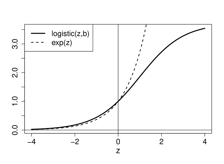
Figure 1: Logistic function $g(z)$ with $b=1$ and exponential function

Due to nonlinearity of the transformation function $g$, the field $\sigma(t,s)$ is non-Gaussian. Its pointwise distribution is known as logit-normal or logit-Gaussian.

3.2.3 $\rho(t,s)$ and $\nu(t,s)$

The remaining two secondary fields $\rho(t,s)$ and $\nu(t,s)$ (denoted here generically by $\psi$) are modeled in a way similar to $\sigma(t,s)$, the only difference being the transformation function. Specifically, the pre-transform Gaussian field $\psi^{*}$ satisfies

$$\frac{\partial\psi^{*}}{\partial t}+U_{\psi}\frac{\partial\psi^{*}}{\partial s}+\rho_{\psi}\psi^{*}-\nu_{\psi}\frac{\partial^{2}\psi^{*}}{\partial s^{2}}=\sigma_{\psi}\,\alpha_{\psi}(t,s),$$ (23)

where, again, $U_{\psi},\rho_{\psi},\nu_{\psi}$, and $\sigma_{\psi}$, are the hyperparameters and $\alpha_{\psi}$ is the independent white noise field.

The transformation function is defined here to be

$$\psi(t,s)=\overline{\psi}\cdot\left[(1+\varepsilon_{\psi})\cdot g(\psi^{*}(t,s))-\varepsilon_{\psi}\right],$$ (24)

where $\overline{\psi}$ is the unperturbed value of $\psi$, the function $g$ is the same as in section 3.2.2 and controlled by the same saturation hyperparameter $b$, and $\varepsilon_{\psi}$ is the small non-negative constant. The hyperparameter $\varepsilon_{\psi}$ is introduced to allow for small negative values of $\psi$ (that is, of $\rho$ and $\nu$). This will take place if the pre-transform Gaussian field $\psi^{*}$ happens to take a large negative value. Allowing for negative values of the decay coefficient $\rho$ and the diffusion coefficient $\nu$ is motivated by the desire to introduce an intermittent instability into the model.

Like $\sigma(t,s)$, the fields $\rho(t,s)$ and $\nu(t,s)$ are logit-Gaussian.

3.3 Third level of the hierarchy: hyperparameters and external parameters

In contrast to the popular Lorenz’96 model [28], which has only one parameter $F$, DSADM has many parameters as discussed above (in total, there are 23 hyperparameters). It is convenient to specify the hyperparameters using a set of more sensible external parameters as described next.

The advection velocities $\overline{U}$ and $U_{\theta}$ (for $\theta=U,\rho,\nu,\sigma$) are specified directly as they have a clear physical meaning.

The unperturbed hyperparameters $\overline{\theta}=\overline{\rho},\overline{\nu},\overline{\sigma}$ are specified from the unperturbed external parameters $\overline{L}$, $\overline{T}$, and $\overline{\operatorname{SD}(\xi)}$ using Eqs.(16), (14), and (12). The latter determine the desired typical spatial scale, time scale, and variance of the field $\xi(t,s)$. Note that in the non-stationary regime, $\overline{L}$, $\overline{T}$, and $\overline{\operatorname{SD}(\xi)}$ are not exactly equal to the mean values of the length scale, time scale, and variance of $\xi(t,s)$, respectively, because closed-form expressions for the latter are not available.

Likewise, for any pre-transform Gaussian field $\theta^{*}=U^{*},\rho^{*},\nu^{*},\sigma^{*}$, the respective hyperparameters $\rho_{\theta}$ and $\nu_{\theta}$ are calculated from the external parameters $L_{\theta}$ and $T_{\theta}$ using Eqs.(16) and (14). $L_{\theta}$ and $T_{\theta}$ are the user-specified spatial and temporal scales of non-stationarity.

The hyperparameters $\sigma_{\theta}$ are specified as follows. $\sigma_{U}$ is calculated from the external parameter $\operatorname{SD}(U^{*})$ using Eq.(12). For each of the other three secondary fields, $\theta=\rho,\nu,\sigma$, we select $\varkappa_{\theta}=\exp(\operatorname{SD}(\theta^{*}))$ to be the respective external parameter. This choice is motivated by the fact that these fields are nonlinearly transformed Gaussian fields. As $g(z)$ (defined in Eq.(22) and shown in Fig.1) is a “tempered” exponential function, it is worth measuring the standard deviation of, say, the $\sigma^{*}$ field on the log scale: $\operatorname{SD}(\sigma^{*})=\log\varkappa_{\sigma}$, so that the typical deviation of the transformed field $\sigma$ from its unperturbed value $\overline{\sigma}$ is $\varkappa_{\sigma}$ times. The external parameters $\operatorname{SD}(U^{*})$, $\varkappa_{\sigma}$, $\varkappa_{\rho}$, and $\varkappa_{\nu}$ determine the strength of non-stationarity.

Finally, for the fields $\psi=\rho,\nu$, we parameterize $\varepsilon_{\psi}$ (which, we recall, controls the occurrence of negative values of $\psi$) using the probability $\pi_{\psi}$ that $\psi(t,s)$ is negative:

$$P(\psi(t,s)<0)=\pi_{\psi}.$$ (25)

Substituting $\psi$ from Eq.(24) into Eq.(25) and utilizing monotonicity of the transformation function $g$ and Gaussianity of the field $\psi^{*}$, we easily come up with a relation between $\pi_{\psi}$ and $\varepsilon_{\psi}$ (the elementary formulas are omitted). The external parameters $\pi_{\rho}$ and $\pi_{\nu}$ thus determine how often and how strong local instabilities can be. (Actually, $\pi_{\psi}$ slightly impacts also $\sup\psi$, but this is a minor effect and it can be ignored in this application.)

To facilitate the use of DSADM, we introduce a reduced set of external parameters using the following constraints.

(i) The unperturbed advection velocity $\overline{U}$ and all advection velocities $U_{\theta}$ are equal to each other.

(ii) The length-scale hyperparameters $L_{\theta}$ for all pre-transform fields $\theta^{*}$ are selected to be equal to the common value $L^{*}$, the length scale of non-stationarity.

(iii) The time-scale hyperparameters $\overline{T}$ and $T_{\theta}$ are specified to be equal to $\overline{L}/V_{\rm char}$ and $L_{\theta}/V_{\rm char}=L^{*}/V_{\rm char}$, respectively, where $V_{\rm char}$ is the characteristic velocity.

(iv) The $g$-function’s saturation hyperparameter $b$ is set to 1.

Having selected a meaningful value of $V_{\rm char}$, the user can control the typical time and length scales of $\xi$, the strength of non-stationarity, and the time and length scales of non-stationarity — using the reduced set of the 10 external parameters listed in Table 1.

Table 1: Short list of external parameters of DSADM

External	Dependent	Which feature of the model is controlled?
parameter	hyperparameters
$\overline{\operatorname{SD}(\xi)}$	$\overline{\sigma}$	Mean $\operatorname{SD}(\xi)$ (roughly)
$\overline{U}$	$\overline{U},U_{U},U_{\rho},U_{\nu},U_{\sigma}$	All advection velocities
$\overline{L}$	$\overline{\rho},\overline{\nu}$	Mean length scale of $\xi$ (roughly)
$L^{*}$	$\rho_{U},\rho_{\rho},\rho_{\nu},\rho_{\sigma}$	Length scale and time scale
	$\nu_{U},\nu_{\rho},\nu_{\nu},\nu_{\sigma}$	of non-stationarity
$\operatorname{SD}(U^{*})$	$\sigma_{U}$	Strength of non-stationarity
$\varkappa_{\rho},\varkappa_{\nu},\varkappa_{\sigma}$	$\sigma_{\rho},\sigma_{\nu},\sigma_{\sigma}$	Strength of non-stationarity
$\pi_{\rho}$, $\pi_{\nu}$	$\varepsilon_{\rho}$, $\varepsilon_{\nu}$	Strength of non-stationarity
		(portions of time $\rho$ and $\nu$ are negative)

4 Properties and capabilities of DSADM

4.1 Non-stationarity

Here, we show that, given the secondary fields, the solution to DSADM is indeed a non-stationary in space and time random field. Its spatiotemporal covariances are themselves random (as they depend on the random secondary fields) and appear to be stationary processes in space-time.

Let us rewrite the basic Eq.(17) as the linear stochastic state-space model

$$\frac{d\boldsymbol{\xi}(t)}{{\rm d}t}=\boldsymbol{\Phi}(\underline{\boldsymbol{\theta}}(t))\,\boldsymbol{\xi}(t)+\boldsymbol{\Sigma}(\underline{\boldsymbol{\theta}}(t))\,\boldsymbol{\alpha}(t),$$ (26)

where $\boldsymbol{\xi}$ and $\underline{\boldsymbol{\theta}}$ stand for the vectors of the spatially gridded fields $\xi(t,s)$ and $\boldsymbol{\theta}(t,s)$, respectively, $\boldsymbol{\alpha}(t)$ is the space-discrete and time-continuous white noise, $\boldsymbol{\Phi}(\underline{\boldsymbol{\theta}})$ is the spatial operator dependent on the spatial fields $\underline{\boldsymbol{\theta}}$, and $\boldsymbol{\Sigma}(\underline{\boldsymbol{\theta}})$ is the diagonal matrix whose application to $\boldsymbol{\alpha}$ represents the forcing term $\sigma\alpha$ in Eq.(17).

Note that DSADM is intended to be used as a model-of-truth in which the secondary fields, once computed in an experiment, are held fixed. In this default setting, Eq.(26) implies that DSADM is a linear non-autonomous stochastic model (because $\boldsymbol{\Phi}$ and $\boldsymbol{\Sigma}$ are explicit functions of time).

Discretizing Eq.(26) in time (using an implicit time-differencing scheme) yields the equation for the time-discrete signal $\boldsymbol{\xi}$:

$$\boldsymbol{\xi}_{k}={\bf F}(\underline{\boldsymbol{\theta}}_{k})(\boldsymbol{\xi}_{k-1}+\boldsymbol{\Sigma}(\underline{\boldsymbol{\theta}}_{k})\boldsymbol{\alpha}_{k}),$$ (27)

where $\boldsymbol{\xi}_{k}$ is the field on the spatial grid (an $n$-vector), $k=1,2,\dots$ labels the time instant, ${\bf F}$ is the model operator, and components of the vector $\boldsymbol{\alpha}_{k}$ are independent Gaussian variables with mean zero and variance $1/(\Delta s\Delta t)$. Here $\Delta s=2\pi R/n$ is the spatial grid spacing and $\Delta t$ the time step. The initial condition $\boldsymbol{\xi}_{0}$ has mean zero and the known covariance matrix $\boldsymbol{\Gamma}_{0}$. Equation (27) allows us to find the conditional covariance matrix of the spatial field $\boldsymbol{\xi}_{k}$ given the secondary fields $\underline{\boldsymbol{\theta}}_{1:k}$ (the notation $1:k$ designates all time instants from 1 to $k$), that is, $\boldsymbol{\Gamma}_{k}=\operatorname{\mathbb{E}}(\boldsymbol{\xi}_{k}\boldsymbol{\xi}_{k}^{\top}|\underline{\boldsymbol{\theta}}_{1:k})$, using the recursion

$$\boldsymbol{\Gamma}_{k}={\bf F}(\underline{\boldsymbol{\theta}}_{k})\,\boldsymbol{\Gamma}_{k-1}\,{\bf F}(\underline{\boldsymbol{\theta}}_{k})^{\top}+{\bf Q}(\underline{\boldsymbol{\theta}}_{k}),$$ (28)

where ${\bf Q}={\bf F}\boldsymbol{\Sigma}^{2}{\bf F}^{\top}/(\Delta s\Delta t)$ is the covariance matrix of the forcing. The lagged covariances $\boldsymbol{\Gamma}_{kj}=\operatorname{\mathbb{E}}(\boldsymbol{\xi}_{k}\boldsymbol{\xi}_{j}^{\top}|\underline{\boldsymbol{\theta}}_{1:k})$ (where $j<k$) can be found by right-multiplying Eq.(27) by $\boldsymbol{\xi}_{j}^{\top}$ and taking expectation (note that for $j<k$, $\boldsymbol{\xi}_{j}$ is independent of $\boldsymbol{\alpha}_{k}$):

$$\boldsymbol{\Gamma}_{kj}={\bf F}(\underline{\boldsymbol{\theta}}_{k})\,\boldsymbol{\Gamma}_{k-1,j}.$$ (29)

Now recall that the secondary fields $\underline{\boldsymbol{\theta}}$ are random fields. Then, Eqs.(28) and (29) imply that the field (signal) covariances $\boldsymbol{\Gamma}_{k}$ and $\boldsymbol{\Gamma}_{kj}$ are (matrix variate) random processes. It can be shown that if $\rho(t,s)>0$ and $\nu(t,s)>0$ (for small enough $\pi_{\rho}$ and $\pi_{\nu}$ this is true most of the time), then ${\bf F}$ (as a matrix operator) is a contraction. Therefore, the dependence of $\boldsymbol{\Gamma}_{k}$ and $\boldsymbol{\Gamma}_{kj}$ on $\boldsymbol{\Gamma}_{0}$ fades out as $k\to\infty$ and only the secondary fields $\underline{\boldsymbol{\theta}}$ determine the covariances of $\xi(t,s)$. Moreover, since the fields $\underline{\boldsymbol{\theta}}$ are stationary in space-time and ${\bf F}$ and ${\bf Q}$ are space and time invariant (as operators acting on $\underline{\boldsymbol{\theta}}$), the field covariances $\boldsymbol{\Gamma}_{k}$ and $\boldsymbol{\Gamma}_{kj}$ are stationary random processes in space-time.

Below, we will be particularly interested in the following two aspects of the spatial covariances $\boldsymbol{\Gamma}_{k}$ or, in continuous notation and omitting for brevity the dependence on the secondary fields, $\gamma(t,t;s,s^{\prime})$: (i) the time and space specific field variance ${\mathsf{Var}}\,\xi(t,s)=\gamma(t,t;s,s)$ and (ii) a time and space specific spatial scale defined to be, say, the local macroscale:

$$\Lambda_{\xi}(t,s)=\frac{1}{2\,{\mathsf{Var}}\,\xi(t,s)}\int_{{\mathbb{S}}^{1}(R)}\gamma(t,t;s,s^{\prime}){\rm d}s^{\prime}.$$ (30)

Then, from stationarity of $\gamma(t,t;s,s^{\prime})$, it follows that both ${\mathsf{Var}}\,\xi(t,s)$ and $\Lambda_{\xi}(t,s)$ are stationary in space-time random fields.

4.2 Estimation of true covariances

Instead of the recursive computation of the field covariances using Eq.(28), one can estimate them as accurately as needed by running DSADM Eq.(17) $P$ times with independent realizations of the forcing $\alpha(t,s)$ and with the fields $\boldsymbol{\theta}(t,s)$ held fixed. The spatial covariances $\gamma(t,t;s_{1},s_{2})$ can then be estimated from the resulting sample $\{\xi^{(p)}(t,s)\}_{p=1}^{P}$ as the usual sample covariances.

More importantly, this approach can be used to estimate time and space-specific true filtering distributions of any filter in question. Note that these distributions and their parameters (e.g., true background-error covariances) are hard to obtain even knowing the model of truth. Indeed, on the one hand, a sub-optimal filter, because of its approximate nature, can only yield estimates which are inexact and, likely, biased (hence the need for covariance inflation in EnKF). On the other hand, an exact (e.g., Kalman) filter cannot be used here either — because the error statistics of the approximate filter and the exact filter differ.

To estimate, say, true background-error covariances of a filter, one may use the above fields $\{\xi^{(p)}(t,s)\}_{p=1}^{P}$ as $P$ “truths”, generate $P$ sets of “synthetic” observations (with independent errors) in space and time, and perform $P$ assimilation runs. Then, at each time, one may compute $P$ background-error vectors (by subtracting the truth $\xi^{(p)}(t,s)$ from the respective background field) and then, finally, compute their (time specific) sample covariance matrix. We experimented with DSADM on a 60-point spatial grid and found that the sample size $P=5000\mbox{--}10000$ was enough to accurately estimate true time-specific error covariances (not shown). This approach is similar to that by Bishop & Satterfield [7]; the difference is that in our approach the truth is random whilst they assume that the truth is deterministic.

4.3 Instability

The nonlinear deterministic models mentioned in the Introduction are chaotic, that is, having unstable modes (positive Lyapunov exponents), whereas DSADM is stochastic but experiencing intermittent instabilities due to the possibility for $\rho$ and $\nu$ to attain negative values. In the deterministic models instabilities are curbed by nonlinearity, whereas in DSADM, these are limited by the time the random fields $\rho$ and $\nu$ remain negative.

4.4 Gaussianity

Given $\boldsymbol{\theta}$, DSADM is linear, hence $\xi(t,s)$ is conditionally Gaussian. Unconditionally, $\xi(t,s)$ is a continuous mixture of zero-mean Gaussian distributions and so has a non-Gaussian distribution with heavy tails.

4.5 Unbeatable benchmark filter

Linearity of DSADM makes it possible to use the exact Kalman filter and thus to know how far from the optimal performance the filter in question is, which is always useful but often not possible with nonlinear deterministic models of truth.

In principle, non-stationarity combined with linearity can be achieved by taking a nonlinear model (like those mentioned in the Introduction) and using its tangent linear model. We have tried that with the Lorenz’96 model and found that even a tiny imposed model-error perturbation leads to an explosive growth of the forecast perturbation. Perhaps, some diffusion is needed to stabilize the model. This would complicate the model, but more significantly, the tangent linear model does not allow to explicitly specify the various characteristics of non-stationarity the DSADM does.

5 Behavior of the model

In this section, we numerically examine solutions to DSADM and some aspects of their spatiotemporal distributions.

5.1 Model setup

The model’s differential equations were solved numerically using an implicit upwind finite-difference scheme. The computational grid had $n=60$ points on the circle of radius $R=6370$ km. The model integration time step was $\Delta t=6$h. The external parameters of DSADM were selected to resemble the spatiotemporal structure of a mid-tropospheric meteorological field like temperature or geopotential, with one caveat: the time and length scales were chosen to be about twice as large as the respective meteorological scales (for the fields to be reasonably resolved on the 60-point spatial grid).

We specified $\overline{U}=$ 10 ms^-1, $\overline{L}=5\Delta s=3300$ km, $L^{*}=2L$ (it is meaningful to assume that the structural change in the field occurs at a larger space and time scale than the change in the random field itself), $\overline{\operatorname{SD}(\xi)}=5$ (selected arbitrarily and does not impact any conclusions), $\operatorname{SD}(U^{*})=10$ ms^-1, $b=1$, $\varkappa_{\rho}=\varkappa_{\nu}=\varkappa_{\sigma}=3$, $\pi_{\rho}=0.02$, $\pi_{\nu}=0.01$, $V_{\rm char}=3$ ms^-1 (tuned to give rise to the desired mean time scale).

5.2 $\xi(t,s)$ plots

Figure 2 compares typical spatiotemporal segments of solutions to the stationary stochastic model, Eq.(2), (panel a) and DSADM, Eq.(17), (panel b). One can see that, indeed, the non-stationary field had different structures at different areas across the domain, whilst the stationary field had the same structure everywhere. In particular, one can spot areas where the non-stationary field experienced more small-scale (large-scale) fluctuation than in the rest of the plot. These spots correspond to small (large) values of the local length scale $\Lambda_{\xi}$, see below Fig.3(b).

[][] [][]

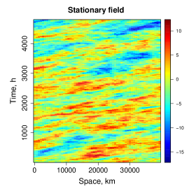
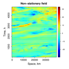
Figure 2: Realizations of $\xi(t,s)$ generated by: (a) the stationary model Eq.(2), (b) the non-stationary DSADM Eq.(17).

5.3 Non-stationarity

Figure 3 shows two characteristics of the non-stationarity pattern: the local log-variance $\log_{10}({\mathsf{Var}}\,\xi(t,s))$ and the local length scale $\Lambda_{\xi}(t,s)$ (defined in Eq.(30)). Both were calculated from the spatial covariance matrix $\boldsymbol{\Gamma}_{k}$ computed following Eq.(28). We recall that the variability in ${\mathsf{Var}}\,\xi(t,s)$ and $\Lambda_{\xi}(t,s)$ was induced by the simulated secondary fields $\boldsymbol{\theta}(t,s)$, on which ${\bf F}_{k}$ and ${\bf Q}_{k}$ depend. The same realizations of the secondary fields were used to plot both Fig.3 and Fig.2(b). In Fig.3, one can see the substantial degree of non-stationarity (note that in the stationary case both ${\mathsf{Var}}\,\xi$ and $\Lambda_{\xi}$ are constant). Specifically, in Fig.3(a), the ratio of the maximum to the minimum field variance ${\mathsf{Var}}\,\xi(t,s)$ is seen to be greater than two orders of magnitude. The same ratio for the length scale $\Lambda_{\xi}(t,s)$ (see Fig.3(b)) was about 5, which also indicates a significant degree of variation.

[][] [][]

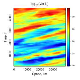
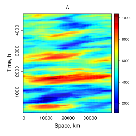
Figure 3: Space-time plots of estimated (a) field log-variance $\log_{10}({\mathsf{Var}}\,\xi(t,s))$, (b) spatial macroscale $\Lambda_{\xi}(t,s)$.

Figure 4 displays how diverse the true spatial correlations were. Note that Fig.3(a) illustrates the non-stationarity of the field’s magnitude, whereas Figs.3(b) and 4 highlight the non-stationarity of the field’s spatial structure.

Figure 4: Spatial correlations of the field $\xi$ with respect to 30 randomly selected points in space-time.

Thus, DSADM is capable of generating significantly non-stationary random fields.

5.4 Gaussianity

As noted above, conditionally on the secondary fields, $\xi(t,s)$ is Gaussian by construction. This is the way DSADM is used in this study. In principle, it can be used for other purposes without conditioning on the secondary fields, so that in each model run both the forcing and the model coefficients are random (and the model becomes autonomous). In this setting, the generated field $\xi$ is no longer Gaussian. Numerical experiments confirmed that the unconditional distribution of $\xi(t,s)$ was indeed non-Gaussian with heavy tails (as we anticipated in section 4.4). The non-Gaussianity was stronger for larger magnitudes of the secondary fields (not shown).

5.5 Forward and inverse modeling

Building DSADM can be called forward hierarchical modeling. That is, we have formulated a (hopefully) reasonable hierarchical model and an algorithm to compute realizations of the first-level random field $\xi(t,s)$ given the third-level hyperparameters $\boldsymbol{\phi}$. A harder problem is inverse modeling, that is, the inference about the model parameters—in our case the parameter fields $\boldsymbol{\theta}(t,s)$—from a number of realizations (an ensemble) of the field $\xi$. This is the classical hierarchical Bayesian problem, which is beyond the scope of this study but can be relevant in a broader context of non-stationary spatial and spatiotemporal field modeling.

6 Hybrid HBEF (HHBEF) filter

In the rest of the paper, we use DSADM to study the impact of non-stationarity on the performance of hybrid ensemble filters. We formulate a new filter that extends HBEF (in which ensemble covariances are blended with recent-past time-smoothed covariances, see Tsyrulnikov & Rakitko [43]) by introducing two additional kinds of hybridization mentioned in the Introduction: blending with climatological covariances (as in EnVar) and blending with spatially neighboring covariances (spatial smoothing). We start with a review of HBEF and then introduce HHBEF.

6.1 HBEF

Tsyrulnikov & Rakitko [43] developed, building on [33, 8, 9], their Hierarchical Bayes ensemble Kalman filter (HBEF), which cyclically updates prior covariances using ensemble members as generalized observations and the estimated previous-cycle covariances as a background. The (Bayesian) update relies on the inverse-Wishart matrix-variate hyperprior distribution for the unknown, and thus assumed random, covariance matrices.

HBEF updates the model-error and the predictability-error covariance matrices, but here we consider a simplified design in which the background-error covariance matrix ${\bf B}_{k}$ is cyclically updated. In the simplest version of HBEF, the mean-square-optimal posterior (analysis) estimate ${\bf B}^{\rm a}_{k}$ of the unknown true matrix ${\bf B}_{k}$ is the linear combination of the background ${\bf B}^{\rm f}_{k}$ and the (localized and inflated) sample covariance matrix, ${\bf B}^{\rm e}_{k}$:

$${\bf B}^{\rm a}_{k}=\frac{\vartheta{\bf B}^{\rm f}_{k}+N{\bf B}^{\rm e}_{k}}{\vartheta+N},$$ (31)

where $N$ is the ensemble size and $\vartheta>0$ the so-called sharpness parameter of the inverse Wishart distribution (defined in Appendix A in Tsyrulnikov & Rakitko [43]). The background ${\bf B}^{\rm f}_{k}$ is provided by the persistence forecast:

$${\bf B}^{\rm f}_{k}={\bf B}^{\rm a}_{k-1}.$$ (32)

The matrix ${\bf B}^{\rm a}_{k}$ computed according to Eq.(31) is used in the analysis of the state $\boldsymbol{\xi}_{k}$ as the background-error covariance matrix. The posterior (analysis) ensemble is generated in HBEF (and in all other filters in this study) in the same way as in the stochastic EnKF [e.g., 20].

From Eqs.(31) and (32), it follows that ${\bf B}^{\rm a}_{k}$ satisfies the first-order autoregressive equation

$${\bf B}^{\rm a}_{k}=\mu{\bf B}^{\rm a}_{k-1}+(1-\mu){\bf B}^{\rm e}_{k},$$ (33)

where $\mu=\vartheta/(\vartheta+N)<1$. Equation (33) implies a kind of time smoothing of ensemble covariances. In particular, ${\bf B}^{\rm a}_{k-1}$ is the time-smoothed recent-past ensemble covariance matrix denoted in what follows by ${\bf B}^{\rm r}_{k}$. With this notation, Eq.(33) shows that ${\bf B}^{\rm a}_{k}$ is a (convex) linear combination of ${\bf B}^{\rm r}_{k}$ and ${\bf B}^{\rm e}_{k}$. The role of ${\bf B}^{\rm r}_{k}$ in HBEF is two-fold. First, if spatial non-stationarity has some memory (which is highly likely in realistic systems), then ${\bf B}^{\rm r}_{k}$ brings this past memory to the current assimilation cycle, improving the accuracy of the resulting estimate of the true background-error covariance matrix ${\bf B}_{k}$. Second, due to time smoothing (i.e., averaging), the sampling noise is reduced, leading to a more accurate estimate ${\bf B}^{\rm a}_{k}$.

6.2 HHBEF: blending with static covariances

The first idea of the new hybrid-HBEF (HHBEF) filter is to replace the HBEF’s persistence forecast for the covariance matrix ${\bf B}_{k}$ (Eq.(32)) with a regression-to-the-mean forecast:

$${\bf B}^{\rm f}_{k}=w{\bf B}^{\rm a}_{k-1}+(1-w){\bf B}^{\rm c}.$$ (34)

Here, ${\bf B}^{\rm c}$ is the climatological covariance matrix and $w\in[0,1]$ is the scalar weight.

6.3 Spatial smoothing of the covariances

The second idea of HHBEF is to accommodate spatially smoothed ensemble covariances. Here, we review the approach by Buehner & Charron [11], who studied spectral-space localization, found it useful in reducing sampling noise, and noted that it is equivalent to a spatial smoothing of the covariance function — see their Eq.(9), which we rewrite here as

$$\check{B}(s_{1},s_{2})=\int_{{\mathbb{S}}^{1}(R)}\kappa(s)\,B(s_{1}-s,s_{2}-s){\rm d}s,$$ (35)

where the check $\,\check{}\,$ designates the smoothing and $\kappa(s)\geq 0$ is the weighting (averaging) function. In the space-discrete case, Eq.(35) can be approximated as follows:

$$B_{ii^{\prime}}=\sum_{s=-n/2+1}^{n/2}\kappa_{s}\,B_{i-s,i^{\prime}-s},$$ (36)

where $\kappa_{s}\geq 0$ are the weights such that $\sum\kappa_{s}=1$. In the matrix form Eq.(36) can be written as

$$\check{\bf B}=\sum_{s=-n/2+1}^{n/2}\kappa_{s}\,{\cal F}^{s}{\bf B}{\cal F}^{-s},$$ (37)

where ${\cal F}$ is the forward-shift operator. From Eq.(37) with non-negative $\kappa_{s}$ and given that ${\cal F}^{-1}={\cal F}^{\top}$, it immediately follows that the smoothing is properly defined in the sense that the resulting smoothed covariance matrix $\check{\bf B}$ is non-negatively definite.

If ${\bf B}=\frac{1}{N-1}\sum{\bf e}_{l}{\bf e}_{l}^{\top}$, where ${\bf e}_{l}$ is the $l$-th ensemble perturbation, $l=1,\dots,N$, then Eq.(37) implies that the spatial smoothing of the sample covariance matrix can be performed by spatially shifting (through the repeated application of the forward and backward shift operators) and weighting (through the multiplication by $\sqrt{\kappa_{s}}$) ensemble perturbations — as it was proposed and tested by Buehner & Charron [11].

6.4 HHBEF’s hybrid covariances

Combining Eq.(34) with Eq.(31), where ${\bf B}^{\rm e}$ is replaced by its spatially smoothed version $\check{\bf B}^{\rm e}$ computed according to Eq.(37), yields the HHBEF’s analog of the HBEF’s Eq.(33):

$${\bf B}^{\rm a}_{k}=\mu w{\bf B}^{\rm a}_{k-1}+(1-\mu)\check{\bf B}^{\rm e}_{k}+\mu(1-w){\bf B}^{\rm c},$$ (38)

where $\mu$ is the weight of ${\bf B}^{\rm f}_{k}$ relative to $\check{\bf B}^{\rm e}_{k}$. Solving Eq.(38) (which is a forced linear difference equation; the derivation is omitted) shows that, for $\mu w<1$ and after an initial transient, ${\bf B}^{\rm a}_{k}$ has the four components:

$${\bf B}^{\rm a}_{k}=w_{\rm e}{\bf B}^{\rm e}_{k}+w_{\rm es}{\bf B}^{\rm es}_{k}+w_{\rm r}{\bf B}^{\rm r}_{k}+w_{\rm c}{\bf B}^{\rm c},$$ (39)

where $w_{\rm e}=(1-\mu)\kappa_{0}$ is the weight of the current ensemble covariances ${\bf B}^{\rm e}_{k}$, $w_{\rm es}=(1-\mu)(1-\kappa_{0})$ is the weight of the spatially smoothed current ensemble covariances ${\bf B}^{\rm es}_{k}=\check{\bf B}^{\rm e}_{k}-{\bf B}^{\rm e}_{k}$, $w_{\rm c}={\mu(1-w)}/{(1-\mu w)}$ is the weight of the climatological covariances ${\bf B}^{\rm c}$, and $w_{\rm r}=\mu w(1-\mu)/(1-\mu w)$ is the weight of the spatiotemporally-smoothed recent-past ensemble covariances ${\bf B}^{\rm r}_{k}$:

$${\bf B}^{\rm r}_{k}=\frac{\check{\bf B}^{\rm e}_{k-1}+\mu w\check{\bf B}^{\rm e}_{k-2}+(\mu w)^{2}\check{\bf B}^{\rm e}_{k-3}+\dots}{1+\mu w+(\mu w)^{2}+\dots}.$$ (40)

The smoothing time scale (measured in assimilation cycles) is $-1/\log(\mu w)$.

Equations (37) and (38) show that $w=1$ and $\kappa_{s}=\delta_{s0}$ (where $\delta_{s0}$ is the Kronecker delta) reduces HHBEF to HBEF, $w=0$ to EnVar, $\mu=0$ and $\kappa_{s}=\delta_{s0}$ to pure EnKF, and $w=0,\mu=1$ recovers the filter with static background-error covariances.

Thus, HHBEF employs blending of (localized) sample covariances with both climatological and spatiotemporally-smoothed background-error covariances.

7 Performance of the three covariance-blending techniques under non-stationarity

In this section, we experimentally study how temporal smoothing of background-error covariances, their spatial smoothing, and their mixing with climatology affects the performance of the classical stochastic EnKF [e.g., 20] and HHBEF under different regimes of non-stationarity.

7.1 “Twin” experimental methodology

In the experiments below, the truth was generated using the discretized Eq.(17), that is, Eq.(27): $\boldsymbol{\xi}_{k}={\bf F}_{k}\,\boldsymbol{\xi}_{k-1}+\boldsymbol{\varepsilon}_{k}$, where $\boldsymbol{\varepsilon}_{k}$ is the time and space-discrete model forcing. The forecast operator ${\bf F}_{k}$ was available to the filters, so that, given the analysis $\boldsymbol{\xi}^{\rm a}_{k-1}$, the next-time-instant forecast was $\boldsymbol{\xi}^{\rm f}_{k}={\bf F}_{k}\boldsymbol{\xi}^{\rm a}_{k-1}$. In this setting, the model forcing $\boldsymbol{\varepsilon}_{k}$ becomes the model error (see, e.g., Tsyrulnikov & Gayfulin [42]), with its covariance matrix ${\bf Q}_{k}$ also available to the filters. We reiterate that in each experiment, the secondary fields (which determine the forecast operator and the model-error statistics), once generated, were kept fixed.

The above setting implies that non-identical true and model twins were used, with the only difference between the two models being the stochastic model error. In contrast to using different models to generate the truth and to perform the forecast, this approach provides us with the exact knowledge (and in principle, full control) of the model error statistics. It is this knowledge (along with linearity) that justifies the use of the exact Kalman filter.

7.2 Data assimilation setup

The default DSADM setup was the same as in section 5.1. The default ensemble size was $N=10$. The setup of the filters and the observation network were chosen with the intention to mimic — as much as possible with a 1D model — the setup of a realistic meteorological data assimilation scheme.

The time interval between consecutive analyses, $T_{a}$, was selected using the following criterion. The DSADM field correlation with lag $T_{a}$ should approach the typical meteorological-field correlation at lag 6h (the most widely used in operational practice assimilation cycle in global schemes). On the one hand, the mid-tropospheric 6h time correlation was estimated by Seaman [37, Fig.1(b)] using radiosonde data to be about 0.8 for the wind fields and can be interpolated to the value of about 0.95 for geopotential [34] (that is, about 0.9 on average). On the other hand, this 0.9 correlation in the DSADM field (with the default setup) occurred, on average, at the 12h lag. So, we set $T_{a}=12$h. This is twice the typical assimilation cycle in real-world systems and is consistent with the selection of $\overline{L}$ and $\overline{T}$ in section 5.1 (about twice as large as the respective typical scales of meteorological fields).

Observations were generated every assimilation cycle at every 10th spatial grid point. The observation error standard deviation (=6) was selected to ensure that the mean reduction of the forecast-error variance in the analysis was close to the value of 10% reported by Errico & Privé [15, section 8] for a realistic data assimilation system.

The weights of the spatial covariance smoothing $\kappa_{s}$ (see Eq.(37)) were specified to be a triangular function of the spatial shift $s$, so that $\kappa_{s}$ had a maximum at $s=0$ and vanished for $|s|>s_{\rm max}$. Thus, the spatial smoothing was controlled by the single parameter $s_{\rm max}$ (the length scale of the spatial smoothing measured in grid spacings).

The covariance localization was performed using the popular function by Gaspari & Cohn [16, Eq.(4.10)].

7.3 Setup of experiments

The relative roles of the three covariance-blending devices were studied by measuring, first, the performance of EnKF with each device switched on (in turn) vs. the pure EnKF, and second, by measuring the performance of HHBEF with each device switched off (again, in turn) vs. the full HHBEF. Switching on (off) the mixing with climatology is denoted by $+C$ ($-C$). Similarly, switching on (off) the spatial smoothing of background-error covariances is denoted by $+S$ ($-S$) and the temporal smoothing by $+T$ ($-T$). Technically, all filters were built within HHBEF.

Each filtering configuration was defined by the triple of the covariance-blending parameters $w$, $\mu$, and $s_{\rm max}$ as indicated in Table 2. In each experiment, the free parameters marked in the respective row of Table 2 as “Tuned” as well as the multiplicative covariance inflation and the length scale of the covariance localization were all simultaneously manually tuned to get the best performance. The tuning was sometimes tedious but the optimum was always well defined and there was no indication that it was not unique. The search for the optimum was facilitated by the observation that the better the performance of a filter, the less need for any covariance-regularization device.

Table 2: Configurations of filters

Filter	$w$	$\mu$	$s_{\rm max}$
EnKF	No effect	0	0
EnKF $+C$ (EnVar)	0	Tuned	0
EnKF $+S$	No effect	0	Tuned
EnKF $+T$ (HBEF)	1	Tuned	0
HHBEF	Tuned	Tuned	Tuned
HHBEF $-C$	1	Tuned	Tuned
HHBEF $-S$	Tuned	Tuned	0
HHBEF $-T$	0	Tuned	Tuned

The performance of a filter, ${\rm f}$, was measured by its background root-mean-square error (brmse, with respect to the known truth, in runs with 5000 assimilation cycles) relative to that of the exact Kalman filter (KF):

$${\rm rel.err}({\rm f})=\frac{{\rm brmse}({\rm f})-{\rm brmse}({\rm KF})}{{\rm brmse}({\rm KF})}.$$ (41)

The climatological background-error covariance matrix ${\bf B}^{\rm c}$ was specified in each experiment to be the time-mean KF’s background-error covariance matrix (in a run with 50,000 assimilation cycles) — for simplicity and in an attempt to reproduce the realistic situation in which only a proxy to ${\bf B}^{\rm c}$ is available.

7.4 Results

As noted in section 3.3, the non-stationarity grows with the increasing external parameters $\operatorname{SD}(U^{*})$, $\varkappa_{\rho},\varkappa_{\nu},\varkappa_{\sigma},\pi_{\rho},\pi_{\nu}$. Here we compare the filters in four regimes with different strengths of non-stationarity as detailed in Table 3.

Table 3: External parameters of DSADM in the four regimes of non-stationarity

#	Regime	$\operatorname{SD}(U^{*})$	$\varkappa_{\rho}=\varkappa_{\nu}=\varkappa_{\sigma}$	$\pi_{\rho}$	$\pi_{\nu}$
0	Stationary	0	1	0	0
1	Weakly non-stationary	5	2	0.01	0
2	Default non-stationary	10	3	0.02	0.01
3	Strongly non-stationary	20	6	0.04	0.02

Figure 5 shows the performance scores (defined in Eq.(41)) for the four configurations indicated in the upper half of Table 2 plus the full HHBEF. One can see that all three covariance-blending techniques were quite successful in improving the performance of EnKF. This could be expected because the ensemble size $N=10$ was rather small.

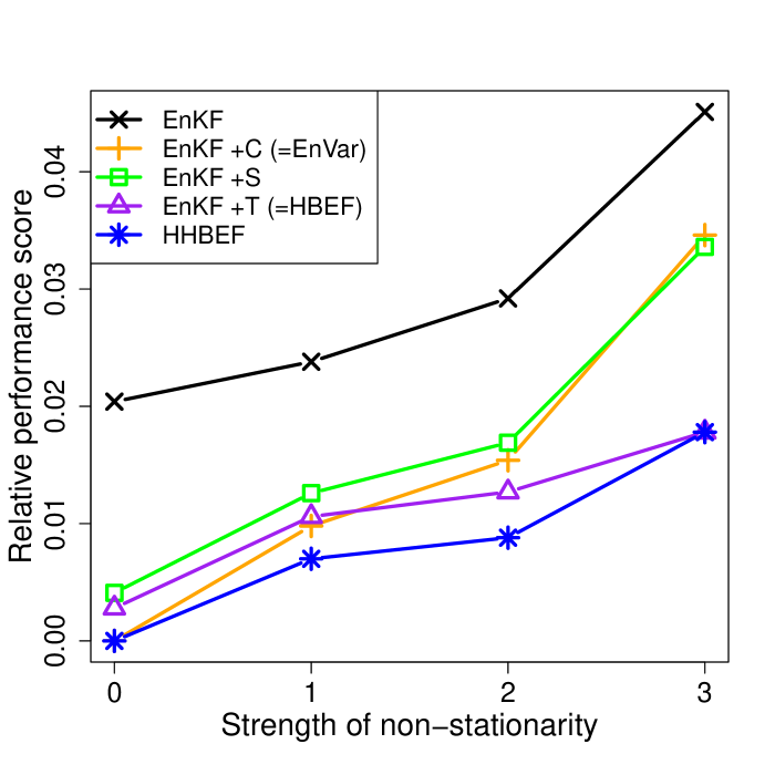
Figure 5: Performance scores (relative to KF, the lower the better) of the pure EnKF (the upper curve), EnKF with one of the three covariance-blending devices switched on (the three lower curves), and HHBEF (the lowest curve). The filters’ notation follows Table 2. The numbers on the x-axis correspond to the numbers in the first column of Table 3.

Static covariances were most useful in the low non-stationarity regimes (non-stationarity strengths 0 and 1) while being least useful under strong non-stationarity. This is reasonable because under stationarity, static covariances suffice for exact filtering, whilst they become useless when the filtering-error statistics are, typically, very different from climatology, which is the case in a highly non-stationary regime.

The temporal covariance smoothing is seen to be beneficial in all regimes, especially under strong non-stationarity, and always more efficient than the spatial covariance smoothing. The reason for the observed systematic advantage of the temporal covariance smoothing over the spatial covariance smoothing is unclear. We may conjecture that neighboring-in-space covariances bring less information because they are part of the same sample covariance matrix, whereas neighboring-in-time covariances come from a different sample covariance matrix and can therefore be more independent.

It is seen in Fig.(5) that HHBEF was more accurate than the other filters.

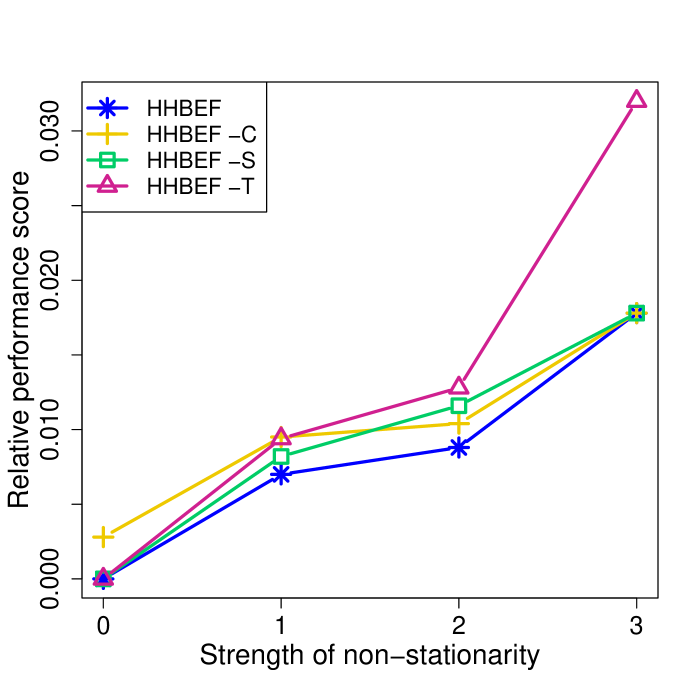
Figure 6: Same as Fig.5, but for the full HHBEF and HHBEF with one of the three covariance-blending devices switched off.

To check if the three covariance-blending techniques remained beneficial when used in combination, the four configurations indicated in the lower half of Table 2 were compared: HHBEF vs. HHBEF with one of the three covariance-blending devices withheld. Figure 6 displays the results, which were, generally, consistent with those depicted in Fig.5. Under non-stationarity, all three blending devices remained usefulr if used jointly except for the strongly non-stationary regime 3, where only time smoothing was beneficial. Not using static covariances led to the worst performance under stationarity and low non-stationarity. Switching off the time smoothing was most detrimental for the default and strong non-stationarity.

It is also of interest to inspect the optimal HHBEF’s weights: $w_{\rm e}$, $w_{\rm es}$, $w_{\rm r}$, and $w_{\rm c}$ (see Eq.(39) and the paragraph after it). The weights are plotted in Fig.7 for the same four strengths of non-stationarity as above. Overall, we see that the two dominant sources of hybrid covariances were static covariances (prevailing in the low non-stationarity regimes) and spatiotemporally-smoothed covariances (most important if the non-stationarity was high). The role of non-smoothed ensemble covariances increased with the growing non-stationarity. This is meaningful because any covariance blending reduces sampling noise but distorts the flow-dependent signal carried by the non-smoothed ensemble covariances, and this distortion grows when the covariances become more variable. The spatially averaged covariances were beneficial only for non-stationarity strengths 1 and 2 and useless under the strong non-stationarity (and of course under stationarity). This is consistent with Fig.6.

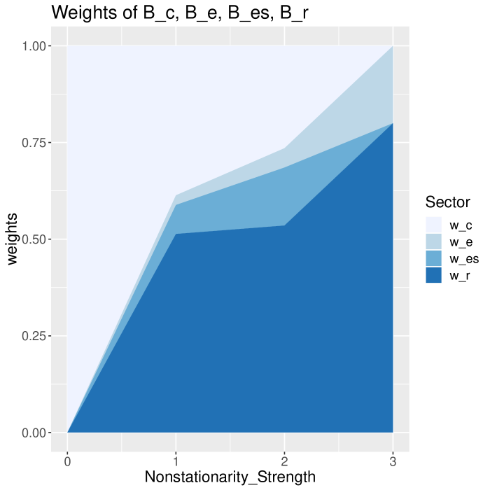
Figure 7: Optimal blending weights of climatological covariances, $w_{\rm c}$, non-smoothed current ensemble covariances, $w_{\rm e}$, spatially smoothed current ensemble covariances, $w_{\rm es}$, and spatiotemporally-smoothed recent-past covariances, $w_{\rm r}$. The numbers on the x-axis correspond to the numbers in the first column of Table 3.

We also studied how the effects of the three covariance-blending techniques depend on the time and length scales of non-stationarity (determined by the external parameter $L^{*}$, see Table 1). We found that the effects were quite stable, while blending with spatially and spatiotemporally-smoothed covariances was more beneficial for larger $L^{*}$ (not shown). This can be expected because space and time smoothing is worthwhile only if the covariances vary smoothly in space and time.

Finally, we explored the performance of the three covariance-blending techniques for large ensembles ($N=80$ and $N=300$) under the default non-stationarity. First, we found that for those ensembles, some covariance regularization was still useful. This is reasonable because for the non-regularized sample covariance matrix to be a good estimator of the true covariance matrix, the sample size must be significantly greater than the dimensionality of the matrix, see e.g., Bai & Shi [4, Section 2], that is, $N\gg n$, where, we recall, $n=60$ in our experiments. Second, the effects of all five regularization techniques (the three blending devices plus covariance localization and multiplicative covariance inflation) were significantly reduced as compared with the ensemble sizes $N=10$ (see above) and $N=30$ (not shown), which is, of course, meaningful. Third, the effect of blending with climatology was negligibly small (because two factors — variability in the covariances and large ensemble size — both reduce the usefulness of static covariances). Fourth, the effects of time and space smoothing remained positive, with time smoothing being still more useful. Fifth, only with huge ensembles ($N=3000$), EnKF needed no covariance regularization anymore (not shown).

8 Conclusions

In this paper we have presented a new doubly stochastic advection-diffusion-decay model (DSADM) on the circle. Double stochasticity means that not only the model forcing is stochastic, the model coefficients (parameters) are random as well. The parameters are specified to be transformed Gaussian random fields, with each Gaussian field satisfying its own stochastic advection-diffusion-decay model with constant coefficients. Thus, DSADM is hierarchical, built of linear stochastic partial differential equations at two levels in the hierarchy. DSADM is designed to be used as a toy model of truth to test and develop data assimilation methodologies.

The main advantage of DSADM is its capability of generating spatiotemporal random fields with tunable non-stationarity in space and time, while maintaining linearity and Gaussianity. This allows one, first, to separate effects of non-stationarity from effects of nonlinearity and non-Gaussianity (which is impossible with nonlinear models of truth). Second, linearity and Gaussianity allow the use of the Kalman filter as an unbeatable benchmark, which, again, is rarely possible with nonlinear models. With a small modification, DSADM can also be used to study the role of non-Gaussianity not caused by nonlinearity (say, non-Gaussianity of observation or model errors).

We have used DSADM to study the impact of non-stationarity on the performance of the following three covariance regularization techniques in EnKF: blending with static, time-smoothed, and space-smoothed background-error covariances. DSADM and the synthetic observation network were set up to resemble (as far as possible with a one-dimensional model) a realistic meteorological data assimilation system. We found that blending with static covariances was most beneficial in filtering regimes with low non-stationarity, while time-smoothing was most useful under medium and high non-stationarity. Space-smoothing was less efficient than time-smoothing. These findings were valid in a wide range of ensemble sizes. The role of time and space smoothing was found larger when the length and time scales of non-stationarity patterns were larger than the respective scales of the background-error field itself. A new filter termed HHBEF (Hybrid Hierarchical Bayes Ensemble Filter) that combines all three covariance-blending techniques proved to be most accurate among all configurations of the filters tested.

We believe that these results are relevant for real-world applications, but of course they are model dependent and the degree of relevance remains to be verified, especially because the model is new.

Thus, the optimal blend of ensemble covariances with climatology as well as with time-smoothed and space-smoothed background-error covariances is found to strongly depend on characteristics of non-stationarity. How large is the actual non-stationarity of the spatiotemporal background-error field in practical data assimilation systems, how large are the time and space scales of non-stationarity patterns as compared to the respective scales of the background-error field itself, how non-stationarity depends on the weather situation, season, scale, altitude, meteorological field, observation density and accuracy—all these questions remain open. Addressing these questions may help optimize hybrid filters that accommodate various covariance regularization techniques.

References

- [1]
- Apte et al. [2010] Apte, A., Auroux, D. & Ramaswamy, M. [2010], ‘Variational data assimilation for discrete Burgers equation’, Electron. J. Diff. Equ. 19, 15–30.
- Arnold [1974] Arnold, L. [1974], Stochastic differential equations, Wiley.
- Bai & Shi [2011] Bai, J. & Shi, S. [2011], ‘Estimating high dimensional covariance matrices and its applications’, Ann. Econ. Finance 12(2), 199–215.
- Banerjee et al. [2015] Banerjee, S., Carlin, B. P. & Gelfand, A. E. [2015], Hierarchical modeling and analysis for spatial data, CRC Press.
- Berre et al. [2015] Berre, L., Varella, H. & Desroziers, G. [2015], ‘Modelling of flow-dependent ensemble-based background-error correlations using a wavelet formulation in 4D-Var at Météo-France’, Quart. J. Roy. Meteor. Soc. 141(692), 2803–2812.
- Bishop & Satterfield [2013] Bishop, C. H. & Satterfield, E. A. [2013], ‘Hidden error variance theory. Part I: Exposition and analytic model’, Mon. Weather Rev. 141(5), 1454–1468.
- Bocquet [2011] Bocquet, M. [2011], ‘Ensemble Kalman filtering without the intrinsic need for inflation’, Nonlin. Process. Geophys. 18(5), 735–750.
- Bocquet et al. [2015] Bocquet, M., Raanes, P. N. & Hannart, A. [2015], ‘Expanding the validity of the ensemble Kalman filter without the intrinsic need for inflation’, Nonlinear Processes in Geophysics 22(6), 645–662.
- Bonavita et al. [2016] Bonavita, M., Hólm, E., Isaksen, L. & Fisher, M. [2016], ‘The evolution of the ECMWF hybrid data assimilation system’, Quart. J. Roy. Meteor. Soc. 142(694), 287–303.
- Buehner & Charron [2007] Buehner, M. & Charron, M. [2007], ‘Spectral and spatial localization of background-error correlations for data assimilation’, Quart. J. Roy. Meteor. Soc. 133(624), 615–630.
- Buehner et al. [2013] Buehner, M., Morneau, J. & Charette, C. [2013], ‘Four-dimensional ensemble-variational data assimilation for global deterministic weather prediction’, Nonlin. Process. Geophys. 20(5), 669–682.
- Chatfield [2016] Chatfield, C. [2016], The analysis of time series: an introduction, Chapman and Hall/CRC.
- Dunlop et al. [2018] Dunlop, M. M., Girolami, M. A., Stuart, A. M. & Teckentrup, A. L. [2018], ‘How deep are deep Gaussian processes?’, J. Machine Learn. Res. 19(1), 2100–2145.
- Errico & Privé [2014] Errico, R. M. & Privé, N. C. [2014], ‘An estimate of some analysis-error statistics using the Global Modeling and Assimilation Office observing-system simulation framework’, Quart. J. Roy. Meteor. Soc. 140(680), 1005–1012.
- Gaspari & Cohn [1999] Gaspari, G. & Cohn, S. E. [1999], ‘Construction of correlation functions in two and three dimensions’, Quart. J. Roy. Meteor. Soc. 125(554), 723–757.
- Gustafsson et al. [2014] Gustafsson, N., Bojarova, J. & Vignes, O. [2014], ‘A hybrid variational ensemble data assimilation for the HIgh Resolution Limited Area Model (HIRLAM)’, Nonlin. Process. Geophys. 21(1), 303–323.
- Hamill & Snyder [2000] Hamill, T. M. & Snyder, C. [2000], ‘A hybrid ensemble Kalman filter – 3D variational analysis scheme’, Mon. Weather Rev. 128(8), 2905–2919.
- Hansen & Smith [2001] Hansen, J. A. & Smith, L. A. [2001], ‘Probabilistic noise reduction’, Tellus A 53(5), 585–598.
- Houtekamer & Zhang [2016] Houtekamer, P. & Zhang, F. [2016], ‘Review of the ensemble Kalman filter for atmospheric data assimilation’, Mon. Wea. Rev. 144(12), 4489–4532.
- Kumar & Varaiya [2015] Kumar, P. R. & Varaiya, P. [2015], Stochastic systems: Estimation, identification, and adaptive control, Vol. 75, SIAM.
- Ledoit & Wolf [2004] Ledoit, O. & Wolf, M. [2004], ‘A well-conditioned estimator for large-dimensional covariance matrices’, J. Multivar. Anal. 88(2), 365–411.
- Lindgren et al. [2011] Lindgren, F., Rue, H. & Lindström, J. [2011], ‘An explicit link between Gaussian fields and Gaussian Markov random fields: the stochastic partial differential equation approach’, J. Roy. Statist. Soc. B 73(4), 423–498.
- Lorenc [2003] Lorenc, A. C. [2003], ‘The potential of the ensemble Kalman filter for NWP — a comparison with 4D-Var’, Quart. J. Roy. Meteor. Soc. 129(595), 3183–3203.
- Lorenc [2017] Lorenc, A. C. [2017], ‘Improving ensemble covariances in hybrid variational data assimilation without increasing ensemble size’, Quart. J. Roy. Meteor. Soc. 143(703), 1062–1072.
- Lorenz [1963] Lorenz, E. [1963], ‘Deterministic nonperiodic flow’, J. Atmos. Sci. 20(2), 130–141.
- Lorenz [2005] Lorenz, E. [2005], ‘Designing chaotic models’, J. Atmos. Sci. 62(5), 1574–1587.
- Lorenz & Emanuel [1998] Lorenz, E. N. & Emanuel, K. A. [1998], ‘Optimal sites for supplementary weather observations: Simulation with a small model’, J. Atmos. Sci. 55(3), 399–414.
- Ménétrier & Auligné [2015] Ménétrier, B. & Auligné, T. [2015], ‘Optimized localization and hybridization to filter ensemble-based covariances’, Mon. Weather Rev. 143(10), 3931–3947.
- Ménétrier et al. [2015] Ménétrier, B., Montmerle, T., Michel, Y. & Berre, L. [2015], ‘Linear filtering of sample covariances for ensemble-based data assimilation. Part I: Optimality criteria and application to variance filtering and covariance localization’, Mon. Weather Rev. 143(5), 1622–1643.
- Miller et al. [1994] Miller, R. N., Ghil, M. & Gauthiez, F. [1994], ‘Advanced data assimilation in strongly nonlinear dynamical systems’, J. Atmos. Sci. 51(8), 1037–1056.
- Muccino & Bennett [2002] Muccino, J. & Bennett, A. [2002], ‘Generalized inversion of the Korteweg–de Vries equation’, Dyn. Atmos. Oceans 35(3), 227–263.
- Myrseth & Omre [2010] Myrseth, I. & Omre, H. [2010], ‘Hierarchical ensemble Kalman filter’, SPE Journal 15(2), 569–580.
- Olevskaya [1968] Olevskaya, S. M. [1968], ‘The use of the canonical-correlation method in analyzing the geopotential field’, Izv. Atmos. Ocean. Phys. 4, 1149–1159.
- Piterbarg & Ostrovskii [2013] Piterbarg, L. & Ostrovskii, A. [2013], Advection and diffusion in random media: implications for sea surface temperature anomalies, Springer Science & Business Media.
- Roininen et al. [2016] Roininen, L., Girolami, M., Lasanen, S. & Markkanen, M. [2016], ‘Hyperpriors for Matérn fields with applications in Bayesian inversion’, arXiv preprint arXiv:1612.02989 .
- Seaman [1975] Seaman, R. [1975], ‘Distance-time autocorrelation functions for winds in the Australian region’, Austral. Meteorol. Mag. 23(2), 27–40.
- Sigrist et al. [2015] Sigrist, F., Künsch, H. R. & Stahel, W. A. [2015], ‘Stochastic partial differential equation based modelling of large space-time data sets’, J. Roy. Statist. Soc. B 77(1), 3–33.
- Tjøstheim [1986] Tjøstheim, D. [1986], ‘Some doubly stochastic time series models’, J. Time Ser. Anal. 7(1), 51–72.
- Tsyroulnikov [2001] Tsyroulnikov, M. D. [2001], ‘Proportionality of scales: An isotropy-like property of geophysical fields’, Quart. J. Roy. Meteor. Soc. 127(578), 2741–2760.
- Tsyrulnikov & Gayfulin [2016] Tsyrulnikov, M. & Gayfulin, D. [2016], ‘A spatio-temporal stochastic pattern generator for simulation of uncertainties in geophysical ensemble prediction and ensemble data assimilation’, arXiv:1605.02018 .
- Tsyrulnikov & Gayfulin [2017] Tsyrulnikov, M. & Gayfulin, D. [2017], ‘A limited-area spatio-temporal stochastic pattern generator for simulation of uncertainties in ensemble applications’, Meteorol. Zeitschrift 26(5), 549–566.
- Tsyrulnikov & Rakitko [2017] Tsyrulnikov, M. & Rakitko, A. [2017], ‘A hierarchical Bayes ensemble Kalman filter’, Physica D 338, 1–16.
- Whittle [1986] Whittle, P. [1986], Systems in stochastic equilibrium, John Wiley & Sons, Inc.
- Wikle et al. [1998] Wikle, C. K., Berliner, L. M. & Cressie, N. [1998], ‘Hierarchical Bayesian space-time models’, Environ. Ecol. Stat. 5(2), 117–154.
- Yaglom [1987] Yaglom, A. M. [1987], Correlation theory of stationary and related random functions, Volume 1: Basic results, Springer Verlag.