Deterministic Digital Clustering of Wireless Ad Hoc Networks

Abstract

We consider deterministic distributed communication in wireless ad hoc networks of identical weak devices under the SINR model without predefined infrastructure. Most algorithmic results in this model rely on various additional features or capabilities, e.g., randomization, access to geographic coordinates, power control, carrier sensing with various precision of measurements, and/or interference cancellation. We study a pure scenario, when no such properties are available.

The key difficulty in the considered pure scenario stems from the fact that it is not possible to distinguish successful delivery of message sent by close neighbors from those sent by nodes located on transmission boundaries. This problem has been avoided by appropriate model assumptions in many results, which simplified algorithmic solutions.

As a general tool, we develop a deterministic distributed clustering algorithm, which splits nodes of a multi-hop network into clusters such that: (i) each cluster is included in a ball of constant diameter; (ii) each ball of diameter $1$ contains nodes from $O(1)$ clusters. Our solution relies on a new type of combinatorial structures (selectors), which might be of independent interest.

Using the clustering, we develop a deterministic distributed local broadcast algorithm accomplishing this task in $O(\Delta\log^{*}N\log N)$ rounds, where $\Delta$ is the density of the network. To the best of our knowledge, this is the first solution in pure scenario which is only $\text{polylog}(n)$ away from the universal lower bound $\Omega(\Delta)$, valid also for scenarios with randomization and other features. Therefore, none of these features substantially helps in performing the local broadcast task.

Using clustering, we also build a deterministic global broadcast algorithm that terminates within $O(D(\Delta+\log^{*}N)\log N)$ rounds, where $D$ is the diameter of the network. This result is complemented by a lower bound $\Omega(D\Delta^{1-1/\alpha})$, where $\alpha>2$ is the path-loss parameter of the environment. This lower bound, in view of previous work, shows that randomization or knowledge of own location substantially help (by a factor polynomial in $\Delta$) in the global broadcast. Therefore, unlike in the case of local broadcast, some additional model features may help in global broadcast.

Corresp. author: T. Jurdzinski, (tju@cs.uni.wroc.pl) Regular paper, eligible for the best student paper award – M. Różański is a full time PhD student and has made a significant contribution.

1 Introduction

We study distributed algorithms in ad hoc wireless networks in the SINR (Signal-to-Interference-and-Noise Ratio) model with uniform transmission power. We consider the ad hoc setting where both capability and knowledge of nodes are limited – nodes know only the basic parameters of the SINR model (i.e., $\alpha,\beta,\varepsilon,\mathcal{N}$) and upper bounds $\Delta$, $n$ on the degree and the size of the network, such that the actual maximal degree is $O(\Delta)$ and the size is $n^{O(1)}$. Such a setting appears in networks without infrastructure of base nodes, access points, etc., reflecting e.g. scenarios where large sets of sensors are distributed in an area of rescue operation, environment monitoring, or in prospective internet of things applications. Among others, we study basic communication problems as global and local broadcast, as well as primitives used as tools to coordinate computation and communication in the networks (e.g., leader election and wake-up). Most of these problems were studied in the model of graph-based radio networks over the years. Algorithmic study of the closer to reality SINR model has started much later. This might be caused by specific dynamics of interferences and signal attenuation, which seems to be more difficult for modeling and analysis than graph properties appearing in the radio network model (see e.g. [28]).

As for the problems studied in this paper, several distributed algorithms have been presented in recent years. However, all these solutions were either randomized or relied on the assumption that nodes of a network know their own coordinates in a given metric space. In contrast, the aim of this paper is to check how efficient could be solutions without randomization, availability of locations, power control, carrier sensing, interference cancellation or other additional model features, in the context of local and global communication problems. Our research objective is motivated twofolds. Firstly, examination of necessity of randomization is a natural research topic in algorithmic community for classic models of sequential computation as well as for models of parallel and distributed computing (see e.g. [3] for an example in a related radio networks model). Moreover, as wireless ad hoc networks are usually built from computationally limited devices run on batteries, it is desirable to use simple and energy efficient algorithms which do not need access to several sensing capabilities or true randomness.

1.1 The Network Model.

We consider a wireless network consisting of nodes located on the 2-dimensional Euclidean space. We model transmissions in the network with the SINR constraints. The model is determined by fixed parameters: path loss $\alpha>2$, threshold $\beta>1$, ambient noise $\mathcal{N}>0$ and transmission power $\mathcal{P}$. The value of $SINR(v,u,{\mathcal{T}})$ for given nodes $u,v$ and a set of concurrently transmitting nodes ${\mathcal{T}}$ is defined as

$$SINR(v,u,{\mathcal{T}})=\frac{\mathcal{P}/d(v,u)^{\alpha}}{{\mathcal{N}}+\sum_{w\in{\mathcal{T}}\setminus\{v\}}\mathcal{P}/d(w,u)^{\alpha}},$$ (1)

where $d(u,v)$ denotes the distance between $u$ and $v$. A node $u$ successfully receives a message from $v$ iff $v\in{\mathcal{T}}$ and $SINR(v,u,{\mathcal{T}})\geq\beta$, where ${\mathcal{T}}$ is the set of nodes transmitting at the same time. Transmission range is the maximal distance at which a node can be heard provided there are no other transmitters in the network. Without loss of generality we assume that the transmission range is all equal to $1$. This assumption implies that the relationship $\mathcal{P}=\mathcal{N}\beta$ holds. However, it does not affect generality and asymptotic complexity of presented results.

Communication graph In order to describe the topology of a network as a graph, we set a connectivity parameter $\varepsilon\in(0,1)$. The communication graph $G=(V,E)$ of a given network consists of all nodes and edges $\{v,u\}$ connecting nodes that are in distance at most $1-\varepsilon$, i.e., $d(u,v)\leq 1-\varepsilon$. Observe that a node can receive a message from a node that is not its neighbor in the graph, provided interference from other nodes is small enough. The communication graph, defined as above, is a standard notion in the analysis of ad hoc multi-hop communication in the SINR model, cf., [10, 25].

Synchronization and content of messages We assume that algorithms work synchronously in rounds. In a single round, a node can transmit or receive a message from some node in the network and perform local computation. The size of a single message is limited to $O(\log N)$.

Knowledge of nodes Each node has a unique identifier from the set $[N]=\{1,\ldots,N\}$, where $N=n^{O(1)}$ is the upper bound on the size $n$ of the network. Moreover, nodes know $N$, the SINR parameters – $\mathcal{P},\alpha,\beta,\varepsilon,\mathcal{N}$, the linear upper bounds on the diameter $D$ and the degree $\Delta$ of the communication graph.

Communication problems The global broadcast problem is to deliver a message from the designated source node $s$ to all the nodes in the network, perhaps through relay nodes as not all nodes are within transmission range of the source in multi-hop networks. At the beginning of an execution of a global broadcast algorithm, only the source node $s$ is active (i.e., only $s$ can participate in the algorithm’s execution). A node $v\neq s$ starts participating in an execution of the algorithm only after receiving the first message from another node. (This is so-called non-spontaneous wake-up model, popular in the literature.) In the local broadcast problem, the goal is to make each node to successfully transmit its own message to its neighbors in the communication graph. Here, all nodes start participating in an algorithm’s execution at the same round.

1.2 Related Work

In the last years the SINR model was extensively studied, both from the perspective of its structural properties [2, 20, 28] and algorithm design [16, 4, 10, 18, 22, 35, 29, 21].

The first work on local broadcast in SINR model by Goussevskaia et al. [16] presented an $O(\Delta\log n)$ randomized algorithm under assumption that density $\Delta$ is known to nodes. After that, the problem was studied in various settings. Halldorsson and Mitra presented an $O(\Delta+\log^{2}n)$ algorithm in a model with feedback [19]. Recently, for the same setting Barenboim and Peleg presented solution working in time $O(\Delta+\log n\log\log n)$ [4]. For the scenario when the degree $\Delta$ is not known Yu et al. in [35] improved on the $O(\Delta\log^{3}n)$ solution of Goussevskaia et al. to $O(\Delta\log n+\log^{2}n)$.

In [22] a $O(\Delta\log^{3}n)$-round deterministic local broadcast algorithm was presented under the assumption that nodes have access to location information (their coordinates). However, no deterministic algorithm for local broadcast was known in the scenario that nodes do not know their coordinates.

Previous results on local broadcast are collected and compared with our result in Table 1. There are also a few algorithms which require carrier sensing or power control (e.g., [15]). As the model and techniques in this line of work are far from the topic of our paper, those solutions are not presented in the table.

Paper	Model	Knowledge	Time
Randomized algorithms
[16]		$\Delta,n$	$O(\Delta\log n)$
[16]		$n$	$O(\Delta\log^{3}n)$
[35]		$n$	$O(\Delta\log n+\log^{2}n)$
[19]	feedback	$\Delta,n$	$O(\Delta+\log^{2}n)$
[4]	feedback	$\Delta,n$	$O(\Delta+\log n\log\log n)$
Deterministic algorithms (for $N=\text{poly}(n)$)
[22]	location	$\Delta,N$	$O(\Delta\log^{3}n)$
This work		$\Delta,N$	$O(\Delta\log^{*}n\log n)$

Table 1: Algorithms for the local broadcast problem. The column Model enumerates features which do not appear in the model of this paper, while they are needed to implement particular algorithms.

For the global broadcast problem a few deterministic solutions are known. If the information about location of nodes is available, the global broadcast can be accomplished deterministically in time $O(D\log^{2}n)$ [26]. In contrast, if connectivity of a network might rely on so-called weak links and the model does not allow for any channel sensing nor access to geographic coordinates, deterministic global broadcast requires $\Theta(n\log N)$ rounds [27], which gives logarithmic improvement over $O(n\log^{2}n)$-time algorithm from [10] for this model.

The main randomized results on global broadcast in ad hoc settings include papers of Daum et al. [10] and Jurdzinski et al. [25]. Solutions with complexity, respectively $O((D\log n)\log^{\alpha+1}g)$ and $O(D\log^{2}n)$ are presented, where $g$ is a parameter depending on the geometry of the network, at most exponential with respect to $n$. (Results on global broadcast are collected and compared with our result in Table 2.)

Recently Halldorsson et al. [18] proposed an algorithm which can be faster assuming that nodes are equipped with some extra capabilities (e.g., detection whether a received message is sent from a close neighbor) and the interference function on the local (one-hop) level is defined as in the classic radio network model. Given additional model features as channel/carrier sensing, total interference estimation by signal measurements and others, efficient algorithms for various communication problems have been designed in recent years, e.g., [17, 33, 31].

Paper	Model:	Model:	Knowledge	Time
	extra features	weaknesses
Randomized algorithms
[10]			$n$	$O((D\log n)\log^{\alpha+1}g)$
[10]		weak links	$n$	$O(n\log^{2}n)$
[24]	location		$n$	$O(D\log n+\log^{2}n)$
[25]			$n$	$O(D\log^{2}n)$
Deterministic algorithms (for $N=\text{poly}(n)$)
[26]	location		$N$	$O(D\log^{2}n)$
[27]		weak links	$N$	$\Theta(n\log n)$
This work			$\Delta,N$	$\Omega(D\Delta^{1-1/\alpha})$
This work			$\Delta,N$	$O(D(\Delta+\log^{*}n)\log n)$

Table 2: Algorithms for the global broadcast problem.

In the related multi-hop radio network model the global broadcast problem is well examined. The complexity of randomized broadcast is of order of $\Theta((D+\log n)\log(n/D))$ [3, 9, 30]. A series of papers on deterministic global broadcast give the upper bound of $O(n\min\{\log n,\log D\log\log(D\Delta/n)\}$ [5, 9, 11] with the lower bound of $\Omega(n\log D)$ [6] and $\Omega(n\log n/\log(n/D))$ [30]. In terms of $\Delta$ and $D$, the best bounds are $O(D\Delta\log(N/\Delta)\log^{1+\alpha}N)$ and $\Omega(D\Delta\log(N/\Delta)$ [7]. For the closest to our model geometric unit-disk-graph radio networks, the complexity of broadcast is $\Theta(D\Delta)$ [12, 13], even when nodes know their coordinates.

Recently, communication algorithms have been also designed in a very weak beeping networks [8, 14], where a node can only distinguish between $0$ or at least one of its neighbors transmitting on the communication channel.

1.3 Our Contribution

As a general tool, we develop a clustering algorithm which splits nodes of a multi-hop network into clusters such that: (i) each cluster is included in a ball of constant diameter; (ii) each ball of diameter $1$ contains nodes from $O(1)$ clusters. Using the clustering algorithm, we develop a local broadcast algorithm for ad hoc wireless networks, which accomplishes the task in $O((\Delta+\log^{*}n)\log n)$ rounds, where $\Delta$ is the density of the network. Up to our knowledge, this is the first solution in the considered pure ad hoc scenario which is only $\text{polylog}(n)$ away from the trivial universal lower bound $\Omega(\Delta)$, valid also for scenarios with randomization and other features.

Using clustering, we also build a deterministic global broadcasting algorithm that terminates within $O(D(\Delta+\log^{*}n)\log n)$ rounds, where $D$ is the diameter of the network graph. This result is complemented by a lower bound $\Omega(D\Delta^{1-1/\alpha})$ in the network of degree $\Delta$, where $\alpha>2$ is the path-loss parameter of the environment. This lower bound, in view of previous work, shows that randomization or knowledge of own location substantially help (by a factor polynomial in $\Delta$) in the global broadcast. Previous results on global broadcast in related models achieved time $O(D\,\text{polylog}N)$, thus they were independent of the networks density $\Delta$. They relied, however, on either randomization, or access to coordinates of nodes in the Euclidean space, or carrier sensing (a form of measurement of strength of received signal). Without these capabilities, as we show, the polynomial dependence of $\Delta$ is unavoidable.

Therefore, our results prove that additional model features may help in global communication problems, but not much in local problems such as local broadcast, in which advanced algorithms are (almost) equivalent to the presence of additional model features. Using designed algorithmic techniques we also provide efficient solutions to the wake-up problem and the global leader election problem.

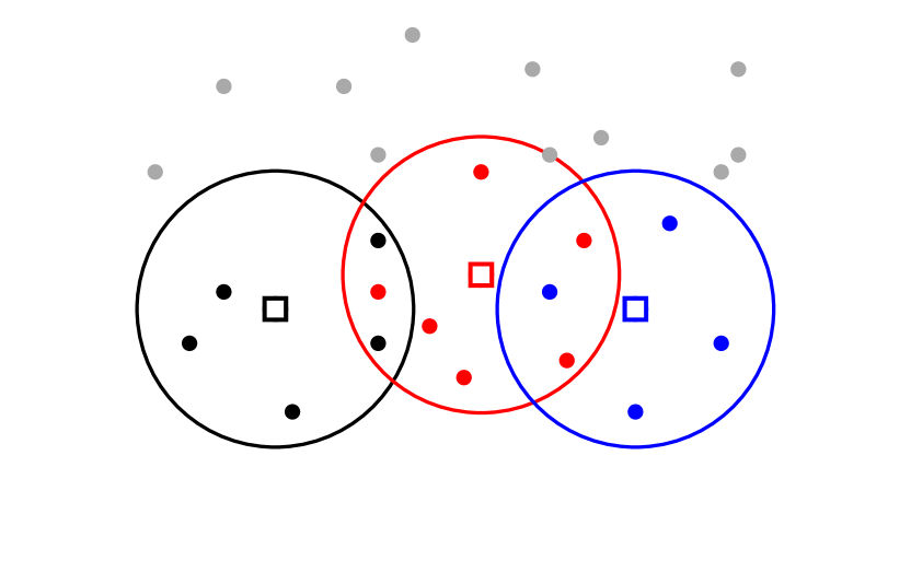
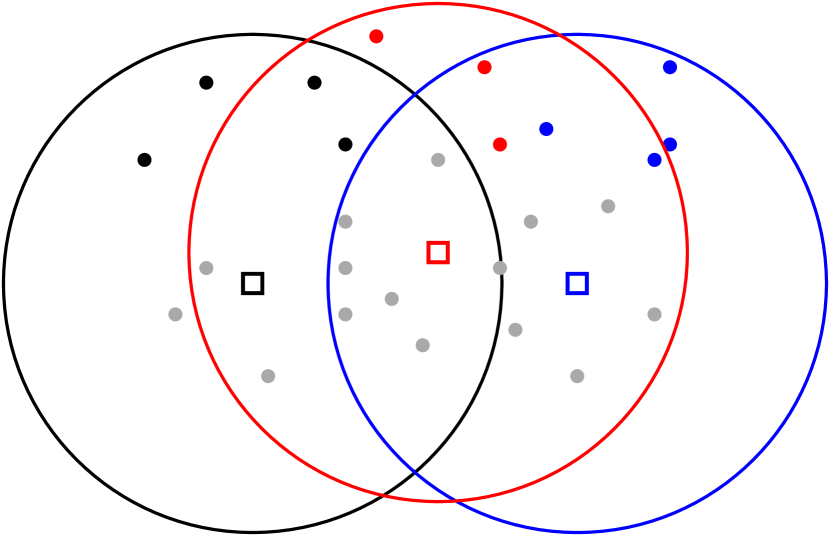
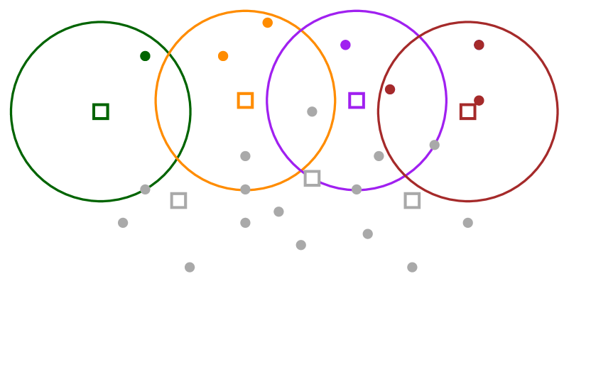
tabular 1.4 High Level Description of Our Technique The key challenge in designing efficient algorithm in the ad hoc wireless scenario is the interference from dense areas of a network. Note that if randomization was available, nodes could adjust their transmission probabilities and/or signal strength such that the expected interference from each ball of radius $1$ is bounded by a constant. Another problem stems from the fact that it is impossible to distinguish received messages which are sent by close neighbors from those sent by nodes on boundaries of the transmission range. This issue could be managed if nodes had access to their geographic coordinates or were equipped with carrier sensing capabilities (thanks to them, the distance of a neighbor can be estimated based on a measurement of the strength of received signal). In the pure ad hoc model considered in this paper, all those tools are not available. Our algorithmic solutions rely on the notion of $r$-clustering, i.e., a partition of a set of nodes into clusters such that: (i) each cluster is included in a ball of radius $r$; (ii) each ball of radius $1$ contains nodes from $O(1)$ clusters and (iii) each node knows its cluster ID. First, we develop tools for (partially) clustered networks. We start with a sparsification algorithm, which, given a set of clustered nodes $W$, gradually decreases the largest number of nodes in a cluster and eventually ends with a set $W^{\prime}\subset W$ such that $O(1)$ (and at least one!) nodes from each cluster of $W$ belongs to $W^{\prime}$. Using sparsification algorithm, we develop a tool for imperfect labeling of clusters, which results in assigning temporary IDs (tempID) in range $O(\Delta)$ to nodes such that $O(1)$ nodes in each cluster have the same tempID. Moreover, an efficient radius reduction algorithm is presented, which transforms $r$-clustering for $r>1$ into $1$-clustering. Two communication primitives are essential for efficient implementation of our tools, namely, Sparse Network Schedule (SNS) and Close Neighbors Schedule (CNS). Sparse Network Schedule is a communication protocol of length $O(\log N)$ which guarantees that, given an arbitrary set of nodes $X$ with constant density, each element $v$ of $X$ performs local broadcast (i.e., there is a round in which the message transmitted by $v$ is received in distance $1-\varepsilon$). Close Neighbors Schedule is a communication protocol of length $O(\log N)$ which guarantees that, given an arbitrary set of nodes $X$ of density $\Gamma$ with $r$-clustering of $X$ for $r=O(1)$, each close enough pair of elements of $X$ from each sufficiently dense cluster can hear each other during the schedule. Given the above described tools for clustered set of nodes, we build a global broadcasting algorithm, which works in phases. In the $i$th phase we assure that all nodes awaken in the $(i-1)$-st phase perform local broadcast. In this way, the set of nodes awaken in the first $i$ phases contains all nodes in communication graph of distance $i$ from the source. Moreover, we assure that all nodes awaken in a phase are $1$-clustered. (We start with the cluster formed by nodes in distance $\leq 1$ from the source $s$, awaken in a round in which $s$ is the unique transmitter.) A phase consists of three stages. In Stage 1, an imperfect labeling of each cluster is done. In Stage 2, Sparse Network Schedule is executed $\Delta$ times. A node with label $j$ participates in the $j$th execution of SNS only. In this way, all nodes transmit successfully on distance $1-\varepsilon$. All nodes awaken in Stage 2 inherit cluster ID from nodes which awaken them. In this way, we have $2$-clustering of all nodes awaken in Stage 2. In Stage 3, a $1$-clustering of awaken nodes is formed by using an efficient algorithm that reduces the radius of clustering. Figure 1 provides an example describing a phase. (a) Black, red and blue nodes were awaken in phase $i-1$, they are $1$-clustered (colors correspond to clusters). Gray nodes are asleep neighbors of awaken nodes. (b) In Stage 2, asleep nodes (gray in Figure (a); black, red and blue in Figure (b)) receive messages from their awaken neighbors. After Stage 2 of phase $i$, newly awaken nodes inherit cluster IDs (colors) of neighbors which awaken them. (c) In Stage 3, newly awaken nodes build a new $1$-clustering, using the algorithm which “reduces” a $2$-clustering to a $1$-clustering. Figure 1: An illustration of phase $i>1$ of the global broadcast algorithm. Squares denote centres of clusters (corresponding to nodes from these clusters). (a) Black, red and blue nodes were awaken in phase $i-1$, they are $1$-clustered (colors correspond to clusters). Gray nodes are asleep neighbors of awaken nodes.

Table 3: Local broadcast algorithms

2 Preliminaries

Geometric definitions Let $B(x,r)$ denote the ball of radius $r$ around point $x$ on the plane. That is, $B(x,r)=\{y\,|\,d(x,y)\leq r\}$. We identify $B(x,r)$ with the set of nodes of the network that are located inside $B(x,r)$. A unit ball is a ball with radius $1$. Let $\chi(r_{1},r_{2})$ denote the maximal size of a set of points $S$ located in a ball of radius $r_{1}$ such that $d(u,v)\geq r_{2}$ for each $u,v\in S$ such that $u\neq v$.

Clustered and unclustered sets of nodes Assume that each node from a given set is associated with a pair of numbers $(v,\phi)$, where $v\in[N]$ is its unique ID and $\phi\in[N]$ is the cluster of $v$, $\phi=\text{cluster}(v)$. A set $X$ of pairs $(v,\phi)$ associated to nodes is called a clustered set of nodes. The set $X$ is partitioned into clusters, where cluster $\phi$ denotes the set $\{(v,\phi^{\prime})\in X\,|\,\phi^{\prime}=\phi\}$.

An unclustered set $X$ of nodes is just a subset of $[N]$, which might be also considered as a clustered set, where each node’s cluster ID is equal to $1$, i.e., $\text{cluster}(v)=1$ for each $v\in X$.

Geometric clusters Consider a clustered set of nodes $X$ such that each node is located in the Euclidean plane (i.e, it has assigned coordinates determining its location). The clustering of $X$ is an $r$-clustering for $r\geq 1$ if the following conditions are satisfied:

• For each cluster $\phi$, all of nodes from the cluster $\phi$ are located in the ball $B(x,r)$, where $x$ is an element of $\phi$ called the center of $\phi$.

• For each clusters $\phi_{1},\phi_{2}$, the centers $x_{1},x_{2}$ of $\phi_{1},\phi_{2}$ are located in distance at least $1-\varepsilon$, i.e., $d(x_{1},x_{2})\geq 1-\varepsilon$.

The density $\Gamma$ of an unclustered network/set denotes the largest number of nodes in a unit ball. For a clustered network/set $G$, the density is equal to the largest number of elements of a cluster. Below, we characterize dependencies between the degree of the communication graph and the density of the network.

Fact 1:

Let $\Delta_{V}$ be equal to the largest degree in the communication graph $G$. Then,

1. There exist constants $0<c_{1}<c_{2}$ such that the density of each unclustered network $V$ is in the range $[c_{1}\Delta_{V},c_{2}\Delta_{V}]$.

2. There exist constants $0<c_{1}<c_{2}$ such that the density of each $r$-clustered network $V$ for $r\in[1,2]$ is in the range $[c_{1}\Delta_{V},c_{2}\Delta_{V}]$.

As the density of a network and the degree of its communication graph are linearly dependent, we will use $\Delta$/$\Gamma$ to denote both the density and the degree of the communication graph. For a clustered set of density $\Gamma$, a cluster is dense when it contains at least $\Gamma/2$ elements. Similarly, for an unclustered set of density $\Gamma$, a unit ball ${\mathcal{B}}$ is dense when it contains at least $\Gamma/2$ elements.

In the following, we define the notion of a close pair, essential for our network sparsification technique. Let $d_{\Gamma,r}$ be the smallest number satisfying the inequality $\chi(r,d_{\Gamma,r})\geq\Gamma/2$. Thus, according to the definition of the function $\chi$ and the definition of a dense cluster/ball, the smallest distance between nodes of a dense cluster (unit ball, resp.) in an $r$-clustered (unclustered, resp.) network is at most $d_{\Gamma,r}$ ($d_{\Gamma,1}$, resp.).

Definition 1:

Nodes $u,w$ form a close pair in an $r$-clustered network of density $\Gamma$ if the following conditions hold for some $\zeta\in(0,1]$ and cluster $\phi$:

1. $\text{cluster}(u)=\text{cluster}(w)=\phi$,

2. $d(u,w)=\zeta d_{\Gamma,r}\leq 1-\varepsilon$,

3. $d(u,x)\geq d(u,w)$ and $d(w,x)\geq d(u,w)$ for each $x\not\in\{u,w\}$ from the cluster $\phi=\text{cluster}(u)=\text{cluster}(w)$;

4. $d(u^{\prime},w^{\prime})\geq d(u,w)/2$ for any $u^{\prime}\neq w^{\prime}$ such that $u^{\prime},w^{\prime}\in B(u,\zeta)\cup B(w,\zeta)$ and $\text{cluster}(u^{\prime})=\text{cluster}(w^{\prime})=\phi$.

The nodes $u,w$ form a close pair in an unclustered network of density $\Gamma$ iff the above conditions (a)–(d) hold provided $\text{cluster}(x)=1$ for each node $x$ of a network and $r=1$.

A node $v$ is a close neighbor of a node $u$ iff $(u,v)$ is a close pair.

An intuition behind the requirements of the definition of a close pair is as follows. In the clustered case, only the pairs inside the same cluster are considered to be a close pair, by (a). The requirement of (b) states that $u$ and $w$ can form a close pair only in the case that $d(u,w)$ is at most the upper bound on the smallest distance between closest nodes of a dense cluster/ball. The item (c) assures that $u$ is the closest node to $w$ and $w$ is the closest node $u$. Finally, (d) states that $u$ and $w$ can be a close pair only in the case that the distances between nodes in their close neighbourhood are not much smaller than $d(u,w)$. This requirement’s goal is to count $u,w$ as a close pair only in the case that $d(u,w)$ is of the order of the smallest distance between nodes in some neighbourhood. Polynomial attenuation of strength of signals with the power $\alpha>2$ in the SINR model will assure that, for a close pair $u,w$, a successful reception of a message from $u$ to $w$ will depend on behaviour of some constant number of the nodes which are closest to $u$ and $w$. We formalize this intuition in further part of this work (Lemmas 5 and 6). In the following lemma we observe presence of close pairs in dense areas of a network.

Lemma 1:

Assume that the density of a set of nodes $X$ is $\Gamma$. Then,

1. If $X$ is unclustered, then there is a close pair in each ball $B(x,5)$ such that $B(x,1)$ is dense.

2. If $X$ is clustered, then there is a close pair in each dense cluster.

Imperfect labeling Assume that a clustering of a set $X$ of nodes with density $\Gamma$ is given. Then, $c$-imperfect labeling of $X$ is a labeling of all elements of $X$ such that label$(x)\leq\Gamma$ for each $x\in X$ and, for each cluster $\phi\in[N]$ and each label $l\in[N]$, the number of nodes from the cluster $\phi$ with label $l$ is at most $c$, where $c$ is a fixed constant. That is, the labeling is “imperfect” in the sense that, instead of unique labels, we guarantee that each label is assigned to at most $c$ nodes in a cluster.

3 Combinatorial Tools for SINR communication

In this section, we introduce combinatorial structures applied in our algorithms and basic communication primitives using these structures.

3.1 Combinatorial tools

In this section we will apply the idea (known e.g. from deterministic distributed algorithms in radio networks) to use families of sets with specific combinatorial properties as communication protocols in such a way that the nodes from the $i$th set of the family are transmitters in the $i$th round. Below, we give necessary definitions to apply this approach, recall some results and build our new combinatorial structures.

A transmission schedule for unclustered (clustered, resp.) sets is defined by (and identified with) a sequence $S=(S_{1},...,S_{t})$ of subsets of $[N]$ ($[N]\times[N]$, resp.), where the $i$th set determines nodes transmitting in the $i$th round of the schedule. That is, a node with ID $v\in[N]$ (and $\text{cluster}(v)=\phi$, resp.) transmits in round $i$ if and only if $v\in S_{i}$ ($(v,\text{cluster}(v))\in S_{i}$, resp.).

A set $S\subseteq[N]$ selects $x\in X$ from $X\subseteq[N]$ when $S\cap X=\{x\}$. The family $\mathcal{S}$ of sets over $[N]$ is called $(N,k)$-strongly selective family (or $(N,k)$-ssf) if for each subset $X\subseteq[N]$ such that $|X|\leq k$ and each $x\in X$ there is a set $S\in\mathcal{S}$ that selects $x$ from $X$. It is well known that there exist $(N,k)$-ssf of size $O(k^{2}\log(N/k))$ for each $k\leq N$, [6].

We introduce a combinatorial structure generalizing ssf in two ways. Firstly, it will take clustering into account, assuming that some clusters might be “in conflict”. Secondly, selections of elements from a given set $X$ will be “witnessed” by all nodes outside of $X$. As we show later, this structure helps to build a sparse graph in a SINR network, such that each close pair is connected by an edge. We start from a basic variant called witnessed strong selector (wss), which does not take clustering into account. (A restricted variant of wss has been recently presented in [27].) Then, we generalize the structure to clustered sets. We call this variant witnessed cluster aware strong selector (wcss).

Witnessed strong selector. Below, we introduce the witnessed strong selector which extends the notion of ssf by requiring that, for each element $x$ of a given set $X$ of size $k$ and each $y\not\in X$, $x$ is selected from $X$ by such a set $S$ from the selector that $y\in S$ as well.

A sequence $\mathcal{S}=(S_{1},\ldots,S_{m})$ of sets over $[N]$ satisfies witnessed strong selection property for a set $X\subseteq[N]$, if for each $x\in X$ and $y\not\in X$ there is a set $S_{i}\in\mathcal{S}$ such that $X\cap S_{i}=\{x\}$ and $y\in S_{i}$. One may think that $y$ is a “witness” of a selection of $x$ in such a case. A sequence $\mathcal{S}=(S_{1},\ldots,S_{m})$ is a $(N,k)$-witnessed strong selector (or $(N,k)$-wss) of size $m$ if, for every subset $X\subseteq[N]$ of size $k$, the family $\mathcal{S}$ satisfies the witnessed strong selection property for $X$.

Note that any $(N,k)$-wss is also, by definition, an $(N,k)$-ssf. Additionally, $(N,k)$-wss guarantees that each element outside of a given set $X$ of size $k$ has to be a “witness” of selection of every element from $X$.

Below we state an upper bound on the optimal size of $(N,k)$-wss. It is presented without a proof, since its generalization is given in Lemma 3 and accompanied by a proof which implies Lemma 2 (Lemma 2 is an instance of Lemma 3 for the number of clusters $l=1$).

Lemma 2:

For each positive integers $N$ and $k\leq N$, there exists an $(N,k)$-wss of size $O(k^{3}\log N)$.

Now, we generalize the notion of $(N,k)$-wss to the situation that witnessed strong selection property is analyzed for each cluster separately, assuming that each cluster might be in conflict with $l$ other clusters. The conflict between the clusters $\phi_{1}$ and $\phi_{2}$ means that a selection of an element from $\phi_{1}$ by a set $S$ from the selector is possible only in the case that the considered set $S$ does not contain any element from the cluster $\phi_{2}$.

$(N,k,l)$-witnessed cluster aware strong selector. We say that a set $S\subseteq[N]^{2}$ is free of cluster $\phi$ if for all $(x,\phi^{\prime})\in S$ we have $\phi^{\prime}\neq\phi$. A set $S$ is free of the set of clusters $C$ if it is free of each cluster $\phi\in C$. Given a set $A\subset[N]^{2}$, π_1(A)={a —  ∃_b (a,b)∈A} is the projection of $A$ on its first dimension. For a family of sets $\mathcal{A}$, $\pi_{1}(\mathcal{A})$ is the family of projections of elements of $\mathcal{A}$ on the first dimension. Let $X\subseteq[N]\times\{\phi\}$ be a set of nodes from the cluster $\phi$ and $C\subseteq[N]\setminus\{\phi\}$ be a set of clusters in conflict with the cluster $\phi$. Then, a sequence $\mathcal{S}=(S_{1},...,S_{m})$ of subsets of $[N]^{2}$ satisfies witnessed cluster aware selection property (wcss property) for $X$ with respect to $C$ if for each $x\in X$ and each $y\not\in X$ from cluster $\phi$ (i.e., $y\in[N]\times\{\phi\}$) there is a set $S_{i}$ such that $S_{i}\cap X=\{x\}$, $y\in S_{i}$ and $S_{i}\cap\left([N]\times C\right)=\emptyset$ (i.e., $S_{i}$ is free of clusters from $C$). In other words, wcss property requires that for each $x\in X$ and each $y\not\in X$ from $\phi=\text{cluster}(x)$, $x$ is selected by some $S_{i}$, $y$ is a witness of a selection of $X$ by $S_{i}$ (i.e., $y\in S_{i}$), and $S_{i}$ is free of the clusters from $C$.

A sequence $\mathcal{S}=(S_{1},...,S_{m})$ of subsets of $[N]^{2}$ is a $(N,k,l)$-witnessed clusters aware strong selector (or $(N,k,l)$-wcss) if for any set of clusters $C\subseteq[N]$ of size $l$, any cluster $\phi\not\in C$ and any set $X\subseteq[N]\times\{\phi\}$ of size $k$, $\mathcal{S}$ satisfies wcss property for $X$ with respect to $C$.

Lemma 3:

For each natural $N$, and $k,l\leq N$, there exists a $(N,k,l)$-wcss of size $O((k+l)lk^{2}\log N)$.

Proof.

We use the probabilistic method [1]. Let $\mathcal{S}=(S_{1},...,S_{m})$, when the length $m$ of the sequence will be specified later, be a sequence of sets build in the following way. The set $S_{i}$ is chosen independently at random as follows. First, the set $C_{i}$ of “allowed” clusters is determined by adding each cluster ID from $[N]$ to $C_{i}$ with probability $1/l$. Then, the set $S_{i}$ is determined by adding independently $(x,\phi)$ to $S_{i}$ for each $x\in[N]$ and $\phi\in C_{i}$ to the set $S_{i}$, with probability $1/k$. Let $\mathcal{T}$ be the set of tuples $(X,C,\phi,x,y)$ such that $X,C\subset[N]$, $|X|=k$, $|C|=l$, $\phi,x,y\in[N]$, $\phi\not\in C$, $x\in X$, $y\not\in X$. The size of $\mathcal{T}$ is —T—= (Nk)(Nl)(N-l)k(N-k)¡N^k+l+3. For a fixed tuple $(X,C,\phi,x,y)\in\mathcal{T}$, let ${\mathbb{E}\,}_{i}$ be the conjunction of three independent events:

• ${\mathbb{E}\,}_{i,0}$: $\phi\in C_{i}$ and $C\cap C_{i}=\emptyset$.

• ${\mathbb{E}\,}_{i,1}$: $(X\times\{\phi\})\cap S_{i}=\{(x,\phi)\}$,

• ${\mathbb{E}\,}_{i,2}$: $(y,\phi)\in S_{i}$,

Then, ${\mathbb{E}\,}_{i}$ occurs with probability p=Prob(E _i)=Prob(E _i,0)⋅Prob(E _i,1)⋅Prob(E _i,2)=1l(1-1l)^l⋅1k(1-1k)^k-1⋅1k =Ω(1lk2). The sequence $S_{1},S_{2},\ldots,S_{m}$ is a $(N,k)$-wcss when the event ${\mathbb{E}\,}_{i}$ occurs for each element of $\mathcal{T}$ for some index $i\in[m]$. The probability that, for all indices $i\in[m]$, ${\mathbb{E}\,}_{i}$ does not occur for the tuple $(\phi,X,C,x,y)$ is equal to (1-Prob(E_i))^m=(1-p)^m≤e^-mp. Thus, by the union bound, the probability that there exists a tuple $(X,C,\phi,x,y)$ for which $E_{i}$ does not occur for all $i$ is smaller or equal to

$$|\mathcal{T}|(1-p)^{m}\leq N^{k+l+3}e^{-mp}=e^{O((k+l)\log N)-mp}.$$

By choosing $m=\Theta((k+l)lk^{2}\log N)$ large enough, the above expression gets strictly smaller than $1$ and therefore the probability of obtaining $(N,k,l)$-wcss is positive. Hence, by using the probabilistic method, such an object exists. ∎

3.2 Basic communication under SINR interference model

Using introduced selectors, we provide some basic communication primitives on which we build our sparsification and clustering algorithms. As the proofs of stated properties are fairly standard, we present them in Appendix.

Firstly, consider networks with constant density. Below, we state that a fast efficient communication is possible in such a case.

Lemma 4:

(Sparse Network Lemma) Let $\gamma\in{\mathbb{N}}$ be a fixed constant and $\varepsilon\in(0,1)$ be the parameter defining the communication graph. There exists a schedule $\mathbf{L}_{\gamma}$ of length $O(\log N)$ such that each node $u$ transmits a message which can be received (at each point) in distance $\leq 1-\varepsilon$ from $u$ in an execution of $\mathbf{L}_{\gamma}$, provided there are at most $\gamma$ nodes in each unit ball.

The schedule $\mathbf{L}_{\gamma}$ defined in Lemma 4 will be informally called Sparse Network Schedule or shortly SNS. The following lemmas imply that, for a successful transmission of a message on a link connecting a close pair, it is sufficient that some set of constant size of close neighbors is not transmitting at the same time (provided a round is free of some set of conflicting clusters of constant size). This fact will allow to apply wss (and wcss) for efficient communication in the SINR model.

Lemma 5:

There exists a constant $\kappa$ (which depends merely on the SINR parameters and $\varepsilon$) which satisfies the following property. Let $u,v$ be a close pair of nodes in an unclustered set $A$. Then, there exists a set $A^{\prime}\subseteq A$ such that $u,v\in A^{\prime}$, $|A^{\prime}|\leq\kappa$ and $v$ receives a message transmitted from $u$ provided $u$ is sending a message and no other element from $A^{\prime}$ is sending a message.

Lemma 6:

Let $A$ be an $r$-clustered set for a fixed $r=O(1)$. Then, there exists constants $\kappa,\rho$ (depending only on $r,\varepsilon$ and SINR parameters) satisfying the following condition. For each cluster $\phi$ and each close pair of nodes $u,v$ from $\phi$, there exists $A^{\prime}\subseteq A$ of size $\leq\kappa$ and a set of clusters $C$ of size $\leq\rho$ such that $u$ receives a message transmitted by $v$ in a round satisfying the conditions:

• no node from $A^{\prime}$ (except of $v$) transmits a message in the round,

• the round is free of clusters from $C$.

3.3 Proximity graphs

The idea behind sparsification algorithm extensively applied in our solutions is to repeat several times the following procedure: identify a graph including as edges all close pairs and “sparsify this” graph (switch off some nodes) appropriately. To this aim, we introduce the notion of proximity graph. For a given (clustered) set of nodes $X$, a proximity graph $H(X)$ of $X$ is any graph on this set such that:

1. vertices of each close pair $u,v$ are connected by an edge,

2. the degree of each node of the graph is bounded by a fixed constant,

3. $\text{cluster}(u)=\text{cluster}(v)$ for each edge $(u,v)$ of $H(X)$.

Using well-known strongly selective families (ssf) and Lemma 5, one can build a schedule $S$ of length $O(\log N)$ such that each close pair of an unclustered network exchange messages during an execution of $S$. However, this property is not sufficient for fast construction of a proximity graph, since nodes may also receive messages from distant neighbors during an execution of $S$ which migh result in large degrees. Moreover, each node $v$ knows only received messages after an execution of $S$, but it is not aware of the fact which of its messages were received by other nodes. Finally, a direct application of ssf for clustered network/set requires additional increase of time complexity. In order to build proximity graphs efficiently, we use the algorithm ProximityGraphConstruction (Alg. 1). This algorithm relies on properties of witnessed (cluster aware) strong selectors.

Our construction (Alg. 1) builds on the following observations. Firstly, if $u$ can hear $v$ in a round in which $w$ is transmitting as well, then $u,w$ is for sure not a close pair (otherwise, $w$ generates interferences which prevents reception of the message from $v$ by $u$). Secondly, given a close pair $(u,v)$, $u$ can hear $v$ in a round in which $v$ transmits, provided:

• unclustered case: none of the other $\kappa$ closest to $u$ nodes transmits (see Lemma 5),

• clustered case: none of the other $\kappa$ closest to $u$ nodes from $\text{cluster}(u)$ transmits, and no node from $\rho$ “conflicting” clusters transmit (see Lemma 6),

where $\kappa,\rho$ are the constants from Lemma 5 and Lemma 6.

Given an $(N,\kappa)$-wss/$(N,\kappa,\rho)$-wcss $\mathbf{S}$ for constants $\kappa,\rho$ from Lemmas 5 and 6, one can build a proximity graph in $O(\log N)$ rounds using the following distributed algorithm at a node $v$ (see pseudocode in Alg. 1 and an illustration on Fig. 10):

• Exchange Phase: Execute $\mathbf{S}$.

• Filtering Phase:

  • Determine the set $C_{v}$ of all nodes $u$ such that $v$ has received a message from $u$ during $\mathbf{S}$ and $v$ has not received any other message in rounds in which $u$ is transmitting (according to $\mathbf{S}$). Remark: ignore messages from other clusters in the clustered case.

  • If $|C_{v}|>\kappa$, then remove all elements from $C_{v}$.

• Confirmation Phase

  • Send information about the content of $C_{v}$ to other nodes in consecutive $|C_{v}|$ repetitions of $\mathbf{S}$.

  • Choose $E_{v}=\{w\in C_{v}\,|\,v\in C_{w}\}$ as the set of neighbours of $v$ in the final graph. (That is, $v$ exchange messages with its neighbours during an execution $\mathbf{S}$.)

We show in Lemma LABEL:l:monograph more formally that this algorithm actually builds a proximity graph.

Algorithm 1 ProximityGraphConstruction($v$)

1:$E_{v}\leftarrow\emptyset$

2:$\mathbf{S}\leftarrow$ $(N,\kappa)$-wss or $(N,\kappa,\rho)$-wcss, common to all nodes.$\triangleright$ $\kappa,\rho$ – constants from L. 5 or 6

3:Execute $\mathbf{S}$ with message containing ID of $v$ and $\text{cluster}(v)$.$\triangleright$ Exchange Phase.

4:Let $U_{v}$ be the set nodes which successfully delivered a message to $v$ during Exchange Phase.

5:$C_{v}\leftarrow U_{v}$$\triangleright$ Filtering Phase.

6:for each $u,w\in U_{v}$ do

7:    if in some round $u$ and $w$ transmitted and $v$ heard $u$ then$\triangleright$ lookup in the schedule $\mathbf{S}$

8:         $C_{v}\leftarrow C_{v}\setminus\{w\}$     

9:if $|C_{v}|>\kappa$ then

10:    $C_{v}\leftarrow\emptyset$

11:for each $u\in C_{v}$ do$\triangleright$ Confirmation Phase

12:    Execute $\mathbf{S}$ with $\langle v,u\rangle$ as the message.

13:for each message $\langle w,v\rangle$ received during the confirmation phase do

14:    if $w\in C_{v}$ then

15:         $E_{v}\leftarrow E_{v}\cup\{w\}$     

Lemma 7:

(Close Neighbors Lemma) ProximityGraphConstruction executed on a (clustered) set $X$ builds a proximity graph $H(X)$ of constant degree in $O(\log N)$ rounds. Moreover, ProximityGraphConstruction builds a schedule $\mathbf{S}$ of size $O(\log N)$ such that $u$ and $v$ exchange messages during $\mathbf{S}$ for each edge $(u,v)$ of $H(X)$.

Proof.

First, we show that each close pair in $X$ is connected by an edge in $H$, i.e., $u\in E_{w}$ and $w\in E_{u}$ after an execution of ProximityGraphConstruction on $X$.

By Lemma 5 we know that, if $u$ is the only transmitter among $\kappa$ nodes closest to $w$ (including $w$), then $w$ receives the message. By the fact that the schedule $\mathbf{S}$ is a $(N,\kappa,\rho)$-wcss, we know that there is a round satisfying this condition during an execution of $\mathbf{S}$. More precisely, we choose $\kappa$ and $\rho$ from Lemma 6. Thus, $u\in U_{w}$ and $w\in U_{u}$ after Exchange phase (see Fig. 10(a)).

Since $u,w$ is a close pair, it is impossible that $u$ receives a message from $x\neq w$ in a round in which $w$ transmits a message (since $\beta>1$ and $d(u,x)>d(u,w)$). Thus, $w$ ($u$, resp.) belongs to $C_{u}$ ($C_{w}$, resp.) after Filtering Phase.

A node can also purge the candidate set $C_{v}$ during Filtering Phase, if the set of candidates contains more than $\kappa$ nodes. However, as $\mathbf{S}$ is $(N,\kappa,\rho)$-wcss, if $u,w\in X$ is a close pair then the sizes of $C_{u}$ and $C_{w}$ ar at most $\kappa$. Indeed, let $U$ denote the set of $\kappa$ nodes closest to $u$ (including $u$). Then, for any node $u_{\text{far}}\not\in U$ which is not among $\kappa$ closest nodes to $u$, there is a round in $\mathbf{S}$ in which $w$ transmits uniquely in $U$ and also $u_{\text{far}}\not\in U$ transmits by the witnessed strong selection property of $\mathbf{S}$. Thus, $u_{\text{far}}$ is eliminated from $C_{u}$ in Filtering Phase, as well as any other node not in $U$. So, the set of candidates $C_{u}$ for $u$ is a subset of $U$, thus its size is at most $\kappa$ (see Fig. 10(b)).

It is clear that the degree of resulting graph is at most $\kappa=O(1)$. The round complexity of the procedure is at most $(\kappa+1)|\mathbf{S}|=O(\log N)$. ∎

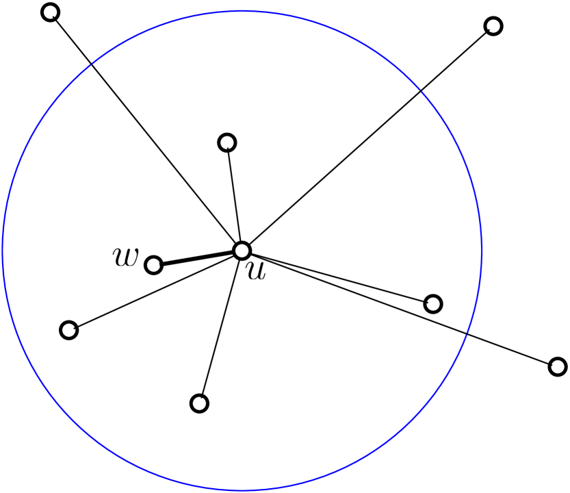
(a) Exchange Phase: edges connect $u$ with elements of $U_{u}$. Some of them can be “removed” in Filtering Phase.

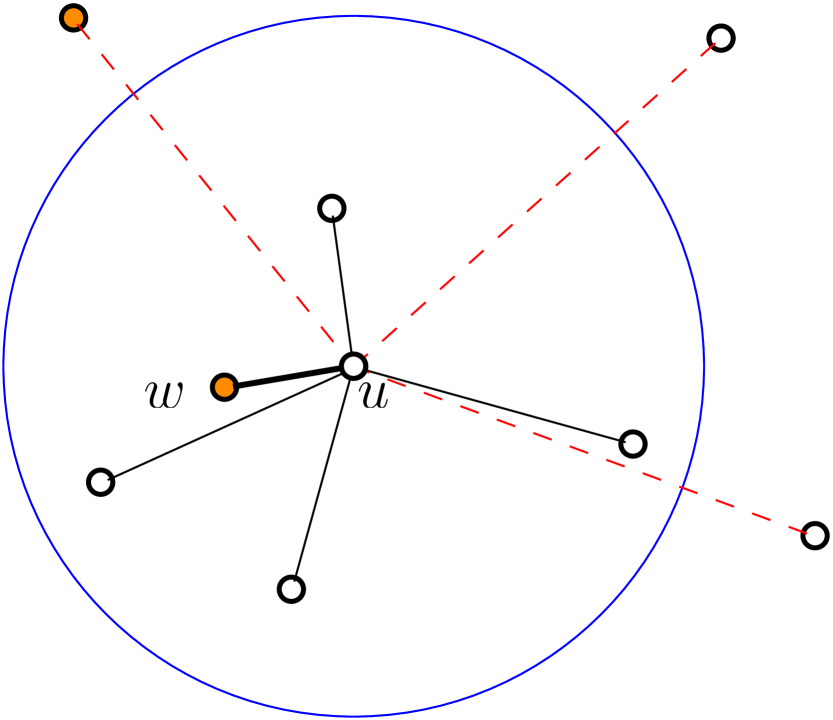
(b) Filtering Phase: If $u$ hears some node $w$, it can “remove” all other nodes that transmitted in that round. The dashed edges denote nodes removed for sure.

(c) A possible result of the proximity graph construction. Only close pairs are guaranteed to be connected by an edge.

Figure 3: An illustration of the proximity graph construction (Algorithm 1). The blue circle contains $\kappa$ closest nodes to $u$.

4 Network sparsification and its applications

In this section we describe a sparsification algorithm which decreases density of a network by removing some nodes from dense areas and assigning them to their “parents” which are not removed. Simultaneously, the algorithm builds a schedule in which removed nodes exchange messages with their parents. Using sparsification as a tool, we develop other tools for (non)sparsified networks. Finally, a clustering algorithm is given which partitions a network (of awaken nodes) into clusters in time independent of the diameter of a network.

4.1 Sparsification

A $c$-sparsification algorithm for a constant $c\leq 1$ is a distributed ad hoc algorithm $S$ which, executed on a set of nodes $X$ of density $\Delta\leq N$, determines a set $Y\subseteq X$ such that:

1. density of $Y$ is at most $c\Delta$,

2. each $v\in X$ knows whether $v\in Y$ and each $v\in X\setminus Y$ has assigned $\text{parent}(v)\in Y$ such that $v$ and parent$(v)$ exchange messages during an execution of $S$ on $X$.

Moreover, if $X$ is a clustered set, cluster$(v)$=cluster$(\text{parent}(v))$ for each $v\in X\setminus Y$.

Alg. 2 contains a pseudocode of our sparsification algorithm. The algorithm builds a proximity graph of a network several times. Each time a proximity graph $H$ is determined, an independent set $Y$ of $H$ is computed such that:

• for each dense cluster $\phi$, at least one element of $\phi$ is in $Y$ (clustered case) or

• for each dense unit-ball ${\mathcal{B}}$, there is an element in $Y$ located close to the center of ${\mathcal{B}}$ (unclustered case).

Then, some elements of $Y$ are linked with their neighbours in $Y$ by parent/child relation and removed from the set of nodes attending consecutive executions of ProximityGraphConstruction.

(a) Clustered case. Child-parent relations is possible only between nodes of the same cluster.

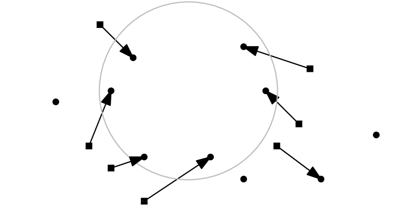
(b) Unclustered case. An example demonstrates that the number of nodes in a dense unit ball (in gray) is not necessarily reduced, due to the fact that all nodes from the ball become parents of nodes outside of the ball.

Figure 4: An example of sparsification of a network. Each edge corresponds to child-parent relation (the direction of an edge is from a child to its parent). The elements of the returned set of nodes are denoted by dots, the remaining nodes are denoted by squares.

In this way, the density of the set of nodes attending the algorithm gradually decreases. Details of implementation of the algorithm, including differences between clustered and unclustered variant, and analysis of its efficiency are presented below (see also Fig. 4).

Algorithm 2 Sparsification$(\Gamma,X)$

1:For each $v\in X$: parent$(v)=\bot$, children$(v)=\emptyset$

2:$\text{Active}\leftarrow X$, $\text{Prnts}\leftarrow\emptyset$, $\text{GlobChl}\leftarrow\emptyset$

3:for $i=1,2,\ldots,\Gamma$ do

4:    $H\leftarrow$ ProximityGraphConstruction$(\text{Active})$

5:     $Y\leftarrow\text{IndependentSet}(H)$$\triangleright$ Implementions different for clustered/unclustered $X$

6:    $\text{NewChl}\leftarrow\{v\in\text{Active}\,|\,v\not\in Y\mbox{ and }N_{v}^{H}\cap Y\neq\emptyset\}$$\triangleright$ $N_{v}^{H}$ denotes the set of neighbors of $v$ in $H$

7:    for each $v\in\text{NewChl}$ do

8:         parent$(v)\leftarrow\min(N_{v}^{H}\cap Y)$

9:         $\text{children}(\text{parent}(v))\leftarrow\text{children}(\text{parent}(v))\cup\{v\}$     

10:    $\text{Prnts}\leftarrow\text{Prnts}\cup\{v\in\text{Active}\,|\,\text{children}(v)\neq\emptyset\}$

11:    $\text{GlobChl}\leftarrow\text{GlobChl}\cup\text{NewChl}$

12:    $\text{Active}\leftarrow\text{Active}\setminus(\text{Prnts}\cup\text{GlobChl})$

13:return $\text{Active}\cup\text{Prnts}$

For a clustered network, IndependentSet$(G)$ is chosen as the set of local minima in a proximity graph, that is, $Y\leftarrow\{v\,|\,\text{ID}(v)<\min(\{\text{ID}(u)\,|\,u\in N_{v}^{H}\})\}.$

Lemma 8:

Alg. 2 is a $\frac{3}{4}$-sparsificaton algorithm for clustered networks, it works in time $O(\Gamma\log N)$.

Proof.

First, let us discuss an implementation of the algorithm in a distributed ad hoc network. A proximity graph $H$ is built by Alg. 1 in $O(\log N)$ rounds. Moreover, after an execution of Alg. 1, all nodes know their transmission patterns in the schedule $S$ of length $O(\log N)$ such that each pair of neighbors $u,v$ in $G$ exchange messages during $S$. Therefore, each node $v$ knows its neighbors $N_{v}^{H}$ in $H$ as well. In order to execute the remaining steps in the for-loop, nodes determine locally whether they belong to NewChl. Then elements of NewChl choose their parents and send messages to them using the schedule $S$. Simultaneously, each node updates the local children$(v)$ variable if it receives messages from its new child(ren). (Note that a directed graph connecting children with their parents is acyclic.

Lemma 7 implies that the graph $H$ built by ProximityGraphConstruction connects by an edge each close pair. Thus, by Lemma 1.2, $H$ contains at least one edge connecting elements of $\phi$, for each dense cluster $\phi$. Thus, $Y$ contains at least one element of $\phi$ and, since edges connect only nodes of the same cluster, at least one element of $\phi$ determines its parent inside $\phi$. As the result, at least two elements of $\phi$ are removed from Active in each execution of ProximityGraphConstruction.

These properties guarantee that each repetition of the main for-loop decreases the number of elements of Active in each dense cluster. Therefore, each cluster contains at most $\Gamma/2$ elements of Active after $O(\Gamma)$ repetitions of the loop.

Let $\text{Active}^{\prime}$, $\text{Prnts}^{\prime}$, $\text{GlobChl}^{\prime}$ be the intersections of Active, Prnts and GlobChl with a cluster $\phi$. Above, we have shown that $|\text{Active}^{\prime}|\leq\Gamma/2$, while the algorithm returns $\text{Active}^{\prime}\cup\text{Prnts}^{\prime}$. Thus, in order to prove the lemma, it is sufficient to show that $|\text{Prnts}^{\prime}|\leq\Gamma/4$. For each cluster $\phi$, each element of $\text{Prnts}^{\prime}$ from this cluster has assigned nonempty subset of the cluster as children of $v$ and the sets of children of nodes are disjoint. Thus, the number of elements of $\text{Prnts}^{\prime}$ in the cluster is at most as large as the number of elements of $\text{GlobChl}^{\prime}$ in that cluster: $|\text{Prnts}^{\prime}|\leq|\text{GlobChl}^{\prime}|$. Summing up, $|\text{Active}^{\prime}\cup\text{Prnts}^{\prime}\cup\text{GlobChl}^{\prime}|\leq\Gamma$, $|\text{Active}^{\prime}|\leq\Gamma/2$, $|\text{Prnts}^{\prime}|\leq|\text{GlobChl}^{\prime}|$. As $\text{Active}^{\prime}$, $\text{Prnts}^{\prime}$, and $\text{GlobChl}^{\prime}$ are disjoint, the finally returned set $\text{Active}^{\prime}\cup\text{Prnts}^{\prime}$ contains at most $\frac{3}{4}\Gamma$ elements from the considered cluster $\phi$. ∎

For unclustered networks IndependentSet$(G)$ is determined by a simulation of the distributed Maximal Independent Set (MIS) algorithm for the LOCAL model [34] which, for graphs of constant degree, works in time $O(\log^{*}n)$ and sends $O(\log n)$-size messages. As ProximityGraphConstruction builds an $O(\log N)$ time schedule in which each pair of neighbors $u,v$ (of a built proximity graph) exchange messages, we can simulate each step of the algorithm from [34] in $O(\log N)$ rounds. In contrast to the clustered networks, we are unable to guarantee that a single execution of Sparsification reduces the density in an unclustered network. This is due to the fact that a node from dense unit ball might become a parent of a node outside of this ball (see Fig. 4(b)); as a result the number of elements in the considered unit ball is not reduced during an execution of Sparsification. Therefore, we have to deal with unclustered case more carefully. Let $l\leftarrow\chi(5,1-\varepsilon)$ and let SparsificationU$(\Gamma,X)$ be an algorithm which executes Sparsification$(\Gamma,X_{i})$ for $i=0,\ldots,l-1$, where $X_{0}=X$, $X_{i}$ is the set returned by Sparsification$(\Gamma,X_{i-1})$ and $X_{l}$ is the set returned as the final result.

Algorithm 3 SparsificationU$(\Gamma,X)$

1:$X_{0}\leftarrow X$

2:$l\leftarrow\chi(5,1-\varepsilon)$

3:for $i=0,\ldots,l-1$ do

4:    $X_{i+1}\leftarrow$ Sparsification$(\Gamma,X_{i})$

5:    $S_{i}$: the schedule of Sparsification$(\Gamma,X_{i})$

6:return $(X_{1},\ldots,X_{l})$, $(S_{0},\ldots,S_{l-1})$

Lemma 9:

An execution of SparsificationU$(\Gamma,U)$ on an unclustered set $U$ of density $\Gamma$ returns a sequence of set $X_{0}\supseteq X_{1}\supseteq\cdots\supseteq X_{l}$ and schedules $S_{0},\ldots,S_{l-1}$ such that the density of $X_{l}$ is at most $\frac{3}{4}\Gamma$, each node $x\in X_{i}\setminus X_{i+1}$ exchange messages with parent$(x)\in X_{i+1}$ during $S_{i}$. Morover, SparsificationU$(\Gamma,U)$ works in time $O(\Gamma\log N\log^{*}N)$.

Proof.

The analysis of the sparsification algorithm for clustered networks relies on the fact that there is a close pair in each dense cluster $\phi$ and therefore the number of active elements in $\phi$ is reduced after each iteration of the for-loop in Alg. 2. In the unclustered network, it might be the case that there is no close pair in a dense unit-ball. That is why the reasoning from Lemma 8 does not apply here.

We define an auxiliary notion of saturation. For a unit ball ${\mathcal{B}}=B(x,1)$, the saturation of ${\mathcal{B}}$ with respect to the set of nodes $X$ is the number of elements of $X$ in $B(x,5)$. As long as ${\mathcal{B}}$ contains at least $\Gamma/2$ nodes in an execution of ProximityGraphConstruction, there is a close pair $u,v$ in $B(x,5)$ (Lemma 1) and therefore $u,v$ are connected by an edge in $H$. Thus, $u$ or $v$ is not in the computed MIS (line 5); wlog assume that $u$ is not in MIS. Thus, $u$ is dominated by a node from MIS and therefore it becomes a member of GlobChl and it is switched off. This in turn decreases saturation of $B(x,5)$. Thus, an execution of Sparsification results either in decreasing the number of nodes in ${\mathcal{B}}$ to $\leq\Gamma/2$ or in reducing saturation of ${\mathcal{B}}$ by at least $\Gamma$. As $B(x,5)$ might be covered by $l=\chi(5,1)$ unit balls, there are at most $l\Gamma$ nodes in $B(x,5)$ and saturation can be reduced at most $l\Gamma$ times. Hence, $l$ repetitions of Sparsification eventually leads to the reduction of the number of active elements located in ${\mathcal{B}}$ to $\leq\Gamma/2$. ∎

4.2 Full Sparsification

A full sparsification algorithm is a distributed ad hoc algorithm/schedule $S=S_{1}S_{2}\ldots S_{k}$ which, executed on an $r$-clustered set of nodes $A$ of density $\Gamma$ determines sets $A_{0},A_{1},\ldots,A_{k}$ such that $k=\log_{4/3}\Gamma$, $A_{i+1}\subseteq A_{i}$ (each node $v\in A$ knows whether $v\in A_{i}$), $A_{0}=A$ and, for each $i\in[k]$:

1. the density of $A_{i}$ is at most $\max\{\Gamma(3/4)^{i},\chi(r,1-\varepsilon)\}$,

2. for each cluster $\phi$ present in $A$, $A_{k}$ contains at least one element of $\phi$,

3. each $v\in A_{i}\setminus A_{i+1}$ has assigned $\text{parent}(v)\in A_{i+1}$ such that $v$ and parent$(v)$ exchange messages during $S_{i}$ and cluster$(v)$=cluster$(\text{parent}(v))$.

Alg. 4 contains a pseudocode of our full sparsification algorithm (see also Fig. 5). In Lemma 10, the properties of this algorithm (following directly from Lemma 8) are summarized.

Algorithm 4 FullSparsification$(\Gamma,A)$

1:$A_{0}\leftarrow A$,

2:$X\leftarrow A$, $\Lambda\leftarrow\Gamma$, $k\leftarrow\log_{\frac{3}{4}}\Gamma$

3:for $i=1,2,\ldots,k$ do

4:    $Y\leftarrow\text{Sparsification}(\Lambda,X)$

5:    $S_{i}\leftarrow$ the schedule of $\text{Sparsification}(\Lambda,X)$

6:    $A_{i}\leftarrow X\setminus Y$

7:    $X\leftarrow Y$

8:    $\Lambda\leftarrow\frac{3}{4}\Lambda$

9:return $(A_{0},\ldots,A_{k}),(S_{1},\ldots,S_{k})$

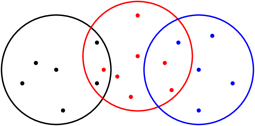
(a) The clustered set $A$, where colors correspond to clusters.

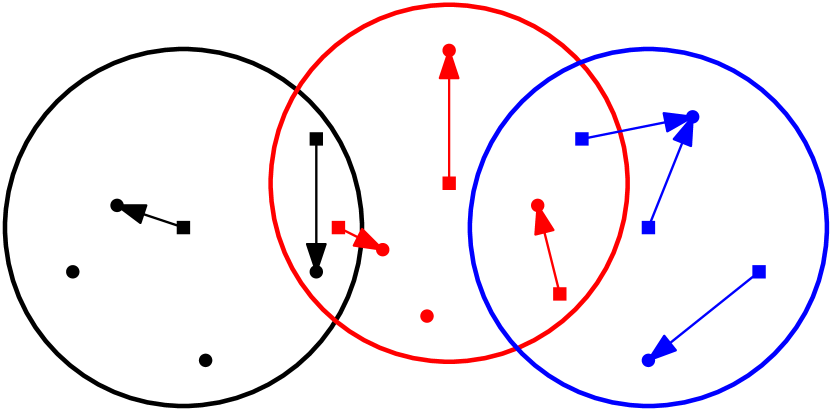
(b) The result of the first execution of Sparsification. Nodes from $A_{1}$ are denoted by squares.

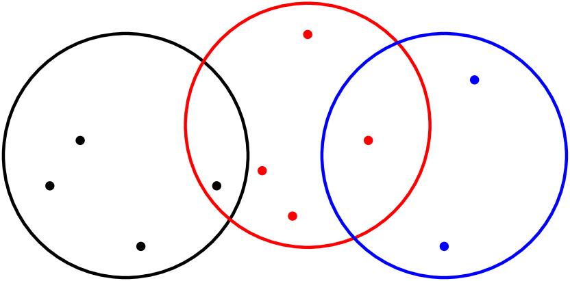
(c) The result of the second execution of Sparsification. Nodes from $A_{2}$ are denoted by empty squares.

Figure 5: An illustration of full sparsification. Each edge correspond to child-parent relation (the direction of an edge is from a child to its parent).

(a) The clustered set $A$, where colors correspond to clusters.

(b) The result of the first execution of Sparsification. Nodes from $A_{1}$ are denoted by squares.

(c) The set on which Sparsification is executed for the second time (dots from Figure (b)).

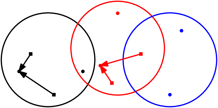
(d) The result of the second execution of Sparsification. Nodes from $A_{2}$ are denoted by squares.

Figure 6: An illustration of full sparsification. Each edge correspond to child-parent relation (the direction of an edge is from a child to its parent).

Lemma 10:

Algorithm 4 is a full sparsificaton algorithm for clustered networks which works in time $O(\Gamma\log N)$.

4.3 Imperfect labelings of clusters

Using $r$-clustering of a set $X$ with density $\Gamma$, it is possible to build efficiently an imperfect $c$-labeling of $X$, where $c$ is a constant which depends merely on $r$ and SINR parameters.

Lemma 11:

Assume that an $r$-clustering of a set $X$ of density $\Gamma$ is given. Then, it is possible to build $c$-imperfect labeling of $X$ in $O(\Gamma\log N)$ rounds, where $c$ depends merely on $r$ and SINR parameters.

Proof.

Let $S=S_{1},\ldots,S_{k}$ and $A_{1},\ldots,A_{k}$ be the schedules and the sets obtained as the result of an execution of FullSparsification$(\Gamma,X)$. FullSparsification$(\Gamma,X)$ splits each cluster in $O(1)$ trees, defined by the child-parent relation build during an execution of FullSparsification. (Indeed, the elements of $A_{k}$ are the roots of the trees.) The schedule $S$ (and its reverse $S^{R}$) of length $O(\Gamma\log N)$ allows for bottom-up (top-down) communication inside these trees. Using $S$ and $S^{R}$ one can implement tree-labeling algorithm as follows. First, each node learns the size of its subtree in a bottom-up communication. Then, the root starts top-down phase, where each node assigns the smallest label in a given range to itself and assigns appropriate subranges to its children. More precisely, the root starts from the range $[1,m]$, where $m$ is the size of the tree. Given the interval $[a,b]$, each node assigns $a$ as its own ID and splits $[a+1,b]$ into its subtrees. ∎

4.4 Reduction of radius of clusters

In this section we show how to reduce the radius of a clustering. Given an $r$-clustering of a set $X$ of density $\Gamma$, our goal is to build an $1$-clustering of $X$. The idea is to repeat the following steps several times. First, $X$ is fully sparsified, i.e., $O(1)$ nodes remain from each non-empty cluster. Then, a minimum independent set (MIS) of this sparse set is determined on the graph with edges $(u,v)$ connecting $u$, $v$ which exchange messages during an execution of Sparse Network Schedule (see Lemma 4). The elements of MIS become the centers of new clusters in the new $1$-clustering and they execute Sparse Network Schedule. A node $v$ (not in MIS) which receives a message from $w$ during this execution of SNS, becomes an element of $\text{cluster}(w)$ and it is removed from further consideration. As we show below, a $1$-clustering of $X$ can be obtained in this way efficiently by Alg. 5.

Algorithm 5 RadiusReduction$(\Gamma,X,r)$

1:For each $v\in X$: newcluster$(v)\leftarrow\bot$ $\triangleright$ $\bot$ means “undetermined”

2:for $i=1,2,\ldots,\chi(r+1,1-\varepsilon)$ do

3:    $(X_{0},\ldots,X_{k}),(S_{0},\ldots,S_{k})\leftarrow$ FullSparsification$(\Gamma,X)$

4:    Execute Sparse Network Schedule $L_{\gamma}$ from Lemma 4 on $X_{k}$

5:    Let $G(Y,E)$, where $E=\{(u,v)\,|\,u,v\text{ exchange messages during }L_{\gamma}\}$ and $Y=\{v\,|\,\exists_{u}\ (u,v)\in E\}$

6:     $D\leftarrow\text{MIS}(G)$ $\triangleright$ simulation of maximal independent set alg. from [34]

7:     Execute Sparse Network Schedule $L_{\gamma}$ from Lemma 4 on $D$ $\triangleright$ Local Broadcast from $D$, using L. 4

8:    for each $v\in X\setminus D$ do

9:         if $v$ received a message from $u\in D$ during execution of $L_{\gamma}$ in line 7 then

10:             $\text{newcluster}(v)\leftarrow u$$\triangleright$ Choose arbitrary $u$ if $v$ received many messages              

11:    $X\leftarrow X\setminus(D\cup\{v\,|\,\text{newcluster}(v)\neq\bot\})$

Lemma 12:

Assume that a $r$-clustering of a set $X$ of density $\Gamma$ is given for a fixed constant $r\geq 1$. Then, Algorithm 5 builds $1$-clustering of $X$ in $O((\Gamma+\log^{*}N)\log N)$ rounds.

Proof.

By Lemma 8, the set $X_{k}$ has density $c^{\prime}=O(1)$ and it contains at least one element from each nonempty cluster of $X$. Each pair of nodes from $X_{k}$ in distance $\leq 1-\varepsilon$ exchange messages during step 4, therefore the graph $G$ contains the communication graph of $X_{k}$. As $D$ computed in step 6 is a MIS of $X_{k}$ in the graph $G$ and $X_{k}$ contains at least one element from each nonempty cluster, there is an element of $D$ in close neighborhood of each cluster. More precisely, for a dense cluster $\phi$ with nodes located inside $B(x,r)$, there is an element of the computed maximal independent set (MIS) in $B(x,r+1)$. Indeed, by Lemma 10, there is $y$ from $\phi$ in $Y$. Thus, $y\in B(x,r)$, where $x$ is the center of the cluster $\phi$. Either $y$ is in the computed MIS or $y$ is in distance $\leq 1$ from an element $z$ from the MIS. In the latter case, $z\in B(x,r+1)$. Then, steps 7–10 assign all nodes in distance $\leq 1-\varepsilon$ (and some in distance $\leq 1$) from elements of $D$ (including the above defined $y$ or $z$) to new clusters included in unit balls with centers at the elements of $D$. Thus, the nodes from each “old” cluster are assigned to new clusters after $\chi(r+1,1-\varepsilon)$ repetitions of the main for-loop. ∎

4.5 Clustering algorithm

In this section we provide an algorithm which, given an unclustered set $A$, builds a $1$-clustering of $A$. The algorithm consists of two main parts. In the former part, the sequence of sets $A_{0}\supseteq\cdots\supseteq A_{kl}$ is built using SparsificationU, for $k=\log_{4/3}\Gamma$ and $l=\chi(5,1-\varepsilon)$. By Lemma 9, the density of $A_{il}$ is at most $\Gamma(\frac{3}{4})^{i}$. Moreover, a sequence of schedules $S_{0},\ldots,S_{kl}$ is built such that each $v\in A_{i}\setminus A_{i+1}$ exchange messages with parent$(v)\in A_{i+1}$. In the latter part, we start from $1$-clustering of $A_{kl}$, which is obtained by assigning each node $v\in A_{kl}$ to a separate cluster. Then, given an $1$-clustering of $A_{i}$ for $i>0$, we get $2$-clustering of $A_{i-1}$ by executing $S_{i-1}$ with messages equal to cluster IDs of transmitting nodes. The elements of $A_{i-1}$ choose clusters of their parents. Using RadiusReduction (Lemma 12), the obtained $2$-clustering is transformed into an $1$-clustering. A pseudocode is presented in Alg. 6.

Algorithm 6 Clustering$(\Gamma,A)$

1:$k\leftarrow\log_{4/3}\Gamma$

2:$X\leftarrow A$, $A_{0}\leftarrow A$

3:$\Lambda\leftarrow\Gamma$, $k\leftarrow\log_{\frac{3}{4}}\Gamma$, $l\leftarrow\chi(5,1-\varepsilon)$

4:for $i=1,2,\ldots,k$ do

5:    $(A_{(i-1)l+1},\ldots,A_{il}),(S_{(i-1)l+1},\ldots,S_{il})\leftarrow\text{SparsificationU}(\Lambda,X)$

6:    $X\leftarrow A_{il}$

7:    $\Lambda\leftarrow\frac{3}{4}\Lambda$

8:For each $v\in A_{kl}$: cluster$(v)\leftarrow\text{ID}(v)$

9:$X\leftarrow A_{kl}$

10:$\Lambda\leftarrow 1$

11:for $i=0,1,2,\ldots,kl$ do

12:    Execute $S_{kl-i}$, on $A_{kl-i}$, each $v\in A_{kl-i}$ sends cluster$(v)$ during the execution

13:    For each $v\in A_{kl-i-1}$: cluster$(v)\leftarrow\text{cluster}(\text{parent}(v))$

14:    $X\leftarrow X\cup A_{kl-i-1}$

15:    RadiusReduction$(\Lambda,X,2)$

16:    if $i\text{ mod }l=0$ then $\Lambda\leftarrow\frac{4}{3}\cdot\Lambda$

Theorem 1:

The algorithm Clustering builds $1$-clustering of an unclustered set $A$ of density $\Gamma$ in time $O(\Gamma\log N\log^{\star}N)$.

Proof.

Correctness of the algorithm follows from the properties of SparsificationU and RadiusReduction (Lemmas 9 and 12). The time of executions of SparsificationU is O(∑_i=1^k Γ(34)^ilogNlog^* N)=O(ΓlogNlog^*N). The time of executions of RadiusReduction is O(∑_i=1^k (Γ(34)^i+log^*N)⋅logN)=O(ΓlogN+log^*NlogN). Altogether, time complexity is $O(\Gamma\log N\log^{\star}N)$. ∎

5 Communication problems

In this section, we apply sparsification and clustering in distributed algorithms for broadly studied communication problems, especially the local and global broadcast.

5.1 Local broadcast

Now, we can solve the local broadcast problem for a set $V$ of density $\Delta$ by the following LocalBroadcast algorithm.

Algorithm 7 LocalBroadcast($V,\Delta$)

1:Clustering($\Delta,V$) $\triangleright$ Theorem 1

2:Imperfect labeling of $V$ $\triangleright$ Lemma 11

3:for $l=1,\ldots,\Delta$ do

4:    Run SNS on nodes with label equal to $l$ $\triangleright$ Lemma 4

First, the clustering algorithm is applied which builds a $1$-clustering of $V$ in time $O(\Delta\log N\log^{\star}N)$ (Theorem 1). Then, an imperfect labeling of clusters can be formed in time $O(\Delta\log N)$ (Lemma 11). Finally, an algorithm which executes $\Delta$ times Sparse Network Schedule (see Lemma 4), the $l$th execution of SNS is performed by the nodes with label $l$. As each label appears $O(1)$ times in each cluster, the density of the set of nodes with label $l$ (for each $l$) is $O(1)$ for each $l\in[N]$. Thus, consecutive executions of SNS accomplish the local broadcast task (see Lemma 4).

Theorem 2:

The algorithm LocalBroadcast performs local broadcast from a set $V$ of density $\Delta$ in time $O(\Delta\log N\log^{\star}N)$.

In this section we present an algorithm for the local broadcast problem. The key idea is to select a sparse subset $\mathcal{L}$ of nodes that forms an independent set in the communication graph and run the broadcast process starting in each of the nodes of $\mathcal{L}$. Due to Proposition LABEL:p:stage2 we have that all nodes that are in an internal state transmit a message to all the neighbors. After the broadcast is finished all nodes are in state $\mathcal{I}$. We exploit this property to perform local broadcast. However, the number of rounds needed for the broadcast process is dependent on the maximal distance from any node $v$ to the closest node $w\in\mathcal{L}$. Formally, let $d^{*}=\max_{v\in G}\min_{w\in\mathcal{L}}d(v,w)$, then it is sufficient to run $d^{*}+1$ phases of the broadcast algorithm. This yields a complexity of $O(d^{*}(\Delta+\log^{*}n)\log n)$. We construct the network sparsification $\mathcal{L}$ such that $d^{*}=O(\log n)$ and the complexity of our local broadcast algorithm is $O((\Delta+\log^{*}n)\log^{2}n)$.

Network Sparsification. We call a set $\mathcal{L}$ of nodes a network sparsification if it satisfies the following criteria. The elements of the set are called leaders.

• For each $u,w\in\mathcal{L}$ we have $d(u,w)>1-\varepsilon$.

• For any $v\not\in\mathcal{L}$ there is a leader $w\in\mathcal{L}$ such that $d(v,w)\leq\log n$.

The idea to generate such sparsification is to use a BuildTree-like procedure (see Algorithm LABEL:alg:build_tree) to organize nodes into trees and designate the roots to become the leaders. However, there is a major caveat to this: MonoGraphConstruction – the key routine used in TreeMerging Algorithm assumes preexisting clustering of the network. Namely, each node $v$ has to be assigned to some cluster (indicated by the $\operatorname{ref}(v)$ variable). In the broadcast algorithm it was realized by coupling nodes assigned to the same master node into one cluster. Unlike the broadcast scenario no nodes are assumed to be distinguished at the beginning of local broadcast. Since we do not have any initial clustering we redesign the procedure to work on unclustered networks at the cost of larger spread of trees – that is, we allow for a tree to occupy area of diameter $O(\log n)$ instead of $O(1)$.

The presented algorithm organizes a network in trees of depth at most $\log n$ such that for each two trees their roots are within distance at least $1-\varepsilon$. The trees are built in a similar way to the communication trees (see Algorithm LABEL:alg:build_tree). However, we adjust TreeMerging (Algorithm LABEL:alg:treemerging) subroutine to take into the account the rank (the size of a tree rooted at the node), so that node with lower rank joins the node with higher rank. This makes the rank of the parent at least twice the rank of its children, thus bounds the depth of a tree by $O(\log n)$.

Algorithm 8 NewTreeMerging$(\Gamma)$ in node $v$

1:counter $\leftarrow 0$, $\operatorname{ref}(v)\leftarrow 0$

2:while parent$(v)=\bot$ and counter $<\Gamma$ do

3:    counter $\leftarrow$ counter$+1$

4:    $H\leftarrow$ ProximityGraphConstruction$(v)$

5:    Compute Maximal Independent Set of $H$

6:    If $v$ has no neighbours then wait until the next iteration of while loop.

7:    if $v\in MIS(H)$ then

8:         Transmit message $\langle v,\text{MISNode}\rangle$

9:         Let $K=\{v_{1},...,v_{k}\}$ be the set of nodes that sent handshake message to $v$.

10:         Choose any $w\in K$

11:         if rank$(w)>$ rank$(v)$ then

12:             Send a parent declaration message $\langle w,v,\text{rank}(v)\rangle$

13:             parent$(v)\leftarrow w$

14:         else

15:             Send a message of acceptance $\langle v,w\rangle$.

16:             children$(v)\leftarrow$ children$(v)\cup\{w\}$

17:             rank$(v)\leftarrow$ rank$(v)+$ rank$(w)$          

18:    else

19:         Let $L$ be the set of received messages of type $\langle w,\text{MISNode}\rangle$.

20:         if $L$ is non-empty then

21:             Let $u$ be the node such that $\langle u,\text{MISNode}\rangle\in L$ having minimal ID.

22:             Transmit a handshake message $\langle u,v,\text{rank}(v)\rangle$.

23:             if received an acceptance message from $u$ then

24:                 parent$(v)\leftarrow u$

25:             else if received a parent declaration message from $u$ then

26:                 children$(v)\leftarrow$ children$(u)\cup\{u\}$

27:                 rank$(v)\leftarrow$ rank$(v)+$ rank$(u)$                           

The line of proof of correctness and complexity is the same as for TreeMerging Algorithm, however some details must be explained. The main idea was to show that in each iteration of the main while-loop, in every dense region, at least two trees merge. To carry this analysis we argue that in every dense region graph $H$ has at least one edge. This is true due to fact that in every such area there must be a locally minimal pair of nodes that hear each other (cf. Lemma LABEL:l:monograph) during ProximityGraphConstruction. Then, at least one node near the edge is selected to $MIS(H)$ and coordinates the tree merging. This concludes the sketch of proof supplement to the correctness of the algorithm.

Local Broadcast via Broadcast. Now, we have all the pieces to perform local broadcast. After running a version of BuildTree algorithm, adjusted as described in previous subsection, we obtain a network sparsification – $\mathcal{L}$ in which we initiate the broadcast algorithm which terminates after $O((\Delta+\log^{*}n)\log^{2})$ rounds. Thanks to its properties we know that all nodes had a chance to transmit a message to all its neighbors (see Proposition LABEL:p:stage2), and thus complete the task of local broadcast.

Theorem 3:

Running the broadcast algorithm with a set of sources $\mathcal{L}$ solves local broadcast problem in $O((\Delta+\log^{*}n)\log^{2})$ rounds.

5.2 Sparse multiple-source broadcast

In this section we consider sparse multiple source broadcast (SMSB) problem, a generalization of the global broadcast problem. This generalization is introduced for further applications for other communication problems as leader election and wake-up.

The sparse multiple source broadcast problem (SMSB problem) is defined as follows. At the beginning, the unique broadcast message is known to a set of distinguished nodes $S\subset V$ such that $d(u,v)>1-\varepsilon$ for each $u,v\in S$, $u\neq v$. The problem is solved when

1. the broadcast message is delivered to all nodes of the network, AND

2. each node $v\in V$ transmitted a message in some round which was received by all its neighbors in the communication graph.

The algorithm for SMSB problem. Let $V_{i}$ denote the set of nodes in the graph-distance $i$ from $S$, i.e., $v\in V_{i}$ if a shortest path from an element of $S$ to $v$ has length $i$. The algorithm works in phases. In Phase 1, Sparse Networks Schedule (Lemma 4) is applied on the set of distinguished nodes $S$. In this way all elements of $S$ transmit messages received by $V_{1}$, their neighbors in the communication graph (and possibly some other nodes in geometric distance at most $1$). After receiving the first message from $s\in S$, a node $v\in V\setminus S$ assigns itself to the cluster $s$. Hence, the set of awaken nodes $L_{1}$ contains $V_{1}$ and we have $1$-clustering of $L_{1}$.

In Phase $i>1$, local broadcast is executed on $L_{i}$, the set of nodes awaken in Phase $i-1$ . In this way, the set of nodes awaken in the first $i$ phases contains all nodes in graph distance $i$ from $S$, i.e., $\bigcup_{j\in[i]}V_{j}\subseteq\bigcup_{j\in[i]}L_{j}$. Moreover, we assure that all nodes awaken in a phase are $1$-clustered at the end of the phase. (Thus, each node knows its cluster ID in such clustering).

A phase consists of three stages. In Stage 1 of phase $i$, an imperfect labeling of each cluster of $L_{i}$ is built. This means that each node $v$ is assigned a label $l_{v}$ such that, for each cluster, the number of nodes with the same label in the cluster is $O(1)$(see Lemma 11). In Stage 2, Sparse Network Schedule (Lemma 4) is executed $\Delta$ times. A node with label $l$ participates in the $l$th execution of SNS only. In this way, all nodes from $L_{i}$ transmit on distance $1-\varepsilon$. All nodes awaken in Stage 2 inherit cluster numbers from nodes which awaken them. In this way, we obtain a $2$-clustering of $L_{i+1}$, the set of nodes awaken in Stage 2. The goal of Stage 3 is (given the obtained $2$-clustering) to build an $1$-clustering of awaken nodes. (See Fig. 1 in Section 1 for an example.)

Algorithm 9 SMSBroadcast($V,S$)

1:SNS($S$)

2:$L_{1}\leftarrow$ nodes awaken by elements of $S$, clustered by IDs of their neighbors from $S$

3:for $i=1,2,\ldots$ do

4:    Stage 1: imperfect labeling of $L_{i}$ $\triangleright$ Lemma 11

5:    Stage 2: local broadcast from $L_{i}$, using assigned labels $\triangleright$ Lemma 4

6:$\triangleright$ Awaken nodes form $L_{i+1}$ and inherit cluster IDs from nodes which awaken them.

7:    Stage 3: RadiusReduction($\Delta,L_{i+1},2$) using $2$-clustering given by inherited cluster numbers

8:$\triangleright$ Lemma 12.

Using Lemmas 11, 4 and 12, we obtain the following result.

Theorem 4:

Algorithm SMSBroadcast solves sparse multiple source broadcast problem in $O(D(\Delta+\log^{*}N)\log N)$ rounds. For $S$ of size $1$, the algorithm solves the global broadcast problem.

5.3 Other problems

By applying the clustering algorithm and SMSBroadcast, solutions for other widely studied problems can be obtained, e.g., leader election or wake-up. Examples of such solutions are presented in Appendix, Section LABEL:s:app:other. By applying the clustering algorithm and SMSBroadcast, solutions for other widely studied problems can be obtained, e.g., leader election or wake-up.

Wake-up problem In the wake-up problem [23], some nodes become spontaneously active at various rounds and the goal is to activate the whole network. Nodes which do not become active spontaneously can be activated by a message successfully delivered to them. Spontaneous wake-ups are controlled by an adversary, thus an algorithm solving the problem should work for each pattern of spontaneous activations. A node can not participate in an execution of an algorithm as long as it is not active. Time of an execution of a wake-up algorithm is the number of rounds between the spontaneous activation of the first node and the moment when all nodes are activated. We assume the model with global clock, i.e., there is a central counter of rounds and each node knows the current value of that counter.

For a while, assume that all spontaneous wake-ups appear at the same round $r$. Then, starting at round $r$, we call Clustering (Alg. 6) on the set of spontaneously awaken nodes $S$ (see Lemma 9). As a result, we get a nonempty set $S^{\prime}\subset S$ of constant density in $O(\Delta\log N\log^{*}N)$ rounds. Then, SMSBroadcast$(V,S^{\prime})$ activates all nodes on a network in $O(D(\Delta+\log^{*}N)\log N)$ rounds. Let $T(N,\Delta)=O(D(\Delta+\log^{*}N)\log N)$ be the exact number of rounds of this algorithm. In order to adjust the above algorithm to arbitrary times of spontaneous wake-ups, we start a separate execution of this algorithm at each round $r$ whose number is divisible by $T(N,\Delta)$. In an execution starting at round $r$, only nodes awaken before $r$ are considered to be activated spontaneously. Thus, we have the following result.

Theorem 5:

The wake-up problem in networks with global clock can be solved in $O(D(\Delta+\log^{*}N)\log N)$ rounds.

Leader election The leader election problem is to choose (exactly) one node in the whole network as the leader, assuming that nodes are awaken in various rounds. First, assume that all nodes start a leader election algorithm at the same round. In order to elect the leader, we first execute Clustering (Alg. 6) on all nodes of a network which takes $O(\Delta\log^{*}N\log N)$ rounds and determines the non-empty set $S$ of constant density. Then, a unique member of $S$ is chosen as the leader, in the following (standard) way. Observe that one can verify whether $S$ contains nodes with IDs in the range $[l,r]$ by executing SMSBroadcast$(V,S^{\prime})$, where $S^{\prime}$ are nodes from $S$ with IDs in $[l,r]$. Thus, it is possible to choose the leader from $S$ by binary search which starts from the range $[1,N]$ and requires $O(\log N)$ executions of SMSBroadcast. In order to adjust the above algorithm to arbitrary times of spontaneous wake-ups of nodes, we start a separate execution of the algorithm at each round $r$ whose number is divisible by $T(N,\Delta)$, where $T(N,\Delta)=O(D(\Delta+\log^{*}N)\log^{2}N)$ is the upper bound on the time of the algorithm. In an execution starting at round $r$, only nodes awaken before $r$ are considered to be activated spontaneously. Finally, we have the following result.

Theorem 6:

The leader election problem in networks with global clock can be solved in $O(D(\Delta+\log^{*}N)\log^{2}N)$ rounds.

6 Lower Bound

In this section we prove a lower bound on the number of rounds needed to perform global broadcast.

Theorem 7:

A deterministic algorithm for the global broadcast in the SINR network works in time $\Omega(D\Delta^{1-1/\alpha}+\Delta)$, provided $N=\Omega(D\Delta)$ and the connectivity parameter $\varepsilon>0$ is small enough.

In order to prove the above theorem, we build a family of networks called gadgets. Each network from the family consists of $\Delta+4$ nodes $s,v_{0},\ldots,v_{\Delta+1},t$ located on the line – see Fig. 7 (in Section 6) for locations and distances between nodes. Thus, in particular, $s$ is connected by an edge in the communication graph with $v_{0},\ldots,v_{\Delta+1}$, $t$ is connected merely with $v_{\Delta+1}$ and only messages from $v_{\Delta+1}$ can be received by $t$. One can show that, for each deterministic algorithm, one can assign IDs to the nodes $s,v_{0},\ldots,v_{\Delta+1}$ such that the broadcast message originating at $s$ will be delivered to $t$ after $\Omega(\Delta)$ rounds. For the purpose of the lower bound, the main property of the locations of nodes in the gadget are:

1. The node $v_{i}$ does not receive any message, provided at least two nodes from the set $\{v_{j}\,|\,j<i\}$ transmit at the same time.

2. The node $t$ can receive a message from $v_{\Delta+1}$ ($v_{\Delta+1}$ is the only node from the gadget in distance $\leq 1$ from $t$) only in the case that no other node from the gadget transmits at the same time.

Using (a), we assign IDs to consecutive nodes $v_{1},v_{2},\ldots$ such that, after $i$ rounds, the nodes $v_{k}$ for $k>2i$ do not have any information about their location inside the set $\{v_{l}\,|\,l>2i\}$. Thus, the only available information differentiating them are their IDs. As a result, we prevent a transmission of $v_{\Delta+1}$ in a round in which other nodes from the gadget do not transmit for $\Omega(\Delta)$ rounds.

A natural idea to generalize such a result to $\Omega(D\Delta)$ is to connect sequentially consecutive gadgets such that the target ($t$) of the $i$th gadget is identified with the source $s$ of the $(i+1)$st gadget. Such approach usually works in the radio networks model, where no distant interferences appear. However, under the SINR constraints, the interference from distant nodes might potentially help, since it differentiate history of communication for nodes in various locations (even the close ones). Therefore, the applicability of this idea under the SINR constraints is limited. Instead of identifying the target $t$ of the $i$th gadget with the source of the $(i+1)$st gadget $s$, we separate each two consecutive gadgets by a long “sparse” path of nodes such that consecutive nodes are in distance $1-\varepsilon$ (Fig. 9). In this way, we limit the impact of nodes located outside of a gadget on communication inside the gadget. Finally, our result is only $\Omega(D\Delta^{1-1/\alpha})$. Below, we give a full formal proof following the above ideas.

6.1 Proof of Theorem 7

First, we build a gadget (sub)network consisting of $\Delta+4$ nodes $s$, $v_{0},\ldots,v_{\Delta+1}$, $t$ located on the line – see Figure 7 and Figure 8 for locations of nodes of a gadget. The notion gadget denotes actually a family of (sub)networks with location of nodes described on Figure 7 and Figure 8 and aribtrary IDs in the range $[N]$. Observe that the diameter $D$ of the gadget network is equal to $2$ (indeed, $s$ is connected to $v_{0},\ldots,v_{\Delta+1}$, $(v_{i},v_{j})$ is and edge for each $i\neq j$ and $t$ is connected with $v_{\Delta+1}$). In Lemma 13 we show that any deterministic algorithm needs $\Omega(\Delta)$ rounds to deliver a message to $t$ (the target), which originally is known only to $s$ (the source). More precisely, we show that there exists an assignment of IDs for the nodes of the gadget such that delivery of a message from $s$ to $t$ takes $\Omega(\Delta)$ rounds. As our ultimate goal is to analyse networks which contain gadgets as subnetworks, we make an additional assumption that a limited interference from outside of the gadget might appear.

Figure 7: The gadget. The nodes $s$ and $t$ are called the source and the target of a given gadget. Importantly, $d(x,t)>1$ for each $x$ from the gadget except of $v_{\Delta+1}$.

Figure 8: The core of the gadget, $d(v_{i},v_{i+1})=\varepsilon/2^{\Delta-i}$ for $i<\Delta$. Observe, that $2\varepsilon<d(v_{0},v_{\Delta+1})<3\varepsilon$.

Lemma 13:

For any deterministic algorithm $\mathcal{A}$ there exists a choice of identifiers for the nodes in the gadget such that the following holds. Let $\nu$ be the number satisfying $\frac{P/(4\varepsilon)^{\alpha}}{{\mathcal{N}}+\nu}=\beta$ and let $I\subseteq[N]$ be a set of allowed IDs such that $|I|\geq\Delta+4$. Assume that the interference coming from the outside of the core of the gadget $G$ in any node of the core is smaller than $\nu$ in every round. Moreover, assume that $s$ is the only awake node of the gadget at a given starting round. Then, it takes $\Omega(\Delta)$ rounds until the broadcast message is delivered to $t$ using algorithm $\mathcal{A}$.

Proof.

The fact that the sequence of distances $d(v_{0},v_{1}),d(v_{1},v_{2}),\ldots$ forms a geometric sequence implies the following property, provided $\varepsilon>0$ is a small enough constant.

Fact 2:

1. If the nodes $v_{i}$ and $v_{j}$, for $i<j$ are transmitting in a round then the nodes $v_{j+1},...,v_{\Delta+1}$ do not receives a message in that round.

2. If $v_{\Delta+1}$ is not the only transmitter from the set $\{v_{0},\ldots,v_{\Delta+1}\}$ in a round, then $t$ does not receive a message in that round.

As $\{v_{0},\ldots,v_{\Delta+1}\}$ are asleep at the beginning, they are all awaken in a round in which $s$ sends its first message, thanks to the fact that interference from outside of the gadget’s core is bounded by $\nu$. In order to simplify notations, assume that the number of the round in which $v_{0},\ldots,v_{\Delta+1}$ receive the first message from $s$ is equal to $0$. Recall that $v_{\Delta+1}$ is the only node from the gadget that can pass a message to the target $t$ (c.f. Figure 7 and Figure 8). Our goal is to gradually assign IDs to $v_{0},v_{1},v_{2},\ldots$ such that, in each round $j\in[i/2]$,

• either no node from the set $\{v_{0},\ldots,v_{\Delta+1}\}$ transmits,

• or at least two nodes from $\{v_{0},\ldots,v_{i}\}$ transmit.

In this way the assignment of IDs prevents $v_{\Delta+1}$ from being the unique transmitter from $\{v_{0},\ldots,v_{\Delta+1}\}$ for $\Omega(\Delta)$ rounds. This fact in turn guarantees that $t$ does not receive any message in $\Omega(\Delta)$ rounds.

Now, we describe the process of assigning IDs to $v_{0},\ldots,v_{\Delta+1}$. Let $I_{0}=I$ of size $\geq\Delta+4$ be the set of allowed IDs at the beginning.

Let $r_{0}^{i}>0$ be the smallest round number in which the node with ID equal to $i$ transmits, provided $s$ is the only node from the gadget (possibly) sending messages before. Let $r_{0}$ be the smallest round number $r>0$ such that $\{i\,|\,r_{0}^{i}=r\}\neq\emptyset$. If $|\{i\in I_{0}\,|\,r_{0}^{i}=r_{0}\}|=1$, we assign the IDs $j,k$ to $v_{0},v_{1}$, where $j$ is the only element of $\{i\in I_{0}\,|\,r_{0}^{i}=r_{0}\}$ and $k$ is an arbitrary element of $I_{0}$ different from $j$. If $|\{i\in I_{0}\,|\,r_{0}^{i}=r_{0}\}|>1$, we assign the IDs $j,k$ to $v_{0},v_{1}$, where $j\neq k$ are arbitrary elements of $\{i\in I_{0}\,|\,r_{0}^{i}=r_{0}\}$. Then, we set $I_{1}=I_{0}\setminus\{j,k\}$. Let $u$ be a node with ID in $I_{1}$ located on a position of one of nodes from $\{v_{2},\ldots,v_{\Delta+1}\}$. Then: (i) $u$ does not transmit in rounds $r\leq r_{0}$ in which less than two nodes from $\{v_{0},v_{1}\}$ transmit; (ii) the feedback which $u$ gets from the communication channel until the round $r_{0}$ does not depend on the actual location of $u$ (by (i) and Fact 2.1).

Now, inductively, assume that the IDs of $v_{0},v_{1},\ldots,v_{2a-1}$, the round number $r_{a}\geq a$ and $I_{a}\subset I$ of size $\geq\Delta+4-2a$ are fixed for $a>0$ such that, for each $u$ with ID in $I_{a}$ located in a position of one of nodes $v_{2a},\ldots,v_{\Delta+1}$, the following holds: (i) $u$ does not transmit in rounds $r\leq r_{a}$ in which less than two nodes from $\{v_{0},\ldots,v_{2a-1}\}$ transmit; (ii) the feedback which $u$ gets from the communication channel until the round $r_{a}$ does not depend on the actual location of $u$.

Now, we assign IDs to $v_{2a}$ and $v_{2a+1}$, set $r_{a+1}>r_{a}$, and $I_{a+1}$. Let $r_{a+1}^{i}>r_{a}$ for $i\in I_{a}$ be the smallest round number larger than $r_{a}$ in which the node with ID equal to $i$ transmits, provided the above assumption (i) and (ii) are satisfied and the only transmitters in rounds $r>r_{a}$ belong to $\{s,v_{0},\ldots,v_{2a-1}\}$. Let $r_{a+1}$ be the smallest round number $r>r_{a}$ such that $\{i\,|\,r_{a+1}^{i}=r\}\neq\emptyset$. If $|\{i\in I_{a}\,|\,r_{a+1}^{i}=r_{a+1}\}|=1$, we assign the IDs $j,k$ to $v_{2a},v_{2a+1}$, where $j$ is the only element of $\{i\in I_{a}\,|\,r_{a+1}^{i}=r_{a+1}\}$ and $k$ is an arbitrary element of $I_{a}$ different from $j$. If $|\{i\in I_{a}\,|\,r_{a+1}^{i}=r_{a+1}\}|>1$, we assign the IDs $j,k$ to $v_{2a},v_{2a+1}$, where $j\neq k$ are arbitrary elements of $\{i\in I_{a}\,|\,r_{a+1}^{i}=r_{a+1}\}$. Then, we set $I_{a+1}=I_{a}\setminus\{j,k\}$.

As one can see, the choice of IDs for $v_{2a}$ and $v_{2a+1}$, the value of $r_{a+1}>r_{a}$, and $I_{a+1}$ of size $\geq\Delta+4-2(a+1)$ guarantee that, for each $u$ with ID in $I_{a+1}$ located in a position of one of the nodes $v_{2a+2},\ldots,v_{\Delta+1}$, the following holds: (i) $u$ does not transmit in rounds $r\leq r_{a+1}$ in which less than two nodes from $\{v_{0},\ldots,v_{2a+1}\}$ transmit; (ii) the feedback which $u$ gets from the communication channel until the round $r_{a+1}$ does not depend on the actual location of $u$.

By assigning IDs in the above way we assure that $v_{\Delta+1}$ is not the unique transmitter in the gadget core in $\Omega(\Delta)$ rounds after the first message from $s$, thus a message is delivered to $t$ after $\Omega(\Delta)$ rounds.

We can assume that all nodes from the set $\{v_{0},\ldots,v_{\Delta+1}\}$ receive the first message transmitted by $s$, thanks to the fact that interference (from outside) inside the gadget’s core is bounded by $\nu$ and no node from the core of the gadget is active before receiving a message from $s$. Thus, reception of a message from $s$ does not give information which would help the nodes $v_{0},\ldots,v_{\Delta+1}$ determine their own positions in the sequence $v_{0},\ldots,v_{\Delta+1}$.

Let $T^{(0)}$ be the schedule describing performance of nodes (IDs) from the core of the gadget starting in the round in which nodes from the core of the gadget receive the first message from $s$, provided no other message has been received by them. According to this definition, a node located in the core with ID equal to $i$ transmits in round $r$ after reception of the first message from $s$ (under the assumptions mentioned before) iff $T^{(0)}_{i,r}=1$.

Let $r_{0}$ be the first round in which two nodes (IDs) would transmit (if they were located in the core). That is, ₀ is the smallest $r$ such that there exist $i\neq j$ with $T^{(0)}_{i,r}=T^{(0)}_{j,r}=1$. We assign such IDs $i,j$ to nodes $v_{0},v_{1}$. Observe that, according to the choice of $r_{0}$ there were at most one prospective transmitter among all possible IDs (not assigned yet) for each round $r<r_{0}$. We remove them from the set $I$ of available IDs. During the whole process we will discard at most $\Delta$ IDs for being unique transmitter, so there is no reason to worry about the size of the set of identifiers.

Observe that, in some following rounds the nodes $v_{0},v_{1}$ may be unique transmitters in the core, and this might affect the behavior of nodes $v_{2},...,v_{\Delta+1}$. Thus, we construct new schedule $T^{(1)}$ which takes behavior of $v_{0}$ and $v_{1}$ with assigned IDs $i,j$ into account. However, the distances between nodes and the limit $\nu$ on external interference guarantee that, if some node from $\{s,v_{0},v_{1}\}$ transmits a message, the transmitted message is received either by all or none of $v_{2},...v_{\Delta+1}$.

Now, we look at the schedule $T^{(1)}$. That is the fact that (all or none from $v_{2},...$) nodes can receive messages from nodes $s,v_{1},v_{2}$. We perform similarly with $T^{(1)}$, and look for the first round $r_{1}$ when there is a collision, i.e., there are at least two IDs of nodes which transmit if they are located on positions from the set $\{v_{2},\ldots,v_{\Delta+1}\}$. We assign the colliding IDs to nodes $v_{2}$ and $v_{3}$. We also discard transmitters/IDs that are unique transmitters between round $r_{0}$ and $r_{1}$ from the set of available identifiers. Then, we continue the process analogously for $T_{(2)}$ and so on.

If at some point we already know that the algorithm needs $\Omega(\Delta)$ rounds (that is, when $r_{k}=\Omega(\Delta)$) to deliver a message to $t$, we stop. Observe that, in such situations, any choice of available identifiers from $I$ is good for nodes with unfixed IDs (this is because we discarded IDs that were unique transmitters before $r_{k}$, so $v_{\Delta+1}$ will not be able to transmit to $t$ before $r_{k}$ anyway).

If we assigned all IDs during the process, we know that $v_{\Delta+1}$ is not a unique transmitter in the gadget core in $\Omega(\Delta)$ rounds after the first message from $s$, thus a message is not delivered to $t$ in $\Omega(\Delta)$ rounds. ∎

Lemma 13 gives the lower bound $\Omega(\Delta)$ for the global broadcast. In order to extend the lower bound to take the network diameter into account, we build a network by joining gadgets sequentially. However, the following problem appears in such approach. It is vital for our argument that, in each round, either all nodes from the core of a gadget receive a fixed message or none of them receives any message. If the network consists of more than one gadget, then the interference from other parts of the network might cause that only a subset of the nodes from the core receive a message. This in turn might help to break symmetry and resolve contention in the core in $o(\Delta)$ rounds.

To overcome the presented problem, we place “a buffer zone” between two consecutive gadgets. The “buffer zone” is a long path of nodes mitigating the interference between two consecutive gadgets (see Fig. 9). In this way we can bound the maximal interference coming from the outside of the gadget to $\nu$ (where $\nu$ is the constant from Lemma 13). Given that, we are able to use Lemma 13 in networks containing many gadgets.

More precisely, we put a path of $\kappa=\Delta^{1/\alpha}/(1-\varepsilon)$ nodes between two consecutive gadgets to compensate for the interference on a gadget’s core caused by potential transmitters from previous gadgets (see Figure 9 for exact composition of gadgets).

Figure 9: Network of diameter $\Theta(D)$ formed by $D/\kappa$ gadgets, where $\kappa=\frac{\Delta^{1/\alpha}}{1-\varepsilon}$.

The choice of the value of $\kappa$ follows from the fact that each gadget consists of about $\Delta$ nodes, while we want to limit the interference from neighbouring gadgets to $O(1)$. The interference from $\Delta$ nodes in distance $d$ from the receiver is equal to $\Delta P/d^{\alpha}$. This value is $O(1)$ provided $d\geq\Delta^{1/\alpha}$. Since the path separating two gadgets “wastes” about $\Delta^{1/\alpha}$ of the diameter, one can see that we can put as much as $\frac{D}{\Delta^{1/\alpha}}$ of such “separators” on a line, each followed by a gadget. This leads to the lower bound $\Omega(\frac{D}{\Delta^{1/\alpha}}\Delta)=\Omega(D\Delta^{1-1/\alpha})$. Theorem 7 follows from Lemma 14, which formalizes the above described idea.

Lemma 14:

Consider a network of diameter $D$ and density $\Theta(\Delta)$ formed by $D/\kappa$ gadgets of size $\Delta+4$ located on the line such that consecutive gadgets are “separated” by the path of $\kappa$ nodes $w_{1},...,w_{\kappa}$, where $d(w_{i},w_{i+1})=1-\varepsilon$ (see Fig. 9). For any deterministic global broadcast algorithm $\mathcal{A}$, there exists a choice of IDs for the nodes in this network such that $\mathcal{A}$ works in time $\Omega(D\Delta^{1-1/\alpha})$.

Proof.

First, we prove an auxiliary fact which gives an opportunity to use Lemma 13 in multi-gadget networks from Fig. 9.

Fact 3:

For any gadget $G$ in the network, the interference caused by the nodes outside of the gadget is at most $\nu$ at any point $v_{0},v_{1},...,v_{\Delta+1}$ from the core of the gadget.

Proof.

All nodes that may interfere are located on the left side of $G$ (i.e., are closer to the source than $G$), we split them in two groups. (Note, that we do not consider the node $s$ from the gadget $G$ as the interferer nor as the core node (c.f. Fig. 7)). The first group $T_{1}$ consists of a path of $\kappa$ nodes that are closest to $G$, the rest of nodes located to the left of the gadget (i.e., the nodes closer to the source than the gadget $G$) belong to the second group $T_{2}$. The maximal interference caused by nodes from $T_{1}$ is at most $\sum_{i=1}^{\kappa}\frac{P}{(1-\varepsilon)^{\alpha}i^{\alpha}}$.

Now, we bound the interference from $T_{2}$. First, we estimate the interference from the $k$th gadget to the left of $G$ and from the path separating the $k$th gadget and the $(k-1)$st gadget to the left of $G$. There are $\Delta+\Delta^{1/\alpha}\leq 2\Delta$ nodes in this part of the network, in distance at least $k\Delta^{1/\alpha}$ from the core of the gadget $G$. This gives the interference smaller than $\frac{2\Delta P}{(k\Delta^{1/\alpha})^{\alpha}}=2P/k^{\alpha}$. Thus, as there are at most $D/\kappa$ gadgets, the interference from $T_{2}$ is at most $\sum_{k=1}^{D/\kappa}2P/k^{\alpha}$. The total interference $I$ at $G$ is at most I≤∑_i=1^κP(1-ε)αiα + ∑_k=1^D/κ 2P/k^α which is $O(1)$ with respect to the parameters $\varepsilon,D$ and $\Delta$. On the other hand, $\nu=\Omega\left(\frac{1}{\varepsilon^{\alpha}}\right)$. Thus, for sufficiently small values of $\varepsilon$ we have $I\leq\nu$. ∎

There are $D/\kappa$ gadgets, each of size $\Delta$ and, by Lemma 13, it takes $\Omega(\Delta)$ to push a message through each gadget. Thus, we have a lower bound of $\Omega(D\Delta/\kappa)=\Omega(D\Delta^{1-1/\alpha})$. ∎

7 Conclusions

We have shown that it is possible to build efficiently a clustering of an ad hoc network without use of randomization in a very harsh model of wireless SINR networks. Using the clustering algorithm, we developed a very efficient local broadcast algorithm. On the other hand, by an appropriate lower bound, we exhibited importance of randomization or availability of coordinates for complexity of the global broadcast problem. The exact complexity of global broadcast remains open as well as the impact of other features, e.g., carrier sensing or power control.

We developed a combinatorial structure called witnessed (cluster aware) strong selector along with several communication primitives, which might be of independent interest. in a very harsh In the paper we presented two solutions to broadcast and local broadcast with complexity, respectively $O(n\log^{2}n),O(D(\Delta+\log^{*}n)\log n)$ and $O((\Delta+\log^{*}n)\log^{2}n)$. We gave a lower bound $\Omega(D\Delta^{1-1/\alpha})$ for the broadcast problem which separates determinism from randomness in an ad hoc setting. The local broadcast algorithm is a first deterministic solution to the problem and achieves the complexity which is close to best known randomized solutions. Moreover, we developed a combinatorial structure called eliminating selector along with several communication primitives, which allowed for improving the complexity of our algorithms, and are of independent interest.

8 Appendix

8.1 Proofs for Section 2

Lemma 1. Assume that the density of a set of nodes $X$ is $\Gamma$. Then,

1. If $X$ is unclustered, then there is a close pair in each ball $B(x,5)$ such that $B(x,1)$ is dense.

2. If $X$ is clustered, then there is a close pair in each dense cluster.

Proof.

The item 2. follows directly from the definitions of a dense cluster, the function $\chi$ and $d_{\Gamma,r}$.

For item 1., assume that ${\mathcal{B}}=B(x,1)$ is dense. Then, there are at least $\Gamma/2$ nodes in ${\mathcal{B}}$ and therefore the smallest distance between nodes located in ${\mathcal{B}}$ is at most $d_{\Gamma,1}$. Let $u_{0},v_{0}\in{\mathcal{B}}$ be a pair of nodes in the smallest distance in ${\mathcal{B}}$, $d=d(u_{0},v_{0})=\zeta d_{\Gamma,1}$ for $0\leq\zeta\leq 1$. If $d(u^{\prime},v^{\prime})\geq d/2$ for each $u^{\prime},v^{\prime}\in B(u_{0},\zeta)\cup B(v_{0},\zeta)\subset B(u,\zeta+d)$ then $u_{0},v_{0}$ is a close pair. Otherwise, let $u_{1},v_{1}$ be a pair of nodes in $B(u_{0},\zeta+d)$ in distance $\leq d/2$. In this way, we can build a sequence of different pairs $(u_{i},v_{i})$ for $i\geq 0$ such that $d(u_{i},v_{i})\leq d/2^{i}$, u_i,v_i∈B(x, 1+ (ζ+d)⋅∑_i≥01/2^i)⊂B(x,1+2(ζ+d))⊂B(x,5). Eventually, a close pair $u_{j},v_{j}$ will appear in the sequence, as the number of nodes in $X$ is finite. And, $u_{j},v_{j}\in B(x,5)$. ∎

8.2 Proofs for Section 3

The proofs of technical lemmas given in this section rely on the polynomial attenuation of signals with the power $\alpha>2$.

First, we give an estimation of the interference coming from a set of “distant nodes” with limited density.

Proposition 1:

Let ${\cal T}$ be a set of transmitting nodes, let $v$ be a point on the plane and let $x$ be a positive natural number such that any ball of radius $r$ contains at most $\delta$ elements of ${\cal T}$ and $B(v,xr)$ does not contain elements of ${\cal T}$. Then, the overall strength $I(v)=\sum_{u\in{\cal T}}\mathcal{P}\text{d}(u,v)^{-\alpha}$ of signals from the set ${\cal T}$ received at $v$ is $O\left(\frac{\mathcal{P}r^{-\alpha}x^{-\alpha+2}\delta}{\alpha-2}\right)$.

Proof.

We can estimate $I(v)$ as

$$I(v)=\sum_{u\in{\cal T}}\mathcal{P}\text{d}(u,v)^{-\alpha}\leq\sum_{i\geq x}|{\cal T}\cap\left(B(v,(i+1)r)\setminus B(v,ir)\right)|\cdot\mathcal{P}\cdot(ir)^{-\alpha}=O\left(\mathcal{P}\delta r^{-\alpha}\sum_{i\geq x}i^{-\alpha+1}\right).$$

The last equality above stems from the fact that $(B(v,(i+1)r)\setminus B(v,ir)$ is included in $O(i)$ balls of radius $r$, each such ball contains at most $\delta$ nodes and all those nodes are in distance $\geq ir$ from $v$. By bounding the sum $\sum_{i\geq x}i^{-\alpha+1}$ by the integral $\int_{x}^{\infty}t^{-\alpha+1}dt=\frac{x^{-\alpha+2}}{\alpha-2}$ we get

$$I(v)=O\left(\frac{\mathcal{P}r^{-\alpha}x^{-\alpha+2}\delta}{\alpha-2}\right).$$

∎

First, we establish a bound on the interference in a given point $v$ caused by a set of transmitters $\cal T$ with limited density, provided no element of $\cal T$ is close to $v$.

Lemma 4. (Sparse Network Lemma) Let $\gamma\in{\mathbb{N}}$ be a fixed constant and $\varepsilon\in(0,1)$ be the parameter defining the communication graph. There exists a schedule $\mathbf{L}_{\gamma}$ of length $O(\log N)$ such that each node $u$ transmits a message which can be received (at each point) in distance $\leq 1-\varepsilon$ from $u$ in an execution of $\mathbf{L}_{\gamma}$, provided there are at most $\gamma$ nodes in each unit ball.

Proof.

For each point $v$, we prove that each node in distance at most $1-\varepsilon$ from $v$ transmits a message received at $v$ if we set $\mathbf{L_{\gamma}}$ to be a $(N,k)$-ssf for some $k$ which depends on: $\gamma$, $\varepsilon$ and the SINR parameters $\alpha>2$, $\beta$, $\cal N$. Let $v_{i}$ denote the $i$-th closest node to $v$ (where $v_{1}=v$). According to our assumptions, only the nodes $v_{1},\ldots,v_{\gamma}$ can be in distance $\leq 1-\varepsilon$ from $v$. Thus, let $\gamma^{\prime}\leq\gamma$ be the largest $i$ such that $d(v,v_{i})\leq 1-\varepsilon$. The inequality

$$\beta\leq\frac{\mathcal{P}\text{d}(v,v_{i})^{-\alpha}}{I(v)+{\cal N}},$$

guarantees that $v$ receives a message transmitted by $v_{i}$ for $i\leq\gamma^{\prime}$ in some round, where I(v)=∑_u∈T∖{v_i} P d(u,v)^-α, ${\cal T}\subset X$ is the set of nodes transmitting in that round, and $v_{i}\in{\cal T}$. Thus, as $d(v,v_{i})\leq 1-\varepsilon$, $v$ receives the message from $v_{i}$ if I(v)≤P(1-ε)^-α/β-N=Nβ(1-ε)^-α/β-N=N((1-ε)^-α)=O(1). We can bound $I(v)$ as needed using Prop. 1 (with $r=1$), by choosing constant $x$ large enough (depending on $\varepsilon$ and SINR parameters) and assuring that there is no transmitter (except of $v_{i}$) in $B(v,x)$. Let $k_{\gamma}$ be the maximal number of nodes in a ball of radius $x$. Observe that $k_{\gamma}=O(x^{2}\cdot\gamma)=O(1)$ since $x$ is a constant. Let $\mathbf{L}_{\gamma}$ be a $(N,k_{\gamma})-$ssf. Then, for each $i\in[\gamma^{\prime}]$, there is a round in $\mathbf{L}_{\gamma}$ in which $v_{i}$ is the only transmitter in $B(v,x)$. Thus, each neighbor of $v$ transmits in a round where it is the unique transmitter in $B(v,x)$ and $v$ can hear it.

Thus, the length of the schedule $\mathbf{L}_{\gamma}$ is $O(\gamma^{2}\log N)=O(\log N)$, [32].

∎

Lemma 5. There exists a constant $\kappa$ (which depends merely on the SINR parameters and $\varepsilon$) which satisfies the following property. Let $u,v$ be a close pair of nodes in an unclustered set $A$. Then, there exists a set $A^{\prime}\subseteq A$ such that $u,v\in A^{\prime}$, $|A^{\prime}|\leq\kappa$ and $v$ receives a message transmitted from $u$ provided $u$ is sending a message and no other element from $A^{\prime}$ is sending a message.

Proof.

Let $v,u$ be a close pair and let $d(u,v)=d=\zeta d_{\Gamma,1}$ for $\zeta\in(0,1]$. Moreover, let ${\cal T}$ be the set of transmitters in a round and let $I(u)=\sum_{w\in{\cal T}\setminus\{v\}}\mathcal{P}/d(w,u)^{-\alpha}$ be the interference at $u$ caused by other nodes. The following condition

$$\beta\leq\frac{\mathcal{P}/d^{-\alpha}}{I(u)+{\cal N}},$$

guarantees that $u$ receives the message transmitted by $v$. In order to satisfy the above inequality, it is sufficient that $I(u)\leq\mathcal{P}d^{-\alpha}/(2\beta)$ and ${\cal N}\leq\mathcal{P}d^{-\alpha}/(2\beta)$.

The latter inequality is equivalent to

$$d\leq\left(\frac{2{\cal N}\beta}{{\cal P}}\right)^{-1/\alpha}=2^{-1/\alpha}\leq{\Gamma}^{-1/\alpha},$$ (2)

where the equality follows from the assumption ${\cal P}={\cal N}\beta$. Thus, the latter condition can be guaranteed if $d_{\Gamma,r}\leq 2^{-1/\alpha}$, which holds for each sufficiently large $\Gamma$ (recall that $d\leq d_{\Gamma,1}$.)

In order to estimate $I(u)$, we choose $x\in{\mathbb{N}}$ such that $xd\leq\zeta$ and split ${\cal T}$ into ${\cal T}_{0}={\cal T}\cap B(u,xd)$, ${\cal T}_{1}={\cal T}\cap(B(u,\zeta)-B(u,xd))$ and ${\cal T}_{2}={\cal T}-({\cal T}_{0}\cup{\cal T}_{1})$. Analogously, $I(u)$ is split into $I_{0},I_{1},I_{2}$, where $I_{j}=\sum_{w\in{\cal T}_{j}}{\cal P}\text{d}(w,u)^{-\alpha}$ for $j\in[0,2]$. The exact value of $x$ will be determined later.

Let $A^{\prime}$ be the set of all nodes from $A$ located inside $B(u,xd)$. The assumption that $u,v$ is a close pair guarantees that each pair of nodes inside $B(u,\zeta)$ is in distance $\geq d/2$. Thus the number of nodes in $A^{\prime}$ is at most $\chi(dx,d/2)=\Theta(x^{2})$, since nodes are located on the plane.

In the following, we will analyse the scenario that $v$ is the only transmitter from $A^{\prime}$. Then $I_{0}=0$, since ${\cal T}_{0}\subseteq A^{\prime}$. In order to prove the lemma, it is sufficient to prove that $I_{1}\leq\mathcal{P}d^{-\alpha}/(4\beta)$ and $I_{2}\leq\mathcal{P}d^{-\alpha}/(4\beta)$.

In order to estimate $I_{1}$, we apply Prop. 1 with $r=d$, $\delta=\chi(d,d/2)=O(1)$ and ${\cal T}={\cal T}_{1}$, obtaining

$$I_{1}=O\left(\frac{\mathcal{P}d^{-\alpha}x^{-\alpha+2}}{\alpha-2}\right).$$ (3)

In order to estimate $I_{2}$, we make use of the assumption that each ball of radius $1$ contains at most $\Gamma$ nodes and apply Prop. 1 with $r=\zeta\leq 1$, $x=1$, $\delta=\Gamma$ and ${\cal T}={\cal T}_{2}$, which gives

$$I_{2}=O\left(\frac{\zeta^{-\alpha}\mathcal{P}\Gamma}{\alpha-2}\right).$$ (4)

The value of $I_{1}$ can be made smaller than $\mathcal{P}(2d)^{-\alpha}/(4\beta)$ by taking big enough but constant (i.e., depending only on the model parameters) $x$. (Recall that constant $x$ would give $|A^{\prime}|=\kappa=O(x^{2})=O(1)$.)

The value of $I_{2}$ is I_2=O(ζ-αPΓα-2) while the bound $\mathcal{P}\frac{(2d)^{-\alpha}}{4\beta}$ satisfies P(2d)-α4β=Ω(P4β⋅(2⋅ζ(1/Γ)^1/2)^-α)=Ω(ζ^-α⋅Γ^α/2), since $d\leq d_{\Gamma,1}=\Theta(\Gamma^{1/2})$. Thus, $I_{2}\leq\mathcal{P}\frac{(2d)^{-\alpha}}{4\beta}$ if $\Gamma$ is big enough.

Finally, if $\Gamma$ is smaller than the values needed to satisfy (3), or (4), or (2), we can use the construction from Lemma 4.

∎

Lemma 6. Let $A$ be an $r$-clustered set for a fixed $r=O(1)$. Then, there exists constants $\kappa,\rho$ (depending only on $r,\varepsilon$ and SINR parameters) satisfying the following condition. For each cluster $\phi$ and each close pair of nodes $u,v$ from $\phi$, there exists $A^{\prime}\subseteq A$ of size $\leq\kappa$ and a set of clusters $C$ of size $\leq\rho$ such that $u$ receives a message transmitted by $v$ in a round satisfying the conditions:

• no node from $A^{\prime}$ (except of $v$) transmits a message in the round,

• the round is free of clusters from $C$.

Proof.

If $\phi$ is the only nonempty cluster, the result can be obtained by the same reasoning as in the proof of Lemma 5.

In order to take other clusters into account recall that nodes from $\gamma=O(1)$ clusters might appear in each unit ball, by the definition of $r$-clustering (since the centers of clusters are in distance $\geq 1-\varepsilon$). Thus, the number of nodes from all clusters in a unit ball is limited by $\gamma\Gamma=O(\Gamma)$. For a cluster $\phi$ included in $B(x,r)$, let the set $C$ of clusters “in conflict” with $\phi$ consists of all clusters (excluding $\phi$) whose nodes (at least one of them) are located in $B(x,2r)$. There are $\rho=O(1)$ such clusters. Then, the interference from other clusters (excluding those from $C$) on the nodes of a close pair in $\phi$ can be limited similarly as in Lemma 5, thanks to the fact that the number of nodes in a unit ball is $O(\Gamma)$, the distance between nodes of a close pair is $O(1/\Gamma^{1/2})$ and $\alpha>2$. ∎

9 Proofs for Section 4

Lemma 9. An execution of SparsificationU$(\Gamma,U)$ on an unclustered set $U$ of density $\Gamma$ returns a sequence of set $X_{0}\supseteq X_{1}\supseteq\cdots\supseteq X_{l}$ and schedules $S_{0},\ldots,S_{l-1}$ such that the density of $X_{l}$ is at most $\frac{3}{4}\Gamma$, each node $x\in X_{i}\setminus X_{i+1}$ exchange messages with parent$(x)\in X_{i+1}$ during $S_{i}$. Morover, SparsificationU$(\Gamma,U)$ works in time $O(\Gamma\log N\log^{*}N)$.

Proof.

The analysis of the sparsification algorithm for clustered networks relies on the fact that there is a close pair in each dense cluster $\phi$ and therefore the number of active elements in $\phi$ is reduced after each iteration of the for-loop in Alg. 2. In the unclustered network, it might be the case that there is no close pair in a dense unit-ball. That is why the reasoning from Lemma 8 does not apply here.

We define an auxiliary notion of saturation. For a unit ball ${\mathcal{B}}=B(x,1)$, the saturation of ${\mathcal{B}}$ with respect to the set of nodes $X$ is the number of elements of $X$ in $B(x,5)$. As long as ${\mathcal{B}}$ contains at least $\Gamma/2$ nodes in an execution of ProximityGraphConstruction, there is a close pair $u,v$ in $B(x,5)$ (Lemma 1) and therefore $u,v$ are connected by an edge in $H$. Thus, $u$ or $v$ is not in the computed MIS (line 5); wlog assume that $u$ is not in MIS. Thus, $u$ is dominated by a node from MIS and therefore it becomes a member of GlobChl and it is switched off. This in turn decreases saturation of $B(x,5)$. Thus, an execution of Sparsification results either in decreasing the number of nodes in ${\mathcal{B}}$ to $\leq\Gamma/2$ or in reducing saturation of ${\mathcal{B}}$ by at least $\Gamma$. As $B(x,5)$ might be covered by $l=\chi(5,1)$ unit balls, there are at most $l\Gamma$ nodes in $B(x,5)$ and saturation can be reduced at most $l\Gamma$ times. Hence, $l$ repetitions of Sparsification eventually leads to the reduction of the number of active elements located in ${\mathcal{B}}$ to $\leq\Gamma/2$. ∎

10 The figure for Section 3.2

(a) Exchange Phase: edges connect $u$ with elements of $U_{u}$. Some of them can be “removed” in Filtering Phase.

(b) Filtering Phase: If $u$ hears some node $w$, it can “remove” all other nodes that transmitted in that round. The dashed edges denote nodes removed for sure.

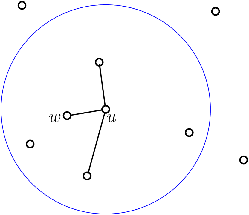
(c) A possible result of the proximity graph construction. Only close pairs are guaranteed to be connected by an edge.

Figure 10: An illustration of the proximity graph construction (Algorithm 1). The blue circle contains $\kappa$ closest nodes to $u$.

References

- [1] N. Alon and J. H. Spencer. The Probabilistic Method. Wiley Publishing, 4th edition, 2016.
- [2] B. Aronov and M. J. Katz. Batched point location in SINR diagrams via algebraic tools. In Automata, Languages, and Programming - 42nd International Colloquium, ICALP 2015, Kyoto, Japan, July 6-10, 2015, Proceedings, Part I, pages 65–77, 2015.
- [3] R. Bar-Yehuda, O. Goldreich, and A. Itai. On the time-complexity of broadcast in multi-hop radio networks: An exponential gap between determinism and randomization. J. Comput. Syst. Sci., 45(1):104–126, 1992.
- [4] L. Barenboim and D. Peleg. Nearly optimal local broadcasting in the SINR model with feedback. In Structural Information and Communication Complexity - 22nd International Colloquium, SIROCCO 2015, Montserrat, Spain, July 14-16, 2015, Post-Proceedings, pages 164–178, 2015.
- [5] B. S. Chlebus, L. Gasieniec, A. Gibbons, A. Pelc, and W. Rytter. Deterministic broadcasting in unknown radio networks. In Proceedings of the Eleventh Annual ACM-SIAM Symposium on Discrete Algorithms, January 9-11, 2000, San Francisco, CA, USA., pages 861–870, 2000.
- [6] A. E. F. Clementi, A. Monti, and R. Silvestri. Selective families, superimposed codes, and broadcasting on unknown radio networks. In S. R. Kosaraju, editor, SODA, pages 709–718. ACM/SIAM, 2001.
- [7] A. E. F. Clementi, A. Monti, and R. Silvestri. Distributed broadcast in radio networks of unknown topology. Theor. Comput. Sci., 302(1-3):337–364, 2003.
- [8] A. Cornejo and F. Kuhn. Deploying wireless networks with beeps. In Distributed Computing, 24th International Symposium, DISC 2010, Cambridge, MA, USA, September 13-15, 2010. Proceedings, pages 148–162, 2010.
- [9] A. Czumaj and W. Rytter. Broadcasting algorithms in radio networks with unknown topology. In FOCS, pages 492–501. IEEE Computer Society, 2003.
- [10] S. Daum, S. Gilbert, F. Kuhn, and C. C. Newport. Broadcast in the ad hoc SINR model. In Y. Afek, editor, Distributed Computing - 27th International Symposium, DISC 2013, Jerusalem, Israel, October 14-18, 2013. Proceedings, volume 8205 of Lecture Notes in Computer Science, pages 358–372. Springer, 2013.
- [11] G. DeMarco. Distributed broadcast in unknown radio networks. SIAM J. Comput., 39(6):2162–2175, 2010.
- [12] Y. Emek, L. Gasieniec, E. Kantor, A. Pelc, D. Peleg, and C. Su. Broadcasting in udg radio networks with unknown topology. Distributed Computing, 21(5):331–351, 2009.
- [13] Y. Emek, E. Kantor, and D. Peleg. On the effect of the deployment setting on broadcasting in euclidean radio networks. Distributed Computing, 29(6):409–434, 2016.
- [14] K. Förster, J. Seidel, and R. Wattenhofer. Deterministic leader election in multi-hop beeping networks - (extended abstract). In Distributed Computing - 28th International Symposium, DISC 2014, Austin, TX, USA, October 12-15, 2014. Proceedings, pages 212–226, 2014.
- [15] F. Fuchs and D. Wagner. On local broadcasting schedules and CONGEST algorithms in the SINR model. In Algorithms for Sensor Systems - 9th International Symposium on Algorithms and Experiments for Sensor Systems, Wireless Networks and Distributed Robotics, ALGOSENSORS 2013, Sophia Antipolis, France, September 5-6, 2013, Revised Selected Papers, pages 170–184, 2013.
- [16] O. Goussevskaia, T. Moscibroda, and R. Wattenhofer. Local broadcasting in the physical interference model. In M. Segal and A. Kesselman, editors, DIALM-POMC, pages 35–44. ACM, 2008.
- [17] H. Gudmundsdottir, E. I. Ásgeirsson, M. H. L. Bodlaender, J. T. Foley, M. M. Halldórsson, and Y. Vigfusson. Extending wireless algorithm design to arbitrary environments via metricity. In 17th ACM International Conference on Modeling, Analysis and Simulation of Wireless and Mobile Systems, MSWiM’14, Montreal, QC, Canada, September 21-26, 2014, pages 275–284, 2014.
- [18] M. M. Halldórsson, S. Holzer, and N. A. Lynch. A local broadcast layer for the SINR network model. In Proceedings of the 2015 ACM Symposium on Principles of Distributed Computing, PODC 2015, Donostia-San Sebastián, Spain, July 21 - 23, 2015, pages 129–138, 2015.
- [19] M. M. Halldórsson and P. Mitra. Towards tight bounds for local broadcasting. In F. Kuhn and C. C. Newport, editors, FOMC, page 2. ACM, 2012.
- [20] M. M. Halldórsson and T. Tonoyan. How well can graphs represent wireless interference? In Proceedings of the Forty-Seventh Annual ACM on Symposium on Theory of Computing, STOC 2015, Portland, OR, USA, June 14-17, 2015, pages 635–644, 2015.
- [21] N. Hobbs, Y. Wang, Q.-S. Hua, D. Yu, and F. C. Lau. Deterministic distributed data aggregation under the sinr model. In Theory and Applications of Models of Computation, pages 385–399. Springer Berlin Heidelberg, 2012.
- [22] T. Jurdzinski and D. R. Kowalski. Distributed backbone structure for algorithms in the sinr model of wireless networks. In M. K. Aguilera, editor, DISC, volume 7611 of Lecture Notes in Computer Science, pages 106–120. Springer, 2012.
- [23] T. Jurdzinski and D. R. Kowalski. Wake-up problem in multi-hop radio networks. In Encyclopedia of Algorithms, pages 2352–2354. Springer, 2016.
- [24] T. Jurdzinski, D. R. Kowalski, M. Rozanski, and G. Stachowiak. Distributed randomized broadcasting in wireless networks under the sinr model. In DISC, pages 373–387, 2013.
- [25] T. Jurdzinski, D. R. Kowalski, M. Rozanski, and G. Stachowiak. On the impact of geometry on ad hoc communication in wireless networks. In M. M. Halldórsson and S. Dolev, editors, ACM Symposium on Principles of Distributed Computing, PODC ’14, Paris, France, July 15-18, 2014, pages 357–366. ACM, 2014.
- [26] T. Jurdzinski, D. R. Kowalski, and G. Stachowiak. Distributed deterministic broadcasting in uniform-power ad hoc wireless networks. In L. Gasieniec and F. Wolter, editors, FCT, volume 8070 of Lecture Notes in Computer Science, pages 195–209. Springer, 2013.
- [27] T. Jurdzinski, M. Rozanski, and G. Stachowiak. Token traversal in ad hoc wireless networks via implicit carrier sensing. SIROCCO 2017, 2017.
- [28] E. Kantor, Z. Lotker, M. Parter, and D. Peleg. The minimum principle of SINR: A useful discretization tool for wireless communication. In IEEE 56th Annual Symposium on Foundations of Computer Science, FOCS 2015, Berkeley, CA, USA, 17-20 October, 2015, pages 330–349, 2015.
- [29] T. Kesselheim. A constant-factor approximation for wireless capacity maximization with power control in the sinr model. In D. Randall, editor, SODA, pages 1549–1559. SIAM, 2011.
- [30] D. R. Kowalski and A. Pelc. Broadcasting in undirected ad hoc radio networks. In Proceedings of the Twenty-second Annual Symposium on Principles of Distributed Computing, PODC ’03, pages 73–82, New York, NY, USA, 2003. ACM.
- [31] A. Ogierman, A. W. Richa, C. Scheideler, S. Schmid, and J. Zhang. Competitive MAC under adversarial SINR. In 2014 IEEE Conference on Computer Communications, INFOCOM 2014, Toronto, Canada, April 27 - May 2, 2014, pages 2751–2759, 2014.
- [32] E. Porat and A. Rothschild. Explicit nonadaptive combinatorial group testing schemes. IEEE Transactions on Information Theory, 57(12):7982–7989, 2011.
- [33] A. W. Richa and C. Scheideler. Jamming-resistant MAC protocols for wireless networks. In Encyclopedia of Algorithms, pages 999–1002. Springer, 2016.
- [34] J. Schneider and R. Wattenhofer. A log-star distributed maximal independent set algorithm for growth-bounded graphs. In Proceedings of the Twenty-Seventh Annual ACM Symposium on Principles of Distributed Computing, PODC 2008, Toronto, Canada, August 18-21, 2008, pages 35–44, 2008.
- [35] D. Yu, Q. Hua, Y. Wang, and F. C. M. Lau. An o(log n) distributed approximation algorithm for local broadcasting in unstructured wireless networks. In IEEE 8th International Conference on Distributed Computing in Sensor Systems, DCOSS 2012, Hangzhou, China, 16-18 May, 2012, pages 132–139, 2012.