Ultra-compact structure in intermediate-luminosity radio quasars: building a sample of standard cosmological rulers and improving the dark energy constraints up to $z\sim 3$

Abstract

In this paper, we present a new compiled milliarcsecond compact radio data set of 120 intermediate-luminosity quasars in the redshift range $0.46<z<2.76$. These quasars show negligible dependence on redshifts and intrinsic luminosity, and thus represents, in the standard model of cosmology, a fixed comoving-length of standard ruler. We implement a new cosmology-independent technique to calibrate the linear size of of this standard ruler as $l_{m}=11.03\pm 0.25$ pc, which is the typical radius at which AGN jets become opaque at the observed frequency $\nu\sim 2$ GHz. In the framework of flat $\Lambda$CDM model, we find a high value of the matter density parameter, $\Omega_{m}=0.322^{+0.244}_{-0.141}$, and a low value of the Hubble constant, $H_{0}=67.6^{+7.8}_{-7.4}\;\rm{kms}^{-1}\rm{Mpc}^{-1}$, which is in excellent agreement with the CMB anisotropy measurements by Planck. We obtain ${\Omega_{m}}=0.309^{+0.215}_{-0.151}$, $w=-0.970^{+0.500}_{-1.730}$ at 68.3% CL for the constant $w$ of a dynamical dark-energy model, which demonstrates no significant deviation from the concordance $\Lambda$CDM model. Consistent fitting results are also obtained for other cosmological models explaining the cosmic acceleration, like Ricci dark energy (RDE) or Dvali-Gabadadze-Porrati (DGP) brane-world scenario. While no significant change in $w$ with redshift is detected, there is still considerable room for evolution in $w$ and the transition redshift at which $w$ departing from -1 is located at $z\sim 2.0$. Our results demonstrate that the method extensively investigated in our work on observational radio quasar data can be used to effectively derive cosmological information. Finally, we find the combination of high-redshift quasars and low-redshift clusters may provide an important source of angular diameter distances, considering the redshift coverage of these two astrophysical probes.

1 Introduction

That the expansion of the Universe is accelerating at the current epoch has been demonstrated by the observations of Type Ia supernovae (SN Ia) (Riess et al., 1998; Perlmutter et al., 1999) and also supported by other independent probes, such as the Cosmic Microwave Background (CMB) (Pope et al., 2004) and the Large Scale Structure (LSS) (Spergel et al., 2003). Therefore, the so called dark energy (DE), a new component driving the observed accelerated expansion of the Universe was introduced into the framework of general relativity. However, the nature of this exotic source with negative pressure has remained an enigma.

Besides the cosmological constant $\Lambda$ (Peebles & Ratra, 2003), the simplest candidate consistent with current observations, which however suffers from the well-known fine tuning and coincidence problems, other possible dark energy models with different dark energy equation of state (EoS) parametrizations (Ratra et al., 1988; Chevalier & Polarski, 2001; Linder, 2004) have also been the focus of investigations in recent decades. Meanwhile, it should be noted that cosmic acceleration might also be explained by possible departures of the true theory of gravity from General Relativity. From these theoretical motivations, possible multidimensionality in the brane theory gave birth to the well-known Dvali-Gabadadze-Porrati (DGP) model, while the holographic principle has generated the Ricci dark energy (RDE) model. All above mentioned models are in agreement with some sets of observational data, e.g. the distance modulus from SNIa, or the CMB anisotropies. At this point, it is worth to highlight the issue of evolving the equation of state $w(z)$ of dark energy. Namely, a dynamical DE will be indicated by $w(z)$ evolving across -1, rather than having a fixed value $w(z)=-1$, which implies an additional intrinsic degree of freedom of dark energy, and could be a smoking gun of the breakdown of Einstein’s theory of general relativity on cosmological scales (Zhao et al., 2012). However, due to the so-called “redshift desert” , it is very difficult to check dynamical DE from astrophysical observations. When confronted with such theoretical and observational puzzles, we have no alterative but turn to high-precision data and develop new complementary cosmological probes at higher redshifts. In this paper we propose that compact structure measurements in radio quasars leading to calibrated standard rulers can become a useful tool for differentiating between the above mentioned dark energy models and exploring possible dynamical evolution of $w(z)$.

In the framework of standard cosmology, over the past decades considerable advances have been made in the search for possible candidates to serve as “true” standard rods in the Universe. In particular, cosmological tests based on the angular size — distance relation have been developed in a series of papers, and implemented using various astrophysical sources. Recently, attention of has been focused on large comoving length scales revealed in the baryon acoustic oscillations (BAO). The BAO peak location is commonly recognized as a fixed comoving ruler of about $105h^{-1}\;Mpc$ (where $h$ is the Hubble constant $H_{0}$ expressed in units of $100\;km\,s^{-1}Mpc^{-1}$). However, the so-called fitting problem (Ellis & Stoeger, 1987) still remains a challenge for BAO peak location as a standard ruler. In particular, the environmental dependence of the BAO location has recently been detected by Roukema et al. (2015, 2016). Moreover, Ding et al. (2015) and Zheng et al. (2016) pointed out a noticeable systematic difference between $H(z)$ measurements based on BAO and those obtained with differential aging techniques. Much efforts have also been made to explore the sizes of galaxy clusters at different redshifts, by using radio observations of the Sunyaev-Zeldovich effect together with X-ray emission (De Filippis et al., 2005; Bonamente et al., 2006). However, the large observational uncertainties of these angular diameter distance measurements significantly affect the constraining power of this standard ruler. Actually, clusters alone could not provide a competitive source of angular diameter distance to probe the acceleration of the Universe.

In the similar spirit, radio sources constitute a specially powerful population to test the redshift - angular size relation for extended FRIIb galaxies (Daly & Djorgovski, 2003), radio galaxies (Guerra & Daly, 1998; Guerra, Daly & Wan, 2000), and radio loud quasars (Buchalter et al., 1998). For instance, it was firstly proposed that the canonical maximum lobe size of radio galaxies may provide a standard ruler for cosmological studies. From the mean observed separation of a sample of 14 radio lobes, in combination with the measurements of radio lobe width, lobe propagation velocity, and inferred magnetic field strength, Guerra & Daly (1998) found $\Omega_{m}=0.2^{+0.3}_{-0.2}$ (68% confidence) for a flat cosmology.

More promising candidates in this context are ultra-compact structure in radio sources (especially for quasars that can be observed up to very high redshifts), with milliarcsecond angular sizes measured by very-long-baseline interferometry (VLBI) (Kellermann, 1993; Gurvits, 1994). For each source, the angular size is defined as the separation between the core (the strongest component) and the most distant component with 2% of the core peak brightness (Kellermann, 1993). The original data set compiled by Gurvits, Kellerman & Frey (1999) comprises 330 milliarcsecond radio sources covering a wide range of redshifts and includes various optical counterparts, such as quasars and radio galaxies (hereafter we call this data G99 for short). After excluding sources with synthesized beam along the direction of apparent extension, compact sources unresolved in the observed VLBI images were naturally obtained. Finally, in order to minimize possible dependence of angular size on spectral index and luminosity, the final sample was restricted to 145 compact sources with spectral index ($-0.38\leq\alpha\leq 0.18$) and total luminosity ($Lh^{2}\geq 10^{26}\;WHz^{-1}$). Possible cosmological application of these compact radio sources as a standard rod has been extensively discussed in the literature (Vishwakarma, 2001; Zhu & Fujimoto, 2002; Chen & Ratra, 2003). In their analysis, the full data set of 145 sources was distributed into twelve redshift bins with about the same number of sources per bin. The lowest and highest redshift bins were centered at redshifts $z=0.52$ and $z=3.6$ respectively. However, the typical value of the characteristic linear size $l_{m}$ remained one of the major uncertainties in their analysis. In order to provide tighter cosmological constraints, some authors chose to fix $l$ at specific values (Vishwakarma, 2001; Lima & Alcaniz, 2002; Zhu & Fujimoto, 2002), while Chen & Ratra (2003) chose to include a large range of value for $l$ and then integrate it over to obtain the probability distribution of parameters of interest.

The controversy around the exact value of the characteristic linear size $l_{m}$ for this standard rod or even whether compact radio sources are indeed “true” standard rods still existed. Under the assumption of a homogeneous, isotropic universe without cosmological constant, Gurvits, Kellerman & Frey (1999) and Vishwakarma (2001) suggested that the exclusion of sources with extreme spectral indices and low luminosities might alleviate the dependence of $l_{m}$ on the source luminosity and redshift. More recently, Cao et al. (2015a) reexamined the same data in the framework of $\Lambda$CDM cosmological model, and demonstrated that both source redshift and luminosity will affect the determination of the radio source size, i.e. the mixed population of radio sources including different optical counterparts (quasars, radio galaxies, etc.) cannot be treated as a “true” standard rod. In their most recent work, however, by applying the popular parametrization $l_{m}=lL^{\beta}(1+z)^{n}$, Cao et al. (2017a) found that, compact structure in the intermediate-luminosity radio quasars could serve as a standard cosmological rod minimizing the above two effects ($|n|\simeq 10^{-3}$, $|\beta|\simeq 10^{-4}$), and thus provide valuable sources of angular diameter distances at high reshifts ($z\sim 3.0$), reaching beyond feasible limits of supernova studies. On the other hand, through the investigation of the calibrated value for $l_{m}$, we will focus on the astrophysical implication of the linear size for this standard ruler. As we “look” into the jet of AGN, the plasma is initially optically thin (transparent), but gets less as we look further in and the plasma density increases; eventually the plasma becomes optically thick (opaque), which point we identify with the “core”.

The focus of this paper is on two issues. First, we extend recent analysis Cao et al. (2017a) of compact sources as standard rulers. The extension is related to completely cosmological-model independent calibration of the linear size of standard rulers. This was not possible in previous study where the speed of light was discussed. Then, the angular size measurements of 120 quasars covering redshift range $z=0.46-2.76$ will be used to constrain dynamical properties of dark energy in a way competitive with other probes and reaching to higher redshifts than other distance indicators. This way we will demonstrate the usefulness of the sample presented. The outline of the paper is as follows: in Section 2 we briefly describe the quasar data and a cosmological model independent method of calibrating the linear size of this standard ruler. In Section 3 we report the results of constraints on the properties of dark energy obtained with the quasar data. Section 4 is devoted to constraints on other mechanisms explaining the cosmic acceleration. Finally, we give our discussion and conclusions in Section 5 and 6, respectively.

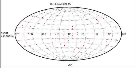
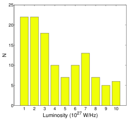
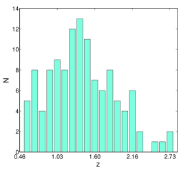
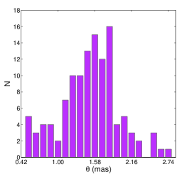
Figure 1: Upper: Sky distribution of the quasar sample of 120 sources detected with VLBI. Lower: Luminosity, redshift, and angular size distribution for the quasar sample of 120 sources.

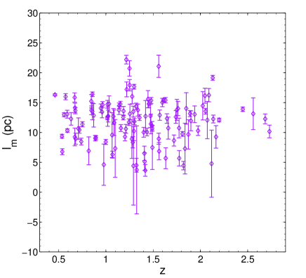
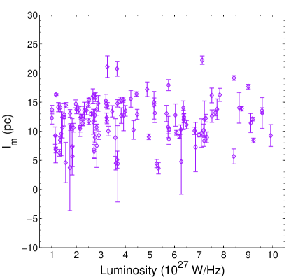
Figure 2: The intrinsic metric linear size $l_{m}$ distribution of the 120 intermediate luminosity quasars in the redshift and luminosity space.

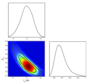
Figure 3: Degeneracy between the linear size of ultra-compact structure in radio quasars and the matter density parameter in the Universe; $68.3\%$ and $95.4\%$ confidence regions are shown.

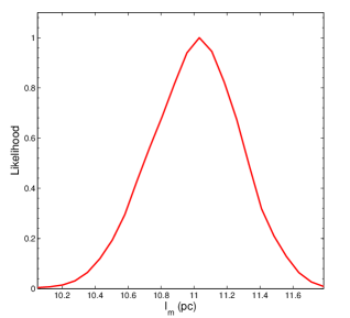
Figure 4: The corrected linear size of compact quasars derived in a cosmological model independent way, using the observational $H(z)$ data.

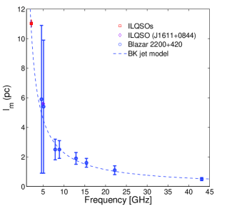
Figure 5: The plot of core size versus frequency (Constraint on the linear size of compact structure in intermediate-luminosity quasars $l$ at 2.16 GHz is added). BK 79 jet model ($r_{c}\propto\nu^{-1}$ )is used for the fitted curve from VLBI/VLBA observations in the literature.

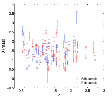
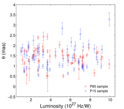
Figure 6: Comparison between P15 and P85 samples concerning the “angular size - redshift” and “angular size - luminosity” diagrams based on 58 sources common to these two surveys.

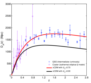
Figure 7: The angular diameter distances $D_{A}(z)$ estimated from quasars as standard rulers (blue squares). Angular diameter distances from galaxy clusters (purple circles) are also added for comparison. Theoretical predictions of $\Lambda$CDM models with $\Omega_{\Lambda}=0.00$ and $\Omega_{\Lambda}=0.70$ are denoted by black and red solid lines, respectively.

2 Data and method

The data to be used here are derived from a compilation of angular-size/redshift data for ultra-compact radio sources, from an ancient VLBI survey undertaken by Preston et al. (1985) (hereafter we call this data P85 for short). By employing a world-wide array of dishes forming an interferometric system with an effective baseline of about $8\times 10^{7}$ wavelengths, this survey succeeded to detect 917 sources with compact structure out of 1398 known radio sources. The results of this survey were utilized initially to provide a very accurate VLBI celestial reference frame, improving precision by at least an order of magnitude, compared with earlier stellar frames. An additional expectation was that the catalog would be “used in statistical studies of radio-source properties and cosmological models” (Preston et al., 1985). By considering a sample including 258 objects with redshifts $z>0.5$, the possibility of applying this sample to cosmological study was firstly proposed by Gurvits (1994) and then extended by Jackson & Dodgson (1997); Jackson (2004); Jackson & Jannetta (2006); Cao et al. (2017a). We will use a revised sample comprising 613 objects with reshifts $0.0035\leq z\leq 3.787$, which sample is a recent upgrade with regard to redshift based on P85 (Jackson & Jannetta, 2006) .

All detected sources included in this comprehensive compilation were imaged with VLBI at 2.29 GHz, which involve a wide class of extragalactic objects including quasars, radio galaxies, BL Lac objects (blazars), etc. It should be noted that P85 does not give contour maps, and does not list angular sizes explicitly; however, total flux density and correlated flux density (fringe amplitude) are listed; the ratio of these two quantities is the visibility modulus $\Gamma$, which defines a characteristic angular size

$$\theta={2\sqrt{-\ln\Gamma\ln 2}\over\pi B}$$ (1)

where $B$ is the interferometer baseline, measured in wavelengths (Thompson, Moran & Swenson, 1986, p. 13; Gurvits, 1994). The angular sizes used here were calculated using equation (1); it is argued in Jackson (2004) that this size represents that of the core, rather than the angular distance between the latter and a distant weak component.

In our analysis, by applying two selection criteria, one on spectral index ($-0.38\leq\alpha\leq 0.18$) and the second on luminosity ($10^{27}$ W/Hz$<L<$$10^{28}$ W/Hz), we will focus our attention on the compact structure in 120 radio quasars with flat spectral index and intermediate luminosity. Recent study of Cao et al. (2017a) suggested that they can be effectively used as standard rulers. Full information about the said 120 sources can be found in Table 1, including source coordinates, redshifts, angular size, spectral index, and total flux density. The corresponding optical counterpart for each system can be found in P85. Fig. 1 is an equal-area sky-distribution plot of the detected quasars. The distribution of redshifts, luminosities, and angular-sizes of the sources in our sample is also shown in Fig. 1, which simply reflects the fact that our basically luminosity-limited sample, compiled on an ad-hoc basis from the literature and based upon various selection criteria, is relatively homogenous both in redshifts and angular-sizes. The angular sizes of the sample range from 0.424 to 2.743 milliarcsec, with 15% of the quasars having angular sizes $\theta<1$ mas, and only a handful of quasars with larger angular sizes ($\theta>2$ mas) have been identified, while 75% of all quasars are located at 1.0 mas$<\theta<2.0$ mas. We remark here that, the final sample covers the redshift range $0.46<z<2.76$, which indicates its potential usefulness in cosmology at high redshifts.

For a cosmological rod with intrinsic length $l_{m}$, the angular size-redshift relation can be written as (Sandage, 1988)

$$\theta(z)=\frac{l_{m}}{D_{A}(z)}$$ (2)

where $\theta(z)$ is the angular size at redshift $z$, and $D_{A}(z)$ is the corresponding angular diameter distance. $D_{A}(z)$ is related to $H_{0}$, the Hubble constant, and $E(z;\textbf{p})$, the dimensionless expansion rate depending on redshift $z$ and cosmological parameters p. However, the cosmological application of such technique requires good knowledge of the linear size of the “standard rod” used. The possibility that source’s linear size depends on the source luminosity and redshift should be kept in mind. In this analysis, we use a phenomenological model to characterize the relations between the projected linear size of a source and its luminosity $L$ and redshift $z$ (Gurvits, 1994; Gurvits, Kellerman & Frey, 1999; Cao et al., 2017a)

$$l_{m}=lL^{\beta}(1+z)^{n}\,$$ (3)

where $l$ is the linear size scaling factor, $\beta$ and $n$ quantify the dependence of the linear size on source luminosity and redshift, respectively (Gurvits, 1994). Following the analysis of Cao et al. (2017a), for our quasar sample, the linear size $l_{m}$ is independent of both redshift and luminosity ($|n|\simeq 10^{-3}$, $|\beta|\simeq 10^{-4}$) and there is only one parameter $l$ to be considered. The intrinsic metric linear size $l_{m}$ distribution of the 120 intermediate luminosity quasars in the redshift and luminosity space is shown in Fig. 2. Since both the $l_{m}$ (calculated from Eq. 2) and luminosity require the knowledge of angular diameter distances, we used $D_{A}(z)$ values at the quasars’ redshifts inferred from the Hubble parameter ($H(z)$) measurements, i.e. in a cosmological model independent way (see Cao et al. (2017a) for details). The measurements of $H(z)$ are acquired by means of two different techniques: one is called cosmic chronometers (Jimenez & Loeb, 2002), i.e. massive, early-type galaxies evolving passively on a timescale longer than their age difference, while the other comes from the analysis of baryon acoustic oscillations (BAO). One can see from Fig. 2 that intermediate-luminosity quasars could serve as standard rulers, much better than other quasar sub-samples discussed in Cao et al. (2017a). Therefore, if we could find a suitable method to calibrate $l$, then we would get stringent constraints on the angular diameter distances at different redshifs, and thus relevant cosmological parameters p. In order to check the degeneracy between p and $l$, we investigated our radio quasar sample in the framework of the concordance $\Lambda$CDM cosmology, which is characterized by two free parameters, the matter density $\Omega_{m}$ and the intrinsic linear size $l$. Fig. 3 shows the corresponding confidence regions.

Now a cosmological-model-independent method will be applied to derive the linear size of the compact structure in intermediate-luminosity radio quasars. Namely, cosmic chronometer $H(z)$ measurements processed using Gaussian Processes (GP) (Li et al., 2016) can provide us angular diameter distances $D_{A}$ covering the quasar redshift range, and thus allows us to calibrate the angular size of milliarcsecond quasars. In the so-called cosmic chronometers (Jimenez & Loeb, 2002), the cosmic expansion rates $H(z)$ are measured from age estimates of red galaxies without any prior assumption of cosmology, i.e., $H(z)\simeq-\frac{1}{1+z}\frac{\Delta z}{\Delta t}$. In order to minimize the systematic effects, we used the $H(z)$ sample following the choice of Moresco et al. (2012); Verde et al. (2014); Li et al. (2016). Currently, based on this method, 30 measurements of $H(z)$ covering the redshift range $0.070\leq z\leq 1.965$ have been obtained. See Zheng et al. (2016) for details and reference to the source papers. However, according to the analysis of Moresco et al. (2012), the choice of stellar population synthesis model may strongly affect these estimates of $\Delta t$ and thus $H(z)$, especially at $z\geq 1.2$. Therefore, we consider only 24 $H(z)$ measurements up to $z<1.2$ in this paper. Moreover, following the analysis of Verde et al. (2014); Li et al. (2014), the error bar of the highest-$z$ point is increased by 20% to include the uncertainties of the stellar population synthesis models.

According to Holanda et al. (2013), for a non-uniformly distributed $H(z)$ data, the comoving distance integral could be obtained with a simple trapezoidal rule

$$D(z)=c\int_{0}^{z}\frac{dz^{\prime}}{H(z^{\prime})}\approx\frac{c}{2}\sum_{i=1}^{N}(z_{i+1}-z_{i})\bigg{(}\frac{1}{H_{i+1}}+\frac{1}{H_{i}}\bigg{)}.$$ (4)

Concerning the fact that the number of data points and the uniformity of the spaced data will heavily influence the precision of this simple rule, we will use Gaussian Processes (GP), a powerful non-linear interpolating tool to reconstruct the evolution of the expansion rate with redshift, and thus integrate its inverse function to estimate distances in a cosmological model-independent way (Holanda et al., 2013). This method was firstly proposed to test both cosmology (Holsclaw et al., 2010a, b) and cosmography (Shafieloo et al., 2013), and then extensively applied to the derivation of the Hubble constant $H_{0}$ (Busti et al., 2014), the reconstructions of the equation of state of dark energy (Seikel et al., 2013) and the distance-duality relation (Zhang, 2014). The advantage of Gaussian processes is, that we do not need to assume any parametrized model for $H(z)$ while reconstructing this function from the data (Holsclaw et al., 2010a, b). Moreover, with a very small and uniform step of $\Delta z=z_{i+1}-z_{i}$, we may obtain more precise measurements of angular diameter distances at a certain redshift. In order to reconstruct the Hubble parameter as a function of the redshift from 24 $H(z)$ measurements of cosmic chronometers covering $z=(0.0,1.2)$ we used the publicly available code (Seikel et al., 2013) called the GaPP (Gaussian Processes in Python) .

Applying the redshift-selection criteria, $\Delta z=|z_{QSO}-z_{H}|\leq 0.005$ to the angular diameter distances derived from $H(z)$, we obtain 48 measurements of $D_{A}$ coinciding with the quasars reshifts. Undertaking similar analysis as Cao et al. (2017a), we obtain constraints on the linear size $l_{m}$ with the best fit

$$l_{m}=11.03\pm 0.25\ \mathrm{pc}.$$ (5)

The probability distribution of $l_{m}$ is also shown in Fig. 4, which will be used in the following cosmological analysis with quasar observations. Note, that in our previous paper (Cao et al., 2017a) which aimed at estimation of the velocity of light with extragalactic sources, such calibration was not be possible because of the appearance of $c$ in the expression for $D_{A}$ (see e.g. Eq. 4). Two issues deserve attention. First is that the rigid assumption of vanishing $\beta$ and $n$ parameters describing evolution of the comoving size $l_{m}$ with luminosity and redshift might introduce a bias and underestimate the uncertainties of cosmological parameters fitted. Second is whether the cosmic chronometers used for calibrating QSO as standard rulers introduce a bias. These points will be addressed in the following sections by modelling $\beta$ and $n$ parameters with Gaussian distributions and by comparison of the results obtained with quasars as standard rulers and with $H(z)$ data alone.

Now we try to make some comments on the physical meaning of the linear size of this standard ruler. For a long time it has been argued that Active Galactic Nuclei (AGN) must be powered by accretion of mass onto massive black holes. Current theoretical models indicate that jets of relativistic plasma are generated in the central regions of AGN, and magnetic fields surrounding the black hole expel, accelerate and help to collimate the jet flow outwards (Meier, 2009). According to the unified classification of Active Galactic Nuclei (AGN), 10 pc is the typical radius at which AGN jets are apparently generated and there is almost no stellar contribution (Blandford & Rees, 1978). In the conical jet model proposed by Blandford & Königl (1979) [hereafter BK79], with the base of the jet corresponding to the vertex of the cone, the unresolved core is identified with the innermost, optically thick region of the approaching jet. For QSOs, this compact opaque parsec-scale core is located between the broad-line region ($\sim$ 1 pc) and narrow-line region ($\sim$ 100 pc) (Blandford & Rees, 1978).

More recently, Hopkins & Quataert (2010) have investigated the correlation between the black hole’s mass accretion rate $\dot{M}_{BH}$ and the star-formation rate $\dot{M}_{\ast}$. Their results from simulations showed that, within the central 10 pc around the black hole, the star formation rate is equal to the mass accretion rate. This conclusion is well-consistent with the recent observations by Silverman et al. (2009). Frey et al. (2010) has presented high-resolution radio structure imaging of five quasars (J0813+3508, J1146+4037, J1242+5422, J1611+0844, and J1659+2101) at $4.5<z<5$ with the European VLBI Network (EVN) at 5 GHz. Although all cases have satisfied the intermediate-luminosity criterion defined in this paper, there is only one flat-spectrum source (J1611+0844) which could be used for comparison in our analysis, while the compact emission of other quasars is characterized by a steep radio spectrum (Frey et al., 2010). Moreover, we combine our constraint with the recent observation of Blazar 2200+420 from the Very Long Baseline Array (VLBA), at eight frequencies (4.6, 5.1, 7.9, 8.9, 12.9, 15.4, 22.2, 43.1 GHz), to investigate the frequency-dependent position of VLBI cores . From the comparison presented in Fig. 5 and Table 2, we find a very good consistency between the measurements and the BK79 conical jet model, in which the position of the radio core follows $r\propto\nu^{-1}$, where $r$ is the distance from the central engine (Blandford & Königl, 1979), if the core is self-absorbed and in equipartition. As noted in the analysis of Cao et al. (2017a), our estimate of $l_{m}$ is also well consistent with the results derived from recent multi-frequency VLBI imaging observations of more than 3000 compact extragalactic radio sources (Pushkarev & Kovalev, 2015). In fact, 58 intermediate-luminosity quasars included in our modified P85 sub-sample have also been observed by recent VLBI observations based on better uv-coverage in the P15 sample. Based on these 58 sources, one may compare P15 and P85 samples on the “angular size - redshift” and “angular size - luminosity” diagrams. This is displayed in Fig. 6, from which one can see some difference between the samples concerning estimates of the angular size. However, we checked that the characteristic linear size $l_{m}$ at 2 GHz estimated from P15 is well-consistent with the results obtained from the P85 sample. Astrophysical application of the recent multi-frequency angular size measurements of 58 intermediate-luminosity quasars from the P15 sample, will be subject of the next work in preparation (Cao et al., 2017b).

If one, quite straightforwardly, attempts to construct an empirical relation $D_{A}(z)$ extending to higher redshifts on the basis of individual quasar angular sizes, using Eq. (2), one can obtain the $D_{A}$ measurement and the corresponding uncertainty for each quasar. However, this procedure results in large uncertainties in $D_{A}$, which problem has been encountered previously (Gurvits, 1994; Gurvits, Kellerman & Frey, 1999), as can be seen from plots of the measured angular size against redshift therein. This problem remains even after 13 systems with very large ($\sim 50\%$) uncertainties are removed. Therefore, in order to minimize its influence on our analysis, we have chosen to bin the remaining 107 data points and to examine the change in $D_{A}$ with redshift. The final sample was grouped into 20 redshift bins of width $\Delta z=0.10$. Fig. 7 shows the median values of $D_{A}$ for each bin plotted against the central redshift of the bin. For comparison, the two curves plotted as solid lines represent theoretical expectations from the concordance $\Lambda$CDM model and the Einstein - de Sitter model. One can see that the latter is disfavored at high confidence. More importantly, the angular diameter distance information obtained from quasars has helped us to bridge the “redshift desert” and extend our investigation of dark energy to much higher redshifts. It is worth noting that these 120 intermediate-luminosity QSOs are obtained in a completely cosmology-independent method, and hence can be used to constrain cosmological parameters without the circularity problems.

3 Constraints on dark energy

In this section, we investigate some dark energy models and estimate their best-fitted parameters using the quasar sample. Models discussed in this section are aimed at explaining the accelerated expansion of the universe by introducing a hypothetical fluid whose contribution to the matter budget and equation of state are unknown parameters to be fitted. Next section 4, will discuss alternative concepts involving departure from classical General Relativity. More specifically, the following models for dark energy will be studied in this section:

• $\Lambda$CDM: cosmological constant in a flat universe.

• XCDM: constant equation-of-state parameter in a flat universe.

• $w_{z}$CDM: time-varying equation-of-state parameter in a flat universe.

We determine the cosmological model parameters p using a $\chi^{2}$ minimization method.

$$\chi^{2}(\textbf{p})=\sum_{i}^{120}{\frac{\left[\theta(z_{i};l_{m};\textbf{p})-\theta_{oi}\right]^{2}}{\sigma_{i}^{2}}},$$ (6)

where $\theta(z_{i};\textbf{p})=l_{m}/D_{A}$ is the angle subtended by an object of proper length $l_{m}$ transverse to the line of sight and $\theta_{oi}$ is the observed value of the angular size with uncertainties $\sigma_{i}$. The summation is over all the 120 observational data points. In computing $\chi^{2}$ we have also assumed additional 10% uncertainties in the observed angular sizes, to account for both observational errors and the intrinsic spread in linear sizes. We remark here that, although the best-fit values of $\beta$ and $n$ parameters, describing the dependence of $l_{m}$ on the luminosity and redshift, are negligibly small, yet their uncertainties could also be an important source of systematic errors on the final cosmological results. In order to address this issue, we perform a sensitivity analysis by applying Monte Carlo simulations in which $\beta$, $n$ were characterized by Gaussian distributions: $\beta=0.00\pm 0.05$ and $n=0.00\pm 0.05$, while the uncertainty of the linear size scaling factor was taken into account with a Gaussian distribution as $l=11.03\pm 0.25$ pc .

In a similar manner as in other papers introducing new compilations of cosmologically important data sets, e.g. Amanullah et al. (2010), we constrain the properties of dark energy first using QSO alone (with and without the systematic uncertainty of $l$, $\beta$ and $n$), and then perform combined analysis using also the latest CMB data from Planck Collaboration XIV (2016), and the BAO data from 6dFGS, SDSS-MGS, BOSS-LOWZ, and BOSS-CMASS (Beutler et al., 2011; Ross et al., 2015; Anderson et al., 2014). Moreover, considering that there is no strong evidence for the departure from spatially flat geometry at the current data level, which is known from and strongly supported by other independent and precise experiments (Planck Collaboration XIII, 2016; Planck Collaboration XIV, 2016), we will assume spatial flatness of the Universe throughout the following analysis in the paper. The results for each of the models are listed in Table 2 and discussed in turn in the following sub-sections. Unless stated otherwise, the uncertainties represent the 68.3% confidence limits and include both statistical uncertainties and systematic errors. In addition, we add the prior for the Hubble constant $H_{0}=67.3\;\rm{kms}^{-1}\rm{Mpc}^{-1}$ after Planck Collaboration XVI (2014). The exceptions are the $\Lambda$CDM and the DGP models (next section) where $H_{0}$ is treated as a free parameter.

3.1 $\Lambda$CDM

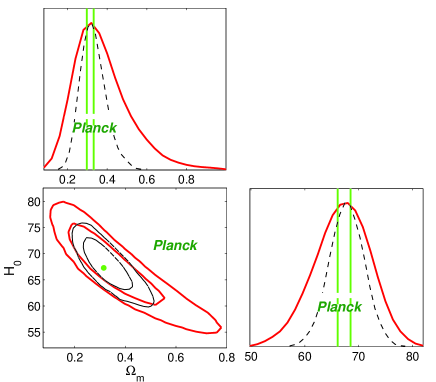
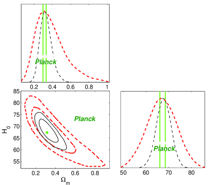
Figure 8: Cosmological constraints on the flat $\Lambda$CDM model from the quasar sample without (left panel) and with systematical uncertainties (right panel). Fitting results from recent $H(z)$ measurements (black dashed lines) and Planck observations (green dot represents the best-fist with $1\sigma$ errors denoted by green solid lines) are also added for comparison.

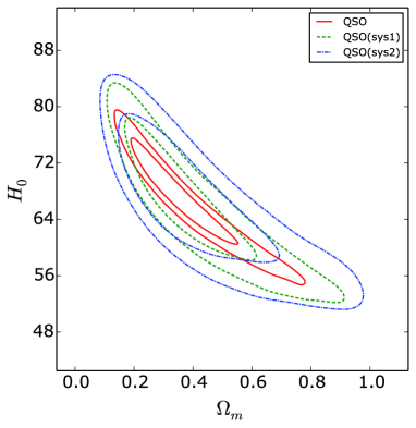
Figure 9: Cosmological constraints on the flat $\Lambda$CDM model from the quasar sample without and with different systematical uncertainties: sys1 denotes the systematics with $l=11.03\pm 0.25$pc, $\beta=0.00\pm 0.05$ and $n=0.00\pm 0.05$, while sys2 represents the systematics with $l=11.03\pm 0.25$pc, $\beta=0.00\pm 0.10$ and $n=0.00\pm 0.10$.

If flatness of the FRW metric is assumed, the only cosmological parameter of this model is ${\bf{p}}=\left\{\Omega_{m}\right\}$. However, in order to check the constraining power of our quasar data on the Hubble constant, we choose to take $H_{0}$ as the other free parameter and obtained $\Omega_{m}=0.322^{+0.244}_{-0.141}$ and $H_{0}=67.6^{+7.8}_{-7.4}\;\rm{kms}^{-1}\rm{Mpc}^{-1}$. After including systematics due to uncertainties on $l$, $\beta$ and $n$, the matter density parameter and Hubble constant respectively change to $\Omega_{m}=0.312^{+0.295}_{-0.154}$ and $H_{0}=67.0^{+11.2}_{-8.6}\;\rm{kms}^{-1}\rm{Mpc}^{-1}$. These results are presented in Fig. 8. Now one issue which should be discussed is how much the cosmological parameters are affected by larger uncertainties of $\beta$ and $n$. For this purpose, we changed the uncertainty of the luminosity-dependence parameter to $\beta=0.00\pm 0.10$ and the redshift-dependence parameter to $n=0.00\pm 0.10$. The comparison of the resulting constraints on $\Omega_{m}$ and $H_{0}$ based on different systematical uncertainties is shown in Fig. 9. One can easily check that reduction of the error of $\beta$ and $n$ will lead to more stringent cosmological fits, which motivates us to improve constraints on the two parameters with a larger quasar sample from future VLBI observations based on better uv-coverage (Pushkarev & Kovalev, 2015).

Another important issue is the comparison of our cosmological results with those of earlier studies done using other, alternative probes. We start by comparing our results with fits obtained using $H(z)$ measurements from cosmic chronometers. Respective likelihood contours obtained with the latest $H(z)$ data comprising 30 data points (Zheng et al., 2016) are also plotted in Fig. 8. We see that 1$\sigma$ confidence regions from these two techniques overlap very well with each other. This means that the results obtained on the sample of quasars are well consistent with the $H(z)$ fits, although with larger uncertainties due to systematic uncertainties of the parameters characterizing this standard ruler. Central fits however, are almost the same. Besides, looking at the constraints obtained with QSO and $H(z)$ data, we find similar degeneracy between $\Omega_{m}$ and $H_{0}$. Moreover, the constraint on $\Omega_{m}$ derived from the mean observed separation of the radio lobes (Daly & Djorgovski, 2003; Guerra & Daly, 1998; Guerra, Daly & Wan, 2000) is in broad agreement with the results we report. Then, gravitational lensing systems with QSO acting as sources may provide us another probe of angular diameter distance data in cosmology, since strong gravitational lensing statistics depends on the angular diameter distances between the source, the lens, and the observer. Using the redshift distribution of radio sources, Chiba & Yoshii (1999) calculated the absolute lensing probability for both optical and radio lenses. The best-fit mass density obtained in their analysis in a flat cosmology, $\Omega_{m}=0.3^{+0.2}_{-0.1}$, is consistent with our results. Constraints on cosmological models using strong lensing statistics have been obtained e.g. in Biesiada, Piórkowska, & Malec (2010); Cao et al. (2012); Cao, Covone & Zhu (2012); Cao et al. (2015b). At last, based on the first-year Planck results, Planck Collaboration XVI (2014) gave the best-fit parameter: ${\Omega_{m}}=0.315\pm 0.017$ and $H_{0}=67.3\pm 1.2\;\rm{kms}^{-1}\;\rm{Mpc}^{-1}$ for the flat $\Lambda$CDM model, which is in perfect agreement with our standard ruler result. In contrast, compared with our quasar sample, recent combined SNLS SNe Ia data favors a lower value of $\Omega_{m}$ and thus smaller matter density in the $\Lambda$CDM model than our quasar data (Conley et al., 2011). Let us note that the cosmological probe inferred from CMB anisotropy measured by Planck is also a standard ruler — the comoving size of the acoustic horizon. Therefore appreciable consistency between the same type of probes (standard rulers) could be expected and indeed is revealed here.

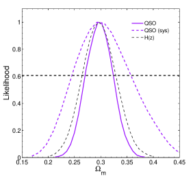
Figure 10: The probability distribution of the matter density parameter in the flat $\Lambda$CDM model, which is derived from the quasar sample without (red solid line) and with systematical uncertainties (red dashed line) with the prior on the Hubble constant $H_{0}=70$ km $\rm s^{-1}$ $\rm Mpc^{-1}$. Fitting result from recent $H(z)$ measurements (black dashed lines) is also added for comparison.

We emphasize that the value of the Hubble constant obtained in our analysis, is in excellent agreement with the findings based on Planck CMB data. Many previous have determined its present value with other probes. For example, the final results of the Hubble Space Telescope (HST) key project suggested the Hubble constant as $H_{0}=72\pm 8\;\rm{kms}^{-1}\rm{Mpc}^{-1}$ (Freedman et al., 2001). Then, the observations of 240 HST Galactic Cepheid variables gave $H_{0}=74.2\pm 3.6\;\rm{kms}^{-1}\rm{Mpc}^{-1}$ (Riess et al., 2009). Much lower value has been suggested by Tammann et al. (2008) who independently calibrated Cepheids and SN Ia and obtained $H_{0}=62.3\pm 1.3\;\rm{kms}^{-1}\rm{Mpc}^{-1}$. Two most recent measurements of the Hubble constant are $H_{0}=69.6\pm 0.7$ km $\rm s^{-1}$ $\rm Mpc^{-1}$ (Bennett et al., 2014) and that obtained from local Cepheids distance ladder, $H_{0}=73.24\pm 1.74\;\rm{kms}^{-1}\rm{Mpc}^{-1}$ (Riess et al., 2016). It is also worth noticing that, according to the meta-analysis of existing literature based on median statistics (Gott et al., 2001; Chen & Ratra, 2003) the value of $H_{0}=68\;\rm{kms}^{-1}\;\rm{Mpc}^{-1}$ can be considered as the most likely value for the Hubble constant. In order to check the cosmological constraint power of the quasar sample derived in this analysis, we set the $H_{0}=70$ km $\rm s^{-1}$ $\rm Mpc^{-1}$ prior and obtain a very stringent fit on the the present-day matter density $\Omega_{m}=0.297\pm 0.027$ (without systematics) and $\Omega_{m}=0.300\pm 0.055$ (with systematics). This is shown in Fig. 10. For comparison, fitting result from the $H(z)$ data is also plotted with black dashed line. It is obvious that the current quasar observations could provide consistent and comparable cosmological constraints with respect to the cosmic chronometers.

3.2 XCDM model

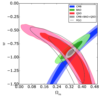
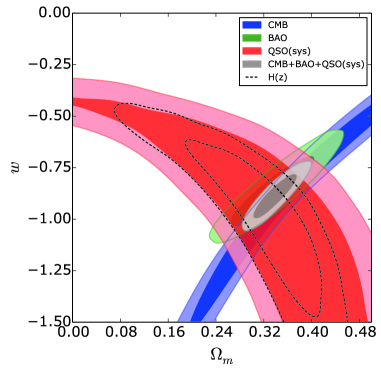
Figure 11: XCDM model: 68.3% and 95.4% confidence regions in the ($\Omega_{m}$, $w$) plane from QSO, BAO, CMB and $H(z)$. The left panel shows the QSO confidence region with the best-fit value for $l$ only, while the right panel shows the confidence region including systematical uncertainties of $l$, $\beta$ and $n$. We note that CMB and QSO constraints are orthogonal, making this combination of cosmological probes very powerful for investigating the nature of dark energy.

Allowing for a deviation from the simple $w=-1$ case, an alternative is dynamical energy based exclusively on a scalar field (Ratra et al., 1988). In this case, accelerated expansion is obtained when $w<-1/3$, while scalar field models typically have time varying $w$ with $w\geq-1$. When flatness is assumed, it is a two-parameter model with the parameter set: $\textbf{p}=\{\Omega_{m},w\}$. From the fitting results shown in Table. 2 one can see that ${\Omega_{m}}=0.309^{+0.215}_{-0.151}$, $w=-0.970^{+0.500}_{-1.730}$ (without systematics) and ${\Omega_{m}}=0.295^{+0.213}_{-0.157}$, $w=-1.130^{+0.630}_{-2.120}$ (with systematics). In order to illustrate the performance of QSO data, we also present the constraints resulting from $H(z)$ data, which clearly indicates that the current quasar observations confronted with the cosmic chronometers could provide consistent and comparable cosmological constraints. In particular, the $w$ coefficient obtained from our quasar sample agrees very well with the respective value derived from the Planck results. Fig. 11 shows the contours for $\Omega_{m}$ and $w$, with and without systematical uncertainties. It can be seen that the concordance $\Lambda$CDM model ($w=-1$), is consistent with quasar method applied here. Our results demonstrate that the method extensively investigated in our work on observational radio quasar data can be used in practice to effectively derive cosmological information.

Angular diameter distances for intermediate-luminosity radio quasars obtained using the method described in this paper may also contribute to testing the consistency between luminosity and angular diameter distances known as distance duality relation. Recent discussions of the Etherington reciprocity relation, can be found in Cao & Zhu (2011a, b, 2014). Concerning the latest Union2.1 compilation comprising 580 SN Ia data points (Suzuki et al., 2012), the results obtained from our quasar sample are fully consistent with the SNIa fits: $\Omega_{m}=0.296^{+0.102}_{-0.180}$, $w=-1.001^{+0.348}_{-0.398}$. More importantly, from the comparison between Fig. 6 in Suzuki et al. (2012) and Fig. 11 in this paper, one can clearly see that principal axes of confidence regions obtained with SNe and quasars are inclined at very high angles. This creates hopes for more stringent constraints in combined analysis of these two data sets. Considering the big difference between the sample sizes of the two data sets, we hope intermediate-luminosity quasars would eventually serve as a complementary probe breaking the degeneracy in the ($\Omega_{m},w$) plane at much higher redshifts.

It is now crucial to pin down the uncertainties of each approach and employ multiple independent probes to account for unknown systematics. For comparison, we also plot the likelihood contours with the latest measurements of BAO and CMB. For the BAO data, we use the latest measurements of acoustic-scale distance ratio $D_{V}(z)/r_{s}(z_{d})$ from the 6dFGS ($r_{s}(z_{d})/D_{V}(z=0.106)=0.336\pm 0.015$), SDSS-MGS ($D_{V}(z=0.15)/r_{s}(z_{d})=(664\pm 25)/152.66$), BOSS-LOWZ ($D_{V}(z=0.32)/r_{s}(z_{d})=(1264\pm 25)/153.19$) and BOSS-CMASS ($D_{V}(z=0.57)/r_{s}(z_{d})=(2056\pm 20)/153.19$) (Beutler et al., 2011; Ross et al., 2015; Anderson et al., 2014) . $D_{V}(z)$ in the distance ratio is the volume-averaged effective distance defined as

$$D_{V}(z)=\left[(1+z)^{2}D_{A}^{2}(z)\frac{cz}{H(z)}\right]^{1/3}.$$ (7)

and $r_{s}(z_{d})$ is the comoving sound horizon

$$r_{s}(z_{d})={H_{0}}^{-1}\int_{z_{d}}^{\infty}c_{s}(z)/E(z^{\prime})dz^{\prime}.$$ (8)

at the baryon-drag epoch, $z_{d}$, which can be calculated as (Eisenstein et al., 1998)

$$z_{d}=\frac{1291(\Omega_{m}h^{2})^{0.251}}{1+0.659(\Omega_{m}h^{2})^{0.828}}[1+b_{1}(\Omega_{b}h^{2})^{b_{2}}]$$ (9)

where $b_{1}=0.313(\Omega_{m}h^{2})^{-0.419}[1+0.607(\Omega_{m}h^{2})^{0.674})$ and $b_{2}=0.238(\Omega_{m}h^{2})^{0.223}$. For the CMB data, we use the distance priors derived from the recent $Planck$ data (Planck Collaboration XIV, 2016), which include the measurements of of the derived quantities, such as the acoustic scale ($l_{A}$), the shift parameter ($\mathcal{R}$), and the baryonic fraction parameter ($\Omega_{b}h^{2}$). The acoustic scale at recombination can be parametrized as

$$l_{A}\equiv(1+z_{*})\frac{\pi D_{A}(z_{*})}{r_{s}(z_{*})}$$ (10)

where the comoving sound horizon expresses as

$$r_{s}(z)=\int^{a}_{0}\frac{da}{a^{2}E(a)\sqrt{3(1+Ra)}}$$ (11)

with $R=31500(T_{CMB}/2.7K)^{-4}\Omega_{b}h^{2},T_{CMB}=2.7255K$. The redshift of photo-decoupling period, $z_{*}$, can be calculated as (Hu & Sugiyama, 1996)

$$z_{*}=1048[1+0.00124(\Omega_{b}h^{2})^{-0.738}][1+g_{1}(\Omega_{m}h^{2})^{g_{2}}]$$ (12)

where $g_{1}=\frac{0.0783(\Omega_{b}h^{2})^{-0.238}}{1+39.5(\Omega_{b}h^{2})^{0.763}},g_{2}=\frac{0.560}{1+21.1(\Omega_{b}h^{2})^{1.81}}$. The $\mathcal{R}$ quantity is the least cosmological model-dependent parameter that can be extracted from the analysis of the CMB and takes the form

$$\mathcal{R}(z_{*})\equiv\frac{(1+z_{*})D_{A}(z_{*})\sqrt{\Omega_{m}H_{0}^{2}}}{c}$$ (13)

Combined with the inverse covariance matrix $C^{-1}_{CMB}$ from Planck Collaboration XIV (2016), the contribution of CMB to the $\chi^{2}$ value can be written as

$$\chi^{2}_{CMB}=\Delta{P}^{T}_{CMB}C^{-1}_{CMB}\Delta{P}_{CMB}$$ (14)

where $\Delta{P}_{CMB}$ is the difference between the theoretical distance prior and the observational one. In Fig. 11, we show the confidence contours of $\Omega_{m}$ and $w$ from QSO, BAO and CMB. Both the individual constraints and the combined constraint are shown. The QSO constraint is almost orthogonal to that of the CMB and BAO. Adding the constraints from BAO and CMB reduces the uncertainty. Under the assumption of a flat Universe, the three probes together yield $\Omega_{m}=0.331^{+0.022}_{-0.022}$, $w=-0.939^{+0.075}_{-0.075}$ and $\Omega_{m}=0.331^{+0.042}_{-0.035}$, $w=-0.937^{+0.139}_{-0.134}$ without and with systematical uncertainties, respectively. From Fig. 11 and Table 2, it is easy to see that the combined angular diameter distance data favors a slightly larger values of both $\Omega_{m}$ and $w$, while QSOs data favors a relatively larger $\Omega_{m}$ and a smaller $w$.

3.3 Time Dependent Equation of State

Next, we examined models with the DE equation of state allowed to vary with time. Considering that the quasar data alone do not tightly constrain $w$, even for spatially flat models, more data are added to break the strong geometrical degeneracy.

Among a wide range of dark energy models, we consider the commonly used Chevalier-Polarski-Linder (CPL) model involving certain dynamical scalar field models (Chevalier & Polarski, 2001; Linder, 2004), in which, to good approximation, the the equation of state of dark energy is parameterized as

$$w(z)=w_{0}+w_{a}z/(1+z)$$ (15)

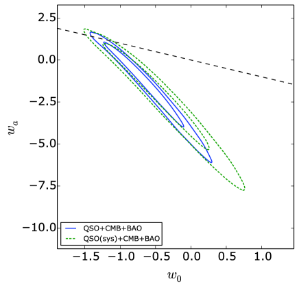
Figure 12: 68.3% and 95.4% confidence regions of the $(w_{0},w_{a})$ plane from QSO, BAO, CMB, and their combination. Zero curvature has been assumed. Points above the dotted line ($w_{0}+w_{a}>0$) violate early matter domination and are disfavored by the data.

where $w_{0}$ and $w_{a}$ are constants and the $\Lambda$CDM model is recovered when $w_{0}=-1$ and $w_{a}=0$. Adding Planck CMB and BAO and to the quasar data gives the 68.3% constraints: $\Omega_{m}=0.320^{+0.029}_{-0.022}$, $w_{0}=-0.606^{+0.578}_{-0.544}$, $w_{a}=-1.207^{+2.335}_{-2.684}$ (without systematics) and $\Omega_{m}=0.330^{+0.032}_{-0.035}$, $w_{0}=-0.439^{+0.830}_{-0.681}$, $w_{a}=-1.816^{+2.878}_{-3.493}$ (with systematics). The constraints on $w_{0}$ and $w_{a}$ are shown in Fig. 12 and Table 2. Note that the combined angular diameter distance data favors a $w_{0}>-1$ and a negative $w_{a}$, which means that dark energy was phantom-like ($w<-1$) in the past, then its EoS crossed the phantom divide, and became quintessence-like ($w>-1$) recently; finally its EoS will become positive in the future. On the contrary, QSO data with $l$ prior favors a $w_{0}<-1$ and a positive $w_{a}$, which means that dark energy was quintessence-like ($w>-1$) in the past, then its EoS crossed the phantom divide, and became phantom-like ($w<-1$) recently; finally the universe will end in a big rip.

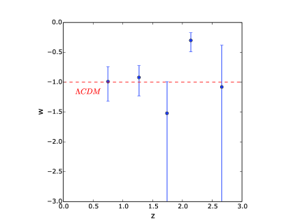
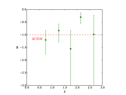
Figure 13: The best fitted $w$ with marginalized $68.3\%$ CL error. The results were obtained assuming a flat universe for the joint data set of QSO, BAO, CMB, with (left panel) and without (right panel) QSO systematics. The QSOs are divided into five groups with $z<1.0$, $1.0<z<1.5$, $1.5<z<2.0$, $2.0<z<2.5$ and $z>2.5$, while BAO and CMB are added to constrain the value of $\Omega_{m}$, considering the well known “geometrical degeneracy” problem. We emphasize that the results are still consistent with the cosmological constant (red-dashed line) at the 68.3% confidence level.

An accurate reconstruction of $w(z)$ can considerably improve our understanding the nature of both dark energy and gravity. In order to reconstruct the evolution of $w(z)$ without assuming a specific form, such model will inevitably include more parameters than $w_{0}-w_{a}$, the number of dark-energy equation-of-state parameters depending on the number of redshift bins (Kowalski et al., 2008). Confined to the sample size of our available quasar data, we carry out the analysis by dividing the full sample into different sub-samples given their redshifts and fitting a constant $w$ in each sub-sample. The redshifts of the QSOs span from $z=0.462$ to $z=2.73$, so we divide the QSOs into five groups with $z<1.0$, $1.0<z<1.5$, $1.5<z<2.0$, $2.0<z<2.5$ and $z>2.5$, respectively. The first group has 30 QSOs with redshifts $z<1.0$, the second group has 51 QSOs with redshifts $1.0<z<1.5$, the third group has 25 QSOs with redshifts $1.5<z<2.0$, the fourth group has 11 QSOs with redshifts $2.0<z<2.5$ and the fifth group contains 3 QSOs. We then fit the cosmic equation of state to each group of QSOs, while the remaining cosmological parameters are fixed at the best-fit values determined by Planck results. The constraints are shown in Fig. 13 and Table 4.

The first group shows a well-constrained equation-of-state parameter from redshift 0.5 to 1.0. Therefore, no evidence of deviation from $w=-1$ is detected from low-redshift quasars, which is in good agreement with the previous findings from Union2.1 SN Ia constraints (Amanullah et al., 2010). The deviation from $\Lambda$CDM is also not obvious in the second and fifth redshift groups. Interestingly, our quasar data favors a transition from $w<-1$ at low redshift to $w>-1$ at higher redshift, a behavior that is consistent with the quintom model allowing $w$ to cross -1. A redshift bin shifts the confidence interval for $w(2.0<z<2.5)$ towards higher $w$, which is typically favored by many scalar field models. As shown in Fig. 13, the transition redshift at which $w$ departing from -1 is apparently located at $z\sim 2.0$, which might be overlooked by the recent analysis with a joint data set including Union2.1 SN, CMB, $H(z)$, RSD (redshift space distortion) and BAO while fixing $w=-1$ at $z>1.5$ (Zhao et al., 2012). More data extending above redshift $z=3$ will be necessary to investigate the dark energy equation-of state parameter in this high redshift region where the uncertainty is still very large.

4 Beyond dark energy

As is well known, a physically profound question to be addressed in the empirical cosmological studies is: does the cosmic acceleration arise from a new energy component with repulsive gravity or a breakdown of General Relativity (GR) on cosmological scales? In this section, we will investigate the constraining power of our quasar sample, concerning different approaches to explain the accelerated expansion of the Universe based on the departure from classical GR. Here we lay the framework for such options and give some examples. In particular we will consider:

• RDE: Ricci dark energy model in a flat universe.

• DGP: Dvali-Gabadadze-Porrati brane world model in a flat universe.

4.1 Ricci dark energy

Other cosmological approaches to describe the dark component have received considerable attention in the past, one of which is holographic dark energy, proposed in the context of the fundamental principle of quantum gravity (Bekenstein, 1981; Gao et al., 2009). Compared with the cosmological constant model, this mechanism may alleviate the well-known coincidence problem and fine tuning problem. The idea, here is that the scale of dark energy is set by a cosmological Hubble horizon scale instead of the Planck length. Choosing an Infrared (IR) cutoff of the quantum field theory as $|R|^{-1/2}$, where $R=6(\dot{H}+2H^{2})$ is the Ricci scalar of the flat Friedman-Robertson-Walker metric, one can derive an effective equivalent of the dark energy density (Gao et al., 2009)

$${\rho_{de}}={3{\beta}M^{2}_{Pl}(\dot{H}+2H^{2})}$$ (16)

where $\beta$ is a constant parameter larger than zero. The Hubble parameter can be derived from the Friedman equation:

$$H^{2}=H_{0}^{2}\left[\frac{2\Omega_{m}}{2-\beta}(1+z)^{3}+(1-{2\Omega_{m}\over 2-\beta})(1+z)^{(4-{2\over\beta})}\right]\,.$$ (17)

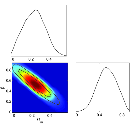
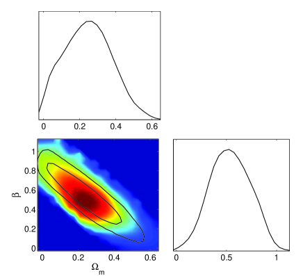
Figure 14: The 2-D regions and 1-D marginalized distribution of RDE model parameters from the quasar sample, without (left panel) and with systematical uncertainties (right panel).

This is a two-parameter model with $\textbf{p}=\{\Omega_{m},~{}\beta\}$. Testing the RDE model with the quasar data, we obtain the following best fits: ${\Omega_{m}}=0.229^{+0.184}_{-0.184}$, $\beta=0.550^{+0.265}_{-0.265}$ (without systematics) and ${\Omega_{m}}=0.240^{+0.210}_{-0.210}$, $\beta=0.520^{+0.365}_{-0.275}$ (with systematics). These results shown presented in Fig. 14 and Table 4 are in agreement with the previous analysis using galactic-scale strong gravitational lensing systems (Biesiada et al., 2011; Cao, Covone & Zhu, 2012), as well as the previous work based on the SNe Ia Constitution compilation, the BAO measurement from the SDSS and the Two Degree Field Galaxy Redshift Survey, and the CMB measurement given by the five-year WMAP observations (Li et al., 2010).

4.2 Higher dimension theories

Past decades have witnessed considerable advances in the modification of General Relativity, as a possible explanation of accelerated expansion of the Universe. One radical proposal is to introduce extra dimensions and allow gravitons to leak off the brane representing the observable universe. Embedding our 4-dimensional spacetime into a higher dimensional bulk spacetime, Dvali & Poratti (2000) proposed the well-known Dvali-Gabadadze-Porrati (DGP) brane world model, in which the leaking of gravity above a certain cosmological scale $r_{c}$ might be responsible for the increasing cosmic expansion rate. Inspired by the DGP example, a general class of “galileon” and massive gravity models has been proposed in the literature (Mortonson et al., 2014). The length at which gravity leaking occurs defines an omega parameter: $\Omega_{r_{c}}=1/(4r^{2}_{c}H^{2}_{0})$, with which the Friedman equation modified as

$$H^{2}=H_{0}^{2}(\sqrt{\Omega_{m}(1+z)^{3}+\Omega_{r_{c}}}+\sqrt{\Omega_{r_{c}}})^{2},$$ (18)

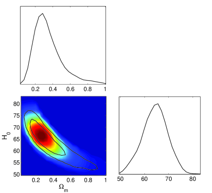
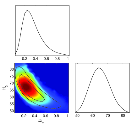
Figure 15: The 2-D regions and 1-D marginalized distribution of DGP model parameters from the quasar sample, without (left panel) and with systematical uncertainties (right panel).

The flat DGP model only contains one free model parameter, ${\theta}=\{\Omega_{m}\}$, which is related to $\Omega_{r_{c}}=\frac{1}{4}(1-\Omega_{m})^{2}$ under assumption of a flat Universe. In order to make a comparison with the $\Lambda$CDM model, we also take the Hubble constant as a free parameter. The best fit value for the mass density parameter in DGP model is $\Omega_{m}=0.285^{+0.255}_{-0.155}$ (without systematics) and $\Omega_{m}=0.248^{+0.335}_{-0.130}$ (with systematics), while the best-fit Hubble constant is $H_{0}=66.2^{+7.4}_{-8.2}\rm{kms}^{-1}\rm{Mpc}^{-1}$ (without systematics) and $H_{0}=64.3^{+11.8}_{-7.6}\rm{kms}^{-1}\rm{Mpc}^{-1}$ (with systematics). These results are presented in Fig. 15 and Table 4. The DGP model is the one for which we obtained the tightest constraints in our analysis. This is due to the simplicity of the model, which depends on only one parameter. In this respect, this is the simplest model, together with the standard flat $\Lambda$CDM. In general, as we already discussed in (Cao & Zhu, 2014), it is to be expected that models with fewer parameters perform better.

From the above considerations, two crucial consequences arise: first, given the current status of cosmological observations including QSOs, there is no strong reason to go beyond the simple, standard cosmological model with zero curvature and a cosmological constant; second, a low value of the Hubble constant is preferred by both the new Planck data and our quasar observations. This consistency between fundamental cosmological parameters constrained from the high redshift CMB measurements $z\sim 1000$ and those from the observations at relatively low redshifts $z\sim 3$ may alleviate the tension between Planck and the SN Ia observations at $z=0$ (Marra et al., 2013; Xia et al., 2013; Li et al., 2014). In fact, projected parameters should presumably be the same from measurements at all $z$ in a given model.

5 Discussion: Improving cosmological constraints by efficiently adding low-redshift clusters

The redshift of intermediate-luminosity quasars ranges between $z=0.46$ and $z=2.73$. Therefore, we also added to the data a set of 25 well-measured angular diameter distances from the galaxy clusters. They have been obtained by considering Sunyaev-Zeldovich effect (SZE) together with X-ray emission of galaxy clusters (De Filippis et al., 2005), where an isothermal elliptical $\beta$ model was used to describe the clusters. The enlargement of $D_{A}(z)$ sample at lower redshifts ($0.142<z<0.890$) improves the assessment of the $w$ parameter that describes the properties of dark energy.

As shown in Fig. 11, adding the cluster data tightens the constraints substantially, giving the improved fitting results on the XCDM model: ${\Omega_{m}}=0.279^{+0.189}_{-0.189}$, $w=-1.066^{+0.614}_{-0.614}$. Speaking in terms of the figure of merit (FoM) — a measure proposed by the Dark Energy Task Force (Albrecht et al., 2006), which is equal to the inverse of the area of the 95% confidence contour in the parameter plane, we find that this combined data set improves the constraint on $w$ by 30%. Considering the redshift coverage of these two astrophysical probes, the combination of high-redshift quasars and low-redshift clusters may provide an important source of angular diameter distances, in addition to the previously studied probes including strongly gravitationally lensed systems (Biesiada, Piórkowska, & Malec, 2010; Biesiada et al., 2011; Cao et al., 2012, 2015b) or X-ray gas mass fraction of galaxy clusters (Allen et al., 2004, 2008).

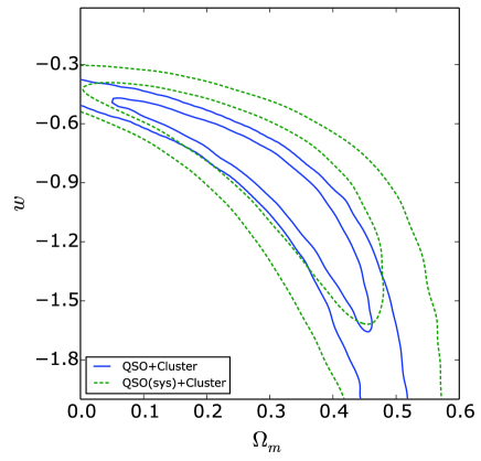
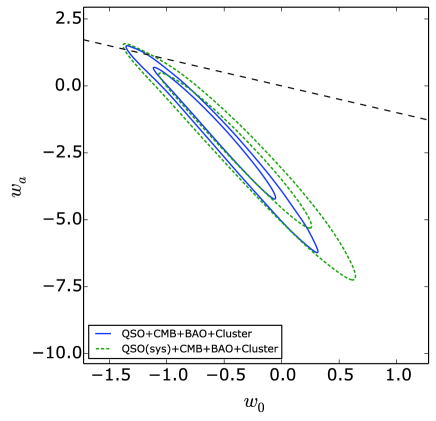
Figure 16: Best-fit confidence regions in the $\Omega_{m}$-$w$ and $w_{0}-w_{a}$ plane from quasars combined with angular diameter distance measurements from cluster observations.

Now we will show how the combination of most recent and significantly improved cosmological observations can be used to study the cosmic equation of state. We consider four background probes which are directly related to angular diameter distances: intermediate-luminosity quasar data (QSO), Sunyaev-Zeldovich effect (SZE) together with X-ray emission of galaxy clusters, baryonic acoustic oscillations (BAO), and CMB observations. The first two probes are always considered as individual standard rulers while the other two probes are treated as statistical standard rulers in cosmology. Results concerning the constraints on the CPL model parameters are displayed in Fig. 16, with the best fit $\Omega_{m}=0.320^{+0.025}_{-0.022}$, $w_{0}=-0.532^{+0.488}_{-0.579}$, $w_{a}=-1.686^{+2.424}_{-2.506}$ (without systematics) and $\Omega_{m}=0.329^{+0.032}_{-0.033}$, $w_{0}=-0.375^{+0.637}_{-0.690}$, $w_{a}=-2.330^{+2.868}_{-2.964}$ (with systematics). At 68.3% C.L., we find that this model is still compatible with $\Lambda$CDM, i.e. the case ($w_{0}=-1$; $w_{a}=0$) typically lies within the 1$\sigma$ boundary. In this context, it is clear that collection of more complete observational data concerning angular diameter distance measurements does play a crucial role (Cao & Zhu, 2014).

6 Summary and conclusions

In this paper, we have presented a newly compiled data set of 120 milliarcsecond compact radio-sources representing intermediate-luminosity quasars covering the redshift range $0.46<z<2.76$. These quasars show negligible dependence of their linear size on the luminosity and redshift ($|n|\simeq 10^{-3}$, $|\beta|\simeq 10^{-4}$) and thus represents, in the standard model of cosmology, a fixed comoving-length of standard ruler. We implemented a new cosmology-independent technique to calibrate the linear size of this standard ruler. In particular, we used the technique of Gaussian processes to reconstruct the Hubble function $H(z)$ as a function of redshift from 15 measurements of the expansion rate obtained from age estimates of passively evolving galaxies. This reconstruction enabled us to derive the angular diameter distance to a certain redshift $z$, and thus calibrate the liner size of radio quasars. More importantly, we found $l_{m}=11.03\pm 0.25$ pc is the typical radius at which AGN jets become opaque at the observed frequency $\nu\sim 2$ GHz. Our measurement of this linear size is also consistent with both the previous and most recent radio observations at other different frequencies, in the framework of the BK79 conical jet model.

Then this new quasar sample was used to investigate the properties of dark energy. In the framework of flat $\Lambda$CDM model, a high value of the matter density parameter, $\Omega_{m}=0.322^{+0.244}_{-0.141}$, and a low value of the Hubble constant, $H_{0}=67.6^{+7.8}_{-7.4}\;\rm{kms}^{-1}\rm{Mpc}^{-1}$ are obtained, which is in excellent agreement with the CMB anisotropy measurements by Planck. For the constant $w$ of a dynamical dark-energy model, we obtained ${\Omega_{m}}=0.309^{+0.215}_{-0.151}$, $w=-0.970^{+0.500}_{-1.730}$ at 68.3% CL, which demonstrates no significant deviation from the concordance $\Lambda$CDM model. Consistent fitting results were also derived for other cosmological mechanisms explaining the cosmic acceleration, including the Ricci dark energy model and Dvali-Gabadadze-Porrati (DGP) brane world model. Moreover, we reconstructed the dark-energy equation-of-state parameter from different quasar sub-sample, and investigated the evolution of $w$ in the redshift range $0.46<z<2.76$. No evidence of deviation from $w=-1$ was detected from low-redshift quasars, which is in good agreement with the previous findings from SN Ia constraints (Amanullah et al., 2010; Suzuki et al., 2012). Interestingly, the most likely reconstruction using our quasar data favors the transition from $w<-1$ at low redshift to $w>-1$ at higher redshift, a behavior that is consistent with the quintom model which allows $w$ to cross -1. The transition redshift at which $w$ departs from -1 is located at $z\sim 2.0$, which might be overlooked by the previous analysis fixing $w=-1$ at $z>1.5$. After adding constraints from the galaxy cluster measurements ($0.142<z<0.890$), we provide a much tighter limit on the EoS parameter: $w=-1.066^{+0.614}_{-0.614}$. Considering the redshift coverage of these two astrophysical probes, the combination of high-redshift quasars and low-redshift clusters may provide an important source of angular diameter distances. In order to asses the reliability of the above results with intermediate-luminosity quasars, the effect of several systematics on the final cosmological fits, due to the uncertainties of the linear size scaling factor ($l$) as well as the dependence of $l_{m}$ on the luminosity and redshift ($\beta$, $n$), were also extensively studied in our cosmological analysis. Our findings revealed that the reduction of the above uncertainties will lead to more stringent cosmological fits, which motivates the future use of VLBI observations based on better uv-coverage to improve constraints on $l$, $\beta$, and $n$ (Pushkarev & Kovalev, 2015).

As a final remark, we point out that the sample discussed in this paper is based on VLBI images observed with various antenna configurations and techniques for image reconstruction. Our analysis potentially suffers from this systematic bias, and taking it fully into account will be included in our future work. To fully utilize the potential of current and future VLBI surveys to constrain cosmology, it will be necessary to reduce systematic errors significantly. The largest current source of systematic uncertainty is calibration. Calibration uncertainties can be split into uncertainties related to the primary standard, and uncertainties in the determination of the value of $l$, the linear size of this standard rod. In principle, the first uncertainty can be reduced by multi-frequency VLBI observations of more compact radio quasars with higher sensitivity and angular resolution (Cao et al., 2017b), while the reduction of the second uncertainty should turn to more efficient distance reconstruction technique. In this paper, we have applied only one particular non-parametric method based on Gaussian processes, to reconstruct angular diameter distances from 24 cosmic chronometer measurements at $z\leq 1.2$. Application of new distance-reconstruction techniques to future VLBI quasar observations of high angular resolutions, will allow us to cross-calibrate the quasar systems and significantly reduce the systematic errors.

The QSO data set presented here and future complementary data sets will help us to explore these possibilities. The approach, introduced in this paper, would make it feasible to build a significantly larger sample of standard rods at much higher redshifts. With such a sample, we can further investigate constraints on the cosmic evolution as well as possible evidence for dynamical dark energy.

Table 1: Compilation of intermediate-luminosity quasars : Column (1): source name; (2): angular size in milliarcseconds; Column (3): uncertainty in angular size; Column (4): total radio flux density at 2.29 GHz (Jy); Column (5): spectral index; Column (6): optical counterpart (Q - Quasar; PQ - Probable QSO).

Source	$z$	$\theta$	$\sigma_{\theta}$	S	$\alpha$	Type	Source	$z$	$\theta$	$\sigma_{\theta}$	S	$\alpha$	Type
P 2351-006	0.462	2.743	0.027	2.49	-0.1	Q	P 2326-477	1.299	2.07	0.047	2.48	0	Q
3C 279	0.5362	1.454	0.052	11.8	0.1	Q	P 0448-392	1.302	1.387	0.064	0.89	0	Q
P 0252-549	0.539	1.049	0.077	1.94	0.1	Q	P 1449-012	1.319	1.682	0.064	0.803	-0.1	Q
P 1136-13	0.558	1.974	0.048	3.4	-0.3	Q	P 2312-319	1.323	0.528	0.135	0.746	-0.3	Q
P 0403-13	0.574	2.399	0.077	4	0.1	Q	P 1327-311	1.326	0.438	0.863	0.5	0.1	Q
P 0920-39	0.591	1.933	0.097	2.1	-0.2	Q	P 1615+29	1.339	1.608	0.117	0.62	-0.2	Q
3C 345	0.5928	1.525	0.041	7.6	0	Q	P 1831-711	1.356	1.46	0.058	1.364	-0.2	Q
GC 1104+16	0.632	1.762	0.15	1.1	-0.1	Q	P 0522-611	1.4	1.168	0.096	0.722	-0.1	Q
P 0113-118	0.67	2.218	0.108	2.7	-0.1	Q	P 0005-239	1.407	0.758	0.14	0.59	-0.1	Q
P 2329-415	0.6715	1.292	0.208	1.1	-0.1	Q	P 2320-035	1.41	0.596	0.171	0.79	-0.1	Q
GC 2251+13	0.673	1.972	0.11	1.1	-0.3	Q	GC 0820+56	1.417	0.424	0.114	0.958	-0.3	Q
P 2344+09	0.677	1.904	0.075	1.9	-0.2	Q	GC 0805+41	1.42	1.481	0.306	0.7	-0.3	Q
1803+78	0.68	1.244	0.129	2.6	-0.1	Q	P 1532+01	1.435	1.172	0.074	1.19	-0.3	Q
0651+82	0.71	1.454	0.245	1.3	0	Q	P 2335-18	1.446	1.81	0.168	0.725	-0.3	Q
P1354+19	0.72	1.415	0.074	1.8	-0.1	Q	P 1030-357	1.455	1.718	0.073	0.682	-0.2	Q
GC 1636+47	0.74	1.139	0.076	1.06	-0.1	Q	AO 0952+17	1.472	1.484	0.223	1	-0.3	Q
P 1237-10	0.752	1.518	0.058	1.63	-0.2	Q	GC 2253+41	1.476	1.327	0.19	1.5	-0.3	Q
P 2135-248	0.819	0.897	0.304	0.7	-0.2	Q	P 0524-460	1.479	1.784	0.059	0.895	0.1	Q
3C 179	0.846	1.953	0.144	1.7	-0.3	Q	P 2052-47	1.489	1.292	0.082	1.05	-0.3	Q
P 0915-213	0.847	1.758	0.094	0.6	-0.1	Q	P 0220-349	1.49	1.243	0.059	0.6	0	Q
GC 1213+35	0.857	1.73	0.183	1.2	-0.3	Q	P 2058-297	1.492	0.87	0.429	0.5	-0.2	Q
P 0454-46	0.858	2.094	0.049	2.439	-0.2	Q	4C 46.29	1.5586	2.446	0.216	0.7	0.1	Q
P 1252+11	0.871	1.635	0.249	0.8	-0.2	Q	P 2227-08	1.5595	1.038	0.109	1.3	-0.1	Q
P 1055+01	0.888	1.144	0.059	2.87	0	Q	P 0406-127	1.563	0.796	0.168	0.58	0.1	Q
P 0537-441	0.894	1.149	0.041	3.777	0.1	Q	P 0837+035	1.57	1.497	0.1	0.65	-0.3	Q
P 0537-158	0.947	1.747	0.087	0.64	-0.1	Q	P 1104-445	1.598	1.743	0.081	1.06	0.1	Q
P 2354-11	0.96	1.661	0.121	1.5	-0.2	Q	P 1351+021	1.6077	1.788	0.034	0.347	-0.3	Q
P 1933-400	0.965	1.81	0.063	1.308	0.1	Q	P 0127+145	1.6301	1.788	0.051	0.579	-0.2	Q
GC 0237+04	0.978	0.568	0.426	0.8	0.1	Q	P 1130+009	1.633	0.659	0.203	0.33	0	Q
P 0208-512	0.999	1.031	0.051	3.679	-0.2	Q	P 0229-398	1.646	1.431	0.093	0.629	0.1	Q
P 0355-483	1.016	1.517	0.033	0.62	-0.1	Q	NRAO 512	1.66	1.245	0.214	1.1	0.1	Q
P 0906+01	1.018	1.794	0.081	0.76	-0.2	Q	P 0922+005	1.72	1.005	0.108	0.94	0	Q
P 0130-17	1.02	1.544	0.197	1	0	Q	P 0202-17	1.74	1.464	0.124	1.2	0	Q
OJ 320	1.025	1.552	0.122	1.2	0	Q	P 1148-171	1.751	1.602	0.205	0.9	-0.3	Q
P 1348-289	1.034	1.797	0.163	1	-0.3	PQ	DW 1403-08	1.763	1.629	0.139	0.73	-0.3	Q
P 2356+196	1.066	1.155	0.453	0.6	0.1	Q	P 2320-021	1.774	1.25	0.191	0.33	0	Q
GC 1514+19	1.07	0.76	0.07	0.525	0	PQ	P 0108-079	1.776	0.66	0.15	1.054	-0.2	Q
P 0122-00	1.08	1.529	0.16	1.3	-0.2	Q	P 1451-400	1.81	1.136	0.047	0.734	-0.2	Q
GC 1144+40	1.088	1.399	0.258	0.9	-0.2	Q	P 1034-374	1.821	0.518	0.082	0.567	-0.3	Q
GC 1335+55	1.0987	0.88	0.581	0.6	-0.2	Q	P 0805-07	1.837	0.85	0.495	1.1	0.1	Q
P 2303-052	1.139	1.638	0.086	0.567	-0.3	Q	0633+73	1.85	1.635	0.307	0.9	-0.3	Q
P 1210+134	1.141	1.727	0.053	0.514	-0.1	Q	OK 492	1.873	1.13	0.286	1.1	0.1	Q
P 2329-16	1.153	1.758	0.054	1.2	0.1	Q	OP-192	1.89	1.537	0.059	1.17	0.1	Q
P 1438-347	1.159	1.277	0.069	0.517	-0.2	Q	OH-230	1.9	1.396	0.194	0.7	-0.2	PQ
P 2332-017	1.184	1.485	0.048	0.57	-0.3	Q	GC 1656+34	1.939	1.526	0.163	0.6	-0.2	Q
P 1127-14	1.187	1.611	0.089	0.79	0	Q	P 0048-071	1.975	1.207	0.094	0.712	-0.1	Q
P 2329-384	1.202	1.099	0.081	0.796	-0.2	Q	GC 0119+24	2.025	1.7	0.279	0.7	0.1	Q
P 1004-018	1.212	1.254	0.088	0.64	0.1	Q	OF 036	2.048	1.901	0.148	0.8	-0.1	Q
QC 08211+39	1.216	2.622	0.085	1.9	-0.2	Q	P 0226-038	2.055	1.595	0.057	0.809	-0.3	Q
OV 591	1.22	2.032	0.147	1.4	-0.1	Q	GC 1325+43	2.073	1.422	0.368	0.6	-0.3	PQ
P 1823-455	1.244	1.38	0.064	0.588	-0.3	Q	P 2319+07	2.09	1.916	0.132	0.9	0	Q
1150+81	1.25	2.44	0.151	1	-0.1	Q	P 1116+12	2.118	0.564	0.664	0.5	-0.3	Q
VRO 40.09.02	1.252	2.109	0.111	1.7	0	Q	P 2145-17	2.13	2.264	0.048	0.834	-0.1	PQ
GC 1020+40	1.254	1.544	0.19	1.2	-0.3	Q	P 1020+191	2.136	1.449	0.077	0.57	-0.3	Q
GC 0537+53	1.275	1.046	0.381	0.8	-0.3	Q	P 0642-349	2.165	1.097	0.223	1.2	0.1	Q
P 0514-16	1.278	1.883	0.146	0.7	-0.1	Q	P 1032-199	2.198	1.434	0.036	1.082	0.1	Q
P 0405-385	1.285	0.979	0.111	2.2	0.1	Q	P 2314-409	2.448	1.676	0.045	0.525	-0.3	Q
OR 186	1.29	1.583	0.107	0.87	-0.3	Q	GC 1337+63	2.5584	1.598	0.323	0.6	-0.2	Q
GC 0707+47	1.292	0.517	0.77	0.8	-0.3	Q	P 0329-255	2.685	1.506	0.101	0.417	-0.1	Q
P 0511-220	1.296	1.2	0.187	1.3	0.1	PQ	P 0136+176	2.73	1.252	0.132	0.52	0	PQ

Table 2: Measurements of the linear size of AGN compact structure at different frequencies. ILQSO denotes Intermediate-Luminosity Quasars.

Frequency $\nu$	Linear size $l(\nu)$	Target systems	Observational technique	Ref
$\nu=2$ GHz	$l=11.03\pm 0.25$ pc	120 ILQSOs	VLBI	This paper
$\nu=4.6$ GHz	$l=5.9\pm 5.0$ pc	Blazar 2200+420	VLBA	O’Sullivan & Gabuzda (2009)
$\nu=5$ GHz	$l=5.59\pm 0.07$ pc	ILQSO (J1611+0844)	VLBI	Frey et al. (2010)
$\nu=5.1$ GHz	$l=5.4\pm 4.5$ pc	Blazar 2200+420	VLBA	O’Sullivan & Gabuzda (2009)
$\nu=7.9$ GHz	$l=2.5\pm 0.7$ pc	Blazar 2200+420	VLBA	O’Sullivan & Gabuzda (2009)
$\nu=8.9$ GHz	$l=2.5\pm 0.6$ pc	Blazar 2200+420	VLBA	O’Sullivan & Gabuzda (2009)
$\nu=12.9$ GHz	$l=1.9\pm 0.4$ pc	Blazar 2200+420	VLBA	O’Sullivan & Gabuzda (2009)
$\nu=15.4$ GHz	$l=1.6\pm 0.3$ pc	Blazar 2200+420	VLBA	O’Sullivan & Gabuzda (2009)
$\nu=22.2$ GHz	$l=1.1\pm 0.3$ pc	Blazar 2200+420	VLBA	O’Sullivan & Gabuzda (2009)
$\nu=43.1$ GHz	$l=0.5\pm 0.1$ pc	Blazar 2200+420	VLBA	O’Sullivan & Gabuzda (2009)

Table 3: Cosmological parameters $\Omega_{m}$, $w_{0}$, $w_{a}$ and the Hubble constant $H_{0}$ fitted to the QSO data.

Fit	$\Omega_{m}$	$w_{0}$	$w_{a}$	$H_{0}[\rm{km\;s}^{-1}\rm{Mpc}^{-1}]$
	$\Lambda$CDM Model
QSO	$0.322^{+0.244}_{-0.141}$	$-1$(fixed)	$0$(fixed)	$67.6^{+7.8}_{-7.4}$
QSO(sys)	$0.312^{+0.295}_{-0.154}$	$-1$(fixed)	$0$(fixed)	$67.0^{+11.2}_{-8.6}$
QSO+CMB	$0.314^{+0.020}_{-0.020}$	$-1$(fixed)	0(fixed)	$68.76^{+1.95}_{-1.98}$
QSO(Sys)+CMB	$0.313^{+0.021}_{-0.020}$	$-1$(fixed)	0(fixed)	$68.87^{+4.65}_{-4.65}$
QSO+CMB+BAO	$0.306^{+0.016}_{-0.014}$	$-1$(fixed)	0(fixed)	$69.45^{+1.58}_{-1.68}$
QSO(Sys)+CMB+BAO	$0.314^{+0.020}_{-0.018}$	$-1$(fixed)	0(fixed)	$68.79^{+4.58}_{-4.36}$
QSO+CMB+BAO+Cluster	$0.306^{+0.016}_{-0.014}$	$-1$(fixed)	0(fixed)	$69.66^{+1.56}_{-1.58}$
QSO(Sys)+CMB+BAO+Cluster	$0.309^{+0.017}_{-0.015}$	$-1$(fixed)	0(fixed)	$69.04^{+2.79}_{-2.81}$
	XCDM Model
QSO	$0.309^{+0.215}_{-0.151}$	$-0.970^{+0.500}_{-1.730}$	$0$(fixed)	$67.3$(fixed)
QSO(sys)	$0.295^{+0.213}_{-0.157}$	$-1.130^{+0.630}_{-2.120}$	$0$(fixed)	$67.3$(fixed)
QSO+CMB	$0.329^{+0.023}_{-0.022}$	$-0.941^{+0.078}_{-0.083}$	$0$(fixed)	$67.3$(fixed)
QSO(Sys)+CMB	$0.323^{+0.057}_{-0.040}$	$-0.956^{+0.183}_{-0.167}$	$0$(fixed)	$67.3$(fixed)
QSO+CMB+BAO	$0.331^{+0.022}_{-0.022}$	$-0.939^{+0.075}_{-0.075}$	$0$(fixed)	$67.3$(fixed)
QSO(Sys)+CMB+BAO	$0.331^{+0.042}_{-0.035}$	$-0.937^{+0.139}_{-0.134}$	$0$(fixed)	$67.3$(fixed)
QSO+CMB+BAO+Cluster	$0.332^{+0.022}_{-0.022}$	$-0.932^{+0.074}_{-0.075}$	0(fixed)	$67.3$(fixed)
QSO(Sys)+CMB+BAO+Cluster	$0.335^{+0.042}_{-0.034}$	$-0.916^{+0.131}_{-0.131}$	0(fixed)	$67.3$(fixed)
	$w_{z}$CDM Model
QSO+CMB	$0.313^{+0.044}_{-0.024}$	$-0.676^{+0.973}_{-0.707}$	$-0.745^{+2.396}_{-5.501}$	$67.3$(fixed)
QSO(Sys)+CMB	$0.312^{+0.052}_{-0.038}$	$-0.401^{+1.057}_{-0.992}$	$-1.610^{+3.190}_{-6.371}$	$67.3$(fixed)
QSO+CMB+BAO	$0.320^{+0.029}_{-0.022}$	$-0.606^{+0.578}_{-0.544}$	$-1.207^{+2.335}_{-2.684}$	$67.3$(fixed)
QSO(Sys)+CMB+BAO	$0.330^{+0.032}_{-0.035}$	$-0.439^{+0.830}_{-0.681}$	$-1.816^{+2.878}_{-3.493}$	$67.3$(fixed)
QSO+CMB+BAO+Cluster	$0.320^{+0.025}_{-0.022}$	$-0.532^{+0.488}_{-0.579}$	$-1.686^{+2.424}_{-2.506}$	$67.3$(fixed)
QSO(Sys)+CMB+BAO+Cluster	$0.329^{+0.032}_{-0.033}$	$-0.375^{+0.637}_{-0.690}$	$-2.330^{+2.868}_{-2.964}$	$67.3$(fixed)

Table 4: Constraints on equation of state $w$ from the redshift-divided radio quasar data.

EoS parameter	0.46 $<$ z $<$ 1.0	1.0 $<$ z $<$ 1.5	1.5 $<$ z $<$ 2.0	2.0 $<$ z $<$ 2.5	2.5 $<$ z $<$ 2.73
$w[QSO]$	$-0.99^{+0.25}_{-0.33}$	$-0.92^{+0.20}_{-0.31}$	$-1.52^{+0.53}_{-2.14}$	$-0.30^{+0.13}_{-0.19}$	$-1.08^{+0.70}_{-8.92}$
$w[QSO(sys)]$	$-1.20^{+0.38}_{-0.56}$	$-0.83^{+0.26}_{-0.45}$	$-1.55^{+0.73}_{-5.79}$	$-0.30^{+0.17}_{-0.25}$	$-0.98^{+0.75}_{-9.02}$

Table 5: Best fits for different cosmological models from the radio quasar data.

Cosmological models	Cosmological parameters	Cosmological parameters (sys)
Flat cosmological constant	$\Omega_{m}=0.322^{+0.244}_{-0.141}$, $H_{0}=67.6^{+7.8}_{-7.4}km/s/Mpc$	$\Omega_{m}=0.312^{+0.295}_{-0.154}$, $H_{0}=67.0^{+11.2}_{-8.6}\;km/s/Mpc$
Constant $w$	${\Omega_{m}}=0.309^{+0.215}_{-0.151}$, $w=-0.97^{+0.50}_{-1.73}$	${\Omega_{m}}=0.295^{+0.213}_{-0.157}$, $w=-1.13^{+0.63}_{-2.12}$
Ricci dark energy	${\Omega_{m}}=0.229^{+0.184}_{-0.184}$, $\beta=0.550^{+0.265}_{-0.265}$	${\Omega_{m}}=0.240^{+0.210}_{-0.210}$, $\beta=0.520^{+0.365}_{-0.275}$
Dvali-Gabadadze-Porrati	$\Omega_{m}=0.285^{+0.255}_{-0.155}$, $H_{0}=66.2^{+7.4}_{-8.2}km/s/Mpc$	$\Omega_{m}=0.248^{+0.335}_{-0.130}$, $H_{0}=64.3^{+11.8}_{-7.6}km/s/Mpc$

References

- Planck Collaboration XVI (2014) Ade, P. A. R., Aghanim, N., & Armitage-Caplan, C., et al. 2014, A&A, 571, A16
- Planck Collaboration XIII (2016) Ade, P. A. R., Aghanim, N., Arnaud, M., et al. 2016, A&A, 594, A13
- Planck Collaboration XIV (2016) Ade, P. A. R., Aghanim, N., Arnaud, M., et al. 2016, A&A, 594, A14
- Albrecht et al. (2006) Albrecht, A., et al. 2006, arXiv:0609591
- Allen et al. (2004) Allen, S. W., et al. 2004, MNRAS, 353, 457
- Allen et al. (2008) Allen, S. W., et al. 2008, MNRAS, 383, 879
- Amanullah et al. (2010) Amanullah, R., et al. 2010, ApJ, 716, 712
- Anderson et al. (2014) Anderson, L., Aubourg, E., Bailey, S., et al., 2014, MNRAS, 441, 24 [arXiv:1312.4877]
- Barai & Wiita (2007) Barai, P., & Wiita, P. J. 2007, ApJ, 658, 217
- Bekenstein (1981) Bekenstein, J. D. 1981, PRD, 23, 287
- Bonamente et al. (2006) Bonamente, M., et al. 2006, ApJ, 647, 25
- Busti et al. (2014) Busti, V. C., et al. 2014, MNRAS, 441, L11
- Beutler et al. (2011) Beutler, F., Blake, C., Colless, M., et al., 2011, MNRAS, 416, 3017 [arXiv:1106.3366]
- Bennett et al. (2014) Bennett, C. L., Larson, D., Weiland, J. L., & Hinshaw, G. 2014, ApJ, 794, 135
- Biesiada, Piórkowska, & Malec (2010) Biesiada, M., Piórkowska, A., & Malec, B. 2010, MNRAS, 406, 1055
- Biesiada et al. (2011) Biesiada, M., et al. 2011, RAA, 11, 641
- Blandford & Rees (1978) Blandford, R. D. & Rees, M. J. 1978, “Some comments on radiation mechanisms in Lacertids, in BL Lac Objects” (ed. A.M.Wolfe), University of Pittsburgh, Pittsburgh, pp. 328 C341
- Blandford & Königl (1979) Blandford, R. D., & Königl, A., 1979, ApJ, 232, 34
- Buchalter et al. (1998) Buchalter, A., Helfand, D. J., Becker, R. H., & White, R. L., 1998, ApJ, 494, 503
- Cao & Zhu (2011a) Cao, S., & Liang, N. 2011a, RAA, 11, 1199
- Cao & Zhu (2011b) Cao, S., & Zhu, Z.-H. 2011b, China Series G, 54, 2260 [arXiv:1102.2750]
- Cao et al. (2012) Cao, S., et al. 2012, JCAP, 55, 140
- Cao, Covone & Zhu (2012) Cao, S., Covone, G., & Zhu, Z.-H. 2012, ApJ, 755, 516
- Cao & Zhu (2014) Cao, S., & Zhu, Z.-H. 2014, PRD, 90, 083006
- Cao et al. (2015a) Cao, S., et al. 2015a, ApJ, 806, 66
- Cao et al. (2015b) Cao, S., et al. 2015b, ApJ, 806, 185
- Cao et al. (2017a) Cao, S., et al. 2017a, JCAP, 02, 012 [arXiv:1609.08748v2]
- Cao et al. (2017b) Cao, S., et al. 2017b, in preparation
- Chen & Ratra (2003) Chen, G., & Ratra, B. 2003, ApJ, 582, 586
- Chen et al. (2010) Chen, Y., Zhu, Z.-H., Alcaniz, J. S., & Gong, Y. G. 2010, ApJ, 711, 439
- Chevalier & Polarski (2001) Chevalier, M. & Polarski D. 2001, IJMPD, 10, 213
- Chiba & Yoshii (1999) Chiba, M., & Yoshii, Y. 1999, ApJ, 510, 42
- Conley et al. (2011) Conley, A., Guy, J., Sullivan, M., et al. 2011, ApJS, 192, 1
- Daly (1994) Daly, R. A., 1994, ApJ, 426, 38
- Daly & Djorgovski (2003) Daly, R. A., & Djorgovski, S. G. 2003, ApJ, 597, 9
- De Filippis et al. (2005) De Filippis, E., Sereno, M., Bautz, W., Longo, G. 2005, ApJ, 625, 108
- Ding et al. (2015) Ding, X., Biesiada, M., Cao, S., Li, Z. X. & Zhu, Z.-H., 2015, ApJL, 803, L22
- Dvali & Poratti (2000) Dvali, G., Gabadadze, G., & Porrati, M. 2000, PLB, 485, 208
- Eisenstein et al. (1998) Eisenstein, D. J. and Hu, W., 1998, ApJ, 496, 605
- Ellis & Stoeger (1987) Ellis, G. F. R. & Stoeger, W. 1987, ClassQuantGra, 4, 1697
- Freedman et al. (2001) Freedman, W. L., et al. 2001, ApJ, 553, 47
- Frey et al. (2010) Frey, S., et al. 2010, A&A, 524, A83
- Gao et al. (2009) Gao, C., Wu, F., Chen, X.,& Shen, Y. 2009, PRD, 79, 043511
- Gott et al. (2001) Gott, J. R., III, Vogeley, M. S., Podariu, S., & Ratra, B. 2001, ApJ, 549, 1
- Guerra & Daly (1998) Guerra, E. J., & Daly, R. A. 1998, ApJ, 493, 536
- Guerra, Daly & Wan (2000) Guerra, E. J., Daly, R. A., & Wan, L. 2000, ApJ, 544, 659
- Gurvits (1994) Gurvits, L. I., 1994, ApJ, 425, 442
- Gurvits, Kellerman & Frey (1999) Gurvits, L. I., Kellerman, K. I., & Frey, S. 1999, A&A, 342, 378
- Holanda et al. (2013) Holanda, R. F. L., Carvalho, J. C., & Alcaniz, J. S. 2013, JCAP, 04, 027
- Holsclaw et al. (2010a) Holsclaw, T., et al. 2010a PRD, 82, 103502
- Holsclaw et al. (2010b) Holsclaw, T., et al. 2010b, PRL, 105, 241302
- Hopkins & Quataert (2010) Hopkins, P. F., & Quataert, E. 2010, MNRAS, 407, 1529
- Hu & Sugiyama (1996) Hu, W. & Sugiyama, N. 1996, ApJ, 471, 542
- Jackson & Dodgson (1997) Jackson J. C., & Dodgson M. 1997, MNRAS, 285, 806
- Jackson (2004) Jackson, J. C. 2004, JCAP, 11, 7
- Jackson & Jannetta (2006) Jackson J. C., Jannetta A.L., 2006, JCAP, 11, 002
- Jimenez & Loeb (2002) Jimenez, R. & Loeb, A., 2002, ApJ, 573, 37
- Kayser (1995) Kayser, R. 1995, A&A, 294, 21
- Kellermann (1993) Kellermann, K. I. 1993, Nature, 361, 134
- Kowalski et al. (2008) Kowalski, M., et al. 2008, ApJ, 686, 749
- Li et al. (2010) Li, M., Li, X. D., & Zhang, X. 2010, Science China Physics Mechanics & Astronomy, 53 1631
- Li et al. (2014) Li, Z. X., et al. 2014, Science China Physics Mechanics & Astronomy, 57, 381
- Li et al. (2016) Li, Z. X., et al. 2016, PRD, 93, 043014
- Lima & Alcaniz (2002) Lima, J. A. S., & Alcaniz, J. S. 2002, ApJ, 566, 15
- Linder (2004) Linder, E. V. 2004, PRD, 68, 083503
- Lobanov (1998) Lobanov, A. P. 1998, A&A, 330, 79
- Marra et al. (2013) Marra, V., et al. 2013, PRL, 110, 241305
- Meier (2009) Meier, D. L., 2009, in Hagiwara Y., Fomalont E., Tsuboi M., Murata Y., eds, Approaching Micro-Arcsecond Resolution with VSOP-2: Astrophysics and Technology. Vol. 402. ASP Conf. Ser., San Francisco., p. 342
- Moresco et al. (2012) Moresco, M., et al. 2012, JCAP, 1208, 006
- Mortonson et al. (2014) Mortonson, M. J., et al. 2014, arXiv:1401.0046v1
- O’Sullivan & Gabuzda (2009) O’Sullivan, S. P. & Gabuzda, D. C. arXiv:0907.5211v2
- Peebles & Ratra (2003) Peebles, P. J., & Ratra, B. 2003, Rev. Mod. Phys., 75, 559
- Perlmutter et al. (1999) Perlmutter, S., et al. 1999, ApJ, 517, 567
- Podariu et al. (2003) Podariu, S., Daly, R. A., Mory, M. P., & Ratra, B. 2003, ApJ, 584, 577
- Pope et al. (2004) Pope, A. C., et al. 2004, AJ, 148, 175
- Preston et al. (1985) Preston, R. A., Morabito D. D., Williams J. G., Faulkner J., Jauncey D. L., Nicolson G. D., 1985, AJ, 90, 1599
- Pushkarev & Kovalev (2015) Pushkarev, A. B., & Kovalev, Y. Y. 2015, MNRAS, 452, 4274
- Ratra et al. (1988) Ratra, B., & Peebles, P. J. E. 1988, PRD, 37, 3406
- Riess et al. (1998) Riess, A. G., et al. 1998, AJ, 116, 1009
- Riess et al. (2009) Riess, A. G., et al. 2009, ApJS, 183, 109
- Riess et al. (2016) Riess, A. G., Macri, L. M., Hoffmann, S. L., et al. 2016, ApJ, 826, 56
- Ross et al. (2015) Ross, A. J., Samushia, L., Howlett, C., et al., 2015, MNRAS, 449, 835 [arXiv:1409.3242]
- Roukema et al. (2015) Roukema, B., Buchert, T., Ostrowski, J. J. & France, M. J. 2015, MNRAS, 448, 1660
- Roukema et al. (2016) Roukema, B., Buchert, T., Fuji, H. & Ostrowski J. J. 2016, MNRAS, 456, L45
- Sandage (1988) Sandage, A. 1988, ARA&A, 26, 561
- Seikel et al. (2013) Seikel, M., Clarkson, C., & Smith, M. 2012, JCAP, 6, 36
- Shafieloo et al. (2013) Shafieloo, A., et al. 2013, PRD, 87, 023520
- Singal (1993) Singal, A. K. 1993, MNRAS, 263, 139
- Silverman et al. (2009) Silverman, J. D., et al. 2009, ApJ, 695, 171
- Spergel et al. (2003) Spergel, D. N., et al. 2003, AJS, 148, 175
- Suzuki et al. (2012) Suzuki, N., et al. 2012, ApJ, 611, 739
- Thompson, Moran & Swenson (1986, p. 13) Thompson, A.R., Moran, J.M., & Swenson G.W. 1986, Interferometry and Synthesis in Radio Astronomy (John Wiley & Sons, New York)
- Tammann et al. (2008) Tammann, G. A., Sandage, A., & Reindl, B. 2008, A&A Rev, 15, 289
- Verde et al. (2014) Verde, L., Protopapas, P., & Jimenez, R. 2014, Phys. Dark Univ. 5-6, 307
- Vishwakarma (2001) Vishwakarma, R. G. 2001, Classical Quantum Gravity, 18, 1159
- Xia et al. (2013) Xia, J.-Q., et al. 2013, PRD, 88, 063501
- Zhang (2014) Zhang, Y. 2014, arXiv:1408.3897
- Zhao et al. (2012) Zhao, G. B., et al. 2012, PRL, 109, 171301
- Zheng et al. (2016) Zheng, X., Ding, X., Biesiada, M., Cao, S., & Zhu, Z.-H. 2016, ApJ, 825, 1
- Zhu & Fujimoto (2002) Zhu, Z.-H., & Fujimoto, M. K. 2002, ApJ, 581, 1