Planet Four: Terrains - Discovery of Araneiforms Outside of the South Polar Layered Deposits

Abstract

We present the results of a systematic mapping of seasonally sculpted terrains on the South Polar region of Mars with the Planet Four: Terrains (P4T) online citizen science project. P4T enlists members of the general public to visually identify features in the publicly released Mars Reconnaissance Orbiter Context Camera (CTX) images. In particular, P4T volunteers are asked to identify: 1) araneiforms (including features with a central pit and radiating channels known as ‘spiders’); 2) erosional depressions, troughs, mesas, ridges, and quasi-circular pits characteristic of the South Polar Residual Cap (SPRC) which we collectively refer to as ‘Swiss cheese terrain’, and 3) craters. In this work we present the distributions of our high confidence classic spider araneiforms and Swiss cheese terrain identifications in 90 CTX images covering 11$\%$ of the South polar regions at latitudes $\leq$ -75^∘ N. We find no locations within our high confidence spider sample that also have confident Swiss cheese terrain identifications. Previously spiders were reported as being confined to the South Polar Layered Deposits (SPLD). Our work has provided the first identification of spiders at locations outside of the SPLD, confirmed with high resolution HiRISE (High Resolution Imaging Science Experiment) imaging. We find araneiforms on the Amazonian and Hesperian polar units and the Early Noachian highland units, with 75$\%$ of the identified araneiform locations in our high confidence sample residing on the SPLD. With our current coverage, we cannot confirm whether these are the only geologic units conducive to araneiform formation on the Martian South Polar region. Our results are consistent with the current CO₂ jet formation scenario with the process exploiting weaknesses in the surface below the seasonal CO₂ ice sheet to carve araneiform channels into the regolith over many seasons. These new regions serve as additional probes of the conditions required for channel creation in the CO₂ jet process.

]mschwamb.astro@gmail.com

1 Introduction

The seasonal processes sculpting the Martian South Polar region are driven by the sublimation and deposition of carbon dioxide (CO₂) ice. A significant portion of the Martian atmosphere, of which CO₂ is the predominant species, freezes or snows out on to the winter pole during the fall and winter. During the spring and summer, all or part of the deposited CO₂ returns to the atmosphere [38, 25, 59, 19]. This is observed by the large seasonal variations in atmospheric pressure, with amplitudes up to 25$\%$, first measured by the Viking landers [22, 83]. Combined multi-season gravity field observations from Mars Global Survey (MGS), Mars Odyssey, and Mars Reconnaissance Orbiter (MRO) point to approximately 12 to 16$\%$ of the mass of the entire Martian atmosphere solidifying out on to the surface of the winter pole [19]. This cycle is directly linked to the current Martian climate. Thus, studying how the Martian South Pole region’s inventory of CO₂ ice changes and evolves throughout the season and from Mars year to Mars year provides insight into processes driving Mars’ climate and atmosphere.

The Martian South Pole’s CO₂ inventory can be divided into buried ice deposits and two broad surface ice caps, the temporary seasonal cap and the more permanent South Polar Residual Cap (SPRC). The buried CO₂ deposits vary from tens to thousands of meters in thickness and are topped with a 10-60 m layer of water ice. The mass of these buried CO₂ ice reservoirs if sublimated is estimated to double the planet’s current atmospheric pressure [7]. These CO₂ ice deposits are located below the South Polar Layered Deposits (SPLD) [53, 7]. The SPLD is comprised mostly of bands of dust and water ice in addition to the buried subsurface CO₂ ice reservoirs [14, 13, 53, 7]. The SPLD is thought to have formed through repeated deposition linked to Mars’ orbital/obliquity variations produced by the planet’s Milankovitch cycles [21]. Recent modeling of Mars’ climate variations is also able to produce wide-spread deposition of CO₂ on the South Polar region, [53, 7], indicating the formation of the buried CO₂ reservoirs is also linked to Mars’ Milankovitch cycles.

The SPRC is located between -84 to -89 degrees latitude and 220 E and 50 degrees E longitude. It is primarily made of carbon dioxide ice [38, 10, 80, 77]. The extent of the SPRC has been observed to expand and to retreat during various Mars years, but the structure as a whole survives past the spring and summer season [29, 25, 34, 24, 6, 26]. The temporary seasonal ice sheet on the other hand completely sublimates away by the end of the Southern summer [29, 57, 28, 41, 65, 54, 59]. The SPRC is thicker and higher albedo than most of the temporary seasonal cap, with thickness ranging between $\sim$0.5 and 10 meters [78, 10, 77, 75]. The surface of the SPRC is heavily eroded with smooth edged quasi-circular flat bottomed pits, mesas, troughs, and other depressions [25, 78, 43, 45, 79, 77, 76, 75]. [77] and [75] provide a detailed description of morphologies of the SPRC based on orbital imagery. The SPRC pits, depressions, and troughs have been observed to change in depth and areal coverage indicative of active mass loss [43, 77, 76, 9]. Mass balance modeling suggests these errosional features are due to the uneven sublimation and deposition of CO₂ ice on the SPRC [10, 4, 75].

The seasonal cap is a temporary CO₂ ice sheet that extends from the pole to latitudes as far north as -50^∘, and in cold protected patches to -22^∘ [68, 26]. Mars Orbiter Laser Altimeter (MOLA) observations place the seasonal ice sheet thickness at $\sim$0.9-2.5 m [71, 1], with compaction decreasing the thickness over the winter [49]. A portion of the seasonal cap covers an area referred to as the cryptic terrain, areas where the albedo is low but has the temperatures of CO₂ ice ($\sim$150 K), indicating the presence of semi-translucent slab ice [33, 31]. Every Mars year, the spring sublimation of the seasonal polar cap results in the formation of CO₂ jets and dark seasonal fans. In the generally accepted CO₂ jet model, sunlight penetrates through the slab of CO₂ ice to the base regolith layer, heating the ground [30, 57, 32, 31, 58, 73, 63, 55, 74]. This results in sublimation at the base of the ice sheet, forming a trapped layer of gas between the ice and the regolith. The trapped CO₂ gas is thought to exploit any weaknesses in the ice above, breaking through to the top of the ice sheet as a CO₂ jet. Dust and dirt from below the ice sheet are carried by the jet and expelled into the atmosphere. It is thought that the local surface winds carry the particles as they settle onto the top of the ice sheet producing the dark fan-like streaks and blotches observed from orbit during the spring and summer. When the seasonal cap disappears, the majority of the seasonal fans and blotches fade and blend into the background regolith, further supporting the idea that the fan material is the same as the regolith below the ice sheet [32, 73, 60]. Recent laboratory experiments by [27] were able to trigger dust eruptions from a layer of dust inside a CO₂ ice slab under Martian conditions, lending further credence to the proposed CO₂ jet and fan production model.

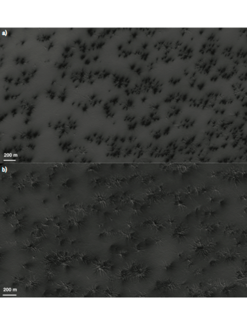
Figure 1: Examples of araneiform features imaged by HiRISE. Figures a and b show radially-organized 1-m deep channels emanating from a slightly deeper center. More colloquially these dendritic channel structures have been referred to as ’spiders.’ At these times the terrain in the images was covered by a semi-translucent seasonal layer of CO₂ ice. The araneiforms are channels below the ice carved into the underlying regolith. Seasonal fans of fine particles from ruptures in the ice are deposited on top of the seasonal ice layer are present and visible in the images as the dark black fan-like and more blotch-like features. The location of seasonal fans are not always directly associated with araneiform channels, but araneiform channels have been observed to have seasonal fans emanating at the surface of the ice sheet above their positions at HiRISE resolution [20]. From top to bottom: ESP$\_$020558$\_$0930 (L_s=198.9^∘) and ESP$\_$011420$\_$0930 (L_s=184.3^∘).

Small pits in the surface with radiating channels a few meters deep, colloquially known as ‘spiders,’ have also been identified in spacecraft imagery in many of the same areas as where the seasonal fans are present [30, 57, 32, 20]. Spiders range in diameter from tens of meters to 1 km[20]. Many seasonal fans appear to originate from the spider ‘legs’, but not all observed fans do [57, 20]. With the arrival of MRO and the HiRISE [High Resolution Imaging Science Experiment; 50] camera, with a pixel scale of $\sim$30 cm/pixel at 300 km altitude, new morphologies of spider-like channels have been found [20]. This includes ‘lace terrain’, where the dendritic-like channels of spiders are connected with no visible central pit. Spiders and these other spider-like dendritic channels are now collectively referred to as araneiforms [20], and they are thought to form via the CO₂ jet process [30, 57, 32, 31, 58, 73, 63, 55, 74, 15]. A sample of araneiform features from high resolution imaging is shown in Figures 1 and 2.

Through a survey of over 5,000 Mars Orbiter Camera (MOC) Narrow Angle (NA) [44, 46] images, [57] linked the presence of CO₂ slab ice with araneiform formation. They found that araneiforms are located in regions where the seasonal CO₂ ice cap becomes cryptic for at least some part of the Southern spring and summer, lending further support to the idea that araneiforms are gradually carved into the ground by the trapped CO₂ gas during the formation of CO₂ jets. [57] also found that spiders are confined to the top of the SPLD. The erosional mechanism forming araneiforms is a slow process; over many spring/summer seasons the trapped gas underneath the sublimating ice sheet carves these features into the top of the SPLD. Estimates from modeling by [58] and recent HiRISE observations of araneiform channel formation by [62] place araneiform ages at $10^{3}-10^{4}$ years.

[57] argue that with their areal coverage they would have seen spiders in the MOC NA images they visually inspected outside of the SPLD. Why araneiforms appear to only be constrained to the top of the SPLD is an open question. [57] postulate that araneiforms may be restricted to the SPLD because the SPLD is composed of more loosely consolidated material than other geologic units on the South Polar region [81]; perhaps making it easier to erode by the CO₂ gas than in other areas. In the past decade with the arrival of the Context Camera [CTX; 42] aboard MRO, many areas of the South Polar region have been imaged multiple times each Mars Year with 6-8 m per pixel scale, better resolution than some of the MOC NA observations searched by [57] and also in areas that were not covered in the original [57] search.

More widely distributed coverage will allow us to expand upon the previous maps of araneiform locations. With newly discovered araneiform locales, we can further explore what conditions (weather, types of terrain, erodibility of the ground, latitude, and other surface and climate properties) are key for araneiform development through comparison to previous regions monitored by HiRISE for 5 Mars Years such as the informally named ‘Manhattan’ and ‘Inca City’ [e.g. 20, 64, 62]. We can also compare the distribution of araneiforms to other features on the South Polar region produced by the sublimation of CO₂ ice, such as the Swiss cheese terrain. In addition, finding new areas with past CO₂ jets and seasonal fans activity is an important resource for future mission and target planning.

We created Planet Four: Terrains (P4T), an online citizen science project which enlists the general public to map the locations of 1) araneiforms (including features with a central pit and radiating channels known as ‘spiders’); 2) erosional depressions, troughs, mesas, ridges, and quasi-circular pits characteristic of the South Polar Residual Cap (SPRC) which we collectively refer to as ‘Swiss cheese terrain’, and 3) craters in publicly available CTX observations. The human brain is ideally suited for this task and with very little training is easily capable of identifying these features in orbital images of Mars. Previous studies have visually identified features like araneiforms, Swiss cheese terrain, or recurring slope lineae using a single person or groups of researchers reviewing observations taken from orbit [e.g. 57, 79, 77, 20, 52, 51]. With the Internet, tens of thousands of people across the globe can be enlisted in such tasks to create a larger sample and in particular review images typically in more detail than in the time a single researcher or group of researchers can. This citizen science or crowd-sourcing approach, where independent assessments from multiple non-expert classifiers are combined, has been applied to nearly all areas in astronomy and planetary science [48] (see references therein) including galaxy morphology [40, 82], exoplanet searches [17, 69], circumstellar disk identification [36], and crater counting [66, 8].

In this Paper we present the first results from P4T, examining the distribution of araneiforms with spider morphology and comparing to the Swiss cheese terrain on the Martian South Pole. In Section 2 we provide an overview of the image dataset used in this work. We describe the P4T project and web classification interface in Section 3. In Section 4 we detail the process of combining the multiple volunteer assessments to identify surface features in the Mars image data reviewed. In Section 5 we present our map of spider locations within  15^∘ of the Martian South Pole, and in Section 6 we compare these locations to the distribution of secure Swiss cheese terrain identifications. We report the discovery of araneiforms outside of the SPLD and in Section 7 present higher resolution confirmation imaging from HiRISE. In Section 8 we discuss the implications of this result for the CO₂ jet model. All place names referred to in this Paper are informal and not approved by the International Astronomical Union. All reported latitudes are areographic, and all longitudes are reported in reference to East longitude. Full machine-readable versions of the catalogs and tables presented in this Paper are also available from https://www.zooniverse.org/projects/mschwamb/planet-four-terrains/about/results.

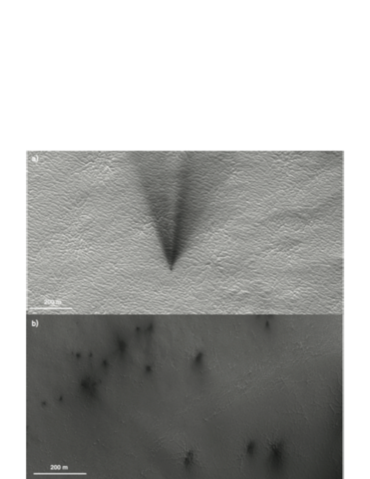
Figure 2: Connected araneiforms, a diffferent end-member of the spectrum of araneiforms with no centralized channel organization, but bearing the characteristic hallmark of sinuous channels with seasonal fans as imaged by HiRISE. At these times the terrain in the images was covered by a semi-translucent seasonal layer of CO₂ ice. The araneiforms are channels below the ice carved into the underlying regolith. Seasonal fans of fine particles from ruptures in the ice are deposited on top of the seasonal ice layer are present and visible in the images as the dark black fan-like and more blotch-like features. The location of seasonal fans are not always directly associated with araneiform channels, but araneiform channels have been observed to have seasonal fans emanating at the surface of the ice sheet above their positions at HiRISE resolution [20]. From top to bottom: PSP$\_$002850$\_$0935 (L_s=195.4^∘) and ESP$\_$038022$\_$0985 (L_s=191.2^∘).

2 Dataset

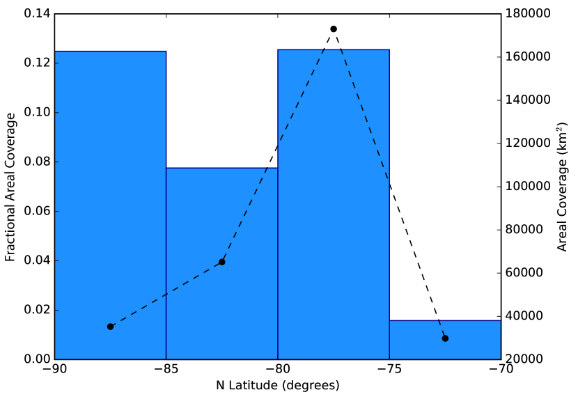
Figure 4: The fractional areal coverage of the Martian South Polar region (blue in the online version) histogram of the P4T CTX images searched in 5-degree latitude bins. The dashed line shows the areal coverage in km².

For our analysis, we used publicly available observations from CTX [42] aboard MRO obtained from NASA’s Planetary Data System (PDS). CTX has widespread coverage of the Martian south polar region at a variety of solar longitudes (L_S). The camera provides the best balance between resolution and areal coverage with a single observation typically spanning a $\sim$30$\times$60 km swath at 6 m/pixel spatial scale. [57] found araneiforms were constrained to the SPLD; we thus restricted our study to CTX observations with latitudes southward of -75^∘ latitude in order to encompass the majority of the SPLD defined by [72]. We selected 90 CTX images for review on P4T for this work. The area covered by our search images is shown in Figure 3. We have surveyed CTX observations covering 303,192 km² within -70^∘ latitude and 11$\%$ of the South Polar region within -75^∘ N. The areal coverage of the surveyed CTX images as a function of latitude is shown in Figure 4. The observing circumstances and planetographic coordinates of the selected CTX observations are summarized in Table LABEL:tab:CTXobs.

2.1 CTX Image Selection

We provide a brief overview of the process used to select the 90 CTX images used in this analysis. Since araneiform formation takes thousands of Mars years [58, 62], we do not restrict ourselves to a single Mars year. We chose from publicly available CTX observations taken between October 2007 and October 2013, Mars years (MY) 28-32 according to the convention defined by [12] and [56]. The CO₂ jet process on the seasonal ice cap produces fans which appear as dark streaks and blotches in CTX images throughout the Southern spring and summer. We attempted to select CTX observations of locations where the CO₂ seasonal cap had already sublimated in order to reduce the number of obscuring fans. The extent of the seasonal CO₂ cap in latitude and longitude varies as as a function of L_S. We used previous thermal measurements of the South polar region [59] and a brief visual inspection of the CTX images to determine latitude/L_S ranges that were ice free.

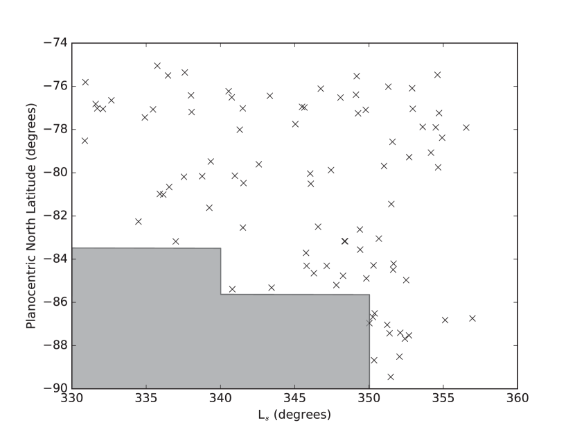
Figure 5: The distribution of center latitudes for the 90 CTX images selected as a function of L_S. The greyed region represents the excluded latitudes chosen to avoid as much as possible the presence of the dark seasonal fans on the seasonal cap.

With the remaining CTX images that pass the selection cuts, we attempt to achieve as widespread coverage as possible distributed across the South Polar region. We divide the South polar region southward of -75 ^∘ latitude into 30^∘ longitude and 5^∘ latitude bins. The 90 CTX images used in this study were randomly selected from each bin with slightly more images picked with field centers between -85^∘ and -75^∘ latitude. The final area covered by our search images is shown in Figure 3. Figure 5 shows the latitude distribution of the selected CTX images for this study as a function of L_S.

A visual inspection of the final 90 CTX images selected finds that majority of the images are free from clouds or obscuring seasonal fans. We do not have criteria for assessing the fraction of cloud cover, atmospheric opacity, or presence of seasonal fans in each of the selected CTX images used in our search. Thus the lack of a positive identification of araneiforms, Swiss Cheese Terrain, or craters by P4T does not necessarily mean the feature is not present in a given CTX image. Our analysis instead identifies locations where araneiforms, Swiss Cheese Terrain, and craters are confidently identified by P4T but does not provide a complete sample.

2.2 CTX Image Processing and P4T Subject Creation

The selected full frame CTX images searched by P4T are subdivided into smaller subimages that are subsequently presented to volunteers on the P4T website. The raw CTX image products or Experiment Data Records (EDRs) were processed with Python using the United States Geological Survey’s (USGS) Integrated Software for Imagers and Spectrometers (ISIS) [ISIS-3 2, 5] and the ISIS-3 python wrapper Pysis. After radiometric calibration and noise removal, the CTX frames were divided into smaller non-overlapping 800$\times$600 pixel ($\sim$4.8$\times 3.6$ km) PNG (Portable Network Graphics) subimages to be presented on the P4T website. We refer to these subimages as ‘subjects.’ The PNG exporter from the ISIS toolset (isis2std) was configured to output at 8-bit output resolution, meaning that the dynamic ratios of the more dynamic CTX data were visually reduced compared to scientific display systems. By default, isis2std cuts off the lowest and highest 0.5 percent of image values to exclude cold and hot pixels. After visual inspection by the science team of varying dynamic ratios, we settled on a full zero to hundred percent stretch for each subject generated to get the increased dynamic ratio which helps in identifying patterns in very dark or bright areas. The fact that we did not identify any problems with leaving the image stretch at 100 percent of the original values in the CTX subimage ISIS cube is a testament to the quality of the CTX camera and its calibration. We also experimented with over-stretching the generated subjects but did not find any improvement in image quality.

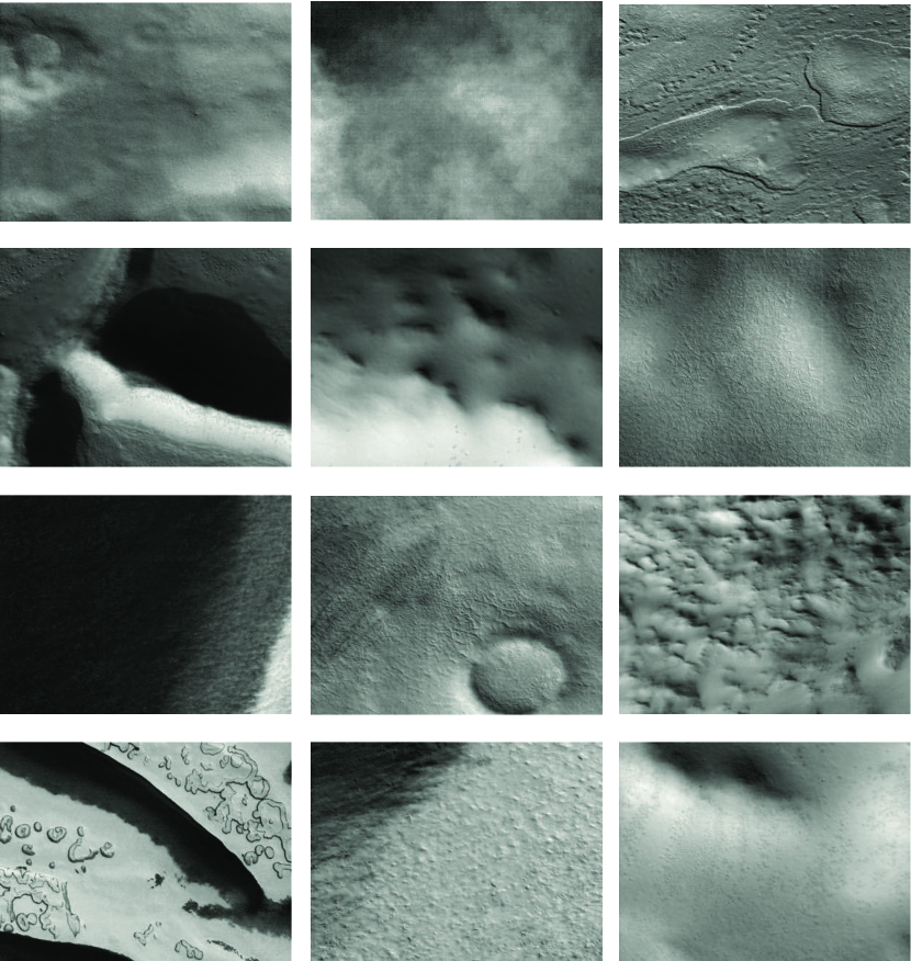
Figure 6: Selection of subjects derived from full frame CTX images shown on the P4T website. Each subject is an 800$\times$600 pixel ($\sim$4.8$\times 3.6$ km) subimage. Starting at top left, Subject IDs (starting with top row, left to right): 489465, 1041974, 489329, 488393, 484326, 1319951, 489919, 1058815, 1040473, 1491825, 1514939, and 1515625. CTX images (starting with top row, left to right): P13$\_$006119$\_$1035, G14$\_$023676$\_$1023,G14$\_$023538$\_$1006, P13$\_$006204$\_$0986, G14$\_$023634$\_$1036,P13$\_$006240$\_$1030, P12$\_$005747$\_$1035, P13$\_$006239$\_$1040,P13$\_$006123$\_$0953, G14$\_$023835$\_$0906, P13$\_$006234$\_$1008,P13$\_$006282$\_$1046

A characteristic sample of P4T subjects is presented in Figure 6. In total 20,122 subjects were generated, and Table LABEL:tab:CTXobs provides a list of the 90 CTX observations and the number of subjects associated with each full frame CTX image. A CTX observation contained a mean of 224 P4T subjects with a minimum of 24 and maximum of 522 subjects. Due to the variable length and width of CTX observations, there are typically small regions on the right and bottom edges of the CTX full frame image that did not make it into a subject image, and thus not searched by P4T. Supplemental Table 1 summarizes the P4T subjects used in this work, including the center latitude, center longitude, and location within the full frame CTX observation.

Table 1: CTX Observations Examined in This Study

CTX image	Latitude	Longitude	$L_{s}$	Observation	$\#$ of
	(degrees)	(degrees)	(degrees)	Time	P4T Subjects
D13$\_$032173$\_$1031$\_$XN$\_$76S227W	-77.02	132.51	331.71	2013-06-07T10:18:40.139	66
D13$\_$032182$\_$1030$\_$XN$\_$77S112W	-77.05	247.78	332.09	2013-06-08T03:08:08.698	183
D13$\_$032278$\_$0991$\_$XN$\_$80S204W	-81.01	155.56	336.15	2013-06-15T14:40:39.298	108
D13$\_$032298$\_$0969$\_$XN$\_$83S028W	-83.18	331.6	336.99	2013-06-17T04:04:24.753	66
D13$\_$032311$\_$0999$\_$XN$\_$80S031W	-80.19	329.04	337.54	2013-06-18T04:23:39.968	304
D13$\_$032352$\_$0985$\_$XN$\_$81S063W	-81.62	296.36	339.25	2013-06-21T09:04:37.135	162
D14$\_$032510$\_$0963$\_$XN$\_$83S054W	-83.71	305.21	345.76	2013-07-03T16:34:14.369	66
D14$\_$032511$\_$0959$\_$XI$\_$84S078W	-84.31	282.04	345.8	2013-07-03T18:26:12.728	48
D14$\_$032517$\_$1000$\_$XN$\_$80S249W	-80.04	110.55	346.04	2013-07-04T05:40:49.097	66
D14$\_$032518$\_$0995$\_$XN$\_$80S281W	-80.51	78.42	346.08	2013-07-04T07:32:06.155	392
D14$\_$032523$\_$0954$\_$XN$\_$84S045W	-84.65	314.82	346.29	2013-07-04T16:52:42.650	66
D14$\_$032530$\_$0975$\_$XN$\_$82S259W	-82.5	100.75	346.57	2013-07-05T05:59:04.972	78
D14$\_$032574$\_$0969$\_$XN$\_$83S005W	-83.17	354.99	348.35	2013-07-08T16:16:02.560	66
D14$\_$032575$\_$0969$\_$XN$\_$83S028W	-83.17	331.6	348.39	2013-07-08T18:08:13.419	66
D14$\_$032593$\_$1037$\_$XN$\_$76S174W	-76.39	185.51	349.12	2013-07-10T03:50:10.687	66
D14$\_$032600$\_$0965$\_$XN$\_$83S357W	-83.56	2.88	349.4	2013-07-10T16:53:27.794	66
D14$\_$032640$\_$1003$\_$XN$\_$79S014W	-79.69	345.3	351.01	2013-07-13T19:42:56.864	87
D14$\_$032656$\_$0959$\_$XI$\_$84S078W	-84.21	281.5	351.65	2013-07-15T01:36:53.707	66
D14$\_$032666$\_$0916$\_$XN$\_$88S350W	-88.51	9.05	352.05	2013-07-15T20:17:50.497	66
D14$\_$032675$\_$0924$\_$XN$\_$87S253W	-87.68	106.58	352.41	2013-07-16T13:08:05.533	66
D14$\_$032682$\_$0925$\_$XN$\_$87S066W	-87.53	293.1	352.69	2013-07-17T02:13:30.246	90
D14$\_$032733$\_$1028$\_$XN$\_$77S036W	-77.24	323.18	354.71	2013-07-21T01:38:54.660	204
D14$\_$032790$\_$0933$\_$XN$\_$86S110W	-86.74	248.82	356.96	2013-07-25T12:11:45.417	24
G13$\_$023338$\_$1043$\_$XI$\_$75S229W	-75.81	131.06	330.91	2011-07-20T00:01:53.559	336
G13$\_$023354$\_$1032$\_$XN$\_$76S301W	-76.82	58.54	331.6	2011-07-21T05:56:38.165	396
G13$\_$023432$\_$1026$\_$XI$\_$77S262W	-77.44	97.75	334.91	2011-07-27T07:49:28.555	294
G13$\_$023452$\_$1049$\_$XN$\_$75S098W	-75.05	261.45	335.75	2011-07-28T21:14:17.312	435
G13$\_$023456$\_$0990$\_$XN$\_$81S204W	-80.98	155.23	335.92	2011-07-29T04:42:00.456	108
G13$\_$023469$\_$1046$\_$XI$\_$75S211W	-75.5	148.2	336.47	2011-07-30T05:02:26.465	210
G14$\_$023496$\_$1047$\_$XI$\_$75S213W	-75.36	147.08	337.6	2011-08-01T07:32:15.443	138
G14$\_$023506$\_$1036$\_$XN$\_$76S132W	-76.42	227.99	338.02	2011-08-02T02:13:28.855	522
G14$\_$023507$\_$1029$\_$XN$\_$77S158W	-77.19	201.15	338.06	2011-08-02T04:06:06.023	120
G14$\_$023524$\_$0999$\_$XN$\_$80S262W	-80.16	97.56	338.77	2011-08-03T11:52:54.656	66
G14$\_$023538$\_$1006$\_$XN$\_$79S285W	-79.48	74.31	339.35	2011-08-04T14:03:39.719	336
G14$\_$023567$\_$1039$\_$XN$\_$76S358W	-76.23	2.04	340.55	2011-08-06T20:18:46.307	438
G14$\_$023577$\_$0999$\_$XN$\_$80S262W	-80.14	97.62	340.97	2011-08-07T15:00:08.617	66
G14$\_$023590$\_$0975$\_$XN$\_$82S259W	-82.54	100.99	341.51	2011-08-08T15:18:11.704	66
G14$\_$023591$\_$0996$\_$XN$\_$80S284W	-80.48	75.43	341.55	2011-08-08T17:10:49.067	132
G14$\_$023616$\_$1004$\_$XN$\_$79S248W	-79.61	111.85	342.58	2011-08-10T15:56:35.480	66
G14$\_$023634$\_$1036$\_$XN$\_$76S027W	-76.44	333.0	343.32	2011-08-12T01:36:48.168	522
G14$\_$023676$\_$1023$\_$XN$\_$77S091W	-77.75	268.09	345.04	2011-08-15T08:09:24.912	294
G14$\_$023687$\_$1031$\_$XN$\_$76S036W	-76.95	323.86	345.49	2011-08-16T04:44:01.680	232
G14$\_$023691$\_$1031$\_$XN$\_$76S143W	-76.98	216.96	345.65	2011-08-16T12:12:04.519	381
G14$\_$023718$\_$1039$\_$XN$\_$76S160W	-76.11	199.16	346.75	2011-08-18T14:42:24.470	348
G14$\_$023728$\_$0958$\_$XI$\_$84S057W	-84.31	302.44	347.15	2011-08-19T09:22:32.460	102
G14$\_$023735$\_$1002$\_$XN$\_$79S262W	-79.88	97.18	347.44	2011-08-19T22:29:22.283	138
G14$\_$023794$\_$0952$\_$XN$\_$84S061W	-84.89	298.47	349.82	2011-08-24T12:48:10.629	66
G14$\_$023807$\_$0886$\_$XN$\_$88S313W	-88.68	47.11	350.34	2011-08-25T13:05:07.603	66
G14$\_$023815$\_$0970$\_$XN$\_$83S282W	-83.05	78.09	350.66	2011-08-26T04:05:02.101	48
G14$\_$023833$\_$0926$\_$XN$\_$87S017W	-87.43	342.35	351.38	2011-08-27T13:43:17.984	66
G14$\_$023835$\_$0906$\_$XN$\_$89S050W	-89.45	310.24	351.46	2011-08-27T17:27:10.913	66
G14$\_$023851$\_$0926$\_$XN$\_$87S180W	-87.41	179.52	352.1	2011-08-28T23:23:15.422	66
G15$\_$023911$\_$1021$\_$XN$\_$77S023W	-77.9	336.45	354.49	2011-09-02T15:38:24.799	66
G15$\_$023927$\_$0932$\_$XI$\_$86S057W	-86.82	302.59	355.12	2011-09-03T21:30:31.425	66
G15$\_$023963$\_$1021$\_$XN$\_$77S006W	-77.91	353.12	356.54	2011-09-06T16:52:57.448	60
P12$\_$005705$\_$1016$\_$XI$\_$78S133W	-78.52	226.28	330.87	2007-10-14T23:21:44.255	294
P12$\_$005747$\_$1035$\_$XI$\_$76S195W	-76.65	164.52	332.66	2007-10-18T05:55:17.203	138
P12$\_$005790$\_$0978$\_$XI$\_$82S284W	-82.26	75.67	334.48	2007-10-21T14:18:20.245	66
P12$\_$005813$\_$1030$\_$XI$\_$77S195W	-77.07	164.97	335.46	2007-10-23T09:20:46.192	66
P12$\_$005839$\_$0994$\_$XI$\_$80S170W	-80.66	189.37	336.55	2007-10-25T09:56:39.216	120
P13$\_$005940$\_$1035$\_$XN$\_$76S064W	-76.51	295.91	340.76	2007-11-02T06:50:28.896	522
P13$\_$005941$\_$0947$\_$XI$\_$85S065W	-85.39	295.0	340.8	2007-11-02T08:39:53.181	408
P13$\_$005953$\_$1020$\_$XN$\_$78S057W	-78.01	302.45	341.3	2007-11-03T07:08:57.500	522
P13$\_$005958$\_$1030$\_$XI$\_$77S195W	-77.02	164.87	341.5	2007-11-03T16:30:56.168	150
P13$\_$006005$\_$0947$\_$XN$\_$85S015W	-85.32	344.59	343.44	2007-11-07T08:22:07.760	408
P13$\_$006112$\_$0852$\_$XN$\_$85S304W	-85.2	55.76	347.8	2007-11-15T16:27:46.904	66
P13$\_$006119$\_$1035$\_$XN$\_$76S271W	-76.52	88.75	348.08	2007-11-16T05:38:06.661	366
P13$\_$006123$\_$0953$\_$XN$\_$84S001W	-84.77	358.59	348.25	2007-11-16T13:04:04.676	522
P13$\_$006146$\_$1045$\_$XN$\_$75S289W	-75.53	70.6	349.17	2007-11-18T08:08:17.767	306
P13$\_$006148$\_$1028$\_$XN$\_$77S342W	-77.25	17.18	349.26	2007-11-18T11:51:51.830	522
P13$\_$006151$\_$0974$\_$XN$\_$82S055W	-82.63	305.13	349.38	2007-11-18T17:27:16.677	252
P13$\_$006161$\_$1030$\_$XN$\_$77S338W	-77.09	22.03	349.78	2007-11-19T12:11:05.625	324
P13$\_$006167$\_$0931$\_$XN$\_$86S092W	-86.96	267.2	350.02	2007-11-19T23:21:18.515	102
P13$\_$006173$\_$0934$\_$XN$\_$86S263W	-86.68	96.7	350.26	2007-11-20T10:34:49.912	66
P13$\_$006174$\_$0958$\_$XN$\_$84S316W	-84.29	43.28	350.3	2007-11-20T12:28:01.397	66
P13$\_$006176$\_$0935$\_$XN$\_$86S350W	-86.51	10.06	350.38	2007-11-20T16:11:29.064	204
P13$\_$006197$\_$0930$\_$XN$\_$87S187W	-87.04	173.3	351.22	2007-11-22T07:27:46.120	150
P13$\_$006199$\_$1040$\_$XN$\_$76S296W	-76.02	63.9	351.3	2007-11-22T11:15:22.194	522
P13$\_$006204$\_$0986$\_$XN$\_$81S065W	-81.45	295.05	351.5	2007-11-22T20:35:13.014	252
P13$\_$006206$\_$1016$\_$XN$\_$78S124W	-78.57	235.47	351.58	2007-11-23T00:20:04.979	504
P13$\_$006207$\_$0956$\_$XN$\_$84S136W	-84.49	223.45	351.62	2007-11-23T02:10:20.857	522
P13$\_$006229$\_$0951$\_$XN$\_$84S014W	-84.97	345.69	352.5	2007-11-24T19:19:03.593	522
P13$\_$006234$\_$1008$\_$XN$\_$79S168W	-79.28	191.3	352.7	2007-11-25T04:42:19.717	306
P13$\_$006239$\_$1040$\_$XN$\_$76S308W	-76.09	51.62	352.9	2007-11-25T14:04:14.736	408
P13$\_$006240$\_$1030$\_$XN$\_$77S335W	-77.04	25.01	352.94	2007-11-25T15:56:00.916	522
P13$\_$006257$\_$1034$\_$XN$\_$76S079W	-77.88	282.15	353.61	2007-11-26T23:43:54.535	264
P13$\_$006271$\_$1010$\_$XN$\_$79S098W	-79.07	261.59	354.17	2007-11-28T01:54:24.701	306
P13$\_$006282$\_$1046$\_$XN$\_$75S043W	-75.47	316.98	354.61	2007-11-28T22:29:37.821	522
P13$\_$006283$\_$1003$\_$XN$\_$79S065W	-79.75	294.76	354.65	2007-11-29T00:20:28.301	522
P13$\_$006290$\_$1017$\_$XN$\_$78S258W	-78.38	101.84	354.92	2007-11-29T13:26:24.488	522

Table 1: The center coordinates for all CTX images searched used in the analysis presented in this paper. The table includes the latitude and longitude, UTC time and date of observation, and number of P4T subjects generated from the observation. We include the full CTX filename here; the first 15 characters are the unique CTX observation identifier.

Figure 3: Top: MOLA shaded relief map [84, 70] with the CTX footprints in magenta. Bottom: The footprints of the surveyed CTX images in magenta overlaid on top of the geologic map from [72]. For both plots, latitude and longitude lines are plotted every 10 degrees. The zero meridian is pointing straight up. A legend for the geologic map is provided in A.

3 Planet Four: Terrains (P4T)

The aim of P4T is to identify features of interest in CTX observations of the South Polar region. For this endeavor we focused on three types of surface features and their distribution on the Martian South Polar region: 1) araneiforms 2) erosional depressions, troughs, mesas, ridges, and quasi-circular pits characteristic of the SPRC which we collectively refer to as ‘Swiss cheese terrain’, and 3) craters. We aim to study the distribution of the araneiforms on the South Polar region and explore their locations compared to the locations of other CO₂ ice sublimation features The crater identifications can aide with the surface age dating of the SPLD, similarly to what has been done for the North Polar region [37]. Examples of each of the three types of surfaces features (taken from the P4T site guide) are shown at the resolution of CTX in Figures 7, 8, and 9.

Several different types of araneiform structures have been identified on the South Polar region [45, 57, 31, 20]. Similar to [20]’s categories identified in HiRISE imaging, we divide araneiform terrain broadly into three araneiform morphologies distinguishable at CTX resolution: ‘baby spiders’, ‘spiders’, and ‘lace terrain’. Spiders are defined as radially converging channels that are often branching and often hosting a visible central pit (see Figure 7). We note for the reader, that any subsequent reference to ‘spiders’ in the text uses this definition. Baby spiders are spiders with ‘short legs’, where a central pit dominates with short or no radial channels (see Figure 7). In the help documentation, we recommend to volunteers that if the channels are shorter than the extent of the central pit, then it is a baby spider. As identification with P4T is through visual inspection, we acknowledge that there is not always a clear dividing line between spiders and baby spiders. The criteria separating the two categories is more qualitative than quantitative. With the resolution of CTX, it is difficult to distinguish patterned ground, formed by the repeating freezing and thawing of soil, from lace araneiforms, formed by the CO₂ jet process. In HiRISE images one can observe the more sinuous nature of the lace araneiforms differentiating these features from polygonal channels, but this is typically not visible in CTX observations. For P4T, we combine lace araneiforms and pattern ground together as one category, referring to them collectively as a ‘channel network’ (see Figure 8). When needed for the channel network regions identified by P4T, we plan to use higher resolution imaging from HiRISE, to distinguish polygonal channels from interconnected araneiforms.

The SPRC’s top surface layers have been categorized into different groups of characteristic smooth-walled features including: troughs, mesas, and quasi-circular pits visible in orbital imagery [e.g 25, 77, 75]. A recent inventory of SPRC surface morphology based on HiRISE and CTX imagery is provided in [77, 75]. The main priority of P4T is to identify new aranieform locations, thus we ask the P4T volunteers to sort araneiforms in more detail by distinguishing araneiforms of different morphology from each other. Given the spatial resolution of CTX and the size of each P4T subject image, we chose to not task P4 volunteers with distinguishing between the different categories established by [77, 75]. For the sublimation features of the SPRC, we combined the morphological categories together into one for P4T which we simply refer to as ‘Swiss cheese terrain’. In the P4T help content (see Figure 8), we describe the Swiss cheese terrain as flat-floored, circular-like depressions and visual examples for P4T show the majority of the different sublimation morphologies visible on the SPRC with CTX. We note for the reader, that any subsequent reference to ‘Swiss cheese terrain’ refers to the combined SPRC sublimation features previously identified.

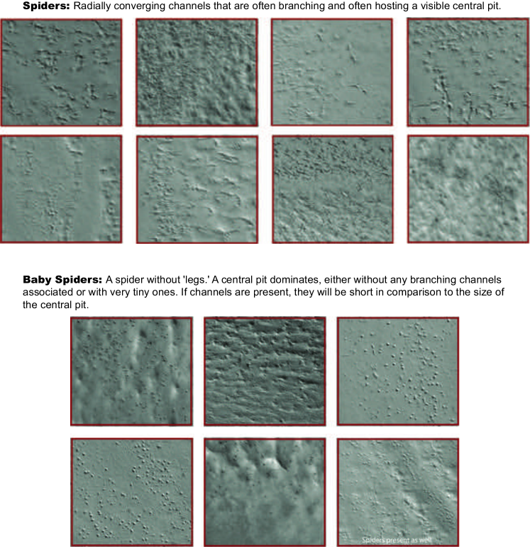
Figure 7: Examples of CTX surface morphologies searched for on P4T continued with the help text provided on the P4T project site guide.

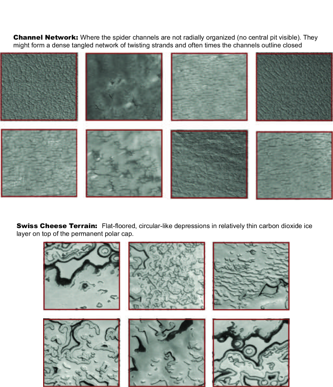
Figure 8: Examples of CTX surface morphologies searched for on P4T continued with the help text provided on the P4T project site guide.

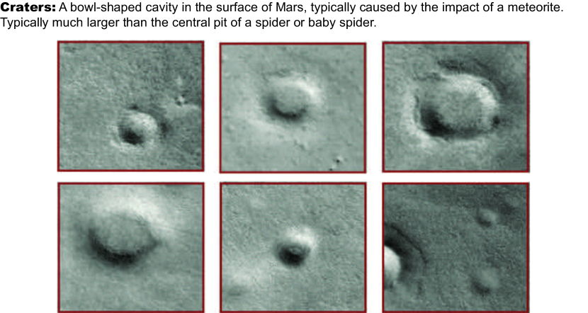
Figure 9: Examples of CTX surface morphologies searched for on P4T continued with the help text provided on the P4T project site guide.

3.1 Web Interface

The Planet Four: Terrains website and online classification interface is built upon the Zooniverse [39, 18] Project Builder platform. The Zooniverse Project Builder platform enables the rapid development of online citizen science projects by providing a set of web-tools for scientists to create and maintain their own citizen science projects. The platform and its Application Program Interface (API) is built upon Amazon Web Services which allows the P4T website to quickly and efficiently scale to handle the load from varying numbers of visitors on the site at the same time; it is capable of supporting tens of thousands of simultaneous users. When a volunteer arrives at the P4T website, the web interface (see Figure 10) displays a selected 800$\times$600 pixel CTX subject. The Zooniverse API pseudo randomly selects a new set of subjects for each classifier upon request, in order to distribute the volunteer effort across the known dataset. In addition, the API algorithm also selects subjects the volunteer has not previously reviewed and that have not been viewed by enough volunteers to mark them as complete. Each subject is typically assessed independently by 20 classifiers before it is retired from review on the P4T website.

Volunteers are tasked with assessing the image and determining what surface features of interest are present in the subject selecting from a choice of: ‘spiders’, ‘baby spiders’, ‘channel network’, ‘Swiss cheese terrain’, ‘craters’ and ‘none of the above’. The volunteer is able to select more than one response that best describes the subject image. In this Paper, a ‘classification’ is defined as the total amount of information collected about one subject by a single volunteer answering the question presented in the P4T classification interface. Help content and example images of each feature/answer choice can be accessed by clicking on the ‘Need some help with this task?’ button. Additional examples and help content are provided on a linked site guide. To minimize external information influencing or biasing a volunteer’s response, no identifying information about the original parent CTX image including the filename or observing circumstances (such as location coordinates, time of day, or L_s) are provided to the volunteer before they submit their classification. Thus the classifier cannot assess whether the image is from a location that previously has been identified as having araneiforms (such as the SPLD) or was previously imaged by HiRISE in previous south polar monitoring observations. To keep the multiple volunteer assessments independent for each subject, the classifier is kept blind to previous people’s responses for the presented subject, and the subject’s internal Zooniverse identifier is hidden from the classification interface.

Once the volunteer selects the categories that best describe the presented subject and hits the ‘Done’ button, the classification is submitted through the Zooniverse API and stored in the Zooniverse PostgreSQL database. The subject identifier, volunteer’s IP (Internet Protocol) address, Zooniverse username if available, timestamp, web browser and operating system information, and user response are recorded. At this point, the volunteer cannot go back and revise their classification. P4T volunteers can classify in two modes: registered with a Zooniverse account or unregistered. The P4T classification interface is presented the same for both registered and non-registered classifiers. The only difference is that non-registered classifiers are reminded from time-to-time to log-in/register for a Zooniverse account. Registered classifications are easily linked by their associated Zooniverse account. For non-registered classifications, a unique identifier is generated and used to link the classifications completed by a given IP address. We note because of the IP tracking, a non-registered classifications from a single IP address may not necessarily equate to a single individual. Additionally, if a volunteer initially classifies non-registered and then logs-in to a Zooniverse account, the previous classifications are not linked with their registered account and remain attributed to an unregistered classifier.

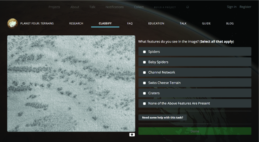
Figure 10: Main classification interface of the P4T website.

3.2 Talk Discussion Tool

After submitting a classification on the P4T website, the classification interface presents the volunteer with two options: ‘Talk’ or ‘Next’. ‘Next’ will load a new subject image in the classification interface. Selecting the ‘Talk’ button instead loads the P4T Talk discussion tool. Talk enables volunteers to further explore the P4T dataset beyond the main tasks and aims of the classification interface. The discussion tool hosts message boards that support interactions with the science team and others in the P4T volunteer community. Each subject has a dedicated page on Talk where a registered volunteer can initiate a new discussion or add commentary to an on-going discussion about the subject. Volunteers can also associate the subject with searchable Twitter-like hashtags and link multiple subjects together into groups. Reading previously posted commentary on Talk might bias a volunteer’s assessment in the classification interface. To maintain the independence of the classifications, the Zooniverse identifier for the subject is not presented in the classification interface and the direct link for the Talk subject page is only revealed after a volunteer submits their classification to the Zooniverse database. For this work, we focus primarily on the results from the main classification interface.

3.3 Site History and Statistics

The 20,122 subjects derived from the 90 CTX full frame images used in this study were classified by 6,309 registered Zooniverse users and 8,513 non-logged-in sessions (tracked by IP address). The classifications were collected from June 24, 2015 to August 10, 2016. We plot the distribution of registered volunteers and non-logged-in sessions as a function of number of classifications in Figure 11. Registered volunteers classified a mean of 61 subjects with a median of 14. Non-logged-in sessions classified an average of 19 and median of 5 subjects. 20$\%$ of registered volunteers classified more than 50 subjects, while only 3$\%$ of non-logged-in sessions classified more than 50 subjects.

We plot the distribution of classifications per subject in Figure 12. The majority of the subjects received 20 classifications or more. Due to a bug in the backend of the Zooniverse platform, some volunteers were shown the same subject to classify twice or more. To ensure the assessments for each subject remain independent, we filter the classification database and remove any duplicate classifications keeping the first response from the registered username or IP address in the case of non-logged classifications. For all the values reported in this Paper, we use the filtered classifications. In some cases, this will leave a subject with less than 20 independent assessments, but the impact is negligible with only 7$\%$ of the subjects in this study having less than 20 unique classifications and 0.07$\%$ with less than 17 unique classifications. We also note that due to a glitch in the backend of the Zooniverse platform a portion of P4T subjects were not retired after 20 classifications. 8$\%$ of the subjects in this study received more than 25 independent assessments, with only 3$\%$ of the subjects receiving more than 50 classifications.

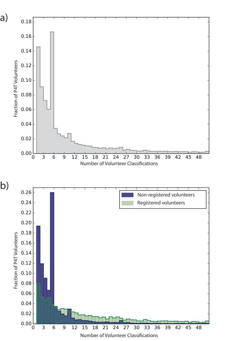
Figure 11: Distribution of P4T volunteer classifications used in this work. Figure a shows the combined distribution of both logged-in and non-logged in sessions. Figure b shows the volunteer classification count individually for registered and non-logged volunteers. Both distributions use a bin size of 1, the distributions plotted are cut off beyond 50 classifications.

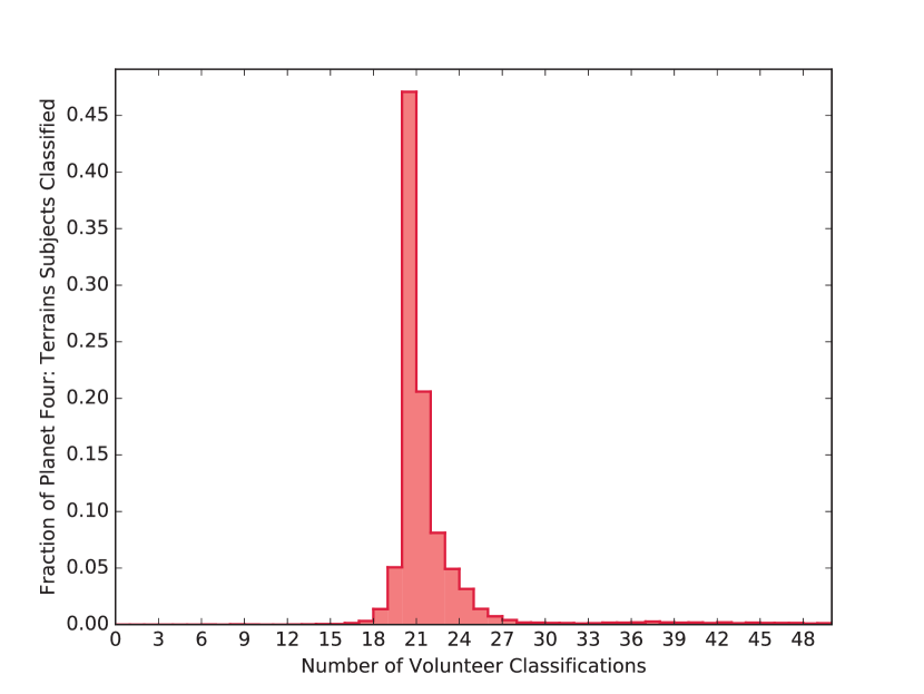
Figure 12: Histogram of the number of P4T classifications per subject used in this work. The distribution was generated with a bin size of 1 and for clarity the plot is cut off beyond 50 classifications.

4 Data Analysis

For this work, we focus solely on the P4T identification of spiders and Swiss cheese terrain. We refer the reader to Section 3 for the specific definitions of spiders and Swiss cheese terrain we use in this analysis. We combine the multiple volunteer classifications of a given subject together, examining the number of volunteers who selected the ‘spiders’ or ‘Swiss cheese terrain’ buttons for each subject in order to identify spiders and Swiss cheese terrain present in the P4T data. Some volunteers may be better at spotting these features than others. Rather than treat all volunteer assessments equality, we apply a user weighting scheme that enables us to pay more attention to those volunteers who are better at identifying spiders or Swiss cheese terrain and also reduce the influence of potentially unreliable classifiers, such as those who did not engage in or understand the task. We then apply these weights when combining the volunteer assessments for spiders or Swiss cheese to determine how likely a P4T image is to have these features of interest present.

4.1 User Weighting Scheme

We use a modified version of the iterative user weighting schemes developed by [40] and [39] for the visual morphological classifications of galaxies in the Galaxy Zoo project and by [69] for the visual identification of planet transits in NASA Kepler data in the Planet Hunters project. The weighting scheme evaluates the ability of each classifier and assigns a weight based on their tendency to agree with the majority opinion, distinguishing those volunteers who are better at spotting Swiss cheese or spiders in order to pay attention to their responses more than others when identifying which subjects have these features present.

We define a ‘user’ for our case as either a volunteer with a registered Zooniverse account or the collective behavior of non-logged-in sessions with a unique-IP address. A unique non-logged-in IP address may not necessarily by a single individual (see 3.1), but for the weighting scheme we link the classifications together and determine a single weight. If a user excels at identifying spiders, it does not necessarily mean they would be as good as identifying Swiss cheese terrain in the P4T data. We therefore treat the identification of spiders and Swiss cheese terrain independently as two separate classes of responses, and determine separate user weights for each class. For the analysis presented here, the volunteer classifications are effectively divided into two responses per class: ‘found’ and ‘not found’. For spider identification this breaks down into ‘spiders found’ if the volunteer selected the ‘spider’ button while classifying the subject and ‘no spiders found’ if the volunteer did not select the ‘spiders’ button. For this analysis, if a volunteer clicked on the ‘baby spiders’ or ‘channel network’ buttons without also clicking on the ’spiders’ button, this would count as a ’no spiders found’ response for the subject image. We do the same thing with the responses for Swiss cheese terrain, with a vote of ‘Swiss cheese found’ if the ’Swiss cheese terrain’ button was selected when the subject image was reviewed or ‘no Swiss cheese found’ if volunteer didn’t mark the image as having Swiss cheese terrain.

Each user $j$ is assigned two weights, one for each class: $w_{j}(\rm spider)$ and $w_{j}(\rm Swiss)$. Initially, all users start out with each of those weights equal to 1. Then for each P4T subject i scores for spiders, $s_{i}(\rm spider)$, and Swiss cheese pits, $s_{i}(\rm Swiss)$, are calculated. We define these scores per subject as follows:

$$s_{i}(\rm spider) = \frac{1}{S_{i}}\displaystyle\sum_{k}w_{k}(\rm spiders)\qquad k\textrm{=users who selected `spider' for subject \emph{i}}$$ (1)

$$s_{i}(\rm Swiss) = \frac{1}{C_{i}}\displaystyle\sum_{m}w_{m}(\rm Swiss)\qquad m\textrm{=users who selected `Swiss cheese' for subject \emph{i}}$$ (2)

where $S_{i}$ and $C_{i}$ are the sum of the respective user weights for all the users who classified subject i:

$$S_{i} = \displaystyle\sum_{k=j}w_{k}(\rm spiders)\qquad$$ (4)

$$C_{i} = \displaystyle\sum_{m=j}w_{m}(\rm Swiss)\qquad$$ (5)

$$j =$$ all users who classified subject i

Subject scores vary between the values of 0 and 1, inclusive. A subject score of 1 is assigned if all volunteers who classified the subject agree and identified the same features of interest in the subject image.

Once the subject scores $s_{i}(\rm spider)$ and $s_{i}(\rm Swiss)$ are calculated, we next assign new user weights for each user $j$ by the prescription below:

$$w_{j}(spiders) = \left\{\begin{array}[]{ll}\displaystyle{\frac{A}{N_{j}}\sum_{i=p}s_{i}(\rm spider)+\frac{A}{N_{j}}\sum_{i=q}[1-s_{i}(\rm spider)]}&\textrm{if $N_{j}>1$}\\ 1&\textrm{if $N_{j}=1$}\end{array}\right.$$ (8)

$$p =$$ subjects volunteer classified as ‘spiders found’

$$q =$$ subjects volunteer classified as ‘spiders not found’

$$w_{j}(Swiss) = \left\{\begin{array}[]{ll}\displaystyle\frac{B}{N_{j}}\sum_{i=t}s_{i}(\rm Swiss)+\frac{B}{N_{j}}\sum_{i=u}[1-s_{i}(\rm Swiss)]&\textrm{if $N_{j}>1$}\\ 1&\textrm{if $N_{j}=1$}\end{array}\right.$$ (11)

$$t =$$ subjects volunteer classified as ‘Swiss cheese found’

$$u =$$ subjects volunteer classified as ‘Swiss cheese not found’

where $N_{j}$ is the number of subjects classified by user j. The scaling factors $A$ and $B$ are chosen to be such that the median user weight for volunteers who classify more than one subject will be 1. We only adjust the weights of those volunteers who have classified more than one subject, which constitutes 85$\%$ of P4T users. With a single classification there is not much information to use to evaluate a volunteer’s ability to discern spiders and Swiss cheese terrain. Thus for those users who have classified a single subject, we choose to keep the user weights static at a value of 1, where the median of the adjusted weights will lie. A volunteer who has classified more than one subject is upweighted strongly when they agree with the majority weighted vote and down weighted more harshly when their response is at odds with the majority of the volunteers who reviewed the subject image.

After the user weights are first adjusted, the subject scores in each class, $s_{i}(\rm spider)$ and $s_{i}(\rm Swiss)$, are recalculated using the updated user weights with Equations 1 and 2. Then new user weights are assigned with Equations 6 and 7. The process is iterated until convergence is achieved, when the median absolute difference between the old and updated user weights is less than or equal to 1x10^-4, in this case after four iterations for both spiders and Swiss cheese. We plot the distribution of user weights for spiders in Figure 13 and for Swiss cheese terrain in Figure 14. With this scheme, a user weight can never be zero. For $w_{j}(\rm spider)$, 91$\%$ of users have weights greater than 0.8 and 43$\%$ of user weights are greater than 1. For $w_{j}(\rm Swiss)$, 89$\%$ of users have weights greater than 0.8 and 43$\%$ of user weights are greater than 1.

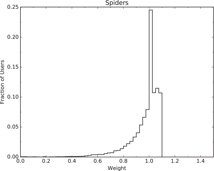
Figure 13: Histogram of spider user weights, $w(\rm spider)$, plotted with a bin size of 0.025

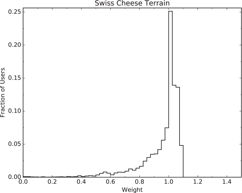
Figure 14: Histogram of Swiss Cheese user weights, $w(\rm Swiss)$, plotted with a bin size of 0.025

4.2 Combining User Classifications and Gold Standard Data

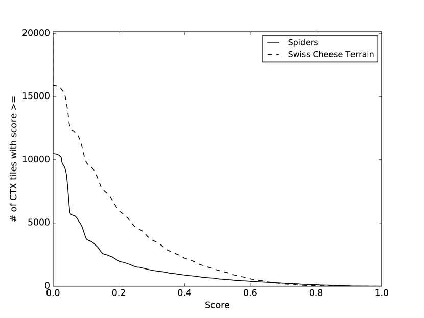
Figure 15: Cumulative distribution of spider and Swiss cheese terrain scores ($s_{i}(\rm spider)$ and $s_{i}(\rm spider)$) for P4T subjects.

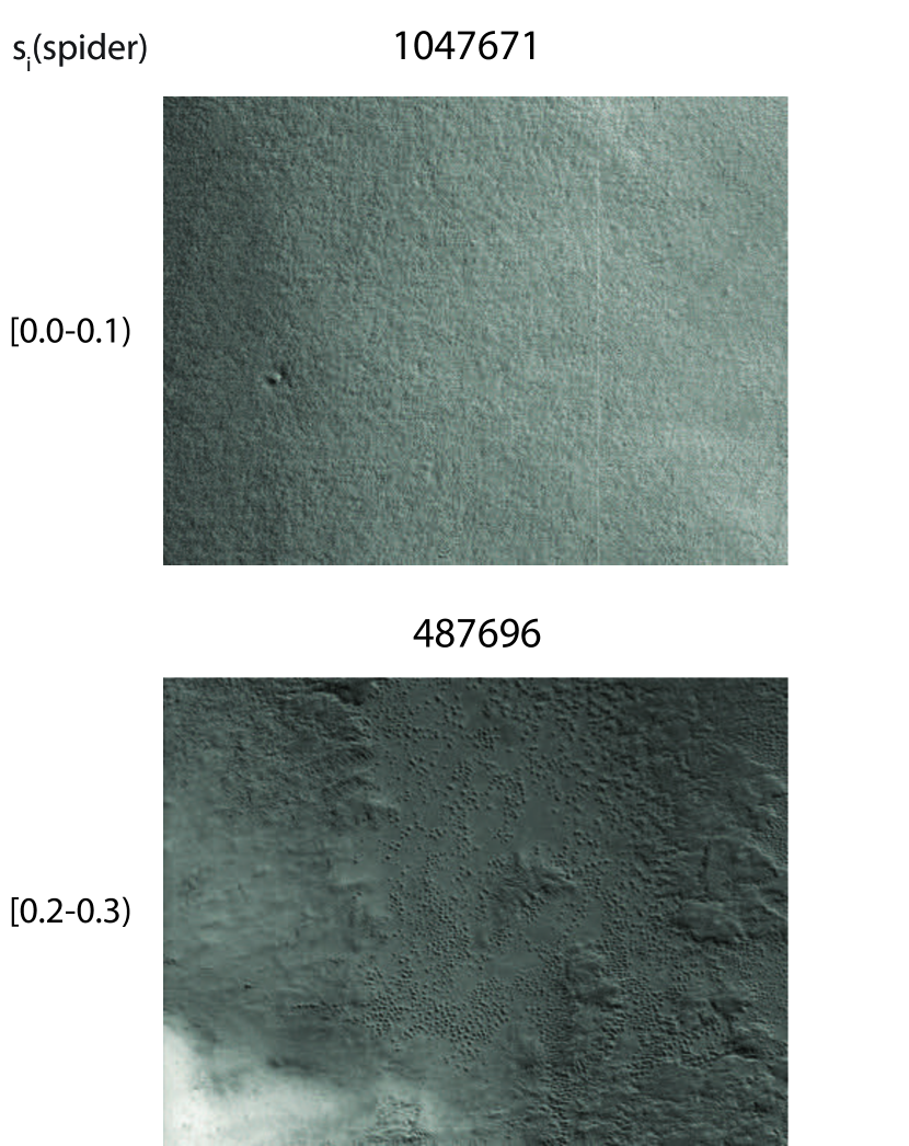
Figure 16: Randomly selected sample of subjects per spider score ($s_{i}(\rm spider)$) binned with bin size of 0.1. CTX images D14$\_$032593$\_$1037 (top) and P13$\_$005953$\_$1020 (bottom). Each P4T subject image is $\sim$4.8$\times 3.6$ km.

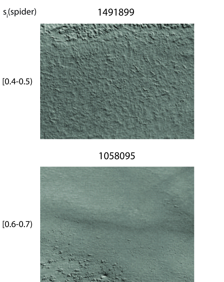
Figure 17: Randomly selected sample of subjects per spider score ($s_{i}(\rm spider)$) binned with bin size of 0.1 continued. CTX images: G14$\_$023524$\_$0999 (top) and P13$\_$006151$\_$0974(bottom). Each P4T subject image is $\sim$4.8$\times 3.6$ km.

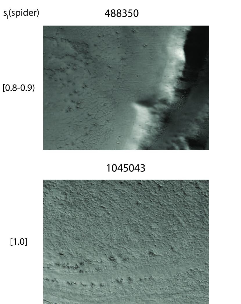
Figure 18: Randomly selected sample of subjects per spider score ($s_{i}(\rm spider)$) binned with bin size of 0.1 continued. CTX images: P13$\_$006204$\_$0986 (top) and P13$\_$006151$\_$0974 (bottom). Each P4T subject image is $\sim$4.8$\times 3.6$ km.

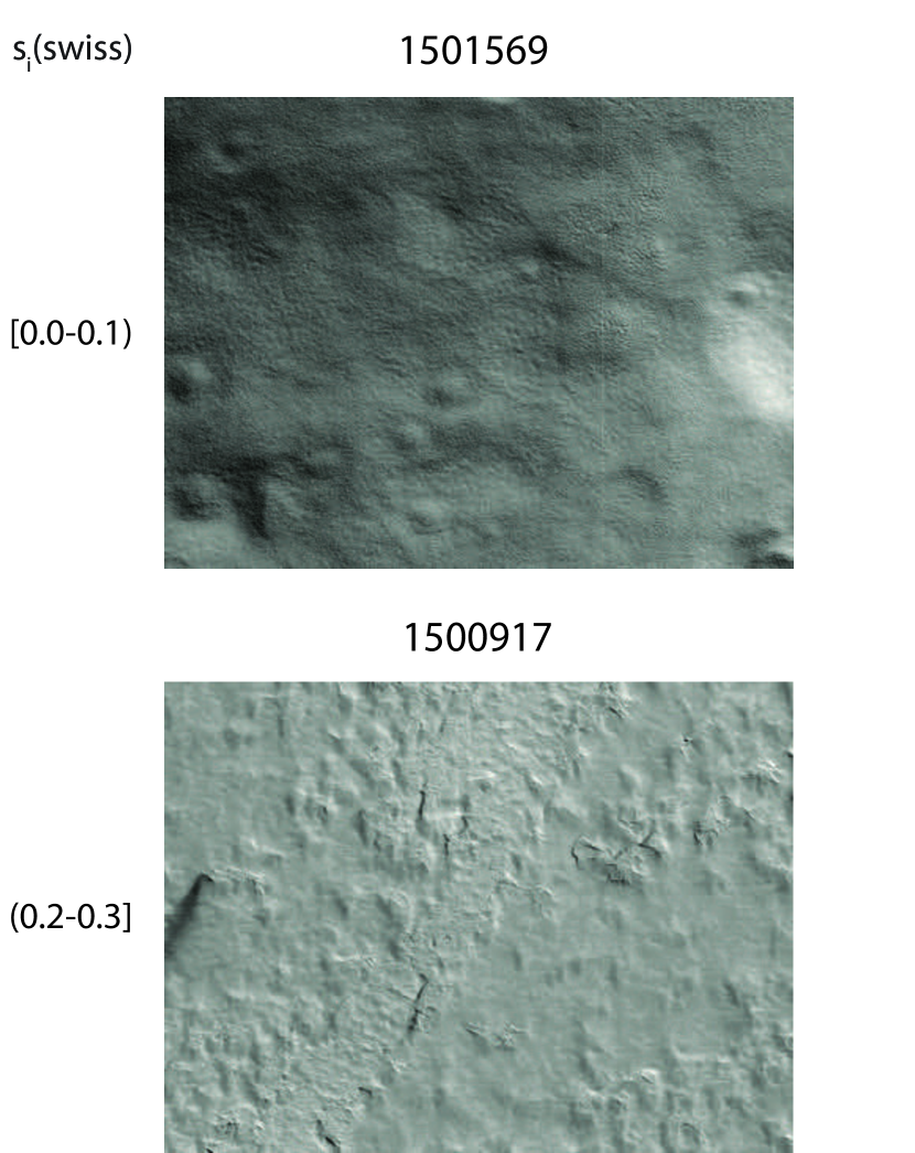
Figure 19: Randomly selected sample of subjects per Swiss cheese score ($s_{i}(\rm Swiss)$) binned with bin size of 0.1. CTX images: P13$\_$006199$\_$1040 (top) and D13$\_$032311$\_$0999 (bottom). Each P4T subject image is $\sim$4.8$\times 3.6$ km.

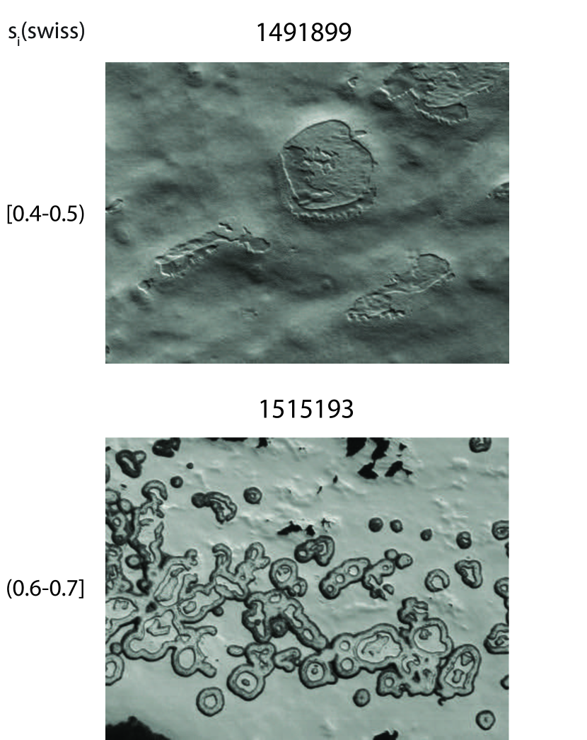
Figure 20: Randomly selected sample of subjects per Swiss cheese score ($s_{i}(\rm Swiss)$) binned with bin size of 0.1 continued. CTX images: G14$\_$023524$\_$0999 (top) and P13$\_$006234$\_$1008(bottom). Each P4T subject image is $\sim$4.8$\times 3.6$ km.

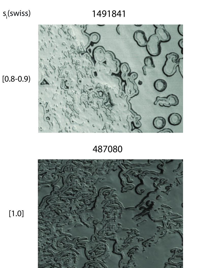
Figure 21: Randomly selected sample of subjects per Swiss cheese score ($s_{i}(\rm Swiss)$) binned with bin size of 0.1 continued. CTX images: G14$\_$023835$\_$0906(top) and P13$\_$006229$\_$0951 (bottom). Each P4T subject image is $\sim$4.8$\times 3.6$ km.

We then use the final subject scores, $s_{i}(\rm spider)$ and $s_{i}(\rm Swiss)$, to identify the locations of spiders and Swiss cheese terrain in the surveyed CTX images. Figure 15 plots the cumulative distribution for the final calculated scores. Table 2 reports the binned distribution in subject scores, and Table 4.3 provides the final score values for each subject used in this study. Figures 16-18 contain a representative sample of subjects for $s_{i}(\rm spider)$ randomly selected in bins of 0.1. Figures 19-21 show the same for $s_{i}(\rm Swiss)$. It is readily apparent the closer the subject score is to 1, the more consensus amongst the weighted user vote and thus a higher likelihood of the features of interest (spiders or Swiss cheese terrain) being present in a given subject image. Of the 20,122 subjects classified by P4T volunteers, 3$\%$ (591) have $s_{i}(\rm spider)$ $>$ 0.5 and 9$\%$ (1767) have $s_{i}(\rm Swiss)$ $>$ 0.5.

We set a detection threshold for $s_{i}(\rm spider)$ and $s_{i}(\rm Swiss)$ above which we define a clean sample of subjects identified as having spiders or Swiss cheese terrain present. We set this value such that the number of false positives is sufficiently small while retaining the largest number of true identifications. We determine this detection limit based on the expert assessment by the P4T science team for a small fraction of the subject data used in this study. A similar validation process has been applied to crowd-sourced crater counting [66, 8]. A subset comprised of 1,009 subjects (505 for Swiss cheese terrain identification and 504 for spider identification), corresponding in total to 5$\%$ of the total subjects reviewed by volunteers, were used to create the gold standard dataset. The subjects were divided into ten bins based on $s_{i}(\rm spider)$ and $s_{i}(\rm Swiss)$. The gold standard subjects were randomly selected from these bins in order to find the subject score where false positives begin to overwhelm positive identifications of spiders and Swiss cheese terrain. Table 2 details the number of subjects per $s_{i}(\rm spider)$ and $s_{i}(\rm Swiss)$ bins randomly selected for the gold standard review. The P4T subject ids used in the expert gold standard review are provided in Supplemental Tables 2 and 3.

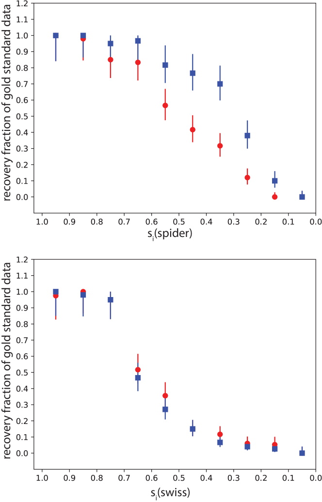
Figure 22: Detection efficiency/recovery rate of subjects with spider and Swiss cheese features per subject score ($s_{i}(\rm spider)$ and $s_{i}(\rm Swiss)$) in the gold standard dataset bin size of 0.1. The assessments from the two expert reviewers, MES and GP) are plotted separately as red circles and blue squares respectively. Error bars represent the Poissonian 1-$\sigma$ uncertainty.

Two members of the science team (MES and GP) each independently reviewed the gold standard subjects using the same web interface on the P4T website as used by the volunteers. The gold standard assessments are available in Supplemental Table 4. Figure 22 plots for the gold standard dataset, the fraction of positive identification of spider and Swiss cheese detections as a function of score for each expert reviewer. The error bars represent the Poissonian 68$\%$ confidence limit on the positive identifications in each bin, as prescribed by [35]. There is strong agreement in expert assessments for Swiss cheese terrain, but less agreement for spider assessments. This may be due to differing levels of difficulty between the two identification tasks.

4.3 Clean Spider and Swiss Cheese Terrain Sample

We set our detection threshold for $s_{i}(\rm spider)$ and $s_{i}(\rm Swiss)$ at the score bin where 20$\%$ of the gold standard data subjects reviewed are false positives as deemed by both expert reviewers. Therefore, we select our ‘clean’ sample of spider detections as subjects with $s_{i}(\rm spider)\geq 0.6$, and our ‘clean’ Swiss cheese sample is comprised of subjects with $s_{i}(\rm Swiss)\geq 0.7$. Applying these cuts, 390 (1.9$\%$) of the P4T subjects have $s_{i}(\rm spider)\geq$ 0.6, and 1,537 (7.6$\%$) have $s_{i}(\rm Swiss)\geq 0.7$. We use the clean samples in the rest of our analysis.

The clean spider and clean swiss cheese identifications do not represent a complete sample in our search region. Instead these are high confidence identifications where false positives in the sample are minimized. Thus a location within the searched CTX images that is not part of our clean samples, may still have spider-shaped araneiforms or Swiss cheese terrain present that are not easily identified by P4T which includes cases where the surface may not be as visible in the CTX image (see Section 2). Thus our analysis only focuses on what we can glean from a sample of confident identifications with approximately less than 20$\%$ false positives. We provide a catalog of the subjects and associated properties that comprise the clean spider and Swiss cheese samples in Tables 4.3 and 4.3 respectively.

[h] P4T Subject Information and $s_{i}{(\textrm{s}pider)}$ and $s_{i}{(\textrm{S}wiss)}$ Scores Center Center Subject ID $s_{i}{(\textrm{s}pider)}$ $s_{i}{(\textrm{S}wiss)}$ Parent CTX Image Latitude Longitude CTX X^∗ CTX Y^∗ (degrees) (degrees) position position 83672 0.025 0.000 G14$\_$023507$\_$1029$\_$XN$\_$77S158W -77.80 200.96 400 300 483673 0.074 0.000 G14$\_$023507$\_$1029$\_$XN$\_$77S158W -77.74 200.90 400 900 483674 0.000 0.000 G14$\_$023507$\_$1029$\_$XN$\_$77S158W -77.68 200.84 400 1500 483675 0.122 0.016 G14$\_$023507$\_$1029$\_$XN$\_$77S158W -77.62 200.78 400 2100 483676 0.167 0.000 G14$\_$023507$\_$1029$\_$XN$\_$77S158W -77.56 200.72 400 2700 483677 0.131 0.000 G14$\_$023507$\_$1029$\_$XN$\_$77S158W -77.50 200.66 400 3300 483678 0.237 0.015 G14$\_$023507$\_$1029$\_$XN$\_$77S158W -77.45 200.60 400 3900 483679 0.066 0.057 G14$\_$023507$\_$1029$\_$XN$\_$77S158W -77.39 200.54 400 4500 483680 0.069 0.015 G14$\_$023507$\_$1029$\_$XN$\_$77S158W -77.33 200.48 400 5100

• CTX X and CTX Y are the pixel location of the subject’s center in the full frame CTX ISIS generated cube.

• This table in its entirety can be found in the online Supplemental and at https://www.zooniverse.org/projects/mschwamb/planet-four-terrains/about/results A portion is shown here for guidance regarding its form and content. We include the full CTX filename here; the first 15 characters are the unique CTX observation identifier.

Table 2: Distribution of P4T Scores for All Subjects and Subjects Used in the Gold Standard Review

bins	$s_{i}{(\textrm{s}pider)}$	$s_{i}{(\textrm{S}wiss)}$	gold spider	gold Swiss
0 $\leq s_{i}{()}<$ 0.1	16301	15885	30	28
0.1 $\leq s_{i}{()}<$ 0.2	1846	1533	40	38
0.2 $\leq s_{i}{()}<$ 0.3	713	483	50	50
0.3 $\leq s_{i}{()}<$ 0.4	383	290	60	60
0.4 $\leq s_{i}{()}<$ 0.5	288	164	60	60
0.5 $\leq s_{i}{()}<$ 0.6	201	135	60	59
0.6 $\leq s_{i}{()}<$ 0.7	150	95	60	60
0.7 $\leq s_{i}{()}<$ 0.8	117	114	60	60
0.8 $\leq s_{i}{()}<$ 0.9	88	353	49	50
0.9 $\leq s_{i}{()}\leq$ 1.0	35	1070	35	40
Total	20122	20122	504	510

[h] Clean Spider Sample Subject ID $s_{i}{(\textrm{s}pider)}$ Parent CTX lmage Center Latitude Center Longitude (degrees) (degrees) 489994 1.000 P12$\_$005747$\_$1035$\_$XI$\_$76S195W -76.76 165.32 491505 1.000 D14$\_$032675$\_$0924$\_$XN$\_$87S253W -87.55 110.18 1045043 1.000 P13$\_$006151$\_$0974$\_$XN$\_$82S055W -82.13 303.34 1320810 1.000 P12$\_$005839$\_$0994$\_$XI$\_$80S170W -81.10 189.69 1510306 0.953 G13$\_$023338$\_$1043$\_$XI$\_$75S229W -75.34 131.48 491434 0.953 P13$\_$006173$\_$0934$\_$XN$\_$86S263W -86.73 100.61 491859 0.951 P13$\_$006148$\_$1028$\_$XN$\_$77S342W -79.08 19.48 1491749 0.951 P13$\_$006197$\_$0930$\_$XN$\_$87S187W -86.91 172.28 1058665 0.951 D14$\_$032593$\_$1037$\_$XN$\_$76S174W -76.20 185.99

• This table in its entirety can be found in the online Supplemental and at https://www.zooniverse.org/projects/mschwamb/planet-four-terrains/about/results A portion is shown here for guidance regarding its form and content. We include the full CTX filename here; the first 15 characters are the unique CTX observation identifier.

Clean Swiss Cheese Terrain Sample Subject ID $s_{i}{(\textrm{S}wiss)}$ Parent CTX Image Center Latitude Center Longitude (degrees) (degrees) 1320528 1.000 P13$\_$006005$\_$0947$\_$XN$\_$85S015W -86.32 355.10 1320615 1.000 P13$\_$006005$\_$0947$\_$XN$\_$85S015W -85.39 345.54 1320728 1.000 P13$\_$006005$\_$0947$\_$XN$\_$85S015W -86.34 359.96 1491818 1.000 G14$\_$023835$\_$0906$\_$XN$\_$89S050W -89.36 342.33 1491849 1.000 G14$\_$023835$\_$0906$\_$XN$\_$89S050W -89.14 300.68 1040008 1.000 G14$\_$023833$\_$0926$\_$XN$\_$87S017W -87.75 346.66 1040047 1.000 G14$\_$023833$\_$0926$\_$XN$\_$87S017W -87.38 342.37 1040089 1.000 P13$\_$006123$\_$0953$\_$XN$\_$84S001W -86.26 9.46 1040272 1.000 P13$\_$006123$\_$0953$\_$XN$\_$84S001W -85.75 5.97

• This table in its entirety can be found in the online Supplemental and at https://www.zooniverse.org/projects/mschwamb/planet-four-terrains/about/results A portion is shown here for guidance regarding its form and content. We include the full CTX filename here; the first 15 characters are the unique CTX observation identifier.

5 Spider Distribution

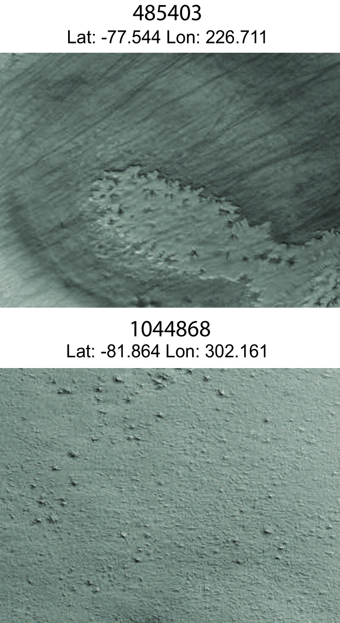
Figure 25: Representative sample of each of the regions identified in the clean spider sample as outside of the SPLD unit. P4T subjects derived from CTX images P13$\_$006151$\_$0974 and D14$\_$032733$\_$1028.Each P4T subject image is $\sim$4.8$\times 3.6$ km.

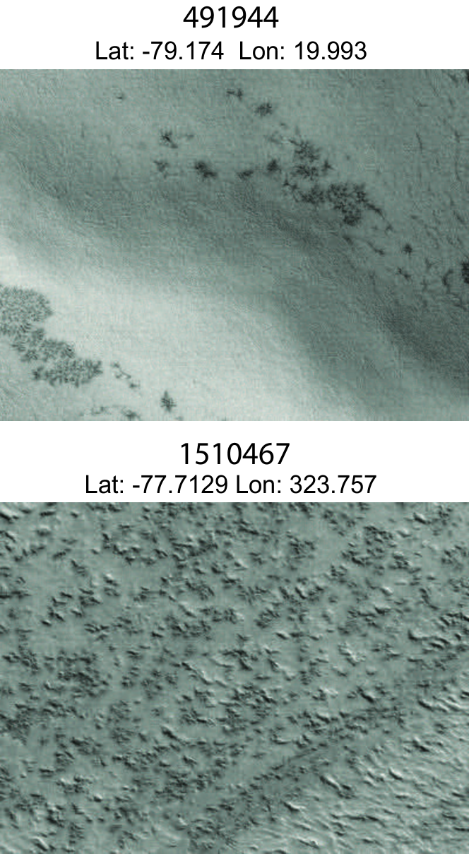
Figure 26: Representative sample of each of the regions identified in the clean spider sample as outside of the SPLD unit, continued. P4T subjects derived from CTX images G14$\_$023506$\_$1036 and P13$\_$006151$\_$0974.Each P4T subject image is $\sim$4.8$\times 3.6$ km.

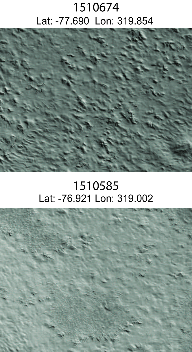
Figure 27: Representative sample of each of the regions identified in the clean spider sample as outside of the SPLD unit, continued. P4T subjects derived from CTX images P13$\_$006148$\_$1028 and P13$\_$006283$\_$1003. Each P4T subject image is $\sim$4.8$\times 3.6$ km.

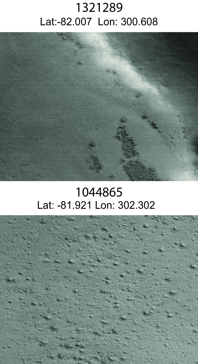
Figure 28: Representative sample of each of the regions identified in the clean spider sample as outside of the SPLD unit, continued. P4T subjects derived from CTX images P13$\_$006151$\_$0974 and P13$\_$006282$\_$1046. Each P4T subject image is $\sim$4.8$\times 3.6$ km.

Our clean spider sample is comprised of 390 subjects, and their locations are plotted in Figure 23 overlaid on a MOLA elevation map [84, 70] and the geologic map from [72]. Using MOC Narrow Angle observations, [57] previously mapped the distribution of spiders in the South Polar region. They found a correlation between areneiforms and CO₂ slab ice, which is thought to be required for the CO₂ jet process. Additionally, [57] found that areneiforms were restricted to the SPLD. All but one grouping of their araneiform regions found in the [57] study were located within the definition of the SPLD at the time. The outlier region (located at approximately latitude=-82^∘, longitude=35^∘) has similar surface characteristics to the SPLD, and the more modern [72] definition does include this location within the SPLD. There is no published table of [57]’s positive identifications, only the plotted distribution in Figure 2 from their paper. In order to compare our clean spider sample to that observed by [57], in Figure 24 we overlay our clean spider distribution on top of [57]’s Figure 2a. Like [57], we find the spiders are concentrated on the SPLD with $75\%$ of the clean sample located on the [72] defined SPLD, but we also have 96 identifications located outside of the SPLD. We list these locations and subject details in Table LABEL:tab:spiders_off_spld and display a set of representative subject images of these regions in Figures 25-31. With the gold standard classifications providing a $\sim$20$\%$ value for the false positive rate, we are confident that the majority of the subjects identified in the clean sample as outside of the SPLD are valid. In order to verify the detection of araneiform features outside of the SPLD, we have also obtained high resolution imaging with HiRISE. We present those observations in Section 7. With this discovery, we find for the first time that there are surfaces other than the SPLD on the Martian South Polar region that are conducive to the growth of araneiforms.

We further investigated why the araneiform features outside of the SPLD in our clean spider sample were not found by [57]. The MOC NA camera has better resolution ($\sim$1-2 m per pixel) but less coverage per image than CTX does. One would have expected these features to be more clearly visible if present in the MOC NA images surveyed by [57]. Examining the coverage of the MOC NA observations used by [57], we find that the locations listed in Table LABEL:tab:spiders_off_spld are either outside the search area or in regions with less than $20\%$ coverage. Thus, the likely reason why these araneiforms features were first identified by P4T is that these areas were covered in the CTX observations and not in the [57] reviewed observations. Bolstering this argument is the araneiform identifications from [61] which surveyed MOC NA observations from September 1997 to March 2004, including reviewing newer observations than what was available to [57]. [61] did not compare their araneiform identifications to the outline of the SPLD or the locations of other geologic units. Although [61] do not resolve araneiform identifications to subimage positions, comparing their distribution, we find that there are several identifications outside of the SPLD (E0701468, R0902433, R0902028, R0901662, R0800241, R0904104, R0801805, R0903024, R0903639, R0701390, R0801195, M1101070, R0601143, R0903607, R0901019, R0601842, R0902403, R0903025, M1102723, M0905981, M1103774,M1000442, M1301816, and M0900454). With a visual inspection, we find many of these off SPLD MOC observations identified as containing araneiforms by [61] are heavily covered with dark seasonal fans, making it more difficult for a positive identification. In our P4T search, the majority of the CTX observations are ice free off the SPRC, allowing for clearer identification of spiders and other types of araneiforms.

Table 3: Clean Spider Sample Outside of the SPLD

Subject ID	Center Latitude	Center Longitude
	(degrees)	(degrees)
1044650	-82.4	303.03
1044654	-82.34	302.88
1044658	-82.29	302.73
1044835	-82.27	303.19
1045035	-82.24	303.64
1044662	-82.23	302.58
1058053	-82.22	304.11
1044841	-82.21	303.03
1058095	-82.20	304.56
1058054	-82.16	303.95
1058096	-82.14	304.40
1045043	-82.13	303.34
1058055	-82.11	303.79
1044851	-82.09	302.73
1058139	-82.06	304.69
1321289	-82.01	300.61
1058140	-82.00	304.53
1044676	-82.00	302.00
1044860	-81.98	302.44
1058099	-81.97	303.93
1045055	-81.96	302.89
1321290	-81.95	300.45
1058141	-81.94	304.37
1044681	-81.94	301.86
1058058	-81.93	303.34
1044865	-81.92	302.30
1058100	-81.91	303.78
1045059	-81.9 0	302.75
1321291	-81.89	300.29
1044687	-81.88	301.72
1058059	-81.88	303.19
1044868	-81.86	302.16
1058101	-81.85	303.63
1044690	-81.83	301.59
1044697	-81.77	301.45
1044878	-81.75	301.89
1321091	-81.33	297.46
1321181	-81.14	297.50
487949	-80.42	306.11
488331	-80.41	292.65
487950	-80.36	306.00
487697	-79.95	304.11
487698	-79.89	304.02
487785	-79.87	304.38
491934	-79.76	20.89
491935	-79.70	20.79
491675	-79.7 0	19.62
491849	-79.66	20.34
491850	-79.6	20.25
489241	-79.53	74.18
491679	-79.46	19.28
491766	-79.44	19.64
491594	-79.36	18.77
491768	-79.33	19.47
491595	-79.3	18.69
491682	-79.29	19.04
492029	-79.27	20.51
491769	-79.27	19.38
491856	-79.25	19.73
491596	-79.24	18.61
491943	-79.23	20.08
491683	-79.23	18.96
492030	-79.22	20.42
491857	-79.19	19.65
491944	-79.18	19.99
492031	-79.16	20.33
491771	-79.15	19.22
491858	-79.13	19.57
491945	-79.12	19.91
492032	-79.10	20.25
491859	-79.08	19.48
491946	-79.06	19.82
491947	-79.00	19.74
492034	-78.98	20.08
491040	-78.98	230.66
491774	-78.97	18.98
491127	-78.96	231.00
491948	-78.94	19.66
491863	-78.84	19.16
485155	-77.77	225.05
1510467	-77.71	323.76
485156	-77.71	225.02
1510416	-77.7	324.06
1510674	-77.69	319.85
1510468	-77.65	323.69
1510690	-77.65	319.48
485403	-77.54	226.71
490900	-77.00	227.76
1510585	-76.92	319.00
490991	-76.74	227.82
484275	-74.57	330.81
484536	-74.53	331.55
484624	-74.46	331.75
484538	-74.41	331.46
484629	-74.16	331.53
484545	-74.00	331.17

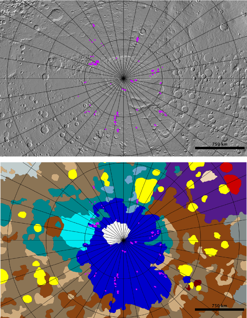
Figure 23: Top: Clean spider distribution overlaid on a MOLA shaded elevation map [84, 70] (top) and over on the geologic map from [72] (bottom). For both plots, latitude and longitude lines are plotted every 10 degrees. A legend for the geologic map is provided in A.

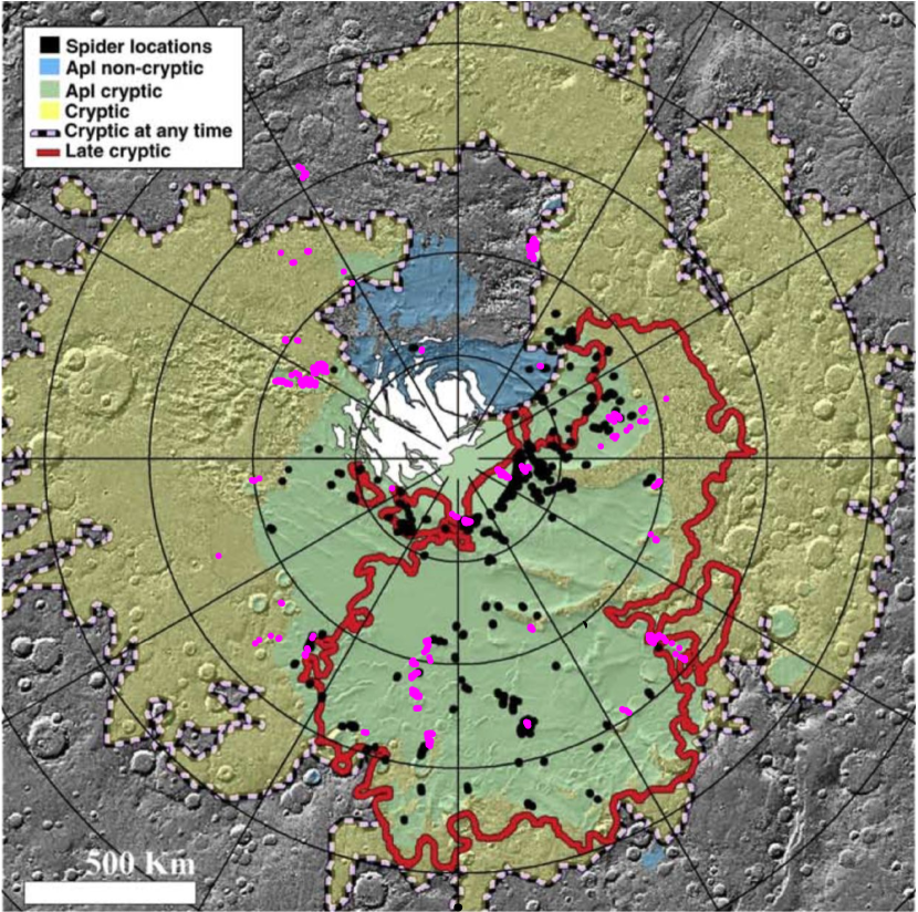
Figure 24: Comparison of P4T clean spider distribution with that of [57]. We overlay our distribution on Figure 2a of [57]. Plotted in magenta is the clean spider sample from this work. The black points are the spider identifications from [57]. The black and white dashed line encloses polar areas that [57] found exhibited cryptic behavior (and thus the presence of semi-translucent slab ice CO₂ ) at any point between Ls = 180^∘ and Ls = 250^∘. The red solid line [57] identifies as cryptic terrain from Ls = 190^∘ onward.An older definition for the SPLD (Amazonian polar polar layered deposit [APL]) [Kolb et al., 2003] is shown in green and blue based on the albedo of the regions between Ls = 180^∘ and Ls = 250^∘) regions. Green represents SPLD areas that exhibited cryptic behavior, and blue are parts of the SPLD that did not exhibit cryptic characteristics as identified by [57]. A visual comparison of the [57] spider identifications find that the locations of nearly all are within the outline of SPLD in the more modern geologic mapping by [72]. Latitude lines are plotted every 5 degrees and longitude lines are plotted every 30 degrees.

Figure 29: Representative sample of each of the regions identified in the clean spider sample as outside of the SPLD unit, continued. Planet Four: Terrains subjects derived from CTX images P13$\_$006151$\_$0974 and P13$\_$006148$\_$1028 .Each P4T subject image is $\sim$4.8$\times 3.6$ km.

Figure 30: Representative sample of each of the regions identified in the clean spider sample as outside of the SPLD unit, continued. Planet Four: Terrains subjects derived from CTX images P13$\_$006148$\_$1028 and G14$\_$023634$\_$103. Each P4T subject image is $\sim$4.8$\times 3.6$ km.

Figure 31: Representative sample of each of the regions identified in the clean spider sample as outside of the SPLD unit, continued. Planet Four: Terrains subjects derived from CTX images P13$\_$006151$\_$0974 and P13$\_$006283$\_$1003. Each P4T subject image is $\sim$4.8$\times 3.6$ km.

6 Comparison to the Swiss Cheese Distribution

In Figure 32, we compare the locations of our clean spider sample to our clean Swiss cheese terrain distribution. There is a clear separation between the locations of the spiders and Swiss cheese terrain in our clean samples. As expected, Swiss cheese terrain is concentrated on the SPRC, the only location on the Martian South polar region that has exposed carbon dioxide ice present at all times of the Martian year. Of the 1,537 subjects identified as containing Swiss cheese terrain, only 10 are located outside of the SPRC region latitudes northward of -80^∘ (subject identifiers: 1070921, 1046056, 1058252, 1058338, 1058430, 1058511, 1058604, 1510352, 485480, and 1510512). In our clean Swiss cheese and spider samples. we find no subjects identified as containing both Swiss cheese terrain and spiders. Our coverage of the South Polar region is moderate with 11$\%$ surface area covered, but this result is consistent with the CO₂ slab ice hypothesis for the production of araneiforms, as the locations identified fall in regions that have been observed to darken in albedo at some point during the thawing of the seasonal CO₂ ice sheet. [9] have recently identified dark fans emanating from exclusively on the sides of mesas in the SPRC. Given the restriction locations of seasonal fan activity mesa walls, this may suggest that araneiforms should not form on the SPRC.

The dissected mesas, linear troughs, moats, and quasi-circular pits characteristic of the SPRC form where there is carbon dioxide ice that persists through the southern summer [e.g. 79]. The 10 subject images outside of the SPRC boundary represent 0.65$\%$ of our clean Swiss cheese sample. Thus, our results are generally consistent with the previously mapped extent of the SPRC [e.g. 75], but indicate some newly discovered regions where carbon dioxide ice likely persists through the southern summer. Of the 10 deviant subjects from the clean Swiss cheese sample lying outside of the SPRC area (Figure 33), 6 are clustered around 78.487^∘ and 101.61^∘ E (CTX image: P13$\_$006290$\_$1017), in the periglacially-deformed thin mantling deposit topping the Hesperian polar unit [72].

Figure 32: Distribution of the clean spider sample and clean Swiss cheese sample on the Martian South Polar region overlaid on a MOLA shaded elevation map [84, 70] (top) and over on the geologic map from [72] (bottom). For both plots, latitude and longitude lines are plotted every 10 degrees. Swiss cheese terrain are identified as the mint green square markers. Spiders are identified as magenta squares. The zero meridian is pointing straight up. A legend for the geologic map is provided in A.

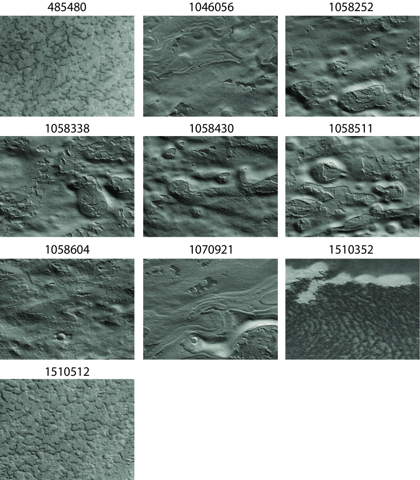
Figure 33: The subjects comprising the Swiss cheese clean sample outside of the SPRC northward of -80^∘ N. Expert review would not classify these images as Swiss cheese, features in these images have some morphologically similarities to Swiss cheese. These 10 images are subimages of CTX frames: G13$\_$023432$\_$1026, P13$\_$006290$\_$1017, P13$\_$005958$\_$1030, G14$\_$023687$\_$1031, and D14$\_$032733$\_$1028. Each P4T subject image is $\sim$4.8$\times 3.6$ km.

7 HiRISE Observations and Interpretations of Candidate Araneiform Locations Outside of the SPLD

To confirm the araneiform identifications outside of the SPLD (presented in Section 5), HiRISE targeted and imaged near these locations in the Southern spring and summer of Mars Year 33. Additionally, we visually inspected all observations outside of the SPLD with $s_{i}{(\textrm{s}pider)}$ greater than 0.5, and the most promising candidates were also added to the HiRISE target database during this time period. With 12-18 times finer spatial resolution than CTX, HiRISE can reveal detail not visible in the original CTX images including whether or not fans are present at the same locations of the candidate spider channels. We present these HiRISE observations obtained to date and discuss each region below. Table 4 lists the HiRISE targets imaged so far, the relevant observations, and the informal names given to each HiRISE target. Figure 34 plots the HiRISE pointings overlaid on a MOLA elevation map [84, 70] and the geologic map from [72]. Overall, seasonal fans were visible in the early spring observations at these locations, confirming CO₂ jet activity consistent with other araneiform locations on the Martian South Polar region [20]. Although these observations are not ice free, dendritic-like channels with similar morphologies to previous HiRISE observations of araneiforms [e.g 20] are visible. Thus, we positively identify araneiforms outside of the SPLD. In this Section, we briefly summarize the characteristics of the araneiform morphologies, if present at each HiRISE target location and present our interpretations based on the high resolution imagery.

Table 4: Candidate Araneiform Locations Outside of the SPLD Targeted by HiRISE

Latitude	Longitude	Informal Name	HiRISE Image IDs
(degrees)	(degrees)
-74.99	330.98	Hempstead	ESP$\_$046948$\_$1050
-77.07	319.00	Bethpage	ESP$\_$046421$\_$1030/ESP$\_$046777$\_$1030$/$ESP$\_$048056$\_$1030
-77.15	227.76	Stony Brook	ESP$\_$046398$\_$1030
-78.54	298.10	Shoram	ESP$\_$046712$\_$1015
-79.46	74.34	Montauk	ESP$\_$046562$\_$1005
-79.49	18.77	Hauppauge	ESP$\_$046564$\_$1005
-80.53	306.10	Dix Hills	ESP$\_$046448$\_$0995$/$ESP$\_$046870$\_$0995/ESP$\_$047938$\_$0995
-82.02	302.31	Patchogue	ESP$\_$046567$\_$0980

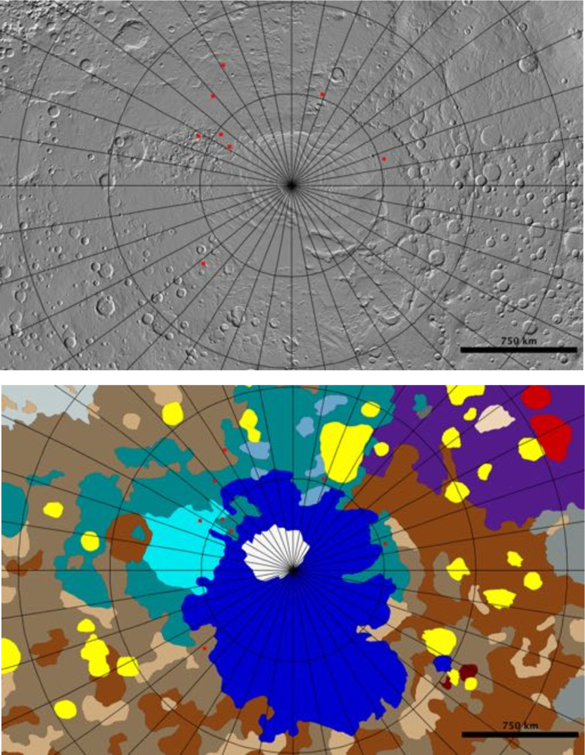
Figure 34: Follow-up HiRISE imaging target locations are shown as the red squares overlaid on top of the MOLA shaded elevation map [84, 70] (top) and geologic map (bottom) from [72]. The plot marker is not to scale of the HiRISE image area. For both plots, latitude and longitude lines are plotted every 10 degrees. The zero meridian is pointing straight up. The zero meridian is pointing straight up. A legend for the geologic map is provided in A.

7.1 Boulders and Fans: Hempstead and Shoram

At -74.81^∘ latitude Hempstead is the furthest site from the Martian South Polar region that is outside of the SPLD. Spiders are primarily centered around boulders, the bright points at the center of the spiders. The region informally nicknamed ‘Inca City’ (latitude = -81.3^∘ N, longitude= 295.7^∘) was previously the only known location with araneiforms and boulders. Fans emanate from the boulders in Hempstead, similar to Inca City. See Figure 35 for a comparison with ESP$\_$029741$\_$0985 from Inca City. Like Inca City, the boulders appear to spur the generation of the carbon dioxide jets. As proposed by [73], the boulders are surrounded and covered by the seasonal ice sheet. The boulders provide a discontinuity in thermal inertia and an additional source of thermal heat that enables the surrounding ice to sublimate and crack more easily providing an outlet for the trapped carbon dioxide gas. As we see at Shoram (Figure 36) it is not always a simple story, however. In Shoram there are also small boulders, but they are not always associated with fans.

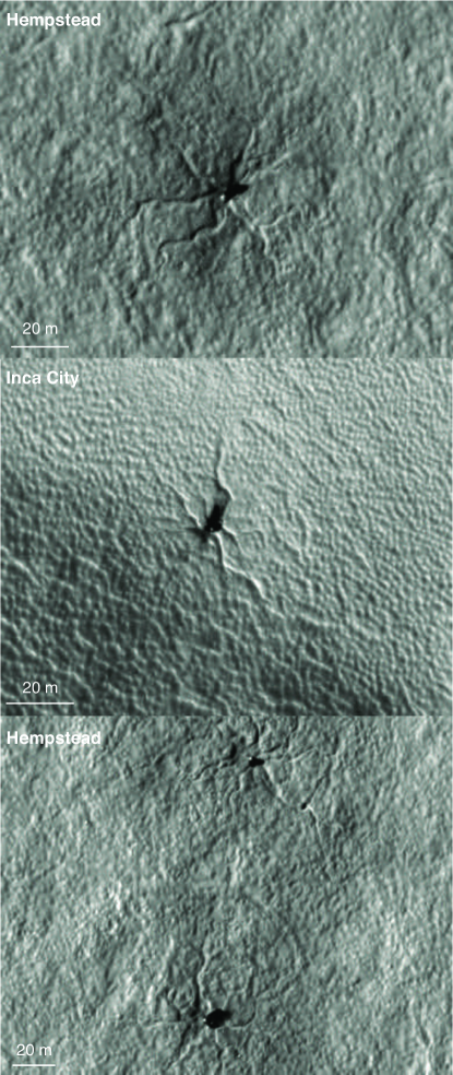
Figure 35: Hempstead spiders (ESP$\_$046948$\_$1050;L_s=196.2^∘) compared to an Inca City spider (ESP$\_$029741$\_$0985;L_s=216.2^∘). At the center of each pit is a boulder in all three cutouts. Sinuous channels characteristic of araneiform morphology converge at each boulder/pit location in the cutouts. All three cutouts also show a dark seasonal fan emerging from the center originating at the boulder location indicative of active CO₂ outgassing at these locations.

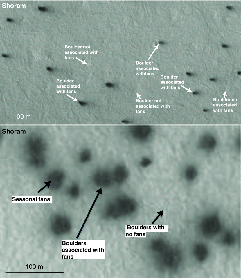
Figure 36: Boulders associated with seasonal activity in Shoram are shown in the top panel, a cutout from HiRISE image ESP$\_$046712$\_$1015, acquired at L_s=185.5^∘. The fine particles deposited on the seasonal ice layer may land in a fan-shaped deposit if the ambient winds are blowing in a particular direction, or just in a directionless blotch if not. Both panels show that seasonal activity at this t L_s is associated with the locations of some boulders but not all.

7.2 Boundaries and Interfaces: Bethpage

Bethpage has narrow channels radiating from broad troughs. A representative close-up is shown in Figure 37. Dark dust on the top of the seasonal ice surrounds the channels as highlighted in Figure 38. The appearance of the seasonal fans is consistent with active CO₂ jet processes on-going in this region, thus we infer that at least the narrow channels are formed by erosion from seasonal CO₂ gas escape entraining loose material from the surface under the seasonal ice. As shown in Figure 39 the broad troughs and narrow channels are found in hummocky terrain and along the boundary of smoother terrain, consistent with the hypothesis that CO₂ jet processes exploit the weaknesses in the regolith to form sinuous araneiform channels.

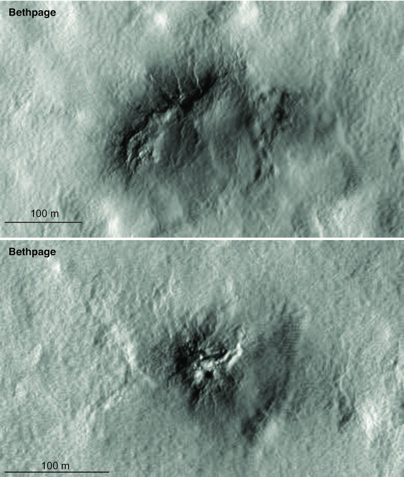
Figure 37: Broad troughs with araneiform-like channels in Bethpage observed by HiRISE (ESP$\_$046777$\_$1030; L_s=188.4^∘).The fans are less distinct in the middle and lower panels, examples of broad troughs and araneiform channels at this time in the Southern spring season, but the seasonal fans deposits are still visible as a darker area in the vicinity of the channels.

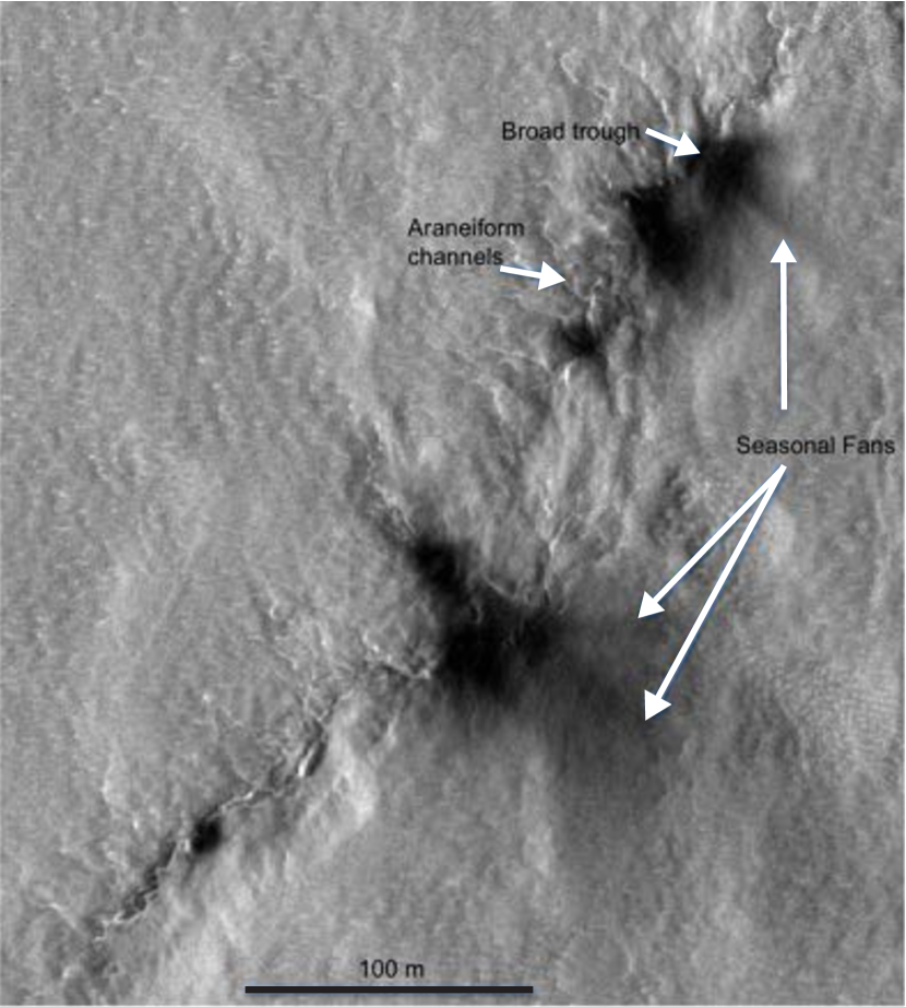
Figure 38: Araneiforms in Bethpage. Dark seasonal fans associated with channels in this Bethpage cutout taken from HiRISE image ESP$\_$046421$\_$1030, acquired at L_s= 172.7^∘).

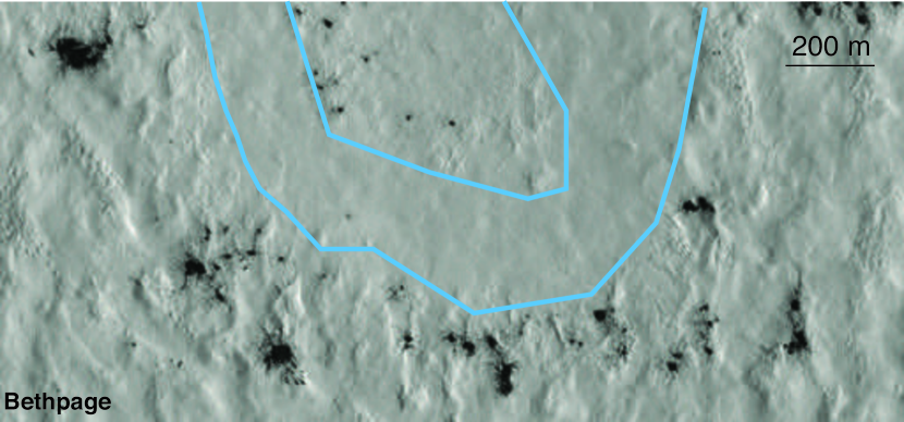
Figure 39: Broad troughs with araneiform like channels in Bethpage observed by HiRISE (ESP$\_$048056$\_$1030; L_s=249.5^∘). At the time the image was taken the surface in this region was covered by a semi-translucent seasonal layer of CO₂ ice. The black patches in the image are seasonal fan material. Seasonal jet activity was found occurring near the boundaries of relatively smooth terrain and more hummocky terrain. Light blue solid lines are drawn at the approximate outline of a smooth region surrounded by hummocky terrain in this HiRISE cutout.

7.3 Short Channels and Boulders: Stony Brook

At Stony Brook the terrain is rough on the scale of meters. There are short channels but with a few exceptions they do not show the branching, dendritic characteristics or the tight sinuosity of the araneiform terrains previously reported in the literature [e.g. 20]. HiRISE image ESP$\_$046398$\_$1030, shown in Figure 40, displays seasonal fans (some coming from boulders and some from short grooves) and a few well-developed spiders. Frosted spider outlines are also visible in the region as well.

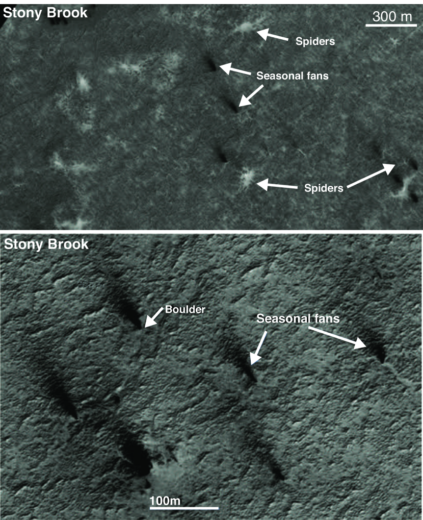
Figure 40: Stony Brook: Frosted spiders and dark seasonal fans are visible in the top two panel, a cutout rom HiRISE image ESP$\_$046398$\_$1030 taken at L_s=171.7^∘. The lower panel shows seasonal fans, visible in ESP$\_$047308$\_$1030, acquired at L_s=213^∘.

7.4 Connected Aaraneiforms: Montauk, Happauge, and Shoram

Montauk has well-developed araneiforms as shown in Figure 41. Separated spiders are visible, but the vast majority of the araneiforms visible in these HiRISE observations are connected spiders, where dendritic channels are not emanating from a point but rather the channels form complex and interlinked networks of araneiform channels. This has a morphology similar to what [20] describes as Connected Araneiform Morphology. Along with having boulders, Shoram also has pockets of connected araneiform features. At L_s=185.5^∘, fans can be seen originating from many of the dendritic channels as shown in Figure 42. Additionally, Happauge (see Figure 43) also exhibits connected araneiforms. The ground surrounding the spiders in Hauppage also has a stippled texture although this may not be related to the seasonal carbon dioxide jets.

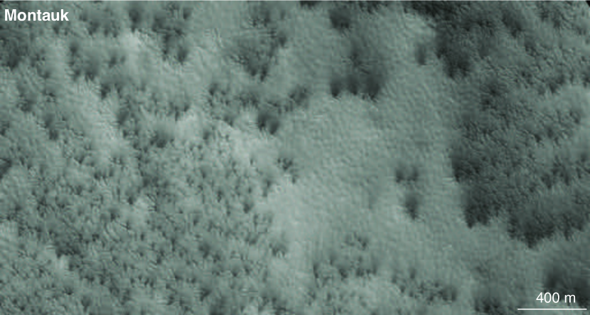
Figure 41: Connected araneiforms in Montauk (ESP$\_$046562$\_$1005; L_s=178.8^∘). In this subimage, branching channels are visible with no central organization. Dark seasonal fans are also present indicating active carbon dioxide CO₂ jets have formed this region.

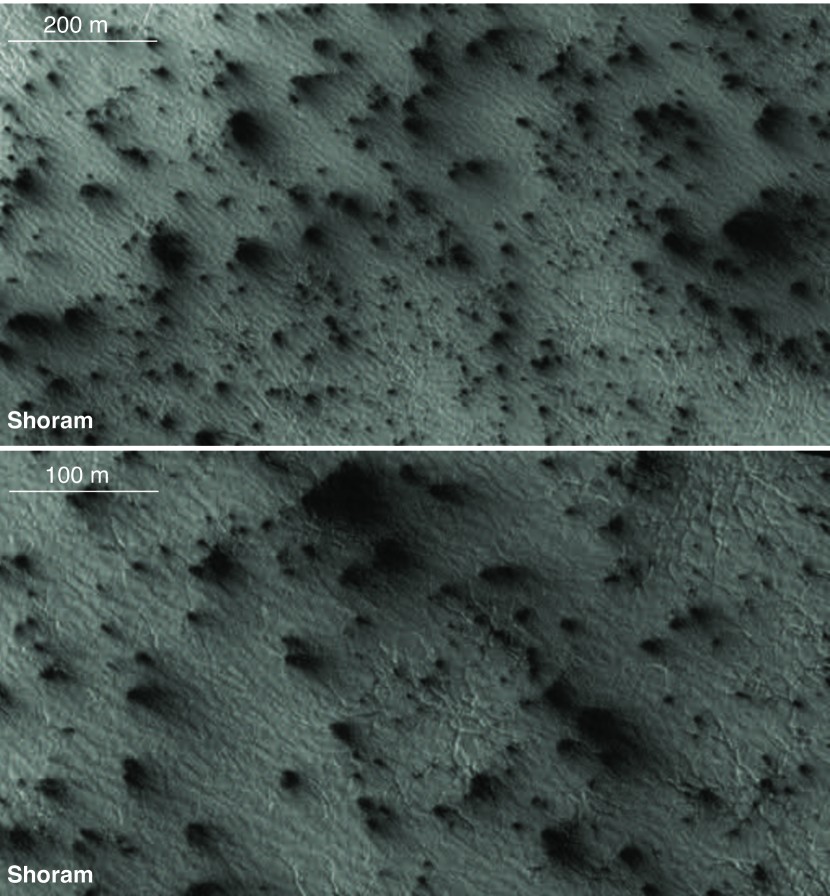
Figure 42: Sample of connected araneiform features identified in HiRISE observations of Shoram (ESP$\_$046712$\_$1015;L_s=185.5^∘). The sinuous channels appear to not be centralized around a single point or surface pit. Dark seasonal fans present at the top of the semi-translucent seasonal CO₂ ice sheet are also visible at this locale. Many of the fans originate at locations above the dendritic araneiform channels.

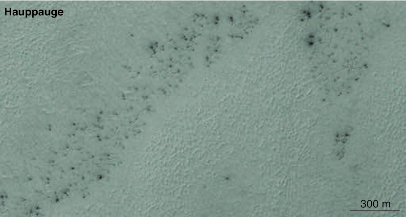
Figure 43: Araneiform morphology in Hauppauge imaged by HiRISE (ESP$\_$046564$\_$1005; L_s=178.9^∘). Dark seasonal fans can be seen on top of the semi-translucent CO₂ ice at locations where dendritic channels are present in the surface below. The terrain in between the araneiforms is stippled in texture.

7.5 Spiders on Possible Eject Blankets: Montauk and Happauge

Montauk is located on the rim of a partially eroded un-named crater (see Figure 44) and Hauppauge is located near a large crater named ‘South Crater’ as shown in Figure 45. These two regions may reside on the crater ejecta blankets. The layering or unconsolidated nature of the surface inherent in an ejecta blanket may provide a conducive environment for spider development, similar to the SPLD, where araneiforms were originally found to reside [see 57]. Identification of crater ejecta is challenging. Only fresh or moderately eroded craters will have ejecta blankets surrounding the crater rim identifiable in orbital images. Following [67], we examined Thermal Emission Imaging System (THEMIS )Day Infrared IR) 100m per pixel global map mosaic [16, 23] of the area surrounding Montauk and Happauge (see Figures 44 and 45). Hauppage appears in the THEMIS observations to be on a darker unit, but it is not clear if this can be identified as part of South Crater’s ejecta blanket. From our analysis we cannot confirm that these locations outside of the SPLD coincide with ejecta blankets. Further high resolution observations and detections of more araneiforms outside of the SPLD in close proximity to crater rims would bolster this hypothesis.

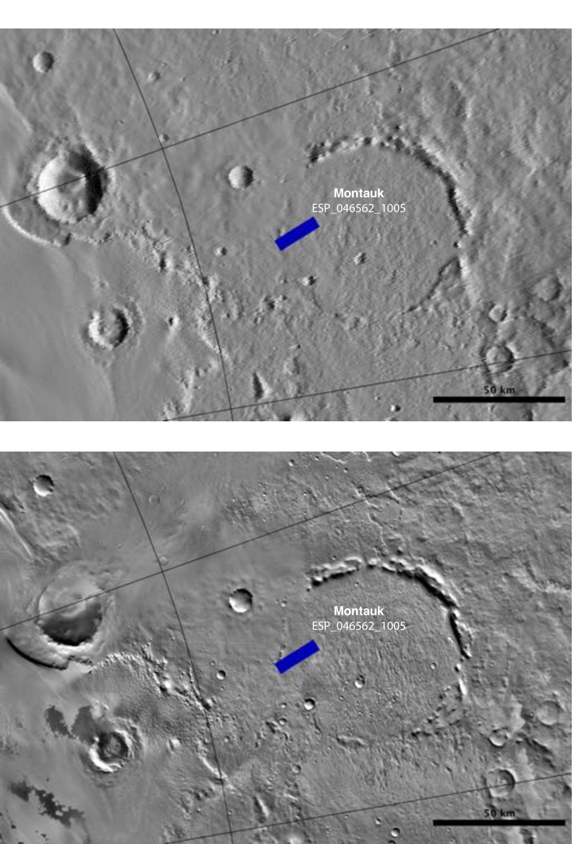
Figure 44: Proximity of Montauk in relation to a nearby crater rim and possible ejecta blanket. The top shows the extent of HiRISE observation ESP$\_$046562$\_$1005 (L_s=178.8^∘) overlaid on a MOLA shaded elevation map [84, 70]. The bottom image displays the HiRISE target overlaid on top of the THEMIS DAY IR 100m global map mosaic [16, 23]. For both figures, latitude and longitude lines are plotted every 10 degrees. The zero meridian is pointing straight up.

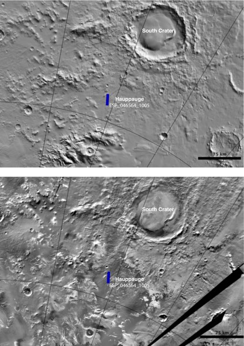
Figure 45: Proximity of Hauppauge to South Crater. The top shows the extent of HiRISE observation ESP$\_$046562$\_$1005 (L_s=178.8^∘) overlaid on a MOLA shaded elevation map [84, 70]. The bottom image displays the HiRISE target overlaid on top of the THEMIS DAY IR 100m global map mosaic [16, 23]. For both figures, latitude and longitude lines are plotted every 10 degrees. The zero meridian is pointing straight up. Hauppage appears in the THEMIS observations to be on a darker unit, but it is not clear if this can be identified as part of South Crater’s ejecta blanket.

7.6 Polygons and Spiders: Dix Hills

Extensive polygonal cracks are visible in the surface at Dix Hills. Polygonal cracks are one of many well-documented types of patterned ground formed by the cyclic freezing and thawing of underlying water ice-cemented ground, and the subsequent cracking of ice-rich material produces shallow grooves[47]. The association of fans with these grooves leads us to infer that they provide routes for the flow of the trapped pressurized gas under the CO₂ seasonal cap. As shown in Figure 46 and Figure 47 more sinuous araneiform channels are also present at these locales. Fans are visible in later observations of Dix Hills where the polygonal channels have pits, are wider, and/or develop secondary branching channels, as shown in Figure 47.

Figure 46: Polygonal channels in the ground are visible at Dix Hills in HiRISE observation ESP$\_$047938$\_$0995 acquired at L_s=243.7^∘. Seasonal fans (dark patches) associated with the channels are evidence for seasonal sub-ice gas flow along the polygonal grooves.

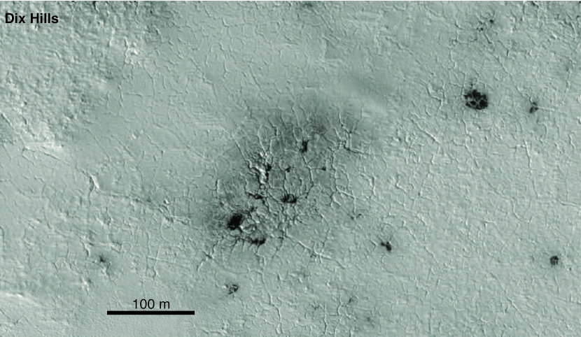
Figure 47: Araneiform terrain located along the polygonal grooves is shown in this cutout of HiRISE image ESP$\_$047938$\_$0995 (L_s=243.7^∘) of Dix Hills. Seasonal fan (dark black patches in the image) are associated with some of the araneiform channels, indicating active CO₂ jets at these locations.

7.7 Sinuous Channels: Patchogue

Patchogue has both sinuous channels and distinct well-separated spiders, with distinctly visible central pits and radiating channels, see Figure 48. The spiders’ morphology is the classic spider with radially-organized channels, that have been observed by HiRISE on other locales on the SPLD [20]. Patchogue is near Inca City, but unlike Hempstead, Shoram, and Inca City, no boulders were visible.

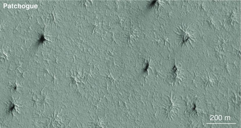
Figure 48: Sample of spider araneiform features identified in HiRISE observations of Patchogue (ESP$\_$046567$\_$0980; L_s=179.1^∘). Distinct spiders are visible with sinuous channels emanating from a central pit. At this L_s, some of the isolated spiders also exhibit seasonal fans at the locations above on the top of the seasonal ice sheet.

8 Implications for the CO₂ Jet Model

The majority of the P4T clean spider sample ( $75\%$) resides on the SPLD, where the carbon dioxide jet model has been previously put forth for the formation of araneiforms [30, 57, 32, 31, 58, 73, 63, 55, 74]. High resolution HiRISE imaging confirms the identification of several locations outside of the SPLD with araneiforms found by P4T. All of the HiRISE observations of the locales outside of the SPLD with confirmed araneiform features visible, also exhibited seasonal fans, suggesting that active CO₂ jets were present during the season. Additionally, all but one of these HiRISE target locations have already been identified by [57] as becoming cryptic (with temperatures near the CO₂ frost sublimation temperature but with an albedo lower than that of typical CO₂ frost) for a period of time between L_S = 180^∘ and L_S = 250^∘, indicative of semi-translucent CO₂ slab ice required for the CO₂ jet formation. For Hempstead, there was no albedo information available to [57], but [59] identify the presence of the seasonal ice cap extending beyond that location to -50^∘ over multiple Mars years. Thus our clean spider distribution and new araneiform discoveries outside of the SPLD are consistent with the preferred CO₂ jet model and slab ice formation model.

Our outside of the SPLD spider identifications are located in Amazonian and Hesperian polar units and the Early Noachian highland units outside of the SPLD. With our current coverage of $\sim$11$\%$ of the South Polar region southward of 75^∘, we cannot make a definitive statement regarding whether these are the only geologic units with araneiforms within the Martian South Polar region. A larger search for araneiforms in CTX and MOC NA observations are needed. The presence araneiforms in the new areas identified in this study suggests that the regolith in these areas can be easily weakened or is loosely conglomerated like that of the SPLD, enabling the trapped carbon dioxide gas to slowly carve channels into the surface over time. Further study of the surface properties may illuminate the link between the SPLD and these regions for araneiform formation. Two of the HiRISE target locations (Hauppague and Montauk) are close to craters and may reside on associated ejecta blankets. This may indicate that crater ejecta blankets play an important role in the formation of araneiforms outside of the SPLD as an alternative source for loosely conglomerated materials to excavate. Further HiRISE observations and samples of araneiforms outside the SPLD are needed before a definitive conclusion can be made.

9 Conclusions

Through the effort of over 10,000 volunteers, P4T has mapped the distribution of spider araneiforms in 90 CTX observations of the Martian South Pole. This paper presents results from our analysis of 303,192 km² of CTX observations between -75^∘ and the South Pole, mapping locations of araneiforms and Swiss cheese terrain on the Martian South Pole. We present the first identification of araneiforms present at locations outside the SPLD. This discovery is consistent with the general paradigm where the CO₂ jet process carves channels into the surface by the trapped CO₂ gas exploiting weaknesses in the conglomeration of the soil layer below [30, 57, 32, 31, 58, 73, 63, 55, 74].

Although the spiders are found primarily on the SPLD, the source of the non-uniformity of the spider distribution requires further study. The morphology of the aranieforms and rate of the erosion process to carve channels into the surfaces outside the SPLD is likely a combination of material strength of the surface, surface slopes, and the amount of time the seasonal CO₂ ice sheet is present at each location. We find that several of our newly identified araneiform locales are on or close to crater ejecta blankets. With our limited sample size, we can not definitively conclude that araneiform formation outside of the SPLD prefers disturbed regolith such as crater ejecta blankets. A larger survey of the South Polar region is required. Further high resolution imaging of these new spider locations coupled with additional surveys of the South Polar region will further elucidate the formation of these features and the CO₂ seasonal jet process.

10 Future Prospects

The success of P4T in providing timely targets for follow-up high resolution imaging highlights citizen science and crowd sourcing as a potential future avenue for efficiently identifying planetary surface features in planetary mission datasets and feeding back into mission planning. The area searched by P4T presented in this Paper was constrained in order to have both the citizen science review and full analysis of the classifications completed before the beginning of the South spring Equinox in Mars Year 33 and the start of HiRISE’s seasonal processes monitoring campaign. With the completion of this first set of 90 CTX observations, additional CTX images have continued to be available on the P4T website for review; expanding the coverage wider beyond -75^∘ latitude. Classification of these images is currently underway. We expect in future works to be able to produce a sample of baby spider and channel network locations from P4T classifications. P4T will be able to further examine the abundance of spiders outside the SPLD and the correlations with surface properties that can shed light on how the CO₂ jet process is able to carve channels into the SPLD and these other regions of the South Pole. More examples of araneiform locations outside of the SPLD will enable a better analysis of the prevalence of crater ejecta blankets as suitable environments from araneiform formation.

Appendix A Geologic Map Legend

We provide in Figure 49 a legend identifying the main geologic units of the South Polar region in the geologic map from [72] used in this work. We refer the reader to [72] for further details about the characteristics of each geologic unit. We note that the Amazonian polar undivided unit is also known as the South Polar Layered Deposits (SPLD), and the Late Amazonian polar cap unit is also referred to as the South Polar Residual Cap (SPRC).

Figure 49: Main geologic units comprising the South Polar region of Mars as identified by [72]. Latitude and longitude lines are plotted every 10 degrees. The zero meridian is pointing straight up.

References

References

- Aharonson et al. [2004] Aharonson, O., Zuber, M.T., Smith, D.E., Neumann, G.A., Feldman, W.C., Prettyman, T.H., 2004. Depth, distribution, and density of CO2 deposition on Mars. Journal of Geophysical Research (Planets) 109, E05004. doi:10.1029/2003JE002223.
- Anderson et al. [2004] Anderson, J.A., Sides, S.C., Soltesz, D.L., Sucharski, T.L., Becker, K.J., 2004. Modernization of the Integrated Software for Imagers and Spectrometers, in: Mackwell, S., Stansbery, E. (Eds.), Lunar and Planetary Science Conference, p. 2039.
- Astropy Collaboration et al. [2013] Astropy Collaboration, Robitaille, T.P., Tollerud, E.J., Greenfield, P., Droettboom, M., Bray, E., Aldcroft, T., Davis, M., Ginsburg, A., Price-Whelan, A.M., Kerzendorf, W.E., Conley, A., Crighton, N., Barbary, K., Muna, D., Ferguson, H., Grollier, F., Parikh, M.M., Nair, P.H., Unther, H.M., Deil, C., Woillez, J., Conseil, S., Kramer, R., Turner, J.E.H., Singer, L., Fox, R., Weaver, B.A., Zabalza, V., Edwards, Z.I., Azalee Bostroem, K., Burke, D.J., Casey, A.R., Crawford, S.M., Dencheva, N., Ely, J., Jenness, T., Labrie, K., Lim, P.L., Pierfederici, F., Pontzen, A., Ptak, A., Refsdal, B., Servillat, M., Streicher, O., 2013. Astropy: A community Python package for astronomy. A&A 558, A33. doi:10.1051/0004-6361/201322068, arXiv:1307.6212.
- Becerra et al. [2015] Becerra, P., Byrne, S., Brown, A.J., 2015. Transient bright ’’halos’’ on the South Polar Residual Cap of Mars: Implications for mass-balance. Icarus 251, 211--225. doi:10.1016/j.icarus.2014.04.050.
- Becker et al. [2007] Becker, K.J., Anderson, J.A., Sides, S.C., Miller, E.A., Eliason, E.M., Keszthelyi, L.P., 2007. Processing HiRISE Images Using ISIS3, in: Lunar and Planetary Science Conference, p. 1779.
- Benson and James [2005] Benson, J.L., James, P.B., 2005. Yearly comparisons of the martian polar caps: 1999 2003 Mars Orbiter Camera observations. Icarus 174, 513--523. doi:10.1016/j.icarus.2004.08.025.
- Bierson et al. [2016] Bierson, C.J., Phillips, R.J., Smith, I.B., Wood, S.E., Putzig, N.E., Nunes, D., Byrne, S., 2016. Stratigraphy and evolution of the buried CO2 deposit in the Martian south polar cap. Geophys. Res. Lett. 43, 4172--4179. doi:10.1002/2016GL068457.
- Bugiolacchi et al. [2016] Bugiolacchi, R., Bamford, S., Tar, P., Thacker, N., Crawford, I.A., Joy, K.H., Grindrod, P.M., Lintott, C., 2016. The Moon Zoo citizen science project: Preliminary results for the Apollo 17 landing site. Icarus 271, 30--48. doi:10.1016/j.icarus.2016.01.021, arXiv:1602.01664.
- Buhler et al. [2017] Buhler, P.B., Ingersoll, A.P., Ehlmann, B.L., Fassett, C.I., Head, J.W., 2017. How the martian residual south polar cap develops quasi-circular and heart-shaped pits, troughs, and moats. Icarus 286, 69--93. doi:10.1016/j.icarus.2017.01.012.
- Byrne and Ingersoll [2003] Byrne, S., Ingersoll, A.P., 2003. A Sublimation Model for Martian South Polar Ice Features. Science 299, 1051--1053. doi:10.1126/science.1080148.
- Christensen et al. [2009] Christensen, P.R., Engle, E., Anwar, S., Dickenshied, S., Noss, D., Gorelick, N., Weiss-Malik, M., 2009. JMARS - A Planetary GIS. AGU Fall Meeting Abstracts .
- Clancy et al. [2000] Clancy, R.T., Sandor, B.J., Wolff, M.J., Christensen, P.R., Smith, M.D., Pearl, J.C., Conrath, B.J., Wilson, R.J., 2000. An intercomparison of ground-based millimeter, MGS TES, and Viking atmospheric temperature measurements: Seasonal and interannual variability of temperatures and dust loading in the global Mars atmosphere. J. Geophys. Res. 105, 9553--9572. doi:10.1029/1999JE001089.
- Clifford et al. [2000] Clifford, S.M., Crisp, D., Fisher, D.A., Herkenhoff, K.E., Smrekar, S.E., Thomas, P.C., Wynn-Williams, D.D., Zurek, R.W., Barnes, J.R., Bills, B.G., Blake, E.W., Calvin, W.M., Cameron, J.M., Carr, M.H., Christensen, P.R., Clark, B.C., Clow, G.D., Cutts, J.A., Dahl-Jensen, D., Durham, W.B., Fanale, F.P., Farmer, J.D., Forget, F., Gotto-Azuma, K., Grard, R., Haberle, R.M., Harrison, W., Harvey, R., Howard, A.D., Ingersoll, A.P., James, P.B., Kargel, J.S., Kieffer, H.H., Larsen, J., Lepper, K., Malin, M.C., McCleese, D.J., Murray, B., Nye, J.F., Paige, D.A., Platt, S.R., Plaut, J.J., Reeh, N., Rice, J.W., Smith, D.E., Stoker, C.R., Tanaka, K.L., Mosley-Thompson, E., Thorsteinsson, T., Wood, S.E., Zent, A., Zuber, M.T., Jay Zwally, H., 2000. The State and Future of Mars Polar Science and Exploration. Icarus 144, 210--242. doi:10.1006/icar.1999.6290.
- Cutts [1973] Cutts, J.A., 1973. Nature and origin of layered deposits of the Martian polar region. J. Geophys. Res. 78, 4231--4249. doi:10.1029/JB078i020p04231.
- de Villiers et al. [2012] de Villiers, S., Nermoen, A., Jamtveit, B., Mathiesen, J., Meakin, P., Werner, S.C., 2012. Formation of Martian araneiforms by gas-driven erosion of granular material. Geophys. Res. Lett. 39, L13204. doi:10.1029/2012GL052226.
- Edwards et al. [2011] Edwards, C.S., Nowicki, K.J., Christensen, P.R., Hill, J., Gorelick, N., Murray, K., 2011. Mosaicking of global planetary image datasets: 1. Techniques and data processing for Thermal Emission Imaging System (THEMIS) multi-spectral data. Journal of Geophysical Research (Planets) 116, E10008. doi:10.1029/2010JE003755.
- Fischer et al. [2012] Fischer, D.A., Schwamb, M.E., Schawinski, K., Lintott, C., Brewer, J., Giguere, M., Lynn, S., Parrish, M., Sartori, T., Simpson, R., Smith, A., Spronck, J., Batalha, N., Rowe, J., Jenkins, J., Bryson, S., Prsa, A., Tenenbaum, P., Crepp, J., Morton, T., Howard, A., Beleu, M., Kaplan, Z., Vannispen, N., Sharzer, C., Defouw, J., Hajduk, A., Neal, J.P., Nemec, A., Schuepbach, N., Zimmermann, V., 2012. Planet Hunters: the first two planet candidates identified by the public using the Kepler public archive data. MNRAS 419, 2900--2911. doi:10.1111/j.1365-2966.2011.19932.x, arXiv:1109.4621.
- Fortson et al. [2012] Fortson, L., Masters, K., Nichol, R., Borne, K.D., Edmondson, E.M., Lintott, C., Raddick, J., Schawinski, K., Wallin, J., 2012. Galaxy Zoo: Morphological Classification and Citizen Science. pp. 213--236.
- Genova et al. [2016] Genova, A., Goossens, S., Lemoine, F.G., Mazarico, E., Neumann, G.A., Smith, D.E., Zuber, M.T., 2016. Seasonal and static gravity field of Mars from MGS, Mars Odyssey and MRO radio science. Icarus 272, 228--245. doi:10.1016/j.icarus.2016.02.050.
- Hansen et al. [2010] Hansen, C.J., Thomas, N., Portyankina, G., McEwen, A., Becker, T., Byrne, S., Herkenhoff, K., Kieffer, H., Mellon, M., 2010. HiRISE observations of gas sublimation-driven activity in Mars’southern polar regions: I. Erosion of the surface. Icarus 205, 283--295. doi:10.1016/j.icarus.2009.07.021.
- Herkenhoff and Plaut [2000] Herkenhoff, K.E., Plaut, J.J., 2000. Surface Ages and Resurfacing Rates of the Polar Layered Deposits on Mars. Icarus 144, 243--253. doi:10.1006/icar.1999.6287.
- Hess et al. [1979] Hess, S.L., Henry, R.M., Tillman, J.E., 1979. The seasonal variation of atmospheric pressure on Mars as affected by the south polar CAP. J. Geophys. Res. 84, 2923--2927. doi:10.1029/JB084iB06p02923.
- Hill et al. [2014] Hill, J., Edwards, C.S., Christensen, P.R., 2014. Mapping the Martian Surface with THEMIS Global Infrared Mosaics, in: Eighth International Conference on Mars, p. 1141.
- James et al. [2001] James, P.B., Cantor, B.A., Davis, S., 2001. Mars Orbiter Camera observations of the Martian south polar cap in 1999-2000. J. Geophys. Res. 106, 23635--23652. doi:10.1029/2000JE001313.
- James et al. [1992] James, P.B., Kieffer, H.H., Paige, D.A., 1992. The seasonal cycle of carbon dioxide on Mars. pp. 934--968.
- James et al. [2010] James, P.B., Thomas, P.C., Malin, M.C., 2010. Variability of the south polar cap of Mars in Mars years 28 and 29. Icarus 208, 82--85. doi:10.1016/j.icarus.2010.02.007.
- Kaufmann and Hagermann [2017] Kaufmann, E., Hagermann, A., 2017. Experimental investigation of insolation-driven dust ejection from mars’ {CO2} ice caps. Icarus 282, 118 -- 126. doi:http://dx.doi.org/10.1016/j.icarus.2016.09.039.
- Kelly et al. [2006] Kelly, N.J., Boynton, W.V., Kerry, K., Hamara, D., Janes, D., Reedy, R.C., Kim, K.J., Haberle, R.M., 2006. Seasonal polar carbon dioxide frost on Mars: CO2 mass and columnar thickness distribution. Journal of Geophysical Research (Planets) 111, E03S07. doi:10.1029/2006JE002678.
- Kieffer [1979] Kieffer, H.H., 1979. Mars south polar spring and summer temperatures - A residual CO2 frost. J. Geophys. Res. 84, 8263--8288. doi:10.1029/JB084iB14p08263.
- Kieffer [2000] Kieffer, H.H., 2000. Annual Punctuated CO2 Slab-Ice and Jets on Mars, in: Second International Conference on Mars Polar Science and Exploration, p. 93.
- Kieffer [2007] Kieffer, H.H., 2007. Cold jets in the Martian polar caps. Journal of Geophysical Research (Planets) 112, E08005. doi:10.1029/2006JE002816.
- Kieffer et al. [2006] Kieffer, H.H., Christensen, P.R., Titus, T.N., 2006. CO2 jets formed by sublimation beneath translucent slab ice in Mars’ seasonal south polar ice cap. Nature 442, 793--796. doi:10.1038/nature04945.
- Kieffer et al. [2000] Kieffer, H.H., Titus, T.N., Mullins, K.F., Christensen, P.R., 2000. Mars south polar spring and summer behavior observed by TES: Seasonal cap evolution controlled by frost grain size. J. Geophys. Res. 105, 9653--9700. doi:10.1029/1999JE001136.
- Kieffer and Zent [1992] Kieffer, H.H., Zent, A.P., 1992. Quasi-periodic climate change on Mars. pp. 1180--1218.
- Kraft et al. [1991] Kraft, R.P., Burrows, D.N., Nousek, J.A., 1991. Determination of confidence limits for experiments with low numbers of counts. ApJ 374, 344--355. doi:10.1086/170124.
- Kuchner et al. [2016] Kuchner, M.J., Silverberg, S.M., Bans, A.S., Bhattacharjee, S., Kenyon, S.J., Debes, J.H., Currie, T., Garcia, L., Jung, D., Lintott, C., McElwain, M., Padgett, D.L., Rebull, L.M., Wisniewski, J.P., Nesvold, E., Schawinski, K., Thaller, M.L., Grady, C.A., Biggs, J., Bosch, M., Cernohous, T., Durantini Luca, H.A., Hyogo, M., Wah, L.L.W., Piipuu, A., Piñeiro, F., 2016. Disk Detective: Discovery of New Circumstellar Disk Candidates through Citizen Science. ArXiv e-prints arXiv:1607.05713.
- Landis et al. [2016] Landis, M.E., Byrne, S., Daubar, I.J., Herkenhoff, K.E., Dundas, C.M., 2016. A revised surface age for the North Polar Layered Deposits of Mars. Geophys. Res. Lett. 43, 3060--3068. doi:10.1002/2016GL068434.
- Leighton and Murray [1966] Leighton, R.B., Murray, B.C., 1966. Behavior of Carbon Dioxide and Other Volatiles on Mars. Science 153, 136--144. doi:10.1126/science.153.3732.136.
- Lintott et al. [2011] Lintott, C., Schawinski, K., Bamford, S., Slosar, A., Land, K., Thomas, D., Edmondson, E., Masters, K., Nichol, R.C., Raddick, M.J., Szalay, A., Andreescu, D., Murray, P., Vandenberg, J., 2011. Galaxy Zoo 1: data release of morphological classifications for nearly 900 000 galaxies. MNRAS 410, 166--178. doi:10.1111/j.1365-2966.2010.17432.x, arXiv:1007.3265.
- Lintott et al. [2008] Lintott, C.J., Schawinski, K., Slosar, A., Land, K., Bamford, S., Thomas, D., Raddick, M.J., Nichol, R.C., Szalay, A., Andreescu, D., Murray, P., Vandenberg, J., 2008. Galaxy Zoo: morphologies derived from visual inspection of galaxies from the Sloan Digital Sky Survey. MNRAS 389, 1179--1189. doi:10.1111/j.1365-2966.2008.13689.x, arXiv:0804.4483.
- Litvak et al. [2007] Litvak, M.L., Mitrofanov, I.G., Kozyrev, A.S., Sanin, A.B., Tretyakov, V.I., Boynton, W.V., Kelly, N.J., Hamara, D., Saunders, R.S., 2007. Long-term observations of southern winters on Mars: Estimations of column thickness, mass, and volume density of the seasonal CO2 deposit from HEND/Odyssey data. Journal of Geophysical Research (Planets) 112, E03S13. doi:10.1029/2006JE002832.
- Malin et al. [2007] Malin, M.C., Bell, J.F., Cantor, B.A., Caplinger, M.A., Calvin, W.M., Clancy, R.T., Edgett, K.S., Edwards, L., Haberle, R.M., James, P.B., Lee, S.W., Ravine, M.A., Thomas, P.C., Wolff, M.J., 2007. Context Camera Investigation on board the Mars Reconnaissance Orbiter. Journal of Geophysical Research (Planets) 112, E05S04. doi:10.1029/2006JE002808.
- Malin et al. [2001] Malin, M.C., Caplinger, M.A., Davis, S.D., 2001. Observational Evidence for an Active Surface Reservoir of Solid Carbon Dioxide on Mars. Science 294, 2146--2148. doi:10.1126/science.1066416.
- Malin et al. [1992] Malin, M.C., Danielson, G.E., Ingersoll, A.P., Masursky, H., Veverka, J., Ravine, M.A., Soulanille, T.A., 1992. Mars Observer camera. J. Geophys. Res. 97, 7699--7718. doi:10.1029/92JE00340.
- Malin and Edgett [2001] Malin, M.C., Edgett, K.S., 2001. Mars Global Surveyor Mars Orbiter Camera: Interplanetary cruise through primary mission. J. Geophys. Res. 106, 23429--23570. doi:10.1029/2000JE001455.
- Malin et al. [2010] Malin, M.C., Edgett, K.S., Cantor, B.A., Caplinger, M.A., Danielson, G.E., Jensen, E.H., Ravine, M.A., Sandoval, J.L., Supulver, K.D., 2010. An overview of the 1985-2006 Mars Orbiter Camera science investigation. International Journal of Mars Science and Exploration 5, 1--60. doi:10.1555/mars.2010.0001.
- Mangold [2005] Mangold, N., 2005. High latitude patterned grounds on Mars: Classification, distribution and climatic control. Icarus 174, 336--359. doi:10.1016/j.icarus.2004.07.030.
- Marshall et al. [2015] Marshall, P.J., Lintott, C.J., Fletcher, L.N., 2015. Ideas for Citizen Science in Astronomy. ARA&A 53, 247--278. doi:10.1146/annurev-astro-081913-035959, arXiv:1409.4291.
- Matsuo and Heki [2009] Matsuo, K., Heki, K., 2009. Seasonal and inter-annual changes of volume density of martian CO 2 snow from time-variable elevation and gravity. Icarus 202, 90--94. doi:10.1016/j.icarus.2009.02.023.
- McEwen et al. [2007] McEwen, A.S., Eliason, E.M., Bergstrom, J.W., Bridges, N.T., Hansen, C.J., Delamere, W.A., Grant, J.A., Gulick, V.C., Herkenhoff, K.E., Keszthelyi, L., Kirk, R.L., Mellon, M.T., Squyres, S.W., Thomas, N., Weitz, C.M., 2007. Mars Reconnaissance Orbiter’s High Resolution Imaging Science Experiment (HiRISE). Journal of Geophysical Research (Planets) 112, E05S02. doi:10.1029/2005JE002605.
- McEwen et al. [2011] McEwen, A.S., Ojha, L., Dundas, C.M., Mattson, S.S., Byrne, S., Wray, J.J., Cull, S.C., Murchie, S.L., Thomas, N., Gulick, V.C., 2011. Seasonal Flows on Warm Martian Slopes. Science 333, 740. doi:10.1126/science.1204816.
- Ojha et al. [2014] Ojha, L., McEwen, A., Dundas, C., Byrne, S., Mattson, S., Wray, J., Masse, M., Schaefer, E., 2014. HiRISE observations of Recurring Slope Lineae (RSL) during southern summer on Mars. Icarus 231, 365--376. doi:10.1016/j.icarus.2013.12.021.
- Phillips et al. [2011] Phillips, R.J., Davis, B.J., Tanaka, K.L., Byrne, S., Mellon, M.T., Putzig, N.E., Haberle, R.M., Kahre, M.A., Campbell, B.A., Carter, L.M., Smith, I.B., Holt, J.W., Smrekar, S.E., Nunes, D.C., Plaut, J.J., Egan, A.F., Titus, T.N., Seu, R., 2011. Massive CO2 Ice Deposits Sequestered in the South Polar Layered Deposits of Mars. Science 332, 838. doi:10.1126/science.1203091.
- Pilorget et al. [2013] Pilorget, C., Edwards, C.S., Ehlmann, B.L., Forget, F., Millour, E., 2013. Material ejection by the cold jets and temperature evolution of the south seasonal polar cap of Mars from THEMIS/CRISM observations and implications for surface properties. Journal of Geophysical Research (Planets) 118, 2520--2536. doi:10.1002/2013JE004513.
- Pilorget et al. [2011] Pilorget, C., Forget, F., Millour, E., Vincendon, M., Madeleine, J.B., 2011. Dark spots and cold jets in the polar regions of Mars: New clues from a thermal model of surface CO 2 ice. Icarus 213, 131--149. doi:10.1016/j.icarus.2011.01.031.
- Piqueux et al. [2015a] Piqueux, S., Byrne, S., Kieffer, H.H., Titus, T.N., Hansen, C.J., 2015a. Enumeration of Mars years and seasons since the beginning of telescopic exploration. Icarus 251, 332--338. doi:10.1016/j.icarus.2014.12.014.
- Piqueux et al. [2003] Piqueux, S., Byrne, S., Richardson, M.I., 2003. Sublimation of Mars’s southern seasonal CO2 ice cap and the formation of spiders. Journal of Geophysical Research (Planets) 108, 3--1. doi:10.1029/2002JE002007.
- Piqueux and Christensen [2008] Piqueux, S., Christensen, P.R., 2008. North and south subice gas flow and venting of the seasonal caps of Mars: A major geomorphological agent. Journal of Geophysical Research (Planets) 113, E06005. doi:10.1029/2007JE003009.
- Piqueux et al. [2015b] Piqueux, S., Kleinböhl, A., Hayne, P.O., Kass, D.M., Schofield, J.T., McCleese, D.J., 2015b. Variability of the martian seasonal CO2 cap extent over eight Mars Years. Icarus 251, 164--180. doi:10.1016/j.icarus.2014.10.045.
- Pommerol et al. [2011] Pommerol, A., Portyankina, G., Thomas, N., Aye, K.M., Hansen, C.J., Vincendon, M., Langevin, Y., 2011. Evolution of south seasonal cap during Martian spring: Insights from high-resolution observations by HiRISE and CRISM on Mars Reconnaissance Orbiter. Journal of Geophysical Research (Planets) 116, E08007. doi:10.1029/2010JE003790.
- Portyankina [2005] Portyankina, G., 2005. Atmosphere-surface vapor exchange and ices in the Martian polar regions. PhD Thesis,ISBN 3-936586-47-0 .
- Portyankina et al. [2017] Portyankina, G., Hansen, C.J., Aye, K.M., 2017. Present-day erosion of martian polar terrain by the seasonal {CO2} jets. Icarus 282, 93 -- 103. doi:http://dx.doi.org/10.1016/j.icarus.2016.09.007.
- Portyankina et al. [2010] Portyankina, G., Markiewicz, W.J., Thomas, N., Hansen, C.J., Milazzo, M., 2010. HiRISE observations of gas sublimation-driven activity in Mars’ southern polar regions: III. Models of processes involving translucent ice. Icarus 205, 311--320. doi:10.1016/j.icarus.2009.08.029.
- Portyankina et al. [2012] Portyankina, G., Pommerol, A., Aye, K.M., Hansen, C.J., Thomas, N., 2012. Polygonal cracks in the seasonal semi-translucent CO2 ice layer in Martian polar areas. Journal of Geophysical Research (Planets) 117, E02006. doi:10.1029/2011JE003917.
- Prettyman et al. [2009] Prettyman, T.H., Feldman, W.C., Titus, T.N., 2009. Characterization of Mars’ seasonal caps using neutron spectroscopy. Journal of Geophysical Research (Planets) 114, E08005. doi:10.1029/2008JE003275.
- Robbins et al. [2014] Robbins, S.J., Antonenko, I., Kirchoff, M.R., Chapman, C.R., Fassett, C.I., Herrick, R.R., Singer, K., Zanetti, M., Lehan, C., Huang, D., Gay, P.L., 2014. The variability of crater identification among expert and community crater analysts. Icarus 234, 109--131. doi:10.1016/j.icarus.2014.02.022, arXiv:1404.1334.
- Robbins and Hynek [2012] Robbins, S.J., Hynek, B.M., 2012. A new global database of Mars impact craters 1 km: 1. Database creation, properties, and parameters. Journal of Geophysical Research (Planets) 117, E05004. doi:10.1029/2011JE003966.
- Schorghofer and Edgett [2006] Schorghofer, N., Edgett, K.S., 2006. Seasonal surface frost at low latitudes on Mars. Icarus 180, 321--334. doi:10.1016/j.icarus.2005.08.022.
- Schwamb et al. [2012] Schwamb, M.E., Lintott, C.J., Fischer, D.A., Giguere, M.J., Lynn, S., Smith, A.M., Brewer, J.M., Parrish, M., Schawinski, K., Simpson, R.J., 2012. Planet Hunters: Assessing the Kepler Inventory of Short-period Planets. ApJ 754, 129. doi:10.1088/0004-637X/754/2/129, arXiv:1205.6769.
- Smith et al. [2001a] Smith, D.E., Zuber, M.T., Frey, H.V., Garvin, J.B., Head, J.W., Muhleman, D.O., Pettengill, G.H., Phillips, R.J., Solomon, S.C., Zwally, H.J., Banerdt, W.B., Duxbury, T.C., Golombek, M.P., Lemoine, F.G., Neumann, G.A., Rowlands, D.D., Aharonson, O., Ford, P.G., Ivanov, A.B., Johnson, C.L., McGovern, P.J., Abshire, J.B., Afzal, R.S., Sun, X., 2001a. Mars Orbiter Laser Altimeter: Experiment summary after the first year of global mapping of Mars. J. Geophys. Res. 106, 23689--23722. doi:10.1029/2000JE001364.
- Smith et al. [2001b] Smith, D.E., Zuber, M.T., Neumann, G.A., 2001b. Seasonal Variations of Snow Depth on Mars. Science 294, 2141--2146. doi:10.1126/science.1066556.
- Tanaka et al. [2014] Tanaka, K.L., Skinner, J.A., Dohm, J.M., Irwin, R.P., III Kolb, E.J., Fortezzo, C.M., T., P., Michael, G.G., Hare, T.M., 2014. Geologic map of Mars: U.S. Geological Survey Scientific Investigations Map 3292, scale 1:20,000,000, pamphle. Technical Report. Reston, VA C6 - ET -.
- Thomas et al. [2010] Thomas, N., Hansen, C.J., Portyankina, G., Russell, P.S., 2010. HiRISE observations of gas sublimation-driven activity in Mars southern polar regions: II. Surficial deposits and their origins. Icarus 205, 296--310. doi:10.1016/j.icarus.2009.05.030.
- Thomas et al. [2011] Thomas, N., Portyankina, G., Hansen, C.J., Pommerol, A., 2011. Sub-surface CO2 gas flow in Mars’ polar regions: Gas transport under constant production rate conditions. Geophys. Res. Lett. 38, L08203. doi:10.1029/2011GL046797.
- Thomas et al. [2016] Thomas, P.C., Calvin, W., Cantor, B., Haberle, R., James, P.B., Lee, S.W., 2016. Mass balance of Mars’ residual south polar cap from CTX images and other data. Icarus 268, 118--130. doi:10.1016/j.icarus.2015.12.038.
- Thomas et al. [2013] Thomas, P.C., Calvin, W.M., Gierasch, P., Haberle, R., James, P.B., Sholes, S., 2013. Time scales of erosion and deposition recorded in the residual south polar cap of Mars. Icarus 225, 923--932. doi:10.1016/j.icarus.2012.08.038.
- Thomas et al. [2009] Thomas, P.C., James, P.B., Calvin, W.M., Haberle, R., Malin, M.C., 2009. Residual south polar cap of Mars: Stratigraphy, history, and implications of recent changes. Icarus 203, 352--375. doi:10.1016/j.icarus.2009.05.014.
- Thomas et al. [2000] Thomas, P.C., Malin, M.C., Edgett, K.S., Carr, M.H., Hartmann, W.K., Ingersoll, A.P., James, P.B., Soderblom, L.A., Veverka, J., Sullivan, R., 2000. North-south geological differences between the residual polar caps on Mars. Nature 404, 161--164.
- Thomas et al. [2005] Thomas, P.C., Malin, M.C., James, P.B., Cantor, B.A., Williams, R.M.E., Gierasch, P., 2005. South polar residual cap of Mars: Features, stratigraphy, and changes. Icarus 174, 535--559. doi:10.1016/j.icarus.2004.07.028.
- Titus et al. [2003] Titus, T.N., Kieffer, H.H., Christensen, P.R., 2003. Exposed Water Ice Discovered near the South Pole of Mars. Science 299, 1048--1051. doi:10.1126/science.299.5609.1048.
- Vasavada et al. [2000] Vasavada, A.R., Williams, J.P., Paige, D.A., Herkenhoff, K.E., Bridges, N.T., Greeley, R., Murray, B.C., Bass, D.S., McBride, K.S., 2000. Surface properties of Mars’ polar layered deposits and polar landing sites. J. Geophys. Res. 105, 6961--6970. doi:10.1029/1999JE001108.
- Willett et al. [2013] Willett, K.W., Lintott, C.J., Bamford, S.P., Masters, K.L., Simmons, B.D., Casteels, K.R.V., Edmondson, E.M., Fortson, L.F., Kaviraj, S., Keel, W.C., Melvin, T., Nichol, R.C., Raddick, M.J., Schawinski, K., Simpson, R.J., Skibba, R.A., Smith, A.M., Thomas, D., 2013. Galaxy Zoo 2: detailed morphological classifications for 304 122 galaxies from the Sloan Digital Sky Survey. MNRAS 435, 2835--2860. doi:10.1093/mnras/stt1458, arXiv:1308.3496.
- Wood and Paige [1992] Wood, S.E., Paige, D.A., 1992. Modeling the Martian seasonal CO2 cycle. I - Fitting the Viking Lander pressure curves. II - Interannual variability. Icarus 99, 1--27. doi:10.1016/0019-1035(92)90166-5.
- Zuber et al. [1992] Zuber, M.T., Smith, D.E., Solomon, S.C., Muhleman, D.O., Head, J.W., Garvin, J.B., Abshire, J.B., Bufton, J.L., 1992. The Mars Observer laser altimeter investigation. J. Geophys. Res. 97, 7781--7797. doi:10.1029/92JE00341.