A note on Pathwise stability and positivity of nonlinear stochastic differential equations

Abstract.

We use the semi-discrete method, originally proposed in Halidias (2012), Semi-discrete approximations for stochastic differential equations and applications, International Journal of Computer Mathematics, 89(6), to reproduce qualitative properties of a class of nonlinear stochastic differential equations with nonnegative, non-globally Lipschitz coefficients and a unique equilibrium solution. The proposed fixed-time step method preserves the positivity of solutions and reproduces the almost sure asymptotic stability behavior of the equilibrium with no time-step restrictions.

1. Introduction

We are interested in the following class of scalar stochastic differential equations (SDEs),

(1.1) $$x_{t}=x_{0}+\int_{0}^{t}x_{s}a(x_{s})ds+\int_{0}^{t}x_{s}b(x_{s})dW_{s},$$

where $a(\cdot),b(\cdot)$ are non-negative functions with $b(u)\neq 0$ for $u\neq 0,x_{0}\geq 0$ and $\{W_{t}\}_{t\geq 0}$ is a one-dimensional Wiener process adapted to the filtration $\{{\mathcal{F}}_{t}\}_{t\geq 0}.$ We want to reproduce dynamical properties of (1.1). We use a fixed-time step explicit numerical method, namely the semi-discrete method, which reads

(1.2) $$y_{n+1}=y_{n}\exp\left\{\left(a(y_{n})-\frac{b^{2}(y_{n})}{2}\right)\Delta+b(y_{n})\Delta W_{n}\right\},\quad n\in{\mathbb{N}},$$

with $y_{0}=x_{0},$ where $\Delta=t_{n+1}-t_{n}$ is the time step-size and $\Delta W_{n}:=W_{t_{n+1}}-W_{t_{n}}$ are the increments of the Wiener process. For the derivation of (1.2) see Section 4.

The scopes of this article are two. Our main goal is to reproduce the almost sure (a.s.) stability and instability of the unique equilibrium solution of (1.1), i.e. for the trivial solution $x_{t}\equiv 0.$ The positivity of the drift pushes the solution to explosive situations and the diffusion stabilizes this effect in a way we want to mimic.

On the other hand, SDE (1.1) has unique positive solutions when $x_{0}>0.$ The semi-discrete method (1.2) preserves positivity by construction.

Explicit fixed-step Euler methods fail to strongly converge to solutions of (1.1) when the drift or diffusion coefficient grows superlinearly [1, Theorem 1]. Tamed Euler methods were proposed to overcome the aforementioned problem, cf. [2, (4)], [3, (3.1)], [4] and references therein; nevertheless in general they fail to preserve positivity. We also mention the method presented in [5] where they use the Lamperti-type transformation to remove the nonlinearity from the diffusion to the drift part of the SDE. Moreover, adaptive time-stepping strategies applied to explicit Euler method are an alternative way to address the problem and there is an ongoing research on that approach, see [6], [7] and [8]. However, the fixed-step method we propose reproduces the almost sure asymptotic stability behavior of the equilibrium with no time-step restrictions, compare Theorems 2 and 2 with [8, Theorem 4.1 and 4.2] respectively.

Our proposed fixed-step method is explicit, strongly convergent, non-explosive and positive. The semi-discrete method was originally proposed in [9] and further investigated in [10], [11], [12], [13], [14] and [15]. We discretize in each subinterval (in an appropriate additive or multiplicative way) the drift and/or the diffusion coefficient producing a new SDE which we have to solve and not an algebraic equation as all the standard numerical methods. The way of discretization is implied by the form of the coefficients of the SDE and is not unique.

Let us now assume some minimal additional conditions for the functions $a(\cdot)$ and $b(\cdot).$ In particular, we assume locally Lipschitz continuity of $a(\cdot)$ and $b(\cdot),$ which in turn implies the existence of a unique, continuous ${\mathcal{F}}_{t}$-measurable process $x$ (cf. [16, Ch. 2]) satisfying (1.1) up to the explosion time $\tau_{e}^{x_{0}},$ i.e. on the interval $[0,\tau_{e}^{x_{0}}),$ where

$$\tau_{e}^{x_{0}}:=\inf\{t>0:|x_{t}^{x_{0}}|\notin[0,\infty)\}.$$

Denoting $\theta_{e}^{x_{0}}$ the first hitting time of zero, i.e.

$$\theta_{e}^{x_{0}}:=\inf\{t>0:|x_{t}^{x_{0}}|=0\},$$

it was shown in [17, Section 3] that in the case

(1.3) $$\sup_{u\neq 0}\frac{2a(u)}{b^{2}(u)}=\beta<1,$$

then $\tau_{e}^{x_{0}}=\theta_{e}^{x_{0}}=\infty,$ i.e. there exist unique positive solutions. The equilibrium zero solution of (1.1) is a.s. stable if (see again [17, Section 3])

(1.4) $$\lim_{u\rightarrow 0}\frac{2a(u)}{b^{2}(u)}<1,$$

i.e. for all $x_{0}>0$

$${\mathbb{P}}(\{\omega:\lim_{t\to\infty}x_{t}(\omega)=0\})>0.$$

Condition (1.4) shows how condition (1.3) is close to being sharp. Furthermore, the presence of a sufficiently intense stochastic perturbation (because of the positivity of the function $a(\cdot)$) is necessary for the existence of a unique global solution and stability of the zero equilibrium.

The outline of the article is the following. In Section 2 we present our main results, that is Theorems 2 and 2, the proofs of which are deferred to Section 4. Section 3 provides a numerical example.

2. Main results

Assumption 2.1   The functions $a(\cdot)$ and $b(\cdot)$ of (1.1) are non-negative with $b(u)\neq 0$ for $u\neq 0.$ $\Box$

The following result provides sufficient conditions for solutions of the semi-discrete scheme (1.2) to demonstrate a.s. stability.

Theorem 2.2  [a.s. stability] Let $a(\cdot)$ and $b(\cdot)$ satisfy Assumption 2 and (1.3), i.e. there exists $\beta<1$ such that

(2.1) $$\sup_{u\neq 0}\frac{2a(u)}{b^{2}(u)}=\beta.$$

Let also $\{y_{n}\}_{n\in{\mathbb{N}}}$ be a solution of (1.2) with $y_{0}=x_{0}>0.$ Then for all $\Delta>0$,

(2.2) $$\lim_{n\to\infty}y_{n}=0,\qquad\hbox{a.s.}$$

$\Box$

The following result provides sufficient conditions for solutions of the semi-discrete scheme (1.2) to demonstrate a.s. instability.

Theorem 2.3  [a.s. instability] Let $a(\cdot)$ and $b(\cdot)$ satisfy Assumption 2 and there exists $\gamma>1$ such that

(2.3) $$\liminf_{u\rightarrow 0}\frac{2a(u)}{b^{2}(u)}=\gamma.$$

Let also $\{y_{n}\}_{n\in{\mathbb{N}}}$ be a solution of (1.2) with $y_{0}=x_{0}>0.$ Then for all $\Delta>0$,

(2.4) $${\mathbb{P}}(\{\omega:\lim_{n\to\infty}y_{n}(\omega)=0\})=0.$$

$\Box$

Note that there is no time-step restriction in the results of Theorems 2 and 2, i.e. (2.2) and (2.4) hold for all $\Delta>0.$

3. Numerical illustration

We will use the numerical example of [8, Section 5], that is we take $a(x)=x^{2}$ and $b(x)=\sigma x$ and $x_{0}=1$ in (1.1), i.e.

(3.1) $$x_{t}=1+\int_{0}^{t}(x_{s})^{3}ds+\sigma\int_{0}^{t}(x_{s})^{2}dW_{s},\qquad t\geq 0.$$

Note that the value of $\sigma$ determines the value of the ratio $2a(u)/b^{2}(u)=2/\sigma^{2}.$ The semi-discrete method (1.2) reads

(3.2) $$y_{n+1}=y_{n}\exp\left\{\left(1-\frac{\sigma^{2}}{2}\right)(y_{n})^{2}\Delta+\sigma y_{n}\Delta W_{n}\right\},\quad n\in{\mathbb{N}},$$

with $y_{0}=1.$ First we examine the case of stability, that is when $\beta<1$ or $\sigma>\sqrt{2}.$ Figure 1 displays a trajectory of the semi-discrete method (3.2) for the cases $\sigma=2$ and $\sigma=3$ accordingly. We observe the asymptotic stability in each case as well as the positivity of the paths. There is no need for time step restriction as in [8, Fig. 2].

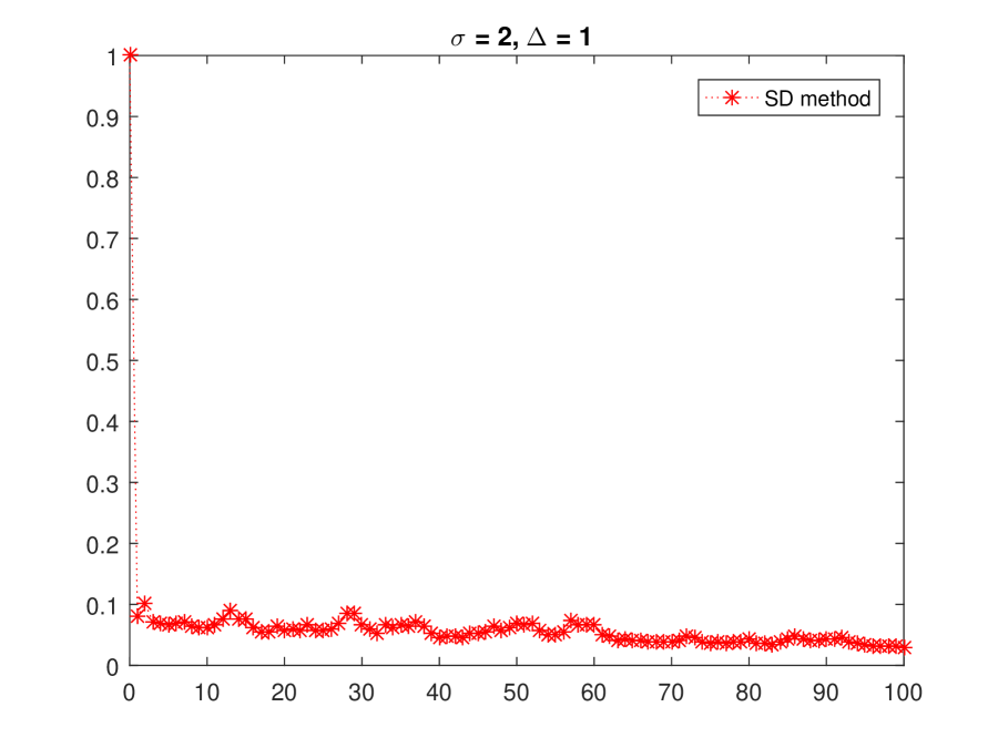
(a) Trajectory for (3.2) with $\sigma=2$.

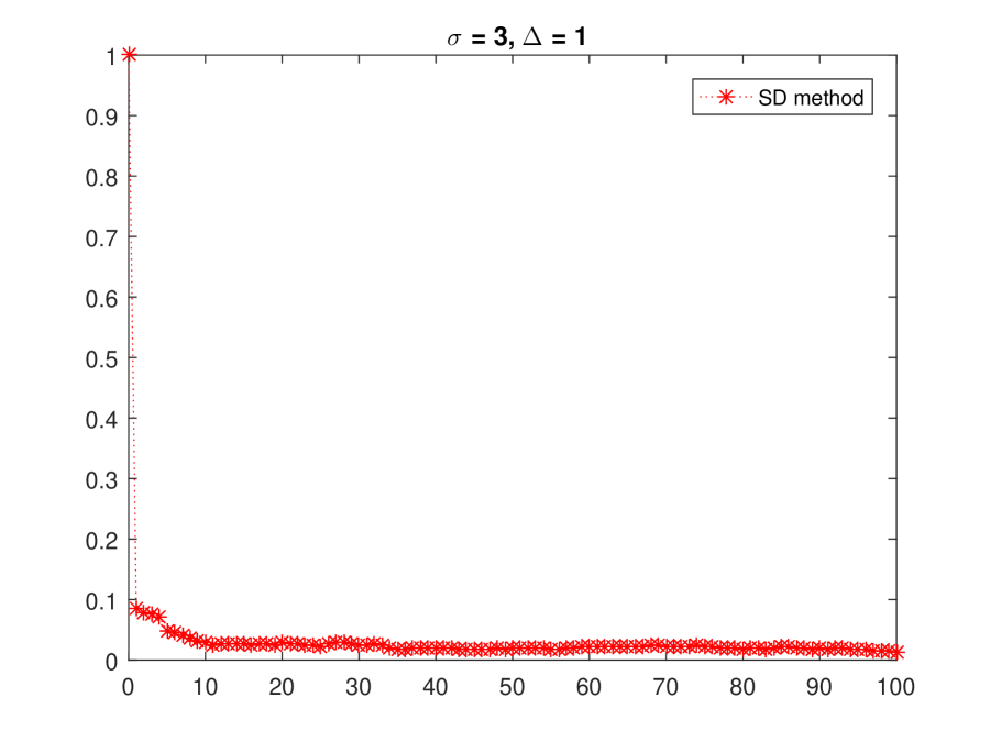
(b) Trajectory for (3.2) with $\sigma=3.$

Figure 1. Trajectories of (3.2) for different values of $\sigma$.

Figures 2 and 3 displays the case when $\gamma>1$ or $\sigma<\sqrt{2}.$ We consider the cases $\sigma=0$ and $\sigma=1$ accordingly. Now, we observe instability and an apparent finite-time explosion. The apparent explosion time in the ordinary differential equation (case $\sigma=0$) is very close to the computed one

$$\tau_{e}^{1}:=\int_{1}^{\infty}u^{-3}du=0.5,$$

and becomes closer as we lower the step-size $\Delta.$ In the case $\sigma=1$ we observe again the apparent explosion time for the SDE which is now random.

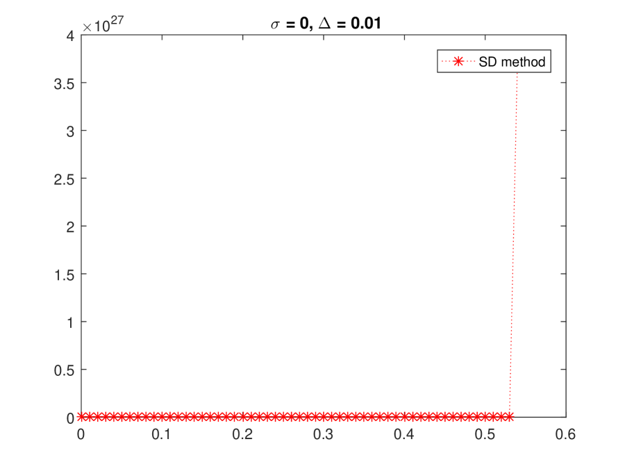
(a) Trajectory for (3.2) with $\sigma=0$ and $\Delta=0.01.$

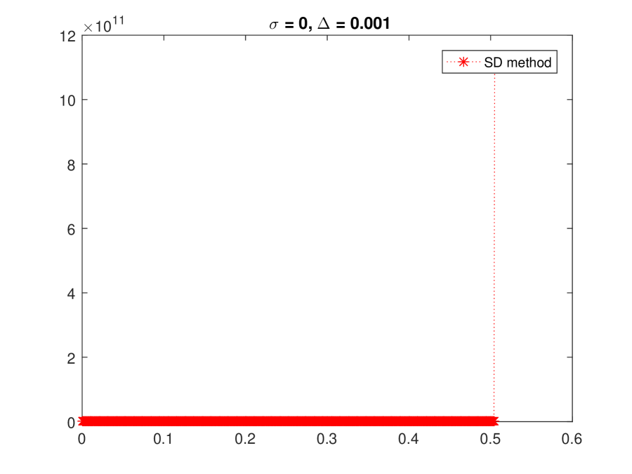
(b) Trajectory for (3.2) with $\sigma=0$ and $\Delta=0.001.$

Figure 2. Trajectories of (3.2) for $\sigma=0$ and different values of $\Delta.$.

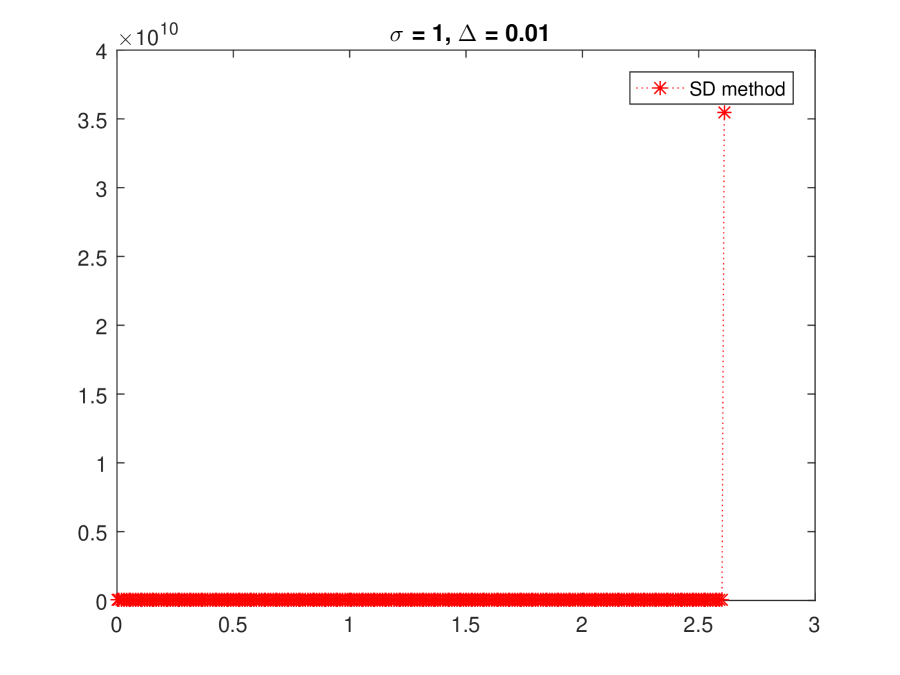
(a) Trajectory for (3.2) with $\sigma=1$ and $\Delta=0.01.$

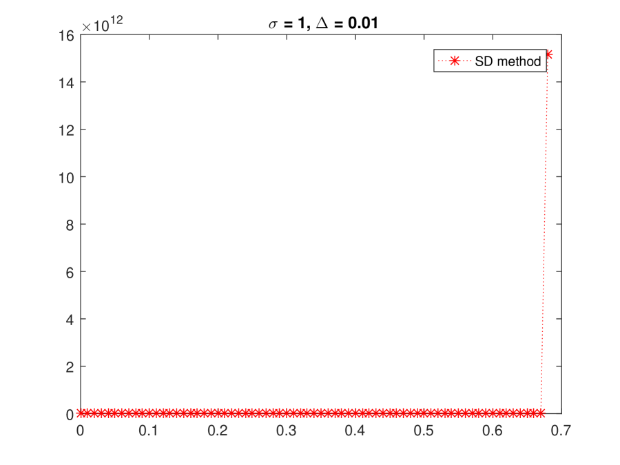
(b) Trajectory for (3.2) with $\sigma=1$ and $\Delta=0.01.$

Figure 3. Trajectories of (3.2) for $\sigma=1.$

4. Proofs

In this section we first discuss about the derivation of the semi-discrete scheme (1.2) and then we provide the proofs of Theorems 2 and 2.

Given the equidistant partition $0=t_{0}<t_{1}<\ldots<t_{N}=T$ with step size $\Delta=T/N$ we consider the following process

(4.1) $$y_{t}=y_{t_{n}}+\int_{t_{n}}^{t}\underbrace{a(y_{t_{n}})y_{s}}_{f(y_{t_{n}},y_{s})}ds+\int_{t_{n}}^{t}\underbrace{b(y_{t_{n}})y_{s}}_{g(y_{t_{n}},y_{s})}dW_{s},$$

in each subinterval $[t_{n},t_{n+1}],$ with $y_{0}=x_{0}$ a.s. By (4.1) the form of discretization becomes apparent. We discretized the drift and diffusion coefficient in a multiplicative way producing a new SDE at each subinterval with the unique strong solution

(4.2) $$y_{t}=y_{t_{n}}\exp\left\{\left(a(y_{t_{n}})-\frac{b^{2}(y_{t_{n}})}{2}\right)(t-t_{n})+b(y_{t_{n}})(W_{t}-W_{t_{n}})\right\}.$$

The first variable of the auxiliary functions $f(\cdot,\cdot)$ and $g(\cdot,\cdot)$ in (4.1) denote the discretized part. In case $a(\cdot)$ and $b(\cdot)$ are locally Lipschitz so are $f(\cdot,\cdot)$ and $g(\cdot,\cdot)$ and as a consequence we have a strong convergence result of the type (see [10, Theorem 2.1])

$$\lim_{\Delta\rightarrow 0}{\mathbb{E}}\sup_{0\leq t\leq T}|y_{t}-x_{t}|^{2}=0,$$

in the case of finite moments of the original SDE and the approximation process, that is when ${\mathbb{E}}|x_{t}|^{p}\vee{\mathbb{E}}|y_{t}|^{p}<A$ for some $p>2$ and $A>0.$ However, the strong convergence of the method does not hold in all cases considered here since the moments of $(x_{t})$ are bounded only up to an explosion time $\tau_{e}^{x_{0}}$ which may be finite in case (1.3) does not hold. The main focus here is the preservation of the dynamics in the discretization as shown in Section 3.

The stability behavior of the equilibrium solution of (1.2) is an easy task since we have an analytic expression of the solution process. Nevertheless, we discuss the steps below.

Take a $p>0$ to be specified later on and rewrite (1.2) as

$$|y_{n+1}|^{p} = |y_{n}|^{p}\exp\left\{\frac{pb^{2}(y_{n})}{2}\left(\frac{2a(y_{n})}{b^{2}(y_{n})}-1+p\right)\Delta\right\}\exp\left\{-\frac{p^{2}b^{2}(y_{n})}{2}\Delta+pb(y_{n})\Delta W_{n}\right\}$$

$$= {\mathcal{E}}(y_{n})\xi_{n+1},$$

where we used the notation $y_{n}$ for $y_{t_{n}},$ the exponential function ${\mathcal{E}}(\cdot)$ reads

$${\mathcal{E}}(u)=\exp\left\{\frac{pb^{2}(u)}{2}\left(\frac{2a(u)}{b^{2}(u)}-1+p\right)\Delta\right\}$$

and for $t\in(t_{n},t_{n+1}]$ we consider the SDE

$$d\xi_{t}=pb(y_{n})dW_{t}$$

with $\xi_{n}$=$|y_{n}|^{p}.$ Therefore ${\mathbb{E}}\xi_{n+1}$=${\mathbb{E}}|y_{n}|^{p}$ and choosing $0<p<1-\beta,$ where $\beta$ is as in Theorem 2, we get that ${\mathcal{E}}(u)\leq 1$ for any $\Delta>0$ implying on the one hand the boundness of the moments of ${y_{n}}_{n\in{\mathcal{N}}}$ and on the other hand the $p_{t}h$ moment exponential stability of the trivial solution of $y_{t}^{x_{0}}.$ This in turn implies the a.s. exponential stability of the trivial solution (see [16, Theorem 4.4.2]) and consequently (2.2). As a result we also now the rate of (2.2) which is exponential and determined by the function ${\mathcal{E}}(\cdot).$ The result of Theorem 2 follows by analogue arguments where now we consider the representation

$$|y_{n+1}|^{-p} = |y_{n}|^{-p}\exp\left\{\frac{pb^{2}(y_{n})}{2}\left(\frac{-2a(y_{n})}{b^{2}(y_{n})}+1+p\right)\Delta\right\}\exp\left\{-\frac{p^{2}b^{2}(y_{n})}{2}\Delta-pb(y_{n})\Delta W_{n}\right\}$$

$$= {\mathcal{E}}^{*}(y_{n})\xi^{*}_{n+1},$$

for $0<p<\gamma-1$ where $\gamma$ is as in the statement of Theorem 2 and

$${\mathcal{E}}^{*}(u)=\exp\left\{\frac{pb^{2}(u)}{2}\left(-\frac{2a(u)}{b^{2}(u)}+1+p\right)\Delta\right\}$$

and for $t\in(t_{n},t_{n+1}]$

$$d\xi^{*}_{t}=-pb(y_{n})dW_{t}.$$

References

- [1] M. Hutzenthaler, A. Jentzen, and P.E. Kloeden. Strong and weak divergence in finite time of Euler’s method for stochastic differential equations with non-globally Lipschitz continuous coefficients. In Proceedings of the Royal Society of London A: Mathematical, Physical and Engineering Sciences, volume 467, pages 1563–1576. The Royal Society, 2011.
- [2] M. Hutzenthaler and A. Jentzen. Numerical approximations of stochastic differential equations with non-globally Lipschitz continuous coefficients. to appear in Memoirs of the American Mathematical Society, 236(1112), 2015.
- [3] M.V. Tretyakov and Z. Zhang. A fundamental mean-square convergence theorem for SDEs with locally Lipschitz coefficients and its applications. SIAM Journal on Numerical Analysis, 51(6):3135–3162, 2013.
- [4] Sabanis S. Euler approximations with varying coefficients: the case of superlinearly growing diffusion coefficients. Annals of Applied Probability, 26(4):2083–2105, 9 2016. 19 pages.
- [5] A. Neuenkirch and L. Szpruch. First order strong approximations of scalar SDEs defined in a domain. Numerische Mathematik, 128(1):103–136, 2014.
- [6] W. Fang and M. B. Giles. Adaptive euler-maruyama method for sdes with non-globally lipschitz drift: Part i, finite time interval. arXiv preprint arXiv:1609.08101, 2016.
- [7] C. Kelly and G. Lord. Adaptive timestepping strategies for nonlinear stochastic systems. arXiv preprint arXiv:1610.04003, 2016.
- [8] C. Kelly, . Rodkina, and E. M. Rapoo. Adaptive timestepping for pathwise stability and positivity of strongly discretised nonlinear stochastic differential equations. arXiv preprint arXiv:1706.03098, 2017.
- [9] N. Halidias. Semi-discrete approximations for stochastic differential equations and applications. International Journal of Computer Mathematics, 89(6):780–794, 2012.
- [10] N. Halidias and I.S. Stamatiou. On the Numerical Solution of Some Non-Linear Stochastic Differential Equations Using the Semi-Discrete Method. Computational Methods in Applied Mathematics, 16(1):105–132, 2016.
- [11] N. Halidias. A novel approach to construct numerical methods for stochastic differential equations. Numerical Algorithms, 66(1):79–87, 2014.
- [12] Halidias N. Construction of positivity preserving numerical schemes for some multidimensional stochastic differential equations. Discrete and Continuous Dynamical Systems - Series B, 20(1):153–160, 2015.
- [13] N. Halidias. Constructing positivity preserving numerical schemes for the two-factor CIR model. Monte Carlo Methods and Applications, 21(4):313–323, 2015.
- [14] N. Halidias and I.S. Stamatiou. Approximating Explicitly the Mean-Reverting CEV Process. Journal of Probability and Statistics, Article ID 513137, 20 pages, 2015.
- [15] I.S. Stamatiou. A boundary preserving numerical scheme for the Wright-Fisher model. Journal of Computational and Applied Mathematics, DOI = 10.1016/j.cam.2017.07.011, 2017.
- [16] X. Mao. Stochastic differential equations and applications. Horwood Publishing, Chichester, 2nd edition, 2007.
- [17] John AD Appleby, Xuerong Mao, and Alexandra Rodkina. Stabilization and destabilization of nonlinear differential equations by noise. IEEE Transactions on Automatic Control, 53(3):683–691, 2008.