Impact of Beyond the Standard Model physics in the detection of the Cosmic Neutrino Background

Abstract

We discuss the effect of Beyond the Standard Model charged current interactions on the detection of the Cosmic Neutrino Background by neutrino capture on tritium in a PTOLEMY-like detector. We show that the total capture rate can be substantially modified for Dirac neutrinos if scalar or tensor right-chiral currents, with strength consistent with current experimental bounds, are at play. We find that the total capture rate for Dirac neutrinos, $\Gamma_{\rm D}^{\rm BSM}$, can be between 0.3 to 2.2 of what is expected for Dirac neutrinos in the Standard Model, $\Gamma_{\rm D}^{\rm SM}$, so that it can be made as large as the rate expected for Majorana neutrinos with only Standard Model interactions. A non-negligible primordial abundance of right-handed neutrinos can only worsen the situation, increasing $\Gamma_{\rm D}^{\rm BSM}$ by 30 to 90%. On the other hand, if a much lower total rate is measured than what is expected for $\Gamma_{\rm D}^{\rm SM}$, it may be a sign of new physics.

1 Introduction

The accidental discovery of the Cosmic Microwave Background (CMB) radiation by Penzias and Wilson in 1965 laid the foundations for the enormous progress in our understanding of the evolution of the Universe. This is the oldest directly observed radiation in the Universe, dating from the epoch of recombination, and its precise study, carried out in the last decades by various cosmological probes, lead to the establishment of the standard model of cosmology. This model also predicts the existence of a Cosmic Neutrino Background ($\rm C\nu B$), a relic radiation that decoupled from matter when the Universe was merely a second old, which is expected to have played a crucial role in primordial nucleosynthesis and in large scale structures formation.

The CMB anisotropies, an indirect imprint of the $\rm C\nu B$, have already offered two important constraints in connection to particle physics: a limit on the sum of neutrino masses and the effective number of neutrino species. A confirmation of the $\rm C\nu B$ by direct detection using experiments on Earth would not only represent a further triumph of modern cosmology, but it would also constitute an unique opportunity to probe neutrino properties. For a long time this was believed to be an impossible task since relic neutrinos are expected to be non-relativistic today with an average momentum of about $10^{-4}$ eV. Recent developments have allowed to revive the old suggestion by Weinberg Weinberg:1962zza of capturing them on $\beta$-decaying nuclei, a process with no energy threshold. In fact, a real experimental proposal, the Princeton Tritium Observatory for Light, Early-Universe, Massive-Neutrino Yield (PTOLEMY) experiment Betts:2013uya is currently assessing the prospects for using the process $\nu+\ ^{3}{\rm H}\to\ ^{3}{\rm He}+e^{-}$. The signature of $\rm C\nu B$ capture would be a peak in the final electron spectrum at an energy $2m_{\nu}$ above the $\beta$-decay endpoint. This requires a very challenging energy resolution $\lesssim 0.1$ eV for the final electrons to be distinguished from the $\beta$-decay background. This has triggered interest in the community to investigate what could potentially be learned in such experiment Long:2014zva ; Zhang:2015wua ; Chen:2015dka ; deSalas:2017wtt .

In particular, the authors of ref. Long:2014zva have shown how the direct measurement of the $\rm C\nu B$ would allow to discriminate Majorana from Dirac neutrinos, as the former would produce a capture rate twice as large as the latter. This is because for non-relativistic states chirality and helicity do not coincide, and it is helicity, not chirality, which is conserved by the $\rm C\nu B$. Their conclusions rely on the fact that only the neutrinos that interact weakly according to the Standard Model (SM) could be produced and kept in thermal equilibrium before decoupling, a feature that could be modified by new interactions or a different thermal history Zhang:2015wua ; Chen:2015dka .

In this paper we try to answer the following question: if neutrinos have new Beyond the Standard Model (BSM) interactions, how would this affect the relic neutrino detection rate in PTOLEMY-like detectors? We implement these possible deviations using an effective lagrangian approach.

We start in section 2 by describing the gauge invariant operators that we will consider and computing the rate of neutrino capture on tritium. In section 3 we introduce the experimental resolution and describe in detail when the signal from the electron produced in the capture can be distinguished from the electron produced by the $\beta$-decay background. In section 4 we discuss the experimental bounds from $\beta$-decay on the BSM physics coefficients, and we show how the capture rate is modified with respect to the standard case for various regions of the parameter space. In section 5 we discuss how gravitational clustering or a primordial abundance of right-handed neutrinos present in the $\rm C\nu B$ today would affect our results. Finally our conclusions are drawn in 6. In appendix A we discuss how the interplay between the experimental resolution and the neutrino mass ordering affect the possibility of distinguishing the electron peaks due to each neutrino mass eigenstate.

2 Effective lagrangian approach for the BSM neutrino interactions

In the SM, the weak interactions have a purely $V-A$ Lorentz structure. Since the simple fact that neutrinos have a non-zero mass constitutes already an evidence for BSM physics, we will allow here for other possibilities. This can be done in a model independent fashion using an effective field theory approach. We will consider dimension-six operators which are SU(2)${}_{L}\times$U(1)_Y invariant, but which also include right-handed neutrinos Grzadkowski:2010es ; Cirigliano:2012ab ; Cirigliano:2013xha . More precisely, we write

$$\mathscr{L}_{\rm BSM}=\mathscr{L}_{\rm SM}^{(4)}+\mathscr{L}_{m_{\nu}}+\frac{1}{\Lambda^{2}}\sum_{k=1}^{12}c_{k}^{(6)}Q_{k}^{(6)},$$ (1)

where $\mathscr{L}_{\rm SM}^{(4)}$ is the dimension-four SM lagrangian, $\mathscr{L}_{m_{\nu}}$ is the neutrino mass lagrangian, which can either come from a dimension 4 operator involving right handed neutrinos or from the dimension 5 Weinberg operator; $\Lambda$ is the maximum energy scale at which the theory is still valid; and the $c_{k}^{(6)}$ are dimensionless coupling constants. The set of operators with left- and right-handed neutrinos, $Q_{k}^{(6)}=\{Q_{k}^{(6)}(\nu_{L}),Q_{k}^{(6)}(\nu_{R})\}$, is given in table 1.

Four-fermion Operators		Vertex Corrections
$Q_{\nu_{L}}^{(6)}$	$Q_{\nu_{R}}^{(6)}$	$Q_{\Phi}^{(6)}$
$Q_{1}=(\overline{l_{L}}e_{R})(\overline{d_{R}}q_{L})$	$Q_{5}=(\overline{l_{L}}\nu_{R})\varepsilon(\overline{q_{L}}d_{R})$	$Q_{9}=i(\Phi^{T}\varepsilon D_{\mu}\Phi)(\overline{u_{R}}\gamma_{\mu}d_{R})$
$Q_{2}=(\overline{l_{L}}e_{R})\varepsilon(\overline{q_{L}}u_{R})$	$Q_{6}=(\overline{\nu_{R}}l_{L})(\overline{q_{L}}u_{R})$	$Q_{10}=i(\Phi^{T}\varepsilon D_{\mu}\Phi)(\overline{\nu_{R}}\gamma^{\mu}e_{R})$
$Q_{3}=(\overline{l_{L}}\gamma^{\mu}\tau^{A}l_{L})(\overline{q_{L}}\gamma_{\mu}\tau^{A}q_{L})$	$Q_{7}=(\overline{e_{R}}\gamma^{\mu}\nu_{R})(\overline{u_{R}}\gamma_{\mu}d_{R})$	$Q_{11}=(\Phi^{\dagger}i\overset{\text{\tiny$\longleftrightarrow$}}{D_{\mu}^{a}}\Phi)(\overline{q_{L}}\gamma_{\mu}\tau^{A}q_{L})$
$Q_{4}=(\overline{l_{L}}\sigma^{\mu\rho}e_{R})\varepsilon(\overline{q_{L}}\sigma_{\mu\rho}u_{R})$	$Q_{8}=(\overline{l_{L}}\sigma^{\mu\rho}\nu_{R})\varepsilon(\overline{q_{L}}\sigma_{\mu\rho}d_{R})$	$Q_{12}=(\Phi^{\dagger}i\overset{\text{\tiny$\longleftrightarrow$}}{D_{\mu}^{a}}\Phi)(\overline{l_{L}}\gamma^{\mu}\tau^{A}l_{L})$

Table 1: Dimension-six operators relevant for neutrino capture. Here $l_{L},q_{L}$ are the SM lepton and quark SU(2)_L doublets while $u_{R},d_{R},e_{R},\nu_{R}$ are the corresponding SM singlets. The SU(2)_L generators are denoted with $\tau^{A}$ while $\varepsilon_{ij}$ is the totally antisymmetric tensor with $\varepsilon_{12}=+1$. We do not include the invariant operator $(\overline{\nu_{R}}\sigma^{\mu\rho}l_{L})(\overline{q_{L}}\sigma_{\mu\rho}u_{R})$ in the list because it does not contribute to the relic capture.

The terms relevant for our calculation of the BSM relic neutrino capture rate on $\beta$-decaying tritium can be obtained writing eq. (1) in terms of mass eigenstates

$$\mathscr{L}_{\rm eff}=-\frac{G_{F}}{\sqrt{2}}V_{ud}\,U_{ej}\,\left\{[\bar{e}\gamma^{\mu}(1-\gamma^{5})\nu_{j}][\bar{u}\gamma_{\mu}(1-\gamma^{5})d]+\sum_{l,q}\epsilon_{lq}[\bar{e}\mathscr{O}_{l}\nu_{j}][\bar{u}\mathscr{O}_{q}d]\right\}+{\rm h.c.},$$ (2)

where a sum over the three neutrino mass eigenstates $j=1,2,3$ is implied. The couplings $\epsilon_{lq}$, related to the dimensionless couplings $c_{k}^{(6)}$ (see ref. (Cirigliano:2012ab, )), parametrize the BSM physics effects, with $l$ ($q$) labelling the Lorentz structure of the lepton (quark) current, as given by $\mathscr{O}_{l}$ ($\mathscr{O}_{q}$) in table 2. $V_{ud}$ and $U_{ej}$ correspond to the Cabibbo-Kobayashi-Maskawa (CKM) and Pontecorvo-Maki-Nakagawa-Sakata (PMNS) mixing matrices elements relevant to the process, respectively.

Equation (2) can be used to calculate the neutrino absorption on tritium

$$\nu_{j}+\ ^{3}{\rm H}\to\ ^{3}{\rm He}+e^{-}\,,$$

in the presence of BSM interactions. To this end, we need to properly define the hadronic matrix elements involving the quark current in eq. (2). Following ref. Ludl:2016ane , we have

$$\begin{aligned} \langle p(p_{p})|\bar{u}\gamma^{\mu}(1\pm\gamma^{5})d|n(p_{n})\rangle&=\overline{u_{p}}(p_{p})\gamma^{\mu}[g_{V}(q^{2})\pm g_{A}(q^{2})\gamma^{5}]u_{n}(p_{n}),\\ \langle p(p_{p})|\bar{u}d|n(p_{n})\rangle&=g_{S}(q^{2})\,\overline{u_{p}}(p_{p})\,u_{n}(p_{n}),\\ \langle p(p_{p})|\bar{u}\gamma^{5}d|n(p_{n})\rangle&=g_{P}(q^{2})\,\overline{u_{p}}(p_{p})\gamma^{5}u_{n}(p_{n}),\\ \langle p(p_{p})|\bar{u}\sigma^{\mu\nu}(1\pm\gamma^{5})d|n(p_{n})\rangle&=g_{T}(q^{2})\,\overline{u_{p}}(p_{p})\sigma^{\mu\nu}(1\pm\gamma^{5})u_{n}(p_{n}).\end{aligned}$$ (3)

We have introduced the hadronic form factors $g_{h}(q^{2})$, with $h=V,A,S,P,T$ corresponding to the vector, axial, scalar, pseudoscalar and tensor Lorentz structures, respectively. Although these form factors depend on the transferred momentum $q^{2}=(p_{n}-p_{p})^{2}$, for the capture rate we are only interested in the $q^{2}\simeq 0$ limit. In our numerical analysis we will use the values shown in table 3 Akulov:2002gh ; Gonzalez-Alonso:2013ura ; Bhattacharya:2015esa .

$\epsilon_{lq}$	$\mathscr{O}_{l}$	$\mathscr{O}_{q}$
$\epsilon_{LL}$	$\gamma^{\mu}(1-\gamma^{5})$	$\gamma_{\mu}(1-\gamma^{5})$
$\epsilon_{LR}$	$\gamma^{\mu}(1-\gamma^{5})$	$\gamma_{\mu}(1+\gamma^{5})$
$\epsilon_{RL}$	$\gamma^{\mu}(1+\gamma^{5})$	$\gamma_{\mu}(1-\gamma^{5})$
$\epsilon_{RR}$	$\gamma^{\mu}(1+\gamma^{5})$	$\gamma_{\mu}(1+\gamma^{5})$
$\epsilon_{LS}$	$1-\gamma^{5}$	$1$
$\epsilon_{RS}$	$1+\gamma^{5}$	$1$
$\epsilon_{LP}$	$1-\gamma^{5}$	$-\gamma^{5}$
$\epsilon_{RP}$	$1+\gamma^{5}$	$-\gamma^{5}$
$\epsilon_{LT}$	$\sigma^{\mu\nu}(1-\gamma^{5})$	$\sigma_{\mu\nu}(1-\gamma^{5})$
$\epsilon_{RT}$	$\sigma^{\mu\nu}(1+\gamma^{5})$	$\sigma_{\mu\nu}(1+\gamma^{5})$

Table 2: Parameters and their corresponding Lorentz structures for the BSM currents considered in this work.

Following the calculation of ref. Long:2014zva , the capture cross section for a neutrino mass eigenstate $j$, with helicity $h_{j}=\pm 1$ and velocity $v_{j}$ including BSM effects is given by

$$\sigma_{j}^{\rm BSM}(h_{j})v_{j}=\frac{G_{F}^{2}}{2\pi}\left|V_{ud}\right|^{2}\left|U_{ej}\right|^{2}F_{Z}(E_{e})\,\frac{m_{\rm{}^{3}He}}{m_{\rm{}^{3}H}}E_{e}\,p_{e}\,T_{j}(h_{j},\epsilon_{lq}),$$ (4)

where $m_{\rm{}^{3}He}$ and $m_{\rm{}^{3}H}$ are the helium and tritium masses, and $E_{e}$, $m_{e}$, $p_{e}$ are the electron energy, mass and momentum, respectively. The $T_{j}(h_{j},\epsilon_{lq})$ function contains the dependence on the neutrino helicity and on the $\epsilon_{lq}$ parameters,

$$T_{j}(h_{j},\epsilon_{lq}) ={\cal A}(h_{j})\left[g_{V}^{2}\left(\epsilon_{LL}+\epsilon_{LR}+1\right)^{2}+3\,g_{A}^{2}\left(\epsilon_{LL}-\epsilon_{LR}+1\right)^{2}+g_{S}^{2}\,\epsilon_{LS}^{2}+48\,g_{T}^{2}\,\epsilon_{LT}^{2}\right.$$

$$\qquad\qquad\left.+\frac{2m_{e}}{E_{e}}\,[g_{S}\,g_{V}\,\epsilon_{LS}\left(\epsilon_{LL}+\epsilon_{LR}+1\right)-12\,g_{A}\,g_{T}\,\epsilon_{LT}\left(\epsilon_{LL}-\epsilon_{LR}+1\right)]\right]$$

$$\quad+{\cal A}(-h_{j})\left[g_{V}^{2}\,(\epsilon_{RR}+\epsilon_{RL})^{2}+3\,g_{A}^{2}\,(\epsilon_{RR}-\epsilon_{RL})^{2}+g_{S}^{2}\,\epsilon_{RS}^{2}+48\,g_{T}^{2}\,\epsilon_{RT}^{2}\right.$$

$$\qquad\qquad\qquad\left.+\frac{2m_{e}}{E_{e}}\,[g_{S}\,g_{V}\,\epsilon_{RS}\,(\epsilon_{RR}+\epsilon_{RL})\,-12\,g_{A}\,g_{T}\,\epsilon_{RT}\,(\epsilon_{RR}-\epsilon_{RL})]\right]$$

$$\quad+2\,\frac{m_{j}}{E_{j}}\left\{g_{S}\,g_{V}\,\epsilon_{RS}\,\left(\epsilon_{LL}+\epsilon_{LR}+1\right)+\epsilon_{LS}\,(\epsilon_{RR}+\epsilon_{RL}))\right.$$

$$\qquad\qquad\ \left.-12\,g_{A}\,g_{T}(\epsilon_{RT}\,\left(\epsilon_{LL}-\epsilon_{LR}+1\right)+\epsilon_{LT}\,(\epsilon_{RR}-\epsilon_{RL}))\right\}$$

$$\quad+2\,\frac{m_{j}m_{e}}{E_{j}E_{e}}\left\{g_{V}^{2}\,(\epsilon_{LL}+\epsilon_{LR}+1)(\epsilon_{RR}+\epsilon_{RL})+3\,g_{A}^{2}\,(\epsilon_{LL}-\epsilon_{LR}+1)(\epsilon_{RR}-\epsilon_{RL})\right.$$

$$\qquad\qquad\qquad\left.+g_{S}^{2}\,\epsilon_{RS}\,\epsilon_{LS}+48\,g_{T}^{2}\,\epsilon_{RT}\,\epsilon_{LT}\right\},$$ (5)

with $m_{j},E_{j}$ the mass and energy of the $j$-th neutrino mass eigenstate and ${\cal A}(h_{j})=1-2h_{j}v_{j}$. Let us note that ${\cal A}(h_{j})\simeq 1$ for non-relativistic neutrinos, corresponding to the case on which we will focus in section 3. Furthermore, notice that the capture rate is independent of the pseudoscalar couplings $\epsilon_{lP}$. The Fermi function $F_{Z}(E_{e})$, which takes cares of the enhancement of the cross section due to the Coulomb attraction between the proton and electron, is given by

$$F_{Z}(E_{e})=\frac{2\pi Z\alpha E_{e}}{p_{e}\left[1-e^{\frac{-2\pi Z\alpha E_{e}}{p_{e}}}\right]}\,.$$ (6)

Summing over all the neutrino mass eigenstates, one can calculate the total $\rm{}^{3}H$ capture rate

$$\Gamma_{\rm C\nu B}^{\rm BSM}=N_{T}\sum_{j=1}^{3}\,\Gamma_{\rm C\nu B}^{\rm BSM}(j)=N_{T}\sum_{j=1}^{3}\,\left[\sigma_{j}^{\rm BSM}(+1)\,v_{j}\,n_{\nu_{+}^{j}}+\sigma_{j}^{\rm BSM}(-1)\,v_{j}\,n_{\nu_{-}^{j}}\right],$$ (7)

where $N_{T}$ is the number of nuclei present in the sample and $n_{\nu_{\pm}^{j}}$ the number density at the present time of the helical state $\nu_{\pm}^{j}$.

Form Factor	Value	Reference
$g_{V}(0)$	$1$	Gershtein:1955fb ; Feynman:1958ty
$g_{A}(0)/g_{V}(0)$	$1.2646\pm 0.0035$	Akulov:2002gh
$g_{S}(0)$	$1.02\pm 0.11$	Gonzalez-Alonso:2013ura
$g_{P}(0)$	$349\pm 9$	Gonzalez-Alonso:2013ura
$g_{T}(0)$	$1.020\pm 0.076$	Bhattacharya:2015esa

Table 3: Hadronic form factors considered in this work.

3 Detection of the $\rm C\nu B$ by a PTOLEMY-like detector

A PTOLEMY-like experiment Betts:2013uya aims to detect the $\rm C\nu B$ through the neutrino capture by tritium, a reaction that has no energy threshold. We can safely assume that $\rm C\nu B$ neutrinos are non-relativistic today as their root mean momentum is $\langle p\rangle\approx 0.6\ {\rm meV}\ll m_{j}$ Weinberg:1962zza . This has two crucial consequences. First, the neutrino flavour eigenstates have suffered decoherence into their mass eigenstates, so a detector would, in fact, measure the contribution of each neutrino mass eigenstate. Second, at the time of the creation of the $\rm C\nu B$, i.e. when neutrinos decoupled from the primordial plasma, they were ultrarelativistic, making chiral and helical eigenstates effectively equal. However, as neutrinos evolved into a non-relativistic state due to the expansion of the Universe, chirality and helicity became different. Since neutrinos were free streaming, it was helicity, not chirality, that was conserved in the process. This implies that the neutrino number density is $n_{\nu_{+}^{j}}=n_{\nu_{-}^{j}}=n_{0}\approx 56$ cm^-3 in the Majorana case, while $n_{\nu_{-}^{j}}=n_{0}$ and $n_{\nu_{+}^{j}}=0$ in the Dirac case. If no BSM interactions are present, the function $T_{j}(h_{j},\epsilon_{lq})$ reduces to

$$T_{j}(h_{j},0) ={\cal A}(h_{j})\left[g_{V}^{2}+3\,g_{A}^{2}\right],$$

from which, using eq. (7), we conclude that

$$\Gamma^{\rm M}_{\rm C\nu B}=2\,\Gamma^{\rm D}_{\rm C\nu B}=85.7\;\rm[kg\,yr]^{-1}\,,$$ (8)

where $\Gamma^{\rm M}_{\rm C\nu B}$ and $\Gamma^{\rm D}_{\rm C\nu B}$ are the Majorana and Dirac capture rates. We will consider in section 5 the modifications to the neutrino abundance due to BSM physics.

The signature of relic neutrinos in a PTOLEMY-like detector is given by the electron created in the capture process. Nonetheless, tritium can also undergo $\beta$-decay, giving rise to a continuous electron spectrum. As a consequence, one needs to discriminate the electrons produced by the $\rm C\nu B$ neutrino capture from the electrons produced by $\beta$-decays. Using kinematics, the electrons produced by the $\nu_{j}$ relic neutrinos capture will have a definite energy Long:2014zva

$$E_{e}^{{\rm C\nu B},j}\simeq m_{e}+K_{\rm end}^{0}+2\,m_{j},$$ (9)

where $K_{\rm end}^{0}$ corresponds to the $\beta$-decay endpoint energy. This implies that relic neutrinos could produce one or more peaks in the electron energy spectrum at energies larger than the endpoint one. If so, $\rm C\nu B$ and $\beta$-decay events can in principle be discriminated from each other. It is clear that the finite energy resolution of the real detector plays an essential role in establishing whether the two signals can be separated or not. In order to estimate the signal in a more realistic way we will follow Long:2014zva and convolute the $\rm C\nu B$ capture rate of eq. (7) and the $\beta$-decay background with a Gaussian function

$$\frac{d\Gamma_{\rm C\nu B}^{\rm BSM}}{dE_{e}} =\frac{1}{\sqrt{2\pi\sigma^{2}}}\sum_{j=1}^{3}\int_{-\infty}^{\infty}\,dE_{e}^{\prime}\,\Gamma_{\rm C\nu B}^{\rm BSM}(j)\,\exp\left[-\frac{(E_{e}^{\prime}-E_{e})^{2}}{2\sigma^{2}}\right]\,\delta(E_{e}-E_{e}^{{\rm C\nu B},j}),$$ (10a)

$$\frac{d\Gamma_{\beta}}{dE_{e}} =\frac{1}{\sqrt{2\pi\sigma^{2}}}\int_{-\infty}^{\infty}\,dE_{e}^{\prime}\,\frac{d\Gamma_{\beta}}{dE_{e}^{\prime}}\,\exp\left[-\frac{(E_{e}^{\prime}-E_{e})^{2}}{2\sigma^{2}}\right],$$ (10b)

where $\sigma$ is the expected experimental energy resolution. The complete expression for the $\beta$-decay rate $\displaystyle\frac{d\Gamma_{\beta}}{dE_{e}^{\prime}}$ can be found in ref. Ludl:2016ane .

In order to estimate the total number of events produced by the $\rm C\nu B$ and $\beta$-decay in the region in which we expect a $\rm C\nu B$ signal, we define the full width at half maximum (FWHM) of the Gaussian function as $\Delta=\sqrt{8\ln 2}\,\sigma$. With this definition, we have

$${\cal N}_{\rm C\nu B}^{\rm BSM}(\Delta) =\int_{E_{e}^{\rm C\nu B}-\Delta/2}^{E_{e}^{\rm C\nu B}+\Delta/2}\,dE_{e}\frac{d\Gamma_{\rm C\nu B}^{\rm BSM}}{dE_{e}},$$ (11a)

$${\cal N}_{\beta}(\Delta) =\int_{E_{e}^{\rm C\nu B}-\Delta/2}^{E_{e}^{\rm C\nu B}+\Delta/2}\,dE_{e}\frac{d\Gamma_{\beta}}{dE_{e}},$$ (11b)

which can be used to define the ratio

$$r_{\rm C\nu B}=\frac{{\cal N}_{\rm C\nu B}^{\rm BSM}(\Delta)}{\sqrt{{\cal N}_{\beta}(\Delta)}}.$$ (12)

We will consider that the signal can be discriminated from the background when $r_{\rm C\nu B}\geq 5$. The future PTOLEMY experiment is expected to have $\Delta=0.15$ eV Betts:2013uya in such a way that a single peak is expected if the sum of the neutrino masses is about $0.1$ eV. For smaller masses, a smaller value of $\Delta$ would be needed to discriminate the signal from the background. We study more in detail the interplay between $\Delta$, neutrino masses and the position of the peaks observed at PTOLEMY-like detectors in Appendix A.

4 On the contributions of BSM physics to $\rm C\nu B$ capture rate

The BSM lagrangian of eq. (2) generates not only new contributions to the neutrino capture by tritium, but also modifies other low energy processes. To assess the size of the modification to the neutrino $\rm C\nu B$ capture rate, we first need to take into account the experimental bounds on the $\epsilon_{lq}$ coefficients. Limits from Cabbibo Universality Hardy:2008gy , radiative pion decay Mateu:2007tr and neutron decays Bhattacharya:2011qm put bounds on the $\epsilon_{Lq}$ left-chiral couplings; meanwhile, limits coming from the $\beta$-decay of several nuclei have been reviewed in ref. Severijns:2006dr . A complete compendium of the limits regarding low energy decays is given in refs. Cirigliano:2012ab ; Cirigliano:2013xha . For our purposes, we will consider the cases considered in ref. Severijns:2006dr , as they include couplings with right-handed neutrinos. The constraints are given in terms of the following combinations of couplings:

$$\begin{aligned} C_{V}&=g_{V}(1+\epsilon_{LL}+\epsilon_{LR}+\epsilon_{RL}+\epsilon_{RR}),&C_{V}^{\prime}&=g_{V}(1+\epsilon_{LL}+\epsilon_{LR}-\epsilon_{RL}-\epsilon_{RR}),\\ C_{A}&=-g_{A}(1+\epsilon_{LL}-\epsilon_{LR}-\epsilon_{RL}+\epsilon_{RR}),&C_{A}^{\prime}&=-g_{A}(1+\epsilon_{LL}-\epsilon_{LR}+\epsilon_{RL}-\epsilon_{RR}),\\ C_{S}&=g_{S}(\epsilon_{LS}+\epsilon_{RS}),&C_{S}^{\prime}&=g_{S}(\epsilon_{LS}-\epsilon_{RS}),\\ C_{T}&=4\,g_{T}(\epsilon_{LT}+\epsilon_{RT}),&C_{T}^{\prime}&=4\,g_{T}(\epsilon_{LT}-\epsilon_{RT}).\end{aligned}$$ (13)

Accordingly, we need to convert the bounds on the $C_{i}^{(\prime)}$ into bounds on $\epsilon_{lq}$ at 3$\sigma$ C.L. To this end, we have performed a scan over the ranges

$$\begin{aligned} -10^{-3}\leq&\epsilon_{LL}\leq 10^{-3}\,,&-10^{-3}\leq&\epsilon_{LR}\leq 10^{-3}\,,\\ -2.8\times 10^{-3}\leq&\epsilon_{LS}\leq 5\times 10^{-3}\,,&-2\times 10^{-3}\leq&\epsilon_{LT}\leq 2.1\times 10^{-3}\,,\\ \end{aligned}$$ (14)

and

$$\left|\epsilon_{Rq}\right|\leq 10^{-1},$$ (15)

keeping only the points consistent with each of the allowed regions of the $C_{h}^{(\prime)}$ in ref. Severijns:2006dr . Let us notice that, to translate the limits into contraints on the $\epsilon_{lq}$ parameters, we also scanned over the $g_{A}(0)/g_{V}(0)$ value given in table 3 since such parameter is affected by the presence of BSM Gonzalez-Alonso:2013uqa . The ranges in which the scan is performed have been chosen to include the constraints of refs. Hardy:2008gy ; Mateu:2007tr ; Bhattacharya:2011qm in the left-chiral coefficients at the 3$\sigma$ level. Although stronger limits can be imposed on right-handed couplings using pion decay Campbell:2003ir , we will not include them as they are strongly dependent on the flavour structure of the model (Cirigliano:2012ab, ; Cirigliano:2013xha, ). Finally, LHC bounds coming from $pp\to e+X+\not{E}_{T}$ have been studied in refs. Bhattacharya:2011qm ; Cirigliano:2012ab . However, the analysis is performed supposing the interactions of eq. (2) remain pointlike up to the LHC energies, i.e. up to a few TeV. To allow for the possibility that BSM physics appears just above the electroweak scale, in our analysis we will use only the bounds coming from low energy experiments.

We found that the parameters $\epsilon_{LL}$ and $\epsilon_{LR}$ are unconstrained by the experimental data as it has been previously noted in ref. Gonzalez-Alonso:2013uqa . For reference we summarize here the bounds without the correlations — which have been included in our numerical analysis — :

1. Only left-chiral couplings allowed in the fit ($\epsilon_{Rq}=0$). The scalar and tensor terms have distinct dependence on the electron energy and mass, because of the different Lorentz structure. Computing the total capture rate $\Gamma_{\rm C\nu B}^{BSM}$ using the points that pass the low energy experimental constraints, we find

   $$0.985\,\Gamma_{\rm C\nu B}^{\rm D}\lesssim\Gamma_{\rm C\nu B}^{\rm BSM}\lesssim 1.02\,\Gamma_{\rm C\nu B}^{\rm D},$$

   where $\Gamma_{\rm C\nu B}^{D}$ is the capture rate for Dirac neutrinos with only SM interactions.

2. Only vector-axial-vector couplings allowed in the fit ($\epsilon_{LS}=\epsilon_{RS}=\epsilon_{LT}=\epsilon_{RT}=0$): in this case we get $|\epsilon_{RL}|\lesssim 8\times 10^{-2}$ and $|\epsilon_{RR}|\lesssim 5\times 10^{-2}$ at 3$\sigma$ level. Let us notice that the term linear in the right-handed couplings in eq. (2) is proportional to $m_{j}/E_{j}$, so it would be negligible for an ultrarelativistic neutrino. This term comes from the interference of the SM contribution with the right-handed neutrino current. The terms proportional to $(\epsilon_{RR}\pm\epsilon_{RL})^{2}$ come from the square of the right-handed currents, and are proportional to ${\cal A}(-h_{j})$. Using the experimentally allowed range for $\epsilon_{RR,RL}$, we find

   $$0.89\,\Gamma_{\rm C\nu B}^{\rm D}\lesssim\Gamma_{\rm C\nu B}^{\rm BSM}\lesssim 1.11\,\Gamma_{\rm C\nu B}^{\rm D}.$$

   

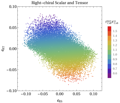
   Figure 1: Ratio between the BSM capture rate for the right-chiral scalar and tensor couplings scenario with respect to the SM Dirac case in the plane $(\epsilon_{RS}$ versus $\epsilon_{RT})$. We use a color code to indicate the range of values of the ratio.

3. Only right-chiral scalar and tensor couplings allowed in the fit ($\epsilon_{LS}=\epsilon_{LT}=\epsilon_{RL}=\epsilon_{RR}=0$): in this case we get $|\epsilon_{RS}|\lesssim 1.1\times 10^{-1}$ and $|\epsilon_{RT}|\lesssim 8\times 10^{-2}$ at $3\sigma$. Again the term proportional to the neutrino mass comes from the interference between SM and right-handed currents. Furthermore, we observe that this interference term does not depend on the neutrino helicity. This is due to the different Lorentz structures that appear in the BSM lagrangian. Considering the allowed parameter space, we find

   $$0.61\,\Gamma_{\rm C\nu B}^{\rm D}\lesssim\Gamma_{\rm C\nu B}^{\rm BSM}\lesssim 1.52\,\Gamma_{\rm C\nu B}^{\rm D}.$$

   Since in this case the parameter space is highly correlated due to the correlations coming from the $\beta$-decay bounds, we show in figure 1 the rate between the BSM capture rate and the SM Dirac case in the $(\epsilon_{RS},\epsilon_{RT})$ plane.

4. Five free couplings allowed in the fit: in this case we get $|\epsilon_{RS}|\lesssim 10^{-1}$ and $|\epsilon_{RT}|\lesssim 8\times 10^{-2}$ at $3\sigma$. Here the interference term proportional to the neutrino mass depends on the product between $\epsilon_{LS,LT}$ and $\epsilon_{RS,RT}$. We show in figure 2 the ratio between the BSM capture rate and the SM Dirac rate in the $(\epsilon_{RS},\epsilon_{RT})$ plane, in which we find the strongest correlation between the couplings. We find that the ratio can be at the most 2.2 times the SM one, which is interesting as in this case Dirac neutrinos with BSM interactions can mimic Majorana neutrinos in the SM. However, there are regions in parameter space in which the rate is considerably lower than the SM one.

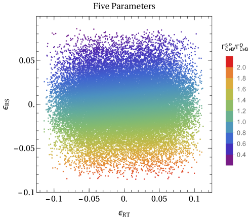
Figure 2: Ratio between the BSM capture rate with respect to the SM Dirac case for the five free couplings scenario in the plane $(\epsilon_{RS}$ versus $\epsilon_{RT})$. The maximum (minimum) value of the ratio is 2.2 (0.3).

Let us conclude stressing that pure Majorana neutrinos fall in the “only left-chiral couplings” category (case 1 above), with only a small modification of order $2\%$ allowed in the capture rate. Dirac neutrinos have instead a much richer phenomenology, with all the above cases possible (depending on the gauge invariant operators of table 1 generated in the UV theory). On the other hand, one could also worry about possible modifications of the tritium $\beta$-decay spectrum generated by BSM interactions, which could make the $\rm C\nu B$ detection more involved. Nevertheless, it has been shown in ref. (Ludl:2016ane, ) that the endpoint of the $\beta$-decay spectrum is not significantly modified by BSM physics; thus, in principle, relic neutrino detection would be still possible in this case.

5 On the relic right-handed neutrino abundance

As we have seen in section 3, without BSM contributions the neutrino number density today is expected to be

$$\begin{aligned} n_{\nu_{-}^{j}}&=n_{0},&n_{\nu_{+}^{j}}&=n_{0}&&{\rm(Majorana)},\\ n_{\nu_{-}^{j}}&=n_{0},&n_{\nu_{+}^{j}}&=0&&{\rm(Dirac)},\end{aligned}$$ (16)

with the capture rate in both cases given in eq. (8). There are three ways in which this result can be modified: (i) if neutrinos underwent a gravitational clustering process, (ii) if BSM interactions are present, and (iii) if an initial abundance of right-handed neutrinos was present in the early universe.

Neutrino motion in the Dark Matter gravitational potential has the effect of modifying the direction of the neutrino momentum without affecting its spin Duda:2001hd . The immediate consequence is that neutrinos undergo a process of gravitational clustering that tends to equilibrate the $h_{j}=+1$ and $h_{j}=-1$ populations. Since for Majorana neutrinos there is already equilibrium, eq. (16) is still valid. The situation is different for Dirac neutrinos, for which we get

$$n_{\nu_{-}^{j}} =n_{0}/2, n_{\nu_{+}^{j}} =n_{0}/2 {\rm(Dirac,\,clustering)}.$$ (17)

Nevertheless, eq. (8) is still valid since the additional right-handed neutrino population in the Dirac case with clustering compensates for the loss in the left-handed neutrino population. Very recently, an N-body simulation has been considered in ref. deSalas:2017wtt to estimate the relic neutrino density enhancement on Earth. The main result is that the clustering effect is negligible in the minimal Normal Ordering case while, for minimal Inverted Ordering, the capture rate can be increased up to 20% for both Dirac and Majorana neutrinos.

We now turn to the case in which BSM interactions are present. Since BSM physics modify the electroweak rates, this could potentially affect the left-handed neutrino abundance. As we have seen in section 4, we must have at most $\epsilon_{lq}\lesssim 10^{-1}$ to be compatible with $\beta$-decay and other low energy experimental bounds (with many parameters much smaller). As such, the active neutrinos were maintained in equilibrium with the plasma mainly by SM interactions, and we do not expect a significant change in the left-handed neutrino number density $n_{\nu_{+}^{j}}$.

Let us finally consider the case in which an initial abundance of right-handed neutrinos is present. Such abundance can be either thermal or non-thermal. A thermal population can be achieved by non-standard interactions or in the presence of a tiny neutrino magnetic moment Anchordoqui:2012qu ; SolagurenBeascoa:2012cz ; Zhang:2015wua . Following Zhang:2015wua , when the expansion of Universe becomes faster than the interaction rate, the right-handed neutrinos decouple as usual. At this freeze out temperature, $T_{R}$, the number densities of left- and right-handed neutrinos must be equal

$$n_{\nu_{R}^{j}}(T_{R})=n_{\nu_{L}^{j}}(T_{R}).$$ (18)

Using entropy conservation, we can relate the right-handed neutrino abundance at late times with the left-handed abundance, obtaining Zhang:2015wua

$$\frac{n_{\nu_{R}^{j}}(T_{\nu})}{n_{\nu_{R}^{j}}(T_{R})}=\frac{g_{*S}(T_{\nu})}{g_{*S}(T_{R})}\left(\frac{T_{\nu}}{T_{R}}\right)^{3},$$ (19)

where $g_{*S}(T)$ is the number of relativistic degree of freedom in entropy at the temperature $T$. Choosing $T_{\nu}$ in eq. (19) to be the left-handed neutrino decoupling temperature, and using the definition of the effective number of thermal neutrino species $N_{\rm eff}$, one obtains Anchordoqui:2012qu ; SolagurenBeascoa:2012cz ; Zhang:2015wua

$$n_{\nu_{R}^{j}}(T_{\nu})=\left(\frac{1}{3}\Delta N_{\rm eff}\right)^{\frac{3}{4}}n_{\nu_{L}^{j}}(T_{\nu}),$$ (20)

where $\Delta N_{\rm eff}=N_{\rm eff}^{\rm exp}-3.046$ and $N_{\rm eff}=3.046$ is the SM value with 3 left-handed neutrinos. The experimental determination of $N_{\rm eff}$ by the Planck collaboration gives Ade:2015xua

$$N_{\rm eff}^{\rm exp}=3.14^{+0.44}_{-0.43}\qquad\text{He + Planck TT + low P + BAO}\qquad\text{at $95\%$ C.L.}$$

Combining eq. (20) with the experimental result, we get that the maximum density of right-handed neutrinos is Zhang:2015wua

$$n_{\nu_{+}^{j}} =n_{(\nu_{-}^{j})^{c}}=n_{0}^{R}\simeq 16\ {\rm cm}^{-3}.$$ (21)

The relic population of RH neutrinos modifies eq. (8) even for vanishing non-standard interactions. In the pure SM case, since the capture rate is proportional to ${\cal A}(h_{j})=1$ for both left- and right-handed neutrinos, we can have an increase in $\Gamma_{\rm C\nu B}^{\rm D}$ up to $28\%$ Zhang:2015wua . The difference is even larger if BSM interactions are turned on, although it depends crucially on the case considered. For instance, in the vector-axial-vector scenario, the capture rate is increased by roughly $30\%$, while in the five parameter scenario the increase can be up to $70\%$. In this case, we have that the $\rm C\nu B$ rate can be as large as $2.8\,\Gamma_{\rm C\nu B}^{\rm D}$, reinforcing our results on the possibility of having Dirac neutrinos with a relic capture rate numerically similar to the Majorana one.

The last possibility consists in having an initial non-thermal right-handed neutrino abundance. Following Chen:2015dka , we will suppose that right-handed Dirac neutrinos initially form a degenerated Fermi gas, decoupled from the thermal bath. In this case, the right-handed neutrino density is related to the photon density $n_{\gamma}$ by

$$n_{\nu_{R}^{j}}(T_{\gamma})=\frac{1}{6\zeta(3)}\frac{g_{*S}(T_{\gamma})}{g_{*S}(T_{R})}\vartheta\,n_{\gamma},$$ (22)

where $\vartheta=\varepsilon_{F}/T_{R}$, $\varepsilon_{F}$ the Fermi energy and $T_{R}$ the freeze out temperature of the right-handed neutrinos. The experimental limit on $\vartheta$ obtained using Planck data is $\vartheta\lesssim 3.26$, from which we get that the maximum right-handed neutrino density is Chen:2015dka

$$n_{\nu_{+}^{j}} =n_{(\nu^{j}_{-})^{c}}\simeq 36\ {\rm cm}^{-3}.$$ (23)

Since in this case we can have a larger right-handed neutrino population with respect to the thermal case, we expect larger modification in the capture rate. In the vector-axial-vector BSM case we find that the rate is increased between $40$ and $90\%$, getting closer to the value expected for Majorana neutrinos in the SM. For the other three scenarios we found larger modifications. In the right-handed scalar-tensor case, the BSM capture rate has a maximum value of about $2.5\,\Gamma_{\rm C\nu B}^{\rm D}$, while in the five-parameter case we obtain $3.5\,\Gamma_{\rm C\nu B}^{\rm D}$. We conclude noticing that, in all the cases in which a right-handed neutrino population (either thermal or non-thermal) is present, the increase in the number of neutrinos lead to an increase in the capture rate.

6 Conclusions

The detection of the $\rm C\nu B$ would be a milestone for both particle physics and cosmology. Experiments using the neutrino capture in tritium are in development, so that the detection of the $\rm C\nu B$ may become a reality in the near future. In this paper we have studied how the capture rate is modified if new interactions involving neutrinos are present. For definitiveness, we have focused on the interactions arising from generic BSM physics, including all the dimension-six operators that can modify the process $\nu+n\to e+p$. Once the experimental limits coming from low energy processes are considered, we have seen that for Majorana neutrinos the modifications to the capture rate are modest (of ${\cal O}(2\%)$), while for Dirac neutrinos we can have much larger modifications, which can either increase or diminish the capture rate up to roughly a factor of two. Since in the SM case we expect the capture rate for Majorana neutrinos to be twice the one for Dirac neutrinos, we see that the measurement of the capture rate at future experiments will not be conclusive about the Majorana or Dirac nature of neutrinos.

Another situation in which the observed neutrino capture rate can be different from the standard one is the existence of a non negligible cosmic population of right handed neutrinos. In this case the capture rate can either be left unaltered or increase (depending on the physical origin of the right handed population). This allows us to conclude that if a PTOLEMY-like experiment detects a capture rate smaller than the standard capture rate for Dirac neutrinos, it would unavoidably point to the presence of New Physics in the neutrino sector (since, as shown in section 4, the capture rate can be decreased in this case). If instead the measured capture rate is between the standard Dirac and Majorana case, or even above the standard Majorana case, the situation will not be clear, since the effect can be caused by Dirac neutrinos with either BSM interactions or an additional cosmological abundance of right-handed neutrinos. On the other hand, we have seen how important the right-chiral couplings are for the relic neutrino capture rate. Since the rate depends on $\epsilon_{Rq}$ when $m_{j}/E_{j}$ is not negligible, a possible detection of the $\rm C\nu B$ can put stronger limits on the $\epsilon_{Rq}$ couplings that other low energy processes can not.

Finally, we have also briefly discussed in appendix A the problem of distinguishing the electron peaks generated by neutrino capture and $\beta$-decay. With an expected resolution of $\Delta=0.15$ eV, the PTOLEMY experiment will be able to detect only a single peak, corresponding to the capture of the three neutrino mass eigenstates. Assuming however two possible resolutions, $\Delta=0.01$ eV (very aggressive) and $\Delta=0.001$ eV (ultimate), we established a novel criteria to distinguish the electron peaks as a function of the separation between the experimental Gaussian distributions. The main result is that, given the range of neutrino parameters allowed by current oscillation experiments, the ability to distinguishing the peaks depends crucially on the neutrino mass ordering, and even for the ultimate value $\Delta=0.001$ eV the three peaks could be only disentangled for normal ordering. This result agrees with previous studies in the literature Long:2014zva ; Blennow:2008fh ; Li:2010sn .

Appendix A Brief comment on the neutrino mass ordering

As we have already stressed, each neutrino mass eigenstate will produce an electron of energy given by eq. (9) in a PTOLEMY-like experiment. A natural question is then whether each neutrino peak can be distinguished from the $\beta$-decay background and, if so, when each peak in the distribution can be distinguished from the peaks generated by the capture of the other neutrinos Blennow:2008fh ; Li:2010sn . The answer depends crucially not only on the experimental resolution $\Delta$, but also on the absolute value of the neutrino masses as well. In order to answer the above questions, we slightly modify eq. (11) to consider the number of events due to the $\nu_{j}$ capture as

$${\cal N}_{\rm C\nu B}^{j}(\Delta) =\int_{E_{e}^{{\rm C\nu B},j}-\Delta/2}^{E_{e}^{{\rm C\nu B},j}+\Delta/2}\,dE_{e}\frac{d\Gamma_{\rm C\nu B}^{\rm BSM}(j)}{dE_{e}}\,,$$

with $E_{e}^{{\rm C\nu B},j}$ given in eq. (9). The criteria we use to distinguish the peaks from the background and between each other are the following:

1. we say that an electron peak due to neutrino capture can be distinguished from the $\beta$-decay background if

   $$r_{\rm C\nu B}^{j}\equiv\frac{{\cal N}_{\rm C\nu B}^{j}(\Delta)}{\sqrt{{\cal N}_{\beta}(\Delta)}}\geq 5;$$ (24)

2. we count the number of distinguishable peaks according to the number of different values taken by the function

   $$\Xi^{j}_{\rm C\nu B}=\sum_{i=1}^{3}\left\{1-\Theta\left(D_{B}\left(\frac{d\Gamma_{\rm C\nu B}^{i}}{dE_{e}},\frac{d\Gamma_{\rm C\nu B}^{j}}{dE_{e}}\right)-4.5\right)\right\}\Gamma_{\rm C\nu B}^{i},$$ (25)

   where $D_{B}(p,q)$ is the Bhattacharya distance MR0010358 , defined for two Gaussians distributions, $p$ and $q$, as

   $$D_{B}(p,q)=\frac{1}{4}\ln\left\{\frac{1}{4}\left(\frac{\sigma_{p}^{2}}{\sigma_{q}^{2}}+\frac{\sigma_{q}^{2}}{\sigma_{p}^{2}}+2\right)\right\}+\frac{1}{4}\frac{(\mu_{p}-\mu_{q})^{2}}{\sigma_{p}^{2}+\sigma_{q}^{2}}.$$ (26)

   The value $4.5$, which measures the separation between the peaks in the $\Theta$ function of eq. (25), has been chosen because it corresponds to a distance of $6\sigma$ between the mean values of two Gaussians with $\sigma_{p}=\sigma_{q}$.

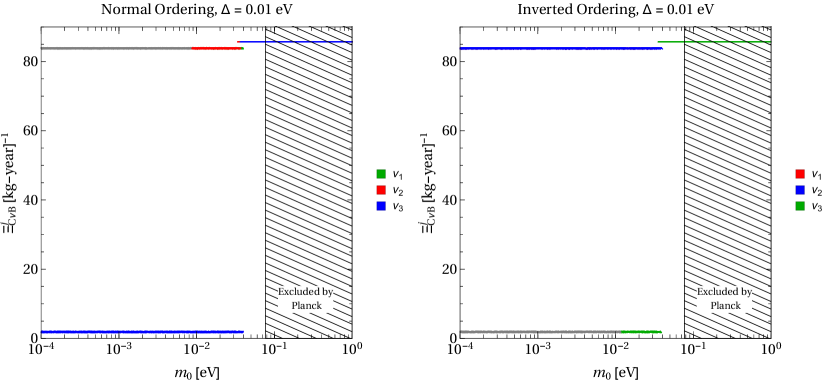
(a) $\Delta=10^{-2}$ eV

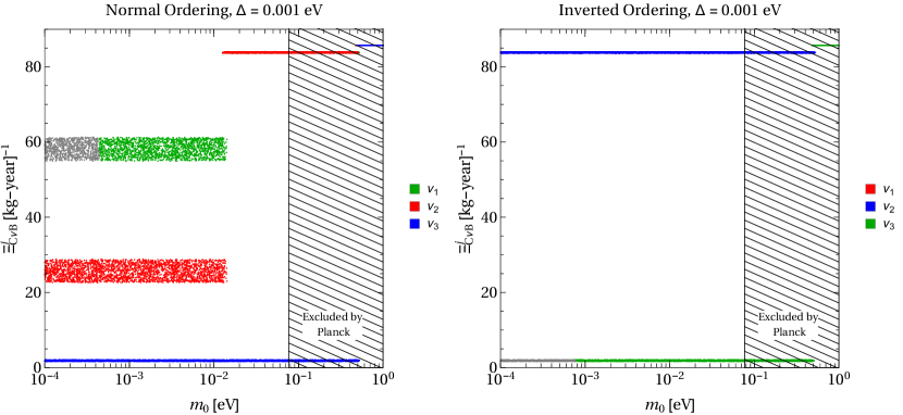
(b) $\Delta=10^{-3}$ eV

Figure 3: Dependence of the $\Xi^{j}_{\rm C\nu B}$ function of eq. (25) on the value of the lightest neutrino mass $m_{0}$. The experimental resolution is chosen to be $\Delta=0.01$ eV (upper panels) and $\Delta=0.001$ eV (lower panels), and we show both normal ordering (left panels) and inverted ordering (right panels). The three neutrino mass eigenstate contributions are shown in green ($\nu_{1}$), red ($\nu_{2}$) and blue ($\nu_{3}$). The gray points correspond to the regions that cannot be distinguished from the $\beta$-decay background. The shaded region is excluded by the Planck limit on the sum of neutrino masses Ade:2015xua .

The function $\Xi^{j}_{\rm C\nu B}$ of eq. (25) has been constructed as follows: when the mass eigenstates are degenerate, the Bhattacharya distance vanishes and $\Xi^{j}_{\rm C\nu B}$ gives the total neutrino capture rate. Since $\Xi^{j}_{\rm C\nu B}$ takes a unique value for the three neutrino states, we have that only one peak will be seen experimentally. Meanwhile, if any eigenstate is separated enough to give a distance equal or larger than $6\sigma$, the $\Xi^{j}_{\rm C\nu B}$ will correspond to the value of the capture rate for such mass eigenstate. Whether a PTOLEMY-like experiment will be able to distinguish between two or more neutrino capture peaks depends instead on the mass ordering and on the experimental resolution $\Delta$. With the expected PTOLEMY resolution of $\Delta=0.15$ eV, the Gaussian peaks for each electron will be too large to allow a distinction between the different contribution, so that a unique peak is expected. Nevertheless, we will try to understand how the electron peaks would look like for better experimental resolutions, which we take to be $\Delta=0.01$ eV and $\Delta=0.001$ eV.

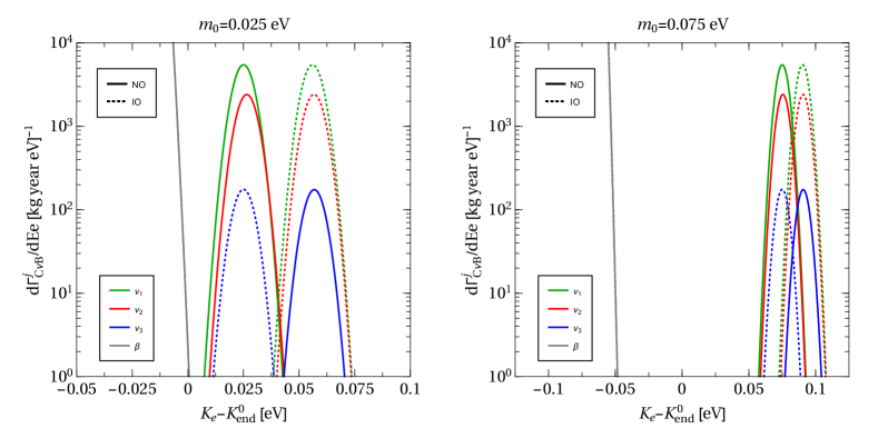
(a) $\Delta=10^{-2}$ eV

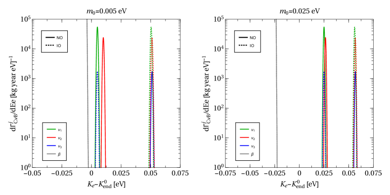
(b) $\Delta=10^{-3}$ eV

Figure 4: Simulated spectra of the electrons created by the relic neutrino capture for $\Delta=0.01$ eV (upper panels) and $\Delta=0.001$ eV (lower panels) for each mass eigenstate contribution: $\nu_{1}$ (green), $\nu_{2}$ (red), $\nu_{3}$ (blue). A few values of the lowest neutrino mass $m_{0}$ are considered to illustrate the behavior for the normal ordering (NO) and inverted ordering (IO). The gray line corresponds to the endpoint of the $\beta$-decay background.

We show in figure 3 how the $\Xi^{j}_{\rm C\nu B}$ function depend on the lightest neutrino mass $m_{0}$, for the mass eigenstates $\nu_{1}$ (green), $\nu_{2}$ (red) and $\nu_{3}$ (blue). We consider both types of mass orderings and the two resolution already mentioned, $\Delta=0.01$ eV and $\Delta=0.001$ eV. We also scan over all the neutrino parameters at $3\sigma$ Esteban:2016qun . The gray points are those that can not be distinguished from the $\beta$-decay background. The upper left panel ($\Delta=0.01$ eV, normal ordering) should be interpreted as follows: for $m_{0}\gtrsim 3\times 10^{-2}$ eV, the $\Xi^{j}_{\rm C\nu B}$ function takes only one value, so that only one peak would be measured, which corresponds to the capture of the three neutrinos. Since the peak is not gray, it can be distinguished from the $\beta$-decay background. For $8\times 10^{-3}$ eV $\lesssim m_{0}\lesssim 3\times 10^{-2}$ eV, two peaks could be measured, one due to the $\nu_{3}$ capture (blue) and the other due to $\nu_{1}$ and $\nu_{2}$ (red/green). Finally, for $m_{0}\lesssim 8\times 10^{-3}$ eV, only the $\nu_{3}$ peak can be resolved, while the $\nu_{1}+\nu_{2}$ peak cannot be discriminated from the $\beta$-decay background. The other panels can be interpreted along the same reasoning. It is interesting to notice that there is only one situation in which the three peaks can be resolved, corresponding to the normal ordering for the extreme case $\Delta=0.001$ eV. With the same resolution but inverted ordering, at most two peaks can be discriminated, since $\nu_{1}$ and $\nu_{2}$ tend to become degenerate as $m_{3}\to 0$.

To better illustrate the interplay between the experimental resolution $\Delta$ and the importance of the neutrino mass ordering, we show in figure 4 the expected spectra in a PTOLEMY-like experiment. In each plot we show normal (continuous line) and inverted (dashed line) ordering, for the two experimental resolutions we are discussing (a very agreessive $\Delta=0.01$ eV, upper panels, and an ultimate $\Delta=0.001$ eV, lower panels) and for some choices for the lightest neutrino mass. The gray line represents the $\beta$-decay background. This shows another potential problem in the peak detection; since

$$\Gamma_{\rm C\nu B}^{j}\propto\left|U_{ej}\right|^{2},$$

and

$$\left|U_{ej}\right|^{2}\simeq\left\{0.68,0.3,0.02\right\},$$

the peak due to $\nu_{3}$, although in principle distinguishable from the other peak(s), is much smaller, and will most probably be unresolved or unobservable in a real experiment.

References

- (1) S. Weinberg, Universal Neutrino Degeneracy, Phys. Rev. 128 (1962) 1457–1473.
- (2) S. Betts et al., Development of a Relic Neutrino Detection Experiment at PTOLEMY: Princeton Tritium Observatory for Light, Early-Universe, Massive-Neutrino Yield, in Proceedings, 2013 Community Summer Study on the Future of U.S. Particle Physics: Snowmass on the Mississippi (CSS2013): Minneapolis, MN, USA, July 29-August 6, 2013, 2013. arXiv:1307.4738.
- (3) A. J. Long, C. Lunardini, and E. Sabancilar, Detecting non-relativistic cosmic neutrinos by capture on tritium: phenomenology and physics potential, JCAP 1408 (2014) 038, [arXiv:1405.7654].
- (4) J. Zhang and S. Zhou, Relic Right-handed Dirac Neutrinos and Implications for Detection of Cosmic Neutrino Background, Nucl. Phys. B903 (2016) 211–225, [arXiv:1509.02274].
- (5) M.-C. Chen, M. Ratz, and A. Trautner, Nonthermal cosmic neutrino background, Phys. Rev. D92 (2015), no. 12 123006, [arXiv:1509.00481].
- (6) P. F. de Salas, S. Gariazzo, J. Lesgourgues, and S. Pastor, Calculation of the local density of relic neutrinos, arXiv:1706.09850.
- (7) B. Grzadkowski, M. Iskrzynski, M. Misiak, and J. Rosiek, Dimension-Six Terms in the Standard Model Lagrangian, JHEP 10 (2010) 085, [arXiv:1008.4884].
- (8) V. Cirigliano, M. Gonzalez-Alonso, and M. L. Graesser, Non-standard Charged Current Interactions: beta decays versus the LHC, JHEP 02 (2013) 046, [arXiv:1210.4553].
- (9) V. Cirigliano, S. Gardner, and B. Holstein, Beta Decays and Non-Standard Interactions in the LHC Era, Prog. Part. Nucl. Phys. 71 (2013) 93–118, [arXiv:1303.6953].
- (10) P. O. Ludl and W. Rodejohann, Direct Neutrino Mass Experiments and Exotic Charged Current Interactions, JHEP 06 (2016) 040, [arXiv:1603.08690].
- (11) Yu. A. Akulov and B. A. Mamyrin, Determination of the ratio of the axial-vector to the vector coupling constant for weak interaction in triton beta decay, Phys. Atom. Nucl. 65 (2002) 1795–1797. [Yad. Fiz.65,1843(2002)].
- (12) M. González-Alonso and J. Martin Camalich, Isospin breaking in the nucleon mass and the sensitivity of decays to new physics, Phys. Rev. Lett. 112 (2014), no. 4 042501, [arXiv:1309.4434].
- (13) T. Bhattacharya, V. Cirigliano, R. Gupta, H.-W. Lin, and B. Yoon, Neutron Electric Dipole Moment and Tensor Charges from Lattice QCD, Phys. Rev. Lett. 115 (2015), no. 21 212002, [arXiv:1506.04196].
- (14) S. S. Gershtein and Ya. B. Zeldovich, Meson corrections in the theory of beta decay, Zh. Eksp. Teor. Fiz. 29 (1955) 698–699.
- (15) R. P. Feynman and M. Gell-Mann, Theory of Fermi interaction, Phys. Rev. 109 (1958) 193–198.
- (16) J. C. Hardy and I. S. Towner, Superallowed nuclear beta decays: A New survey with precision tests of the conserved vector current hypothesis and the standard model, Phys. Rev. C79 (2009) 055502, [arXiv:0812.1202].
- (17) V. Mateu and J. Portoles, Form-factors in radiative pion decay, Eur. Phys. J. C52 (2007) 325–338, [arXiv:0706.1039].
- (18) T. Bhattacharya, V. Cirigliano, S. D. Cohen, A. Filipuzzi, M. Gonzalez-Alonso, M. L. Graesser, R. Gupta, and H.-W. Lin, Probing Novel Scalar and Tensor Interactions from (Ultra)Cold Neutrons to the LHC, Phys. Rev. D85 (2012) 054512, [arXiv:1110.6448].
- (19) N. Severijns, M. Beck, and O. Naviliat-Cuncic, Tests of the standard electroweak model in beta decay, Rev. Mod. Phys. 78 (2006) 991–1040, [nucl-ex/0605029].
- (20) O. Naviliat-Cuncic and M. González-Alonso, Prospects for precision measurements in nuclear decay at the LHC era, Annalen Phys. 525 (2013) 600–619, [arXiv:1304.1759].
- (21) B. A. Campbell and D. W. Maybury, Constraints on scalar couplings from , Nucl. Phys. B709 (2005) 419–439, [hep-ph/0303046].
- (22) G. Duda, G. Gelmini, and S. Nussinov, Expected signals in relic neutrino detectors, Phys. Rev. D64 (2001) 122001, [hep-ph/0107027].
- (23) L. A. Anchordoqui, H. Goldberg, and G. Steigman, Right-Handed Neutrinos as the Dark Radiation: Status and Forecasts for the LHC, Phys. Lett. B718 (2013) 1162–1165, [arXiv:1211.0186].
- (24) A. Solaguren-Beascoa and M. C. Gonzalez-Garcia, Dark Radiation Confronting LHC in Z’ Models, Phys. Lett. B719 (2013) 121–125, [arXiv:1210.6350].
- (25) Planck Collaboration, P. A. R. Ade et al., Planck 2015 results. XIII. Cosmological parameters, Astron. Astrophys. 594 (2016) A13, [arXiv:1502.01589].
- (26) M. Blennow, Prospects for cosmic neutrino detection in tritium experiments in the case of hierarchical neutrino masses, Phys. Rev. D77 (2008) 113014, [arXiv:0803.3762].
- (27) Y. F. Li, Z.-z. Xing, and S. Luo, Direct Detection of the Cosmic Neutrino Background Including Light Sterile Neutrinos, Phys. Lett. B692 (2010) 261–267, [arXiv:1007.0914].
- (28) A. Bhattacharyya, On a measure of divergence between two statistical populations defined by their probability distributions, Bull. Calcutta Math. Soc. 35 (1943) 99–109.
- (29) I. Esteban, M. C. Gonzalez-Garcia, M. Maltoni, I. Martinez-Soler, and T. Schwetz, Updated fit to three neutrino mixing: exploring the accelerator-reactor complementarity, JHEP 01 (2017) 087, [arXiv:1611.01514].