On Birkhoff’s theorem in ghost-free bimetric theory

Abstract

We consider the Hassan-Rosen bimetric field equations in vacuum when the two metrics share a single common null direction in a spherically symmetric configuration. By solving these equations, we obtain a class of exact solutions of the generalized Vaidya type parametrized by an arbitrary function. Besides not being asymptotically flat, the found solutions are nonstationary admitting only three global spacelike Killing vector fields which are the generators of spatial rotations. Hence, these are spherically symmetric bimetric vacuum solutions with the minimal number of isometries. The absence of staticity formally disproves an analogue statement to Birkhoff’s theorem in the ghost-free bimetric theory which would state that a spherically symmetric solution is necessarily static in empty space.

1 Introduction and summary

The framework of this paper is the Hassan-Rosen (HR) ghost-free bimetric theory Hassan:2011zd , which is a classical nonlinear theory of two interacting spin-2 fields. As shown in Hassan:2011zd ; Hassan:2011ea , the HR bimetric theory is free of instabilities such as the Boulware-Deser ghost Boulware:1973my . An unambiguous definition of the theory which guaranties the existence of a spacetime interpretation is given in Hassan:2017ugh . The HR theory is closely related to de Rham-Gabadadze-Tolley (dRGT) massive gravity deRham:2010ik ; deRham:2010kj , which is a nonlinear theory of a massive spin-2 field, proven to be ghost-free in Hassan:2011hr . For recent reviews of these theories, see Schmidt-May:2015vnx ; deRham:2014zqa .

Although understanding of the HR theory has seen a considerable development in recent years, not many exact vacuum solutions have been found. This is not surprising as the bimetric field equations are more than doubled in number when compared to General relativity (GR). Consequently, the majority of known exact vacuum solutions have both metrics in standard GR form (see Schmidt-May:2015vnx and references therein, and also more recently Sushkov:2015fma ; Nersisyan:2015oha ; Mazuet:2015pea ; Babichev:2015xha ; Enander:2015kda ; Li:2016fbf ; Hu:2016hpm ; Li:2016tcn ; Torsello:2017cmz ), where the only nonstationary and spherically symmetric vacuum solution was found in Hassan:2012gz . The other issue is an analogue statement to Birkhoff’s theorem Birkhoff:1923 ; Eiesland:1925 ; Schleich:2009uj which would claim that spherically symmetric bimetric solutions in empty space are necessarily static. It is argued that such a statement is absent in the bimetric theory Babichev:2015xha .

The main result of this paper is a class of exact bimetric vacuum solutions which are nonstationary where the null tetrads Stephani:2009exact of the two metrics have a single common null direction in a spherically symmetric configuration. Contrary to GR, where spherically symmetric vacuum solutions admit at least four isometries, the found solutions have only three Killing vector fields that are the generators of spatial rotations. Moreover, the solutions are conformally flat. The metrics are of the generalized Vaidya type parametrized by an arbitrary function, here denoted the curvature field. For a constant curvature field, one gets a proportional and maximally symmetric GR solution. The nonstationarity of this and the solution from Hassan:2012gz formally contradicts an analogue statement to Birkhoff’s theorem for the ghost-free bimetric theory. Before summarizing results in more detail, we overview the ghost-free bimetric theory and its field equations in the absence of matter.

1.1 Ghost-free bimetric action and equations of motion

In vacuum, the Hassan-Rosen action comprises two Einstein-Hilbert terms with Planck masses $M_{g}$ and $M_{f}$ coupled through the ghost-free interaction term Hassan:2011zd ,

$$S_{\mathrm{HR}} =\frac{1}{2}M_{g}^{2}\!\int\mathrm{d}^{4}x\sqrt{-g}\,R_{g}+\frac{1}{2}M_{f}^{2}\!\int\mathrm{d}^{4}x\sqrt{-f}\,R_{f}-m^{4}\!\int\mathrm{d}^{4}x\sqrt{-g}\,V(S).$$ (1)

The absence of ghosts is ensured by the potential $V(S)$ of the following form,

$$V(S)\coloneqq\sum_{n=0}^{4}\beta_{n}\,e_{n}(S),$$ (2)

where $S$ denotes the square root of the operator $g^{\mu\rho}f_{\rho\nu}$. In matrix notation, $S$ is the square root matrix function $S=\sqrt{g^{-1}f}$. The potential is parametrized by real constants, $\beta_{n}$, $n=0,...,4$, which are free parameters of the theory. The coefficients $e_{n}(S)$ in (2) are the elementary symmetric polynomials, which are the scalar invariants of $S$ obtained through the generating function macdonald:1998a ,

$$E(t,S)=\det(I+tS)=\sum_{n=0}^{\infty}e_{n}(S)\,t^{n}.$$ (3)

Note that $e_{n}(S)=0$ for $n>4$ due to the Cayley-Hamilton theorem.

By varying (1) with respect to $g$ and $f$, we obtain the equations of motion Hassan:2014vja ,

$$G_{g}{}^{\mu}{}_{\nu}+\frac{m^{4}}{M_{g}^{2}}V_{g}{}^{\mu}{}_{\nu}(S)=0,\qquad G_{f}{}^{\mu}{}_{\nu}+\frac{m^{4}}{M_{f}^{2}}V_{f}{}^{\mu}{}_{\nu}(S)=0.$$ (4a)

Here, $G_{g}$ and $G_{f}$ are the Einstein tensors of $g$ and $f$, respectively, given in operator form, while $V_{g}$ and $V_{f}$ are contributions of the potential (2),

$$V_{g}(S) =\sum_{n=0}^{3}\beta_{n}\sum_{k=0}^{n}(-1)^{n+k}e_{k}(S)\,S^{n-k},$$ (5a)

$$V_{f}(S) =\sum_{n=0}^{3}\beta_{4-n}\sum_{k=0}^{n}(-1)^{n+k}e_{k}(S^{-1})\,S^{-n+k},$$ (5b)

which are coupled through the algebraic identity Hassan:2014vja ,

$$V_{g}(S)+\det(S)\,V_{f}(S)=V(S).$$ (6)

Finally, the equations of motion (4) are supplemented by two Bianchi constraints,

$$\nabla_{\mu}\left[V_{g}{}^{\mu}{}_{\nu}(S)\right]=0,\qquad\tilde{\nabla}_{\mu}\left[V_{f}{}^{\mu}{}_{\nu}(S)\right]=0,$$ (7)

where $\nabla_{\mu}$ and $\tilde{\nabla}_{\mu}$ are the covariant derivatives compatible with $g$ and $f$, respectively. However, assuming a nonsingular $S$, the two Bianchi constraints are not independent since the invariance of the interaction term under the diagonal diffeomorphism group implies the identity Damour:2002ws ,

$$\nabla_{\mu}\left[V_{g}{}^{\mu}{}_{\nu}(S)\right]+\det(S)\,\tilde{\nabla}_{\mu}\left[V_{f}{}^{\mu}{}_{\nu}(S)\right]=0.$$ (8)

1.2 Summary of results

We consider bimetric field equations in vacuum when the null tetrads of the two metrics share a single common null direction throughout the spacetime in a spherically symmetric configuration. Locally, this configuration is not simultaneously diagonalizable and referred to as Type IIa by the algebraic classification of square roots in Hassan:2017ugh . By solving the equations in the spherically symmetric chart $(v,r,\theta,\phi)$, we obtain the class of solutions parametrized by an arbitrary function $\lambda(v)>0$,

$$g =-\left(1-\frac{1}{3}\Lambda(v)\,r^{2}\right)\mathrm{d}v^{2}+2\,\mathrm{d}v\,\mathrm{d}r+r^{2}\left(\mathrm{d}\theta^{2}+\sin^{2}\theta\,\mathrm{d}\phi^{2}\right)\!,$$ (9a)

$$f =-\lambda^{2}(v)\left[\left(1-\frac{1}{3}\Lambda(v)\,r^{2}-2\frac{\lambda^{\prime}(v)}{\lambda(v)}\,r\right)\mathrm{d}v^{2}+2\,\mathrm{d}v\,\mathrm{d}r+r^{2}\left(\mathrm{d}\theta^{2}+\sin^{2}\theta\,\mathrm{d}\phi^{2}\right)\right]\!,$$ (9b)

where,

$$\Lambda(v)\coloneqq 3\beta_{2}m^{4}\left(M_{f}^{-2}+M_{g}^{-2}\lambda^{2}(v)\right)\!.$$ (10)

The field $\Lambda(v)$ completely defines the class of solutions (9) through the parameters $\Lambda_{0}\coloneqq 3\beta_{2}m^{4}M_{g}^{-2}$, $\alpha\coloneqq M_{f}/M_{g}$, and the form of $\lambda(v)$. The function $\lambda(v)$ is undetermined by equations of motion, provided that the values of the rest of the $\beta$-parameters satisfy,

$$\beta_{0}=3\beta_{2}\alpha^{-2},\qquad\beta_{4}=3\beta_{2}\alpha^{2},\qquad\beta_{1}=\beta_{3}=0.$$ (11)

These values are known as the partially massless (PM) parameters since they provide a de Sitter background in the context of PM bimetric gravity Hassan:2012gz . For arbitrary $\beta$-parameters, the equation of motion sets a constant $\lambda(v)$ with a value given by the parameters. In the following, the class of solutions (9)–(11) will also be referred to simply as “the solution”.

The Weyl tensor vanishes identically in both sectors, so the solution is conformally flat (Petrov Type O). As can be shown, the field $\Lambda(v)$ enters all curvature scalars; hence, the solution exhibits a variable curvature parametrized by $\Lambda(v)$ which is accordingly called the curvature field. For a constant $\Lambda(v)$, the solution becomes proportional and maximally symmetric (i.e., an ordinary GR solution: Minkowski, de Sitter or anti-de Sitter). The solution (9) is not asymptotically flat, unless $\Lambda(v)=0$.

Physically, the effective stress-energy tensors (5) of the solution are nonperfect null fluids of Type II in GR Hawking:1973large and the metrics can be classified as being of the generalized Vaidya type. In GR, an ordinary Vaidya metric is a solution of the Einstein field equations describing the spacetime of a spherically symmetric inhomogeneous imploding (exploding) null dust fluid Vaidya:1951zza . However, the metrics (9) have no curvature singularities. They have the form of the Husain null fluid spacetimes Husain:1995bf and the generalized Vaidya metric Wang:1998qx analyzed in Ibohal:2004kk ; Ibohal:2006ez ; Ibohal:2009px in the context of nonstationary de Sitter cosmological models in GR.

For a variable $\Lambda(v)$, the solution is nonstationary admitting only three global spacelike Killing vector fields that are the generators of spatial rotations. In GR, spherically symmetric vacuum solutions have from ten (corresponding to de Sitter, Minkowski, and anti-de Sitter metrics) to four Killing vector fields (the minimal symmetry) Bokhari:1990a6 . Thus, contrary to GR, the found class of solutions comprises only three Killing vector fields. Importantly, the absence of staticity contradicts an analogue statement to Birkhoff’s theorem in the ghost-free bimetric theory. Nonetheless, the solution admits conformal Killing vector fields (see subsection 2.4 for more details).

The nonstationarity (and thus nonstaticity) of the solution is best illustrated by plotting the radial null geodesics of $g$ and $f$ in a local patch $(v,r,\theta,\phi)$. This is done in Figure 1 for (a) the nonstationary case with $\lambda(v)\propto\exp(v)$, and (b) the static case with $\lambda(v)=\mathrm{const}$. The broken translational symmetry and the nonhomogeneity is clearly visible from Figure 1(a). Also, the case (a) looks almost static when $\lambda^{\prime}(v)\to 0$ in the limit $v\to-\infty$.

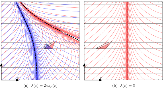
Figure 1: Null radial geodesics for (a) $\lambda(v)=2\exp(v)$ and (b) $\lambda(v)=3$ for $\alpha=1$, $\beta_{2}=1/3$ with sample future-pointing null cones. Ingoing null radial geodesics (common to $g$ and $f$) are horizontal and depicted in black, outgoing geodesics of $g$ are in red and outgoing geodesics of $f$ are in blue. Dashed lines are the cosmological horizons. The geodesics of $g$ and $f$ coincide in the right panel since the solution is proportional. Note the broken translational symmetry in the left panel.

The rest of this paper is organized as follows. The spacetime ansatz and the equations of motion are stated in subsection 2.1. The equations of motion are solved in subsection 2.2. The properties of the found solution are given in subsection 2.3. The Killing and conformal Killing equations are solved in subsection 2.4. A physical interpretation of the solution is given in subsection 2.5. The paper ends with a short discussion in section 3. The relevant chart transition maps are given in the appendix.

2 Bimetric vacuum solutions of the generalized Vaidya type

2.1 The configuration with one common null direction

In this subsection, we write the ansatz for the spherically symmetric bimetric spacetime where the two metrics share one common null direction, denoted Type IIa in Hassan:2017ugh .

A spherically symmetric metric is one which remains invariant under rotations. In particular, the isometry group of a spherically symmetric metric contains a subgroup isomorphic to SO(3). The orbits of this subgroup are two-dimensional spheres. In a spherical chart $(\theta,\phi)$, the metric on each orbit two-sphere is induced by the spacetime metric and takes the form $r^{2}\left(\mathrm{d}\theta^{2}+\sin^{2}\theta\,\mathrm{d}\phi^{2}\right)$ where the scalar field $r^{2}$ parametrizes the area of the two-sphere Wald:1984 . Completing the spherical chart with two additional spacetime coordinates $a$ and $b$, the most general spherically symmetric metric in a chart $(a,b,\theta,\phi)$ can be written,

$$-A(a,b)\,\mathrm{d}a^{2}+B(a,b)\,\mathrm{d}b^{2}+2C(a,b)\,\mathrm{d}a\,\mathrm{d}b+r(a,b)^{2}\mathrm{d}\Omega^{2},$$ (12)

where $\mathrm{d}\Omega^{2}\coloneqq\mathrm{d}\theta^{2}+\sin^{2}\theta\,\mathrm{d}\phi^{2}$. For two spherically symmetric metrics, we have two sets of fields $A$, $B$, $C$ and $r$. The gauge freedom allows a reparametrization of one of the coordinates, for example, setting $b=r$ along the radial coordinate of one of the metrics. Since one of the metrics can always be diagonalized, the bimetric spherically symmetric setup has six independent scalar fields.

The second assumption is that the two metrics have a common null direction throughout the spacetime. Suggestively choosing $a=v$, the ansatz in the chart $(v,r,\theta,\phi)$ reads,

$$g =-\mathrm{e}^{2p(v,r)}G(v,r)\,\mathrm{d}v^{2}+2\mathrm{e}^{p(v,r)}\mathrm{d}v\,\mathrm{d}r+r^{2}\mathrm{d}\Omega^{2},$$ (13a)

$$f =\lambda^{2}(v,r)\,\left[-\mathrm{e}^{2q(v,r)}F(v,r)\,\mathrm{d}v^{2}+2\mathrm{e}^{q(v,r)}\mathrm{d}v\,\mathrm{d}r+r^{2}\mathrm{d}\Omega^{2}\right]\!,$$ (13b)

where $G$, $F$, $p$, $q$ and $\lambda$ are scalar fields. Relative to both metrics, $v=\mathrm{const}$ are spherically symmetric null surfaces. Compared to the most general ansatz, the absence of the $\mathrm{d}r^{2}$-component for $f$ is imposed by the common null direction requirement. Further setting $p\equiv 0$ and $q\equiv 0$ makes the contributions of the potential (5) of Type II in Hawking:1973large ; Martin-Moruno:2017exc (see also subsection 2.5). As a consequence, the degrees of freedom in this setup are contained in the metric fields $G(v,r)$, $F(v,r)$ and $\lambda(v,r)$. At this point, there is no particular attribute attached to the null coordinate $v$. After solving the equations, the coordinate $v$ will be interpreted as the advanced (ingoing) time. Substituting $v$ by $-u$, we can repeat our analysis and consider the chart in terms of the retarded (outgoing) time $u$.

The complex null tetrads Stephani:2009exact of $g$ and $f$ are given by the vector fields,

$$\ell_{g} =-\partial_{r}, \quad\qquad\ell_{f} =-\lambda(v,r)\,\partial_{r},$$ (14a)

$$n_{g} =\partial_{v}+\frac{1}{2}G(v,r)\,\partial_{r}, n_{f} =\lambda(v,r)\left(\partial_{v}+\frac{1}{2}F(v,r)\,\partial_{r}\right)\!,$$ (14b)

$$m_{g} =\frac{1}{\sqrt{2}r}\left(\partial_{\theta}+\mathrm{i}\csc\theta\,\partial_{\phi}\right), m_{f} =\frac{1}{\sqrt{2}r}\lambda(v,r)\left(\partial_{\theta}+\mathrm{i}\csc\theta\,\partial_{\phi}\right),$$ (14c)

satisfying respective $\ell^{a}n_{a}=-1$, $m^{a}\bar{m}_{a}=1$ with all other contractions vanishing. Then, in component form, the two metric inverses read,

$$g^{\mu\nu}=-2\ell_{g}^{(\mu}n_{g}^{\nu)}+2m_{g}^{(\mu}\bar{m}_{g}^{\nu)},\,\qquad f^{\mu\nu}=-2\ell_{f}^{(\mu}n_{f}^{\nu)}+2m_{f}^{(\mu}\bar{m}_{f}^{\nu)}.\qquad\ \$$ (15)

Clearly, the null radial directions $\ell_{g}$ and $\ell_{f}$ are proportional for the two metrics while the null radial directions $n_{g}$ and $n_{f}$ become proportional for $F(v,r)=G(v,r)$. Also, $m_{g}$ and $m_{f}$ are proportional as a result of spherical symmetry.

In matrix notation, the ansatz can be written,

$$g =\left(\begin{array}[]{cc|cc}-G(v,r)&1\hfil\lx@intercol\color[rgb]{.75,.75,.75}\pgfsys@color@gray@fill{.75&0&0\\ 1&0\hfil\lx@intercol\color[rgb]{.75,.75,.75}\pgfsys@color@gray@fill{.75&0&0\\ \hline\cr 0&0\hfil\lx@intercol\color[rgb]{.75,.75,.75}\pgfsys@color@gray@fill{.75&r^{2}&0\\ 0&0\hfil\lx@intercol\color[rgb]{.75,.75,.75}\pgfsys@color@gray@fill{.75&0&r^{2}\sin^{2}\theta\end{array}\right)\!,}}}}$$ (16e)

$$f =\left(\begin{array}[]{cc|cc}-\lambda^{2}(v,r)F(v,r)&\lambda^{2}(v,r)\hfil\lx@intercol\color[rgb]{.75,.75,.75}\pgfsys@color@gray@fill{.75&0&0\\ \lambda^{2}(v,r)&0\hfil\lx@intercol\color[rgb]{.75,.75,.75}\pgfsys@color@gray@fill{.75&0&0\\ \hline\cr 0&0\hfil\lx@intercol\color[rgb]{.75,.75,.75}\pgfsys@color@gray@fill{.75&\lambda^{2}(v,r)r^{2}&0\\ 0&0\hfil\lx@intercol\color[rgb]{.75,.75,.75}\pgfsys@color@gray@fill{.75&0&\lambda^{2}(v,r)r^{2}\sin^{2}\theta\end{array}\right)\!.}}}}$$ (16j)

For $\lambda(v,r)>0$, the principal square root $S=\sqrt{g^{-1}f}$ reads,

$$S=\left(\begin{array}[]{cc|cc}\lambda(v,r)&0\hfil\lx@intercol\color[rgb]{.75,.75,.75}\pgfsys@color@gray@fill{.75&0&0\\ \frac{1}{2}\lambda(v,r)\left(G(v,r)-F(v,r)\right)&\lambda(v,r)\hfil\lx@intercol\color[rgb]{.75,.75,.75}\pgfsys@color@gray@fill{.75&0&0\\ \hline\cr 0&0\hfil\lx@intercol\color[rgb]{.75,.75,.75}\pgfsys@color@gray@fill{.75&\lambda(v,r)&0\\ 0&0\hfil\lx@intercol\color[rgb]{.75,.75,.75}\pgfsys@color@gray@fill{.75&0&\lambda(v,r)\end{array}\right)\!.}}}}$$ (17)

In general, $S$ can have the Segre types $[1111]$, $[211]$, $[z\bar{z}11]$ and $[31]$. For $G(v,r)\neq F(v,r)$, the square root (17) has Segre characteristics $[(211)]$, which is referred to as Type IIa by the algebraic classification of bimetric solutions in Hassan:2017ugh . The contributions of the potential (5) are matrix-valued functions of the square root (17) and have the same Segre type. Note that the stress-energy tensors of types $[31]$ and $[z\bar{z}11]$ are known to violate the weak energy condition in GR (see Theorem 7.11 in Hall:2004symmetries and also Hall:1983a ; Hawking:1973large ). Hence, by GR standards, only types $[1111]$ and $[211]$ potentially bear physical viability.

2.2 The equations of motion

Here we present and solve the equations of motion for the ansatz (16). For convenience, we introduce the Planck mass ratio $\alpha\coloneqq M_{f}/M_{g}$ and also absorb $m^{4}M_{g}^{-2}$ in the $\beta$-parameters, $m^{4}M_{g}^{-2}\beta_{n}\to\beta_{n}$. We can always recover the mass terms by the reverse procedure at any point. Note that the $\beta$-parameters are not any more dimensionless after this substitution. The bimetric field equations (4) and the Bianchi constraint (7) become,

$$0 =?{\mbox{$G_{g}$}}^{\mu}{}_{\nu}?+?{\mbox{$V_{g}(S)$}}^{\mu}{}_{\nu}?,$$ (18)

$$0 =?{\mbox{$G_{f}$}}^{\mu}{}_{\nu}?+\alpha^{-2}?{\mbox{$V_{f}(S)$}}^{\mu}{}_{\nu}?,$$ (19)

$$0 =\nabla_{\mu}\left[?{\mbox{$V_{g}(S)$}}^{\mu}{}_{\nu}?\right].$$ (20)

To further simplify equations, following Kocic:2017wwf , we introduce the symmetric function $\left\langle\cdot\right\rangle_{k}^{n}$ for a set of variables $x_{1},\dots,x_{d}$ or a single repeated variable $\lambda$, defined by,

$$\left\langle x_{1},\dots,x_{d}\right\rangle_{k}^{n}\coloneqq\sum_{i=0}^{n}\beta_{i+k}\,e_{i}(x_{1},\dots,x_{d}),\qquad\left\langle\lambda\right\rangle_{k}^{n}\coloneqq\sum_{i=0}^{n}\binom{n}{i}\beta_{i+k}\lambda^{i}.$$ (21)

If the argument of $\left\langle\cdot\right\rangle_{k}^{n}$ is a matrix, its eigenvalues are used; for example, we can express the potential as $V(S)=\left\langle S\right\rangle_{0}^{4}$.

Substituting (13) in (18)-(20) gives the following system of equations,

$$0 =r^{2}\left\langle\lambda\right\rangle_{0}^{3}+G-1+r\partial_{r}G,$$ (18a)

$$0 =r\lambda\left\langle\lambda\right\rangle_{1}^{2}(F-G)-2\partial_{v}G,$$ (18b)

$$0 =2r\left\langle\lambda\right\rangle_{0}^{3}+r\partial_{r}^{2}G+2\partial_{r}G,$$ (18c)

$$0 =\alpha^{-2}r^{2}\lambda\left\langle\lambda\right\rangle_{1}^{3}+\lambda^{2}\left(F-1+r\partial_{r}F\right)+4r\lambda\left(F\partial_{r}\lambda+\partial_{v}\lambda\right)$$

$$\qquad+\,r^{2}\partial_{r}\lambda\left(-F\partial_{r}\lambda+2\partial_{v}\lambda\right)+\lambda r^{2}\partial_{r}F\partial_{r}\lambda+2\lambda r^{2}\left(F\partial_{r}^{2}\lambda+\partial_{v}\partial_{r}\lambda\right),$$ (19a)

$$0 =2\left(\partial_{r}\lambda\right)^{2}-\lambda\partial_{r}^{2}\lambda,$$ (19b)

$$0 =\alpha^{-2}r\lambda\left(F-G\right)\left\langle\lambda\right\rangle_{1}^{2}+2\lambda^{2}\partial_{v}F-8r\partial_{v}\lambda\left(F\partial_{r}\lambda+\partial_{v}\lambda\right)$$

$$\qquad+\,2r\lambda\left(\partial_{v}F\partial_{r}\lambda-\partial_{r}F\partial_{v}\lambda+2F\partial_{v}\partial_{r}\lambda+2\partial_{v}^{2}\lambda\right),$$ (19c)

$$0 =\alpha^{-2}r^{2}\lambda\left\langle\lambda\right\rangle_{1}^{3}+\lambda^{2}\left(F-1+r\partial_{r}F\right)+4r\lambda\left(F\partial_{r}\lambda+\partial_{v}\lambda\right)$$

$$\qquad+\,r^{2}\partial_{r}\lambda\left(3F\partial_{r}\lambda+2\partial_{v}\lambda\right)+r^{2}\lambda\left(\partial_{r}F\partial_{r}\lambda+2\partial_{v}\partial_{r}\lambda\right),$$ (19d)

$$0 =2\alpha^{-2}r\lambda\left\langle\lambda\right\rangle_{1}^{3}+\lambda^{2}\left(2\partial_{r}F+r\partial_{r}^{2}F\right)+4\lambda\left(F\partial_{r}\lambda+\partial_{v}\lambda\right)$$

$$\qquad-\,2r\partial_{r}\lambda\left(F\partial_{r}\lambda+2\partial_{v}\lambda\right)+4r\lambda\left(\partial_{r}F\partial_{r}\lambda+F\partial_{r}^{2}\lambda+2\partial_{v}\partial_{r}\lambda\right),$$ (19e)

$$0 =2r(F-G)\left\langle\lambda\right\rangle_{1}^{1}\partial_{r}\lambda-r\lambda\left\langle\lambda\right\rangle_{1}^{2}\left(\partial_{r}F-\partial_{r}G\right)$$

$$\qquad-\,\left(F-G\right)\left\langle\lambda\right\rangle_{1}^{2}\left(2\lambda+3r\partial_{r}\lambda\right)-6r\left\langle\lambda\right\rangle_{1}^{2}\partial_{v}\lambda,$$ (20a)

$$0 =\left\langle\lambda\right\rangle_{1}^{2}\partial_{r}\lambda.$$ (20b)

Solving the system is done in several steps, summarized below.

Step 1.

Since $\partial_{r}\lambda(v,r)=0$ from the Bianchi constraint (20b), $\lambda(v,r)=\lambda(v)$.

Step 2.

From (18a) and (18c), we get $2(1-G)+r^{2}\partial_{r}^{2}G=0$. Solving this yields,

$$G(v,r)=1+a(v)\,r^{2}+\frac{b(v)}{r},$$ (22)

where $a(v)$ and $b(v)$ are arbitrary functions.

Step 3.

After substituting (22), from (18a) we can express $a(v)$ in terms of $\lambda(v)$ as,

$$a(v)=-\frac{1}{3}\left\langle\lambda(v)\right\rangle_{0}^{3}=-\frac{1}{3}\left(\beta_{0}+3\beta_{1}\lambda(v)+3\beta_{2}\lambda^{2}(v)+\beta_{3}\lambda^{3}(v)\right),$$ (23)

which we again substitute back in the equations. The simplification of the derivatives of $a(v)$ is done using the relation,

$$\partial_{v}\left\langle\lambda(v)\right\rangle_{k}^{n}=n\left\langle\lambda(v)\right\rangle_{k+1}^{n-1}\,\lambda^{\prime}(v)\quad\implies\quad a^{\prime}(v)=-\lambda^{\prime}(v)\left\langle\lambda(v)\right\rangle_{1}^{2}\,.$$ (24)

Step 4.

From (18b), we can express $F(v,r)$ in terms of $\lambda(v)$ and $b(v)$ as,

$$F(v,r) =1-\frac{1}{3}r^{2}\left\langle\lambda(v)\right\rangle_{0}^{3}+\frac{b(v)}{r}-2r\frac{\lambda^{\prime}(v)}{\lambda(v)}+2\frac{b^{\prime}(v)}{\lambda r^{2}\left\langle\lambda(v)\right\rangle_{1}^{2}}$$ (25)

$$=G(v,r)-2r\frac{\lambda^{\prime}(v)}{\lambda(v)}+2\frac{b^{\prime}(v)}{\lambda r^{2}\left\langle\lambda(v)\right\rangle_{1}^{2}}\,.$$ (26)

Step 5.

Subtracting (19a) and (19e), we obtain $b^{\prime}(v)/\left\langle\lambda(v)\right\rangle_{1}^{2}=0$; thus $b(v)=b_{0}$ where $b_{0}$ is a real constant.

Step 6.

Using $G(v,r)=1-\frac{1}{3}r^{2}\left\langle\lambda(v)\right\rangle_{0}^{3}+\frac{b_{0}}{r}$ and $F(v,r)=1-\frac{1}{3}r^{2}\left\langle\lambda(v)\right\rangle_{0}^{3}+\frac{b_{0}}{r}-2r\frac{\lambda^{\prime}(v)}{\lambda(v)}$ significantly reduces the equations to become mostly algebraical; for example, equation (19a) becomes $\alpha^{2}\lambda\left\langle\lambda\right\rangle_{0}^{3}-\left\langle\lambda\right\rangle_{1}^{3}=0$, that is,

$$\alpha^{2}\beta_{3}\lambda^{4}(v)+\left(3\alpha^{2}\beta_{2}-\beta_{4}\right)\lambda^{3}(v)+3\left(\alpha^{2}\beta_{1}-\beta_{3}\right)\lambda^{2}(v)+\left(\alpha^{2}\beta_{0}-3\beta_{2}\right)\lambda(v)-\beta_{1}=0.$$ (27)

For a given set of $\beta$-parameters, the above quartic equation fully defines $\lambda(v)=\mathrm{const}$.

Now, let us assume that $\lambda(v)$ is not constant, i.e., $\lambda^{\prime}(v)\neq 0$. Then (27) must hold for an arbitrary $\lambda(v)$. The parameter combination that keeps $\lambda(v)$ undetermined is: $\beta_{0}=3\beta_{2}\alpha^{-2}$, $\beta_{4}=3\beta_{2}\alpha^{2}$, $\beta_{1}=\beta_{3}=0$. This gives,

$$a(v)=-\frac{1}{3}\left\langle\lambda(v)\right\rangle_{0}^{3}=-\beta_{2}\left(\alpha^{-2}+\lambda^{2}(v)\right).$$ (28)

Note that $\lambda(v)$ can be chosen freely as an integration function baring no dynamics.

Step 7.

Finally, using the above $\beta$-parameters reduces (18)-(20) to a single equation $b_{0}\lambda^{\prime}(v)=0$, which requires $b_{0}$ to vanish identically in order to have an arbitrary $\lambda(v)$. Otherwise, if $\lambda(v)$ was taken to be constant in Step 6, $b_{0}$ would be arbitrary.

Collecting the results for $a(v)$ and $b(v)$ gives the final form of $F(v,r)$ and $G(v,r)$ as a solution, which is presented in the following subsection.

2.3 The solution and its geometry

In this subsection, we quote the found solution and analyze its geometrical properties.

By solving (18)-(20), we obtained the class of exact solutions,

$$G(v,r) =1-\beta_{2}\left(\alpha^{-2}+\lambda^{2}(v)\right)r^{2},$$ (29a)

$$F(v,r) =1-\beta_{2}\left(\alpha^{-2}+\lambda^{2}(v)\right)r^{2}-2\frac{\lambda^{\prime}(v)}{\lambda(v)}r,$$ (29b)

where $\lambda(v)>0$ is an arbitrary function having no dynamics. The dimensionfull $\beta_{2}$ and the dimensionless $\alpha$ are the only free parameters of the theory. Solving the equations of motion in one branch also gave,

$$\beta_{0}=3\beta_{2}\alpha^{-2},\qquad\beta_{4}=3\beta_{2}\alpha^{2},\qquad\beta_{1}=\beta_{3}=0.$$ (30)

This condition is the same as the one imposed for the de Sitter background in the context of partially massless bimetric gravity Hassan:2012gz .

Using (29), the metrics (13) become,

$$g =-\left[1-\beta_{2}\left(\alpha^{-2}+\lambda^{2}(v)\right)r^{2}\right]\mathrm{d}v^{2}+2\,\mathrm{d}v\,\mathrm{d}r+r^{2}\mathrm{d}\Omega^{2},$$ (31a)

$$f =\lambda^{2}(v)\left\{-\left[1-\beta_{2}\left(\alpha^{-2}+\lambda^{2}(v)\right)r^{2}-2r\frac{\lambda^{\prime}(v)}{\lambda(v)}\right]\mathrm{d}v^{2}+2\,\mathrm{d}v\,\mathrm{d}r+r^{2}\mathrm{d}\Omega^{2}\right\}\!.$$ (31b)

The square root (17) is accordingly,

$$S=r\lambda^{\prime}(v)\,\partial_{r}\otimes\mathrm{d}v+\lambda(v)\left[\,\partial_{v}\otimes\mathrm{d}v+\partial_{r}\otimes\mathrm{d}r+\partial_{\theta}\otimes\mathrm{d}\theta+\partial_{\phi}\otimes\mathrm{d}\phi\,\right],$$ (32)

with the only off-diagonal component $?{\mbox{$S$}}^{r}{}_{v}?=\frac{1}{2}\lambda\left(G-F\right)=r\,\lambda^{\prime}(v)$.

One of the features of the solution is a variable cosmological ‘constant’, or rather the curvature field,

$$\Lambda(v)\coloneqq 3\beta_{2}\left(\alpha^{-2}+\lambda^{2}(v)\right),$$ (33)

in terms of which we can write (31) as,

$$g =-\left(1-\frac{1}{3}\Lambda(v)\,r^{2}\right)\mathrm{d}v^{2}+2\,\mathrm{d}v\,\mathrm{d}r+r^{2}\mathrm{d}\Omega^{2},$$ (34a)

$$f =-\lambda^{2}(v)\left[\left(1-\frac{1}{3}\Lambda(v)\,r^{2}-2\frac{\lambda^{\prime}(v)}{\lambda(v)}\,r\right)\mathrm{d}v^{2}+2\,\mathrm{d}v\,\mathrm{d}r+r^{2}\mathrm{d}\Omega^{2}\right]\!.$$ (34b)

Equation (33) completely defines the class of solutions through the parameters $\beta_{2}$, $\alpha$ and the form of $\lambda(v)$. Reinstating the original dimensionless $\beta_{2}$, (33) becomes $\Lambda(v)=3\beta_{2}m^{4}\left(M_{f}^{-2}+M_{g}^{-2}\lambda^{2}(v)\right)$.

In terms of the curvature field, the bimetric potential reads $V(S)=\alpha^{2}\Lambda^{2}(v)/(3\beta_{2})$. The geometry of $g$ and $f$ is given by the Ricci and Kretschmann scalars,

$$R_{g}=4\Lambda(v),\quad R_{f}=R_{g}\lambda^{-2}(v),\quad K_{g}=\frac{8}{3}\Lambda^{2}(v),\quad K_{f}=K_{g}\lambda^{-4}(v).$$ (35)

Clearly, the solution exhibit variable curvature sourced by the curvature field $\Lambda(v)$ (hence the name). The curvature scalars are all finite for the allowed range of $\lambda(v)>0$. In the case of a singular square root, $\lambda(v)=0$ introduces a singularity in the $f$-sector. This is in accordance with the proposition from Torsello:2017cmz .

The Weyl tensor vanishes identically in both sectors, so the solution is everywhere of Type O by Petrov classification Petrov:1969einstein . Subsequently, both sectors are conformally flat where gravitational effects are due to the field energy of $\Lambda(v)$. Physically, the effective stress-energy tensors (5) of the solution can be interpreted as an inhomogeneous nonperfect null fluid of Type II Hawking:1973large with a nonvanishing energy flux and a negative pressure (see subsection 2.5 for more details).

For a constant $\lambda(v)\coloneqq c$, we have $G(v,r)=F(v,r)$ and the solution become proportional $f=c^{2}g$ of Type I since $\lambda^{\prime}(v)=0$ makes possible a diagonalization of the square root. This is a maximally symmetric bi-Einstein solution with constant curvature (Minkowski, de Sitter or anti-de Sitter, depending on $\Lambda$).

By accordingly adjusting $\alpha$ and a dimensionful $\beta_{2}$, one can obtain the GR limit, $\alpha\to 0$, and the massive gravity limit, $\alpha\to\infty$ Schmidt-May:2015vnx . In both limits, $V(S)$ is constant imposing $\lambda=\mathrm{const}$ and a constant curvature field. A similar behavior is obtained by letting $\lambda^{\prime}(v)\to 0$.

Finally, we address the presence of the radially subleading term $2r\lambda^{\prime}(v)/\lambda(v)$ in the $f$ metric. As we shall see, this term can be moved from $f$ to $g$ by a suitable chart transition map which puts $f$ in the same form as $g$. (The origin of this term is the off-diagonal component in the Jordan normal form of the square root matrix, so it can never be eliminated by a similarity transformation.) Consider the chart transition map from $(v,r,\theta,\phi)$ to $(V,R,\theta,\phi)$ defined by,

$$R(v,r) =r\,\lambda(v)>0, \quad\qquad\mathrm{d}R =\lambda(v)\,\mathrm{d}r+r\lambda^{\prime}(v)\,\mathrm{d}v,$$ (36a)

$$\lambda(v) =\mathrm{d}V(v)/\mathrm{d}v>0, \qquad\mathrm{d}V =\lambda(v)\,\mathrm{d}v,$$ (36b)

with the nonvanishing Jacobian determinant $\lambda^{2}(v)$. Noticing that,

$$r^{2}\left(\alpha^{-2}+\lambda^{2}(v)\right)=\alpha^{-2}r^{2}+R^{2}(v,r),$$ (37)

after some algebra we obtain,

$$f =-\lambda^{2}(v)\left[1-\beta_{2}\left(\alpha^{-2}r^{2}+R^{2}\right)-2r\frac{\lambda^{\prime}(v)}{\lambda(v)}\right]\mathrm{d}v^{2}$$ (38)

$$\qquad\qquad+\,2\lambda^{2}(v)\,\mathrm{d}v\,\mathrm{d}r+\lambda^{2}(v)r^{2}\mathrm{d}\Omega^{2}$$ (39)

$$=-\left[1-\beta_{2}\left(\alpha^{-2}r^{2}+R^{2}\right)\right]\mathrm{d}V^{2}+2\,\mathrm{d}V\,\mathrm{d}R+R^{2}\mathrm{d}\Omega^{2}$$ (40)

$$=-\left(1-\frac{1}{3}\bar{\Lambda}(V)R^{2}\right)\mathrm{d}V^{2}+2\,\mathrm{d}V\,\mathrm{d}R+R^{2}\mathrm{d}\Omega^{2},$$ (41)

where we defined the following variables to show the similarity with $g$,

$$\bar{\Lambda}(V)\coloneqq 3\bar{\beta}_{2}\left(\bar{\alpha}^{-2}+\bar{\lambda}^{2}(V)\right),\quad\bar{\lambda}(V)\coloneqq\lambda(v)^{-1},\quad\bar{\beta}_{2}\coloneqq\beta_{2}\alpha^{-2}\quad\text{and}\quad\bar{\alpha}\coloneqq\alpha^{-1}.$$ (42)

Thus, under the redefinition (42), $f$ in the chart $(V,R,\theta,\phi)$ has the same form as $g$ in the chart $(v,r,\theta,\phi)$. Importantly, this relation makes the isometries in the two sectors to be of the same kind with the Killing vector fields related by (36), see Torsello:2017zz .

2.4 Isometries of the solution

In this subsection, we solve the Killing equation and find the isometries of the solution. We deduce that the solution only admits three Killing vector fields that are generators of spatial rotations. We also solve the conformal Killing equation and find a conformal Killing vector field which becomes the generator of staticity when $\lambda(v)$ becomes constant.

The solution (29) is spherically symmetric by construction. It is easy to verify that the following standard SO(3) Killing vector fields are the isometries of both $g$ and $f$,

$$L_{1}=\partial_{\phi},\quad L_{2}=-\sin\phi\,\partial_{\theta}-\cot\theta\,\cos\phi\,\partial_{\phi},\quad L_{3}=\cos\phi\,\partial_{\theta}-\cot\theta\,\sin\phi\,\partial_{\phi}\,,$$ (43)

that is, $\mathcal{L}_{\xi}g=0=\mathcal{L}_{\xi}f$ for $\xi\in\{L_{1},L_{2},L_{3}\}$.

As noted earlier, the chart transition map (36) relates two sectors so that any Killing vector field found in one sector can be mapped into another. Therefore, without loss of generality, we can consider only the isometries of the $g$-sector.

Before solving the general Killing equation, we find a possible static vector field orthogonal to two-spheres given by hypersurfaces of $(\theta,\phi)$ at constant $(v,r)$. This is done by introducing a vector field $\xi$ which depends only on the $(v,r)$ coordinates,

$$\xi=\xi^{\mu}\partial_{\mu}=\xi^{0}(v,r)\,\partial_{v}+\xi^{1}(v,r)\,\partial_{r}+\xi^{2}(v,r)\,\partial_{\theta}+\xi^{3}(v,r)\,\partial_{\phi}\,.$$ (44)

For such $\xi$, the Killing equation $\mathcal{L}_{\xi}g=0$ reads,

$$0 =-\partial_{v}\xi^{0}+\partial_{v}\xi^{1}+\beta_{2}r\left(\alpha^{-2}+\lambda^{2}\right)\xi^{1}+\beta_{2}r^{2}\left(\alpha^{-2}+\lambda^{2}\right)\partial_{v}\xi^{0}+\beta_{2}r^{2}\xi^{0}\lambda\lambda^{\prime},$$ (45a)

$$0 =-\partial_{r}\xi^{0}+\partial_{r}\xi^{1}+\partial_{v}\xi^{0}+\beta_{2}r^{2}\left(\alpha^{-2}+\lambda^{2}\right)\partial_{r}\xi^{0},$$ (45b)

$$0 =r\cos\theta\,\xi^{2}+\sin\theta\,\xi^{1},$$ (45c)

$$0 =\partial_{r}\xi^{0}=\xi^{1}=\partial_{v}\xi^{2}=\partial_{r}\xi^{2}=\partial_{v}\xi^{3}=\partial_{r}\xi^{3}.$$ (45d)

We immediately obtain $\xi^{1}=0$ and $\xi^{2}=\mathrm{const}$, $\xi^{3}=\mathrm{const}$. Then $\xi^{1}=0$ together with (45d) sets $\xi^{2}=0$. Substituting these, we get,

$$0 =-\partial_{v}\xi^{0}+\beta_{2}r^{2}\left(\alpha^{-2}+\lambda^{2}\right)\partial_{v}\xi^{0}+\beta_{2}r^{2}\lambda\lambda^{\prime},$$ (46)

$$0 =\partial_{v}\xi^{0},$$ (47)

which together with $\partial_{r}\xi^{0}=0$ implies a constant $\xi^{0}$. Thus the equations reduce to $\beta_{2}r^{2}\lambda(v)\lambda^{\prime}(v)=0$. Hence, the Killing vector field (44) is possible only for a maximally symmetric solution with $\lambda(v)=\mathrm{const}$, in which case $\xi^{0}=\mathrm{const}$, $\xi^{1}=0$, $\xi^{2}=0$ and $\xi^{3}=\mathrm{const}$, i.e., the Killing vector field is a linear combination of $\partial_{v}$ and $\partial_{\phi}$ (where $\partial_{v}$ generates staticity).

Next we solve the Killing equation for a vector field $\xi$ which depends on all coordinates,

$$\xi=\xi^{0}(v,r,\theta,\phi)\,\partial_{v}+\xi^{1}(v,r,\theta,\phi)\,\partial_{r}+\xi^{2}(v,r,\theta,\phi)\,\partial_{\theta}+\xi^{3}(v,r,\theta,\phi)\,\partial_{\phi}.$$ (48)

Because of the spherical symmetry, we can always align the coordinate system so that $\mathrm{d}\phi=0$, also setting $\xi^{3}=0$. The Killing equation for $g$ with respect to (48) reads,

$$0 =-\partial_{v}\xi^{0}+\partial_{v}\xi^{1}+\beta_{2}r\left(\alpha^{-2}+\lambda^{2}\right)\xi^{1}+\beta_{2}r^{2}\left(\alpha^{-2}+\lambda^{2}\right)\partial_{v}\xi^{0}+\beta_{2}r^{2}\xi^{0}\lambda\lambda^{\prime},$$ (49a)

$$0 =-\partial_{r}\xi^{0}+\partial_{r}\xi^{1}+\partial_{v}\xi^{0}+\beta_{2}r^{2}\left(\alpha^{-2}+\lambda^{2}\right)\partial_{r}\xi^{0},$$ (49b)

$$0 =-\partial_{\theta}\xi^{0}+\partial_{\theta}\xi^{1}+r^{2}\partial_{v}\xi^{2}+\beta_{2}r^{2}\left(\alpha^{-2}+\lambda^{2}\right)\partial_{\theta}\xi^{0},$$ (49c)

$$0 =-\partial_{\phi}\xi^{0}+\partial_{\phi}\xi^{1}+\beta_{2}r^{2}\left(\alpha^{-2}+\lambda^{2}\right)\partial_{\phi}\xi^{0},$$ (49d)

$$0 =\partial_{\theta}\xi^{0}+r^{2}\partial_{r}\xi^{2},$$ (49e)

$$0 =\xi^{1}+r\partial_{\theta}\xi^{2},$$ (49f)

$$0 =r\cos\theta\,\xi^{2}+\sin\theta\,\xi^{1},$$ (49g)

$$0 =\partial_{r}\xi^{0}=\partial_{\phi}\xi^{0}=\partial_{\phi}\xi^{2}.$$ (49h)

Clearly, $\xi^{0}$ does not depend on $r$ and $\phi$, and $\xi^{2}$ does not depend on $\phi$; consequently $\partial_{\phi}\xi^{1}=0$ so that $\xi^{1}$ does not depend on $\phi$. Moreover, we can express,

$$\xi^{1}=-r\cot\theta\,\xi^{2},\qquad\partial_{r}\xi^{2}=-r^{-2}\partial_{\theta}\xi^{0},\qquad\partial_{\theta}\xi^{2}=\cot\theta\,\xi^{2}.$$ (50)

Substituting gives,

$$0 =-\partial_{v}\xi^{0}-r\cot\theta\,\partial_{v}\xi^{2}+\beta_{2}r^{2}\left(\alpha^{-2}+\lambda^{2}\right)\left(\partial_{v}\xi^{0}-\cot\theta\,\xi^{2}\right)+\beta_{2}r^{2}\xi^{0}\lambda^{\prime},$$ (51a)

$$0 =-\xi^{2}+\partial_{v}\xi^{0}+r^{-1}\partial_{\theta}\xi^{0},$$ (51b)

$$0 =r\xi^{2}+r^{2}\partial_{v}\xi^{2}+\left(-1+\beta_{2}r^{2}\left(\alpha^{-2}+\lambda^{2}\right)\right)\partial_{\theta}\xi^{0}.$$ (51c)

From the first equation we can solve for $\partial_{v}\xi^{2}$, which will simplify the last equation into,

$$-\cot\theta\,\xi^{2}+r^{-1}\cot\theta\,\partial_{\theta}\xi^{0}+\partial_{v}\xi^{0}=0.$$ (52)

Expressing $\partial_{v}\xi^{0}=r\left(\xi^{2}-\tan\theta\,\partial_{\theta}\xi^{0}\right)$, then substituting back in the first equation gives,

$$\beta_{2}r^{2}\xi^{0}(v,\theta)\lambda(v)\lambda^{\prime}(v)=0.$$ (53)

For an arbitrary $\lambda(v)$, this equation requires $\xi^{0}=0$. Substituted back gives $\xi^{2}=0$ and $\xi^{1}=-r^{-1}\tan\theta\,\xi^{2}=0$. Thus, all the components of $\xi$ are necessarily 0 iff $\mathcal{L}_{\xi}g=0$, so there are no other Killing vector fields except those in SO(3).

Nonetheless, the solution may have conformal Killing vector fields, so we endeavor in solving the conformal Killing equation $\mathcal{L}_{\xi}g=2\chi g$ where $\chi$ is a scalar field. Using the ansatz (44) for $\xi$, the conformal Killing equation is slightly more complicated than (45),

$$0 =\left[1-\beta_{2}\left(\alpha^{-2}+\lambda^{2}\right)r^{2}\right]\chi-\left[1-\beta_{2}\left(\alpha^{-2}+\lambda^{2}\right)r^{2}\right]\partial_{v}\xi^{0}$$

$$\qquad+\,\partial_{v}\xi^{1}+\beta_{2}\left(\alpha^{-2}+\lambda^{2}\right)r\xi^{1}+\beta_{2}r^{2}\xi^{0}\lambda\lambda^{\prime},$$ (54a)

$$0 =-2\chi+\partial_{r}\xi^{1}+\partial_{v}\xi^{0}-\left[1-\beta_{2}\left(\alpha^{-2}+\lambda^{2}\right)r^{2}\right]\partial_{r}\xi^{0},$$ (54b)

$$0 =\xi^{1}-r\chi,$$ (54c)

$$0 =r\cos\theta\,\xi^{2}+\sin\theta\,\xi^{1}-r\sin\theta\,\chi,$$ (54d)

$$0 =\partial_{r}\xi^{0}=\partial_{v}\xi^{2}=\partial_{r}\xi^{2}=\partial_{v}\xi^{3}=\partial_{r}\xi^{3}.$$ (54e)

Besides $\xi^{1}(v,r)=r\,\chi(v,r)$, we conclude that $\xi^{2}=c_{1}$ and $\xi^{3}=c_{2}$ where $c_{1}$, $c_{2}$ are constants. Because of the spherical symmetry, we can set $\xi^{3}=0$. Also, $\partial_{r}\xi^{0}=0$ implies that $\xi^{0}(v,r)$ does not depend on $r$. Consequently, we denote $\xi^{0}(v,r)=V(v)$, and (54) reduces to,

$$0 =\chi+r\partial_{v}\chi-\left[1-\beta_{2}r^{2}\left(\alpha^{-2}+\lambda^{2}\right)\right]V^{\prime}+\beta_{2}r^{2}V\lambda\lambda^{\prime},$$ (55a)

$$0 =-\chi+r\partial_{r}\chi+V^{\prime},$$ (55b)

$$0 =c_{1}r^{2}\sin\theta.$$ (55c)

From (55c) we get $c_{1}=0$, thus, $\xi^{2}=0$. Solving (55b) yields $\chi(v,r)=r\,X(v)+V^{\prime}(v)$ where $X(v)$ is an arbitrary function depending only on $v$. Substituting this $\chi(v,r)$ in (55a) yields,

$$r\left[X(v)+V^{\prime\prime}(v)\right]+\frac{1}{3}r^{2}\left[6X^{\prime}(v)+2\Lambda(v)V^{\prime}(v)+\Lambda^{\prime}(v)V(v)\right]=0.$$ (56)

The above equation must hold for any $r$. Therefore, $X(v)=-V^{\prime\prime}(v)$ and,

$$V^{\prime\prime\prime}(v)-\frac{1}{3}\Lambda(v)V^{\prime}(v)-\frac{1}{6}\Lambda^{\prime}(v)V(v)=0.$$ (57)

This is a third-order homogeneous linear differential equation, for which the Wronskian is identically one. For $\Lambda(v)\neq\mathrm{const}$, the equation (57) has three linearly independent solutions resulting in three proper conformal Killing vector fields. The algebraic structure of $V(v)$ is determined by the form of $\Lambda(v)$. For example, if $\Lambda(v)$ is a polynomial in $v$, the solution is a holonomic function.

The resulting conformal Killing vector field reads,

$$\xi=V(v)\,\partial_{v}+r\left(V^{\prime}(v)-rV^{\prime\prime}(v)\right)\partial_{r},$$ (58)

where also $\chi(v,r)=V^{\prime}(v)-rV^{\prime\prime}(v)$, so that $\mathcal{L}_{g}\xi=2\chi\xi$. For $\Lambda(v)=\mathrm{const}$, we have $V(v)=1$, $\xi=\partial_{v}$ and $\chi=0$. Note that the three independent solutions of (57) give rise to nine conformal Killing vectors because of the spherical symmetry.

As an illustration, let us revisit the example from Figure 1 where $\lambda(v)=2\exp(v)$. In such a case, one of the solutions to (57) reads,

$$V(v)={{}_{1}}F{{}_{2}}\left(\,\frac{1}{2}\,;\,1-\frac{\sqrt{\beta_{2}}}{2\alpha},\,1+\frac{\sqrt{\beta_{2}}}{2\alpha}\,;\,\beta_{2}\mathrm{e}^{2v}\right)\!,$$ (59)

where ${}_{p}F_{q}$ denotes the generalized hypergeometric function. The orbits of (58) for $V(v)$ from (59) are plotted in Figure 2. In the constant curvature limit $\lambda^{\prime}(v)\to 0$, we have $V(v)\to 1$ and $V^{\prime}(v)\to 0$; thus, the conformal Killing vector field (58) reduces to a timelike Killing vector field $\xi=\partial_{v}$ becoming the generator of staticity.

Figure 2: Orbits of the conformal Killing vector field $\xi$ (in green) covering the null radial geodesics of $g$ for $\lambda(v)=2\exp(v)$. The ingoing and outgoing geodesics of $g$ are shown in black and red, respectively. At $v\to-\infty$, the orbits become translational along $\partial_{v}$.

2.5 Physical interpretation

In this subsection, we first argue why Birkhoff’s theorem cannot be stated in bimetric theory in general, and then give a physical interpretation of the found solution.

We know that staticity is recovered when the curvature field $\Lambda(v)$ flattens to a constant. In such a case, $\Lambda(v)$ becomes an ordinary cosmological constant and the two metrics become dynamically decoupled forming a bi-Einstein solution (all the terms in (6) are constant in this case). Consequently, both metrics behave as they have separate vacua, so the extended version of Birkhoff’s theorem for the cosmological constant is applicable Eiesland:1925 ; Schleich:2009uj . However, when $\Lambda(v)$ varies, effectively there is no vacuum since $V_{g}(S)$ and $V_{f}(S)$ vary across the manifold and behave as two matter stress-energy tensors. So, even in the absence of other matter sources, whenever the bimetric potential is not constant, the bimetric field equations are not in vacuum in the GR sense because the two metrics act as matter sources to each other. Therefore, the “vacuum” of bimetric equations is not the same as the “vacuum” of GR since the latter implies absence of any source.

To illustrate this argument, consider a GR spacetime sourced by the following matter field in the spherical null chart $x^{\mu}=(v,r,\theta,\phi)$,

$$T_{\mu\nu}^{g} =\left(\begin{array}[]{cc|cc}\Lambda(v)\left(1-\frac{1}{3}\Lambda(v)\,r^{2}\right)+\frac{1}{3}\Lambda^{\prime}(v)r&\ -\Lambda(v)\hfil\lx@intercol\color[rgb]{.75,.75,.75}\pgfsys@color@gray@fill{.75&0&0\\ -\Lambda(v)&0\hfil\lx@intercol\color[rgb]{.75,.75,.75}\pgfsys@color@gray@fill{.75&0&0\\ \hline\cr 0&0\hfil\lx@intercol\color[rgb]{.75,.75,.75}\pgfsys@color@gray@fill{.75&-\Lambda(v)\,r^{2}&0\\ 0&0\hfil\lx@intercol\color[rgb]{.75,.75,.75}\pgfsys@color@gray@fill{.75&0&-\Lambda(v)\,r^{2}\sin^{2}\theta\end{array}\right)\!.}}}}$$ (64)

This stress-energy tensor has a double null eigenvector and generally belongs to Type II fluids defined in Hawking:1973large . As can be shown, the (bi)metric $g$ (34a) satisfies the GR field equations $G_{\mu\nu}^{g}=T_{\mu\nu}^{g}$ for the stress-energy tensor (64) since $T_{\mu\nu}^{g}=-V_{\mu\nu}^{g}$.

To identify physical components of the stress-energy tensor (64), it can be decomposed along the ingoing $\ell_{g}^{\mu}$ and the outgoing $n_{g}^{\mu}$ null radial vectors of the complex null tetrad (14) of $g$ as,

$$T_{\mu\nu}^{g} =\mu_{g}\,\ell_{\mu}^{g}\ell_{\nu}^{g}-\rho_{g}\,g_{\mu\nu}^{\perp}+p_{g}\,\tilde{g}_{\mu\nu}=\mu_{g}\,\ell_{\mu}^{g}\ell_{\nu}^{g}+2(\rho_{g}+p_{g})\,\ell_{(\mu}^{g}n_{\nu)}^{g}+p_{g}\,g_{\mu\nu},$$ (65)

where $g_{\mu\nu}^{\perp}=-2\ell_{(\mu}^{g}n_{\nu)}^{g}$ is the induced metric on the surfaces of constant $(v,r)$ and $\tilde{g}_{\mu\nu}=g_{\mu\nu}-g_{\mu\nu}^{\perp}$ is a two-dimensional transverse metric on the normal space to those surfaces. The components of (65) have a direct physical interpretation: $\mu_{g}$ is the energy flux in the inward $\ell_{g}^{\mu}$ direction, $\rho_{g}$ is the energy density and $p_{g}$ is the tangential pressure. Matching (64) with (65), we conclude that,

$$\mu_{g}=\frac{1}{3}\Lambda^{\prime}(v)\,r,\qquad\rho_{g}=\Lambda(v),\qquad p_{g}=-\Lambda(v).$$ (66)

The nonvanishing flux of energy $\mu_{g}$ along $\ell_{g}^{\mu}$ classifies (64) as a nonperfect fluid. From the equation of state $w_{g}=p_{g}/\rho_{g}$, we obtain $w_{g}=-1$, which is the same as for the ordinary cosmological constant.

Hence, without any referral to bimetric theory, the metric in $g$-sector (34a) satisfies the Einstein field equations sourced by the matter field (64). Obviously, this is not a GR vacuum solution. In fact, the metric (34a) has the form of the Husain null fluid spacetimes Husain:1995bf and the generalized Vaidya metric Wang:1998qx , analyzed in Ibohal:2004kk ; Ibohal:2006ez ; Ibohal:2009px in the context of nonstationary de Sitter cosmological models in GR. In comparison to the ordinary (anti)de-Sitter spacetime with a constant $\Lambda$, the stress-energy tensor (64) comprises a nonvanishing flux of energy $\mu_{g}=\frac{1}{3}\Lambda^{\prime}(v)\,r\neq 0$ in the inward direction.

In the bimetric context, the matter source (64) can be interpreted as a conformally flat nonperfect null fluid shared by two metrics (this follows from $V_{\mu\nu}^{g}=-T_{\mu\nu}^{g}$). In summary, for a general $\Lambda(v)$, our solution is spherically symmetric, nonstationary (thus nonstatic) and conformally flat (Type O by Petrov classification), sourced by an inhomogeneous nonperfect null fluid of Type II with negative pressure.

The null energy condition for the matter distribution (64) requires $T_{\mu\nu}^{g}k_{g}^{\mu}k_{g}^{\nu}\geq 0$ where $k_{g}^{\mu}$ is an arbitrary future-pointing null vector relative to $g$, which can be defined by real parameters $x$, $y$ and $z$ (see appendix B in Creelman:2016laj ),

$$k_{g}^{\mu}=\frac{\mathrm{e}^{x}}{\sqrt{2}}\left(\mathrm{e}^{y}\ell_{g}^{\mu}+\mathrm{e}^{-y}n_{g}^{\mu}\right)+\frac{\mathrm{e}^{x}}{\sqrt{2}}\left(\mathrm{e}^{z}m_{g}^{\mu}+\mathrm{e}^{-z}\bar{m}_{g}^{\mu}\right).$$ (67)

Using (14) we obtain $T_{\mu\nu}^{g}k_{g}^{\mu}k_{g}^{\nu}=\frac{1}{2}\mathrm{e}^{2(x-y)}\mu_{g}\geq 0$, which constrains $\Lambda^{\prime}(v)\geq 0$. Note also that $\rho_{g}+p_{g}=0$. The weak energy condition states $T_{\mu\nu}^{g}u_{g}^{\mu}u_{g}^{\nu}\geq 0$, where $u_{g}^{\mu}$ is an arbitrary future-pointing timelike vector relative to $g$. As can be shown, this requires $\rho_{g}=\Lambda(v)\geq 0$ and $\mu_{g}=\frac{1}{3}\Lambda^{\prime}(v)\,r\geq 0$, which constrains $\beta_{2}\geq 0$ and $\lambda^{\prime}(v)\geq 0$. The strong energy condition is always violated since $\rho_{g}$ and $p_{g}$ have opposite signs.

An example of the solution (31) satisfying the energy conditions $\beta_{2}\geq 0$ and $\lambda^{\prime}(v)\geq 0$ is shown on Figure 3. It represents a smooth transition between two regions of spacetime having different cosmological constants along the advanced time direction.

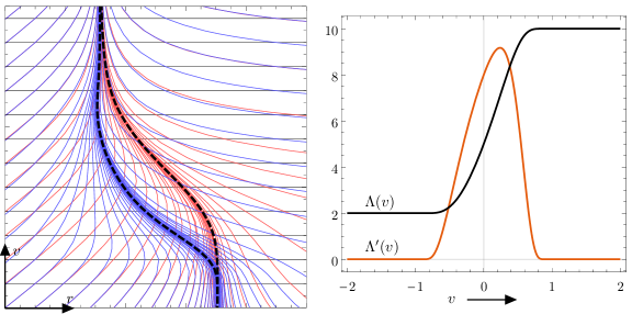
Figure 3: Null radial geodesics (left panel) for a null shell generated by a smooth curvature field $\Lambda(v)$ given in the right panel. The common ingoing null radial geodesics are horizontal lines in black. The outgoing geodesics of $g$ are depicted in red while the outgoing geodesics of $f$ are in blue.

Treating the $f$-sector in a similar manner, we find that the stress-energy tensor $T_{\mu\nu}^{f}=-V_{\mu\nu}^{f}$ comprises the following physical components,

$$\mu_{f}=-\alpha^{-2}\lambda^{-4}(v)\,\mu_{g},\qquad\rho_{f}=\lambda^{-2}(v)\,\rho_{g},\qquad p_{f}=\lambda^{-2}(v)\,p_{g},$$ (68)

with the equation of state $w_{f}=p_{f}/\rho_{f}=w_{g}=-1$. The null energy condition for the $f$-sector is similarly $T_{\mu\nu}^{f}k_{f}^{\mu}k_{f}^{\nu}=\frac{1}{2}\mathrm{e}^{2(x-y)}\mu_{f}\geq 0$ with $\rho_{f}+p_{f}=0$. Importantly, the signs of $\mu_{g}$ and $\mu_{f}$ are opposite, so the null energy conditions for the two sectors are strongly anticorrelated, in agreement with Baccetti:2012re . The two null energy conditions can only be simultaneously fulfilled for $\mu_{g}=\mu_{f}=0$, which happens whenever $\Lambda(v)=\mathrm{const}$.

Note that the violation of the null energy condition is intrinsic for the effective stress-energy tensors in the bimetric theory and does not automatically render the solutions nonphysical Baccetti:2012re . Also, the usage of energy conditions in GR is motivated largely by technical requirements about minimal assumptions needed to prove certain theorems (e.g., the singularity theorems, the positive energy theorem, or superluminal censorship), and many interesting GR solutions violate some of the energy conditions Visser:1999de ; Martin-Moruno:2017exc . In the ghost-free bimetric theory, similar considerations are more involved and the implications of the energy conditions need further investigation.

3 Discussion

In this paper we employed vacuum to denote an empty space in the absence of nongravitational fields. This is on the line with the majority of bimetric literature Schmidt-May:2015vnx ; deRham:2014zqa . In GR, however, the term vacuum has a slightly different connotation. A vacuum solution is a spacetime where the Ricci (or Einstein) tensor vanishes identically, $R_{\mu\nu}=0$ Stephani:2009exact ; Griffiths:2009exact ; Petrov:1969einstein , which means that the stress-energy tensor also vanishes identically. Also, an Einstein solution is a spacetime where the Ricci tensor is proportional to the metric, $R_{\mu\nu}\propto g_{\mu\nu}$. In such a case, the Einstein field equations are supplemented by a cosmological constant term (for this reason, Einstein spaces are sometimes denoted as lambdavacuum solutions). Hence, one has to be careful when talking about vacuum solutions in the bimetric context while referring to GR results. In GR, Birkhoff’s theorem is strictly stated for vacuum, $R_{\mu\nu}=0$, and can be extended to the cosmological constant case. In bimetric theory, the cosmological constant case holds whenever the bimetric potential $V(S)$ is constant. As shown, a similar extension of the theorem does not work when $V(S)$ varies.

As noted, the condition on the $\beta$-parameters (30) is the same as in the context of partially massless (PM) bimetric gravity, so an intriguing question arises about a possible relation between the found solutions and PM. In our case, the origin of (30) is the requirement that $\lambda(v)$ is an arbitrary function which satisfies the equation (27). In the PM case, the similar equation is posed for de Sitter background with a proportionality constant $c$ between the metrics $f=c^{2}g$ Hassan:2012gz . The requirement for $c$ to be undetermined by the background equation imposes the PM parameter choice. Treating the question of whether the candidate nonlinear theory can have the full PM gauge symmetry beyond the de Sitter background, the authors of Hassan:2012gz pointed out that the theory specified by (30) has an additional nonlinear gauge symmetry for a particular nonproportional homogeneous and isotropic vacuum solution. That solution is nonstationary and spherically symmetric admitting six Killing vectors fields. As in our case, the solution can be parametrized by an arbitrary function, enabled by (30). (Since the explicit form of that solution is not given in Hassan:2012gz , some of its geometrical properties are derived in appendix B for comparison.) Such a similarity to Hassan:2012gz makes our solution a suitable choice for a non-Einstein background in the context of the candidate PM theory.

If the PM parameters (30) are not imposed, the equation (27) requires $\lambda(v)=\mathrm{const}$. Then, $\lambda$ is determined as a solution of the quartic equation (27) depending on arbitrary $\beta$-parameters. Furthermore, the integration constant $b_{0}$ (introduced in Step 5 on page 2.2) can be chosen arbitrarily. This gives two Schwarzschild-(anti)de Sitter metrics having different Killing horizons and cosmological constants in general. Such solutions are encountered in Babichev:2015xha and considered in Torsello:2017zz in the context of symmetries in bimetric theory.

Another comment is about the choice of the principal square root branch $\lambda(v)>0$ in the ansatz (13). Noting that the potential $V(S)$ in (2) is a homogeneous function of $S$, a sign change of $\lambda$ is equivalent to the reparametrization $\beta_{n}\to(-1)^{n}\beta_{n}$. Note also that the signs of the $\mathrm{d}v\mathrm{d}r$-components in (13) need not be correlated for the two metrics as a general assumption. However, if the signs are different, the square root (17) will be purely imaginary, in which case substituting $\lambda\to\mathrm{i}\lambda$ and $G\to-G$ yields the same equations of motion as earlier. This poses no problem if the $\beta$-parameters satisfy (30) since $\beta_{1}$ and $\beta_{3}$ are identically zero. Nevertheless, the signature of the metric $f$ is changed to $(+,-,-,-)$ while the signature of $g$ remains $(-,+,+,+)$, which takes such a solution out of the scope of this paper.

Relinquishing spherical symmetry, the solution can be made axially symmetric using the Newman-Janis algorithm Newman:1965tw based on a trick with a complex coordinate transformation. The application of the algorithm on $g$ is summarized at the end of appendix A. The resulting axially symmetric metric reads,

$$g =-G(v,r,\theta)\,\mathrm{d}v^{2}+2\,\mathrm{d}v\mathrm{d}r+2a\sin^{2}\theta\,\mathrm{d}r\mathrm{d}\phi-2a\sin^{2}\theta\left(1-G(v,r,\theta)\right)\,\mathrm{d}v\mathrm{d}\phi$$

$$\qquad+\,\rho^{2}\mathrm{d}\theta^{2}+\left[\rho^{2}+a^{2}\sin^{2}\theta\left(2-G(v,r,\theta)\right)\right]\sin^{2}\theta\,\mathrm{d}\phi^{2},$$ (69)

where $\rho^{2}\coloneqq r^{2}+a^{2}\cos^{2}\theta$, $G(v,r,\theta)\coloneqq 1-\frac{1}{3}\Lambda(v)r^{4}/\rho^{2}$, and $a$ is a real constant that parametrizes the deviation from spherical symmetry along $\theta$ (for $a=0$, the metric is spherically symmetric). Constructing the square root,

$$S =\lambda(v)\left[\,\partial_{v}\otimes\mathrm{d}v+\partial_{r}\otimes\mathrm{d}r+\partial_{\theta}\otimes\mathrm{d}\theta+\partial_{\phi}\otimes\mathrm{d}\phi\,\right]$$

$$\qquad+\,r\lambda^{\prime}(v)\left[\,\partial_{r}\otimes\mathrm{d}v+a\sin^{2}\theta\,\partial_{r}\otimes\mathrm{d}\phi\,\right].$$ (70)

we obtain $f$ in a similar form as $g$ in (69),

$$f =\lambda^{2}(v)\Bigl{\{}-F(v,r,\theta)\,\mathrm{d}v^{2}+2\,\mathrm{d}v\mathrm{d}r+2a\sin^{2}\theta\,\mathrm{d}r\mathrm{d}\phi-2a\sin^{2}\theta\left(1-F(v,r,\theta)\right)\,\mathrm{d}v\mathrm{d}\phi$$

$$\qquad+\,\rho^{2}\mathrm{d}\theta^{2}+\left[\rho^{2}+a^{2}\sin^{2}\theta\left(2-F(v,r,\theta)\right)\right]\sin^{2}\theta\,\mathrm{d}\phi^{2}\Bigl{\}},$$ (71)

where $F(v,r,\theta)=G(v,r,\theta)+2r\lambda^{\prime}(v)/\lambda(v)$. The square root (70) differs from (32) in the presence of a new off-diagonal component $?{\mbox{$S$}}^{r}{}_{\phi}?=ar\sin^{2}\theta\lambda^{\prime}(v)$, which will contribute to the effective stress-energy $V_{g}$ with the off-diagonal component,

$$?{\mbox{$V_{g}$}}^{r}{}_{\phi}?=-\frac{1}{3}\Lambda^{\prime}(v)r\,a\sin^{2}\theta.$$ (72)

The Einstein tensors of $g$ and $f$ will have complicated forms (the explicit form of $G_{g}$ can be found in Ibohal:2004kk ), with the resulting $G_{g}+V_{g}$ and $G_{f}+V_{f}$ being nonzero. These can be matched with additional stress-energy tensors having off-diagonal components with nonvanishing rotation as a part of the modified energy flux, energy density and pressure.

Finally, we comment on the relation to GR solutions. The bimetric potential $V(S)$ of the found solution is a nondynamical field that is not governed by equations of motion. Thus the two sectors are dynamically decoupled, similarly to a bi-Einstein space setup with a constant $V(S)$ Hassan:2014vja ; Kocic:2017wwf . Here, however, we have two GR sectors each sourced by its own stress-energy tensor, where the two stress-energy tensors are related by (6). For our solution, the stress-energy tensors are of the generalized Vaidya type, as noted in subsection 2.5. In GR, the Vaidya metric is a solution of the Einstein field equations describing the spacetime of a spherically symmetric inhomogeneous imploding (exploding) null dust fluid Vaidya:1951zza . It is a nonstatic generalization of the Schwarzschild solution and admits only three independent Killing vector fields. The Vaidya metric is given by (13a) with $G(v,r)=1-2m(v)/r$ and $p=0$, where $m(v)$ is called the mass function, related to the gravitational energy within a given radius $r$ Lake:1991bff ; Poisson:1990eh . Note also that, unlike the Vaidya metric, our solution does not have a $1/r$ term. The mass function $m(v)$ can be generalized to depend also on the radial coordinate $r$ as in Husain:1995bf and Wang:1998qx . In the latter work, the mass function was considered to be expanded in the powers of $r$ as,

$$m(v,r)=\sum_{n=-\infty}^{\infty}a_{n}(v)\,r^{n},$$ (73)

where $a_{n}(v)$ are arbitrary functions depending only on $v$. Such generalized Vaidya solutions were further analyzed in Ibohal:2004kk ; Ibohal:2006ez ; Ibohal:2009px in the context of nonstationary de Sitter cosmological models (both spherically and axially symmetric). One particular model considered a mass function with $a_{3}(v)=\frac{1}{6}\Lambda(v)$ and $a_{n\neq 3}(v)=0$, which coincides with our solution (34a). In bimetric theory, however, such a model naturally comes out with a more specific form of $\Lambda(v)$ (33) whenever two spherically symmetric metrics share a common null direction in empty space.

Appendices

Appendix A Chart transition maps

In this appendix, we provide three chart transition maps; the first diagonalizes the metric $g$, the second puts the metric $g$ into a conformally flat form, and the third is a complex coordinate transformation trick which generates an axially symmetric from a spherically symmetric metric.

Chart 1.

Consider a chart transition map from $(v,r,\theta,\phi)$ to $(T,R,\theta,\phi)$ that diagonalizes $g$, so that,

$$g=-a(T,R)\,\mathrm{d}T^{2}+b(T,R)\,\mathrm{d}R^{2}+r^{2}\mathrm{d}\Omega^{2}.$$ (74)

Assuming that the coordinate transformation is achieved through functions $T(v,r)$ and $R(v,r)$, we have,

$$\mathrm{d}T =\partial_{v}T(v,r)\,\mathrm{d}v+\partial_{r}T(v,r)\,\mathrm{d}r,$$ (75a)

$$\mathrm{d}R =\partial_{v}R(v,r)\,\mathrm{d}v+\partial_{r}R(v,r)\,\mathrm{d}r.$$ (75b)

Substituting (75) in (74), then equating with (31a), gives the system of partial differential equations,

$$0 =1-\frac{1}{3}\Lambda(v)\,r^{2}+b(v,r)\left(\partial_{v}R(v,r)\right)^{2}-a(v,r)\left(\partial_{v}T(v,r)\right)^{2},$$ (76a)

$$0 =1-2b(v,r)\,\partial_{r}R(v,r)\,\partial_{v}R(v,r)+2a(v,r)\,\partial_{r}T(v,r)\,\partial_{v}T(v,r),$$ (76b)

$$0 =b(v,r)\left(\partial_{r}R(v,r)\right)^{2}-a(v,r)\left(\partial_{r}T(v,r)\right)^{2}.$$ (76c)

From the last two equations we can solve for $a(v,r)$ and $b(v,r)$ in terms of $\partial_{r}T(v,r)$, $\partial_{r}R(v,r)$ and the Jacobian $J=\partial_{v}T(v,r)\partial_{r}R(v,r)-\partial_{r}T(v,r)\partial_{v}R(v,r)$,

$$a(v,r)=-\frac{\partial_{r}R(v,r)}{J\,\partial_{r}T(v,r)},\qquad b(v,r)=-\frac{\partial_{r}T(v,r)}{J\,\partial_{r}R(v,r)}.$$ (77)

Substituting $a(v,r)$ and $b(v,r)$ in (76a) yields,

$$\frac{1}{3}\Lambda(v)\,r^{2}=1+\frac{\partial_{v}R(v,r)}{\partial_{r}R(v,r)}+\frac{\partial_{v}T(v,r)}{\partial_{r}T(v,r)}.$$ (78)

Note that the variables cannot be separated because of the mixed term $\Lambda(v)r^{2}$. Nonetheless, the above equation can have many solutions; one is easily obtained by splitting the right hand side in two parts,

$$1+\frac{\partial_{v}R(v,r)}{\partial_{r}R(v,r)}=0,\qquad\frac{\partial_{v}T(v,r)}{\partial_{r}T(v,r)}=\frac{1}{3}\Lambda(v)\,r^{2}.$$ (79)

This gives (with integration constants suppressed),

$$R(v,r)=r-v,\qquad T(v,r)=-\frac{1}{r}+\beta_{2}\intop\left(\alpha^{-2}+\lambda^{2}(v)\right)\mathrm{d}v,$$ (80)

which yields,

$$a(v,r)=\frac{-r^{2}}{r^{-2}+\beta_{2}\left(\alpha^{-2}+\lambda^{2}(v)\right)},\qquad b(v,r)=\frac{-r^{-2}}{r^{-2}+\beta_{2}\left(\alpha^{-2}+\lambda^{2}(v)\right)}.$$ (81)

As a final step, we express $a(r,v)$ and $b(r,v)$ in terms of $T$ and $R$ by inverting (80), which is a nontrivial task highly dependent on the form of $\lambda(v)$. Note that the chart transition (80) is valid for the nonvanishing Jacobian determinant $r^{-2}+\beta_{2}\left(\alpha^{-2}+\lambda^{2}(v)\right)$ (note that $r=0$ is not part of the spherical chart).

To avoid inverting (80), a more direct chart transition can be devised by fixing $a$, $b$ and $R$ in (74) as,

$$a(T,R)\coloneqq\varphi^{2}(T,R)\,G(T,R),\quad b(T,R)\coloneqq G(T,R)^{-1},\quad R(v,r)\coloneqq r,$$ (82)

so that $G(T,R)=\left(1-\frac{1}{3}\Lambda(t,r)\,r^{2}\right)^{-1}$. Here, we used the freedom to express $\lambda(v)$ and $\Lambda(v)$ in terms of a new arbitrary field $\lambda(T,R)$. Plugging in (75) into (74), then equating with (31a), we obtain the conditions,

$$\frac{\partial_{v}T(v,r)}{\partial_{r}T(v,r)}+G(v,r)=0,\qquad\varphi(v,r)=\frac{1}{G(v,r)\,\partial_{r}T(v,r)}.$$ (83)

Replacing the coordinate scalar $T$ by $t$ in terms of $\lambda(t,r)$ so that,

$$\frac{1}{\partial_{r}T(v,r)}\mathrm{d}T\coloneqq\frac{\partial_{t}\lambda(t,r)}{\partial_{r}\lambda(t,r)}\mathrm{d}t,$$ (84)

and further setting $\mathrm{d}\lambda=\partial_{t}\lambda(t,r)\,\mathrm{d}t+\partial_{r}\lambda(t,r)\,\mathrm{d}r$, we have,

$$\mathrm{d}v\coloneqq\frac{\mathrm{d}\lambda}{G(t,r)\,\partial_{r}\lambda(t,r)}=\frac{1}{G(t,r)}\frac{\partial_{t}\lambda(t,r)}{\partial_{r}\lambda(t,r)}\mathrm{d}t+\frac{1}{G(t,r)}\mathrm{d}r.$$ (85)

Substituting the above $\mathrm{d}v$ in (34a) yields a familiar form of the metric in the spherical chart $(t,r,\theta,\phi)$,

$$g=-\varphi^{2}(t,r)\left(1-\frac{1}{3}\Lambda(t,r)\,r^{2}\right)\mathrm{d}t^{2}+\left(1-\frac{1}{3}\Lambda(t,r)\,r^{2}\right)^{-1}\mathrm{d}r^{2}+r^{2}\mathrm{d}\Omega^{2},$$ (86)

where $\mathrm{d}\Omega^{2}=\mathrm{d}\theta^{2}+\sin^{2}\theta\,\mathrm{d}\phi^{2}$, $\Lambda(t,r)=3\beta_{2}\left(\alpha^{-2}+\lambda^{2}(t,r)\right)$ and,

$$\varphi(t,r)=\frac{\partial_{t}\lambda(t,r)}{\partial_{r}\lambda(t,r)}\left(1-\frac{1}{3}\Lambda(t,r)\,r^{2}\right)^{-1}.$$ (87)

Chart 2.

In the following, we provide a procedure to find a chart transition map which puts the metric $g$ into a conformally flat form,

$$g=\psi^{2}(T,R)\,\left[-\mathrm{d}T^{2}+\mathrm{d}R^{2}+R^{2}\mathrm{d}\Omega^{2}\right].$$ (88)

The coordinate transformation is achieved through functions $T(v,r)$ and $R(v,r)$ using (75). Plugging in (75) into (88), then equating with (31a), we obtain the condition $\psi(v,r)=-r/R(v,r)$ and the following system of partial differential equations,

$$0 =1-\frac{1}{3}\Lambda(v)\,r^{2}+\frac{r^{2}}{R^{2}(v,r)}\left[\left(\partial_{v}R(v,r)\right)^{2}-\left(\partial_{v}T(v,r)\right)^{2}\right],$$ (89a)

$$0 =R^{2}(v,r)-r^{2}\left[\partial_{r}R(v,r)\,\partial_{v}R(v,r)-\partial_{r}T(v,r)\,\partial_{v}T(v,r)\right],$$ (89b)

$$0 =\left(\partial_{r}R(v,r)\right)^{2}-\left(\partial_{r}T(v,r)\right)^{2}.$$ (89c)

Introducing new coordinate scalars $U$ and $V$ through

$$T(v,r)=U(v,r)-V(v,r),\qquad R(v,r)=U(v,r)+V(v,r),$$ (90)

from (89c) we get $\partial_{r}U(v,r)\,\partial_{r}V(v,r)=0$. As a consequence, either $U$, $V$ or both do not depend on $r$. Setting $V(v,r)=V(v)$ yields,

$$0 =\left(1-\frac{1}{3}\Lambda(v)\,r^{2}\right)\left(U(v,r)+V(v)\right)^{2}+4r^{2}U(v,r)\,V^{\prime}(v),$$ (91a)

$$0 =\left(U(v,r)+V(v)\right)^{2}-2r^{2}V^{\prime}(v)\,\partial_{r}U(v,r).$$ (91b)

From (91b) we can solve,

$$U(v,r)=\frac{2r\,V^{\prime}(v)}{1-r\,W^{\prime}(v)\,V^{\prime}(v)}-V(v),$$ (92)

where $W(v)$ is an arbitrary integration function. Substituting $U(v,r)$ in (91a), then expanding as a series in $r$, yields the system,

$$0 =W^{\prime}(v)V^{\prime}(v)+\frac{V^{\prime\prime}(v)}{V^{\prime}(v)},$$ (93a)

$$\frac{1}{3}\Lambda(v) =\left[2W^{\prime\prime}(v)-W^{\prime}(v)^{2}V^{\prime}(v)\right]V^{\prime}(v).$$ (93b)

From (93a) we obtain,

$$V^{\prime}(v)=\frac{1}{W(v)+c_{1}},\qquad V(v)=\int V^{\prime}(v)\,\mathrm{d}v+c_{2},$$ (94)

where $c_{1}$ and $c_{2}$ are integration constants. Substituting in (93b) gives,

$$2W^{\prime\prime}(v)\,\left[W(v)-c_{1}\right]-W^{\prime}(v)^{2}-\frac{1}{3}\Lambda(v)\left[W(v)-c_{1}\right]^{2}=0.$$ (95)

This equation can be solved for $W$ depending on the form of $\Lambda(v)$. Using $W$ from (95), $V$ from (94), and $U$ from (92) yields,

$$\varphi(v,r)=\frac{1}{2}\left(r\,W^{\prime}(v)-\frac{1}{V^{\prime}(v)}\right)\!,\qquad R(v,r)=\frac{2r\,V^{\prime}(v)}{1-r\,W^{\prime}(v)\,V^{\prime}(v)},$$ (96)

where $T(v,r)=R(v,r)-2V(v)$. As a final step, one should express $\varphi(v,r)$ in terms of $T$ and $R$ by inverting (80), which nontrivally depends on the form of $\Lambda(v)$.

Generating an axially symmetric metric.

Here we follow the algorithm from Newman:1965tw to “derive” an axially symmetric metric from a known spherically symmetric one (see also Newman:1965my and section 2 in Ibohal:2004kk ). Consider a spherically symmetric metric of the form (34a),

$$g =-G\,\mathrm{d}v^{2}+2\,\mathrm{d}v\mathrm{d}r+r^{2}\left(\mathrm{d}\theta^{2}+\sin^{2}\theta\,\mathrm{d}\phi^{2}\right),$$ (97)

where $G=1-\frac{1}{3}\Lambda(v)r^{2}$. Allowing $r$ to take complex values (so that $\bar{r}$ is the complex conjugate of $r$), we formally perform the complex coordinate transformation,

$$V=v+\mathrm{i}a\cos\theta,\qquad R=r+\mathrm{i}a\cos\theta,$$ (98)

where $V$ and $R$ are considered to be real. Here, $a$ is a real constant that parametrizes the deviation from the spherical symmetry. Using the map (98) and a suitable substitution $\mathrm{d}\theta\leftrightarrow-\mathrm{i}\sin\theta\mathrm{d}\phi$ (prescribed in Ibohal:2004kk ), we get,

$$g =-G\,\mathrm{d}V^{2}+2\,\mathrm{d}V\mathrm{d}R+2a\sin^{2}\theta\,\mathrm{d}R\mathrm{d}\phi+2a\sin^{2}\theta\left(1-G\right)\,\mathrm{d}V\mathrm{d}\phi$$

$$\qquad+\,\left(R^{2}+a^{2}\cos^{2}\theta\right)^{2}\mathrm{d}\theta^{2}+\left[R^{2}+a^{2}+a^{2}\sin^{2}\theta\left(1-G\right)\right]\sin^{2}\theta\,\mathrm{d}\phi^{2},$$ (99)

where $G=1-\frac{1}{3}\Lambda(v)R^{4}/\left(R^{2}+a^{2}\cos^{2}\theta\right)$.

Note that the chart $(V,R,\theta,\phi)$ has a coordinate singularity at $R^{2}+a^{2}\cos^{2}\theta=0$. Finally, after conveniently replacing $V\to v$ and $R\to r$, we obtain (69).

Appendix B Nonproportional vacuum solution

To obtain a solution parametrized by an arbitrary function, the authors of Hassan:2012gz consider nonproportional homogeneous and isotropic backgrounds vonStrauss:2011mq ,

$$g=-\mathrm{d}t^{2}+a^{2}(t)\,h,\qquad f=-X^{2}(t)\mathrm{d}t^{2}+Y^{2}(t)\,h,$$ (100)

where $h$ is the spatial metric with the curvature $k$,

$$h=\frac{\mathrm{d}r^{2}}{1-kr^{2}}+r^{2}\left(\mathrm{d}\theta^{2}+\sin^{2}\theta\,\mathrm{d}\phi^{2}\right).$$ (101)

Here, $a(t)$, $Y(t)$ and $X(t)$ are three fields that parametrize the ansatz. In general, these functions can be solved for from the bimetric field equations vonStrauss:2011mq . In vacuum, the equation that determines $Y/a$ is identically zero provided the PM parameter choice (30) is satisfied. Consequently, one of the three functions in (100) is arbitrary. Note that this ansatz does not allow for an explicit stress-energy tensor in either $g$ or $f$, but does allow for it if both $g$ and $f$ have seperate $T_{\mu\nu}$ (similarly to the axially symmetric case). In this case however, the ratio $Y/a$ will be determined by an equation of motion.

For comparison to our solution, consider the equivalent ansatz,

$$g =-\mathrm{d}t^{2}+\mathrm{e}^{2a(t)}\,h,\qquad f=\lambda^{2}(t)\left[-X^{2}(t)\mathrm{d}t^{2}+\mathrm{e}^{2a(t)}\,h\right]\!.$$ (102)

Here, the field $\lambda(t)$ corresponds to $Y/a$ in (100). Also, the field $a(t)$ is replaced by $\mathrm{e}^{a(t)}$ to simplify equations. The bimetric field equations are,

$$0 =\left\langle\lambda\right\rangle_{0}^{3}-3a^{\prime 2},$$ (103a)

$$0 =\left\langle\lambda\right\rangle_{0}^{2}+X\left\langle\lambda\right\rangle_{1}^{2}-2a^{\prime\prime}-3a^{\prime 2},$$ (103b)

$$0 =\alpha^{-2}X^{2}\left\langle\lambda\right\rangle_{1}^{3}-3\lambda\left(\lambda a^{\prime}+\lambda^{\prime}\right)^{2},$$ (103c)

$$0 =\alpha^{-2}X^{2}\left(\langle\left\langle\lambda\right\rangle_{1}^{2}+X\langle\lambda\rangle_{2}^{2}\right)+2\lambda X^{\prime}\left(\lambda a^{\prime}+\lambda^{\prime}\right),$$ (103d)

$$\qquad-X\left[2\lambda\left(3a^{\prime}\lambda^{\prime}+\lambda^{\prime}\right)+\lambda^{2}\left(2a^{\prime\prime}+3a^{\prime 2}\right)+\lambda^{\prime 2}\right].$$ (103e)

where derivatives are with respect to $t$. The Bianchi constraint is,

$$\left\langle\lambda\right\rangle_{1}^{2}\left[\lambda^{\prime}+\left(\lambda-X\right)a^{\prime}\right]=0.$$ (104)

From the Bianchi constraint we have $X(t)=\lambda(t)+\lambda^{\prime}(t)/a^{\prime}(t)$. Then for the PM parameter choice (30), we obtain the solution,

$$a^{\prime}(t)^{2}=\beta_{2}\left(\alpha^{-2}+\lambda^{2}(t)\right),$$ (105)

where $\lambda(t)$ is an arbitrary function. Similarly to (33), we can define,

$$\Lambda(t)\coloneqq 3\beta_{2}\left(\alpha^{-2}+\lambda^{2}(t)\right).$$ (106)

Then $\Lambda(t)=3a^{\prime 2}(t)$ and $a(t)=\int\!\left(\Lambda(t)/3\right)^{1/2}\mathrm{d}t$. The resulting square root is in matrix notation,

$$S=\operatorname{diag}\left[\,\lambda(t)+\lambda^{\prime}(t)/a^{\prime}(t),\,\lambda(t),\lambda(t),\lambda(t)\,\right].$$ (107)

This gives the effective stress energy tensor $T_{\mu\nu}^{g}=-V_{\mu\nu}^{g}$ with the nonzero components,

$$\rho_{g}=T_{00}^{g}=\Lambda(t),\qquad p_{g}=T_{11}^{g}=-\left(\Lambda(t)+\frac{\Lambda^{\prime}(t)}{\sqrt{3\Lambda(t)}}\right)\exp\left[2\int\!\left(\Lambda(t)/3\right)^{1/2}\mathrm{d}t\right].$$ (108)

From the equation of state,

$$w_{g}=\frac{p_{g}}{\rho_{g}}=-\left(1+\frac{\Lambda^{\prime}(t)}{\sqrt{3}}\Lambda^{-3/2}(t)\right)\exp\left[2\int\!\left(\Lambda(t)/3\right)^{1/2}\mathrm{d}t\right].$$ (109)

Note that $\Lambda(t)$ is arbitrary and can be obtained from observations. Adjusting $\Lambda(t)$ can also be used to model inflationary scenarios. The solution is homogeneous and isotropic with six Killing vector fields. The chart map $\mathrm{d}\tilde{t}=\lambda(t)X(t)\mathrm{d}t$ puts the metric $f$ in a similar form as $g$, relating the Killing vector fields of the two sectors.