Analytic Methods to Find Beating Transitions of Asymmetric Gaussian Beams in GNLS equations

Abstract

In a simple model of propagation of asymmetric Gaussian beams in nonlinear waveguides, described by a reduction to ordinary differential eqautions of generalized nonlinear Schrödinger equations (GNLSEs) with cubic-quintic (CQ) and saturable (SAT) nonlinearities and a graded-index profile, the beam widths exhibit two different types of beating behavior, with transitions between them. We present an analytic model to explain these phenomena, which originate in a $1:1$ resonance in a 2 degree-of-freedom Hamiltonian system. We show how small oscillations near a fixed point close to $1:1$ resonance in such a system can be approximated using an integrable Hamiltonian and, ultimately, by a single first order differential equation. In particular, the beating transitions can be located from coincidences of roots of a pair of quadratic equations, with coefficients determined (in a highly complex manner) by the internal parameters and initial conditions of the original system. The results of the analytic model agree with numerics of the original system over large parameter ranges, and allow new predictions that can be verified directly. In the CQ case we identify a band of beam energies for which there is only a single beating transition (as opposed to $0$ or $2$) as the eccentricity is increased. In the SAT case we explain the sudden (dis)appearance of beating transitions for certain values of the other parameters as the grade-index is changed.

1 Introduction

In the sequence of papers [23, 22, 21] a variational approach was taken to investigate the propagation of asymmetric (elliptic) Gaussian beams in nonlinear waveguides, with cubic-quintic and saturable nonlinearities and a parabolic graded-index (GRIN) profile, as described by suitable generalized nonlinear Schrödinger equations (GNLSEs). The beam widths in the two transverse directions to the direction of propagation were found to obey a set of ordinary differential equations which can be identified as the equations of motion of a point particle in certain rather complicated, but tractable, 2d potentials. Numerical analysis of these equations revealed “beating” phenomena: in addition to fast oscillations, the beam widths exhibit a (relatively) slow periodic variation. Furthermore, two types of beating were identified: In type I beating the amplitude of oscillation of the beam width in one direction remains greater than the amplitude of oscillation in the other direction, whereas in type II, there is an interchange between the widths in the two transverse directions. The type of beating depends on the parameters of the system and initial eccentricity of the beam. Remarkably, as the initial eccentricty or other parameters are changed, there can be a transition between types, and this transition is characterized by a singularity in the ratio of the periods of the beating and of the fast oscillatory motion.

The intention of the current paper is to provide a theoretical analysis of the beating phenomena and, in particular, to present an approximate analytic method to find the transitions between types. The relevant tool is the analysis of small oscillations in $2$ degree-of-freedom Hamiltonian systems near a fixed point which is close to $1:1$ resonance. The fact that resonance is the source of “beating” or “energy transfer” phenomena in mechanical systems is well known. A classic example can be found in the paper of Breitenburger and Mueller [8] on the elastic pendulum, which the authors describe as a “paradigm of a conservative, autoparametric system with an internal resonance”. The paper [8] has other features in common with our work (such as the use of action-angle variables and the fact that the analytic approximation used is a single elliptic function equation) but it is in the much simpler context of $1:2$ resonance. For other examples of autoparametric resonance see, for example, [49, 18]. The most widely used tool for analysis of systems near resonance is the mutliple time scale method, see for example [28, 32] for thorough presentations and many examples. For a typical modern application see [50, 51]. However, averaging techniques present an alternative [43], and in the context of Hamiltonian systems, working in action-angle coordinates has substantial advantages [13]. A typical study of a system near resonance will involve looking at the bifurcations of special solutions. In this context much attention has been paid to the definition and identification of nonlinear normal modes — see [36] for a review, and [41] for an example in the context of $1:1$ resonance.

The $2$ degree-of-freedom Hamiltonian systems we study have a discrete symmetry, and are approximated by a family of systems with $1:1$ resonance studied nearly $40$ years ago by Verhulst [48]. Verhulst showed the existence of an approximate second integral and used this to study bifurcations of special solutions and their stability. Our work differs from that of Verhulst and other works on $1:1$ resonance in several regards. The bifurcation question we pose depends not only on the internal parameters of the system, but also on the initial conditions. The question is not only one of identifying different types of solutions of the system, but also seeing how the type of solution changes as both the initial condition and internal system parameters are varied. We have not seen a similar study in the highly complex context of $1:1$ resonance. Our methodology uses action-angle variables and canonical transformations (though in an appendix we show how to apply standard two time scale techniques). Unlike in most existing studies, it is necessary to compute the relevant canonical transformation to second order. However, this does not affect the result that once the correct canonical transformation has been applied, the resulting approximating Hamiltonian depends only on a single combination of the angle variables and is integrable. The equations of motion for the integrable Hamiltonian can be reduced to a single first order differential equation, and the rich bifurcation structure of the systems we study can reduces to understanding the bifurcations of roots of a pair of quadratic polynomials, with coefficients that depend (in a complex, nonexplicit manner) on the internal parameters of the systems and the initial conditions. Comparison with numerical results shows our method gives high-quality results in a significant region of parameter space, and allows a variety of interesting new predictions.

The structure of this paper is as follows. In the next section we review the relevant models from nonlinear optics and the collective variable approximation to obtain equations for the propagation of beam widths, and present the main findings of papers [23, 22, 21] and some further numerical results. In section 3, we develop our method of integrable approximation for small oscillations in a $2$ degree-of-freedom Hamiltonian system near a fixed point close to $1:1$ resonance. In section 4 we describe the application of this method to the specific systems relevant to beam propagation, confirming existing numerical results and presenting new predictions. In section 5 we summarize and conclude. Appendix A completes some technical details omitted from the main text, and Appendix B describes an alternate method of approximation of the full equations using a two time expansion. This is a more ad hoc approach than the one explained in section 3, but we include it as it is more commonly used in the literature, and for certain values of parameters it gives better results.

Before closing this introduction we mention a number of points concerning the relevance of the work in this paper to optical solitons. We will describe in next section the manner in which we use ordinary differential equations (ODEs) to study the behavior of solutions of GNLSEs. The use of ODEs to study GNLSEs is widespread, see for example [44, 46, 3, 20, 45, 4] In particular, the last two papers use ODE methods in the study of rotating solitons. Our work extends the catalog of interesting bifurcations that can be observed in the context of GNLSEs; for another example; see the papers [17, 16] for a case of a saddle-loop bifurcation. Finally, we mention that we neglect dispersive terms in the GNLSEs we study. This is justifiable in the context of new optical materials [29, 39, 27, 11, 10] characterized by Kerr coefficients of the order $10^{-11}$–$10^{-12}$ ${\rm cm}^{2}/{\rm W}$, making the critical intensity for self-focusing small enough that it can be reached using microsecond pulses and possibly even continuous wave (CW) laser beams.

2 Models, the collective variable approach and numerical results

We consider beam propagation in a nonlinear, graded-index fiber, as described by one of the following GNLSEs:

$$2i\psi_{z}+\psi_{xx}+\psi_{yy}+\left(|\psi|^{2}-Q|\psi|^{4}-g(x^{2}+y^{2})\right)\psi = 0\ ,$$ (2.1)

$$2i\psi_{z}+\psi_{xx}+\psi_{yy}+\left(\frac{|\psi|^{2}}{1+\alpha^{2}|\psi|^{2}}-g(x^{2}+y^{2})\right)\psi = 0\ .$$ (2.2)

Here, modulo suitable normalizations [30, 21], $\psi$ is the strength of the electric field, $z$ is the longitdinal coordinate, $x,y$ are transverse coordinates, and $Q,\alpha,g$ are parameters. The first equation is the case of cubic-quintic nonlinearity (CQ), the second is the case of saturable nonlinearity (SAT). In the low intensity limit these models are similar, but for higher intensity they display different physical properties. In both cases, the higher order nonlinearity prevents beam collapse associated with the standard Kerr nonlinearity [9, 30]. The term $-g(x^{2}+y^{2})\psi$ reflects the graded-index nature of the fibre, that the refractive index $n$ falls with distance $r$ from the center of the fibre according to the law $n^{2}=n_{0}^{2}-Gr^{2}$; the physical significance of this is explained in [47, 14, 21].

The collective variable approximation (CVA), introduced for the study of self-focusing beams in [6, 7, 5], is a variational technique to approximate solutions of nonlinear Schrödinger-type equations which has been used and validated in many different situations [31]. The method replaces partial differential equations such as (2.1) and (2.2) by a system of ordinary differential equations for the coefficients of an ansatz for the full solution. The GNLSEs (2.1) and (2.2) are variational equations for action principles based on the Lagrangian densities

$${\cal L}_{\rm CQ} = i\left(\psi\psi^{*}_{z}-\psi^{*}\psi_{z}\right)+\left|\psi_{x}\right|^{2}+\left|\psi_{y}\right|^{2}-\frac{1}{2}|\psi|^{4}+\frac{Q}{3}|\psi|^{6}+g(x^{2}+y^{2})|\psi|^{2}\ ,$$ (2.3)

$${\cal L}_{\rm SAT} = i\left(\psi\psi^{*}_{z}-\psi^{*}\psi_{z}\right)+\left|\psi_{x}\right|^{2}+\left|\psi_{y}\right|^{2}+\frac{\ln\left(1+\alpha^{2}|\psi|^{2}\right)-\alpha^{2}|\psi|^{2}}{\alpha^{4}}+g(x^{2}+y^{2})|\psi|^{2}\ .$$

We assume $\psi$ takes the form of the trial function

$$\psi_{T}(x,y,z)=A(z)\exp\left(i\phi(z)-\frac{x^{2}}{2a_{x}^{2}(z)}+ib_{x}(z)x^{2}-\frac{y^{2}}{2a_{y}^{2}(z)}+ib_{y}(z)y^{2}\right)\ ,$$ (2.5)

where $A,\phi,a_{x},a_{y},b_{x},b_{y}$ are currently undetermined, real functions of only the longitudinal coordinate $z$. This trial function describes an elliptic Gaussian beam with $a_{x},a_{y}$ representing the widths of the beam in the $x,y$ directions. $b_{x},b_{y}$ describe curvatures of the beam wavefront, $A$ is the normalized amplitude of the electric field, and $\phi$ is a longitudinal phase factor. Our choice of a Gaussian shape for the trial function is appropriate because the Gaussian is an exact solution of the linear Schrödinger equation for GRIN waveguides [47, 14]. Substituting the trial function in the Lagrangian densities (2.3),(LABEL:lag2) and computing the integrals over the variables $x,y$ we obtain reduced densities for the functions $A,\phi,a_{x},a_{y},b_{x},b_{y}$. The corresponding Euler-Lagrange equations in the CQ case are

$$\dot{A} = -(b_{x}+b_{y})A\ ,$$

$$\dot{a}_{x,y} = 2a_{x,y}b_{x,y}\ ,$$

$$\dot{b}_{x,y} = \frac{1}{2a^{4}_{x,y}}-2b^{2}_{x,y}-\frac{g}{2}-\frac{A^{2}}{a^{2}_{x,y}}\left(\frac{1}{8}-\frac{QA^{2}}{9}\right)\ ,$$

$$\dot{\phi} = -\frac{1}{2a^{2}_{x}}-\frac{1}{2a^{2}_{y}}+\left(\frac{3}{8}-\frac{5QA^{2}}{18}\right)A^{2}\ .$$

Here a dot denotes differentiation with respect to $z$. In the SAT case the equations for $A,a_{x},a_{y}$ remain the same, but those for $b_{x},b_{y},\phi$ are replaced by

$$\dot{b}_{x,y} = \frac{1}{2a_{x,y}^{4}}-2b_{x,y}^{2}-\frac{g}{2}+\frac{\ln(1+\alpha^{2}A^{2})+\textrm{Li}_{2}(-\alpha^{2}A^{2})}{2\alpha^{4}A^{2}a_{x,y}^{2}}\ ,$$

$$\dot{\phi} = -\frac{1}{2a_{x}^{2}}-\frac{1}{2a_{y}^{2}}+\frac{\alpha^{2}A^{2}-2\ln(1+\alpha^{2}A^{2})-\textrm{Li}_{2}(-\alpha^{2}A^{2})}{2\alpha^{4}A^{2}}\ .$$

Here $\textrm{Li}_{2}(x)=\sum_{k=1}^{\infty}\frac{x^{k}}{k^{2}}$ is the Spence or dilogarithm function [1]. For both CQ and SAT cases we observe that $A^{2}a_{x}a_{y}$ is conserved [23, 22, 21], and we write $A^{2}a_{x}a_{y}=4E$ ($4E$ is the beam energy), and use this to eliminate $A(z)$ . Furthermore, $\phi(z)$ evidently plays no role in determining the other functions and can be computed by a simple quadrature once the other functions have been found. Furthermore, it is clear that we can write $b_{x}$ ($b_{y}$) in terms of $a_{x}$ ($a_{y}$) and its $z$-derivative. Thus we can reduce the system of $6$ equations to a pair of second order equations for $a_{x},a_{y}$. After some more calculation it emerges that the equations are simply the equations of motion

$$\ddot{a}_{x}=-\frac{\partial V}{\partial a_{x}}\ ,\qquad\ddot{a}_{y}=-\frac{\partial V}{\partial a_{y}}$$ (2.6)

for a particle in a potential $V(a_{x},a_{y})$, where for CQ

$$V=V_{CQ}\equiv\frac{1}{2}\left(\frac{1}{a_{x}^{2}}+\frac{1}{a_{y}^{2}}\right)-\frac{E}{a_{x}a_{y}}+\frac{16QE^{2}}{9a_{x}^{2}a_{y}^{2}}+\frac{g}{2}\left(a_{x}^{2}+a_{y}^{2}\right)\ ,$$ (2.7)

and for SAT

$$V=V_{SAT}\equiv\frac{1}{2}\left(\frac{1}{a_{x}^{2}}+\frac{1}{a_{y}^{2}}\right)-\frac{a_{x}a_{y}}{4E\alpha^{4}}{\rm Li}_{2}\left(-\frac{4E\alpha^{2}}{a_{x}a_{y}}\right)+\frac{g}{2}\left(a_{x}^{2}+a_{y}^{2}\right)\ .$$ (2.8)

Thus integration of equations (2.6) for potentials (2.7) and (2.8) provides a first approximation to solutions of the GNLSEs (2.1) and (2.2). Full numerical solutions of GNLSEs have been given in both the SAT [52] and the CQ [35] cases with $g=0$. In [35] it was shown that the breathing frequencies found numerically are similar to those obtained by the CVA technique. In [52] it was shown that the shape of the beam obtained numerically for a saturable medium remains similar to Gaussian, even for an asymmetric initial condition. However, use of direct numeric methods to give an overall picture of the behavior of a GNLSE, as a function of all the various parameters, remains a computationally overwhelming task, and having an qualitatively correct analytic or semianalytic model is therefore useful for developing physical insight [30, 2].

Appropriate initial conditions for (2.6) are

$$a_{x}(0)=a_{0}r\ ,\qquad a_{y}(0)=\frac{a_{0}}{r}\ ,\qquad\dot{a_{x}}(0)=\dot{a_{y}}(0)=0\ .$$ (2.9)

The latter two conditions are equivalent to taking $b_{x}(0)=b_{y}(0)=0$. Note that both the CQ and the SAT system have a scaling symmetry

$$\begin{array}[]{lllll}a_{x}\rightarrow\lambda a_{x}\ ,&a_{y}\rightarrow\lambda a_{y}\ ,&a_{0}\rightarrow\lambda a_{0}\ ,&r\rightarrow r\ ,&z\rightarrow\lambda^{2}z\ ,\\ Q\rightarrow\lambda^{2}Q\ ,&\alpha\rightarrow\lambda\alpha\ ,&g\rightarrow\lambda^{-4}g\ ,&E\rightarrow E.&\end{array}$$ (2.10)

Thus for CQ we do not need to study the dependence of solutions on the $5$ parameters $Q,g,E,a_{0},r$, but only on the $4$ scale invariant quantities $Qa_{0}^{-2},ga_{0}^{4},E,r$. On occasion we will work with the scale invariant quantity $K_{\rm CQ}=4QEa_{0}^{-2}$ instead of the quantity $Qa_{0}^{-2}$. (For SAT, replace all instances of $Q$ in the previous two sentences with $\alpha^{2}$, and $K_{\rm SAT}=4\alpha^{2}Ea_{0}^{-2}$.) Note that since there is symmetry in both the models between $a_{x}$ and $a_{y}$, there is a $r\rightarrow\frac{1}{r}$ inversion symmetry, and thus we need only study $r\leq 1$ or $r\geq 1$.

In the papers [23, 22, 21] the ODE systems above were studied numerically. For appropriate choices of the parameters “beating” phenomena were observed: in addition to (relatively) fast “breathing” oscillations, the beam widths exhibit a (relatively) slow periodic variation. Two types of beating were identified: In type I beating, the amplitude of oscillation of the beam width in one direction remains greater than the amplitude of oscillation in the other direction. In type II beating, there is an interchange between the widths in the two transverse directions. This is illustrated in Figure 1, which shows solutions of the CQ system for $E=2.039$, $K_{\rm CQ}=0.71$, $ga_{0}^{4}=0.01$, and two choices of $r$: $r=1.14$ gives type I beating, whereas $r=1.16$ gives type II beating.

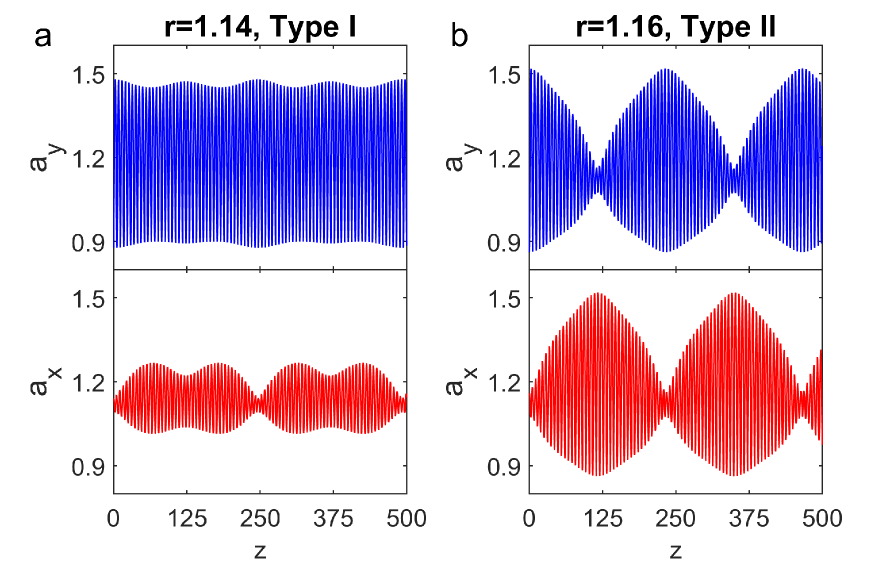
Figure 1: Two types of beating in the CQ system, with $E=2.039$, $K_{\rm CQ}=0.71$, $ga_{0}^{4}=0.01$. (a) For $r=1.14$ the amplitude of oscillation of $a_{y}$ is always more than that of $a_{x}$, this is type I beating. (b) For $r=1.16$ there is an exchange of roles, this is type II beating.

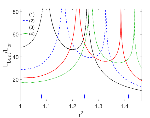
Figure 2: Dependence of the ratio of periods of slow beating and fast oscillatory motion, $L_{\rm beat}/L_{\rm br}$, on the parameter $r^{2}$ for the CQ model, and for various values of the parameter $ga_{0}^{4}$. $E=2.039$ and $K_{\rm CQ}=0.71$ throughout. (1) (dash-dot black) $ga_{0}^{4}=0$, (2) (dashed blue) $ga_{0}^{4}=0.01$, (3) (solid red) $ga_{0}^{4}=0.02$, (4) (dotted green) $ga_{0}^{4}=0.03$. Roman numerals indicate the type of beating in case (2), $ga_{0}^{4}=0.01$.

The type of beating depends on the parameters of the system and, as evident from Figure 1, on the initial eccentricity of the beam. Remarkably, as the initial eccentricty is increased, or as other parmeters are changed, there can be a transition between types. The approach to this transition is characterized by a divergence in the ratio of the periods of the slow beating and of the fast oscillatory motion. In Figure 2 this ratio (determined from numerical simulations) is plotted as a function of $r^{2}$ for the CQ system, with $E=2.039$, $K_{\rm CQ}=0.71$ and $ga_{0}^{4}=0,0.01,0.02,0.03$. (The reason for the choice of the coordinate $r^{2}$ on the $x$-axis is simply to make the plot clearer.) For $r$ just above $1$ the beating is type II, then there is a transition to type I, and then a second transition back to type II. The dependence on the system parameters of the two critical values of $r$, which we denote collectively by $r_{c}$, is explored further in Figure 3. In Figure 3a the values of $r_{c}$ are plotted as a function of $ga_{0}^{4}$ for three different values of $K_{\rm CQ}$ and a constant value of $E$; in Figure 3b $r_{c}$ is plotted as a function of $ga_{0}^{4}$ for three different values of $E$ and a constant value of $K_{\rm CQ}$. In general we see that $r_{c}$ increases as a function of $ga_{0}^{4}$ (for fixed $E,K_{\rm CQ}$). From Figure 3b we see that since the (solid) red is above the (dashed) blue is above the (dot-dashed) black, $r_{c}$ also increases as a function of $E$ (for fixed $ga_{0}^{4},K_{\rm CQ}$). But in Figure 3a we see there is difference between the upper and lower branches of $r_{c}$. We deduce that the higher value of $r_{c}$ also increases with $K_{\rm CQ}$ (for fixed $E,ga_{0}^{4}$), but the lower value decreases.

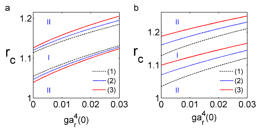
Figure 3: Dependence of $r_{c}$, the critical values of $r$, on system paramters $ga_{0}^{4},K_{\rm CQ},E$. (a) $r_{c}$ as a function of $ga_{0}^{4}$ for (1) $K_{\rm CQ}=0.602$ (dash-dot black), (2) $K_{\rm CQ}=0.71$ (dashed blue) and (3) $K_{\rm CQ}=0.739$ (solid red), all with $E=2.039$. (b) $r_{c}$ as a function of $ga_{0}^{4}$ for (1) $E=2.039$ (dash-dot black), (2) $E=2.079$ (dashed blue) and (3) $E=2.12$ (solid red), all with $K_{\rm CQ}=0.753$.

We shall see later that for other values of $ga_{0}^{4},K_{\rm CQ},E$ there can be just a single transition or no transitions at all as $r$ is increased from $1$. Transitions between beating types are also observed in the SAT system, again with a complex dependence on the parameters $ga_{0}^{4}$, $K_{\rm SAT}$ and $E$. The aim of this paper is to provide an integrable approximation for equations (2.6) with potentials (2.7) and (2.8) which provides a theoretical model to predict where the transitions between types take place.

3 Small oscillations near $1:1$ resonance

In this section we describe a general process of approximation near a $1:1$ resonance for a $2$ degree-of-freedom Hamiltonian system with Hamiltonian

$$H=\frac{1}{2}\left(p_{x}^{2}+p_{y}^{2}\right)+V(a_{x},a_{y})\ .$$ (3.1)

Here $a_{x},a_{y}$ are the coordinates, $p_{x},p_{y}$ are the conjugate momenta, and the potential $V$ (which typically will depend on a number of parameters) is symmetric, $V(a_{x},a_{y})=V(a_{y},a_{x})$. We assume that for typical values of the parameters the potential has an isolated symmetric minimum (at $a_{x}=a_{y}=a_{\rm min}$, say) at which the system is close to $1:1$ resonance. Note that because of the symmetry, $\displaystyle{\frac{\partial^{2}V}{\partial a_{x}^{2}}(a_{\rm min},a_{\rm min})=\frac{\partial^{2}V}{\partial a_{y}^{2}}(a_{\rm min},a_{\rm min})}$. Thus the Hessian matrix of the potential at $(a_{\rm min},a_{\rm min})$ has eigenvectors $\left(\begin{array}[]{c}1\\ \pm 1\end{array}\right)$ with eigenvalues $\displaystyle{\frac{\partial^{2}V}{\partial a_{x}^{2}}(a_{\rm min},a_{\rm min})\pm\frac{\partial^{2}V}{\partial a_{x}a_{y}}(a_{\rm min},a_{\rm min})}$. The condition for being close to $1:1$ resonance (i.e. equal eigenvalues) is therefore simply $\frac{\partial^{2}V}{\partial a_{x}a_{y}}(a_{\rm min},a_{\rm min})\approx 0$. For these systems we study orbits with initial conditions as given in (2.9).

The process of approximating such a system with an integrable system has $3$ steps.

The first step is to expand in normal coordinates near the fixed point, retaining only terms up to order $4$ in the potential. Thus we write

$$a_{x}=a_{\rm min}+\frac{\zeta_{2}+\zeta_{1}}{\sqrt{2}}\ ,\qquad a_{y}=a_{\rm min}+\frac{\zeta_{2}-\zeta_{1}}{\sqrt{2}}$$

and expand to fourth order to obtain

$$H_{1}=\frac{1}{2}\left(p_{1}^{2}+p_{2}^{2}+\omega_{1}^{2}\zeta_{1}^{2}+\omega_{2}^{2}\zeta_{2}^{2}\right)+a_{1}\zeta_{1}^{2}\zeta_{2}+a_{2}\zeta_{2}^{3}+a_{3}\zeta_{1}^{4}+a_{4}\zeta_{1}^{2}\zeta_{2}^{2}+a_{5}\zeta_{2}^{4}$$ (3.2)

where $p_{1},p_{2}$ are the conjugate momenta to the coordinates $\zeta_{1},\zeta_{2}$, and $\omega_{1},\omega_{2},a_{1},a_{2},a_{3},a_{4},a_{5}$ are constants that depend on the parameters of the original potential $V$. The Hamiltonian $H_{1}$ has $\zeta_{1}\rightarrow-\zeta_{1}$ symmetry as a consequence of the symmetry of $H$, and is the general Hamiltonian with this symmetry and a quartic potential. Aspects of the behavior of this Hamiltonian at, or close to, $1:1$ resonance have been studied previously, for example, in [48, 37, 38, 33, 40, 34]. The initial conditions for this system, corresponding to (2.9) are

$$\zeta_{1}(0)=\frac{a_{0}}{\sqrt{2}}\left(r-\frac{1}{r}\right)\ ,\qquad\zeta_{2}(0)=\frac{1}{\sqrt{2}}\left(a_{0}\left(r+\frac{1}{r}\right)-2a_{\rm min}\right)\ ,\qquad{p_{1}}(0)={p_{2}}(0)=0\ .$$ (3.3)

Symmetric solutions correspond to the initial condition $\zeta_{1}(0)=0$. In regarding $H_{1}$ as an approximation for $H$ we are neglecting terms of fifth order and above.

The second step is to make the canonical transformation to action-angle coordinates associated with the quadratic part of the Hamiltonian $H_{1}$, i.e. to substitute

$$\begin{array}[]{ll}\zeta_{1}=\sqrt{\frac{2J_{1}}{\omega_{1}}}\cos\theta_{1}\ ,&p_{1}=-\sqrt{2J_{1}\omega_{1}}\sin\theta_{1}\ ,\\ \zeta_{2}=\sqrt{\frac{2J_{2}}{\omega_{2}}}\cos\theta_{2}\ ,&p_{2}=-\sqrt{2J_{2}\omega_{2}}\sin\theta_{2}\ .\end{array}$$

This gives

$$H_{2} = \omega_{1}J_{1}+\omega_{2}J_{2}+\left(\frac{2J_{1}a_{1}}{\omega_{1}}+\frac{3J_{2}a_{2}}{\omega_{2}}\right)\sqrt{\frac{J_{2}}{2\omega_{2}}}\cos\theta_{2}$$ (3.4)

$$+\left(\frac{J_{2}}{2\omega_{2}}\right)^{3/2}2a_{2}\cos 3\theta_{2}+a_{1}\frac{J_{1}}{\omega_{1}}\sqrt{\frac{J_{2}}{2\omega_{2}}}\left(\cos(2\theta_{1}-\theta_{2})+\cos(2\theta_{1}+\theta_{2})\right)$$

$$+3a_{3}\frac{J_{1}^{2}}{2\omega_{1}^{2}}+a_{4}\frac{J_{1}J_{2}}{\omega_{1}\omega_{2}}+3a_{5}\frac{J_{2}^{2}}{2\omega_{2}^{2}}+a_{4}\frac{J_{1}J_{2}}{2\omega_{1}\omega_{2}}\left(\cos(2\theta_{1}-2\theta_{2})+\cos(2\theta_{1}+2\theta_{2})\right)$$

$$\left(2a_{3}\frac{J_{1}^{2}}{\omega_{1}^{2}}+a_{4}\frac{J_{1}J_{2}}{\omega_{1}\omega_{2}}\right)\cos(2\theta_{1})+a_{3}\frac{J_{1}^{2}}{2\omega_{1}^{2}}\cos(4\theta_{1})+\left(a_{4}\frac{J_{1}J_{2}}{\omega_{1}\omega_{2}}+2a_{5}\frac{J_{2}^{2}}{\omega_{2}^{2}}\right)\cos(2\theta_{2})$$

$$+a_{5}\frac{J_{2}^{2}}{2\omega_{2}^{2}}\cos(4\theta_{2})\ .$$

Here $\theta_{1},\theta_{2}$ are the angle variables, and $J_{1},J_{2}$ the conjugate actions. The initial conditions for the action variables are

$$J_{1}(0)=\frac{a_{0}^{2}\omega_{1}}{4}\left(r-\frac{1}{r}\right)^{2}\ ,\qquad J_{2}(0)=\frac{\omega_{2}}{4}\left(a_{0}\left(r+\frac{1}{r}\right)-2a_{\rm min}\right)^{2}\ .$$ (3.5)

The initial conditions for the angle variables depend on the sign of $\zeta_{1}(0)$ and $\zeta_{2}(0)$. If $\zeta_{1}(0)>0$ ($\zeta_{2}(0)>0$) then, from (3.3) we should take $\theta_{1}(0)=0$ ($\theta_{2}(0)=0$) and otherwise $\theta_{1}(0)=\pi$ ($\theta_{2}(0)=\pi$). Due to the $\zeta_{1}\rightarrow-\zeta_{1}$ symmetry of $H_{1}$ the Hamiltonian $H_{2}$ has period $\pi$ (and not $2\pi$) as a function of $\theta_{1}$ and thus the choice of the $\theta_{1}$ initial condition is irrelevant. The choice of the $\theta_{2}$ initial condition, however, is important. We are introducing a non-physical discontinuity in the approximation procedure when the sign of $\zeta_{2}(0)$ changes, i.e. when $r+\frac{1}{r}=\frac{2a_{\rm min}}{a_{0}}$. We will see the effects of this later, in our results for the SAT potential.

The third step involves a canonical change of coordinates $(\theta_{1},\theta_{2},J_{1},J_{2})\rightarrow(\phi_{1},\phi_{2},K_{1},K_{2})$ defined by a generating function of the second type $G_{2}(\theta_{1},\theta_{2},K_{1},K_{2})$ [15], chosen to eliminate the nonresonant terms from the Hamiltonian (i.e. all the trigonometric terms of order $||J||^{3/2}$ or $||J||^{2}$ except the one involving $\cos(2\theta_{1}-2\theta_{2})$.) The full change of coordinates is given by

$$\begin{array}[]{ll}\phi_{1}={\displaystyle{\frac{\partial G_{2}}{\partial K_{1}}}}\ ,&J_{1}={\displaystyle{\frac{\partial G_{2}}{\partial\theta_{1}}}}\ ,\\[12.0pt] \phi_{2}={\displaystyle{\frac{\partial G_{2}}{\partial K_{2}}}}\ ,&J_{2}={\displaystyle{\frac{\partial G_{2}}{\partial\theta_{2}}}}\ .\end{array}$$ (3.6)

The generating function $G_{2}$ should be taken in the form

$$G_{2} = K_{1}\theta_{1}+K_{2}\theta_{2}+A_{1}\sin\theta_{2}+A_{2}\sin 3\theta_{2}+A_{3}\sin(2\theta_{1}-\theta_{2})+A_{4}\sin(2\theta_{1}+\theta_{2})$$

$$+A_{5}\sin 2\theta_{1}+A_{6}\sin 4\theta_{1}+A_{7}\sin 2\theta_{2}+A_{8}\sin 4\theta_{2}+A_{9}\sin 6\theta_{2}+A_{10}\sin(2\theta_{1}+2\theta_{2})$$

$$+A_{11}\sin(2\theta_{1}+4\theta_{2})+A_{12}\sin(4\theta_{1}+2\theta_{2})+A_{13}\sin(2\theta_{1}-4\theta_{2})+A_{14}\sin(4\theta_{1}-2\theta_{2})$$

where the coefficients $A_{1},\ldots,A_{14}$ are functions of $K_{1},K_{2}$, which are chosen to eliminate the nonresonant trigonometric terms in the Hamiltonian to required order. $A_{1},A_{2},A_{3},A_{4}$ are of order $||K||^{3/2}$ and $A_{5},\ldots,A_{14}$ are of order $||K||^{2}$. The calculations are long, but straightforward with the help of a symbolic manipulator, and the final Hamiltonian is found to be simply

$$H_{3}=\omega_{1}K_{1}+\omega_{2}K_{2}+b_{1}K_{1}^{2}+b_{2}K_{1}K_{2}+b_{3}K_{2}^{2}+(b_{4}K_{1}^{2}+b_{5}K_{1}K_{2})\cos\left(2(\phi_{1}-\phi_{2})\right)$$ (3.7)

where

$$b_{1} = \frac{3a_{{3}}}{2\omega_{1}^{2}}-\frac{a_{{1}}^{2}\left(8\omega_{{1}}^{2}-3\omega_{{2}}^{2}\right)}{4\omega_{1}^{2}\omega_{2}^{2}\left(2\omega_{1}-\omega_{2}\right)\left(2\omega_{1}+\omega_{2}\right)}$$

$$b_{2} = \frac{a_{{4}}}{\omega_{{1}}\omega_{{2}}}-\frac{3a_{1}a_{2}}{\omega_{1}\omega_{2}^{3}}-\frac{2a_{{1}}^{2}}{\omega_{{1}}\omega_{{2}}\left(2\omega_{{1}}-\omega_{{2}}\right)\left(2\omega_{{1}}+\omega_{{2}}\right)}$$

$$b_{3} = \frac{3a_{{5}}}{2\omega_{{2}}^{2}}-\frac{15a_{{2}}^{2}}{4\omega_{{2}}^{4}}$$ (3.8)

$$b_{4} = \frac{\left(\omega_{{2}}-\omega_{{1}}\right)a_{{1}}^{2}}{2\omega_{{1}}^{2}\omega_{{2}}^{2}\left(2\omega_{{1}}-\omega_{{2}}\right)}$$

$$b_{5} = \frac{a_{{4}}}{2\omega_{{1}}\omega_{{2}}}-\frac{a_{1}a_{2}(4\omega_{1}^{2}-3\omega_{1}\omega_{2}-4\omega_{2}^{2})}{2\omega_{{1}}\omega_{{2}}^{3}\left(2\omega_{{1}}-\omega_{{2}}\right)\left(2\omega_{{1}}+\omega_{{2}}\right)}-\frac{a_{1}^{2}}{\omega_{1}^{2}\omega_{2}(2\omega_{1}-\omega_{2})}\ .$$

The Hamiltonian $H_{3}$ given in (3.7) is an integrable approximation of the original Hamiltonian $H$ given in (3.1). $H_{3}$ is a normal form for the “natural” Hamiltonian $H_{1}$ at or near $1:1$ resonance. Note that in the case of exact resonance $\omega_{1}=\omega_{2}$ the coefficient $b_{4}$ vanishes. Also close to resonance, the corresponding term in $H_{3}$ is of lower order than the other terms, and in [33, 40, 34] it is omitted. However, we choose to retain it to avoid any assumption on the relative orders of magnitude of $|\omega_{1}-\omega_{2}|$ and $||K||$. The integrability of $H_{3}$ is evident, as it only depends on the modified angle variables $\phi_{1},\phi_{2}$ through the combination $\phi_{1}-\phi_{2}$. As a consequence the quantity $K_{1}+K_{2}$ is conserved, in addition to the Hamiltonian itself. We denote the value of the Hamiltonian by ${\cal E}$ and the value of $K_{1}+K_{2}$ by $P$ (these should be computed from the system parameters and initial conditions). The full equations of motion are

$$\dot{\phi}_{1}=\frac{\partial H_{3}}{\partial K_{1}} = \omega_{1}+2b_{1}K_{1}+b_{2}K_{2}+(2b_{4}K_{1}+b_{5}K_{2})\cos(2(\phi_{1}-\phi_{2}))\ ,$$ (3.9)

$$\dot{\phi}_{2}=\frac{\partial H_{3}}{\partial K_{2}} = \omega_{2}+b_{2}K_{1}+2b_{3}K_{2}+b_{5}K_{1}\cos(2(\phi_{1}-\phi_{2}))\ ,$$ (3.10)

$$\dot{K}_{1}=-\frac{\partial H_{3}}{\partial\phi_{1}} = 2K_{1}(b_{4}K_{1}+b_{5}K_{2})\sin(2(\phi_{1}-\phi_{2}))\ ,$$ (3.11)

$$\dot{K}_{2}=-\frac{\partial H_{3}}{\partial\phi_{2}} = -2K_{1}(b_{4}K_{1}+b_{5}K_{2})\sin(2(\phi_{1}-\phi_{2}))\ .$$ (3.12)

Using the two conservation laws it is possible to eliminate $K_{2}$ and $\phi_{1}-\phi_{2}$ from the $K_{1}$ equation of motion to get a single equation for $K_{1}$:

$$\dot{K}_{1}^{2} = -4((b_{1}-b_{2}+b_{3}+b_{4}-b_{5})K_{1}^{2}+((b_{2}-2b_{3}+b_{5})P-\omega_{2}+\omega_{1})K_{1}+b_{3}P^{2}+\omega_{2}P-{\cal E})$$

$$((b_{1}-b_{2}+b_{3}-b_{4}+b_{5})K_{1}^{2}+((b_{2}-2b_{3}-b_{5})P-\omega_{2}+\omega_{1})K_{1}+b_{3}P^{2}+\omega_{2}P-{\cal E})\ .$$

Equation (LABEL:K1e) is a central result of this paper. To solve (LABEL:K1e) it is necessary to translate the initial conditions for $J_{1},J_{2},\theta_{1},\theta_{2}$ into initial conditions for $K_{1},K_{2}$. This step requires details of the canonical tranformation. Due to their length, the full equations determining the initial values of $K_{1},K_{2}$ are given in Appendix A (equations (A.1)-(A.2)). Note there are two cases depending on whether $\theta_{2}(0)$ is $0$ or $\pi$. Note also that there is no guarantee that these equations will have a solution with real, positive $K_{1},K_{2}$. In the case of the SAT system, for a certain range of parameter values we have experienced numerical problems with the solution of (A.1)-(A.2), specifically for initial values of $J_{2}$ close to zero, close to the jump from $\theta_{2}=0$ to $\theta_{2}=\pi$. However, typically there are values of $K_{1}(0),K_{2}(0)$ close to the given values of $J_{1}(0),J_{2}(0)$.

Once the initial values of $K_{1},K_{2}$ have been computed, the values of the constants ${\cal E}$ and $P$ can be found and equation (LABEL:K1e) can be solved. The right hand side of (LABEL:K1e) is the product of two quadratic factors in $K_{1}$, with up to $4$ real roots, and typical solutions will be oscillatory between two roots. When there is a double root then there is the possibility of the period of the oscillation becoming infinite, marking a bifurcation in the solution. There are two ways that a double root can occur, by the vanishing of the discriminant of one of the quadratic factors, or by one of the roots of the first factor coinciding with one of the roots of the second. The discriminants of the quadratic factors are

$$\Delta_{1} = \left((b_{2}+b_{5})^{2}-4b_{3}(b_{1}+b_{4})\right)P^{2}+2\left((b_{2}-2b_{3}+b_{5})\omega_{1}+(-2b_{1}+b_{2}-2b_{4}+b_{5})\omega_{2}\right)P$$ (3.14)

$$+4(b_{1}-b_{2}+b_{3}+b_{4}-b_{5}){\cal E}+(\omega_{1}-\omega_{2})^{2}\ ,$$

$$\Delta_{2} = \left((b_{2}-b_{5})^{2}-4b_{3}(b_{1}-b_{4})\right)P^{2}+2\left((b_{2}-2b_{3}-b_{5})\omega_{1}+(-2b_{1}+b_{2}+2b_{4}-b_{5})\omega_{2}\right)P$$ (3.15)

$$+4(b_{1}-b_{2}+b_{3}-b_{4}+b_{5}){\cal E}+(\omega_{1}-\omega_{2})^{2}\ .$$

A simple algebraic manipulation shows that the first factor and second factor have coincident roots if either $\Delta_{3}=0$ or $\Delta_{4}=0$, where

$$\Delta_{3} = b_{3}P^{2}+\omega_{2}P-{\cal E}\ ,$$ (3.16)

$$\Delta_{4} = \frac{b_{1}b_{5}^{2}-b_{2}b_{4}b_{5}+b_{3}b_{4}^{2}}{(b_{4}-b_{5})^{2}}P^{2}+\frac{b_{4}\omega_{2}-b_{5}\omega_{1}}{b_{4}-b_{5}}P-{\cal E}\ .$$ (3.17)

From (LABEL:K1e), we see that the first case occurs when the repeated root is at $K_{1}=0$.

It should be emphasized that the occurence of a double root on the RHS of (LABEL:K1e) is a necessary condition for a bifurcation of the solution (giving rise to a transition between types) but not a sufficient condition. For example, if the solution is describing an oscillation on the interval between two adjacent roots of the RHS, and the two other roots outside this interval merge, this will have no effect on the solution. We illustrate, in Figure 4, with two concrete examples of equation (LABEL:K1e) emerging from the CQ system described in Section 2. In both cases $Qa_{0}^{-2}=0.077$ and $ga_{0}^{4}=0$; in the first case $r=1.01$ and in the second case $r=1.045$. In both cases we plot the roots of the RHS as a function of the single remaining parameter $E$. (The choice to plot the roots for fixed values of $Qa_{0}^{-2}$, $ga_{0}^{4}$ and $r$ and to vary $E$ is just an illustration; we could just as easilly vary any of the other parameters or a combination thereof.) In the first case there are $4$ points $P_{1},P_{2},P_{3},P_{4}$ at which there are double roots; however, transitions only occur at the two points $P_{1},P_{4}$ (marked in Figure 4 with large dots). In the second case there are $5$ points $P_{1},P_{2},P_{3},P_{4},P_{5}$ at which there are double roots; however, transitions only occur at the two points $P_{2},P_{4}$. In both cases, the first transition is from type II to type I, and the second transition is from type I to type II, as indicated by Roman numerals on the plot.

The theoretical explanation of this is as follows. In the first case, $r=1.01$, there are $4$ values of $E$ for which there is a double root. The points labelled $P_{3}$ and $P_{4}$ on the diagram are associated with the vanishing of the discriminant $\Delta_{2}$; the point labelled $P_{1}$ is a double root at $0$, associated with the condition $\Delta_{3}=0$, and the point labelled $P_{2}$ is associated with the vanishing of the discriminant $\Delta_{1}$. The motion takes place between the root that is at $K_{1}\approx 0.00015$ and an adjacent root: for values of $E$ below $P_{2}$ the adjacent root is below, for values of $E$ above $P_{2}$ the adjacent root is above. Thus the double root at $P_{1}$ indicates a value of $E$ for which there is a bifurcation, and the period of oscillation diverges. The double root at $P_{2}$ is a special solution for which $K_{1}$ and $K_{2}$ are constant (looking at (3.11)-(3.12) it can be seen that there are $3$ kinds of solution of this type, each corresponding to vanishing of one of the three factors on the RHS of this equation; these are related to the nonlinear normal modes of the system [36, 40, 34]). The point $P_{2}$ does not, however, give rise to a transition in behavior of the CQ system; the beating period diverges there, but the type does not change. The double root at $P_{3}$ also does not mark a transition. This is precisely the case described above, in which the oscillation is on the interval between 2 roots, and the other two roots outside this interval merge. The point $P_{4}$, however, does mark a second transition, from type I beating back to type II.

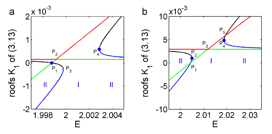
Figure 4: Roots of the RHS of (LABEL:K1e) as a function of $E$ for the case of (LABEL:K1e) emerging from the CQ system derived in Section 2, with $Qa_{0}^{-2}=0.077$, $ga_{0}^{4}=0$ and (a) $r=1.01$, (b) $r=1.045$. All double roots are labelled, but double roots leading to a transition are marked with large (blue) dots. In both plots, red and green curves indicate roots of the first quadratic factor in (LABEL:K1e), and blue and black curves indicate roots of the second quadratic factor.

Proceeding to the second example in Figure 4, there are now $5$ cases of a double root. $P_{2}$ and $P_{4}$ are associated with the vanishing of the discriminant $\Delta_{2}$, $P_{3}$ with the vanishing of the discriminant $\Delta_{1}$. $P_{1}$ is the case of a double root at zero associated with the condition $\Delta_{3}=0$, and $P_{5}$ is associated with the final possibility, $\Delta_{4}=0$. There are however only $2$ transitions, associated with the points $P_{2}$ and $P_{4}$, for similar reasons to the case described in the previous paragraph.

In this section we have explained how small oscillations of the original Hamiltonian (3.1) near its fixed point and near (symmetric) $1:1$ resonance can be approximated using the integrable Hamiltonian (3.7) and the single differential equation (LABEL:K1e). We have arrived at a simple analytic approximation for beating transitions, viz. a necessary condition for a transition between type I and type II beating is the vanishing of one of the four quantities $\Delta_{1},\Delta_{2},\Delta_{3},\Delta_{4}$ given in (3.14),(3.15),(3.16),(3.17). It should be emphasized that this far from trivializes the original problem. There is substantial complexity hidden in the relationship between parameters and initial conditions of the original Hamiltonian and those of the integrable Hamiltonian. Also determining which of the vanishing conditions gives a physical transition can be subtle. In Section 4 we apply the approximation to the CQ and SAT models from Section 2 and validate its predictions against numerical results.

4 Application to the models

4.1 The CQ Model

The potential of the CQ model, given by (2.7), has an isolated minimum when

$$a_{x}=a_{y}=a_{\rm min}\equiv\frac{4E\sqrt{2Q}}{3\sqrt{E-1}}C_{0}$$

where $C_{0}>0$ is a solution of the equation

$$1-C_{0}^{2}=\frac{1024E^{4}Q^{2}g}{81(E-1)^{3}}C_{0}^{6}\ .$$

The $1:1$ resonance condition is $E=E_{\rm res}$ where

$$E_{\rm res}=\frac{4}{1+\sqrt{1+\frac{65536Q^{2}g}{81}}}$$ (4.1)

In the case of zero grade index, $g=0$, we have $C_{0}=1$ and the resonance condition is simply $E=2$. The model is valid if the parameters $E,Q,g$ are chosen so that $E\approx E_{\rm res}$ and the initial conditions (see (2.9)) satisfy $a_{0}\approx a_{\rm min}$ and $r\approx 1$.

The relevant parameters for the quartic Hamiltonian (3.2) are

$$\omega_{1}^{2} = \frac{81}{512}\ \frac{(E-1)^{2}((2-E)C_{0}^{2}+E-1)}{E^{4}Q^{2}C_{0}^{6}}$$

$$\omega_{2}^{2} = \frac{81}{512}\ \frac{(E-1)^{3}(3-2C_{0}^{2})}{E^{4}Q^{2}C_{0}^{6}}$$

$$a_{1} = \frac{243}{8192}\ \frac{(E-1)^{5/2}\left(2(E-3)C_{0}^{2}-3(E-1)\right)}{{Q}^{5/2}C_{0}^{7}{E}^{5}}$$

$$a_{2} = \frac{243}{8192}\ \frac{(E-1)^{7/2}(2C_{0}^{2}-5)}{{Q}^{5/2}C_{0}^{7}{E}^{5}}$$ (4.2)

$$a_{3} = \frac{729}{262144}\ \frac{(E-1)^{3}(2(5-E)C_{0}^{2}+3(E-1))}{C_{0}^{8}{E}^{6}{Q}^{3}}$$

$$a_{4} = \frac{729}{131072}\ \frac{(E-1)^{3}\left(10(3-E)C_{0}^{2}+21(E-1)\right)}{C_{0}^{8}{E}^{6}{Q}^{3}}$$

$$a_{5} = \frac{3645}{262144}\ \frac{(E-1)^{4}(7-2C_{0}^{2})}{C_{0}^{8}{E}^{6}{Q}^{3}}$$

The detailed recipe for checking whether a given set of parameters and initial conditions $E,Q,g,a_{0},r$ might give rise to a transition is as follows:

1. Compute the coefficients $\omega_{1}^{2},\omega_{2}^{2},a_{1},a_{2},a_{3},a_{4},a_{5}$ using (4.2). This is the only stage of the recipe that is model dependent. Compute the coefficients $b_{1},b_{2},b_{3},b_{4},b_{5}$ from (3.8).

2. Compute the initial conditions $J_{1}(0),J_{2}(0)$ from (3.5) and $\theta_{1}(0),\theta_{2}(0)$ from the comments following (3.5). In the case of CQ, all the parameter values which we used gave $\theta_{1}(0)=0$ (we took $r>1$ throughout) and $\theta_{2}(0)=\pi$.

3. Compute the initial conditions $K_{1}(0),K_{2}(0)$ using (A.1)-(A.2). This is the only stage of the recipe that is not completely explicit, and involves solving two equations in two variables. If no real solution can be found, the method fails. A suitable initial guess for the solution is $K_{1}(0)\approx J_{1}(0)$ and $K_{2}(0)\approx J_{2}(0)$.

4. Determine the value of ${\cal E}$, the constant value of the Hamiltonian $H_{3}$ using (3.7), taking $\cos(2(\phi_{1}-\phi_{2}))=1$. Determine the value of $P=K_{1}+K_{2}$.

5. Compute $\Delta_{1},\Delta_{2},\Delta_{3},\Delta_{4}$ from (3.14),(3.15),(3.16),(3.17). Values of $E,Q,g,a_{0},r$ for which any of these quantities vanish are candidates for transitions.

Figure 5 displays results. Figure 5a shows numeric values and candidate analytic approximations of $r_{c}$ as a function of $E$ for $Qa_{0}^{-2}=0.077$ and $ga_{0}^{4}=0.01$. The dots denote numeric values of transitions in the original system. The solid curves show candidate analytic approximations of 3 distinct types: (1) (black) values for which $\Delta_{2}=0$ (a closed loop with a cusp on the axis at $r=1$), (2) (green) values for which $\Delta_{3}=0$ (a simple open curve) and (3) (red) values for which $\Delta_{4}=0$ (two crossing open curves). For the values of $Qa_{0}^{-2}$ and $ga_{0}^{4}$ specified, it seems there are two branches of parameter values for which there are transitions. We denote the lower branch (on the plot) by $r_{c,1}(E)$, which exists for $E$ greater than a certain value which we denote by $E_{c,1}$, and the upper branch by $r_{c,2}(E)$, which exists for $E$ greater than a certain value which we denote by $E_{c,2}$, with $E_{c,2}\approx 1.975<E_{c,1}\approx 1.977$. On the lower branch, as $E$ increases from $E_{c,1}$, $r_{c,1}(E)$ at first follows the approximation $\Delta_{2}=0$, until a triple point at which the curves $\Delta_{2}=0$ and $\Delta_{4}=0$ intersect. As $E$ increases further, $r_{c,1}(E)$ follows the approximation $\Delta_{4}=0$. Surprisingly, this approximation stays reasonably accurate for the full range shown on the figure, even though $r_{c,1}(E)$ rises to approximately $1.12$. On the upper branch, as $E$ increases from $E_{c,2}$, $r_{c,2}(E)$ at first follows the approximation $\Delta_{3}=0$, until a triple point at which the curves $\Delta_{2}=0$ and $\Delta_{3}=0$ intersect. As $E$ increases further, $r_{c,2}(E)$ follows the approximation $\Delta_{2}=0$. However, the quality of this approximation rapidly decreases as $E$ and $r_{c,2}(E)$ increase further, with the discrepancy already visible on the plot for $r_{c}\approx 1.06$.

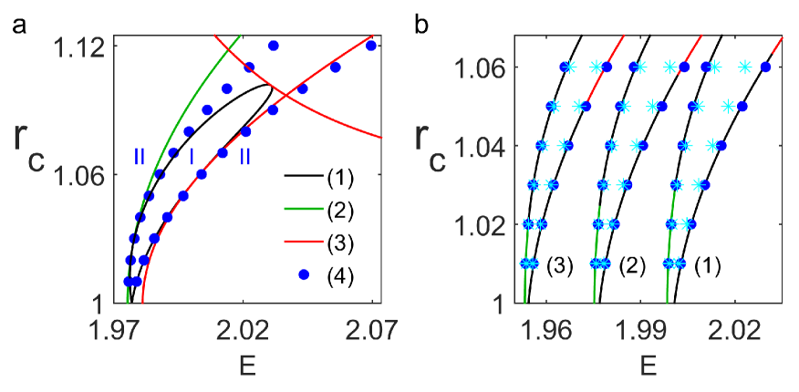
Figure 5: Comparison of numerics and analytic approximation for the CQ system. (a) (Blue) dots denote numerical results and curves denote candidate analytic approximations for $r_{c}$ as a function of $E$ for $Qa_{0}^{-2}=0.077$ and $ga_{0}^{4}=0.01$. Curve (1) (black) is $\Delta_{2}=0$, curve (2) (green) is $\Delta_{3}=0$, curve (3) (red) is $\Delta_{4}=0$. The correct analytic approximation is made up of pieces of all the curves, see text for full details. (b) (Blue) dots denote numerical results for the exact Hamiltonian (3.1), (turquoise) stars denote numerical results for the quartic Hamiltonian (3.2) and curves denote the analytic approximation for transitions, made up of pieces of the curves $\Delta_{2}=0$ (black), $\Delta_{3}=0$ (green), $\Delta_{4}=0$ (red). $Qa_{0}^{-2}=0.077$ throughout. (1) $ga_{0}^{4}=0$, (2) $ga_{0}^{4}=0.01$, (3) $ga_{0}^{4}=0.02$.

Figure 5b shows numeric values and the correct analytic approximation (made up of pieces of the curves $\Delta_{2}=0$, $\Delta_{3}=0$ and $\Delta_{4}=0$) in the cases (1) $ga_{0}^{4}=0$, (2) $ga_{0}^{4}=0.01$, (3) $ga_{0}^{4}=0.02$, all for $Qa_{0}^{-2}=0.077$. In addition, stars indicate numerical values of transitions obtained for the quartic system with Hamiltonian (3.2). For small values of $r$, the numerical values for transitions for the exact Hamiltonian and the approximate quartic Hamiltonian (3.2) are, as we would expect, very close. However as $r$ increases, we see that the results for the quartic Hamiltonian rapidly diverge from the results for the exact Hamiltonian, while, remarkably, the analytic approximation continues to be a reasonable approximation for the exact Hamiltonian. This may find an explanation in the fact that while the exact Hamitlonian (3.1), the quartic approximation (3.2) and the integrable approximation (3.7) all agree close to the fixed point, the global properties of the exact Hamiltonian are expected to be closer to those of the integrable approximation than the quartic approximation.

Note also in Figure 5b that the intercepts of the curves on the $E$ axis, that we have denoted above by $E_{c,1}$ and $E_{c,2}$, are very close to the values of $E$ determined by the resonance condition (4.1), which are (1) $E=2$, (2) $E\approx 1.977$, (3) $E\approx 1.954$. However, even though the intercepts for the two curves obtained for each set of parameter values are very close, they are not identical. This is something that is difficult to establish a priori by direct numerics for the original systems (as the beating periods, for values of $r$ close to $1$, are very long), but once the analytic approximation is available to give accurate candidate values for the transition locations, it is possible to verify them a posteriori. Thus in the small band of values $E_{c,2}<E<E_{c,1}$ there is only a single beating transition as the beam eccentricity is increased. As $r$ is increased from $1$ there is immediately type I beating, and as $r$ is increased further there is only a single transition to type II (as opposed, for example, to the sitution in Figure 2, where as $r$ is changed from $1$ type II beating is seen, and then there are two transitions). Using the analytic approximation it can be shown (see Appendix A) that the points $E_{c,1},E_{c,2}$ are determined by the conditions

$$\omega_{1}-\omega_{2}+P(b_{2}-2b_{3}\mp b_{5})=0$$ (4.3)

(minus for $E_{c,1}$, plus for $E_{c,2}$) for a solution with $r=1$. (The condition $r=1$ implies $J_{1}(0)=K_{1}(0)=0$, and then equation (A.2) gives a single equation from which to determine $K_{2}(0)$ from $J_{2}(0)=\omega_{2}\left(a_{0}-a_{\rm min}\right)^{2}$.) Figure 6 shows the dependence of $E_{c,1}$ and $E_{c,2}$ on $ga_{0}^{4}$ for two values of $Qa_{0}^{-2}$, as computed by the analytic approximation, along with a few numeric values (computed a posteriori). In addition the value of $E_{\rm res}$ from (4.1) is shown, this being the value of $E$ for which there is exact $1:1$ resonance in the linear approximation. We see that the values of $E_{c,1}$, $E_{c,2}$ and $E_{\rm res}$ all decrease monotonically with $ga_{0}^{4}$.

Figure 6: Dependence of $E_{c,1}$ and $E_{c,2}$ on $Qa_{0}^{-2}$ and $ga_{0}^{4}$, and comparison with the $E_{\rm res}$ from (4.1). (a) $Qa_{0}^{-2}=0.0836$ and (b) $Qa_{0}^{-2}=0.0924$. In both plots (1) (black, upper) shows numeric and analytic values of $E_{c,1}$, (2) (blue, middle) shows $E_{\rm res}$, and (3) (red, lower) shows numeric and analytic values of $E_{c,2}$.

4.2 The SAT Model

The potential of the SAT model, given by (2.8), has an isolated minimum when

$$a_{x}=a_{y}=a_{\rm min}\equiv a_{0}\sqrt{\frac{K_{\rm SAT}}{K_{0}}}$$

where $K_{0}$, which depends on the parameters $E,K_{\rm SAT},ga_{0}^{4}$, is a solution of the equation

$$\frac{K_{0}^{2}}{4E}+{\rm Li}_{2}(-K_{0})+\ln(1+K_{0})-\frac{K_{\rm SAT}^{2}ga_{0}^{4}}{4E}=0\ .$$ (4.4)

(Recall that the constant $K_{\rm SAT}$ is defined by $K_{\rm SAT}=4\alpha^{2}Ea_{0}^{-2}$.) The resonance condition can be written $K_{0}=K_{\rm res}$ where $K_{\rm res}$ is the solution of

$${\rm Li}_{2}(-K_{\rm res})+2\ln(1+K_{\rm res})-\frac{K_{\rm res}}{1+K_{\rm res}}=0\ .$$ (4.5)

$K_{\rm res}$ has numerical value approximately $5.017$. We recall that for our analytic model to be most effective we need to be near resonance, and the initial conditions should be close to the minimum, i.e. $a_{0}\approx a_{\rm min}$, or $K_{\rm SAT}\approx K_{0}$, and $r\approx 1$. These conditions give $K_{\rm SAT}\approx K_{\rm res}=5.017$ and $E\approx 6.550(1-ga_{0}^{4})$. In practice we will look at a large range of values of $E$ and $K_{\rm SAT}$, but focus on this region. We also recall that in our model the sign of $\zeta_{2}(0)$ (as given in (3.3) plays a critical role. From (4.4) we have $\zeta_{2}(0)=0$ (or equivalently $K_{\rm SAT}=K_{0}$) when [21]

$$E=\frac{-K_{\rm SAT}^{2}(1-ga_{0}^{4})}{4({\rm Li}_{2}(-K_{\rm SAT})+\ln(1+K_{\rm SAT}))}\ .$$ (4.6)

The relevant parameters for the quartic Hamiltonian (3.2) in the SAT case are

$$\omega_{1}^{2} = \frac{2}{a_{0}^{4}}\left(\frac{K_{0}^{2}}{K_{\rm SAT}^{2}}+ga_{0}^{4}\right)$$

$$\omega_{2}^{2} = \frac{4}{a_{0}^{4}K_{\rm SAT}^{2}}\left(-2E\ln(1+K_{0})+K_{0}^{2}+\frac{2EK_{0}}{1+K_{0}}\right)$$

$$a_{1} = \frac{\sqrt{2K_{0}}}{K_{\rm SAT}^{5/2}a_{0}^{5}}\left(2E\ln(1+K_{0})-3K_{0}^{2}-\frac{2EK_{0}}{1+K_{0}}\right)$$

$$a_{2} = \frac{\sqrt{2K_{0}}}{3K_{\rm SAT}^{5/2}a_{0}^{5}}\left(-2E\ln(1+K_{0})-3K_{0}^{2}+\frac{2EK_{0}(1+3K_{0})}{(1+K_{0})^{2}}\right)$$ (4.7)

$$a_{3} = \frac{K_{0}}{4K_{\rm SAT}^{3}a_{0}^{6}}\left(-2E\ln(1+K_{0})+5K_{0}^{2}+\frac{2EK_{0}}{1+K_{0}}\right)$$

$$a_{4} = \frac{K_{0}}{2K_{\rm SAT}^{3}a_{0}^{6}}\left(-2E\ln(1+K_{0})+15K_{0}^{2}+\frac{2EK_{0}(1-K_{0})}{(1+K_{0})^{2}}\right)$$

$$a_{5} = \frac{K_{0}}{12K_{\rm SAT}^{3}a_{0}^{6}}\left(2E\ln(1+K_{0})+15K_{0}^{2}-\frac{2EK_{0}(1+10K_{0}+K_{0}^{2})}{(1+K_{0})^{3}}\right)\ .$$

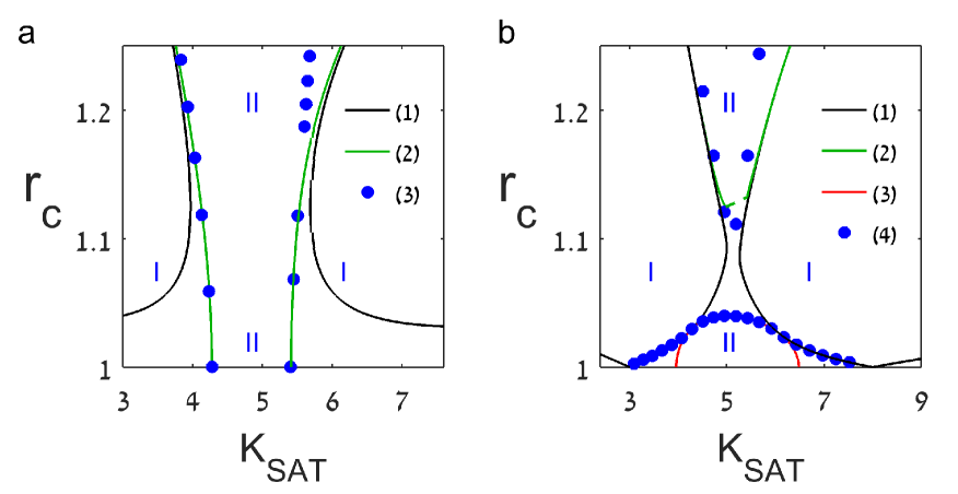
Figure 7: Behavior of $r_{c}$ as a function of $K_{\rm SAT}$ for the SAT model for fixed values of $E$ and $ga_{0}^{4}$, comparison of numerics and analytics. (a) (left) $E=6.3$, $ga_{0}^{4}=0$ (below the critical threshold). (b) (right) $E=6.7$, $ga_{0}^{4}=0$ (above the critical threshold). In both plots (blue) dots indicate transtions obtained from numerics of the original system. Curves denote different degeneracies in the analytic model: (1) (black) $\Delta_{2}=0$, (2) (green) $\Delta_{3}=0$, and (3) (red) $\Delta_{4}=0$ (for plot (b) only).

The method is identical to that given for CQ in the previous subsection, so we can immediately present results. For fixed values of $E$ and $ga_{0}^{4}$ we look for values of $r$ giving beating transitions as a function of $K_{\rm SAT}$. Both numeric and analytic results suggest there is a qualitative difference in behavior for $E$ above and below a critical threshold, and our results are consitent with the value of this threshold being approximately $6.550(1-ga_{0}^{4})$, as found above. Figure 7 displays results for $ga_{0}^{4}=0$ and $E=6.3$ (below the threshold, left) and $E=6.7$ (above the threshold, right). The numeric results show that below the threshold, there are two ranges of $K_{\rm SAT}$ for which there is a single beating transition, from type I (for $r$ below $r_{c}$) to type II (for $r$ above $r_{c}$). For values of $K_{\rm SAT}$ below or above these two ranges, there is only type I beating, and for values between the two ranges there is only type II beating. The analytic approximation reproduces these results well. In this region of parameter space there are values for which $\Delta_{2}=0$ (indicated in black in the figure) and $\Delta_{3}=0$ (indicated in green). It is the latter that are physically relevant, and the values of $r_{c}$ predicted by the analytic model are accurate for a good range. Moving “above the threshold”, numerics show there is a range of values of $K_{\rm SAT}$ for which, as $r$ is increased from $1$, the beating is initially type II, then there is a transition to type I. For some of these values there is then a further transition back to type II for quite high values of $r$. It should be mentioned that these latter transitions were initially discovered using the analytic approximation, and confirmed numerically a posteriori. The analytic approximation reproduces the first transition very well, using pieces of the $\Delta_{2}=0$ and $\Delta_{4}=0$ degeneracy curves. The upper transition is not reproduced well, which is not surprising bearing in mind the values of $r$ involved. Pieces of the $\Delta_{2}=0$ and $\Delta_{3}=0$ degeneracy curves are close to some of the results, but for a small range of values of $K_{\rm SAT}$ and $r$ the model fails as there is no solution of equations (A.1)-(A.2). Two branches of the $\Delta_{3}=0$ degeneracy curve come to an abrupt end (in the plot we have connected the ends with a dashed line, which is not associated with any degeneracy). The values of parameters involved are precisely those for which $\zeta_{2}(0)\approx 0$.

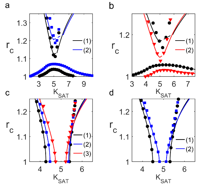
Figure 8: Behavior of $r_{c}$ as a function of parameters $K_{\rm SAT}$, $E$ and $ga_{0}^{4}$ for the SAT model, comparison of analytic approximation (curves) and numerics (blue dots). (a) $ga_{0}^{4}=0$, (1) (black) $E=6.7$, (2) (blue) $E=7.0$. (b) $ga_{0}^{4}=0.02$, (1) (black) $E=6.7$, (2) (red) $E=6.5$. (c) $ga_{0}^{4}=0$, (1) (black) $E=6.3$, (2) (blue) $E=6.4$, (3) (red) $E=6.5$. (d) $ga_{0}^{4}=0.02$, (1) (black) $E=6.3$, (2) (blue) $E=6.4$.

Figure 8 enlarges upon these results for different values of $E$ and $ga_{0}^{4}$. In the 4 panels here, the upper panels (a and b) show results for values of $E$ above the threshold, and the lower panels (c and d) show results for values of $E$ below the threshold. In the left panels (a and c), $ga_{0}^{4}=0$, in the right panels (b and d), $ga_{0}^{4}=0.02$. For $ga_{0}^{4}=0$, the values $E=6.3,6.4,6.5,6.7,7.0$ are shown, the first three of which are below the threshold (in panel c), and the last two above the threshhold (in panel a). For $ga_{0}^{4}=0.02$, the values $E=6.3,6.4,6.5,6.7$ are shown, the first two of which are below the threshold (in panel d), and the last two above the threshold (in panel b). Note specifically that for $ga_{0}^{4}=0$ the case $E=6.5$ is below the threshold (approximately $6.55$), while for $ga_{0}^{4}=0.02$ it is above (as the threshold drops to approximately $6.42$). Thus (for example) for $E=6.5$, $K_{\rm SAT}=5$ and $ga_{0}^{4}=0$, no beating transitions are observed as the beam eccentricity is increased; but if the grade index is changed to $ga_{0}^{4}=0.02$, there are two beating transitions. The analytic theory fully explains this phenomenon. Indeed, for all the cases shown in Figure 8, the analytic theory is in excellent quantitative agreement with numerics for lower values of $r$, and gives reasonable qualitative predictions for higher values of $r$.

Another conclusion from Figure 8 is that for values of $E$ below the threshold, we can find two values of $K_{\rm SAT}$ that give rise to a given value of $r_{c}$, but for $E$ above the threshold this need not be the case; furthermore the gap in $r_{c}$ values increases with the given value of $E$. In Figure 9 we illustrate this phenomenon more clearly. For the case $ga_{0}^{4}=0$, we show contours in the $K_{\rm SAT},E$ plane that give rises to the values $r_{c}=\frac{1}{0.95}\approx 1.053$ (black), $r_{c}=\frac{1}{0.92}\approx 1.087$ (blue) and $r_{c}=\frac{1}{0.895}\approx 1.117$ (red). It is clear that the “gap” between the two branches of each contour increases with $r$. Note that in the upper branch of each contour there is a small section denoted by a dashed line where the analytic method fails (the dashed line is a straight line between the last two points on each side for which the method works). As expected, the regions where the method fails straddle the curve (4.6), incidicated by a dashed turquoise curve. Note further that in many cases the analytic method works well far beyond the region in which this is expected, but there are some exceptions.

Figure 9: Contours of constant $r_{c}$ in the $K_{\rm SAT},E$ plane for the SAT model with $ga_{0}^{4}=0$, comparison of analytic approximation (curves) and numerics (data points). Red $r_{c}=\frac{1}{0.895}\approx 1.117$, blue $r=\frac{1}{0.92}\approx 1.087$, black $r=\frac{1}{0.95}\approx 1.053$. The upper dashed turquoise curve is the curve (4.6). In the case of a symmetric beam, this curve divides between periodic self-focusing (PSF) and periodic self-diffusing (PSD) solutions, see [22]. The lower dashed turquoise curve divides between PSD and monotonic diffracting (MD) solutions (in the case of symmetric beams; as asymmetry is introduced the curves moves).

5 Conclusions and discussion

In this paper we have described the beating phenomena observed in the equations of motion for the beam widths obtained in a collective variable approximation to solution of the GNLSEs relevant for beams in nonlinear waveguides with cubic-quintic (CQ) and saturable (SAT) nonlinearities and a graded-index profile. We have described the different types of beating, and the transitions between them. Arguing that the origin of these phenomena is in a $1:1$ Hamiltonian resonance, we have developed an approximation scheme for small oscillations in a class of 2 degree-of-freedom Hamiltonian systems with an isolated fixed point close to $1:1$ resonance. We have shown that such oscillations can be described by an integrable Hamiltonian, or, alternatively, a single first order differential equation (LABEL:K1e). Understanding the bifurcations of the system, which include the beating transitions, can be reduced to looking at the bifurcations of the roots of a pair of quadratic equations. Applying our general methodology to the specific cases of the CQ and SAT models we managed to reproduce numerical results for beating transitions over a large range of parameter values. The theory allows us to map out the regions (of parameter space and beam eccentricities) where beating transitions do and do not exist. Amongst other things, in the CQ case we identified a band of beam energies for which there is only a single beating transition (as opposed to $0$ or $2$) as the beam eccentricity is increased, and in the SAT case we explained the appearance and disappearance of transitions with changes of the grade-index.

We expect our methods to have applications to related problems in nonlinear optics, for nonlinearities other than the ones studied here, for different beams, such as super-Gaussian beams [24], and for optical bullets [30, 42]. We are encouraged by the fact that there is some recent experimental evidence [12] of breathing in optical solitons, albeit in a dissipative setting. We also hope the general theory of $1:1$ resonances that we have developed will find application in the settings of nonlinear mechanics and astronomy, as well as suitable extensions for $1:1:1$ resonances in higher dimensional systems (see for example the recent papers [25, 26]).

Appendix A Further Technical Details

As explained in section 3, the Hamiltonian (3.7) is in an integrable approximation to the Hamiltonian (3.4), and is obtained from (3.4) via a canonical transformation and neglecting higher order terms. The only need for explicit details of the canonical transformation is to compute the initial conditions of the variables $K_{1},K_{2}$ from the initial conditions of $J_{1},J_{2}$ given in (3.5). The equations to be solved are

$$J_{1} = K_{{1}}\mp{\frac{4K_{{1}}a_{{1}}}{4\omega_{{1}}^{2}-\omega_{{2}}^{2}}\sqrt{{\frac{2K_{{2}}}{\omega_{{2}}}}}}+\left(\frac{a_{1}^{2}\left(48\omega_{1}^{4}-8\omega_{1}^{3}\omega_{2}-40\omega_{2}^{2}\omega_{1}^{2}+2\omega_{1}\omega_{2}^{3}+5\omega_{2}^{4}\right)}{4\omega_{{2}}^{2}\omega_{{1}}^{3}\left(2\omega_{{1}}+\omega_{{2}}\right)^{2}\left(2\omega_{{1}}-\omega_{{2}}\right)^{2}}-{\frac{5a_{{3}}}{{2\omega_{{1}}}^{3}}}\right)K_{1}^{2}$$ (A.1)

$$+\left(\frac{\left(40\omega_{{1}}^{3}+28\omega_{{1}}^{2}\omega_{{2}}-6\omega_{{1}}\omega_{{2}}^{2}-3\omega_{{2}}^{3}\right)a_{{1}}^{2}}{\omega_{{1}}^{2}\omega_{{2}}\left(2\omega_{{1}}-\omega_{{2}}\right)^{2}\left(2\omega_{{1}}+\omega_{{2}}\right)^{2}\left(\omega_{{1}}+\omega_{{2}}\right)}\right.$$

$$\left.+\frac{\left(12\omega_{{1}}^{3}+11\omega_{{1}}^{2}\omega_{{2}}-10\omega_{{1}}\omega_{{2}}^{2}-6\omega_{{2}}^{3}\right)a_{{1}}a_{{2}}}{2\omega_{{1}}^{2}\omega_{{2}}^{3}\left(\omega_{{1}}+\omega_{{2}}\right)\left(4\omega_{{1}}^{2}-\omega_{{2}}^{2}\right)}-\frac{\left(3\omega_{{1}}+2\omega_{{2}}\right)a_{{4}}}{2\omega_{{1}}^{2}\omega_{{2}}\left(\omega_{{1}}+\omega_{{2}}\right)}\right)K_{1}K_{2}\ ,$$

$$J_{2} = K_{{2}}\mp 2\left(\frac{\left(2\omega_{{1}}^{2}-\omega_{{2}}^{2}\right)K_{{1}}a_{{1}}}{\omega_{{1}}\omega_{{2}}\left(4\omega_{{1}}^{2}-\omega_{{2}}^{2}\right)}+\frac{K_{{2}}a_{{2}}}{\omega_{{2}}^{2}}\right)\sqrt{\frac{2K_{{2}}}{\omega_{{2}}}}+\left(\frac{33a_{2}^{2}}{4\omega_{2}^{5}}-\frac{5a_{5}}{2\omega_{{2}}^{3}}\right)K_{2}^{2}$$ (A.2)

$$+\frac{\left(16\omega_{{1}}^{4}+8\omega_{{1}}^{3}\omega_{{2}}-12\omega_{{1}}^{2}\omega_{{2}}^{2}-2\omega_{{1}}\omega_{{2}}^{3}+3\omega_{{2}}^{4}\right){a_{{1}}}^{2}{K_{{1}}}^{2}}{2{\omega_{{1}}}^{2}\omega_{{2}}^{3}\left(2\omega_{{1}}-\omega_{{2}}\right)^{2}\left(2\omega_{{1}}+\omega_{{2}}\right)^{2}}$$

$$+\left(\frac{\left(8\omega_{{1}}^{4}+16\omega_{{1}}^{3}\omega_{{2}}-10\omega_{{1}}^{2}\omega_{{2}}^{2}-8\omega_{{1}}\omega_{{2}}^{3}+\omega_{{2}}^{4}\right){a_{{1}}}^{2}}{\omega_{{1}}^{2}\omega_{{2}}^{2}\left(2\omega_{{1}}-\omega_{{2}}\right)^{2}\left(2\omega_{{1}}+2\omega_{{2}}\right)^{2}\left(\omega_{{1}}+\omega_{{2}}\right)}\right.$$

$$\left.+\frac{\left(40\omega_{{1}}^{3}+44\omega_{{1}}^{2}\omega_{{2}}-9\omega_{{1}}\omega_{{2}}^{2}-16\omega_{{2}}^{3}\right)a_{{1}}a_{{2}}}{2\omega_{{1}}\omega_{{2}}^{4}\left(\omega_{{1}}+\omega_{{2}}\right)\left(2\omega_{{1}}-\omega_{{2}}\right)\left(2\omega_{{1}}+\omega_{{2}}\right)}-\frac{\left(2\omega_{{1}}+3\omega_{{2}}\right)a_{{4}}}{2\omega_{{1}}\omega_{{2}}^{2}\left(\omega_{{1}}+\omega_{{2}}\right)}\right)K_{1}K_{2}\ .$$

Here the upper signs should be taken in the square roots terms in the case $\theta_{2}(0)=0$ and the lower signs in the case $\theta_{2}(0)=\pi$.

In Section 4.1, in the study of the CQ system, we stated the conditions (4.3) for the value $r_{c}$ giving a beating transition to tend to $1$. We briefly describe the origin of these conditions. The symmetric solutions with $a_{x}=a_{y}$ of (2.6), arising from the initial condition $r=1$, correspond to solutions with $K_{1}\equiv 0$ of (3.9)-(3.12). From (LABEL:K1e), the values of $P$ and ${\cal E}$ for such a solution must evidently satisfy $b_{3}P^{2}+\omega_{2}P-{\cal E}=0$, which is just the condition $\Delta_{3}=0$, see (3.16). As explained in Section 3, a necessary condition for a beating transition is the vanishing of one of the quantites $\Delta_{1},\Delta_{2},\Delta_{3},\Delta_{4}$. To determine $E_{c,1}$ in Section 4.1 we want $r_{c}\rightarrow 1$ for a solution of $\Delta_{2}=0$. Clearly this requires $\Delta_{2}=\Delta_{3}=0$, and some simple algebra then gives the condition $\omega_{1}-\omega_{2}+P(b_{2}-2b_{3}-b_{5})=0$. To determine $E_{c,2}$, however, is not so straightforward, as for this we want we want $r_{c}\rightarrow 1$ for a solution of $\Delta_{3}=0$, and apparently we do not have two equations. The resolution of this conundrum is as follows: Although we stated above that the symmetric solutions of (2.6) correspond to solutions with $K_{1}\equiv 0$ of (3.9)-(3.12), the latter in fact provide a blow up of the former — there is a $3$ parameter family of the latter and only a $2$ parameter family of the former. Solving (3.9)-(3.12) in the case $K_{1}\equiv 0$, we obtain $K_{2}=P$ (constant), $\phi_{2}=\phi_{2}(0)+(\omega_{2}+2b_{3}P)z$, and that $\phi_{1}$ must satisfy the ODE

$$\dot{\phi}_{1}=\omega_{1}+b_{2}P+b_{5}P\cos\left(2\left(\phi_{2}(0)+(\omega_{2}+2b_{3}P)z-\phi_{1}\right)\right)\ .$$

This latter equation can be solved explicitly, and for a general choice of the constant of integration will give a complicated function $\phi_{1}(z)$. However, for a beating transition we seek a solution that is characterized by a single frequency, i.e. we need

$$\phi_{1}(z)=\phi_{1}(0)+(\omega_{2}+2b_{3}P)z$$

Substituting this in the differential equation, we obtain

$$\omega_{2}+2b_{3}P=\omega_{1}+b_{2}P+b_{5}P\cos\left(2\left(\phi_{2}(0)-\phi_{1}(0)\right)\right)\ .$$

Since the initial conditions $\phi_{1}(0),\phi_{2}(0)$ take the values $0$ or $\pi$, we deduce that $\omega_{1}-\omega_{2}+P(b_{2}-2b_{3}+b_{5})=0$, as required.

Appendix B A two time expansion approach

In this appendix we outline a two time expansion approach [28, 32] which is an alternative to the procedure based on canonical transformations given in Section 3.

We wish to look at solutions of the Hamiltonian system with Hamiltonian (3.1) and initial conditions (2.9). We assume the system has an isolated symmetric minimum at which the system is close to $1:1$-resonance. To apply a two time technique we need to introduce a small parameter $\epsilon$ explicitly into the equations. Our systems involve a number of system parameters, for example in the CQ case, the parameters $E,Q,g$, for which the resonance condition is (4.1). We introduce a small parameter by selecting one system parameter and writing this as its value at resonance plus a small perturbation. However, for reasons described in [48], the “small perturbation” here should be quadratic in the small parameter. Thus, for example in CQ, we have to consider two possibilities, $E=E_{\rm res}\pm\epsilon^{2}$ where $E_{\rm res}$ (which depends on the other system parameters $Q,g$) is the value of $E$ at resonance. The two resulting expansions will differ just in signs. This is the counterpart in the two time method of the need to choose $\theta_{2}(0)$ to be $0$ or $\pi$ in Section 3 and the resulting choice of signs in equations (A.1)-(A.2). However, we emphasize that it is not the same, so the resulting method is different, in particular, the “choice” in Section 3 involves the initial conditions as well as the system parameters.

Taking, as before, the minimum of the potential $V$ to be at $a_{x}=a_{y}=a_{\rm min}$ we now write

$$a_{x}=a_{\rm min}+\epsilon\tilde{a}_{x}\ ,\qquad a_{y}=a_{\rm min}+\epsilon\tilde{a}_{y}$$

and expand to 4th order in $\epsilon$. The order $0$ terms are irrelevant and can be discarded. The order $1$ terms vanish by definition of $a_{\rm min}$. In the other terms there is dependence on all the system parameters. However by making the assignment of the form $E=E_{\rm res}\pm\epsilon^{2}$, discarding all terms of order higher than $4$ and a suitable rescaling, we obtain an approximate potential of the form

$$\tilde{V} = \frac{1}{2}C_{1}(\tilde{a}_{x}^{2}+\tilde{a}_{y}^{2})+\epsilon\left(C_{2}(\tilde{a}_{x}^{3}+\tilde{a}_{y}^{3})+C_{3}\tilde{a}_{x}\tilde{a}_{y}(\tilde{a}_{x}+\tilde{a}_{y})\right)$$

$$+\epsilon^{2}\left(C_{4}(\tilde{a}_{x}^{4}+\tilde{a}_{y}^{4})+C_{5}\tilde{a}_{x}\tilde{a}_{y}(\tilde{a}_{x}^{2}+\tilde{a}_{y}^{2})+C_{6}\tilde{a}_{x}^{2}\tilde{a}_{y}^{2}+C_{7}(\tilde{a}_{x}^{2}+\tilde{a}_{y}^{2})+C_{8}\tilde{a}_{x}\tilde{a}_{y}\right)\ .$$

Here $C_{1},\ldots,C_{8}$ are all functions of the system parameters excluding the parameter replaced by $\epsilon$. Note that as a result of the dependence of the system parameters on $\epsilon$ there are now quadratic terms in $\tilde{a}_{x},\tilde{a}_{y}$ in the $O(\epsilon^{2})$ terms.

Following the usual two time formalism, we seek solutions of the system with potential $\tilde{V}$ in the form

$$\tilde{a}_{x} = \Lambda_{1}(\epsilon^{2}z)\cos(\sqrt{C_{1}}z)+\Lambda_{2}(\epsilon^{2}z)\sin(\sqrt{C_{1}}z)+\epsilon\tilde{a}_{x,1}(z,\epsilon^{2}z)+\epsilon^{2}\tilde{a}_{x,2}(z,\epsilon^{2}z)+\ldots$$

$$\tilde{a}_{y} = \Lambda_{3}(\epsilon^{2}z)\cos(\sqrt{C_{1}}z)+\Lambda_{4}(\epsilon^{2}z)\sin(\sqrt{C_{1}}z)+\epsilon\tilde{a}_{y,1}(z,\epsilon^{2}z)+\epsilon^{2}\tilde{a}_{y,2}(z,\epsilon^{2}z)+\ldots$$

Here $\Lambda_{1}(\epsilon^{2}z),\Lambda_{2}(\epsilon^{2}z),\Lambda_{3}(\epsilon^{2}z),\Lambda_{4}(\epsilon^{2}z)$ are functions of the slow variable $\epsilon^{2}z$. Substituting in the equations of motion and equating order-by-order, the first order terms $\tilde{a}_{x,1},\tilde{a}_{y,1}$ can be determined, and a system of first order equations is obtained that $\Lambda_{1},\Lambda_{2},\Lambda_{3},\Lambda_{4}$ must satisfy to guarantee the absence of secular terms in $\tilde{a}_{x,2},\tilde{a}_{y,2}$. Writing

$$R_{1} = \Lambda_{1}^{2}+\Lambda_{2}^{2}+\Lambda_{3}^{2}+\Lambda_{4}^{2}$$

$$R_{2} = \Lambda_{1}^{2}+\Lambda_{2}^{2}-\Lambda_{3}^{2}-\Lambda_{4}^{2}$$

$$R_{3} = \Lambda_{1}\Lambda_{3}+\Lambda_{2}\Lambda_{4}$$

$$R_{4} = \Lambda_{1}\Lambda_{4}-\Lambda_{2}\Lambda_{3}$$

(c.f. [41, 34, 19]) we obtain the system

$$R_{1}^{\prime} = 0$$

$$R_{2}^{\prime} = 4R_{4}(\gamma_{1}R_{1}+\gamma_{2}+(\gamma_{3}+\gamma_{4})R_{3})$$ (B.1)

$$R_{3}^{\prime} = -\gamma_{3}R_{2}R_{4}$$

$$R_{4}^{\prime} = -R_{2}(\gamma_{1}R_{1}+\gamma_{2}+\gamma_{4}R_{3})$$

where the constants $\gamma_{1},\gamma_{2},\gamma_{3},\gamma_{4}$ are certain combinations of the constants $C_{1},\ldots,C_{8}$. (Note $R_{3}^{2}+R_{4}^{2}=\frac{1}{4}(R_{1}^{2}-R_{2}^{2})$.) Thus $R_{1}$ is an invariant, as are the quantities

$$Q_{2}=R_{2}^{2}+4\left(1+\frac{\gamma_{4}}{\gamma_{3}}\right)\left(R_{3}+\frac{\gamma_{1}R_{1}+\gamma_{2}}{\gamma_{3}+\gamma_{4}}\right)^{2}\ ,\qquad Q_{3}=R_{4}^{2}-\frac{\gamma_{4}}{\gamma_{3}}\left(R_{3}+\frac{\gamma_{1}R_{1}+\gamma_{2}}{\gamma_{4}}\right)^{2}\ .$$

Note that $R_{1},Q_{2},Q_{3}$ are related by

$$Q_{2}+4Q_{3}=R_{1}^{2}-\frac{4(\gamma_{1}R_{1}+\gamma_{2})^{2}}{\gamma_{4}(\gamma_{3}+\gamma_{4})}\ .$$

Using the invariants it is possible to write a single differential equation for the quantity $R_{3}$:

$$(R_{3}^{\prime})^{2}=-4\gamma_{4}\left(\gamma_{3}+\gamma_{4}\right)\left(\left(R_{3}+\frac{\gamma_{1}R_{1}+\gamma_{2}}{\gamma_{3}+\gamma_{4}}\right)^{2}-\frac{\gamma_{3}}{4(\gamma_{3}+\gamma_{4})}Q_{2}\right)\left(\left(R_{3}+\frac{\gamma_{1}R_{1}+\gamma_{2}}{\gamma_{4}}\right)^{2}+\frac{\gamma_{3}Q_{3}}{\gamma_{4}}\right)\ .$$ (B.2)

This has the same form as (LABEL:K1e) — the right hand side is a product of two quadratic factors in $R_{3}$ — and similar techniques can be used to discuss bifurcations of its solutions. Specifically, there can be a double root if the discriminant of one of the factors vanishes (i.e. if $Q_{2}$ or $Q_{3}$ vanish), or if the factors have a common root. The latter happens in the two cases

$$\left((2\gamma_{1}\pm\gamma_{4})R_{1}+2\gamma_{2}\right)^{2}+4Q_{3}\gamma_{3}\gamma_{4}=0\ .$$ (B.3)

As in Section 3, detecting beating transitions requires translating the initial conditions to the constants of motion $R_{1},Q_{2},Q_{3}$ and checking up to $4$ conditions.

We have implemented this method for the CQ and SAT systems and found some satisfactory results which we do not report here; in certain cases the results were better than those found using the method based on canonical transformations. However there are numerous reasons to prefer the method based on canonical transformations. The two time method requires deciding how to explicitly introduce a small parameter and different ways of doing this give different results. It also requires advance knowledge of the correct relative order of magnitude of the oscillations around the fixed point and the deviation of the system parameters from their resonance values. In general, the algebraic manipulations required to implement the two time method, most of which we have omitted in our account here, are substantially more complicated than those required for the method based on canonical transformations; in particular the reduction of the system (B.1) to a single differential equation (B.2) is a surprise, that emerges from ad hoc manipulations, whereas the parallel steps in the canonical formalism are standard, based on the integrability of the Hamiltonian (3.7). Finally, from our numerical experiments it emerges that while the results based on the vanishing of the discriminant of one of the factors of the right hand side of (B.2) are good, the results based on conditions (B.3) are poor.

References

• [1] Abramowitz, M., and Stegun, I. A. Handbook of Mathematical Functions. Dover, New York, 1970.
• [2] Agrawal, G. P. Nonlinear Fiber Optics, 4th ed. Academic Press, New York, 2007.
• [3] Aleksic, B., Zarkov, B., Skarka, V., and Aleksi c, N. Stability analysis of fundamental dissipative Ginzburg-Landau solitons. Phys. Scr. T149 (2012), 014037.
• [4] Aleksi c, B. N., Aleksi c, N. B., Skarka, V., and Beli c, M. Stability and nesting of dissipative vortex solitons with high vorticity. Phys. Rev. A 91 (2015), 043832.
• [5] Anderson, D. Variational approach to nonlinear pulse propagation in optical fibers. Phys. Rev. A 27 (1983), 3135–3145.
• [6] Anderson, D., and Bonnedal, M. Variational approach to nonlinear self-focusing of gaussian laser beams. Phys. Fluids 22 (1979), 105–109.
• [7] Anderson, D., Bonnedal, M., and Lisak, M. Self-trapped cylindrical laser beams. Phys. Fluids 22 (1979), 1838–1840.
• [8] Breitenberger, E., and Mueller, R. D. The elastic pendulum: a nonlinear paradigm. J. Math. Phys. 22 (1981), 1196–1210.
• [9] Chen, Y. F., Beckwitt, K., Wise, F. W., and Malomed, B. A. Criteria for the experimental observation of multidimensional optical solitons in saturable media. Phys. Rev. E 70 (2004), 046610.
• [10] de Araújo, C. B., Gomes, A. S., and Boudebs, G. Techniques for nonlinear optical characterization of materials: a review. Reports on Progress in Physics 79 (2016), 036401.
• [11] de Oliveira, R. E. P., Sj din, N., Fokine, M., Margulis, W., de Matos, C. J. S., and Norin, L. Fabrication and optical characterization of silica optical fibers containing gold nanoparticles. ACS Applied Materials & Interfaces 7 (2015), 370–375.
• [12] Falcao-Filho, E. L., de Araújo, C. B., Boudebs, G., Leblond, H., and Skarka, V. Robust two-dimensional spatial solitons in liquid carbon disulfide. Phys. Rev. Lett. 110 (2013), 013901.
• [13] Gendelman, O., and Sapsis, T. Energy exchange and localization in essentially nonlinear oscillatory systems: canonical formalism. Journal of Applied Mechanics 84 (2017), 011009.
• [14] Ghatak, A. K., and Thyagarajan, K. Contemporary Optics. Plenum Press, New York, 1978.
• [15] Goldstein, H. Classical Mechanics. Adison-Wesley, Reading, MA, 1980.
• [16] Gomila, D., Jacobo, A., Matías, M. A., and Colet, P. Phase-space structure of two-dimensional excitable localized structures. Phys. Rev. E 75 (2007), 026217.
• [17] Gomila, D., Matías, M. A., and Colet, P. Excitability mediated by localized structures in a dissipative nonlinear optical cavity. Phys. Rev. Lett. 94 (2005), 063905.
• [18] Haller, G. Chaos near resonance, vol. 138 of Applied Mathematical Sciences. Springer-Verlag, New York, 1999.
• [19] Hanssmann, H., and Hoveijn, I. The 1:1 resonance in Hamiltonian systems. ArXiv e-prints (2017).
• [20] He, Y., and Malomed, B. A. Accessible solitons in complex Ginzburg-Landau media. Phys. Rev. E 88 (2013), 042912.
• [21] Ianetz, D., Kaganovskii, Y., and Wilson-Gordon, A. D. Dependence of beating dynamics on the ellipticity of a gaussian beam in graded-index absorbing nonlinear fibers. Phys. Rev. A 87 (2013), 043839.
• [22] Ianetz, D., Kaganovskii, Y., Wilson-Gordon, A. D., and Rosenbluh, M. Breathing dynamics of an asymmetric gaussian beam propagating in a saturable absorbing medium. Phys. Rev. A 82 (2010), 065803.
• [23] Ianetz, D., Kaganovskii, Y., Wilson-Gordon, A. D., and Rosenbluh, M. Propagation of an asymmetric gaussian beam in a nonlinear absorbing medium. Phys. Rev. A 81 (2010), 053851.
• [24] Jana, S., Singh, A., Porsezian, K., and Mithun, T. Self-trapped elliptical super-gaussian beam in cubic–quintic media. Opt. Commun. 332 (2014), 311–320.
• [25] Jayaprakash, K. R., and Starosvetsky, Y. Three-dimensional energy channeling in the unit-cell model coupled to a spherical rotator I: bidirectional energy channeling. Nonlinear Dynamics 89 (Aug 2017), 2013–2040.
• [26] Jayaprakash, K. R., and Starosvetsky, Y. Three-dimensional energy channeling in the unit-cell model coupled to a spherical rotator II: unidirectional energy channeling. Nonlinear Dynamics 89 (Sep 2017), 2311–2327.
• [27] Ju, S., Watekar, P. R., and Han, W. T. Fabrication of highly nonlinear germano-silicate glass optical fiber incorporated with pbte semiconductor quantum dots using atomization doping process and its optical nonlinearity. Opt. Express 19 (2011), 2599–2607.
• [28] Kevorkian, J., and Cole, J. D. Multiple scale and singular perturbation methods, vol. 114. Springer Science & Business Media, 2012.
• [29] Kim, Y. H., Lee, B. H., Chung, Y., Paek, U. C., and Han, W. T. Resonant optical nonlinearity measurement of ${\rm yb}^{3+}/{\rm al}^{3+}$ codoped optical fibers by use of a long-period fiber grating pair. Opt. Lett. 27 (2002), 580–582.
• [30] Kivshar, Y. S., and Agrawal, G. P. Optical Solitons. Academic Press, New York, 2003.
• [31] Malomed, B. A. Variational methods in nonlinear fiber optics and related fields. Prog. Opt. 43 (2002), 71–191.
• [32] Manevich, A. I., and Manevitch, L. I. The mechanics of nonlinear systems with internal resonances. Imperial College Press, London, 2005.
• [33] Marchesiello, A., and Pucacco, G. Relevance of the 1:1 resonance in galactic dynamics. Eur. Phys. Jour. Plus 126 (2011), 104.
• [34] Marchesiello, A., and Pucacco, G. Bifurcation sequences in the symmetric 1:1 Hamiltonian resonance. Internat. J. Bifur. Chaos Appl. Sci. Engrg. 26 (2016), 1630011.
• [35] Michinel, H., Campo-Taboas, J., Garca-Fern andez, R., Salgueiro, J. R., and Quiroga-Teixeiro, M. L. Liquid light condensates. Phys. Rev. E 65 (2002), 066604.
• [36] Mikhlin, Y. V., and Avramov, K. V. Nonlinears normal modes for vibrating mechanical systems. review of theoretical developments. Applied Mechanics Reviews 63 (2010), 060802.
• [37] Montaldi, J., Roberts, M., and Stewart, I. Existence of nonlinear normal modes of symmetric Hamiltonian systems. Nonlinearity 3 (1990), 695–730.
• [38] Montaldi, J., Roberts, M., and Stewart, I. Stability of nonlinear normal modes of symmetric Hamiltonian systems. Nonlinearity 3 (1990), 731–772.
• [39] Moon, S., Lin, A., Kim, B. H., R.Watekar, P., and Han, W. T. Linear and nonlinear optical properties of the optical fiber doped with silicon nano-particles. J. Non-Cryst. Solids 354 (2008), 602–606.
• [40] Pucacco, G., and Marchesiello, A. An energy-momentum map for the time-reversal symmetric $1:1$ resonance with $\mathbb{Z}_{2}\times\mathbb{Z}_{2}$ symmetry. Phys. D 271 (2014), 10–18.
• [41] Rand, R., Pak, C., and Vakakis, A. Bifurcation of nonlinear normal modes in a class of two degree of freedom systems. Acta Mech 3 (1992), 129–45.
• [42] Renninger, W., and Wise, F. Optical solitons in graded-index multimode fibres. Nature communications 4 (2013), 1719–1719.
• [43] Sanders, J. A., Verhulst, F., and Murdock, J. Averaging methods in nonlinear dynamical systems, second ed., vol. 59 of Applied Mathematical Sciences. Springer, New York, 2007.
• [44] Skarka, V., and Aleksic, N. B. Stability criterion for dissipative soliton solutions of the one-, two-, and three-dimensional complex cubic-quintic ginzburg-landau equations. Phys. Rev. Lett 96 (2006), 013903.
• [45] Skarka, V., Aleksi c, N. B., Leki c, M., Aleksi c, B. N., Malomed, B. A., Mihalache, D., and Leblond, H. Formation of complex two-dimensional dissipative solitons via spontaneous symmetry breaking. Phys. Rev. A 90 (2014), 023845.
• [46] Skarka, V., Timotijevic, D. V., and Aleksi c, N. B. Extension of the stability criterion for dissipative optical soliton solutions of a two-dimensional ginzburg-landau system generated from asymmetric inputs. J. Opt. A 10 (2008), 075102.
• [47] Sodha, M. S., and Ghatak, A. K. Inhomogeneous Optical Waveguides. Plenum Press, New York, 1977.
• [48] Verhulst, F. Discrete symmetric dynamical systems at the main resonances with applications to axi-symmetric galaxies. Phil. Trans. Roy. Soc. A 290 (1979), 435–465.
• [49] Verhulst, F. Parametric and autoparametric resonance. Acta Appl. Math. 70 (2002), 231–264.
• [50] Vorotnikov, K., and Starosvetsky, Y. Nonlinear energy channeling in the two-dimensional, locally resonant, unit-cell model. I. High energy pulsations and routes to energy localization. Chaos 25 (2015), 073106.
• [51] Vorotnikov, K., and Starosvetsky, Y. Nonlinear energy channeling in the two-dimensional, locally resonant, unit-cell model. II. Low energy excitations and unidirectional energy transport. Chaos 25 (2015), 073107.
• [52] Yang, J. Internal oscillations and instability characteristics of (2+1)-dimensional solitons in a saturable nonlinear medium. Phys. Rev. E 66 (2002), 026601.